A map-based method for eliminating systematic modes from galaxy clustering power spectra with application to BOSS

Abstract

We develop a practical methodology to remove modes from a galaxy survey power spectrum that are associated with systematic errors. We apply this to the BOSS CMASS sample, to see if it removes the excess power previously observed beyond the best-fit $\Lambda$CDM model on very large scales. We consider several possible sources of data contamination, and check whether they affect the number of targets that can be observed and the power spectrum measurements. We describe a general framework for how such knowledge can be transformed into template fields. Mode subtraction can then be used to remove these systematic contaminants at least as well as applying corrective weighting to the observed galaxies, but benefits from giving an unbiased power. Even after applying templates for all known systematics, we find a large-scale power excess, but this is reduced compared with that observed using the weights provided by the BOSS team. This excess is at much larger scales than the BAO scale and does not affect the main results of BOSS. However, it will be important for the measurement of a scale-dependent bias due to primordial non-Gaussianity. The excess is beyond that allowed by any simple model of non-Gaussianity matching Planck data, and is not matched in other surveys. We show that this power excess can further be reduced but is still present using "phenomenological" templates, designed to consider further potentially unknown sources of systematic contamination. As all discrepant angular modes can be removed using "phenomenological" templates, the potentially remaining contaminant acts radially.

1 Introduction

Galaxy surveys allow measurements that are crucial for our understanding of the Universe. For instance, Baryon Acoustic Oscillation (BAO) observations provide a standard ruler measurement that we can use to study our Universe’s expansion history, while Redshift Space Distortion (RSD) measurements test the theory of gravity that governs structure growth. Furthermore, a full measurement of the shape of the galaxy power spectrum provides additional information about the total matter density $\Omega_{\mathrm{m}}h^{2}$, the baryon density $\Omega_{\mathrm{b}}h^{2}$, the neutrino mass density $\Omega_{\mathrm{\nu}}h^{2}$, and the local primordial non-Gaussianity parameter $f_{\mathrm{NL}}$ (e.g. Slosar, Hirata, Seljak, Ho & Padmanabhan, 2008; Ross et al., 2013; Leistedt, Peiris & Roth, 2014).

While the field of density fluctuations revealed by galaxy surveys contains a lot of cosmological signal, this is contaminated by various foreground and instrumental sources. A simple model of such contaminations is that the true density field in Fourier space

$$D(\mathbf{k})=F(\mathbf{k})-\varepsilon f(\mathbf{k}),$$ (1)

is a linear combination of the measured density field $F(\mathbf{k})$ and the contaminant field that can be written in terms of a template $f(\mathbf{k})$ with unknown amplitude $\varepsilon$. In practice, we do not know the exact shape of $f(\mathbf{k})$ and the data is affected by more than one contaminant. This can be accounted for by extending Eq. (1) to include a range of different templates $f_{A}(\mathbf{k})$ with unknown amplitudes $\varepsilon_{A}$:

$$D(\mathbf{k})=F(\mathbf{k})-\sum_{A}\varepsilon_{A}f_{A}(\mathbf{k}).$$ (2)

Mode deprojection (Rybicki & Press, 1992) offers an elegant way of mitigating contaminants that can be modelled as in Eq. (2) by analytically marginalising over all $\varepsilon_{A}^{\mathrm{(true)}}$. This approach can directly be implemented in any covariance based estimator for the power spectrum, a natural choice being the Quadratic Maximum Likelihood (Tegmark, 1997, QML) Estimator whose estimates are unbiased and optimal for any covariance matrix. This technique has been applied by Slosar, Seljak & Makarov (2004) in angular power spectrum measurements from the Wilkinson Microwave Anisotropy Probe (WMAP) at low multipoles $\ell$, in investigating the Integrated Sachs-Wolfe (ISW) effect as a function of redshift (Ho, Hirata, Padmanabhan, Seljak & Bahcall, 2008), and by Pullen & Hirata (2013) to the SDSS quasar sample. Furthermore, Leistedt et al. (2013) identified, using mode deprojection, a previously found large-scale excess in the angular auto- and cross power spectra of the catalogue of photometric quasars from the Sixth Data Release (DR6) of SDSS as being due to systematics.

The computational cost of mode deprojection can be reduced by identifying the most important templates before marginalising over them as described by Leistedt & Peiris (2014). A complementary strategy to improve the computational efficiency of mode deprojection is to incorporate it into fast, but sub-optimal power spectrum estimators, such as the Feldman, Kaiser & Peacock (1994, FKP) Estimator for the 3D power spectrum, as described in Kalus et al. (2016). This work was subsequently extended to the Pseudo-$C_{\ell}$ (Hivon et al., 2002) Estimator for the angular power spectrum, by Elsner, Leistedt & Peiris (2017).

In this article, we consider how systematic templates can be produced for common systematic issues, using the Northern Galactic Cap (NGC) of the SDSS-III BOSS CMASS sample as our example data set. We derive a set of templates for this sample, and use the Mode Subtraction technique of Kalus et al. (2016) to remove these modes when making a power spectrum measurements of these data. The MOde Subtraction code to Eliminate Systematic contamination in galaxy clustering power spectrum measurements (MOSES) is available at https://github.com/KalusB/Moses.

The outline of this paper is as follows: In Sec. 2.2, we review the Mode Subtraction technique and develop a method to generate templates for a given contaminant and survey. We use this method to generate templates for known contaminants driven by: foreground stars (Sec. 3.1), seeing (Sec. 3.2), airmass variations (Sec. 3.3), galactic extinction (Sec. 3.4) and the SDSS scanning strategy (Sec. 3.5). We employ these templates in power spectrum measurements from the SDSS-III BOSS CMASS NGC sample in Sec. 3.

2 Methods for removing contaminants

We start by reviewing the key results of Kalus et al. (2016), which discussed two related methods of mitigating systematic templates: mode deprojection and mode subtraction. The two were shown to be mathematically equivalent if we allow the templates to be matched, modulo a final normalisation step, although this can be added in making the techniques identical. In concept however, they are quite different as explained below.

2.1 Mode Deprojection

Mode deprojection (Rybicki & Press, 1992) works by updating the mode-by-mode covariance matrix $\mathbf{C}_{\alpha\beta}$ in a covariance based estimator as

$$\tilde{\mathbf{C}}_{\alpha\beta}\equiv\mathbf{C}_{\alpha\beta}+\lim_{\sigma\rightarrow\infty}\sigma f(\mathbf{k}_{\alpha})f^{\ast}(\mathbf{k}_{\beta}).$$ (3)

Thus contaminated modes are excluded from the analysis at the likelihood stage, and consequently the result is an unbiased estimate of the underlying power spectrum.

Following (Tegmark, 1997)’s QML approach, the power spectrum is estimated as

$$\widehat{P}(k_{i})=\sum_{j}\mathbf{N}_{ij}^{-1}\mathbf{p}_{j},$$ (4)

where

$$\mathbf{p}_{j}=-\sum_{\alpha\beta}F^{\ast}(\mathbf{k}_{\alpha})\frac{\partial\mathbf{C}^{-1}_{\alpha\beta}}{\partial P(k_{j})}F(\mathbf{k}_{\beta})$$ (5)

is a covariance weighted two-point function of the contaminated density field and

$$\mathbf{N}_{ij}=\operatorname{tr}\left\{\mathbf{C}^{-1}\frac{\partial\mathbf{C}}{\partial P(k_{i})}\mathbf{C}^{-1}\frac{\partial\mathbf{C}}{\partial P(k_{j})}\right\}$$ (6)

normalises and optimises the estimator. After updating the covariance as prescribed by Eq. (3) and, for clarity, assuming that all modes are uncorrelated, Eq. (5) reads (Kalus et al., 2016)

$$\mathbf{p}_{j}=\sum_{\mathbf{k}_{\alpha}\text{ in bin $j$}}\frac{|F(\mathbf{k}_{\alpha})-\frac{S}{R}f(\mathbf{k}_{\alpha})|^{2}}{P^{2}(k_{j})}$$ (7)

with

$$R=\sum_{\alpha}\frac{|f(\mathbf{k}_{\alpha})|^{2}}{P(k_{\alpha})}\text{ and }S=\sum_{\alpha}\frac{F^{\ast}(\mathbf{k}_{\alpha})f(\mathbf{k}_{\alpha})}{P(k_{\alpha})},$$ (8)

as well as a prior model power spectrum $P(k)$. The numerator in Eq. (7) has the same form as Eq. (1) and we shall indeed see in the next section that $\varepsilon^{\mathrm{(BF)}}=\frac{S}{R}$ can be interpreted as a best-fitting estimate of the contamination amplitude.

2.2 Mode Subtraction

Mode subtraction instead works by finding the best-fit amplitude of the contaminant, assuming that $D(\mathbf{k})$ is Gaussian distributed, and removing that directly from the data. Formally, for a single contaminant, we can find the best-fit amplitude

$$\varepsilon^{\mathrm{(BF)}}=\frac{S}{R},$$ (9)

thus, we find the same result as with mode deprojection in the QML approach prior to normalisation and optimisation. Extending this result to several contaminants, we find the best-fit amplitude for a vector of contaminants as required in Eq. (2) as

$$\mathbf{\varepsilon}^{\mathrm{(BF)}}=\mathbf{R}^{-1}\mathbf{S},$$ (10)

where

$$\mathbf{R}_{AB}=\sum_{\mu}\frac{f_{A}^{\ast}(\mathbf{k}_{\mu})f_{B}(\mathbf{k}_{\mu})}{P(k_{\mu})}\text{ and }\mathbf{S}_{A}=\sum_{\alpha}\frac{F^{\ast}(\mathbf{k}_{\alpha})f_{A}(\mathbf{k}_{\alpha})}{P(k_{\alpha})}$$ (11)

are generalisations of Eq. (8).

Naïvely inserting Eq. (10) into Eq. (2) and then applying the FKP Estimator provides a biased estimate of the power spectrum because $\mathbf{\varepsilon}^{\mathrm{(BF)}}$ is correlated with the data (Elsner, Leistedt & Peiris, 2016). However, we can debias the contribution of each mode by modifying the estimator as (Kalus et al., 2016)

$$\widehat{P}(k_{i})=\frac{1}{N_{i}}\sum_{\mathbf{k}_{\alpha}\text{ in bin $i$}}\frac{|F(\mathbf{k}_{\alpha})-\sum_{AB}\mathbf{R}^{-1}_{AB}\mathbf{S}_{B}f_{A}(\mathbf{k}_{\alpha})|^{2}}{1-\sum_{AB}\frac{f_{A}(\mathbf{k}_{\alpha})\mathbf{R}^{-1}_{AB}f^{\ast}_{B}(\mathbf{k}_{\alpha})}{P(k_{i})}},$$ (12)

where $N_{i}$ is the number of modes in bin $i$. Throughout this article, we assume an isotropic power spectrum as there is no evidence for anisotropy at large scales (Pullen & Hirata, 2010).

Mode subtraction is commonly performed by introducing additional weights $w$, which can either be assigned to individual galaxies (to account for effects such as redshift failures, fibre collisions, etc.) or which directly or indirectly depend on positions on the sky (such as for seeing, airmass, stellar density, etc.). For example, one template might be the inverse of the change in galaxy density as a function of the seeing: by weighting galaxies by these numbers, we are subtracting this template from the field. This will become more clear in the following subsection.

2.3 A practical approach to decontamination: single contaminant

We base our analysis on the Fourier-based framework of Feldman et al. (1994), which we adjust to include the removal of systematics. We start by defining the contaminated field, where the contaminants are multiplicative and are accounted for by the systematic weight $w(\mathbf{x})$:

$$D(\mathbf{x})=w_{\mathrm{FKP}}(\mathbf{x})\frac{w(\mathbf{x})n_{\mathrm{g}}(\mathbf{x})-\alpha n_{\mathrm{r}}(\mathbf{x})}{\sqrt{I_{2}}},$$ (13)

where $n_{\mathrm{g}}(\mathbf{x})$ is the galaxy density, and $\alpha n_{\mathrm{r}}(\mathbf{x})$ the expected density derived from a random catalogue. Ignoring geometrical effects, the power in the field $D(\mathbf{x})$ gives an unbiased estimate of the power spectrum after subtracting off a shot-noise term, if the normalisation is

$$I_{2}=\int\operatorname{d}^{3}\mathbf{x}\;\bar{n}^{2}(\mathbf{x})w_{\mathrm{FKP}}^{2}(\mathbf{x}).$$ (14)

The optimal weights are

$$w_{\mathrm{FKP}}(\mathbf{x})=\frac{1}{1+\bar{n}(\mathbf{x})P_{\mathrm{FKP}}},$$ (15)

where $P_{\mathrm{FKP}}$ is a typical value of the power spectrum, that maximises the signal-to-noise of the power spectrum estimate at the desired scales.

The aim of this section is to translate Eq. (13) into the debiased mode subtraction framework, i.e. writing $D$ in terms of $F$ and $f$, and thence, identifying how $F$ and $f$ are related to the weight $w(\mathbf{x})$ and the observed galaxy and random counts, $n_{\mathrm{g}}$ and $n_{\mathrm{r}}$, respectively. Eq. (13) reflects the fact that most known contaminants affect the observed galaxy density multiplicatively. To give an example, a bright star obscures a fraction of the targets in its angular vicinity, i.e. the number of targets that are not observed depends on the number of targets that actually exist. In spite of that, the underlying assumption behind mode subtraction is given by Eq. (1), i.e. that a template of the contaminant $f$ can be subtracted from the observation $F$ to obtain a “clean” density field $D$. Jasche & Wandelt (2013) lift this apparent contradiction by adopting a different data model which is implemented in the Algorithm for Reconstruction and Sampling (Jasche et al., 2010; Jasche & Lavaux, 2017, ARES). Here, we introduce a framework that allows us to directly transform the corrective weights into contaminant templates that can be applied within the simpler model of Eq. (1) and, hence, the methods discussed in Kalus et al. (2016). To do so, we move the weights from acting on the observed galaxy density to letting their inverse act on the random catalogue. Mathematically speaking, we divide both the numerator and denominator of the fraction in Eq. (13) by the weights and obtain

$$D(\mathbf{x})=w_{\mathrm{FKP}}^{\prime}(\mathbf{x})\frac{n_{\mathrm{g}}(\mathbf{x})-\alpha w^{-1}(\mathbf{x})n_{\mathrm{r}}(\mathbf{x})}{\sqrt{I_{2}}},$$ (16)

where $w_{\mathrm{FKP}}^{\prime}(\mathbf{x})\equiv w_{\mathrm{FKP}}(\mathbf{x})w(\mathbf{x})$ is an updated FKP weight. We know the parameter $\alpha$ well as it has been chosen to match the random catalogue to the galaxy catalogue. The amplitude of the contaminant is unknown and is something we wish to determine, so we split the second term into a part without weights and into another with weights, such that we can introduce a free parameter $\varepsilon\approx\alpha$ that we can marginalise over:

$$D(\mathbf{x})=w_{\mathrm{FKP}}^{\prime}(\mathbf{x})\frac{n_{\mathrm{g}}(\mathbf{x})-\alpha^{\prime}n_{\mathrm{r}}(\mathbf{x})-\varepsilon[w^{-1}(\mathbf{x})-1]n_{\mathrm{r}}(\mathbf{x})}{\sqrt{I_{2}}}.$$ (17)

In order to normalise Eq. (17) to give zero expected over-density, we need to use a revised value of $\alpha^{\prime}$ matching the galaxy and revised random catalogues

$$\alpha^{\prime}=\frac{\int\operatorname{d}^{3}\mathbf{x}\;[n_{\mathrm{g}}(\mathbf{x})-\varepsilon[w^{-1}(\mathbf{x})-1]n_{\mathrm{r}}(\mathbf{x})]}{\int\operatorname{d}^{3}\mathbf{x}\;n_{\mathrm{r}}(\mathbf{x})}.$$ (18)

Recalling that in the case of not including weights, we have

$$\alpha_{\mathrm{FKP}}=\frac{\int\operatorname{d}^{3}\mathbf{x}\;n_{\mathrm{g}}(\mathbf{x})}{\int\operatorname{d}^{3}\mathbf{x}\;n_{\mathrm{r}}(\mathbf{x})},$$ (19)

we can split $\alpha$ into two terms: one independent of $\varepsilon$, and one proportional to $\varepsilon$:

$$\alpha^{\prime}=\alpha_{\mathrm{FKP}}-\varepsilon\left[\frac{\int\operatorname{d}^{3}\mathbf{x}w^{-1}(\mathbf{x})n_{\mathrm{r}}(\mathbf{x})}{\int\operatorname{d}^{3}\mathbf{x}n_{\mathrm{r}}(\mathbf{x})}-1\right].$$ (20)

Then we can write Eq. (17) as

$$D(\mathbf{x})= w_{\mathrm{FKP}}^{\prime}(\mathbf{x})\frac{n_{\mathrm{g}}(\mathbf{x})-\alpha_{\mathrm{FKP}}n_{\mathrm{r}}(\mathbf{x})}{\sqrt{I_{2}}}$$

$$-\varepsilon w_{\mathrm{FKP}}^{\prime}(\mathbf{x})\frac{\left[w^{-1}(\mathbf{x})-\frac{\int\operatorname{d}^{3}\mathbf{x}\;w^{-1}(\mathbf{x})n_{\mathrm{r}}(\mathbf{x})}{\int\operatorname{d}^{3}\mathbf{x}\;n_{\mathrm{r}}(\mathbf{x})}\right]n_{\mathrm{r}}(\mathbf{x})}{\sqrt{I_{2}}}.$$ (21)

In the mode subtraction framework, we can identify

$$F(\mathbf{x})=w_{\mathrm{FKP}}^{\prime}(\mathbf{x})\frac{n_{\mathrm{g}}(\mathbf{x})-\alpha_{\mathrm{FKP}}n_{\mathrm{r}}(\mathbf{x})}{\sqrt{I_{2}}}$$ (22)

and

$$f(\mathbf{x})=\frac{w_{\mathrm{FKP}}^{\prime}(\mathbf{x})n_{\mathrm{r}}(\mathbf{x})}{\sqrt{I_{2}}}\left[w^{-1}(\mathbf{x})-\frac{\int\operatorname{d}^{3}\mathbf{x}\;w^{-1}(\mathbf{x})n_{\mathrm{r}}(\mathbf{x})}{\int\operatorname{d}^{3}\mathbf{x}\;n_{\mathrm{r}}(\mathbf{x})}\right].$$ (23)

Thus, the uncorrected field $F$ is similar to the FKP field without systematic weights, but with a modified FKP weight. The template is the expected correction that has to be subtracted based on expectation of the galaxy number density from the random catalogue and the systematic weight.

2.4 A practical approach to decontamination: multiple contaminants

One big advantage of the mode subtraction framework is that it can be easily extended to $N_{\mathrm{cont}}$ different contaminant templates. Different contaminants can be included in the traditional weighting scheme by just multiplying $n_{\mathrm{g}}$ with a weight for each contaminant one can imagine. Formally, $w(\mathbf{x})$ has to be known exactly for each mode to be subtracted. In practice, if the functional form of the weight is not exactly known, the mode subtraction framework allows us to include more than one template for each contaminant: we simply need a set of templates that span the region of uncertainty. Having a free parameter for each template then naturally mitigates the templates that are supported by the data with the correct amplitude. When dealing with more than one template, we write the effect of each contaminant $E_{A}(\mathbf{x})$ that we define such that $\langle E_{A}(\mathbf{x})\rangle=0$ for all contaminants $A$. We model the total weight in terms of

$$w_{\mathrm{FKP}}^{\prime}(\mathbf{x})=\frac{w_{\mathrm{FKP}}(\mathbf{x})}{1+\sum_{A=1}^{N_{\mathrm{cont}}}E_{A}(\mathbf{x})}.$$ (24)

Eq. (13) then reads

$$D(\mathbf{x})=w_{\mathrm{FKP}}^{\prime}(\mathbf{x})\frac{n_{\mathrm{g}}(\mathbf{x})-\alpha\left(1+\sum_{A=1}^{N_{\mathrm{cont}}}E_{A}(\mathbf{x})\right)n_{\mathrm{r}}(\mathbf{x})}{\sqrt{I_{2}}}.$$ (25)

As stated, we introduce free parameters $\varepsilon_{A}$ for each contaminant to take the uncertainties of each of their amplitudes into account. We then have

$$D(\mathbf{x})=w_{\mathrm{FKP}}^{\prime}(\mathbf{x})\frac{n_{\mathrm{g}}(\mathbf{x})-\alpha^{\prime}n_{\mathrm{r}}(\mathbf{x})-\sum_{A=1}^{N_{\mathrm{cont}}}\varepsilon_{A}E_{A}(\mathbf{x})n_{\mathrm{r}}(\mathbf{x})}{\sqrt{I_{2}}}.$$ (26)

To ensure again that the expected overdensity field is zero, we need

$$\alpha^{\prime}=\alpha_{\mathrm{FKP}}-\sum_{A=1}^{N_{\mathrm{cont}}}\varepsilon_{A}\frac{\int\operatorname{d}^{3}\mathbf{x}\;E_{A}(\mathbf{x})n_{\mathrm{r}}(\mathbf{x})}{\int\operatorname{d}^{3}\mathbf{x}\;n_{\mathrm{r}}(\mathbf{x})}.$$ (27)

Recollecting all $\varepsilon_{A}$ terms yields

$$D(\mathbf{x})= w_{\mathrm{FKP}}^{\prime}(\mathbf{x})\frac{n_{\mathrm{g}}(\mathbf{x})-\alpha_{\mathrm{FKP}}n_{\mathrm{r}}(\mathbf{x})}{\sqrt{I_{2}}}$$

$$-\sum_{A=1}^{N_{\mathrm{cont}}}\varepsilon_{A}\frac{E_{A}(\mathbf{x})-\frac{\int\operatorname{d}^{3}\mathbf{x}\;E_{A}(\mathbf{x})n_{\mathrm{r}}(\mathbf{x})}{\int\operatorname{d}^{3}\mathbf{x}\;n_{\mathrm{r}}(\mathbf{x})}}{\sqrt{I_{2}}}w_{\mathrm{FKP}}^{\prime}(\mathbf{x})n_{\mathrm{r}}(\mathbf{x}),$$ (28)

where we can read off

$$F(\mathbf{x})=w_{\mathrm{FKP}}^{\prime}(\mathbf{x})\frac{n_{\mathrm{g}}(\mathbf{x})-\alpha_{\mathrm{FKP}}n_{\mathrm{r}}(\mathbf{x})}{\sqrt{I_{2}}}$$ (29)

and

$$f_{A}(\mathbf{x})=w_{\mathrm{FKP}}^{\prime}(\mathbf{x})\frac{E_{A}(\mathbf{x})-\frac{\int\operatorname{d}^{3}\mathbf{x}\;E_{A}(\mathbf{x})n_{\mathrm{r}}(\mathbf{x})}{\int\operatorname{d}^{3}\mathbf{x}\;n_{\mathrm{r}}(\mathbf{x})}}{\sqrt{I_{2}}}n_{\mathrm{r}}(\mathbf{x})$$ (30)

in the same way as we did to obtain Eq. (22) and (23). The field $F$ is again similar to the FKP field. Each $E_{A}(\mathbf{x})$ describes how contaminant $A$ affects the number of galaxies in a certain region around the point $\mathbf{x}$. Although the effect of most contaminants is expected to be relative to $F$, this section has shown how absolute templates $f$ can be constructed using the expected number of galaxies from the random catalogue $n_{\mathrm{r}}$. Each template is an estimate of the absolute number density that has to be added or subtracted to correct for the contaminant in question. The following sections will show how the $E_{A}$ are obtained in practice for specific contaminants.

2.5 Methodology for Templates of Known Sources of Contamination

In order to be able to compare the results using mode subtraction to the results using the weights as in Ross et al. (2017), we generate our templates in a similar way as their weights. We start with a map of the contaminant $n_{\mathrm{c}}$ in Hierarchical Equal Area isoLatitude Pixelization of a sphere (Gorski et al., 2005, HEALPix , cf. maps in Appendix A). To obtain a template to mitigate against the contaminant in question, we pixelise the galaxy and random catalogues in the same way as the contaminant map. We assign each cell to a bin according to the degree of contamination in the respective cell. For each bin, we average over the ratio of observed and expected galaxy number count $\frac{n_{\mathrm{g}}}{\langle n_{\mathrm{g}}\rangle}$. We estimate the expected number density as

$$\langle n_{\mathrm{g}}\rangle=\alpha n_{\mathrm{r}}.$$ (31)

As random catalogues are usually constructed not to contain any clustering information, Eq. (31) is a biased estimate of the galaxy number density in a cluster or void. However, assuming that the distribution of foreground stars and the actual galaxy number density are uncorrelated, we expect the average over all $\frac{n_{\mathrm{g}}}{\langle n_{\mathrm{g}}\rangle}$ in each contaminant bin to equal unity. A significant deviation from one is an indication of the contaminant affecting the observed galaxy number density. Following Ross et al. (2017)’s procedure to obtain weights for a given galaxy, we use this information and fit a linear regression line

$$\frac{n_{\mathrm{g}}}{\langle n_{\mathrm{g}}\rangle}^{(1)}(n_{\mathrm{c}})\equiv C_{0}+C_{1}n_{\mathrm{c}}$$ (32)

through the $\frac{n_{\mathrm{g}}}{\langle n_{\mathrm{g}}\rangle}$ data points. The weight for the $i$th galaxy in the survey at right ascension $\alpha_{i}$ and $\delta_{i}$ is then given by the inverse of the fitting function evaluated at the contaminant level in the pixel which contains the galaxy:

$$w_{i}=\frac{1}{\frac{n_{\mathrm{g}}}{\langle n_{\mathrm{g}}\rangle}^{(1)}(n_{\mathrm{c}}(\alpha_{i},\delta_{i}))}.$$ (33)

To obtain a single template for the contaminant, we simply have to insert this weight into Eq. (23).

For the case that one does not want to assume a linear relation between the contaminant and its effect on the observed number of galaxies, one can fit higher order polynomials

$$\frac{n_{\mathrm{g}}}{\langle n_{\mathrm{g}}\rangle}^{(N)}(n_{\mathrm{c}})\equiv\sum_{A=0}^{N}C_{A}n_{\mathrm{c}}^{A}$$ (34)

and build multiple templates that can cover a range of fits to this trend using Eq. (24)-(30). At linear order, the contaminant has a significant effect if $\frac{n_{\mathrm{g}}}{\langle n_{\mathrm{g}}\rangle}$ is significantly different from 1, thus we define

$$E_{1}(z,\alpha,\delta)\equiv\frac{n_{\mathrm{g}}}{\langle n_{\mathrm{g}}\rangle}^{(1)}(n_{\mathrm{c}}(\alpha,\delta))-1.$$ (35)

In order to fulfil Eq. (24), we define

$$E_{A}(z,\alpha,\delta)\equiv\frac{n_{\mathrm{g}}}{\langle n_{\mathrm{g}}\rangle}^{(A)}(n_{\mathrm{c}}(\alpha,\delta))-\frac{n_{\mathrm{g}}}{\langle n_{\mathrm{g}}\rangle}^{(A-1)}(n_{\mathrm{c}}(\alpha,\delta))$$ (36)

for higher orders. In this way, correlations between the $E_{A}$ are reduced. Therefore, templates that correspond to expansion orders that are actually not in the data obtain naturally negligible best-fitting values of $\varepsilon^{\mathrm{(BF)}}$.

3 Application to BOSS

We use data from the Final (Alam et al., 2015) SDSS-III (Eisenstein et al., 2011) BOSS (Dawson et al., 2013) Data Release that has been obtained using the BOSS spectrograph (Smee et al., 2013) on the Sloan Foundation 2.5-meter Telescope (Gunn et al., 2006).

BOSS galaxies were selected for spectroscopic observation from photometric SDSS-I and -II data. BOSS observed two spectroscopic galaxy samples, the Low Redshift (LOWZ) sample consisting of 361,762 LRGs at $0.16<z<0.36$, and the Constant Mass (CMASS) sample, that includes both LRGs and fainter blue galaxies at $0.43<z<0.7$. By combining the two red and blue populations into one single sample the shot-noise in the measured density field is reduced. The total number of galaxies in CMASS amounts to 777,202, of which 568,776 are in the Galactic North and the remaining 208,426 galaxies are in the Galactic South (Reid et al., 2016). There are also 13,290 “known” galaxy spectra from SDSS-II that fulfil the selection criteria of CMASS and are therefore also included. The number of “known” spectra for the LOWZ sample is much larger, with 153,517 “known” galaxies, mainly SDSS-II LRGs. The final footprint of BOSS covers 9329 square degrees and can be seen e.g. in Fig. 21. As the CMASS sample probes a larger volume than the LOWZ sample and as it is more affected by large-scale systematics (Ross et al., 2017), we have chosen it as the test sample for mode subtraction.

The colour criterion used in the selection process for the CMASS sample is dominated by limits on the parameter

$$d_{\perp}\equiv r_{\mathrm{mod}}-i_{\mathrm{mod}}-\frac{g_{\mathrm{mod}}-r_{\mathrm{mod}}}{8},$$ (37)

where $g_{\mathrm{mod}}$, $r_{\mathrm{mod}}$ and $i_{\mathrm{mod}}$ are the model $g,r$ and $i$-band magnitudes adopting either a de Vaucouleurs or an exponential luminosity profile, depending on which of the two fits better in the $r$-band (Stoughton et al., 2002). Other important quantities in the selection process are the model $i$-band magnitude $i_{\mathrm{cmod}}$ calculated from the best-fitting linear combination of the de Vaucouleurs and exponential luminosity profiles (Abazajian et al., 2004), and the $i$-band magnitude within a $2^{\prime\prime}$ aperture radius $i_{\mathrm{fib2}}$. The requirements on CMASS galaxies are then given by

$$17.5<i_{\mathrm{cmod}}<19.9$$

$$r_{\mathrm{mod}}-i_{\mathrm{mod}}<2$$

$$d_{\perp}>0.55$$

$$i_{\mathrm{fib2}}<21.5$$

$$i_{\mathrm{cmod}}<19.86+1.6(d_{\perp}-0.8).$$ (38)

Isolated stars can be distinguished from galaxies as they have profiles closer to that of the point spread function (PSF). After fitting the magnitudes $i_{\mathrm{psf}}$ and $z_{\mathrm{psf}}$ to the point spread function, one can define further criteria to avoid targeting stars:

$$i_{\mathrm{psf}} >4.2+0.98i_{\mathrm{mod}}$$

$$z_{\mathrm{psf}} >9.125+0.54z_{\mathrm{mod}}.$$ (39)

Several observational and instrumental effects, such as the presence of foreground stars, the Earth’s atmosphere, interstellar dust or the surveys scanning strategy, alter the magnitudes of objects depending on the contaminant along the LOS to each objects, potentially affecting the selection as described in Eq. (38). We therefore generate templates according to our recipe in 2.5 and apply them to the BOSS CMASS NGC sample in the following Subsections.

3.1 Stellar Density Counts

The presence of foreground stars affects galaxy clustering measurement through obscuration (we cannot observe galaxies behind a foreground star that is brighter than the target), selection bias (photometric measurements needed for the target selection of spectroscopic survey are more inaccurate close to foreground stars) and confusion (a star is misclassified as a galaxy). For current spectroscopic surveys, we expect confusion to be negligible. Hence, the higher the stellar density is, the lower is the number of galaxies we observe, as found by Ross et al. (2011). It has been confirmed by Ross et al. (2017) that foreground stars cause the strongest systematic error in BOSS CMASS data. The foreground stars are within our own Galaxy, which can be described as a half-sky mode in Fourier space. Thus, the foreground stars add large-scale power to the actual galaxy power spectrum in a very similar way as a positive $f_{\mathrm{NL}}$ signal (Ross et al., 2013). As stellar densities have been reported as the main source of systematic error in BOSS CMASS data Ross et al. (2013), it is the first systematic we want to confront using the mode subtraction technique.

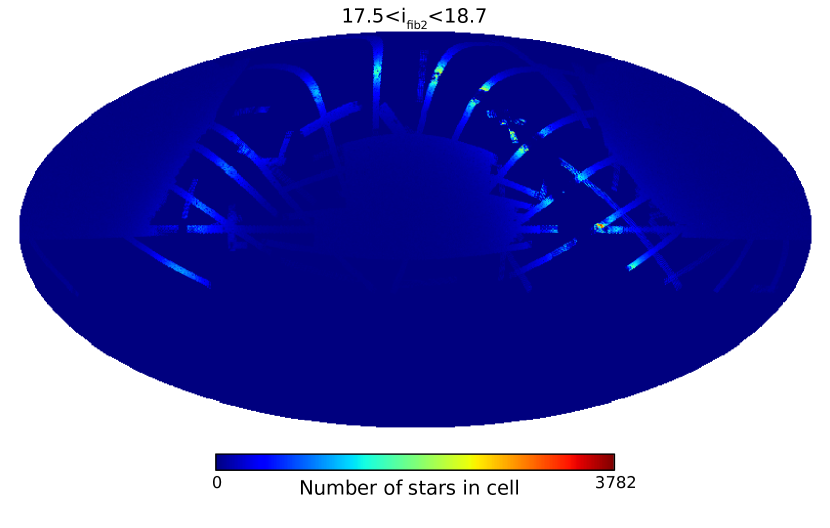
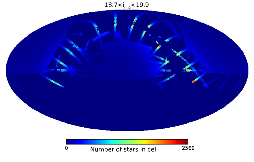
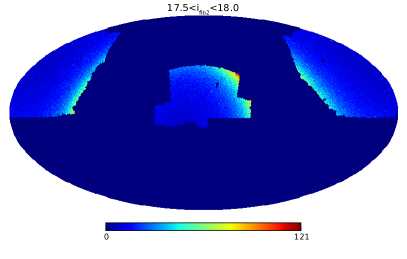
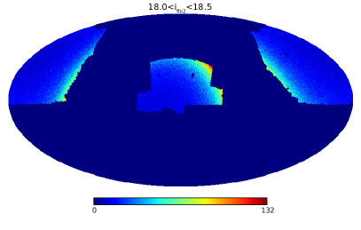
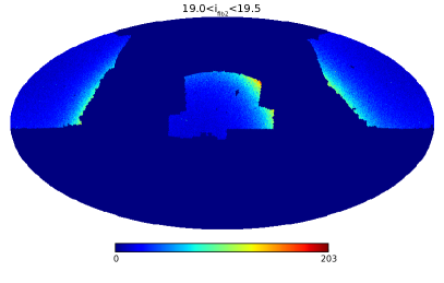
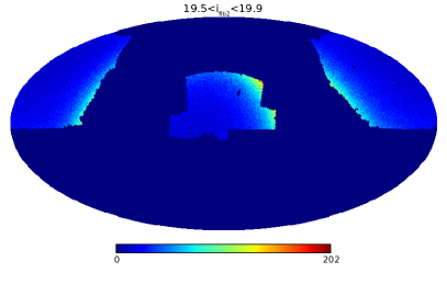
As described in Sec. 2.5, we start by creating a stellar number count map in HEALPix (cf. Fig. 21) of the contaminant which, in this case, we take from the SDSS DR8 star catalogue. Both the BOSS data and the catalogue of stars that we use thus come from the same survey, hence having similar footprints (there are additional stripes running through the Milky Way in the catalogue of stars that are masked out in Fig. 21) and instrumental systematics. The advantage of using HEALPix is that the number count in each pixel is proportional to the angular density of stars, because all pixels cover equally sized areas. Another advantage of HEALPix in general is that the resolution of a map can be easily changed due to the hierarchical ordering of the cells. The resolution can be identified by the “number of pixels per side” ($N_{\mathrm{side}}$), which is related to the total number of pixels on the sphere $N_{\mathrm{pix}}=12N_{\mathrm{side}}^{2}$. The resolution in Fig. 21 is $N_{\mathrm{side}}=256$. Ross et al. (2017) use $N_{\mathrm{side}}=128$ to reduce the shot noise in the stellar data. We reduce the resolution to $N_{\mathrm{side}}=64$, which is sufficient to cover the angular positions of our FKP grid with $128^{3}$ grid points.

The number count and the number density of stars are only proportional to each other in cells that are entirely within the survey footprint. In the original stellar number count map, we could see prominent edge effects, because HEALPix cells on the edges are only partially filled. Considering that each cell has exactly four adjacent cells, we reduce this effect by assuming the following for the completeness of each HEALPix-pixel: pixels in the $N_{\mathrm{side}}=256$-map that have only non-zero neighbours are complete, and for every neighbour that is zero, we assume that the pixel in question is 25 per cent less complete, such that cells, whose neighbours are all empty, are also empty. We generate a HEALPix map with these completeness values and reduce its resolution to $N_{\mathrm{side}}=64$ in the same way as the stellar number count map. We divide the number count of each partially filled pixel by this resulting completeness map, such that we obtain a map whose entries are proportional to the number density of stars.

The objects in the BOSS DR12 CMASS galaxy and random catalogues are assigned to HEALPix cells as described in Sec. 2.5. The randoms are a catalogue of Poisson sampled positions from the expected background density (that is without clustering) under the same spatial selection function as the actual galaxy catalogue. The first step in the creation of the random catalogue is to pick random angular positions distributed according to the completeness of BOSS, which, in a given sector $i$, is estimated as

$$C_{\mathrm{BOSS},i}\equiv\frac{N_{\mathrm{star},i}+N_{\mathrm{gal},i}+N_{\mathrm{fail},i}+N_{\mathrm{cp},i}}{N_{\mathrm{star},i}+N_{\mathrm{gal},i}+N_{\mathrm{fail},i}+N_{\mathrm{cp},i}+N_{\mathrm{missed},i}},$$ (40)

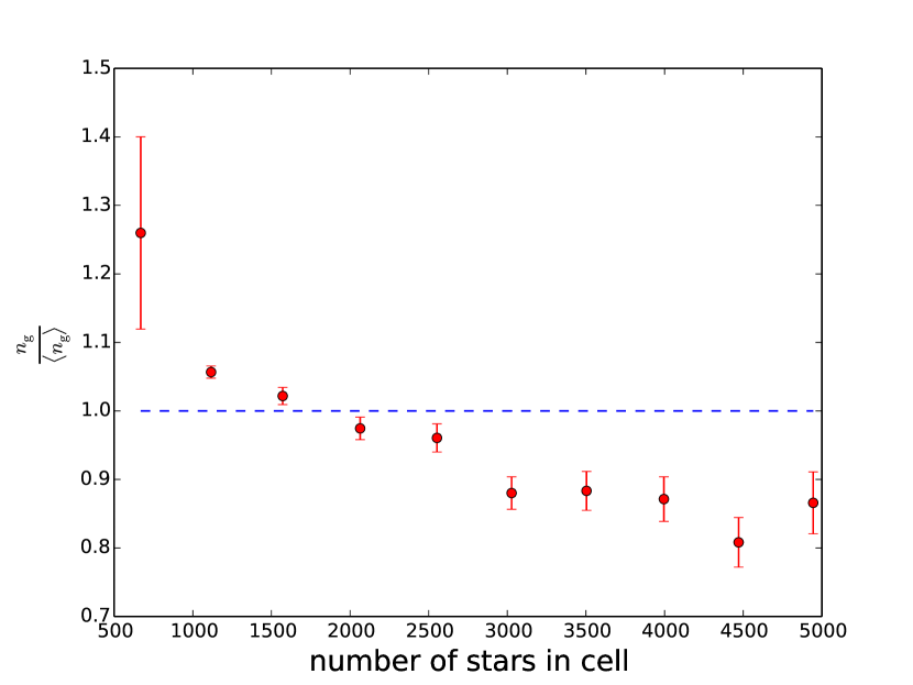
where $N_{\mathrm{star},i}$, $N_{\mathrm{gal},i}$, $N_{\mathrm{fail},i}$, $N_{\mathrm{cp},i}$, $N_{\mathrm{missed},i}$ are the numbers of objects spectroscopically confirmed to be stars, objects that were spectroscopically confirmed a galaxies, objects whose classification failed, close-pair objects of which no spectra could be taken due to fibre collision but with at least one more object in the same target class, and all other objects without spectra (Reid et al., 2016). The next step is to apply veto masks to account for regions where spectra cannot be taken for, e.g., the area around the central bolts of the tiles, the area around targets that have higher targeting priority, areas around bright stars with magnitudes smaller than 11.5. Finally, each object that is still in the random catalogue after vetoing is assigned a random redshift that follows the distribution of the (weighted) galaxies. The random catalogues provided by the BOSS collaboration contain 50 times more random galaxies than there are in the galaxy catalogue. After averaging over all $\frac{n_{\mathrm{g}}}{\langle n_{\mathrm{g}}\rangle}$ in a stellar number count bins, we see a significant deviation from one (cf. Fig. 1), as has been found by Ross et al. (2011, 2017) before. In Fig. 1 we see that in pixels containing less than 1500 stars, we observe more galaxies than we expect from the random catalogue, whereas in pixels with more than 2000 stars, we seem to miss galaxies in the observations.

Figure 1: The average ratio of observed galaxies to expected galaxies from the random catalogue in cells with given numbers of stars.

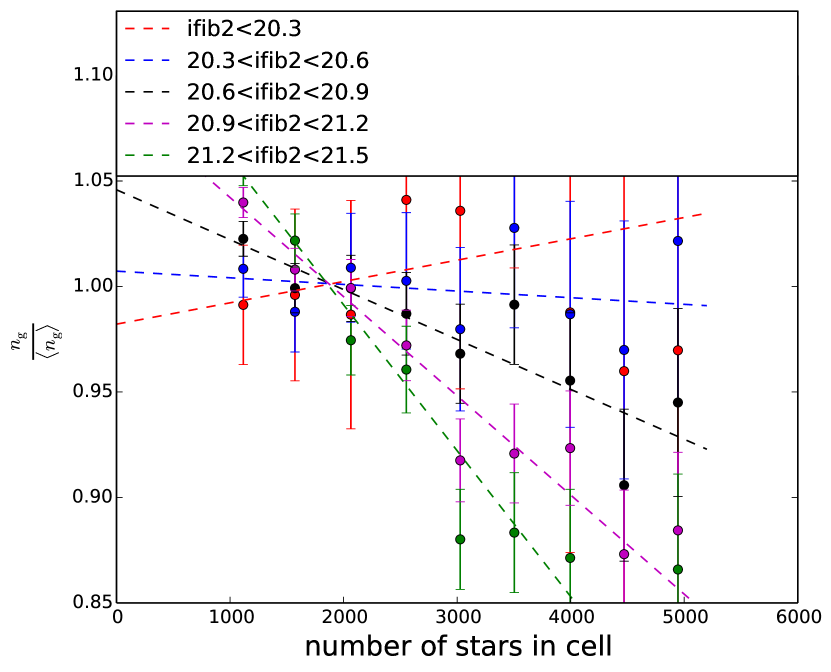
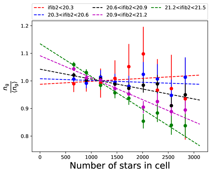
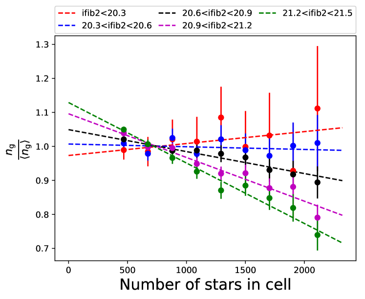
For the effect of obscuration it is reasonable to assume that galaxies with different magnitudes are affected differently by foreground stars. Ross et al. (2013); Ross et al. (2017) therefore made plots similar to Fig. 1, but with the galaxies split into sub-samples by their $i$-band magnitudes within a $2^{\prime\prime}$ aperture radius $i_{\mathrm{fib2}}$. We also follow that procedure to generate Fig. 2, where we can see that galaxy observations are affected very differently according to their surface brightnesses: for galaxies with $i_{\mathrm{fib2}}<20.6$ we see no significant deviation between the expected and observed number of galaxies. For fainter (in terms of surface brightness) galaxies, the best-fitting $\frac{n_{\mathrm{g}}}{\langle n_{\mathrm{g}}\rangle}$-lines are negative and are steeper the larger the galaxies’ magnitudes (i.e. the fainter they are). This meets our expectation, because part of the stellar contamination effect is due to obscuration. To obtain Ross et al. (2017)’s weights for a given galaxy, Eq. (32) is extended by making the fitting coefficients $C_{0}(i_{\mathrm{fib2}})$ and $C_{1}(i_{\mathrm{fib2}})$ magnitude dependent:

$$\frac{n_{\mathrm{g}}}{\langle n_{\mathrm{g}}\rangle}^{(1)}(n_{\mathrm{stars}},i_{\mathrm{fib2}})\equiv C_{0}(i_{\mathrm{fib2}})+C_{1}(i_{\mathrm{fib2}})n_{\mathrm{stars}}.$$ (41)

In Ross et al. (2017), the stellar density weight for the $i$th galaxy in the survey with magnitude $i_{\mathrm{fib2}}$ at right ascension $\alpha_{i}$ and $\delta_{i}$ is obtained by evaluating Eq. (41) at its magnitude and at the number of stars in the pixel where it is situated:

$$w_{i}=\frac{1}{\frac{n_{\mathrm{g}}}{\langle n_{\mathrm{g}}\rangle}^{(1)}(n_{\mathrm{stars}}(\alpha_{i},\delta_{i}),i_{\mathrm{fib2}})}.$$ (42)

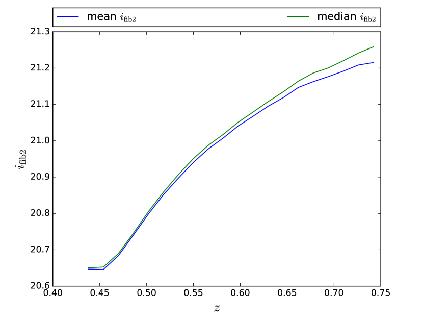
A template based technique, however, requires a field value for $i_{\mathrm{fib2}}$ in either configuration space or Fourier space, so one cannot generate the template using the $i_{\mathrm{fib2}}$-values of individual galaxies. Instead, we average $i_{\mathrm{fib2}}$ in redshift slices (cf. Fig. 3), because farther galaxies tend to have smaller surface brightness, and we assign the averages to template grid cells according to their redshifts. Apart from this, the weights entering Eq. (23) are obtained in the same way as Ross et al. (2017)’s weights:

$$w(\mathbf{x})=w(z,\alpha,\delta)=\frac{1}{\frac{n_{\mathrm{g}}}{\langle n_{\mathrm{g}}\rangle}^{(1)}(n_{\mathrm{stars}}(\alpha,\delta),\langle i_{\mathrm{fib2}}\rangle(z))}.$$ (43)

Figure 2: Plot similar to Fig. 1, but points in different colours are for different subsamples of galaxies with different $i_{\mathrm{fib2}}$ ranges. The dashed lines are the best-fitting lines through the data points.

Figure 3: Mean and median values of the $i_{\mathrm{fib2}}$-magnitudes of BOSS DR12 CMASS galaxies at given redshifts $z$.

Figure 4: The power spectra of the uncorrected BOSS DR12 CMASS NGC galaxies $P_{\mathrm{uncorr}}$ and after 1 to 5 iterations of the debiased mode subtraction procedure, compared to the average power spectrum of the MultiDark-Patchy mocks $P_{\mathrm{Patchy}}$.

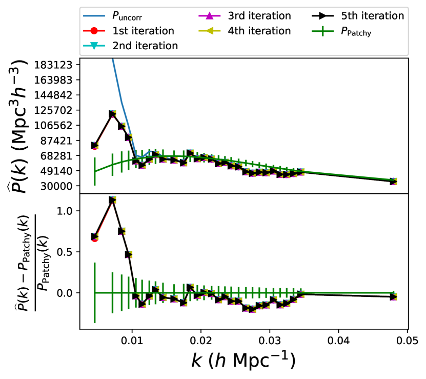
We compute the BOSS DR12 CMASS NGC power spectrum using MOSES. We additionally apply the FKP, fibre-collision, redshift-failure and seeing weights that are provided in the catalogue files. The resulting power spectrum is shown in Fig. 4. We also compute the power spectra of 2048 MultiDark-Patchy mock catalogues (Kitaura et al., 2016) generated using the Perturbation Theory Catalog Generator of Halo and Galaxy Distributions (Kitaura et al., 2015, PATCHY). The mocks are generated using Kitaura et al. (2014)’s Augmented Lagrangian Perturbation Theory and a non-linear bias stochastic scheme. The bias parameters are fitted to the clustering of the BigMultiDark Planck simulation for each redshift snapshot (Klypin et al., 2016). The mass assignment to halos was done with the Halo mAss Distribution ReconstructiON (HADRON) code (Zhao et al., 2015), that takes the local dark matter density, the cosmic web environment and the halo-exclusion effect into account. Finally, light-cones are obtained using the SUrvey GenerAtoR (Rodríguez-Torres et al., 2016, SUGAR) code.

We use the MultiDark-Patchy mock power spectra for three different purposes:

• We estimate the error on our power spectrum measurements as the sample variance of the MultiDark-Patchy power spectra.

• We use the average of the mock power spectra to compare the power spectrum estimates from data against. This has the advantage that the comparison is free of any kind of window effects even though the window changes the large scales a lot.

• We also use the average mock power spectrum as the prior power spectrum needed for MOSES in the debiasing step of Eq. (12).

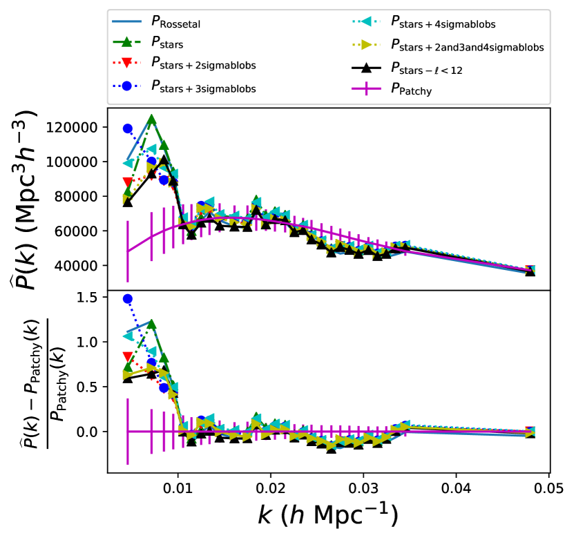
To check the stability of this choice of prior power spectrum, we use, for the first run, the average of the MultiDark-Patchy power spectra as the input prior power spectrum of the error mitigation procedure, and then we iterate by rerunning MOSES with the previous output power spectrum as the prior for the next run. We cannot see any significant difference between the power spectra of the five runs plotted in Fig. 4. Furthermore, all of the five spectra agree well with the power spectrum obtained by mitigating the stellar density contamination using Ross et al. (2017)’s weights (cf. Fig. 4). This shows that MOSES can successfully remove the stellar contamination to first order. On the other hand, we also observe a significant discrepancy between the average MultiDark-Patchy power and our result. One might argue that, due to this discrepancy, the MultiDark-Patchy mocks are not suitable to calculate the covariance of this measurement. However, we are not testing any alternative model to the $\Lambda$CDM model, but any possible deviations from this caused by systematics. Thus, in the absence of any alternative model that we could use to generate a different set of mock catalogues, the errors of the MultiDark-Patchy mocks and their underlying $\Lambda$CDM model describe well the error on our expectation.

3.1.1 Higher Order Stellar Templates

Figure 5: The power spectra of the uncorrected BOSS DR12 CMASS NGC galaxies and after applying debiased mode subtraction with a first order stellar template $P_{1}$, an additional second order template $P_{2}$, and a third order template $P_{3}$. We also show the cases of using one seeing template $P_{3+\mathrm{seeing}}$, and of using 3 airmass templates (first, second and third order) $P_{\mathrm{3+seeing+airmass3}}$. We compare to the average power spectrum of the MultiDark-Patchy mocks.

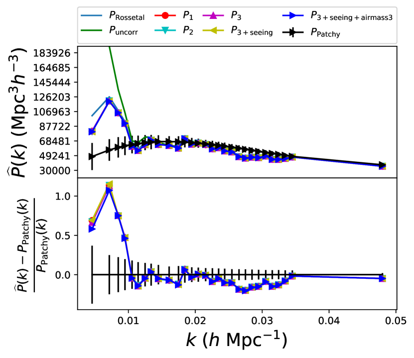
A linear fit is not the only possible relationship between observed galaxies and the number of stars. As discussed in Sec. 2.4, one big advantage of our template based method is that we can add more templates for any form of contamination we have a reason to include. To liberate ourselves from the linear assumption, we follow the steps described in Sec. 2.5 but, as in the previous subsection, we allow for $i_{\mathrm{fib2}}$-dependent fitting coefficients and generate our higher order templates with the redshift dependence of the average magnitude in mind.

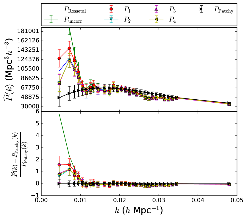
We use Eq. (10) to find the best-fitting amplitude of each template, which are listed in Tab. 1. The amplitude for the first and third order templates, $\varepsilon_{1}^{\mathrm{(BF)}}$ and $\varepsilon_{3}^{\mathrm{(BF)}}$, respectively, do not change significantly when other templates are fitted at the same time. The second order amplitude changes, but it is always at least one order of magnitude less than $\varepsilon_{1}^{\mathrm{(BF)}}$ and $\varepsilon_{3}^{\mathrm{(BF)}}$. The fourth order amplitude $\varepsilon_{4}^{\mathrm{(BF)}}$ is also much smaller, which suggests that the true relationship between observed number of stars and galaxies is an odd function. We compute the debiased mode subtracted power spectra, which we plot in Fig. 5. We observe that, even though $\varepsilon_{3}^{\mathrm{(BF)}}$ is almost as large as $\varepsilon_{1}^{\mathrm{(BF)}}$, including the third order stellar contamination template, or in fact any other higher order template, does not change the resulting power spectrum significantly. This is because the field values of the third order template are two orders of magnitude smaller than those of the first order template. Therefore, for the third order template to have an effect, we would need $\varepsilon_{3}^{\mathrm{(BF)}}\gg\varepsilon_{1}^{\mathrm{(BF)}}$. This is similar for other higher order templates.

Table 1: Best-fitting contamination amplitudes $\varepsilon^{\mathrm{(BF)}}$ for a power spectrum measurement using different numbers of stellar templates.

order	#templates: 1	2	3	4
$1^{\mathrm{st}}$	0.0071	0.0071	0.0072	0.0073
$2^{\mathrm{nd}}$		0.0008	0.0001	0.0008
$3^{\mathrm{rd}}$			0.0055	0.0054
$4^{\mathrm{th}}$				-0.0001

3.1.2 Sub-Sampling the Stars by Magnitude

As the distribution of faint and bright stars is different on the sky, we split the SDSS star catalogue into sub-samples according to the stellar magnitudes.

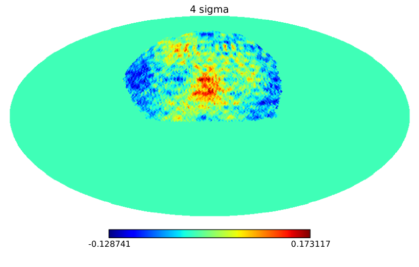
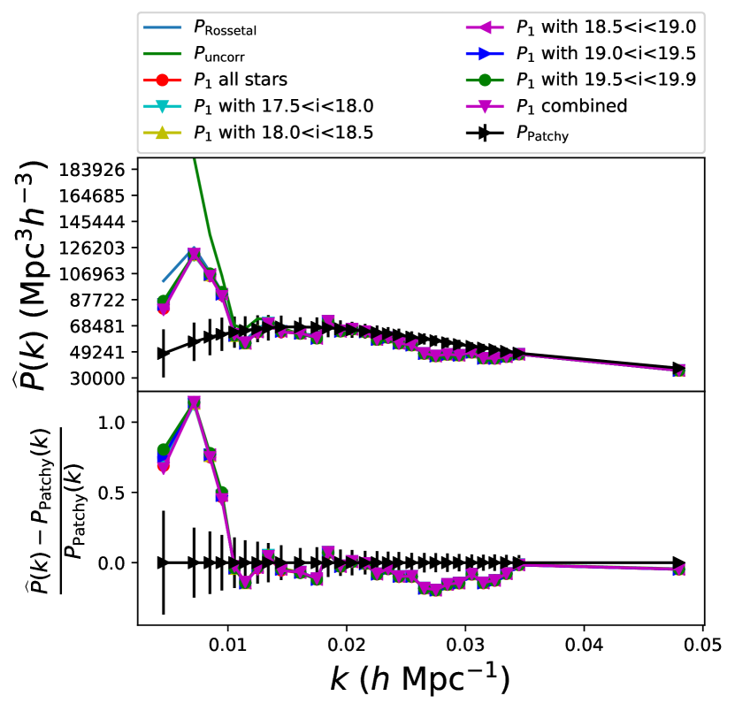
First, we split the star sample into two sub-samples at the central $i$-band magnitude value of $i=18.7$. In Fig. 21 one can see that the two sub-samples also have different spatial distributions: Bright stars are more likely to be found close to the Galactic plane, whereas faint stars are more spread out. The $n_{\mathrm{g}}/\langle n_{\mathrm{g}}\rangle$ diagrams in Fig. 6 do not look very different, though. We refine the magnitude split of the stars and split them into five magnitude bins, each with a width of 0.5, except for the last bin with $19.5<i<19.9$. By comparing the masked maps of each sample (Fig. 22), one can see that the differences in the distribution of stars are only prominent in regions close to the galactic plane from where no galaxies enter BOSS. Therefore, the templates are all strongly correlated, which we can also see in Tab. 2. When fitted separately, all templates have roughly the same amplitude, and each template alone can remove the whole stellar contamination signal, suggesting that they contain mostly the same information. When combined, their amplitudes differ, but the resulting power spectrum does not change. The resulting power spectra are plotted in Fig. 7. We therefore conclude that at different magnitudes, the effect of stars on the galaxy power spectrum is very similar and we therefore do not have to sub-sample the stars by magnitude when mitigating against stellar effects.

Figure 6: The relationship between observed galaxy density and the number of bright stars ($i<18.7$, upper panel) and faint stars ($i>18.7$, lower panel).

Table 2: Best-fitting contamination amplitudes for a power spectrum measurement using five templates for different magnitude ranges of the stars. The values on the left hand side are obtained by fitting only one template at a time, whereas those on the right have been obtained in a simultaneous fit.

magnitude range	separate fit	simultaneous fit
$17.5<i<18.0$	0.007	0.013
$18.0<i<18.5$	0.006	-0.009
$18.5<i<19.0$	0.006	-0.004
$19.0<i<19.5$	0.007	0.009
$19.5<i<19.9$	0.006	-0.003

Figure 7: The power spectra of the uncorrected BOSS DR12 CMASS NGC galaxies (green), and those after mode subtraction using five different templates for stars with different magnitudes, compared to the average power spectrum of the MultiDark-Patchy mocks (black) and the power spectrum using the Ross et al. weights (blue).

3.1.3 Number Count versus Integrated Magnitude

So far, all our stellar templates are based on the number count of stars in regions of the sky. As the effect of the stars is due to their light, this is not the only plausible way of making templates and we explore, as an alternative, basing the templates on the stellar foreground brightness $I(\alpha,\delta)$ in each HEALPix cell. The astronomical magnitude $m$ of an object is defined through the decimal logarithm of its brightness $I$ in units of the brightness of a reference object $I_{\mathrm{ref}}$:

$$m-m_{\mathrm{ref}}\equiv-2.5\log_{10}\left(\frac{I}{I_{\mathrm{ref}}}\right).$$ (44)

Given the $i$-band magnitudes provided in the star catalogue file and used in the previous section, we can obtain the stellar foreground brightness as the sum over the brightness of all stars in a HEALPix cell around the coordinates $(\alpha,\delta)$:

$$I(\alpha,\delta)\propto\sum_{\mathrm{stars\in cell}}10^{-i/2.5}.$$ (45)

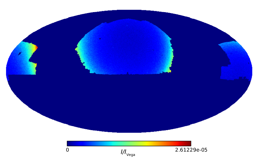
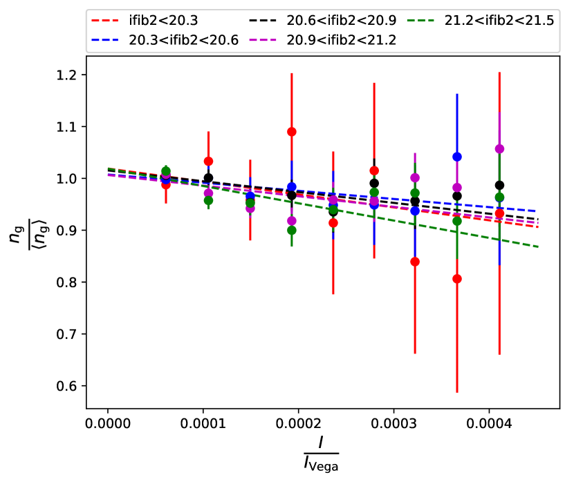
The distribution of the stellar foreground brightness, mapped in Fig. 23, is very similar to the distribution of the number of foreground stars (cf. Fig. 21). However, in Fig. 8 we see that the relationship between observed galaxy density and the foreground brightness $n_{\mathrm{g}}/\langle n_{\mathrm{g}}\rangle(I(\alpha,\delta),i_{\mathrm{fib2}})$ looks very different compared to the same plot for the number counts (cf. Fig. 2), but this can be explained by the fact that the number count and the brightness are approximately logarithmically related. A linear fit does not agree well with the data and the errorbars are so large that we could fit almost any shape with almost any slope. In this case, a more thorough treatment of the error of the template would be needed; however, as the quality of fit of the number count based templates is much better, we leave this for future work.

The first order template for integrated brightness of stars also does worse in removing the contamination than the first order template based on the number counts, as the plot of the resulting power spectrum in Fig. 9 shows. Introducing higher order templates results in power spectra that are similar to the power spectra obtained in the sections before. It shows that the method of introducing templates based on a series expansion of the expected contaminant is working if more than one template is significant, and if they are uncorrelated. On the other hand, it also shows that there is no improvement by constructing the templates on the integrated brightness rather than on the number count of the foreground stars.

Figure 8: The relationship between observed galaxy density and the integrated stellar foreground brightness in units of the brightness of Vega.

Figure 9: Plot similar to Fig. 5 but with templates based on the integrated brightness of stars rather than their number counts.

3.2 Seeing

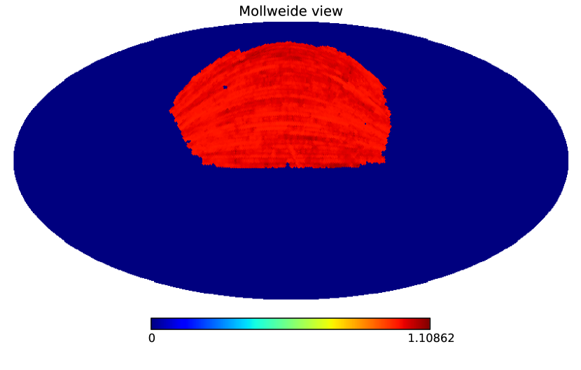
The light travelling to ground based telescopes has to travel through the Earth’s atmosphere. Due to turbulence in the atmosphere, its refractive index changes on short time scales. This blurs the image of an astronomical object and the flux of the object is spread out. This causes an increased magnitude error, and hence, makes it problematic to distinguish between galaxies and stars in the target selection process (Ross et al., 2011), because the star-galaxy separation cut relies entirely on magnitudes. This can cause spurious fluctuations in the observed density field of galaxies (Ross et al., 2011). The seeing can be quantified by measuring the apparent diameter of a point source. In all power spectrum estimates in the previous subsection, we took seeing into account by applying the seeing weights that are provided in the galaxy catalogue file and which are mapped in Fig. 26, which is inconsistent with the way we mitigated against the effects of foreground stars. Here, we use it as a test case of the equivalence of templates and corrective weights that was outlined in Sec. 2.3.

As the effect is purely angular and does not depend on intrinsic properties of the galaxies, we can build our templates by directly inserting Ross et al. (2017)’s weights into Eq. (23). The yellow lines and left facing triangles in Fig. 5 represent the power spectrum we obtained after replacing the direct application of the seeing weights with seeing templates, and using three templates for the stellar contamination. The plot shows that there is no difference between the results obtained using the weights and those obtained using templates based on the same weights. This shows that MOSES works and that the discrepancy between the measured and theoretical power spectra is not due to using different error mitigation techniques inconsistently.

Table 3: Best-fitting contamination amplitudes for a power spectrum measurement using three stellar templates and seeing weights (left) and replacing the seeing weights by seeing templates (right).

template	only stellar	+ 1 seeing template
stars $1^{\mathrm{st}}$ order	0.00719	0.00739
stars $2^{\mathrm{nd}}$ order	0.00009	-0.00002
stars $3^{\mathrm{rd}}$ order	0.00552	0.00576
seeing		-0.00237

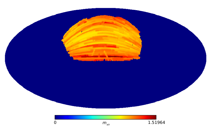
3.3 Airmass

Figure 10: The relationship between observed galaxy density and airmass (cf. Eq. (46)).

Another variation in astronomical observations due to the Earth’s atmosphere arises because light coming from a source close to the horizon has to travel through more atmosphere than the light coming from a source close to the zenith. The effect is quantified by the airmass

$$m_{\mathrm{air}}\equiv\frac{\int\operatorname{d}s\;\rho}{\int\operatorname{d}s_{\mathrm{zenith}}\;\rho},$$ (46)

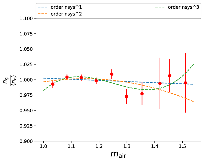
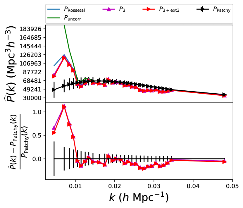
which is the column density, i.e., the integral over the mass density of the atmosphere $\rho$, along the line of sight $s$, divided by the zenith column density. The mass density depends on time-varying quantities such as the temperature and other weather phenomena. Furthermore, the angle between the zenith and the line of sight changes with the seasons. Hence, the amount of photons to be scattered or absorbed varies with both position and observing times, effectively varying the depth of the survey and the magnitude error. Information about the airmass is provided in the random catalogue. A map can be found in Fig. 26. It prominently shows the drift scanning strategy of SDSS. The airmass does not change significantly along SDSS scanning stripes, as the telescope remains stationary along a great circle, but there are sharp leaps from stripe to stripe, which can cause spurious fluctuations in the density field. A plot similar to Fig. 1 that relates $n_{\mathrm{g}}/\langle n_{\mathrm{g}}\rangle$ to the airmass is shown in Fig. 10, where the data points are consistent with $n_{\mathrm{g}}/\langle n_{\mathrm{g}}\rangle=1$ for almost all values of airmass. The linear fit $n_{\mathrm{g}}/\langle n_{\mathrm{g}}\rangle^{\mathrm{(1)}}$ through Fig. 10 is almost constantly equal to one. The quadratic fit $n_{\mathrm{g}}/\langle n_{\mathrm{g}}\rangle^{\mathrm{(2)}}$ shows a slight negative trend at larger airmasses and the cubic fit $n_{\mathrm{g}}/\langle n_{\mathrm{g}}\rangle^{\mathrm{(3)}}$ looks like an over-fit. Ross et al. (2017) made a similar analysis including a $\chi^{2}$ null test. Based on that test, they state that corrections for such a marginally significant effect are ill-advised. However, they recommend to reconsider this choice for any future studies of the clustering of BOSS galaxies at the largest scales.

We proceed as in Sec. 2.5. We fit the three polynomials

$$\frac{n_{\mathrm{g}}}{\langle n_{\mathrm{g}}\rangle}^{(N)}(m_{\mathrm{air}})=\sum_{i=0}^{N}C_{i}m_{\mathrm{air}}^{i}$$ (47)

to the data that we have plotted in Fig. 10. We define

$$E_{\mathrm{am},N}(\alpha,\delta)\equiv\frac{n_{\mathrm{g}}}{\langle n_{\mathrm{g}}\rangle}^{(N)}(m_{\mathrm{air}}(\alpha,\delta))-\frac{n_{\mathrm{g}}}{\langle n_{\mathrm{g}}\rangle}^{(N-1)}(m_{\mathrm{air}}(\alpha,\delta)),$$ (48)

which we insert into Eq. (24) and (30) to obtain templates to mitigate the effect of the airmass.

We perform the mode subtraction method and find the best-fitting template amplitudes given in Tab. 4. The third order template indeed is not favoured by the data and obtains a very small amplitude, suggesting that the third order describes noise rather than an actual effect of the airmass on the observed galaxy density. The first order is almost constant and equal to one, so it cannot be expected to significantly change the resulting power spectrum. The second order template, however, has the largest amplitude coefficient. Yet, including all templates into the power spectrum measurement does only lead to minor corrections in the result, as the blue line in Fig. 5 shows.

Table 4: Best-fitting contamination amplitudes for a power spectrum measurement using three stellar templates (left) and additionally three airmass templates (right).

template	only stellar	+ airmass templates
stars $1^{\mathrm{st}}$ order	0.0072	0.0061
stars $2^{\mathrm{nd}}$ order	0.0001	-0.0013
stars $3^{\mathrm{rd}}$ order	0.0055	0.0042
airmass $1^{\mathrm{st}}$ order		-0.0014
airmass $2^{\mathrm{nd}}$ order		0.0202
airmass $3^{\mathrm{rd}}$ order		-0.0003

3.4 Galactic Extinction

The interstellar medium within our Galaxy causes Galactic Extinction which can be mapped. As blue light is more affected by scattering, extinction causes the light to become redder, and extinction is usually quantified as the difference between the observed (obs) and intrinsic (int) $\mathrm{B-V}$ colour

$$E_{\mathrm{B-V}}=(\mathrm{B-V})_{\mathrm{obs}}-(\mathrm{B-V})_{\mathrm{int}},$$ (49)

where B stands for the filter sensitive to blue light and V is sensitive to visible green-yellow light.

The photometric magnitudes used in the BOSS target selection were corrected using the dust map by Schlegel, Finkbeiner & Davis (1998, SFD). Schlafly & Finkbeiner (2011) found that, using a more accurate reddening law, the SFD map $E_{\mathrm{B-V,SFD}}$ has to be recalibrated such that (Schlafly & Finkbeiner, 2011)

$$E_{\mathrm{B-V}}=0.86E_{\mathrm{B-V,SFD}}.$$ (50)

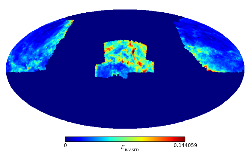
Due to the recalibration, there might be a colour-dependent shift in the target density. A similar $\chi^{2}$ null-test by Ross et al. (2017) led to a similar conclusion as for the airmass test: extinction weights do not significantly change the clustering statistics at BAO scales, but one should be prudent at large scales. For that reason, we test whether including extinction templates changes our power spectrum at large scales. The SFD values of $E_{\mathrm{E-V,SFD}}$ used in the BOSS targeting and listed in the catalogue files are mapped in Fig. 26. There, one can see that extinction mostly affects the SGC part of the BOSS footprint, which we do not analyse in this work. Extinction in NGC occurs mostly in the regions close to the Galactic disk, similar to the stars in Fig. 21. We therefore might expect some correlation between the stellar and extinction templates, as their best-fitting amplitudes $\varepsilon^{\mathrm{(BF)}}$, listed in Tab. 5, also suggest. The amplitudes of the first and third order stellar templates is slightly smaller when fitted at the same time as the extinction templates. The amplitudes of all extinction templates are less than all stellar template amplitudes, explaining why the power spectrum does not change much when extinction templates are included (cf. Fig. 11).

Figure 11: The power spectra of the uncorrected BOSS DR12 CMASS NGC galaxies (green), and those after mode subtraction using 3 stellar templates (magenta) and 3 stellar and 3 extinction templates (red), compared to the average power spectrum of the MultiDark-Patchy mocks (black) and the power spectrum using the Ross et al. weights (blue).

Table 5: Best-fitting contamination amplitudes for a power spectrum measurement using three stellar templates (left) and additionally three extinction templates (right).

template	only stellar	+ extinction templates
stars $1^{\mathrm{st}}$ order	0.0072	0.0070
stars $2^{\mathrm{nd}}$ order	0.0001	0.0023
stars $3^{\mathrm{rd}}$ order	0.0055	0.0043
extinction $1^{\mathrm{st}}$ order		-0.0009
extinction $2^{\mathrm{nd}}$ order		0.0016
extinction $3^{\mathrm{rd}}$ order		0.0020

3.5 Scanning Stripes

Another possible source of data contamination is the instrument itself rather than astronomical or atmospheric foregrounds. For example, the telescope might have a calibration offset between different nights. Furthermore, one can see in Fig. 26 and 26 that time-varying systematics are mostly exposing the drift scanning strategy of SDSS. In fact, Fig. 12 shows that the observed number of galaxies in certain stripes can be significantly different from the number that is expected from the random catalogue.

Figure 12: $n_{\mathrm{g}}/\langle n_{\mathrm{g}}\rangle$ in the different scanning stripes.

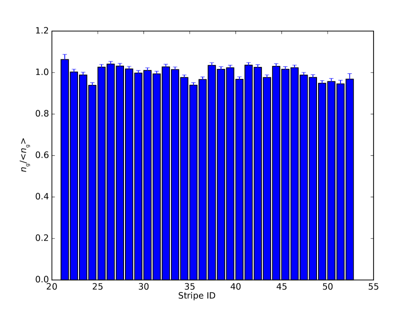
We use Eq. (30) to build templates for each scanning stripe $\eta_{A}$ where everything within the scanning stripe can be mitigated against, but not between stripes, i.e.

$$E_{A}(\mathbf{x})=\begin{cases}1\text{, if }\mathbf{x}\in\eta_{A},\\ 0\text{, else.}\end{cases}$$ (51)

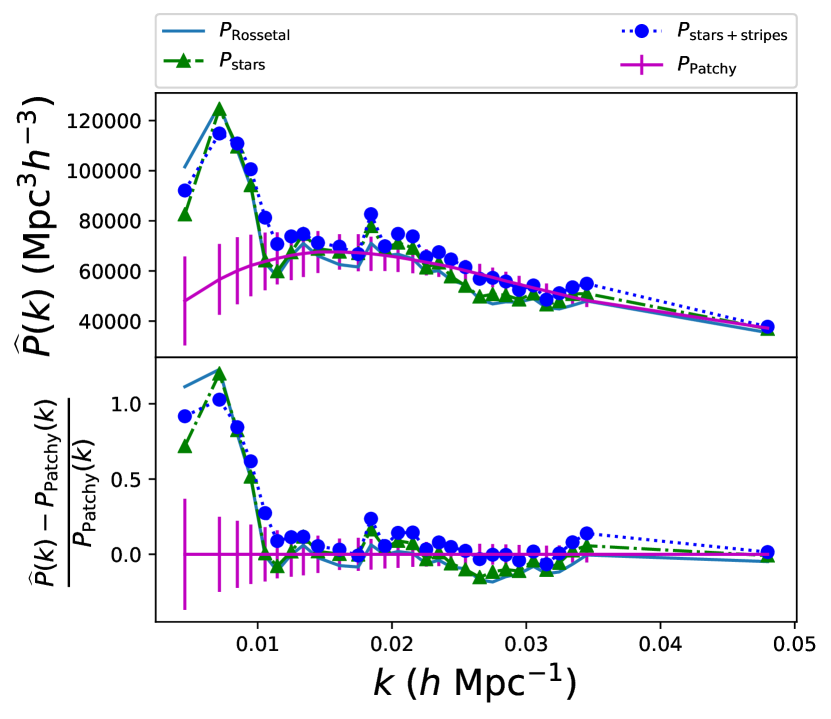
Applying these templates causes a smoothing of the power spectrum (cf. Fig. 13) that can be explained by the fact that the stripe templates affect short scales perpendicular to the scanning stripes and long scales along the stripes. The changes are less than the sample variance of the mock power spectra and therefore leave us with the large scale excess. The stripe templates also remove a dip in the power spectrum compared to the MultiDark-Patchy power spectrum at around $k\approx 0.27\;h\;\mathrm{Mpc}^{-1}$ that is also present e.g. in the power spectrum monopole used for the redshift space distortion measurements by Gil-Marín et al. (2016). Still, most of their signal comes from scales that are not accessible with the coarse grid that we use here, thus, their results are likely to be unaffected by the stripe templates.

Figure 13: Power spectra of BOSS DR 12 CMASS NGC data, using mode subtraction to mitigate the effect of foreground stars (green), as well as stars and possible stripe dependent effects (dotted blue), compared to the power using Ross et al. (2017)’s stellar weights (solid blue) and the average MultiDark-Patchy power spectrum (magenta).

4 Phenomenological Templates

The large-scale offset of the BOSS DR12 CMASS NGC power spectrum compared to what we expect from the MultiDark-Patchy mocks could be due to new or not fully understood physics. However, it is at least as likely instead to be due to unknown systematics. In this Section, we explore phenomenological templates that we generate without any particular source of systematic data contamination in mind.

4.1 Templates Based on Spherical Harmonics Analyses

As most systematics are expected to affect the data only in different angular directions, i.e., not radially, we start with a spherical harmonics decomposition of the data and the mocks. We average the density field along each line-of-sight (LOS) to obtain a density map

$$F_{\mathrm{map}}(\delta,\alpha)\equiv\frac{1}{r_{\mathrm{max}}-r_{\mathrm{min}}}\int_{r_{\mathrm{min}}}^{r_{\mathrm{max}}}\operatorname{d}r\;F(r,\delta,\alpha),$$ (52)

where $F(r,\delta,\alpha)$ is the density field at distance $r$, declination $\delta$ and right ascension $\alpha$. This map can then be decomposed as

$$F_{\mathrm{map}}(\delta,\alpha)=\sum_{\ell=0}^{\infty}\sum_{m=-\ell}^{\ell}a_{\ell m}Y_{\ell m}(\delta,\alpha)$$ (53)

using normalised spherical harmonics $Y_{\ell m}(\delta,\alpha)$ and coefficients $a_{\ell m}$ that we estimate using the HEALPix software package as the following sum over all $N_{\mathrm{pix}}=12N_{\mathrm{side}}^{2}$ HEALPix-pixels (Gorski et al., 2005):

$$a_{\ell m}=\frac{4\pi}{N_{\mathrm{pix}}}\sum_{p=0}^{N_{\mathrm{pix}}-1}Y_{\ell m}^{\ast}(p)F_{\mathrm{map}}(p).$$ (54)

We compute Eq. (54) for both the data (after applying stellar templates) and all MultiDark-Patchy mocks. This allows us to identify multipoles at which the data $a_{\ell m}$ is discrepant with the distribution of the respective mock $a_{\ell m}$. These multipoles are represented by a dot in Fig. 14. At small scales ($\ell\geq 12$), we see that these appear randomly distributed, whereas at large scales ($\ell<12$), we see a large concentration of multipoles that are more than $4\sigma$ away from the expected $a_{\ell m}$ from the MultiDark-Patchy mocks. Interestingly, these are all at positive $m$.

Figure 14: Graphical representation of multipoles $(\ell,m)$ whose measured values of $a_{\ell m}$ is with $2\sigma$ (green), $3\sigma$ (blue) or more than $4\sigma$ (red) discrepant with the average value obtained from MultiDark-Patchy mocks.

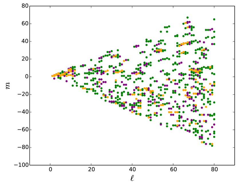
We use the information contained in Fig. 14 to generate our first phenomenological templates: choosing a significance threshold, we do not include multipoles for which the significance of the discrepancy between data and mocks is less than the threshold, but we include the ones exceeding the threshold by inserting

$$E_{A}(z,\alpha,\delta)=\sum_{\ell m\;\mathrm{significant}}\left(a_{\ell m}^{\mathrm{(data)}}-\left\langle a_{\ell m}^{\mathrm{(mocks)}}\right\rangle\right)Y_{\ell m}(\delta,\alpha)$$ (55)

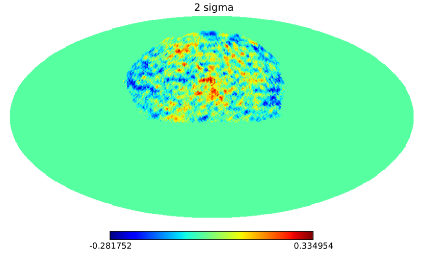
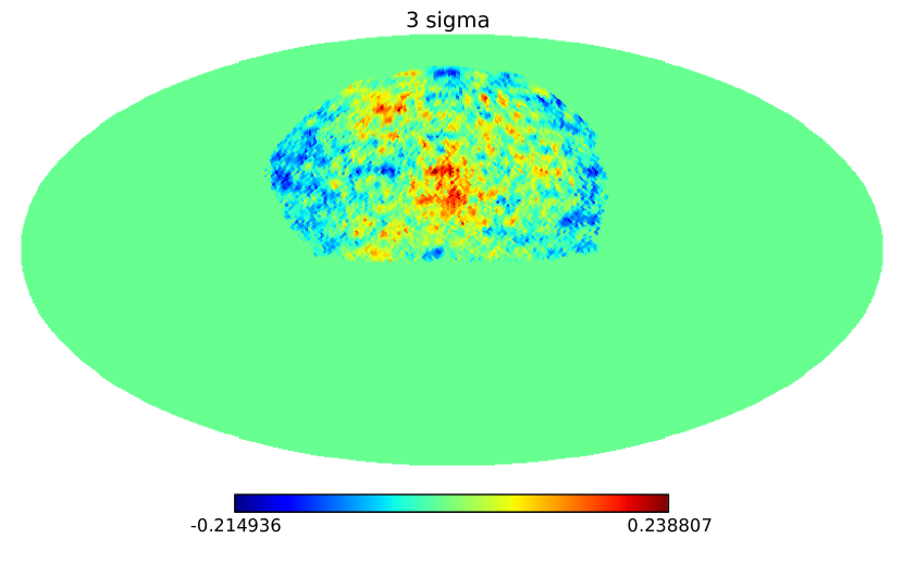
into Eq. (30). Fig. 27 shows the maps corresponding to such a contaminant for a $2\sigma$, $3\sigma$ and $4\sigma$ threshold. All maps show that the centre of the survey footprint is over-dense compared to the mocks. In the $4\sigma$-map, an under-dense ring around the edge becomes more prominent which could be due to unknown galactic effects, or might hint that our treatment of stars could be improved, e.g. by a more thorough treatment of the error on the templates. In Fig. 15, we plot the data power spectrum after applying these phenomenological templates. With the $2\sigma$-template, the power offset in the first two bins halves, but for the $3\sigma$- and $4\sigma$-templates, this is not the case. Applying all 3 phenomenological templates, the power in the first bin is further reduced compared to just applying the $2\sigma$-template, however, in the third bin, we almost see the same power spectrum as if we do not apply the phenomenological templates.

Figure 15: Power spectra of BOSS DR 12 CMASS NGC data, using mode subtraction to mitigate the effect of foreground stars (green), as well as stars and the phenomenological templates of Eq. (55) with a $2\sigma$ (red), $3\sigma$ (blue) or $4\sigma$ (cyan) threshold, as well as all templates combined (yellow), and a template that removes all modes at $\ell<12$. We compare these with the power using Ross et al. (2017)’s stellar weights (solid blue) and to the Patchy power (magenta).

Furthermore, we generate templates

$$E_{A}(z,\alpha,\delta)=\sum_{\ell=0}^{11}\sum_{m=-\ell}^{\ell}\left(a_{\ell m}^{\mathrm{(data)}}-\left\langle a_{\ell m}^{\mathrm{(mocks)}}\right\rangle\right)Y_{\ell m}(\delta,\alpha)$$ (56)

that remove all angular modes at $\ell<12$. Applying this template yields almost the same power spectrum as applying all three previous phenomenological templates. This suggests that something alters the power spectrum along the LOS because Eq. (56) removes all angular modes at multipoles where the data and the mocks are inconsistent with each other. This could be new or not well understood physics, or a new type of unknown systematic, which would require rethinking the common assumption that foregrounds effects are purely angular.

4.2 Cross-correlating Redshift Shells

One can access the information encoded in the radial modes by only considering those modes when computing the power spectrum. In order to not lose information, here we use the projected angular power spectrum of the cross-correlation of non-overlapping redshift bins. Given a wide enough separation between the two subsamples (so that the density correlations are negligible), the only physical correlation arises due to magnification effects. Nonetheless, radial variations in observing conditions or foreground contaminants may also correlate the subsamples. Therefore, in this section we test whether the remaining offset in the power spectrum is a foreground angular contamination, or whether it is a cosmic signal. A foreground contaminant would affect all redshift slices in a similar way and we would therefore see a strong correlation between different shells at the same scales. Therefore, as suggested e.g. by Ho et al. (2012); Pullen & Hirata (2013) and Agarwal et al. (2014), the angular cross power spectrum

$$C_{\ell}^{(xy)}\equiv\frac{1}{2\ell+1}\sum_{m=-\ell}^{\ell}\left(a_{\ell m}^{(x)}\right)^{\ast}a_{\ell m}^{(y)}$$ (57)

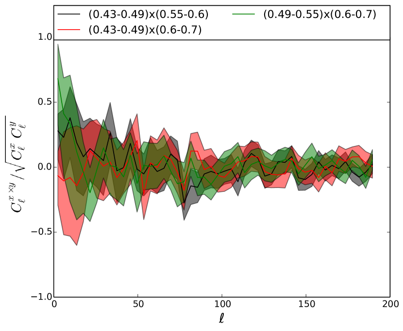
between redshift shells $x$ and $y$ can be used to characterise unknown systematics. In Fig. 16, we quantify cross-correlations between redshift shells by the correlation coefficient

$$C_{\ell}^{(xy)}/\sqrt{C_{\ell}^{(xx)}C_{\ell}^{(yy)}}.$$ (58)

To estimate by-chance correlations, one can do the same cross-correlation studies to the mock catalogues. We choose 4 radial bins in a way that they contain the same number of objects, thus the first bin extends from redshifts of 0.43 to 0.49, the second until 0.55, the third until 0.6 and the fourth up to 0.7. Fig. 16 shows that, as expected, at scales ($\ell\geq 12$), there is no significant cross-correlation between non-adjacent shells. However, the second and fourth shells are strongly correlated at large scales and the first and third only mildly. We do not see any evidence of cross-correlation between the first and fourth shell.

Figure 16: Cross-correlations between BOSS CMASS redshift shells. We applied bandpowering with width $\Delta\ell=4$. The error bars were obtained by cross-correlating the same redshift shells in all MultiDark-Patchy mocks.

Figure 17: Plot similar to Fig. 1 but with the galaxy over-density $\delta_{\mathrm{g}}$ in the redshift shell between $0.49<z<0.55$ as the foreground and considering only galaxies between $0.6<z<0.7$ for $n_{\mathrm{g}}/\langle n_{\mathrm{g}}\rangle$.

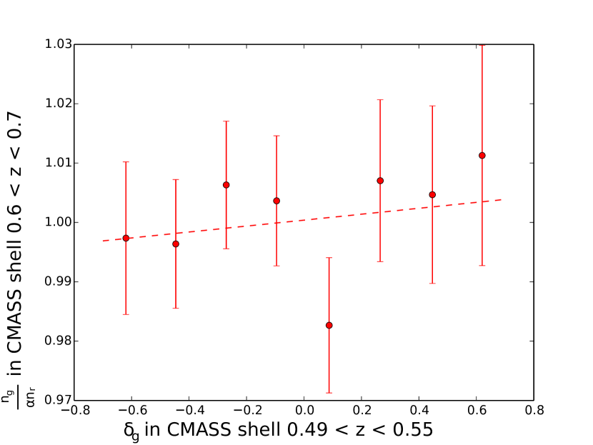
As we saw a strong correlation between the second and fourth radial bins, we test how the ratio of observed versus expected galaxy number density $n_{\mathrm{g}}/\langle n_{\mathrm{g}}\rangle$ in the fourth shell changes with respect to the foreground galaxy over-density $\delta_{\mathrm{g}}$ (cf. Fig. 17). For almost all values of $\delta_{\mathrm{g}}$ in the second bin, we see the expected amount of objects in the fourth bin. A template built in this way is therefore not significantly different from zero and, therefore, does not influence the power spectrum measurement significantly.

4.3 Cross-correlating LOWZ and CMASS

After all the mode subtraction discussed above, we still find no angular contaminant which causes the remaining excess in the measured power spectrum at very large scales with respect to the one computed from the mocks. Surprisingly, the scales at which this excess is located coincide with the largest radial scales of the volume covered by the CMASS catalogue. This is why it is possible that such deviation appears only in radial modes. Therefore, and as we have checked that there is no consistent correlation between different combinations of sub-samples of CMASS separated by redshift, here we test if this excess can be explained with cosmic magnification.

Cosmic magnification due to foreground galaxies affects background galaxy number counts in two competing ways. On one hand, the space behind the lens is stretched, so the background number density decreases. On the other hand, as background sources are magnified, faint galaxies may surpass the detection threshold, which otherwise would have remained undetected. The net effect is then accounted for in the magnification bias, which depends on the specific background sample. Although the magnification signal does not strongly depend on the redshift of the background sources, it may have affected the targeting strategy and contaminate the selection procedure for CMASS, including more galaxies than expected in the faint end of the galaxy population, which is most probably the galaxies with the highest redshifts. Galaxy mocks assume Newtonian gravity but magnification is a relativistic effect, hence we can test if the CMASS sample has a significant amount of magnified galaxies which would not have been targeted otherwise by comparing the cross-correlation of CMASS galaxies with foreground catalogues with the corresponding mocks. In order to avoid the introduction of different assumptions or systematics in this analysis, we choose the BOSS LOWZ sample (spectroscopic as well) as our foreground sample.

Figure 18: Plots similar to Fig. 2 but with the LOWZ over-density field as the foreground. In the top panel, we used the whole LOWZ sample as the foreground, whereas in the bottom panel, only galaxies at redshifts $z<0.29$ have been considered.

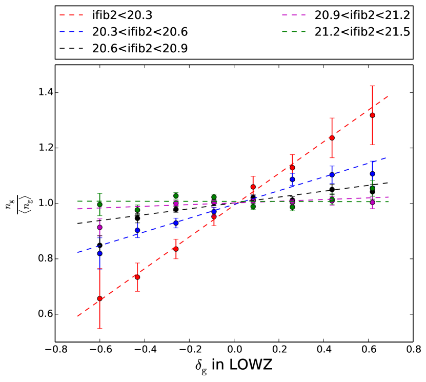
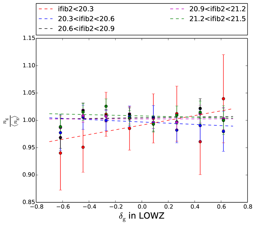
In Fig. 18 we show the ratio between the observed and the expected number counts as function of the number over-density in the LOWZ sample. We split the CMASS data again by $i_{\mathrm{fib2}}$, even though it is regarded as a measure of surface brightness, which is unaffected by lensing. However, as the aperture covers most of the galaxy flux (both before and after it is lensed), $i_{\mathrm{fib2}}$ will catch extra photons from the magnification, i.e. even though surface brightness is conserved, the number of subpixels illuminated by this surface brightness increases. Indeed, we find that significantly fewer very bright galaxies with $i$-fibre magnitudes $i_{\mathrm{fib2}}<20.6$ are observed behind under-dense regions in LOWZ, and significantly more behind over-densities. However, such bright galaxies are rare and have no effect on any template because the average magnitude of even the closest CMASS galaxies (cf. Fig. 3) is fainter than the galaxies showing the effect. Due to their rareness, we also do not see any sizeable effect when applying the classic galaxy-by-galaxy weighting scheme. Moreover, the brightest galaxies in CMASS are the closest ones to us, so it is likely that this positive correlation has a clustering origin rather than being due to magnification. This is further supported by the fact that, if we restrict the LOWZ foreground to $z<0.29$, the cross-correlation is insignificant, suggesting that the significant cross-correlation visible in the top panel of Fig. 18 is due to clustering between LOWZ galaxies at $z>0.29$ and CMASS galaxies at low redshifts.

In order to rule out cosmic magnification as the origin of the excess in the power spectrum, a more comprehensive analysis comparing the results using photometric and spectroscopic catalogues as well as using different galaxy populations as foreground lenses is required. However, this study is beyond the scope of this work and is left for future research.

5 Conclusions

We have presented a practical approach to decontamination using mode subtraction (cf. 2.3 and 2.4). In Sec. 3, we generated templates to mitigate against the effect of foreground stars, seeing, airmass, galactic extinction and the SDSS scanning stripes. We applied these to the final SDSS-III BOSS CMASS NGC sample. We have found that mode subtraction mitigates against systematic contaminants at least as well as deriving and applying corrective weights to the observed objects. As with the corrective weighting, we measure a large-scale excess beyond the power spectrum expected from the standard $\Lambda$CDM cosmology with Gaussian initial density fluctuations. This excess is only present at scales that are much larger than the BAO scale, thus leaving the main results of BOSS unaffected. In Fig. 19, we show that after applying our template based approach the power spectrum is slightly reduced compared to after applying corrective weights. This is because of a small correlation of the observed galaxy density field with the scanning stripes of SDSS, which has previously not been addressed.

Figure 19: Power spectrum of BOSS DR 12 CMASS NGC data after applying weights for all known systematics (stellar density, seeing, airmass, extinction, scanning stripes; to third order where applicable) presented in Sec. 3 (dot-dashed green), as well as after additionally applying the template removing all angular modes at $\ell<12$ (dotted blue). These are compared to the power spectrum we obtain using the same data but applying Ross et al. (2017)’s corrective weights for stars and seeing (solid cyan) and not applying any correction for systematic modes (dashed red). The magenta line represents the average power spectrum of 2049 MultiDark-Patchy realisations.

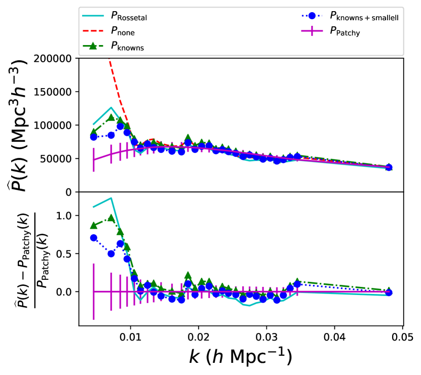
We further tested our methodology by building a range of phenomenological templates. Templates built on a comparison of a spherical harmonics decomposition of the data with the distribution of the decomposed mock catalogue data reduce the large-scale power offset (cf. Section 4.1). However, after applying these phenomenological templates, our large-scale power spectrum measurements are still discrepant with the average mock power spectrum (cf. Fig. 19). Thus, the excess signal is not only coming from angular modes, but there might be a contaminant, or a physical effect, that amplifies the power spectrum along the LOS. The power spectra presented in Fig. 15 and 19 have only been computed to test the Mode Subtraction method; they should not be interpreted as a true measurement, as by using the mock catalogues to generate our templates, we have already partially assumed what we expect.

In Sec. 4.2, we generate further phenomenological templates based on cross-correlations between the CMASS and LOWZ, the other BOSS galaxy sample at lower redshifts, and between redshift shells within the CMASS sample. None of these templates have any sizeable effect on the resulting power spectrum. We therefore do not yet have a satisfactory explanation for the large scale power spectrum excess, which we leave for future work.

In this work, we have shown that MOSES provides power spectrum measurements that are consistent with measurements obtained using corrective weights. The computationally most expensive part of MOSES is the generation of the templates. This is done in the same way that Ross et al. (2017) generate their corrective weights, and when already having weights at hand, Eq. (23) provides a straightforward conversion of the weights into templates. As MOSES is built to ensure an unbiased estimate of the power spectrum, and as one can easily introduce more templates to explore more functional shapes of the contaminant effect, we encourage the use of MOSES.

Appendix A Maps

Figure 20: The distribution of stars in the 8^th SDSS data release in HEALPix. The map is presented in Mollweide projection, equatorial coordinates, astronomical orientation, i.e. east is left, and it has been rotated by $180^{\circ}$ to show the NGC in the centre. The resolution is $N_{\mathrm{side}}=256$. The catalogue includes stars in areas that were not targeted by BOSS. These are masked out in the relevant cells.

Figure 21: Maps of two sub-samples of the SDSS DR8 star catalogue. The upper panel shows the distribution of bright stars with $17.5<i<18.7$ and the lower one faint stars with $18.7<i<19.9$. The plot is in Mollweide projection and in equatorial coordinates with astronomical orientation.

Figure 22: Maps of five sub-samples of the SDSS DR8 star catalogue. The panels show the distribution of stars with $17.5<i<18.0$ (top left), $18.0<i<18.5$ (top right), $18.5<i<19.0$ (centre left), $19.0<i<19.5$ (centre right), and $19.5<i<19.9$ (bottom). The plot is in Mollweide projection and in equatorial coordinates with astronomical orientation.

Figure 23: Map of the brightness distribution of the SDSS DR8 star catalogue. The plot is in Mollweide projection and in equatorial coordinates with astronomical orientation. The map is rotated by $180^{\circ}$ to feature the NGC in the centre. The brightness is given in units of the brightness of the star Vega.

Figure 24: The seeing condition weights of BOSS DR12 CMASS NGC in HEALPix. The map is presented in Mollweide projection, equatorial coordinates and astronomical orientation, but it is rotated by $180^{\circ}$ such that the region observed is in the centre of the map.

Figure 25: The airmass $m_{\mathrm{air}}$ (cf. Eq. 46) in the NGC sub-sample of BOSS DR12 CMASS in HEALPix. The map is presented in Mollweide projection, equatorial coordinates and astronomical orientation, but it is rotated by $180^{\circ}$ such that the region observed is in the centre of the map.

Figure 26: The values of $E_{\mathrm{E-V,SFD}}$ used to correct for extinction in the BOSS targetting in HEALPix. The map is presented in Mollweide projection, equatorial coordinates and astronomical orientation.

Figure 27: Phenomenological “contaminant” maps for a $2\sigma$ (top), $3\sigma$ (centre) and $4\sigma$ (bottom) threshold as defined by Eq. (55) presented in Mollweide projection, equatorial coordinates and astronomical orientation. The maps have been rotated to centre the BOSS NGC footprint. We masked out regions outside of the BOSS NGC footprint since they are unphysical and do not contribute to the templates as the number density of the randoms is zero.

References

- Abazajian et al. (2004) Abazajian K., et al., 2004, Astron. J., 128, 502
- Agarwal et al. (2014) Agarwal N., et al., 2014, JCAP, 1404, 007
- Alam et al. (2015) Alam S., et al., 2015, Astrophys. J. Suppl., 219, 12
- Dawson et al. (2013) Dawson K. S., et al., 2013, Astron. J., 145, 10
- Eisenstein et al. (2011) Eisenstein D. J., et al., 2011, Astron. J., 142, 72
- Elsner et al. (2016) Elsner F., Leistedt B., Peiris H. V., 2016, Mon. Not. Roy. Astron. Soc., 456, 2095
- Elsner et al. (2017) Elsner F., Leistedt B., Peiris H. V., 2017, Mon. Not. Roy. Astron. Soc., 465, 1847
- Feldman et al. (1994) Feldman H. A., Kaiser N., Peacock J. A., 1994, Astrophys. J., 426, 23
- Gil-Marín et al. (2016) Gil-Marín H., et al., 2016, Mon. Not. Roy. Astron. Soc., 460, 4188
- Gorski et al. (2005) Gorski K. M., Hivon E., Banday A. J., Wandelt B. D., Hansen F. K., Reinecke M., Bartelman M., 2005, Astrophys. J., 622, 759
- Gunn et al. (2006) Gunn J. E., et al., 2006, Astron. J., 131, 2332
- Hivon et al. (2002) Hivon E., Gorski K. M., Netterfield C. B., Crill B. P., Prunet S., Hansen F., 2002, Astrophys. J., 567, 2
- Ho et al. (2008) Ho S., Hirata C., Padmanabhan N., Seljak U., Bahcall N., 2008, Phys. Rev., D78, 043519
- Ho et al. (2012) Ho S., et al., 2012, Astrophys. J., 761, 14
- Hunter (2007) Hunter J. D., 2007, Comput. Sci. Eng., 9, 90
- Jasche & Lavaux (2017) Jasche J., Lavaux G., 2017, Astron. Astrophys., 606, A37
- Jasche & Wandelt (2013) Jasche J., Wandelt B. D., 2013, Astrophys. J., 779, 15
- Jasche et al. (2010) Jasche J., Kitaura F. S., Wandelt B. D., Ensslin T. A., 2010, Mon. Not. Roy. Astron. Soc., 406, 60
- Kalus et al. (2016) Kalus B., Percival W. J., Bacon D., Samushia L., 2016, Mon. Not. Roy. Astron. Soc., 463, 467
- Kitaura et al. (2014) Kitaura F.-S., Yepes G., Prada F., 2014, Mon. Not. Roy. Astron. Soc., 439, 21
- Kitaura et al. (2015) Kitaura F.-S., Gil-Marín H., Scoccola C., Chuang C.-H., Müller V., Yepes G., Prada F., 2015, Mon. Not. Roy. Astron. Soc., 450, 1836
- Kitaura et al. (2016) Kitaura F.-S., et al., 2016, Mon. Not. Roy. Astron. Soc., 456, 4156
- Klypin et al. (2016) Klypin A., Yepes G., Gottlober S., Prada F., Hess S., 2016, Mon. Not. Roy. Astron. Soc., 457, 4340
- Leistedt & Peiris (2014) Leistedt B., Peiris H. V., 2014, Mon. Not. Roy. Astron. Soc., 444, 2
- Leistedt et al. (2013) Leistedt B., Peiris H. V., Mortlock D. J., Benoit-Lévy A., Pontzen A., 2013, Mon. Not. Roy. Astron. Soc., 435, 1857
- Leistedt et al. (2014) Leistedt B., Peiris H. V., Roth N., 2014, Phys. Rev. Lett., 113, 221301
- Pullen & Hirata (2010) Pullen A. R., Hirata C. M., 2010, JCAP, 1005, 027
- Pullen & Hirata (2013) Pullen A. R., Hirata C. M., 2013, Publ. Astron. Soc. Pac., 125, 705
- Reid et al. (2016) Reid B., et al., 2016, Mon. Not. Roy. Astron. Soc., 455, 1553
- Rodríguez-Torres et al. (2016) Rodríguez-Torres S. A., et al., 2016, Mon. Not. Roy. Astron. Soc., 460, 1173
- Ross et al. (2011) Ross A. J., et al., 2011, Mon. Not. Roy. Astron. Soc., 417, 1350
- Ross et al. (2013) Ross A. J., et al., 2013, Mon. Not. Roy. Astron. Soc., 428, 1116
- Ross et al. (2017) Ross A. J., et al., 2017, Mon. Not. Roy. Astron. Soc., 464, 1168
- Rybicki & Press (1992) Rybicki G. B., Press W. H., 1992, Astrophys. J., 398, 169
- Schlafly & Finkbeiner (2011) Schlafly E. F., Finkbeiner D. P., 2011, Astrophys. J., 737, 103
- Schlegel et al. (1998) Schlegel D. J., Finkbeiner D. P., Davis M., 1998, Astrophys. J., 500, 525
- Slosar et al. (2004) Slosar A., Seljak U., Makarov A., 2004, Phys. Rev., D69, 123003
- Slosar et al. (2008) Slosar A., Hirata C., Seljak U., Ho S., Padmanabhan N., 2008, JCAP, 0808, 031
- Smee et al. (2013) Smee S., et al., 2013, Astron. J., 146, 32
- Stoughton et al. (2002) Stoughton C., et al., 2002, Astron. J., 123, 485
- Tegmark (1997) Tegmark M., 1997, Phys. Rev., D55, 5895
- Zhao et al. (2015) Zhao C., Kitaura F.-S., Chuang C.-H., Prada F., Yepes G., Tao C., 2015, Mon. Not. Roy. Astron. Soc., 451, 4266