Graph Networks as Learnable Physics Engines for Inference and Control
Supplementary Material: Graph Networks as Learnable Physics Engines for Inference and Control
Abstract
Understanding and interacting with everyday physical scenes requires rich knowledge about the structure of the world, represented either implicitly in a value or policy function, or explicitly in a transition model. Here we introduce a new class of learnable models—based on graph networks—which implement an inductive bias for object- and relation-centric representations of complex, dynamical systems. Our results show that as a forward model, our approach supports accurate predictions from real and simulated data, and surprisingly strong and efficient generalization, across eight distinct physical systems which we varied parametrically and structurally. We also found that our inference model can perform system identification. Our models are also differentiable, and support online planning via gradient-based trajectory optimization, as well as offline policy optimization. Our framework offers new opportunities for harnessing and exploiting rich knowledge about the world, and takes a key step toward building machines with more human-like representations of the world.
1 Introduction
Many domains, such as mathematics, language, and physical systems, are combinatorially complex. The possibilities scale rapidly with the number of elements. For example, a multi-link chain can assume shapes that are exponential in the number of angles each link can take, and a box full of bouncing balls yields trajectories which are exponential in the number of bounces that occur. How can an intelligent agent understand and control such complex systems?
A powerful approach is to represent these systems in terms of objects222“Object” here refers to entities generally, rather than physical objects exclusively. and their relations, applying the same object-wise computations to all objects, and the same relation-wise computations to all interactions. This allows for combinatorial generalization to scenarios never before experienced, whose underlying components and compositional rules are well-understood. For example, particle-based physics engines make the assumption that bodies follow the same dynamics, and interact with each other following similar rules, e.g., via forces, which is how they can simulate limitless scenarios given different initial conditions.
Here we introduce a new approach for learning and controlling complex systems, by implementing a structural inductive bias for object- and relation-centric representations. Our approach uses “graph networks” (GNs), a class of neural networks that can learn functions on graphs (Scarselli et al., 2009b; Li et al., 2015; Battaglia et al., 2016; Gilmer et al., 2017). In a physical system, the GN lets us represent the bodies (objects) with the graph’s nodes and the joints (relations) with its edges. During learning, knowledge about body dynamics is encoded in the GN’s node update function, interaction dynamics are encoded in the edge update function, and global system properties are encoded in the global update function. Learned knowledge is shared across the elements of the system, which supports generalization to new systems composed of the same types of body and joint building blocks.
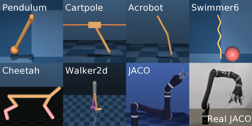
Across seven complex, simulated physical systems, and one real robotic system (see Figure 1), our experimental results show that our GN-based forward models support accurate and generalizable predictions, inference models333We use the term “inference” in the sense of “abductive inference”—roughly, constructing explanations for (possibly partial) observations—and not probabilistic inference, per se. support system identification in which hidden properties are abduced from observations, and control algorithms yield competitive performance against strong baselines. This work represents the first general-purpose, learnable physics engine that can handle complex, 3D physical systems. Unlike classic physics engines, our model has no specific a priori knowledge of physical laws, but instead leverages its object- and relation-centric inductive bias to learn to approximate them via supervised training on current-state/next-state pairs.
Our work makes three technical contributions: GN-based forward models, inference models, and control algorithms. The forward and inference models are based on treating physical systems as graphs and learning about them using GNs. Our control algorithm uses our forward and inference models for planning and policy learning.
(For full algorithm, implementation, and methodological details, as well as videos from all of our experiments, please see the Supplementary Material.)
2 Related Work
Our work draws on several lines of previous research. Cognitive scientists have long pointed to rich generative models as central to perception, reasoning, and decision-making (Craik, 1967; Johnson-Laird, 1980; Miall & Wolpert, 1996; Spelke & Kinzler, 2007; Battaglia et al., 2013). Our core model implementation is based on the broader class of graph neural networks (GNNs) (Scarselli et al., 2005, 2009a, 2009b; Bruna et al., 2013; Li et al., 2015; Henaff et al., 2015; Duvenaud et al., 2015; Dai et al., 2016; Defferrard et al., 2016; Niepert et al., 2016; Kipf & Welling, 2016; Battaglia et al., 2016; Watters et al., 2017; Raposo et al., 2017; Santoro et al., 2017; Bronstein et al., 2017; Gilmer et al., 2017). One of our key contributions is an approach for learning physical dynamics models (Grzeszczuk et al., 1998; Fragkiadaki et al., 2015; Battaglia et al., 2016; Chang et al., 2016; Watters et al., 2017; Ehrhardt et al., 2017; Amos et al., 2018). Our inference model shares similar aims as approaches for learning system identification explicitly (Yu et al., 2017; Peng et al., 2017), learning policies that are robust to hidden property variations (Rajeswaran et al., 2016), and learning exploration strategies in uncertain settings (Schmidhuber, 1991; Sun et al., 2011; Houthooft et al., 2016). We use our learned models for model-based planning in a similar spirit to classic approaches which use pre-defined models (Li & Todorov, 2004; Tassa et al., 2008, 2014), and our work also relates to learning-based approaches for model-based control (Atkeson & Santamaria, 1997; Deisenroth & Rasmussen, 2011; Levine & Abbeel, 2014). We also explore jointly learning a model and policy (Heess et al., 2015; Gu et al., 2016; Nagabandi et al., 2017). Notable recent, concurrent work (Wang et al., 2018) used a GNN to approximate a policy, which complements our use of a related architecture to approximate forward and inference models.
3 Model
Graph representation of a physical system.
Our approach is founded on the idea of representing physical systems as graphs: the bodies and joints correspond to the nodes and edges, respectively, as depicted in Figure 2a. Here a (directed) graph is defined as , where g is a vector of global features, is a set of nodes where each is a vector of node features, and is a set of directed edges where is a vector of edge features, and and are the indices of the sender and receiver nodes, respectively.

We distinguish between static and dynamic properties in a physical scene, which we represent in separate graphs. A static graph contains static information about the parameters of the system, including global parameters (such as the time step, viscosity, gravity, etc.), per body/node parameters (such as mass, inertia tensor, etc.), and per joint/edge parameters (such as joint type and properties, motor type and properties, etc.). A dynamic graph contains information about the instantaneous state of the system. This includes each body/node’s 3D Cartesian position, 4D quaternion orientation, 3D linear velocity, and 3D angular velocity.444Some physics engines, such as Mujoco (Todorov et al., 2012), represent systems using “generalized coordinates”, which sparsely encode degrees of freedom rather than full body states. Generalized coordinates offer advantages such as preventing bodies connected by joints from dislocating (because there is no degree of freedom for such displacement). In our approach, however, such representations do not admit sharing as naturally because there are different input and output representations for a body depending on the system’s constraints. Additionally, it contains the magnitude of the actions applied to the different joints in the corresponding edges.
Graph networks.
The GN architectures introduced here generalize interaction networks (IN) (Battaglia et al., 2016) in several ways. They include global representations and outputs for the state of a system, as well as per-edge outputs. They are defined as “graph2graph” modules (i.e., they map input graphs to output graphs with different edge, node, and global features), which can be composed in deep and recurrent neural network (RNN) configurations. A core GN block (Figure 2b) contains three sub-functions—edge-wise, , node-wise, , and global, —which can be implemented using standard neural networks. Here we use multi-layer perceptrons (MLP). A single feedforward GN pass can be viewed as one step of message-passing on a graph (Gilmer et al., 2017), where is first applied to update all edges, is then applied to update all nodes, and is finally applied to update the global feature. See Algorithm 1 for details.
Forward models.
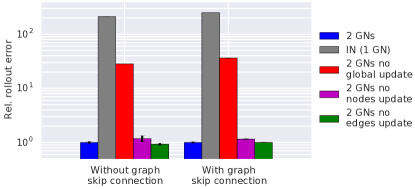
For prediction, we introduce a GN-based forward model for learning to predict future states from current ones. It operates on one time-step, and contains two GNs composed sequentially in a “deep” arrangement (unshared parameters; see Figure 2c). The first GN takes an input graph, , and produces a latent graph, . This is concatenated555We define the term “graph-concatenation” as combining two graphs by concatenating their respective edge, node, and global features. We define “graph-splitting” as splitting the edge, node, and global features of one graph to form two new graphs with the same structure. with (e.g., a graph skip connection), and provided as input to the second GN, which returns an output graph, . Our forward model training optimizes the GN so that ’s features reflect predictions about the states of each body across a time-step. The reason we used two GNs was to allow all nodes and edges to communicate with each other through the output from the first GN. Preliminary tests suggested this provided large performance advantages over a single IN/GN (see ablation study in SM Figure H.2).
We also introduce a second, recurrent GN-based forward model, which contains three RNN sub-modules (GRUs, (Cho et al., 2014)) applied across all edges, nodes, and global features, respectively, before being composed with a GN block (see Figure 2d).
Our forward models were all trained to predict state differences, so to compute absolute state predictions we updated the input state with the predicted state difference. To generate a long-range rollout trajectory, we repeatedly fed absolute state predictions and externally specified control inputs back into the model as input, iteratively. As data pre- and post-processing steps, we normalized the inputs and outputs to the GN model.
Inference models.
System identification refers to inferences about unobserved properties of a dynamic system based on its observed behavior. It is important for controlling systems whose unobserved properties influence the control dynamics. Here we consider “implicit” system identification, in which inferences about unobserved properties are not estimated explicitly, but are expressed in latent representations which are made available to other mechanisms.
We introduce a recurrent GN-based inference model, which observes only the dynamic states of a trajectory and constructs a latent representation of the unobserved, static properties (i.e., performs implicit system identification). It takes as input a sequence of dynamic state graphs, , under some control inputs, and returns an output, , after time steps. This is then passed to a one-step forward model by graph-concatenating it with an input dynamic graph, . The recurrent core takes as input, , and hidden graph, , which are graph-concatenated5 and passed to a GN block (see Figure 2e). The graph returned by the GN block is graph-split5 to form an output, , and updated hidden graph, . The full architecture can be trained jointly, and learns to infer unobserved properties of the system from how the system’s observed features behave, and use them to make more accurate predictions.
Control algorithms.
For control, we exploit the fact that the GN is differentiable to use our learned forward and inference models for model-based planning within a classic, gradient-based trajectory optimization regime, also known as model-predictive control (MPC). We also develop an agent which simultaneously learns a GN-based model and policy function via Stochastic Value Gradients (SVG) (Heess et al., 2015). 666MPC and SVG are deeply connected: in MPC the control inputs are optimized given the initial conditions in a single episode, while in SVG a policy function that maps states to controls is optimized over states experienced during training.
4 Methods
Environments.
Our experiments involved seven actuated Mujoco simulation environments (Figure 1). Six were from the “DeepMind Control Suite” (Tassa et al., 2018)—Pendulum, Cartpole, Acrobot, Swimmer, Cheetah, Walker2d—and one was a model of a JACO commercial robotic arm. We generated training data for our forward models by applying simulated random controls to the systems, and recording the state transitions. We also trained models from recorded trajectories of a real JACO robotic under human control during a stacking task.
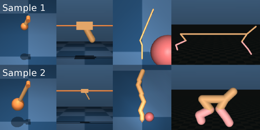
In experiments that examined generalization and system identification, we created a dataset of versions of several of our systems—Pendulum, Cartpole, Swimmer, Cheetah and JACO— with procedurally varied parameters and structure. We varied continuous properties such as link lengths, body masses, and motor gears. In addition, we also varied the number of links in the Swimmer’s structure, from 3-15 (we refer to a swimmer with links as Swimmer).
MPC planning.
We used our GN-based forward model to implement MPC planning by maximizing a dynamic-state-dependent reward along a trajectory from a given initial state. We used our GN forward model to predict the -step trajectories ( is the planning horizon) induced by proposed action sequences, as well as the total reward associated with the trajectory. We optimized these action sequences by backpropagating gradients of the total reward with respect to the actions, and minimizing the negative reward by gradient descent, iteratively.
Model-based reinforcement learning.
To investigate whether our GN-based model can benefit reinforcement learning (RL) algorithms, we used our model within an SVG regime (Heess et al., 2015). The GN forward model was used as a differentiable environment simulator to obtain a gradient of the expected return (predicted based on the next state generated by a GN) with respect to a parameterized, stochastic policy, which was trained jointly with the GN. For our experiments we used a single step prediction (SVG(1)) and compared to sample-efficient model-free RL baselines using either stochastic policies (SVG(0)) or deterministic policies via the Deep Deterministic Policy Gradients (DDPG) algorithm (Lillicrap et al., 2016) (which is also used as a baseline in the MPC experiments).
Baseline comparisons.
As a simple baseline, we compared our forward models’ predictions to a constant prediction baseline, which copied the input state as the output state. We also compared our GN-based forward model with a learned, MLP baseline, which we trained to make forward predictions using the same data as the GN model. We replaced the core GN with an MLP, and flattened and concatenated the graph-structured GN input and target data into a vector suitable for input to the MLP. We swept over 20 unique hyperparameter combinations for the MLP architecture, with up to 9 hidden layers and 512 hidden nodes per layer.
As an MPC baseline, with a pre-specified physical model, we used a Differential Dynamic Programming algorithm (Tassa et al., 2008, 2014) that had access to the ground-truth Mujoco model. We also used the two model-free RL agents mentioned above, SVG(0) and DDPG, as baselines in some tests. Some of the trajectories from a DDPG agent in Swimmer6 were also used to evaluate generalization of the forward models.
Prediction performance evaluation.
Unless otherwise specified, we evaluated our models on squared one-step dynamic state differences (one-step error) and squared trajectory differences (rollout error) between the prediction and the ground truth. We calculated independent errors for position, orientation, linear velocity angular velocity, and normalized them individually to the constant prediction baseline. After normalization, the errors were averaged together. All errors reported are calculated for 1000 100-step sequences from the test set.
5 Results: Prediction
Learning a forward model for a single system.
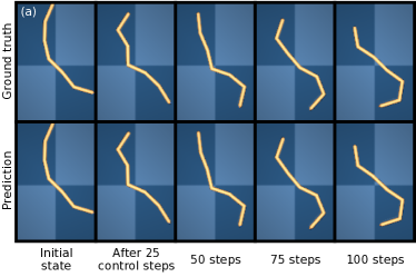
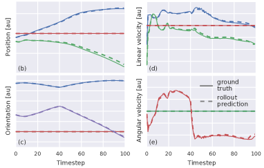
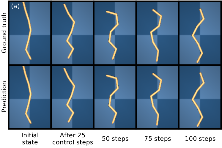
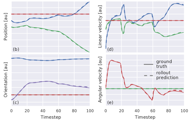
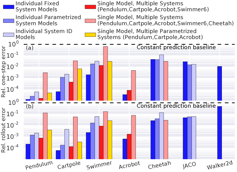
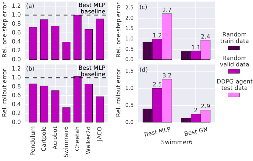
Our results show that the GN-based model can be trained to make very accurate forward predictions under random control. For example, the ground truth and model-predicted trajectories for Swimmer6 were both visually and quantitatively indistinguishable (see Figure 3). Figure 4’s black bars show that the predictions across most other systems were far better than the constant prediction baseline. As a stronger baseline comparison, Figures 5a-b show that our GN model had lower error than the MLP-based model in 6 of the 7 simulated control systems we tested. This was especially pronounced for systems with much repeated structure, such as the Swimmer, while for systems with little repeated structure, such as Pendulum, there was negligible difference between the GN and MLP baseline. These results suggest that a GN-based forward model is very effective at learning predictive dynamics in a diverse range of complex physical systems.
We also found that the GN generalized better than the MLP baseline from training to test data, as well as across different action distributions. Figures 5c-d show that for Swimmer6, the relative increase in error from training to test data, and to data recorded from a learned DDPG agent, was smaller for the GN model than for the MLP baseline. We speculate that the GN’s superior generalization is a result of implicit regularization due to its inductive bias for sharing parameters across all bodies and joints; the MLP, in principle, could devote disjoint subsets of its computations to each body and joint, which might impair generalization.

Learning a forward model for multiple systems.
Another important feature of our GN model is that it is very flexible, able to handle wide variation across a system’s properties, and across systems with different structure. We tested how it learned forward dynamics of systems with continuously varying static parameters, using a new dataset where the underlying systems’ bodies and joints had different masses, body lengths, joint angles, etc. These static state features were provided to the model via the input graphs’ node and edge attributes. Figure 4 shows that the GN model’s forward predictions were again accurate, which suggests it can learn well even when the underlying system properties vary.
We next explored the GN’s inductive bias for body- and joint-centric learning by testing whether a single model can make predictions across multiple systems that vary in their number of bodies and the joint structure. Figure 6 shows that when trained on a mixed dataset of Swimmers with 3-6, 8-9 links, the GN model again learned to make accurate forward predictions. We pushed this even further by training a single GN model on multiple systems, with completely different structures, and found similarly positive results (see Figure 4, red and yellow bars). This highlights a key difference, in terms of general applicability, between GN and MLP models: the GN can naturally operate on variably structured inputs, while the MLP requires fixed-size inputs.
The GN model can even generalize, zero-shot, to systems whose structure was held out during training, as long as they are composed of bodies and joints similar to those seen during training. For the GN model trained on Swimmers with 3-6, 8-9 links, we tested on held-out Swimmers with 7 and 10-15 links. Figure 6 shows that zero-shot generalization performance is very accurate for 7 and 10 link Swimmers, and degrades gradually from 11-15 links. Still, their trajectories are visually very close to the ground truth (video: link-P.F.SN(Z)).
Real robot data.
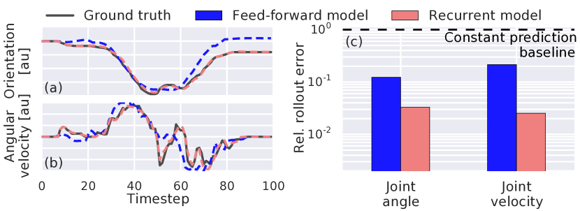
To evaluate our approach’s applicability to the real world, we trained GN-based forward models on real JACO proprioceptive data; under manual control by a human performing a stacking task. We found the feed-forward GN performance was not as accurate as the recurrent GN forward model777This might result from lag or hysteresis which induces long-range temporal dependencies that the feed-forward model cannot capture.: Figure 7 shows a representative predicted trajectory from the test set, as well as overall performance. These results suggest that our GN-based forward model is a promising approach for learning models in real systems.
6 Results: Inference
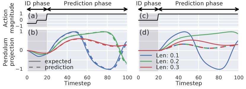
In many real-world settings the system’s state is partially observable. Robot arms often use joint angle and velocity sensors, but other properties such as mass, joint stiffness, etc. are often not directly measurable. We applied our system identification inference model (see Model Section 3) to a setting where only the dynamic state variables (i.e., position, orientation, and linear and angular velocities) were observed, and found it could support accurate forward predictions (during its “prediction phase”) after observing randomly controlled system dynamics during an initial 20-step “ID phase” (see Figure 8).
To further explore the role of our GN-based system identification, we contrasted the model’s predictions after an ID phase, which contained useful control inputs, against an ID phase that did not apply control inputs, across three different Pendulum systems with variable, unobserved lengths. Figure 9 shows that the GN forward model with an identifiable ID phase makes very accurate predictions, but with an unidentifiable ID phase its predictions are very poor.

A key advantage of our system ID approach is that once the ID phase has been performed for some system, the inferred representation can be stored and reused to make trajectory predictions from different initial states of the system. This contrasts with an approach that would use an RNN to both infer the system properties and use them throughout the trajectory, which thus would require identifying the same system from data each time a new trajectory needs to be predicted given different initial conditions.


7 Results: Control
Differentiable models can be valuable for model-based sequential decision-making, and here we explored two approaches for exploiting our GN model in continuous control.
Model-predictive control for single systems.
We trained a GN forward model and used it for MPC by optimizing the control inputs via gradient descent to maximize predicted reward under a known reward function. We found our GN-based MPC could support planning in all of our control systems, across a range of reward functions. For example, Figure 10 shows frames of simulated JACO trajectories matching a target pose and target palm location, respectively, under MPC with a 20-step planning horizon.
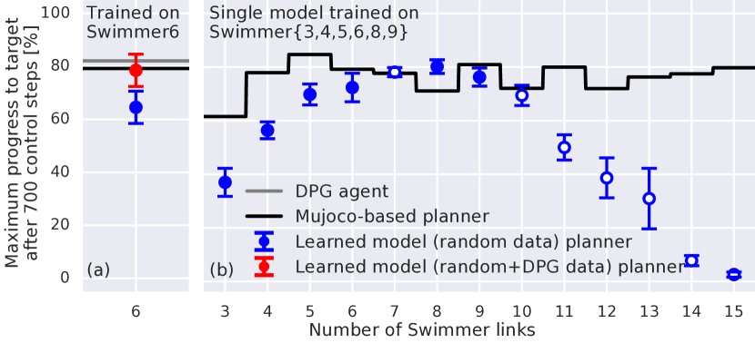
In the Swimmer6 system with a reward function that maximized the head’s movement toward a randomly chosen target, GN-based MPC with a 100-step planning horizon selected control inputs that resulted in coordinated, swimming-like movements. Despite the fact that the Swimmer6 GN model used for MPC was trained to make one-step predictions under random actions, its swimming performance was close to both that of a more sophisticated planning algorithm which used the true Mujoco physics as its model, as well as that of a learned DDPG agent trained on the system (see Figure 11a). And when we trained the GN model using a mixture of both random actions and DDPG agent trajectories, there was effectively no difference in performance between our approach, versus the Mujoco planner and learned DDPG agent baselines (see video: link-C.F.S6).
For Cheetah with reward functions for maximizing forward movement, maximizing height, maximizing squared vertical speed, and maximizing squared angular speed of the torso, MPC with a 20-step horizon using a GN model resulted in running, jumping, and other reasonable patterns of movements (see video: link-C.F.Ch(k)).
Model-predictive control for multiple systems.
Similar to how our forward models learned accurate predictions across multiple systems, we also found they could support MPC across multiple systems (in this video, a single model is used for MPC in Pendulum, Cartpole, Acrobot, Swimmer6 and Cheetah: link-C.F.MS). We also found GN-based MPC could support zero-shot generalization in the control setting, for a single GN model trained on Swimmers with 3-6, 8-9 links, and tested on MPC on Swimmers with 7, 10-15 links. Figure 11b shows that it performed almost as well as the Mujoco baseline for many of the Swimmers.
Model-predictive control with partial observations.
Because real-world control settings are often partially observable, we used the system identification GN model (see Sections 3 and 5) for MPC under partial observations in Pendulum, Cartpole, SwimmerN, Cheetah, and JACO. The model was trained as in the forward prediction experiments, with an ID phase that applied 20 random control inputs to implicitly infer the hidden properties. Our results show that our GN-based forward model with a system identification module is able to control these systems (Cheetah video: link-C.I.Ch. All videos are in SM Table A.2).
Model-based reinforcement learning.
In our second approach to model-based control, we jointly trained a GN model and a policy function using SVG (Heess et al., 2015), where the model was used to backpropagate error gradients to the policy in order to optimize its parameters. Crucially, our SVG agent does not use a pre-trained model, but rather the model and policy were trained simultaneously.888In preliminary experiments, we found little benefit of pre-training the model, though further exploration is warranted. Compared to a model-free agent (SVG(0)), our GN-based SVG agent (SVG(1)) achieved a higher level performance after fewer episodes (Figure 12). For GN-based agents with more than one forward step (SVG(2-4)), however, the performance was not significantly better, and in some cases was worse (SVG(5+)).

8 Discussion
This work introduced a new class of learnable forward and inference models, based on “graph networks” (GN), which implement an object- and relation-centric inductive bias. Across a range of experiments we found that these models are surprisingly accurate, robust, and generalizable when used for prediction, system identification, and planning in challenging, physical systems.
While our GN-based models were most effective in systems with common structure among bodies and joints (e.g., Swimmers), they were less successful when there was not much opportunity for sharing (e.g., Cheetah). Our approach also does not address a common problem for model-based planners that errors compound over long trajectory predictions.
Some key future directions include using our approach for control in real-world settings, supporting simulation-to-real transfer via pre-training models in simulation, extending our models to handle stochastic environments, and performing system identification over the structure of the system as well as the parameters. Our approach may also be useful within imagination-based planning frameworks (Hamrick et al., 2017; Pascanu et al., 2017), as well as integrated architectures with GN-like policies (Wang et al., 2018).
This work takes a key step towards realizing the promise of model-based methods by exploiting compositional representations within a powerful statistical learning framework, and opens new paths for robust, efficient, and general-purpose patterns of reasoning and decision-making.
References
- Amos et al. (2018) Amos, B., Dinh, L., Cabi, S., Rothörl, T., Muldal, A., Erez, T., Tassa, Y., de Freitas, N., and Denil, M. Learning awareness models. ICLR, 2018.
- Atkeson & Santamaria (1997) Atkeson, C. G. and Santamaria, J. C. A comparison of direct and model-based reinforcement learning. In Robotics and Automation, 1997. Proceedings., 1997 IEEE International Conference on, volume 4, pp. 3557–3564. IEEE, 1997.
- Battaglia et al. (2016) Battaglia, P., Pascanu, R., Lai, M., Rezende, D. J., et al. Interaction networks for learning about objects, relations and physics. In NIPS, pp. 4502–4510, 2016.
- Battaglia et al. (2013) Battaglia, P. W., Hamrick, J. B., and Tenenbaum, J. B. Simulation as an engine of physical scene understanding. Proceedings of the National Academy of Sciences, 110(45):18327–18332, 2013.
- Bronstein et al. (2017) Bronstein, M. M., Bruna, J., LeCun, Y., Szlam, A., and Vandergheynst, P. Geometric deep learning: going beyond euclidean data. IEEE Signal Processing Magazine, 34(4):18–42, 2017.
- Bruna et al. (2013) Bruna, J., Zaremba, W., Szlam, A., and LeCun, Y. Spectral networks and locally connected networks on graphs. arXiv preprint arXiv:1312.6203, 2013.
- Chang et al. (2016) Chang, M. B., Ullman, T., Torralba, A., and Tenenbaum, J. B. A compositional object-based approach to learning physical dynamics. arXiv preprint arXiv:1612.00341, 2016.
- Cho et al. (2014) Cho, K., Van Merriënboer, B., Bahdanau, D., and Bengio, Y. On the properties of neural machine translation: Encoder-decoder approaches. arXiv preprint arXiv:1409.1259, 2014.
- Craik (1967) Craik, K. J. W. The nature of explanation, volume 445. CUP Archive, 1967.
- Dai et al. (2016) Dai, H., Dai, B., and Song, L. Discriminative embeddings of latent variable models for structured data. In ICML, pp. 2702–2711, 2016.
- Defferrard et al. (2016) Defferrard, M., Bresson, X., and Vandergheynst, P. Convolutional neural networks on graphs with fast localized spectral filtering. In NIPS, pp. 3844–3852, 2016.
- Deisenroth & Rasmussen (2011) Deisenroth, M. and Rasmussen, C. Pilco: A model-based and data-efficient approach to policy search. In ICML 28, pp. 465–472. Omnipress, 2011.
- Duvenaud et al. (2015) Duvenaud, D. K., Maclaurin, D., Iparraguirre, J., Bombarell, R., Hirzel, T., Aspuru-Guzik, A., and Adams, R. P. Convolutional networks on graphs for learning molecular fingerprints. In NIPS, pp. 2224–2232, 2015.
- Ehrhardt et al. (2017) Ehrhardt, S., Monszpart, A., Mitra, N. J., and Vedaldi, A. Learning a physical long-term predictor. arXiv preprint arXiv:1703.00247, 2017.
- Fragkiadaki et al. (2015) Fragkiadaki, K., Agrawal, P., Levine, S., and Malik, J. Learning visual predictive models of physics for playing billiards. CoRR, abs/1511.07404, 2015.
- Gilmer et al. (2017) Gilmer, J., Schoenholz, S. S., Riley, P. F., Vinyals, O., and Dahl, G. E. Neural message passing for quantum chemistry. In ICML, pp. 1263–1272, 2017.
- Grzeszczuk et al. (1998) Grzeszczuk, R., Terzopoulos, D., and Hinton, G. Neuroanimator: Fast neural network emulation and control of physics-based models. In Proceedings of the 25th annual conference on Computer graphics and interactive techniques, pp. 9–20. ACM, 1998.
- Gu et al. (2016) Gu, S., Lillicrap, T. P., Sutskever, I., and Levine, S. Continuous deep q-learning with model-based acceleration. CoRR, abs/1603.00748, 2016.
- Hamrick et al. (2017) Hamrick, J. B., Ballard, A. J., Pascanu, R., Vinyals, O., Heess, N., and Battaglia, P. W. Metacontrol for adaptive imagination-based optimization. arXiv preprint arXiv:1705.02670, 2017.
- Heess et al. (2015) Heess, N., Wayne, G., Silver, D., Lillicrap, T., Erez, T., and Tassa, Y. Learning continuous control policies by stochastic value gradients. In NIPS, pp. 2944–2952, 2015.
- Henaff et al. (2015) Henaff, M., Bruna, J., and LeCun, Y. Deep convolutional networks on graph-structured data. arXiv preprint arXiv:1506.05163, 2015.
- Houthooft et al. (2016) Houthooft, R., Chen, X., Duan, Y., Schulman, J., Turck, F. D., and Abbeel, P. Curiosity-driven exploration in deep reinforcement learning via bayesian neural networks. CoRR, abs/1605.09674, 2016.
- Johnson-Laird (1980) Johnson-Laird, P. N. Mental models in cognitive science. Cognitive science, 4(1):71–115, 1980.
- Kingma & Welling (2014) Kingma, D. P. and Welling, M. Auto-encoding variational bayes. In ICLR, 2014.
- Kipf & Welling (2016) Kipf, T. N. and Welling, M. Semi-supervised classification with graph convolutional networks. arXiv preprint arXiv:1609.02907, 2016.
- Levine & Abbeel (2014) Levine, S. and Abbeel, P. Learning neural network policies with guided policy search under unknown dynamics. In Ghahramani, Z., Welling, M., Cortes, C., Lawrence, N. D., and Weinberger, K. Q. (eds.), NIPS 27, pp. 1071–1079. Curran Associates, Inc., 2014.
- Li & Todorov (2004) Li, W. and Todorov, E. Iterative linear quadratic regulator design for nonlinear biological movement systems. In ICINCO (1), pp. 222–229, 2004.
- Li et al. (2015) Li, Y., Tarlow, D., Brockschmidt, M., and Zemel, R. Gated graph sequence neural networks. arXiv preprint arXiv:1511.05493, 2015.
- Lillicrap et al. (2016) Lillicrap, T. P., Hunt, J. J., Pritzel, A., Heess, N., Erez, T., Tassa, Y., Silver, D., and Wierstra, D. Continuous control with deep reinforcement learning. In ICLR, 2016.
- Miall & Wolpert (1996) Miall, R. C. and Wolpert, D. M. Forward models for physiological motor control. Neural networks, 9(8):1265–1279, 1996.
- Nagabandi et al. (2017) Nagabandi, A., Kahn, G., Fearing, R. S., and Levine, S. Neural network dynamics for model-based deep reinforcement learning with model-free fine-tuning. arXiv preprint arXiv:1708.02596, 2017.
- Niepert et al. (2016) Niepert, M., Ahmed, M., and Kutzkov, K. Learning convolutional neural networks for graphs. In ICML, pp. 2014–2023, 2016.
- Pascanu et al. (2017) Pascanu, R., Li, Y., Vinyals, O., Heess, N., Buesing, L., Racanière, S., Reichert, D., Weber, T., Wierstra, D., and Battaglia, P. Learning model-based planning from scratch. arXiv preprint arXiv:1707.06170, 2017.
- Peng et al. (2017) Peng, X. B., Andrychowicz, M., Zaremba, W., and Abbeel, P. Sim-to-real transfer of robotic control with dynamics randomization. CoRR, abs/1710.06537, 2017.
- Rajeswaran et al. (2016) Rajeswaran, A., Ghotra, S., Levine, S., and Ravindran, B. Epopt: Learning robust neural network policies using model ensembles. CoRR, abs/1610.01283, 2016.
- Raposo et al. (2017) Raposo, D., Santoro, A., Barrett, D., Pascanu, R., Lillicrap, T., and Battaglia, P. Discovering objects and their relations from entangled scene representations. arXiv preprint arXiv:1702.05068, 2017.
- Rezende et al. (2014) Rezende, D. J., Mohamed, S., and Wierstra, D. Stochastic backpropagation and approximate inference in deep generative models. In ICML 31, 2014.
- Santoro et al. (2017) Santoro, A., Raposo, D., Barrett, D. G., Malinowski, M., Pascanu, R., Battaglia, P., and Lillicrap, T. A simple neural network module for relational reasoning. In NIPS, pp. 4974–4983, 2017.
- Scarselli et al. (2005) Scarselli, F., Yong, S. L., Gori, M., Hagenbuchner, M., Tsoi, A. C., and Maggini, M. Graph neural networks for ranking web pages. In Web Intelligence, 2005. Proceedings. The 2005 IEEE/WIC/ACM International Conference on, pp. 666–672. IEEE, 2005.
- Scarselli et al. (2009a) Scarselli, F., Gori, M., Tsoi, A. C., Hagenbuchner, M., and Monfardini, G. Computational capabilities of graph neural networks. IEEE Transactions on Neural Networks, 20(1):81–102, 2009a.
- Scarselli et al. (2009b) Scarselli, F., Gori, M., Tsoi, A. C., Hagenbuchner, M., and Monfardini, G. The graph neural network model. IEEE Transactions on Neural Networks, 20(1):61–80, 2009b.
- Schmidhuber (1991) Schmidhuber, J. Curious model-building control systems. In Proc. Int. J. Conf. Neural Networks, pp. 1458–1463. IEEE Press, 1991.
- Spelke & Kinzler (2007) Spelke, E. S. and Kinzler, K. D. Core knowledge. Developmental science, 10(1):89–96, 2007.
- Sun et al. (2011) Sun, Y., Gomez, F. J., and Schmidhuber, J. Planning to be surprised: Optimal bayesian exploration in dynamic environments. In AGI, volume 6830 of Lecture Notes in Computer Science, pp. 41–51. Springer, 2011.
- Tassa et al. (2008) Tassa, Y., Erez, T., and Smart, W. D. Receding horizon differential dynamic programming. In NIPS, pp. 1465–1472, 2008.
- Tassa et al. (2014) Tassa, Y., Mansard, N., and Todorov, E. Control-limited differential dynamic programming. In Robotics and Automation (ICRA), 2014 IEEE International Conference on, pp. 1168–1175. IEEE, 2014.
- Tassa et al. (2018) Tassa, Y., Doron, Y., Muldal, A., Erez, T., Li, Y., Casas, D. d. L., Budden, D., Abdolmaleki, A., Merel, J., Lefrancq, A., et al. Deepmind control suite. arXiv preprint arXiv:1801.00690, 2018.
- Todorov et al. (2012) Todorov, E., Erez, T., and Tassa, Y. Mujoco: A physics engine for model-based control. In Intelligent Robots and Systems (IROS), 2012 IEEE/RSJ International Conference on, pp. 5026–5033. IEEE, 2012.
- Wang et al. (2018) Wang, T., Liao, R., Ba, J., and Fidler, S. Nervenet: Learning structured policy with graph neural networks. ICLR, 2018.
- Watters et al. (2017) Watters, N., Zoran, D., Weber, T., Battaglia, P., Pascanu, R., and Tacchetti, A. Visual interaction networks: Learning a physics simulator from video. In NIPS, pp. 4542–4550, 2017.
- Yu et al. (2017) Yu, W., Liu, C. K., and Turk, G. Preparing for the unknown: Learning a universal policy with online system identification. CoRR, abs/1702.02453, 2017.
Appendix A Summary of prediction and control videos
| Fixed | Parametrized | System ID | |
|---|---|---|---|
| Pendulum | link-P.F.Pe | link-P.P.Pe | link-P.I.Pe |
| Cartpole | link-P.F.Ca | link-P.P.Ca | link-P.I.Ca |
| Acrobot | link-P.F.Ac | - | - |
| Swimmer6 | link-P.F.S6 | - | - |
| (eval. DDPG) | link-P.F.S6(D) | - | - |
| SwimmerN | link-P.F.SN | link-P.P.S6 | link-P.I.S6 |
| (zero-shot) | link-P.F.SN(Z) | - | - |
| Cheetah | link-P.F.Ch | link-P.P.Ch | link-P.I.Ch |
| Walker2d | link-P.F.Wa | - | - |
| JACO | link-P.F.JA | link-P.P.JA | link-P.I.JA |
| Multiple systems | link-P.F.MS | link-P.P.MS | - |
| (with cheetah) | link-P.F.MC | - | - |
| Real JACO | link-P.F.JR | - | - |
| Fixed | Parametrized | System ID | |
|---|---|---|---|
| Pendulum (balance) | link-C.F.Pe | link-C.P.Pe | link-C.I.Pe |
| Cartpole (balance) | link-C.F.Ca | link-C.P.Ca | link-C.I.Ca |
| Acrobot (swing up) | link-C.F.Ac | - | - |
| Swimmer6 (reach) | link-C.F.S6 | - | - |
| SwimmerN (reach) | link-C.F.SN | link-C.P.SN | link-C.I.SN |
| ” baseline | link-C.F.SN(b) | - | - |
| Cheetah (move) | link-C.F.Ch(m) | link-C.P.Ch | link-C.I.Ch |
| Cheetah ( rewards) | link-C.F.Ch(k) | - | - |
| Walker2d ( rewards) | link-C.F.Wa(k) | - | - |
| JACO (imitate pose) | link-C.F.JA(o) | link-C.P.JA(o) | link-C.I.JA(o) |
| JACO (imitate palm) | link-C.F.JA(a) | link-C.P.JA(a) | link-C.I.JA(a) |
| Multiple systems | link-C.F.MS | link-C.P.MS | - |
Appendix B Description of the simulated environments
|
Name
(Timestep) |
Number
of bodies (inc. world) |
Generalized
coordinates |
Actions |
Random parametrization999Density of bodies is kept constant for any changes in size.
(relative range of variation, uniformly sampled) |
|---|---|---|---|---|
|
Pendulum
(20 ms) |
2 |
Total: 1
1: angle of pendulum |
1: rotation torque at axis |
Length (0.2-1)
Mass (0.5-3) |
|
Cartpole
(10 ms) |
3 |
Total: 2
1: horizontal position of cart 1: angle of pole |
1: horizontal force to cart |
Mass of cart (0.2-2)
Length of pole (0.3-1) Thickness (0.4-2.2) of pole |
|
Acrobot
(10 ms) |
3 |
Total: 2
2: angle of each of the links angle of pole |
1: rotation force between the links | N/A |
|
SwimmerN
(20 ms) |
N+1 |
Total: N+2
2: 2-d position of head 1: angle of head N-1: angle of rest of links |
N-1: rotation force between the links |
Number of links (3 to 9 links)
Individual lengths of links (0.3-2) Thickness (0.5-5) |
|
Cheetah
(10 ms) |
8 |
Total: 9
2: 2-d position of torso 1: angle of torso 6: thighs, shins and feet angles |
6: rotation force at thighs, shins and feet |
Base angles (-0.1 to 0.1 rad)
Individual lengths of bodies (0.5-2 approx.) Thickness (0.5-2) |
|
Walker2d
(2.5 ms) |
8 |
Total: 9
2: 2-d position of torso 1: angle of torso 6: thighs, leg and feet angles |
6: rotation at hips, knees and ankles | N/A |
|
Jaco
(100 ms) |
10 |
Total: 9
3: angles of coarse joints 3: angles of fine joints 3: angles of fingers |
9: velocity target at each joint |
Individual body masses (0.5-1.5)
Individual motor gears (0.5-1.5). |
Appendix C System data
C.1 Random control
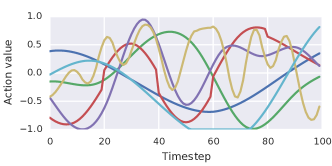
Unless otherwise indicated, we applied random control inputs to the system to generate the training data. The control sequences were randomly selected time steps from spline interpolations of randomly generated values (see SM Figure C.1). A video of the resulting random system trajectories is here: Video.
C.2 Datasets
For each of the individual fixed systems, we generated 10000 100-step sequences corresponding to about supervised training examples. Additionally, we generated 1000 sequences for validation, and 1000 sequences for testing purposes.
In the case of the parametrized environments, we generated 20000 100-step sequences corresponding to about supervised training examples. Additionally, we generated 5000 sequences for validation, and 5000 sequences for testing purposes.
Models trained on multiple environments made use of the corresponding datasets mixed within each batch in equal proportion.
C.3 Real JACO
The real JACO data was obtained under human control during a stacking task. It consisted of 2000 (train:1800, valid:100, test:100) 100-step (timestep 40 ms) trajectories. The instantaneous state of the system was represented in this case by proprioceptive information consisting of joint angles (cosine and sine) and joint velocities for each connected body in the JACO arm, replacing the 13 variables in the dynamic graph.
As the Real JACO observations correspond to the generalized coordinates of the simulated JACO Mujoco model, we use the simulated JACO to render the Real JACO trajectories throughout the paper.
Appendix D Implementation of the models
D.1 Framework
Algorithms were implemented using TensorFlow and Sonnet. We used custom implementations of the graph networks (GNs) as described in the main text.
D.2 Graph network architectures
Standard sizes and output sizes for the GNs used are:
-
•
Edge MLP: 2 or 3 hidden layers. 256 to 512 hidden cells per layer.
-
•
Node and Global MLP: 2 hidden layers. 128 to 256 hidden cells per layer.
-
•
Updated edge, node and global size: 128
-
•
(Recurrent models) Node, global and edge size for state graph: 20
-
•
(Parameter inference) Node, global and edge size for abstract static graph: 10
All internal MLPs used layer-wise ReLU activation functions, except for output layers.
D.3 Data normalization
The two-layer GN core is wrapped by input and output normalization blocks. The input normalization performs linear transformations to produce a zero-mean, unit-variance distributions for each of the global, node and edge features. It is worth noting that for node/edge features, the same transformation is applied to all nodes/edges in the graph, without having specific normalizer parameters for different bodies/edges in the graph. This allows to reuse the same normalizer parameters regardless of the number and type of nodes/edges in the graph. This input normalization is also applied to the observed dynamic graph in the parameter inference network.
Similarly, inverse normalization is applied to the output nodes of the forward model, to guarantee that the network only needs to output nodes with zero-mean and unit-variance.
No normalization is applied to the inferred static graph (from the system identification model), in the output of the parameter inference network, nor the input forward prediction network, as in this case the static graph is already represented in a latent feature space.
D.4 System invariance
When training individual models for systems with translation invariance (Swimmer, Cheetah and Walker2d), we always re-centered the system around 0 before the prediction, and moved it back to its initial location after the prediction. This procedure was not applied when multiple systems were trained together.
D.5 Prediction of dynamic state change
Instead of using the one-step model to predict the absolute dynamic state, we used it to predict the change in dynamic state, which was then used to update the input dynamic state. For the position, linear velocity, and angular velocity, we updated the input by simply adding their corresponding predicted changes. For orientation, where the output represents the rotation quaternion between the input orientation and the next orientation (forced to have unit norm), we computed the update using the Hamilton product.
D.6 Forward prediction algorithms
D.6.1 One-step prediction
Our forward model takes the system parameters, the system state and a set of actions, to produce the next system state as explained in SM Algorithm D.1.
D.6.2 One-step prediction with System ID
For the System ID foward predictions the model takes a system state and a set of actions for a specific instance of a parametrized system, together with a sequence of observed system states and actions for a for the same system instance. The observed sequence is used to identify the system and then produce the next system state as described in Algorithm D.2.
In the case of rollout predictions, the System ID is only performed once, on the provided observed sequence, using the same graph for all of the one-step predictions required to generate the trajectory.
D.7 Training algorithms
D.7.1 One-step
We trained the one-step forward model in a supervised manner using algorithm D.3. Part of the training required finding mean and variance parameters for the input and output normalization, which we did online by accumulating information (count, sum and squared sum) about the distributions of the input edge/node/global features, and the distributions of the change in the dynamic states of the nodes, and using that information to estimate the mean and standard deviation of each of the features.
Due to the fact that our representation of the instantaneous state of the bodies is compatible with configurations where the joint constraints are not satisfied, we need to train our model to always produced outputs within the manifold of configurations allowed by the joints. This was achieved by adding random normal noise (magnitude set as a hyper-parameter) to the nodes of the input dynamic graph during training. As a result, the model not only learns to make dynamic predictions, but to put back together systems that are slightly dislocated, which is key to achieve small rollout errors.
D.7.2 Abstract parameter inference
The training of the parameter inference recurrent GN is performed as described in Algorithm D.4. The recurrent GN and the dynamics GN are trained together end-to-end by sampling a random 20-step sequence for the former, and a random supervised example for the latter from 100-step graph sequences, with a single loss based on the prediction error for the supervised example. This separation between the sequence at the supervised sample, encourages the recurrent GN to truly extract abstract static properties that are independent from the specific 20-step trajectory, but useful for making dynamics predictions under any condition.
D.7.3 Recurrent one-step predictions
The one-step prediction recurrent model, used for the Real JACO predictions, is trained from 21-step sequences using the teacher forcing method. The first 20 graphs in the sequence are used as input graphs, while the last 20 graphs in the sequence are used as target graphs. During training, the recurrent model is used to sequentially process the input graphs, producing at each step a predicted dynamic graph, which is stored, and a graph state, which is fed together with the next input graph in the next iteration. After processing the entire sequence, the sequence of predicted dynamic graphs and the target graphs are used together to calculate the loss.
D.7.4 Loss
We use a standard L2-norm between the normalized expected and predicted delta nodes, for the position, linear velocity, and angular velocity features. We do this for the normalized features to guarantee a balanced relative weighting between the different features. In the case of the orientation, we cannot directly calculate the L2-norm between the predicted rotation quaternion to the expected rotation quaternion , as a quaternion q and represent the same orientation. Instead, we minimize the angle distance between and by minimizing the loss after.
D.8 Training details
Models were trained with a batch size of 200 graphs/graph sequences, using an Adam optimizer on a single GPU. Starting learning rates were tuned at . We used two different exponential decay with factor of 0.975 updated every 50000 (fast training) or 200000 (slow training) steps.
We trained our models using early stopping or asymptotic convergence based the rollout error on 20-step sequences from the validation set. Simple environments (such as individual fixed environments) would typically train using the fast training configuration for a period between less than a day to a few days, depending on the size of the environment and the size of the network. Using slow training in these cases only yields a marginal improvement. On the other hand, more complex models such as those learning multiple environments and multiple parametrized environments benefited from the slow training to achieve optimal behavior for periods of between 1-3 weeks.
Appendix E MLP baseline architectures
For the MLP baselines, we used 5 different models (ReLU activation) spanning a large capacity range:
-
•
3 hidden layers, 128 hidden cells per layer
-
•
3 hidden layers, 512 hidden cells per layer
-
•
9 hidden layers, 128 hidden cells per layer
-
•
9 hidden layers, 512 hidden cells per layer
-
•
5 hidden layers, 256 hidden cells per layer
The corresponding MLP replaces the 2-layer GN core, with additional layers to flatten the input graphs into feature batches, and to reconstruct the graphs at the output. Both normalization and graph update layers are still applied at graph level, in the same way that for the GN-based model.
Each of the models was trained four times using initial learning rates of and and learning rate decays every 50000 and 200000 steps. The model performing best on validation rollouts for each environment, out of the 20 hyperparameter combinations was chosen as the MLP baseline.
Appendix F Control
F.1 Model-based planning algorithms
F.1.1 MPC planner with learned models
We implemented MPC using our learned models as explained in SM Algorithm F.1. We applied the algorithm in a receding horizon manner by iteratively planning for a fixed horizon (see SM Table F.2), applying the first action of the sequence, and increasing the horizon by one step, reusing the shifted optimal trajectory computed in the previous iteration. We typically performed between 3 and 51 optimization iterations from each initial state, with additional iterations at the very first initial state, to warm-up the fully-random initial action sequence.
F.1.2 Baseline Mujoco-based planner
As a baseline planning approach we used the iterative Linear-Quadratic-Gaussian (iLQG) trajectory optimization approach proposed in (Tassa et al., 2014). This method alternates between forward passes (rollouts) which integrate the dynamics forward for a current control sequence and backwards passes which consists of perturbations to the control sequence to improve upon the recursively computed objective function. Note that in the backwards pass, each local perturbation can be formulated as an optimization problem, and linear inequality constraints ensure that the resulting control trajectory does not require controls outside of the range that can be feasibly generated by the corresponding degrees of freedom in the MuJoCo model. The overall objective optimized corresponds to the total cost over a finite horizon:
| (1) |
where is the initial state, is the control signal (i.e. action) taken at timestep , is the trajectory of controls, is the cost function. We assume the dynamics are deterministic transitions .
F.2 Planning configuration
| Name | Task |
Planning
horizon |
Reward to maximize (summed for all timesteps) |
|---|---|---|---|
| Pendulum | Balance | 50, 100 | Negative angle between the quaternion of the pendulum and the target quaternion corresponding to the balanced position. (0 when balanced at the top, otherwise). |
| Cartpole | Balance | 50, 100 | Same as Pendulum-Balance calculated for the pole. |
| Acrobot | Swing up | 100 | Same as Pendulum-Balance summed for both acrobot links. |
| Swimmer | Mover towards target | 100 | Projection of the displacement vector of the Swimmer head from the previous timestep on the target direction, The target direction is calculated as the vector joining the head of the swimmer at the first planning timestep with the target location. The reward is shaped (0.01 contribution) with the negative squared projection on the perpendicular target direction. |
| Cheetah | Move forward | 20 | Horizontal component of the absolute velocity of the torso. |
| Vertical position | 20 | Vertical component of the absolute position of the torso. | |
| Squared vertical speed | 20 | Squared vertical component of the absolute velocity of the torso. | |
| Squared angular speed | 20 | Squared angular velocity of the torso. | |
| Walker2d | Move forward | 20 | Horizontal component of the absolute velocity of the torso. |
| Vertical position | 20 | Vertical component of the absolute position of the torso. | |
| Inverse verticality | 20 | Same as Pendulum-Balance summed for torso, thighs and legs. | |
| Feet to head height | 20 | Summed squared vertical distance between the position of each of the feet and the height of Walker2d. | |
| Jaco | Imitate Palm Pose | 20 | Negative dynamic-state loss (as described in Section D.7.4) between the position-and-orientation of the body representing the JACO palm and the target position-and-orientation . |
| Imitate Full Pose | 20 | Same as Jaco-Imitate Palm Pose but summed across all the bodies forming JACO (see SM Section D.7.4). |
F.3 Reinforcement learning agents
Our RL experiments use three base algorithms for continuous control: DDPG (Lillicrap et al., 2016), SVG(0) and SVG(N) (Heess et al., 2015). All of these algorithms find a policy that selects an action in a given state by maximizing the expected discounted reward,
| (2) |
where is the per-step reward and denotes the discount factor. Learning in all algorithms we consider occurs off-policy. That is, we continuously generate experience via the current best policy , storing all experience (sequences of states, actions and rewards) it into a replay buffer , and minimize a loss defined on samples from via stochastic gradient descent.
F.3.1 DDPG
The DDPG algorithm (Lillicrap et al., 2016) learns a deterministic control policy with parameters and a corresponding action-value function , with parameters . Both of these mapping are parameterized via neural networks in our experiments.
Learning proceeds via gradient descent on two objectives. The objective for learning the function is to minimize the one-step Bellman error using samples from a replay buffer, that is we seek to find by following the gradient,
| (3) | ||||
where and denote the parameters of target Q-value and policy networks, that are periodically copied from the current parameters, this is common practice in RL to stabilize training (we update the target networks every gradient steps). The objective for learning the policy is performed by searching for an action that obtains maximum value, as judged by the learned Q-function. That is we find by following the deterministic policy gradient (Lillicrap et al., 2016),
| (4) |
F.3.2 SVG
For our experiments with the familiy of Stochastic Value Gradient (SVG) (Heess et al., 2015) algorithms we considered two-variants a model-free baseline SVG(0) that optimizes a stochastic policy based on a learned Q-function as well as a model-based version SVG(N) (using our Graph Net model) that unrolls the system dynamics for N-steps.
SVG(0)
In the model-free variant learning proceeds similarly to the DDPG algorithm. We learn both, a parametric Q-value estimator as well as a (now stochastic) policy from which actions can be sampled. In our implementation learning of the Q-function is performed by following the gradient from Equation (3), with replaced by samples .
For the policy learning step we can learn via a stochastic analogue of the deterministic policy gradient from Equation (4), the so called stochastic value gradient, which reads
| (5) |
For a Gaussian policy (as used in this paper) the gradient of this expectation can be calculated via the reparameterization trick (Kingma & Welling, 2014; Rezende et al., 2014).
SVG(N)
For the model based version we used a variation of SVG(N) that employs an action-value function – instead of the value function estimator used in the original paper. This allowed us to directly compare the performance of a SVG(0) agent, which is model free, with SVG(1) which calculates policy gradients using a one-step model based horizon.
In particular, similar to Equation (5), we obtain the model based policy gradient as
| (6) |
where denotes the dynamics, as predicted by the GN and the gradient can, again, be computed via reparameterization (we refer to Heess et al. (2015) for a detailed discussion).
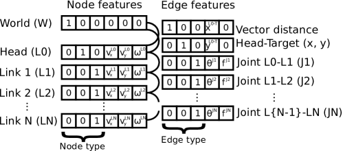
We experimented with SVG(1) on the swimmer domain with six links (Swimmer 6). Since in this case, the goal for the GN is to predict environment observations (as opposed to the full state for each body), we constructed a graph from the observations and actions obtained from the environment. SM Figure H.3 describes the observations and actions and shows how they were transformed into a graph.
Appendix G Mujoco variables included in the graph conversion
G.1 Dynamic graph
We retrieved the the absolute position, orientation, linear and angular velocities for each body:
-
•
Global: None
-
•
Nodes: (for each body)
Absolute body position (3 vars): mjData.xpos
Absolute body quaternion orientation position (4 vars): mjData.xquat
Absolute linear and angular velocity (6 vars): mj_objectVelocity (mjOBJ_XBODY, flg_local=False) -
•
Edges: (for each joint) Magnitude of action at joint: mjData.ctrl (0, if not applicable).
G.2 Static graph
We performed an exhaustive selection of global, body, and joint static properties from mjModel:
-
•
Global: mjModel.opt.{timestep, gravity, wind, magnetic, density, viscosity, impratio, o_margin, o_solref, o_solimp, collision_type (one-hot), enableflags (bit array), disableflags (bit array)}.
-
•
Nodes: (for each body) mjModel.body_{mass, pos, quat, inertia, ipos, iquat}.
-
•
Edges: (for each joint)
Direction of edge (1: parent-to-child, -1: child-to-parent).
Motorized flag (1: if motorized, 0 otherwise).
Joint properties: mjModel.jnt_{type (one-hot), axis, pos, solimp, solref, stiffness, limited, range, margin}.
Actuator properties: mjModel.opt.actuator_{biastype (one-hot), biasprm, cranklength, ctrllimited, ctrlrange, dyntype (one-hot), dynprm, forcelimited, forcerange, gaintype (one-hot), gainprm, gear, invweight0, length0, lengthrange}.
Most of these properties are constant for all environments use, however, they are kept for completeness. While we do not include geom properties such as size, density or shape, this information should be partially encoded in the inertia tensor together with the mass.
Appendix H Supplementary figures
