Theoretical and numerical comparison of hyperelastic and hypoelastic formulations for Eulerian non-linear elastoplasticity

Abstract

The aim of this paper is to compare a hyperelastic with a hypoelastic model describing the Eulerian dynamics of solids in the context of non-linear elastoplastic deformations. Specifically, we consider the well-known hypoelastic Wilkins model, which is compared against a hyperelastic model based on the work of Godunov and Romenski. First, we discuss some general conceptual differences of the two approaches. Second, a detailed study of both models is proposed, where differences are made evident at the aid of deriving a hypoelastic-type model corresponding to the hyperelastic model and a particular equation of state used in this paper. Third, using the same high order ADER Finite Volume and Discontinuous Galerkin methods on fixed and moving unstructured meshes for both models, a wide range of numerical benchmark test problems has been solved. The numerical solutions obtained for the two different models are directly compared with each other. For small elastic deformations, the two models produce very similar solutions that are close to each other. However, if large elastic or elastoplastic deformations occur, the solutions present larger differences.

1 Introduction

Solid dynamics is naturally formulated in Lagrangian coordinates. However, the treatment of excessively large (finite) deformations in the Lagrangian frame is challenging from the computational viewpoint because of the large mesh distortion. Hydrodynamic-type effects like jets and vortexes may appear in many applications involving interactions of solids, e.g. high energetic interactions of metals involving fluidization, melting and solidification in metallurgy, complex flows such as granular flows and flows of viscoplastic fluids (yield stress fluids), which exhibit properties of both elastic solids and viscous fluids [1, 2]. Such hydrodynamic-type effects in solids are naturally treated in the Eulerian settings. It is therefore important to have also a proper Eulerian formulation of solid mechanics, since it is more suitable for treating large deformations. Moreover, an Eulerian formulation is also required for moving mesh techniques based on the Arbitrary Lagrangian Eulerian formulation, see  [19], for example.

In contrast to the Lagrangian frame, in which the description of the dynamics of elastic and plastic solids always relies on the use of strain measures (e.g. deformation gradient) and therefore on a rigorous and objective geometric approach, there are historically two different possibilities to formulate the solid dynamics equations in the Eulerian frame: the hypoelastic and the hyperelastic one. In the hypoelastic-type models the stress tensor plays the role of the thermodynamic state variable along side with the mass, momentum and energy densities, and thus, an evolution equation for the stress tensor is employed (usually for its trace-less part). On the other hand, the hyperelastic Eulerian models, similar to their Lagrangian counterparts, rely on the use of a strain measure as the primary state variable. They are therefore also based on a rigorous geometric description of solid mechanics. The stress tensor in such models is considered merely as the constitutive momentum flux and should be computed from a stress-strain constitutive relation which is completely determined by defining the energy potential. The goal of this paper is to report about the results of a detailed analytical and numerical comparison of two Eulerian models for solid dynamics in the context of nonlinear elastoplastic deformations. In particular, we compare the hypoelastic Wilkins model [170, 105, 98, 57] against the hyperelastic model proposed by Godunov and Romenski in [70, 65, 71] and by Peshkov and Romenski in [126]. Throughout this paper, we will therefore refer to the hyperelastic model as the GPR model.

In this study, we ignore the effects of strain hardening and heat conduction, in order to study only the principal parts of the models, i.e. the evolution of elastic stress and strains and the impact of the terms modeling the inelastic deformations. We also note that the GPR model belongs to the class of so-called rate dependent plasticity models, while the Wilkins model is formulated in the class of ideal (rate-independent) models. Nevertheless, we shall not modify these models in order to make them both either rate-dependent or rate-independent, but we will compare them in the forms as they are mainly used in the literature. We recall that both models, in the forms they are used in this paper, were designed for similar purposes, that is to describe the behavior of metals under high strain-rate loadings. To make such a comparison more informative, we shall run the GPR model with parameters that make its rate-dependent properties less evident.

The structure of the paper is as follows. In Section 2, we discuss the conceptual differences between the hypoelastic and the hyperelastic approach. In Section 3, we elaborate our comparative analysis of the two different models by discussing in detail the differences between their governing partial differential equations. We also derive a hypoelastic-type model that corresponds to the hyperelastic GPR model for a particular equation of state used in this paper. The high order ADER Discontinuous Galerkin (ADER-DG) and finite volume (ADER-FV) schemes employed in this paper are briefly presented in Section 5. In Section 6, we provide the results of the numerical comparison of the approaches on a large test case suite. Finally, we conclude the paper by summarizing the obtained results and discuss further perspectives in Section 7.

2 Conceptual differences between hyperelastic and hypoelastic models

2.1 Lagrangian viewpoint

The Lagrangian viewpoint on the motion of a continuum implies the use of two coordinate systems. The one which labels the material elements, called the Lagrangian coordinate system, will be denoted by $\xi_{a}$, $a=1,2,3$. With respect to the Lagrangian system $\xi_{a}$, the medium is always at rest. The second system of coordinates is a fixed (laboratory) coordinate system, with respect to which the basic characteristics of motion, such as the velocity, displacement, etc. are measured. This fixed coordinate system is called Eulerian coordinate system and will be denoted as $x_{i}$, $i=1,2,3$. The Lagrangian and Eulerian coordinates relate to each other in a one-to-one manner by the laws of motion, e.g. [149],

$$x_{i}=x_{i}(t,\xi_{a}),\qquad\xi_{a}=\xi_{a}(t,x_{i}),$$ (1)

where $t$ is the time.

In the Lagrangian description, the deformation gradient $F_{{i}{a}}\,=\frac{\mathcal{\partial}x_{i}}{\mathcal{\partial}\xi_{a}}$, which contains the full information about the deformation and orientation of the material elements, is used as a primary state variable. The governing equations of motion of an arbitrary continuum (either fluid or solid) can be derived from the Hamilton principle of stationary action [44, 125, 128] and read as

$$\frac{{\rm d}m_{i}}{{\rm d}\,t}-\frac{\mathcal{\partial}U_{F_{{i}{a}}\,}}{\mathcal{\partial}\xi_{a}}=0,\qquad\frac{{\rm d}F_{{i}{a}}\,}{{\rm d}\,t}-\frac{\mathcal{\partial}U_{m_{i}}}{\mathcal{\partial}\xi_{a}}=0,$$ (2)

where ${\rm d}/{\rm d}t=\mathcal{\partial}/\mathcal{\partial}t+v_{k}\mathcal{\partial}/\mathcal{\partial}x_{k}$ is the material time derivative, $m_{i}=\rho_{0}v_{i}$ is the momentum density, $\rho_{0}$ is the reference mass density, $v_{i}=\frac{{\rm d}x_{i}}{{\rm d}\,t}$ is the velocity field, $F_{{i}{a}}\,=\frac{\mathcal{\partial}x_{i}}{\mathcal{\partial}\xi_{a}}$ is the deformation gradient, $U=U(m_{i},F_{ia})$ is the total energy density (including the kinetic energy) of the system, and $U_{m_{i}}=\mathcal{\partial}U/\mathcal{\partial}m_{i}$, $U_{F_{ia}}=\mathcal{\partial}U/\mathcal{\partial}F_{ia}$. It is implied that $U_{m_{i}}=v_{i}$. The energy conservation law

$$\frac{{\rm d}U}{{\rm d}\,t}-\frac{\mathcal{\partial}}{\mathcal{\partial}\xi_{a}}\left(U_{m_{i}}U_{F_{{i}{a}}\,}\right)=0$$ (3)

is the consequence of equations (2), i.e. it can be obtained if (2)₁ is multiplied by $U_{m_{i}}$ and added to (2)₂ multiplied by $U_{F_{{i}{a}}\,}$. Because of the isotropy assumption and the material frame indifference principle, the energy potential $U$ may depend on the deformation gradient only via three invariants of a symmetric strain tensor obtained from $F_{{i}{a}}\,$, e.g. $B_{ab}=F_{{a}{i}}\,F_{{i}{b}}\,$, $a,b=1,2,3$ or ${\bm{B}}={\bm{F}}^{\rm{T}}{\bm{F}}$. Thus, it is implied that

$$U(\bm{m},{\bm{F}})=\tilde{U}(\bm{m},{\bm{B}}).$$ (4)

Note that from the definition of the deformation gradient, it follows that the identity

$$\frac{\mathcal{\partial}F_{{i}{a}}\,}{\mathcal{\partial}\xi_{b}}-\frac{\mathcal{\partial}F_{{i}{b}}\,}{\mathcal{\partial}\xi_{a}}=0,$$ (5)

is fulfilled by the solutions of (2).

We note that in the momentum equation (2)₁, the non-symmetric stress tensor $U_{F_{ia}}$ (the first Piola-Kirchoff stress tensor) is not a state variable but is completely determined by the strains $F_{ia}$ and the specification of the energy potential $U(m_{i},F_{ia})$. In such a formulation, the stress-free equilibrium configuration corresponds to

$$U_{F_{{i}{a}}\,}=0$$ (6)

and is achieved when $F_{{a}{i}}\,F_{{i}{b}}\,=\delta_{ab}$, i.e. when $F_{{i}{a}}\,$ is an orthogonal matrix, or in other words when the length of the line elements ${\rm d}x_{i}$ and ${\rm d}\xi_{a}$ in the current and the reference configurations are equal. This rigorous way of formulating the governing equations in terms of objective geometric quantities is referred to as hyperelastic in the solid dynamics community.

Traditionally, instead of the first-order equations (2) and (3), the well-known second order formulation of solid dynamics with the displacement field as primary variable is typically discretized in computational codes based on the finite element method (FEM). However, in the last decades also the first-order formulation (2), (3) gained some popularity in the context of transient dynamics of solids with the application of finite volume discretizations based on Godunov-type methods [162, 129, 61, 94, 99, 80].

We now discuss how the Lagrangian equations (2) should be generalized in order to take into account also irreversible deformations.

2.2 Inelastic media in the Lagrangian frame

The key feature of inelastic media is their inability to recover the initial state. Such an irreversibility of deformations is due to the microscopic structural changes in the medium. The structural changes mean that the material elements (parcels of molecules) that were attached to each other in space may become disconnected after the irreversible process of material element rearrangements, which is, in fact, the essence of any flow. An obvious consequence of the material element rearrangements is that the real stresses in the medium and the microscopic deformations of material elements always remain finite even though the observable macroscopic deformations encoded in the laws of motion (1) and hence, in the deformation gradient $F_{{i}{a}}\,$, may grow unlimitedly (e.g. in simple shear flow). Another consequence is that the inelastic media might be highly inhomogeneous because at each time instant, in the zone of inelastic deformations, the neighboring material elements might be not connected in the previous time instants and hence may have a history of deformations that is completely independent from each other. The main question is therefore how to describe these facts on the mathematical level.

These ideas can be mathematically expressed as follows. First of all, a local unstressed reference frame is postulated to exist for each material element via a thought experiment [50, 65, 71, 131]. Namely, if an infinitesimal volume is instantaneously cut out of the material and left to relax adiabatically, then it relaxes to a stress-free configuration. Because the material that suffered from inelastic deformations can be highly inhomogeneous, such an unstressed state can not be achieved simultaneously (globally) for all material elements. In other words, the unstressed state is a purely local notion. Therefore, in the local unstressed state, the tangent space at every point of the continuum is assumed to be equipped with an orthonormal basis triad $\bm{\delta}_{\mu}$, $\mu=1,2,3,$ which, in the current deformed state, becomes the triad $\bm{F}^{\rm e}_{{\mu}}\,$ (the superscript 'e' reference to 'elastic' and will be explained later). Mathematically speaking, the linear map $\bm{\delta}_{\mu}\rightarrow\bm{F}^{\rm e}_{{\mu}}\,$, whose components are denoted by $F^{\rm e}_{{i}{\mu}}\,$, $\det(F^{\rm e}_{{i}{\mu}}\,)>0$, defines a local frame in each material point. Eventually, it is assumed that the stresses in the medium are assigned to this local elastic (recoverable) deformation of the material elements $F^{\rm e}_{{i}{\mu}}\,$. Hence, it is natural to assume that the energy $U$ is not a function of $F_{{i}{a}}\,$ but of $F^{\rm e}_{{i}{\mu}}\,$. In addition, because any two invertible matrices $F_{{i}{a}}\,$ and $F^{\rm e}_{{i}{\mu}}\,$ can be related as

$$F_{{i}{a}}\,=F^{\rm e}_{{i}{\mu}}\,F^{\rm p}_{{\mu}{a}}\,$$ (7)

for a certain matrix $F^{\rm p}_{{\mu}{a}}\,$, $\det(F^{\rm p}_{{\mu}{a}}\,)>0$, we assume that

$$\tilde{U}({\bm{F}}^{\rm e})=\tilde{U}({\bm{F}}{\bm{F}}^{\rm-p})=U({\bm{F}},{\bm{F}}^{\rm p}),$$ (8)

where ${\bm{F}}^{\rm-p}$ is the inverse to ${\bm{F}}^{\rm p}$, i.e. $\delta_{ab}=F^{\rm p}_{{a}{\mu}}\,F^{\rm-p}_{{\mu}{b}}\,$, and hence, the Piola-Kirchhoff stress $U_{F_{{i}{a}}\,}$ becomes

$$U_{F_{{i}{a}}\,}=\tilde{U}_{F^{\rm e}_{{i}{\mu}}\,}F^{\rm-p}_{{a}{\mu}}\,,\qquad\text{or}\qquad U_{{\bm{F}}}=\tilde{U}_{{\bm{F}}^{\rm e}}({\bm{F}}^{-\rm p})^{\rm{T}}.$$ (9)

Lee and Liu [100] were among the first to introduce such a decomposition of the deformation gradient $F_{{i}{a}}\,$ into a recoverable (elastic) $F^{\rm e}_{{\mu}{a}}\,$ and irrecoverable (plastic) $F^{\rm p}_{{\mu}{a}}\,$ part. The formula above states a fundamental fact about the Lagrangian description of inelastic deformations, that is one has to know at least two matrices in (7) in order to compute the Lagrangian stress tensor (9). This imposes severe limitations on using a pure Lagrangian approach for modeling very large plastic deformations or fluid flows because, even though the elastic part $F^{\rm e}_{{i}{\mu}}\,$ remains finite, the total deformation gradient $F_{{i}{a}}\,$ and its plastic part $F^{\rm p}_{{\mu}{a}}\,$ potentially may grow unlimitedly and thus, it can be a source of numerical problems and errors. As we shall see later, the situation is quite different in the Eulerian frame. Namely, to compute the Eulerian stress (Cauchy stress), one needs to know only ${\bm{F}}^{\rm e}$, which is always finite.

The full Lagrangian system of governing equations for modeling inelastic deformations can be formulated as follows [61, 97]. It is convenient to chose the vector of state variables as $(\bm{m},{\bm{F}},{\bm{F}}^{\rm p},s)$, where $s$ is the specific entropy. The governing equations are

$$\frac{{\rm d}m_{i}}{{\rm d}\,t}-\frac{\mathcal{\partial}U_{F_{{i}{a}}\,}}{\mathcal{\partial}\xi_{a}}=0,\quad\frac{{\rm d}F_{{i}{a}}\,}{{\rm d}\,t}-\frac{\mathcal{\partial}U_{m_{i}}}{\mathcal{\partial}\xi_{a}}=0,\quad\frac{{\rm d}F^{\rm p}_{{\mu}{a}}\,}{{\rm d}\,t}=-\frac{1}{\theta}U_{F^{\rm p}_{{\mu}{a}}\,},\quad\frac{{\rm d}s}{{\rm d}t}=\frac{1}{\theta U_{s}}U_{F^{\rm p}_{{\mu}{a}}\,}U_{F^{\rm p}_{{\mu}{a}}\,}\geq 0,$$ (10)

where $\theta=\theta({\bm{F}},{\bm{F}}^{\rm p},s)=\tilde{\theta}({\bm{F}}^{\rm e},s)>0$ is a parameter characterizing the rate of strain relaxation, which usually is taken as $\theta\sim\rho_{0}\tau c_{s}^{2}$, where $\rho_{0}$ is the initial density, $c_{s}$ is the shear sound speed, and $\tau$ is the characteristic time of strain relaxation and will be discussed later. The energy potential should be defined as $U(\bm{m},{\bm{F}},{\bm{F}}^{\rm p},s)=\tilde{U}(\bm{m},{\bm{F}}^{\rm e},s)$, where $\tilde{U}$ may depend on ${\bm{F}}^{\rm e}$ only via its invariants. The energy conservation law has the same form as in (3) and still is the consequence of the governing equations (10). It can be obtained as the linear combination of (10) with the coefficients $U_{m_{i}}$, $U_{F_{{i}{a}}\,}$, $U_{F^{\rm p}_{{\mu}{a}}\,}$, and $U_{s}$ for (10)₁, (10)₂, (10)₃, and (10)₄ respectively. A Godunov-type numerical method for equations (10) in the two-dimensional case was constructed in [61].

Given the above considerations, the Lagrangian description of solid mechanics is intrinsically of the hyperelastic type. On the contrary, in the Eulerian framework, we do not have the information about the initial configuration of the continuum and, in particular, about the fields of labels $\xi_{a}$. Nevertheless, the Eulerian evolution equations for the deformation gradient $F_{ia}$ (or its inverse) and its parts $F^{\rm e}_{{i}{\mu}}\,$ and $F^{\rm p}_{{\mu}{a}}\,$ can be easily obtained after the change of variables $\xi_{a}\rightarrow x_{i}$, see e.g. [71, 125]. However, the history of Eulerian solid dynamics took a different route, in which the strain measures were disregarded and the stress tensor was promoted to an independent state variable. This route is the so-called hypoelastic description and is discussed in the following section. Such a choice was motivated by the main interest of the solid dynamics community to formulate a solid dynamics theory capable of dealing with arbitrary finite and even fluid-like irreversible deformations like jets and/or vortexes. Intuitively, one may think that in such cases, any strain-measure-based approach suffers from serious limitations. However, as recently shown in [126, 43, 44, 127], arbitrary motion of a continuum, either solid or fluid, can be successfully described also in the hyperelastic framework, i.e. in a strain-based theory, even for long times and for media undergoing large deformations. This will be discussed later in Section 2.4.

2.3 Hypo-elastic solid dynamics

The hypoelastic approach to solid dynamics was the subject of active research in the 1950ies. Many authors contributed to its development, including Oldroyd [121, 120], Noll [119], Truesdell [163] and Green [74], to name just a few. The theory of hypoelasticity aims to generalize the linear elasticity theory to general flows and large deformations by means of providing a general constitutive relation that is formulated as a time evolution equation relating the rate of stress to the rate of strains. A quite general evolution equation for the stress tensor ${\bm{S}}$ can be found in [120, 74, 119], which constitutes the basis for various hypoelastic models:

$$\frac{{\rm D}{\bm{S}}}{{\rm D}t}=\alpha_{1}\text{tr}(\bm{\Omega})\bm{I}+\alpha_{2}{\bm{S}}+\alpha_{3}\text{tr}(\bm{\Omega}){\bm{S}}+\alpha_{4}\text{tr}({\bm{S}}\bm{\Omega})\bm{I}+\frac{1}{2}\alpha_{5}({\bm{S}}\bm{\Omega}+\bm{\Omega}{\bm{S}})+\alpha_{6}\text{tr}(\bm{\Omega}){\bm{S}}^{2}+\alpha_{7}\text{tr}({\bm{S}}\bm{\Omega}){\bm{S}}+\\ \alpha_{8}\text{tr}({\bm{S}}^{2}\bm{\Omega})\bm{I}+\frac{1}{2}\alpha_{9}({\bm{S}}\bm{\Omega}+\bm{\Omega}{\bm{S}}^{2})+\alpha_{10}\text{tr}({\bm{S}}\bm{\Omega}){\bm{S}}^{2}+\alpha_{11}\text{tr}({\bm{S}}^{2}\bm{\Omega}){\bm{S}}+\alpha_{12}\text{tr}({\bm{S}}^{2}\bm{\Omega}){\bm{S}}^{2}.$$ (11)

Here, $\alpha_{1},\,\alpha_{2},\,\ldots,\,\alpha_{12}$ are regular functions of the three invariants of ${\bm{S}}$, density, and temperature, $\bm{\Omega}=({\bm{L}}-{\bm{L}}^{\rm{T}})/2$, ${\bm{L}}=\nabla{\bm{v}}$, and ${\rm D}/{\rm D}t$ is an objective time derivative. One may immediately notice that the PDE (11) represents a rich source of uncertainties. First of all, the choice of the objective time derivative is fairly arbitrary and not unique, as discussed in [112], for example. It is neither based on a firm physical ground nor on rigorous principles of differential geometry. Moreover, the discretization of these objective stress rates must be performed with great care [105] to ensure that the constitutive law at the discrete level still satisfies the principle of material objectivity. This important property refers to as the incremental objectivity. Let us also note that an objective stress rate such as the Jaumann rate leads to an evolution equation for the stress which cannot be written under conservative form for multi-dimensional flows. This flaw renders the mathematical analysis of discontinuous solutions questionable, as noticed in [58].

The second source of uncertainties is the choice of constitutive functions $\alpha_{i}$, $i=1,2,\ldots,12$ which also cannot be made based on firm physical principles. The functions $\alpha_{i}$ should be specified by means of fitting experimental data. This fitting has to be done in a twelve-dimensional functional space which most likely makes the definition of $\alpha_{i}$ not unique. In practice, as in particular in the Wilkins model considered here, only a few functions (one or two) are considered and usually they are assumed to be constant. However, for large elastic deformations the $\alpha_{i}$ have to depend on the solution, as reported in [93].

We note that the hypoelastic-type models, which usually are obtained from (11) by coupling with proper dissipative terms (usually of the relaxation type), have gained a lot of popularity in non-Newtonian fluid dynamics for modeling viscoelastic and viscoplastic fluids (yield stress fluids), see e.g. [121, 120, 133, 147, 2], in flows of granular media [1, 47], and in non-equilibrium relativistic [115, 85, 155, 103] and non-relativistic [116, 90, 160] gas dynamics, where the stress tensor evolution equation is obtained from the Boltzmann equation by means of the method of moments (such models generalize Maxwell's idea on modeling the viscoelasticity of gases [106, 119]).

We discuss well-posedness and thermodynamics issues of the hypoelastic approach to continuum modeling of flowing media in Section 3.3.5 and 3.3.7. However, we want to emphasize that, in spite of such drawbacks, hypoelastic models are able to reproduce many experimental observations where the data take the form of measurements of changes in stress with respect to changes in strain. That is why they are extensively used by many researchers and engineers and are currently used in many commercial computational codes such as LS-DYNA.

2.4 Hyperelastic Eulerian solid and fluid dynamics

In contrast to the aforementioned hypoelastic formulations, hyperelastic models rely on the direct evolution of a strain measure and thus on a geometric approach. Although the use of a strain-measure might seem to be counter-intuitive for the description of large deformation continuum mechanics (intense plastic deformations, viscous and inviscid fluid flows, etc.), as it was mentioned above, a hyperelastic GPR formulation of fluid and solid dynamics can nevertheless be also applied to model arbitrary fluid flows and solids undergoing large deformations. In what follows, we review the history of Eulerian hyperelastic-type models, not exhaustively though, with applications to inelastic deformations of solids and to fluid flows and we discuss the main features of such models.

The main obstacle of the Lagrangian description of arbitrarily large inelastic deformations is the necessity to use two strain measures for computing the Lagrangian stress tensor $U_{F_{{i}{\mu}}\,}=\tilde{U}_{F^{\rm e}_{{i}{\mu}}\,}F^{\rm-p}_{{a}{\mu}}\,$ (the first Piola-Kirchhoff stress), as discussed in Section 2.2. Thus, the key difference between the Eulerian and the Lagrangian formulations of continuum mechanics, which makes the practical use of Eulerian hyperelastic formulations possible for arbitrary flows, is that the Eulerian description, in principle, relies on the use of only one strain measure, namely the elastic strain $F^{\rm e}_{{\mu}{i}}\,$. This is sufficient to compute the Eulerian stress tensor (i.e. the Cauchy stress), as will be clarified in what follows.

Perhaps, Eckart [50] was the first to propose the idea of using an elastic (recoverable) strain measure in Eulerian inelasticity. In particular, he introduced the notion of the local relaxed state (exactly as discussed in Section 2.2) and suggested to characterize the deviation from this state by the non-Euclidean (i.e. with non-vanishing curvature) metric tensor $g_{ij}$ with the evolution equation

$$\frac{{\rm d}g_{ij}}{{\rm d}\,t}+g_{ik}\frac{\mathcal{\partial}v_{k}}{\mathcal{\partial}x_{j}}+g_{kj}\frac{\mathcal{\partial}v_{k}}{\mathcal{\partial}x_{i}}=-M_{ijkl}E_{g_{kl}},$$ (12)

where $E$ is the specific energy of the system, $E_{g_{kl}}=\mathcal{\partial}E/\mathcal{\partial}g_{kl}$, and $M_{ijkl}E_{g_{ij}}E_{g_{kl}}$ is a positive definite quadratic form which was not specified in [50]. The right-hand side represents the rate of change of the metric tensor due to the microscopic process of structural relaxation and not due to the macroscopic motion of the continuum. Equation (12) was derived based on the first and second laws of thermodynamics. In the same thermodynamics spirit, the concept of the local relaxed state was later discussed by Sedov in [149], who also suggested to use the metric tensor as a thermodynamic state variable. The next important contribution to the Eulerian description of nonlinear inelastic deformation was made by Besseling [12], see also the book [13]. In contrast to Eckart and Sedov, Besseling suggested to use not the metric tensor $g_{ij}$ but a non symmetric strain $b_{\mu i}$ (in notations of [12]) that is related to the metric tensor as $g_{ij}=b_{\mu i}b_{\mu j}$ and is defined as a transformation of the line elements ${\rm d}x_{i}$ in the current deformed state and ${\rm d}a_{\mu}$ in the local relaxed reference state, i.e. ${\rm d}a_{\mu}=b_{\mu i}{\rm d}x_{i}$. As it is clear now, Besseling's $b_{\mu i}$ is exactly the elastic distortion field in the GPR model proposed by Godunov and Romenski [70, 65, 140, 49, 71] and Peshkov and Romenski [126] and further denoted by $A_{{\mu}{i}}\,$, as in our previous papers [126, 43, 44, 19], and which is governed by the evolution equation

$$\frac{{\rm d}A_{{\mu}{i}}\,}{{\rm d}\,t}+A_{{\mu}{j}}\,\frac{\mathcal{\partial}v_{j}}{\mathcal{\partial}x_{i}}=-\frac{1}{\theta(\tau)}E_{A_{{\mu}{i}}\,},$$ (13)

which can be recast into the form

$$\frac{\mathcal{\partial}A_{{\mu}{i}}\,}{\mathcal{\partial}t}+\frac{\mathcal{\partial}(A_{{\mu}{j}}\,v_{j})}{\mathcal{\partial}x_{i}}+v_{j}\left(\frac{\mathcal{\partial}A_{{\mu}{i}}\,}{\mathcal{\partial}x_{j}}-\frac{\mathcal{\partial}A_{{\mu}{j}}\,}{\mathcal{\partial}x_{i}}\right)=-\dfrac{E_{A_{{\mu}{i}}\,}}{\theta(\tau)},$$ (14)

where $E_{A_{{\mu}{i}}\,}=\mathcal{\partial}E/\mathcal{\partial}A_{{\mu}{i}}\,$, and $\theta(\tau)>0$ is a positive function of the strain relaxation time $\tau$ and $E$ is the total energy potential. Originally, Godunov and Romenski presented their model [70] also in terms of the metric tensor $g_{ij}$ (effective metric tensor), while later [65, 140], they started to use the elastic distortion $A_{{\mu}{i}}\,$ as the primary state variable. One of the main motivations for such a model was the deformation of metals at high strain rates, which may exhibit hydrodynamic effects in the case of welding, see e.g. [59]. Another important motivation was to obtain a mathematically well-posed system of equations that can be solved numerically. In particular, they require that the system of governing equations is hyperbolic, and if possible even symmetric hyperbolic. As it has become clear soon, the use of the metric tensor $g_{ij}$ as the elastic strain measure of deviation from the local relaxed state does not lead to a symmetric hyperbolic model. On the other hand, the use of the elastic distortion does allow to symmetrize the model, see [49, 62, 72, 71]. We also note the works by Leonov [101, 102], who, similar to Eckart [50], Sedov [149] and Godunov and Romenski [70], proposed a relaxation model in the context of non-Newtonian polymeric fluids that also employs only the metric tensor $g_{ij}$ as elastic strain measure and as primary thermodynamic state variable, and does not use any other additional total or plastic strain measures.

The dissipative effect due to the inelastic deformations in the GPR formulation was introduced as a relaxation source term (right hand side in (13)) in the evolution equation for the elastic distortion (see further details in Section 3.2). Such a treatment of inelastic deformations attributes the GPR model to rate-dependent plasticity models with the relaxation parameter $\tau$ being the characteristic time of relaxation of tangential strains. Interpolation formulas for $\tau$ for metals at high strain-rates were studied in [66, 67]. Those take into account also the temperature effect and melting. In this paper, we use a simplified version of the dependence of $\tau$ on the state variables, which does not take into account the temperature effect. The shock structure in a relaxed medium modeled with the GPR model was studied in [69, 65, 71]. In the 1980ies, the GPR model was intensively studied numerically by means of a Godunov-type method in works of Merzhievsky and Resnyansky  [107, 110, 108, 111, 109], including one-dimensional and two-dimensional simulations of high-velocity impacts of metals with a moving mesh technique. The linearized version of the GPR model was also extended to modeling of anisotropic composite viscoelastic media in papers by Resnyanski, Romenski and co-authors, e.g.  [134, 144]. The question of hyperbolicity of the GPR formulation for Eulerian non-linear elasticity was studied in [138, 62, 72, 60, 71, 71]. Relations between the hyperelastic and hypoelastic formulations for Eulerian non-linear elasticity was investigated by Romenski in [137].

Independently of the aforementioned references, an Eulerian approach to finite-strain inelasticity was also developed by Plohr and Sharp in [130, 131] in the 1990ies and was implemented in computational codes based on Godunov-type finite volume methods in [161, 168, 114]. In contrast to the GPR formulation of Eulerian inelasticity, which is based on the use of only one strain measure, namely the elastic distortion field, the Plohr-Sharp formulation employs two strains, the total deformation gradient $F_{{i}{a}}\,$ and the plastic strain $F^{\rm p}_{{\mu}{a}}\,$, which measures the change of the line elements with respect to the original undeformed state. Such an approach however eliminates the advantage of the Eulerian framework of describing very large inelastic deformations and fluid-like effects, because it essentially represents the Lagrangian equations (10) directly written in Eulerian coordinates. Moreover, although plastic strain $F^{\rm p}_{{\mu}{a}}\,$ is a legitimate mathematical quantity, it bears no physical relevance. Thus, a plastically processed material should not remember its initial shape, e.g. see the discussion on p. 249 in [13]. Also, such an approach cannot be applied to plastic flows of solid-like materials, e.g. viscoplastic fluids, granular media, while the GPR formulations has no such restrictions and can be applied to arbitrary inelastic deformations, including flows of viscous fluids, and in particular Newtonian flows [126, 43, 127].

Because of the unified character of the GPR model to describe solids and fluids, it attracts certain attention in the last decade for the use in Eulerian interface tracking computational techniques in compressible multi-material simulations. Thus, the model was incorporated into the diffuse interface approach by Gavrilyuk, Favrie et al [57, 52, 118, 81], a level set method by Barton et al [5, 8] as well as by Gorsse, Iollo at al [73] (in the elastic limit), an Arbitrary-Lagrangian-Eulerian (ALE) technique by Boscheri et al in [19] and in material Riemann solvers by Michael and Nikiforakis [113].

The work hardening effect is not considered in this paper, but it can be incorporated in a standard phenomenological isotropic hardening manner via the evolution of a hardening scalar, or in a more sophisticated manner according to [7]. Also, the impact of the dislocation dynamics can be taken by means of a direct evolution of the dislocation density tensor (Burgers tensor) [125], which is the subject of future research.

An important extension of the applicability of the GPR model was recently proposed in [126, 43]. It was realized, that in fact this model can deal not only with inelastic deformations in solids, but it can be also applied to arbitrary flows of solids and fluids, including Newtonian fluids, provided that the dissipative terms (the right-hand side in (13)) are properly defined. In this regard, it is important to emphasize an intrinsic rate dependent character of the model, which is represented by the relaxation source terms in the elastic distortion evolution equation. For example, the ideal plasticity law employed in other formulations [161, 168, 114] cannot be generalized to viscous fluid flows.

One may also note that, in principle, the evolution equation

$$\frac{\mathcal{\partial}\left(\rho F^{\rm e}_{{i}{\mu}}\,\right)}{\mathcal{\partial}t}+\frac{\mathcal{\partial}}{\mathcal{\partial}x_{j}}\left(\rho F^{\rm e}_{{i}{\mu}}\,v_{j}-\rho F^{\rm e}_{{j}{\mu}}\,v_{i}\right)+v_{i}\frac{\mathcal{\partial}\left(\rho F^{\rm e}_{{j}{\mu}}\,\right)}{\mathcal{\partial}x_{j}}=-\frac{E_{F^{\rm e}_{{i}{\mu}}\,}}{\theta(\tau)},$$ (15)

for the inverse elastic distortion, which is in fact the elastic strain $F^{\rm e}_{{i}{\mu}}\,=(A_{{\mu}{i}}\,)^{-1}$ introduced earlier in Section 2.2, can be used instead of the evolution equation (14) for $A_{{\mu}{i}}\,$. This equation has been considered in [65, 71, 96, 97, 6, 9]. One may expect that for smooth solutions and in the absence of inelastic deformations, equations (14) and (15) are equivalent. Their equivalence for weak solution is an open question. Also, in the presence of inelastic deformations the equivalence of these equations has not been established yet. Most likely, they are not equivalent because the measure of the deformation compatibility for the elastic distortion $A_{{\mu}{i}}\,$ is the Burgers tensor $B_{\mu ij}=\frac{\mathcal{\partial}A_{{\mu}{j}}\,}{\mathcal{\partial}x_{i}}-\frac{\mathcal{\partial}A_{{\mu}{i}}\,}{\mathcal{\partial}x_{j}}$, which explicitly emerges in the time evolution (14), while for $F^{\rm e}_{{i}{\mu}}\,$ it is the vector

$$b_{\mu}=\frac{\mathcal{\partial}\left(\rho F^{\rm e}_{{i}{\mu}}\,\right)}{\mathcal{\partial}x_{i}}=\rho F^{\rm e}_{{j}{\mu}}\,F^{\rm e}_{{k}{\nu}}\,B_{\nu jk},$$ (16)

which means that it may happen that for a non-zero Burgers tensor $B_{\mu ij}\neq 0$ (i.e. the deformation is inelastic in terms of $A_{{\mu}{i}}\,$), vector $b_{\mu}$ may vanish (the deformation is elastic in terms of $F^{\rm e}_{{i}{\mu}}\,$).

An important remark should be made here about the form of the time evolution equations (14) and (15) in the elastic limit, where one has $F_{{i}{a}}\,=F^{\rm e}_{{i}{a}}\,$. As a consequence, the distortion field $A_{{\mu}{i}}\,$ and the elastic strain $F^{\rm e}_{{i}{\mu}}\,$ represent compatible deformations, meaning that $\frac{\mathcal{\partial}A_{{\mu}{j}}\,}{\mathcal{\partial}x_{i}}-\frac{\mathcal{\partial}A_{{\mu}{i}}\,}{\mathcal{\partial}x_{j}}\equiv 0$ and $\frac{\mathcal{\partial}\rho F^{\rm e}_{{i}{\mu}}\,}{\mathcal{\partial}x_{i}}\equiv 0$, and hence one may think that these terms, which explicitly emerge in equations (14) and (15) respectively, can be dropped out. This, however, is not recommended, or at least should be done with a great care, because these terms are parts of the structure of the equations, e.g. see the discussion in [125]. In particular, by ignoring these terms, equations (14) and (15) are not Galilean invariant anymore and have non-physical characteristics that are not co-moving with the media [161, 114, 6]. The situation is identical to the magnetohydrodynamics (MHD) equations, as discussed in [132] and which was already recognized by Godunov in [64].

Eventually, we emphasize an important theoretical property of the GPR formulation. As was recently demonstrated [125], the non-dissipative part of the time evolution (i.e. all the differential terms) of such this formulation admit a fully Hamiltonian formulation of continuum mechanics. Namely, it can be derived from the Hamilton principle of stationary action and it further admits a representation via Poisson brackets. The latter means that this model is fully compatible with the GENERIC (General Equation for Non-Equilibrium Reversible-Irreversible Coupling) formulation of non-equilibrium thermodynamics [76, 122] and hence, potentially a link between the GPR unified formulation of continuum mechanics [126, 43, 44, 127, 128] and the fundamental equation of statistical physics, the Liouville equation, can be established. One may notice that both theories, the microscopic one represented by the Liouville equation and the macroscopic one represented by the GPR equations [126, 43, 44, 127, 128], are applicable to all three states of matter, gaseous, liquid and solid. Also, note that the Hamiltonian formulation allows a genuinely nonlinear coupling between different physical processes, e.g. transfer processes, multi-phase formulations, coupling with electromagnetic fields [44], and even allows an extension to the general relativistic case [128].

3 Hypoelastic and hyperelastic models in the Eulerian frame

In this section we discuss the mathematical features of the hypoelastic-type model of Wilkins and the hyperelastic-type GPR model. Next, we provide a direct comparison of the two models. This comparison may infer some situations from which those two models differ.

3.1 Hypoelastic model of Wilkins

The hypoelastic Wilkins model is formulated in terms of the state variables $(\rho,\varepsilon,\rho{\bm{v}},{\bm{S}})$, e.g. see [105, 98, 57] for a modern description, where $\rho$ is the mass density, $\varepsilon=E-\frac{1}{2}{\bm{v}}^{2}$ is the specific internal energy, $E$ is the specific total energy of the system, ${\bm{v}}$ is the velocity field, ${\bm{S}}=[S_{ij}]$ is the deviatoric or trace-less part of the symmetric Cauchy stress tensor $\bm{T}$

$$\bm{T}=-p\bm{I}+{\bm{S}},\qquad\text{tr}({\bm{S}})=0,$$ (17)

with $p=p(\rho,\varepsilon)$ being the hydrodynamic pressure and $\bm{I}$ is the identity tensor.

The system of governing equations for the Wilkins model is the conventional mass, momentum, and energy conservation, supplemented with the time evolution equation for the deviatoric stress $S_{ij}$

$$\frac{\mathcal{\partial}\rho}{\mathcal{\partial}t}+\frac{\mathcal{\partial}(\rho v_{k})}{\mathcal{\partial}x_{k}}=0,$$ (18a)

$$\frac{\mathcal{\partial}(\rho v_{i})}{\mathcal{\partial}t}+\frac{\mathcal{\partial}\left(\rho v_{i}v_{k}+p\delta_{ik}-S_{ik}\right)}{\mathcal{\partial}x_{k}}=0,$$ (18b)

$$\frac{\mathcal{\partial}(\rho E)}{\mathcal{\partial}t}+\frac{\mathcal{\partial}}{\mathcal{\partial}x_{k}}\left(v_{k}\rho E+v_{i}(p\delta_{ik}-S_{ik})\right)=0,$$ (18c)

$$\frac{{\rm D}S_{ij}}{{\rm D}t}+\mu\left(\frac{\mathcal{\partial}v_{i}}{\mathcal{\partial}x_{j}}+\frac{\mathcal{\partial}v_{j}}{\mathcal{\partial}x_{i}}-\frac{2}{3}\frac{\mathcal{\partial}v_{k}}{\mathcal{\partial}x_{k}}\delta_{ij}\right)=2\mu D^{\text{p}}_{ij},$$ (18d)

where we have employed Einstein's summation convention over repeated indices. The pressure $p$ should be determined from a hydrodynamic equation of state $p=\mathcal{P}(\rho,\varepsilon)$. The stiffened gas or Mie-Grüneisen equations of state are used in this paper, see Section 4. The constitutive law for plasticity is formulated as a partial differential equation for the deviatoric stress $S_{ij}$ and is discussed in what follows.

Constitutive law for plasticity

The evolution equation for the deviatoric stress ${\bm{S}}$ is given by an incremental constitutive law which applies to elastic-perfectly-plastic materials [79]. In such a theory, the strain rate tensor $\bm{D}$, i.e. the symmetric part of the velocity gradient ${\bm{L}}=\nabla{\bm{v}}$,

$$\bm{D}=\frac{1}{2}({\bm{L}}+{\bm{L}}^{{\rm{T}}}).$$ (19)

admits the additive decomposition $\bm{D}=\bm{D}^{\text{e}}+\bm{D}^{\text{p}}$ between elastic and plastic strain rates. For the plastic strain rate, it is assumed that $\text{tr}(\bm{D}^{\text{p}})=0$ and also the dissipation inequality ${\bm{S}}:\bm{D}^{\text{p}}\geq 0$ holds, where $:$ denotes the inner product of tensors, i.e $\bm{R}:\bm{Q}=\text{tr}(\bm{R}^{{\rm{T}}}\bm{Q})=R_{ij}Q_{ij}$ for any two arbitrary tensors $\bm{R}$ and $\bm{Q}$. Equipped with these notions, the incremental constitutive law for the deviatoric stress writes as

$$\frac{{\rm D}{\bm{S}}}{{\rm D}t}+2\mu({\mathbf{D}}^{\prime}-{\mathbf{D}}^{\text{p}})=0,$$ (20)

where $\mu$ is the Lamé material dependent coefficient also called shear elastic module, and ${\mathbf{D}}^{\prime}$ denotes the deviatoric part of the strain rate tensor

$${\mathbf{D}}^{\prime}={\mathbf{D}}-\frac{1}{3}\text{tr}\,({\mathbf{D}})\bm{I},$$ (21)

and ${\mathbf{D}}^{\text{p}}$ is given by

$${\mathbf{D}}^{\text{p}}=\chi(f,{\bm{S}})\left(\frac{{\bm{S}}}{||{\bm{S}}||}:{\mathbf{D}}\right)\frac{{\bm{S}}}{||{\bm{S}}||}\,,\qquad||{\bm{S}}||=\sqrt{\text{tr}{\bm{S}}^{2}}.$$ (22)

The function $\chi$ is a switch function such that for a symmetric tensor $\bm{\sigma}$

$$\chi(f,\bm{\sigma})=\left\{\begin{array}[]{ll}0,&f<0,\\[5.69054pt] 0,&f=0\ {\rm and}\ \frac{\bar{\sigma}}{\sqrt{\text{tr}(\bm{\sigma}^{2})}}\leq 0,\\[5.69054pt] 1,&f=0\ {\rm and}\ \frac{\bar{\sigma}}{\sqrt{\text{tr}(\bm{\sigma}^{2})}}>0,\end{array}\right.$$ (23)

where $f=\sqrt{\dfrac{3}{2}\text{tr}(\bm{\sigma}^{2})}-\sigma_{Y}$, $\sigma_{Y}$ is the yield strength which is a constant in the case of elastic perfectly plastic materials and $\bar{\sigma}=\text{tr}(\bm{\sigma}^{\rm{T}}\bm{D})$.
In (20) and (18d), ${\rm D}/{\rm D}t$ is a so-called objective time derivative. Though, many objective derivatives are known and a specific choice cannot be justified based on a physical ground. Typically, the Jaumann derivative

$$\frac{{\rm D}{\bm{S}}}{{\rm D}t}=\frac{\mathcal{\partial}{\bm{S}}}{\mathcal{\partial}t}+{\bm{v}}\cdot\nabla{\bm{S}}+{\bm{S}}\bm{\Omega}-\bm{\Omega}{\bm{S}},$$ (24)

is widely employed in the Wilkins model, where the anti-symmetric part of the velocity gradient is

$$\bm{\Omega}=\frac{1}{2}\left(\nabla{\bm{v}}-\nabla{\bm{v}}^{{\rm{T}}}\right).$$ (25)

Let us notice that the case $f<0$ corresponds to a behavior in the elastic range, whereas the case $f\geq 0$ corresponds to the different behaviors depending on the sign of $\left(\frac{{\bm{S}}}{||{\bm{S}}||}:{\mathbf{D}}\right)$. In the case of negative $\left(\frac{{\bm{S}}}{||{\bm{S}}||}:{\mathbf{D}}\right)$, the material deforms elastically, while for a strictly positive value, material deforms plastically.

3.2 GPR hyperelastic-type model

We now describe the hyperelastic-type GPR model in which inelastic deformations are modeled via relaxation terms. This model is formulated in terms of mass density $\rho$, momentum density $\rho{\bm{v}}$, total energy density $\rho E$, and the elastic distortion field ${\bm{A}}$. The governing equations are the mass, momentum, and energy conservation laws, which are supplemented with the evolution equation for the distortion field

$$\frac{\mathcal{\partial}\rho}{\mathcal{\partial}t}+\frac{\mathcal{\partial}(\rho v_{k})}{\mathcal{\partial}x_{k}}=0,$$ (26a)

$$\frac{\mathcal{\partial}\rho v_{i}}{\mathcal{\partial}t}+\frac{\mathcal{\partial}\left(\rho v_{i}v_{k}+p\delta_{ik}-\sigma_{ik}\right)}{\mathcal{\partial}x_{k}}=0,$$ (26b)

$$\frac{\mathcal{\partial}\rho E}{\mathcal{\partial}t}+\frac{\mathcal{\partial}\left(v_{k}\rho E+v_{i}(p\delta_{ik}-\sigma_{ik})\right)}{\mathcal{\partial}x_{k}}=0.$$ (26c)

$$\frac{\mathcal{\partial}A_{{\mu}{k}}\,}{\mathcal{\partial}t}+\frac{\mathcal{\partial}(A_{{\mu}{j}}\,v_{j})}{\mathcal{\partial}x_{k}}+v_{j}\left(\frac{\mathcal{\partial}A_{{\mu}{k}}\,}{\mathcal{\partial}x_{j}}-\frac{\mathcal{\partial}A_{{\mu}{j}}\,}{\mathcal{\partial}x_{k}}\right)=-\dfrac{\psi_{\mu k}}{\theta(\tau)},$$ (26d)

where $$A_{{\mu}{i}}\, \bm{\psi}=[\psi_{\mu i}] \theta \tau p=\rho^{2}E_{\rho} \bm{\sigma}=-\rho{\bm{A}}^{\rm{T}}E_{{\bm{A}}} E(\rho,s,{\bm{v}},{\bm{A}})$$ are the components of the distortion field and is the dissipative term due to material element rearrangements and will be specified below as well as the denominator , which is assumed to be proportional to the characteristic strain dissipation time . The definitions of the pressure and the elastic stress are conditioned by the requirements of the thermodynamical compatibility [125] and hence depend on the specification of the energy potential . An entropy inequality can also be derived and reads as

$$\frac{\mathcal{\partial}\rho s}{\mathcal{\partial}t}+\frac{\mathcal{\partial}(\rho sv_{k})}{\mathcal{\partial}x_{k}}=\frac{1}{\theta T}\psi_{\mu i}\psi_{\mu i}\geq 0,$$ (26e)

where $T=E_{s}$ denotes the temperature. The total energy $E$ is assumed to consist of three parts, each of which represents an energy distributed on one of the three different scales [43, 127]: the molecular scale (microscale), the mesoscale of the material elements, and the macroscale:

$$E(\rho,s,{\bm{v}},{\bm{A}})=\underbrace{E^{1}(\rho,s)}_{\text{microscale}}+\underbrace{E^{2}(\rho,s,{\bm{A}})}_{\text{mesoscale}}+\underbrace{E^{3}({\bm{v}})}_{\text{macroscale}}.$$ (27)

The microscale energy $E^{1}(\rho,s)$ is given by the stiffened gas or Mie-Grüneisen equations of state, the macroscopic energy $E^{3}$ is simply the kinetic energy $E^{3}=\frac{1}{2}{\bm{v}}^{2}$. From the requirement of the thermodynamic compatibility [125], the pressure is given by

$$p=\rho^{2}E_{\rho}\equiv\rho^{2}\left(E^{1}_{\rho}+E^{2}_{\rho}\right),$$ (28)

and the temperature by

$$T=E_{s}\equiv E^{1}_{s}+E^{2}_{s},$$ (29)

where, we recall, $E^{j}_{\rho}$ denotes the partial derivative $\mathcal{\partial}E^{j}/\mathcal{\partial}\rho$ and $E^{j}_{s}=\mathcal{\partial}E^{j}/\mathcal{\partial}s$. However, in this paper we shall consider $E^{2}$ which depends only on ${\bm{A}}$ and does not depend on $\rho$ and $s$, i.e. $E^{2}=E^{2}({\bm{A}})$.

For the purpose of this paper, it is sufficient to use the following simplified mesoscopic energy $E^{2}$

$$E^{2}({\bm{A}})=\dfrac{c_{s}^{2}}{4}G^{\prime}_{ij}G^{\prime}_{ij}\equiv\dfrac{c_{s}^{2}}{4}\left(I_{2}-\frac{1}{3}I_{1}^{2}\right),\qquad c_{s}=const>0,$$ (30)

with

$${\bm{G}}^{\prime}=[G_{ij}^{\prime}]={\bm{G}}-\frac{1}{3}{\rm tr}({\bm{G}})\bm{I},\qquad\textnormal{ and }\qquad{\bm{G}}={\bm{A}}^{\rm{T}}{\bm{A}}.$$ (31)

Here, ${\bm{G}}^{\prime}$ is the deviatoric, or trace-less, part of the metric tensor ${\bm{G}}={\bm{A}}^{\rm{T}}{\bm{A}}$, and $c_{s}>0$ is the characteristic velocity of propagation of transverse perturbations. In the following we shall refer to it as the shear sound velocity. In general, $c_{s}$ may depend on the density and the entropy  but we do not consider this possibility here. The principle of material frame indifference implies that the total energy can only depend on vectors and tensors by means of their invariants. Thus, we note that

$$G^{\prime}_{ij}G^{\prime}_{ij}\equiv I_{2}-\frac{1}{3}I_{1}^{2},$$ (32)

where $I_{1}={\rm tr}({\bm{G}})$ and $I_{2}={\rm tr}({\bm{G}}^{2})$. As such, $E^{2}$ and the total energy $E$ are functions of the invariants of ${\bm{A}}$. The algebraic dissipative source term, $-\frac{\bm{\psi}}{\theta}$ on the right-hand side of (26d) describes the shear strain dissipation due to material element rearrangements. As discussed in [126, 43, 125], this term should be proportional to $E_{{\bm{A}}}=\mathcal{\partial}E/\mathcal{\partial}{\bm{A}}$ and hence, we define $\bm{\psi}=E_{{\bm{A}}}$, which thus has the meaning of a stress (similar to the Lagrangian first Piola-Kirchhoff stress). Once the total energy potential is specified, all fluxes and source terms have an explicit form. Thus, for the energy $E^{2}$ given by (30), the elastic stress reads as

$$\bm{\sigma}=-\rho{\bm{A}}^{\rm{T}}\bm{\psi}=-\rho{\bm{A}}^{\rm{T}}E_{{\bm{A}}}=-\rho\,c_{s}^{2}{\bm{G}}\,{\bm{G}}^{\prime}.$$ (33)

For the further analysis, another expression of the stress tensor $\bm{\sigma}$ will be useful

$$\bm{\sigma}=-\rho c_{s}^{2}\left(\kappa{\bm{G}}^{\prime}+{\bm{G}}^{\prime 2}\right),\qquad\kappa=\frac{1}{3}\text{tr}({\bm{G}}).$$ (34)

Notice that $\text{tr}(\bm{\sigma})=-\rho c_{s}^{2}\text{tr}({\bm{G}}^{\prime 2})\neq 0$, therefore the overall pressure is not $p$, but $p+\frac{1}{3}\text{tr}(\bm{\sigma})$ instead. The dissipation term is expressed as

$$-\dfrac{\bm{\psi}}{\theta}=-\dfrac{E_{{\bm{A}}}}{\theta}=-\dfrac{3}{\tau}\left|{\bm{A}}\right|^{\frac{5}{3}}{\bm{A}}{\bm{G}}^{\prime},\qquad\quad\theta=\frac{1}{3}\tau\,c_{s}^{2}\,|{\bm{A}}|^{-\frac{5}{3}},$$ (35)

where $|{\bm{A}}|=\det({\bm{A}})>0$ being the determinant of ${\bm{A}}$. The strain relaxation time $\tau=\tau(\rho,s,{\bm{A}})$ is the continuum interpretation of the Frenkel time [53], which can be interpreted as a characteristic time of material element rearrangements, see [126, 127], and thus, in metals, the model for $\tau$ can be obtained based on the physics of dislocations which are the source of the structural rearrangements in crystalline solids. For example, the dislocation velocity is known to be well approximated by [75, 88]

$$v=v_{0}\exp(-\sigma_{0}/\sigma)$$ (36)

under a wide range of conditions, where $v_{0}$ and $\sigma_{0}$ are the material constants, while $\sigma$ is the resolved shear stress. For moderate strain rates, the experimental data is also adequately approximated by the expression [166, 75]

$$v=v_{0}(\sigma/\sigma_{0})^{n}.$$ (37)

Thus, as shown in [68, 66] for several metals and for the deformation rate ranging in $0\leq\dot{\varepsilon}\leq 10^{7}$ s^-1 the following interpolated formula for $\tau$ gives a good agreement with the experimental data

$$\tau=\tau_{0}\left(\frac{\sigma_{Y}}{\sigma}\right)^{n},\qquad\sigma=\sqrt{\dfrac{3}{2}\text{tr}(\bm{\sigma}^{\prime 2})},\qquad\bm{\sigma}^{\prime}=\bm{\sigma}-\frac{1}{3}\text{tr}(\bm{\sigma}){\bm{I}},$$ (38)

where the temperature dependent terms from [68, 66] are ignored in this paper. Here, $\tau_{0}={\rm const}>0$ is a material dependent parameter with the physical dimension of time, typically a small time-scale ($<10^{-6}$s) for metals, $n>0$ can be a function of the state parameters, in general, but for simplicity is assumed to be constant in this study. It indicates the degree of rate-dependency of the elastic-to-plastic transition. The parameter $\sigma_{Y}>0$ is the static yield strength. As in real media [75], the yield strength in the GPR model depends on the rate of deformations and is determined by both $\sigma_{Y}$ and $n$, see the discussion in Section 3.3.3. For large $n$, the dynamic yield strength approaches $\sigma_{Y}$, that is, the elastic-to-plastic transition approaches the ideal plasticity law with the Von Mises yield criterion, while for small $n$, the dynamic yield strength becomes rate dependent, as will be shown in the numerical examples.

We now proceed with a more detailed comparison of the models in the next section.

3.3 Comparison with the Wilkins hypoelastic model

Although both systems of PDEs (18) and (26) were originally designed for modeling of the same physical processes, behavior of metals under high strain-rate, they obviously differ. In this section, we ought to compare these models and discuss their differences. For the sake of clarity let us first rewrite both of them side-by-side :

$$\frac{\mathcal{\partial}\rho}{\mathcal{\partial}t}+\nabla\cdot(\rho{\bm{v}})=0, \frac{\mathcal{\partial}\rho}{\mathcal{\partial}t}+\nabla\cdot(\rho{\bm{v}})=0,$$ (39a)

$$\frac{\mathcal{\partial}\rho{\bm{v}}}{\mathcal{\partial}t}+\nabla\cdot(\rho{\bm{v}}\otimes{\bm{v}})-\nabla\cdot\bm{T}=0, \frac{\mathcal{\partial}\rho{\bm{v}}}{\mathcal{\partial}t}+\nabla\cdot(\rho{\bm{v}}\otimes{\bm{v}})-\nabla\cdot\bm{T}=0,$$ (39b)

$$\frac{\mathcal{\partial}\rho E}{\mathcal{\partial}t}+\nabla\cdot(\rho E{\bm{v}})-\nabla\cdot(\bm{T}{\bm{v}})=0, \frac{\mathcal{\partial}\rho E}{\mathcal{\partial}t}+\nabla\cdot(\rho E{\bm{v}})-\nabla\cdot(\bm{T}{\bm{v}})=0,$$ (39c)

$$\frac{\mathcal{\partial}{\bm{A}}}{\mathcal{\partial}t}+\nabla({\bm{A}}{\bm{v}})+{\bm{v}}\cdot(\nabla{\bm{A}}-\nabla{\bm{A}}^{T})=-\dfrac{\bm{\psi}}{\theta(\tau)}, \frac{\mathcal{\partial}{\bm{S}}}{\mathcal{\partial}t}+{\bm{v}}\cdot\nabla{\bm{S}}+{\bm{S}}\bm{\Omega}-\bm{\Omega}{\bm{S}}+2\mu{\mathbf{D}}^{\prime}=2\mu{\mathbf{D}}^{\text{p}},$$ (39d)

Closure relations Closure relations

$$E=E^{1}(\rho,s)+\frac{c_{s}^{2}}{4}G^{\prime}_{ij}G^{\prime}_{ij}+\frac{1}{2}{\bm{v}}^{2} E=E^{1}(\rho,p)+\frac{1}{2}{\bm{v}}^{2}$$ (39e)

$$\bm{T}=-p\bm{I}+\bm{\sigma},\quad\text{tr}(\bm{\sigma})\neq 0 \bm{T}=-p\bm{I}+{\bm{S}},\quad\text{tr}({\bm{S}})=0$$ (39f)

$$\bm{\sigma}=-\rho c_{s}^{2}\bm{G}\bm{G}^{\prime},\quad\bm{G}={\bm{A}}^{{\rm{T}}}{\bm{A}}, {\mathbf{D}}=\frac{1}{2}\left(\nabla{\bm{v}}+\nabla{\bm{v}}^{{\rm{T}}}\right),\quad\bm{\Omega}=\frac{1}{2}\left(\nabla{\bm{v}}-\nabla{\bm{v}}^{{\rm{T}}}\right)$$ (39g)

$$\bm{\psi}=c_{s}^{2}{\bm{A}}\bm{G}^{\prime},\quad\theta=\tau\frac{c_{s}^{2}}{3}\,|{\bm{A}}|^{-\frac{5}{3}} {\mathbf{D}}^{\text{p}}=\chi(f,{\bm{S}})\left(\frac{{\bm{S}}}{||{\bm{S}}||}:{\mathbf{D}}\right)\frac{{\bm{S}}}{||{\bm{S}}||}$$ (39h)

$$\tau=\tau_{0}\left(\frac{\sigma_{Y}}{\sigma}\right)^{n},\quad\sigma=\sqrt{\frac{3}{2}\,\text{tr}\left(\bm{\sigma}^{\prime 2}\right)} \chi(f,\bm{{\bm{S}}})=\left\{\begin{array}[]{l}0,\\ 1,\end{array}\right.\quad f=\sqrt{\frac{3}{2}\text{tr}\left(\bm{{\bm{S}}}^{2}\right)}-\sigma_{Y}$$ (39k)

Material dependent parameters: Material dependent parameters:

$$c_{s}>0,\quad\sigma_{Y}>0,\quad n>0,\quad\tau_{0}>0, \mu\geq 0,\quad\sigma_{Y}>0,$$ (39l)

Hydrodynamic EOS: Hydrodynamic EOS:

Stiffened gas/Mie-Grüneisen $$\text{Stiffened gas/Mie-Gr{\"{u}}neisen}.$$ (39m)

3.3.1 Closure relations for the hydrodynamic part

In the absence of elastic and elastoplastic effects, both models reduce to the conventional Euler equations of ideal fluid and the stress tensor reduces to $\bm{T}=-p{\bm{I}}$. Thus, the hydrodynamic parts of both models are equivalent, in which the pressure is defined from a hydrodynamic equation of state (EOS). Two equations of state, stiffened gas and Mie-Grüneisen, are used in this paper and are summarized in Section 4.

Note that in the GPR model, the mass density $\rho$ and the distortion field ${\bm{A}}$ are not genuinely independent as the mass density and the stress deviator ${\bm{S}}$ are independent in the Wilkins model. Thus, the continuity equation (39a) is, in fact, the consequence of the equation (39d) [71]. In particular, it is implied that

$$\rho=\rho_{0}\det({\bm{A}}),$$ (40)

where $\rho_{0}$ is the mass density in the reference configuration.

3.3.2 Closure relations for the elastic part

While the fundamental continuity equation (39a) is identical in both models, the next fundamental conservation law, the linear momentum conservation (39b) requires a closure relation for the stress tensor. Thus, the stress tensor in the GPR model is defined from the requirement of the thermodynamical consistency with the first law of thermodynamics, e.g. see [125], the energy conservation, which is equivalent to the entropy conservation in the absence of dissipative processes. The general form of the stress tensor is

$$T_{ij}=-\rho\left(\rho E_{\rho}\delta_{ij}+A_{{\mu}{i}}\,E_{A_{{\mu}{j}}\,}\right)$$ (41)

and thus, it is completely defined by the specification of the energy potential $E(\rho,s,{\bm{v}},{\bm{A}})$. The form (41) of the stress tensor is also conditioned by the Hamiltonian nature of the non-dissipative part of the GPR model [125, 128] and is invariant for any types of materials, gases, liquids, or solids. Therefore, the specification of the energy potential $E(\rho,s,{\bm{v}},{\bm{A}})$ is the critical step in the GPR model specification. However, in many cases, and in particular in this study, the elastic strains are small and it is sufficient to use a simplified formula for the elastic part $E^{2}$ (30). Another requirement to the energy $E(\rho,s,{\bm{v}},{\bm{A}})$ is that it should be a convex function of all the state variables in order to guaranty local well-posedness of the initial value problem [125]. However, the problem of non-convexity of the energy with respect to the two-point second order tensors such as the distortion $A_{{\mu}{i}}\,$ field is a well-known issue [26, 31] in non-linear elasticity, see the discussion in Section 3.3.7.

In contrast to the GPR model, the closure for the stress tensor of the Wilkins model is not a scalar potential, but is given by an evolution equation for the deviatoric part ${\bm{S}}$ of the stress tensor $\bm{T}$, which is a particular case of the general evolution equation (11). Moreover, as already mentioned by several authors [137, 57, 105], there is a lack of connection of hypoelastic formulations of continuum mechanics with a thermodynamic potential. Thus, the deviatoric stress ${\bm{S}}$ and the energy $E$ are usually assumed to be independent quantities and, for example, the total energy of the Wilkins model (39e) does not have an elastic part $E^{2}$ and is set to $E(\rho,p,{\bm{v}})=E^{1}(\rho,p)+E^{3}({\bm{v}})$. Because the total energy is conserved in both models, the lack of elastic energy in the total energy of the Wilkins model results in the fact that the amount of energy stored in $E^{1}$ and $E^{3}$ might be different in the two models, which of course then results in differences in the density, temperature and velocity fields. However, for the case of small elastic deformations, such a discrepancy might be not noticeable. Furthermore, the absence of the elastic energy in the Wilkins model results in the violation of the entropy conservation for elastic deformations, as discussed in [137, 57, 105] which may lead to incomplete recovery of the undeformed state [95]. Thus, one may conclude that it is necessary to avoid the application of the Wilkins model to finite-strain elastic deformations which, in fact, was not designed to be used in such a regime. Extension of the Wilkins model to finite-strains is not a trivial task and requires the use of a more complex evolution equation for ${\bm{S}}$ with a solution dependent elastic modulus $\alpha_{1},\alpha_{2},\ldots,\alpha_{12}$ in (11), see e.g. [93] for more details.

Since both models are assumed to be consistent with the linear elasticity limit, the elastic modulus $\mu$ in the Wilkins model and the shear sound velocity $c_{s}$ in the GPR model are related by

$$\mu=\rho_{0}c_{s}^{2},$$ (42)

where $\rho_{0}$ is the mass density in the undeformed state.

We also note that our choice for the elastic energy $E^{2}$ gives the non-vanishing trace of $\sigma=-\rho{\bm{A}}^{\rm{T}}E_{{\bm{A}}}$ and therefore the total pressure of the GPR model is $P=\frac{1}{3}\text{tr}(\bm{T})=p+\frac{1}{3}\text{tr}(\bm{\sigma})=p-\frac{1}{3}\rho c_{s}^{2}\text{tr}({\bm{G}}^{\prime 2})$, while we have $P=\frac{1}{3}\text{tr}(\bm{T})=p$ for the Wilkins model. In fact, in the case of small elastic deformations (small deviator $\bm{G}^{\prime}$), i.e. in the region of applicability of the Wilkins model, the contribution $\frac{1}{3}\text{tr}(\bm{\sigma})=-\frac{1}{3}\rho c_{s}^{2}\text{tr}({\bm{G}}^{\prime 2})$ is quadratic in $\bm{G}^{\prime}$ and two or three orders of magnitude smaller than the hydrodynamic pressure $p$, as will be shown in the numerical examples. We note that in general, and especially in shock physics, the elastic energy $E^{2}({\bm{A}})$ should depend not only on shear deformations but also on compression and temperature [77, 153, 154, 167]. The toy equation of state for the elastic part $E^{2}$ employed in this model only weakly accounts for the coupling of the compression and shear effects, but more sophisticated equations of state can be designed, e.g. see [9]. However, if the flow is weakly compressible, energy potentials in the so-called separable form [117] can be used, which eliminate the non-linear coupling of the compression and shear deformations and may help to simplify the theoretical analysis and the numerical implementation of the model.

We finally note that the lack of a connection between the hypoelastic-type models (Wilkins model in particular) and a thermodynamic potential makes it also unclear whether there exists the possibility of deriving such models from the fundamental Hamilton principle of stationary action, or not.

3.3.3 Closure relations for the inelastic part

In the GPR model, inelastic deformations are modeled by the source term in the distortion evolution equation (26d) or (39d)₁. Because the inelastic deformations are due to the irreversibility of the micro-structural rearrangements (dynamics of dislocations), which is a thermodynamically irreversible process, the source term should not violate the second law of thermodynamics, which states that physical entropy should not decrease. Furthermore, because of the exceptional role of the energy potential $E$ in the formulation of the GPR model, such a source term should have a certain structure, see [125]. Namely, it has to be proportional to $E_{A_{{\mu}{i}}\,}$, which automatically guarantees that the entropy is not decreasing for inelastic deformations.

Although all thermodynamically irreversible processes (including inelastic deformations) are due to a certain dynamics happening at the microscales and hence are fundamentally rate-dependent, the avoidance of the rate-dependency in the mathematical model might be a reasonable approximation in many situations. Nevertheless, the GPR model is intrinsically rate-dependent, because otherwise neither well-posedness nor thermodynamical consistency can be guaranteed.

Yet the model (38) for $\tau(\rho,s,{\bm{A}})$ represents a simple empirical model [68, 66] and admits strain-rate dependency of the effective yield strength, and the ideal plasticity is recovered in the limit of $n\rightarrow\infty$. Indeed, the material parameter $\sigma_{Y}$ should be considered as the yield strength in the limit of vanishing strain rate (creep flows) while, as discussed in details in [71], the effective yield strength is the result of a combination of the model parameters $n$, $\sigma_{Y}$ and the flow parameter ${\bm{L}}=\nabla{\bm{v}}$, and can be obtained as the steady-state solution of the equation for the distortion

$$\frac{{\rm d}{\bm{A}}}{{\rm d}\,t}+{\bm{A}}{\bm{L}}=-\frac{\bm{\psi}}{\theta(\tau)},$$ (43)

in which the rate of strain tensor ${\bm{L}}$ is considered as a parameter (constant), see e.g. Fig.1 in [9]. Such a rate-dependency property of the GPR model in conjunction with the smallness of the elastic strains ${\bm{G}}^{\prime}$ is the key feature that allows treating viscous Newtonian fluids as materials with zero yield strength $\sigma_{Y}=0$, see Fig.1 in [126] and [43].

On the other hand, the Wilkins model employs the ideal plasticity law with the von Mises yield criterion. Thus, the intensity of tangential stresses $\sigma=\sqrt{\frac{3}{2}\text{tr}\left(\bm{{\bm{S}}}^{2}\right)}$ cannot exceed the static yield strength $\sigma_{Y}$, while as we shall see in the numerical examples, it is usually the case that $\sigma$ can be larger than $\sigma_{Y}$ in the intrinsically rate-dependent GPR model. Finally, let us note that such a notion as the yield strength is a purely static notion and can not be determined for genuinely transient phenomena.

We also note that the time $\tau$ represents a mesoscopic time scale in the GPR model and can be related to the mesoscopic length scale $\ell$ of material elements as $\tau\sim\ell$ as discussed in [127]. This feature of the model might be useful for the modeling of inelastic strongly heterogeneous deformations, e.g. in crack propagation.

3.3.4 Objectivity and a hypoelastic form of the GPR model

In contrast to the stress tensor, the distortion field ${\bm{A}}$ is not a characteristic of the material response, but is a geometrical object. It is therefore not surprising that its time evolution automatically fulfills the principle of material frame indifference. In fact, the non-dissipative part of the distortion time evolution (all the differential terms) can be obtained as the integrability condition for the equations of motion derived from the Hamilton principle of stationary action [128]. Moreover, the non-dissipative part of the distortion time evolution is the Lie derivative along the four-velocity and hence, is invariant under arbitrary transformation of the time and spatial coordinates [128]. It therefore represents an objective time rate by construction.

On the other hand, in order to obtain a hypoelastic model satisfying the principle of material frame invariance, an objective stress rate ${\rm D}{\bm{S}}/{\rm D}t$ has to be used. As already mentioned before, its selection is difficult and cannot be made on a physical basis. Thus, the choice of the objective time derivative is the source of uncertainty in hypoelastic-type models. This choice, however, is a very important step in the model formulation. Furthermore, it is well-known that a wrong choice may result in the loss of hyperbolicity, which implies that the solution to the equations can exhibit catastrophic, high-frequency Hadamard instabilities, e.g. see [145, 146, 48, 89] and [11], §8.1.6.

Being formulated in different terms, the GPR and Wilkins model are not directly available for a comparison. It is clear that the Wilkins model as it is used in this paper cannot be reformulated as a hyperelastic model, because the energy potential does not contain the elastic energy. However, any hyperelastic model can be rewritten as a hypoelastic one, if only the stress-strain relations are invertible [137, 51]. Thus, in what follows, we obtain a hypoelastic version of the GPR model under the assumption of small elastic deformation, i.e. the deviator ${\bm{G}}^{\prime}$ is small, which is the region of applicability of the Wilkins model, and we compare the obtained evolution equation for the stress deviator with its Wilkins' counterpart (39d)₂. We note that the obtained PDE will be the result of the energy specification. Each time, the form of the energy (its elastic part) is changed, the resulting equation for the stress deviator changes as well.

Let us consider the stress-strain relation (34) defined by our choice of the elastic part of the energy potential (30). If $\bm{G}^{\prime}$ is small, relation (34) can be approximated as (we ignore second order terms in $\bm{G}^{\prime}$)

$$\bm{\sigma}=-\rho\,c_{s}^{2}\kappa\,{\bm{G}}^{\prime},\qquad\kappa=\frac{1}{3}\text{tr}({\bm{G}}),$$ (44)

which in this approximation results in $\text{tr}(\bm{\sigma})=0$. Hence, the time evolution for $\bm{\sigma}$ can be obtained by differentiating (44)₁:

$$\dot{\bm{\sigma}}=-c_{s}^{2}(\dot{\rho}\,\kappa\,{\bm{G}}^{\prime}+\rho\,\dot{\kappa}\,{\bm{G}}^{\prime}+\rho\,\kappa\,\dot{{\bm{G}}}^{\prime}),$$ (45)

where the dot denotes the material time derivative ${\rm d}/{\rm d}t$. In order to find the rates $\dot{\rho}$, $\dot{\kappa}$, and $\dot{\bm{G}}^{\prime}$ we may use the continuity equation and the evolution equation for the metric tensor $\bm{G}={\bm{A}}^{\rm{T}}{\bm{A}}$

$$\dot{\bm{G}}=-\bm{G}{\bm{L}}-{\bm{L}}^{\rm{T}}\bm{G}-\bm{\mathcal{S}},\qquad\bm{\mathcal{S}}=-\frac{1}{\tau}g^{5/6}\bm{G}\bm{G}^{\prime}=-\frac{1}{\tau}g^{5/6}(\kappa\bm{G}^{\prime}+\bm{G}^{\prime 2}),\qquad g=\det(\bm{G}),$$ (46)

which is the direct consequence of the distortion time evolution (26d). Recalling that we ignore second order terms in $\bm{G}^{\prime}$, the relaxation source term in (46) can be approximated as $\bm{\mathcal{S}}=-\frac{1}{\tau}g^{5/6}\kappa\,\bm{G}^{\prime}$. Therefore, one may obtain

$$\dot{\rho}=-\rho\,\text{tr}({\bm{L}}),\qquad\dot{\kappa}=-\frac{2}{3}\left(\kappa\,\text{tr}({\bm{L}})+\text{tr}({\bm{G}}^{\prime}{\bm{L}})\right),\quad\dot{\bm{G}}^{\prime}=-\left(\bm{G}^{\prime}{\bm{L}}^{\rm{T}}+{\bm{L}}\bm{G}^{\prime}-\frac{2}{3}\text{tr}\left({\bm{L}}\bm{G}^{\prime}\right)+2\kappa{\mathbf{D}}^{\prime}\right)-\bm{\mathcal{S}}^{\prime},$$ (47)

where ${\bm{L}}=\nabla{\bm{v}}$, and $\bm{\mathcal{S}}^{\prime}$ is the deviatoric part of $\bm{\mathcal{S}}=-\frac{1}{\tau}g^{5/6}\kappa\,\bm{G}^{\prime}$ and, in fact, $\bm{\mathcal{S}}^{\prime}=\bm{\mathcal{S}}$.

Hence, plugging (47) into (45), the evolution equation for $\bm{\sigma}$, in the limit of small elastic deformation, becomes

$$\underbrace{\frac{\mathcal{\partial}\bm{\sigma}}{\mathcal{\partial}t}+{\bm{v}}\cdot\nabla\bm{\sigma}+\bm{\sigma}(\nabla{\bm{v}})+(\nabla{\bm{v}})^{\rm{T}}\bm{\sigma}+\frac{5}{3}\text{tr}(\nabla{\bm{v}})\bm{\sigma}-\frac{2}{3}\text{tr}(\bm{\sigma}\nabla{\bm{v}})\bm{I}}_{\text{Objective derivative}}\,-\,2\,\mu\,{\mathbf{D}}^{\prime}=-\frac{1}{\tau}\kappa g^{5/6}\bm{\sigma},\qquad\mu=\rho c_{s}^{2}\kappa^{2}.$$ (48)

Note that in the passage from (45) to (48), we also ignore the term $\text{tr}(\bm{G}^{\prime}{\bm{L}})\bm{G}^{\prime}$ which is second order in $\bm{G}^{\prime}$. The underlined differential terms in (48) form an objective time derivative because the first four terms on the left constitute the Lie derivative of a two times covariant tensor (which transforms as a tensor), while the remaining two underlying terms also transform as a tensor.

The widely used variant of the Wilkins model (39d)₂ with the Jaumann objective derivative, on the other hand, if expressed in terms of $\nabla{\bm{v}}$, yields

$$\underbrace{\frac{\mathcal{\partial}{\bm{S}}}{\mathcal{\partial}t}+{\bm{v}}\cdot\nabla{\bm{S}}+\frac{1}{2}\left({\bm{S}}\nabla{\bm{v}}+(\nabla{\bm{v}})^{\rm{T}}{\bm{S}}-{\bm{S}}(\nabla{\bm{v}})^{\rm{T}}-\nabla{\bm{v}}\ {\bm{S}}\right)}_{\text{Jaumann objective derivative}}\,-\,2\,\mu\,{\mathbf{D}}^{\prime}={\mathbf{D}}^{\rm p}.$$ (49)

The two objective stress rates (48) and (49) are apparently very different. However, as one may expect and as will be shown later via numerical results, these differences in the governing PDE do not result in remarkable differences in the solutions in the linear elasticity limit. On the other hand, in the case of large elastic deformations, which, however, is not the range of applicability of the Wilkins model and will be shown only for comparison purposes, the solutions of both models differ significantly. In the finite-strain elastoplastic range, such a difference in the definition of the objective stress rates will be less pronounced, see Section 6.

3.3.5 Thermodynamics

The GPR model was deliberately developed within the class of the so-called SHTC equations (Symmetric Hyperbolic and Thermodynamically Compatible equations) [63, 64, 60, 142, 143], or see the recent review of the SHTC formulation of continuum mechanics [125]. As it follows from the name of the SHTC equations, a model belonging to such a class is thermodynamically compatible, which means that the first and second laws of thermodynamics are fulfilled for such system of equations by definition. In particular, the GPR model is characterized by the quantities

$$\rho,\ s,\ {\bm{v}},\ {\bm{A}},\ E$$ (50)

but in fact the total energy $E$ is not an independent state variable but is a potential which depends on $(\rho,s,{\bm{v}},{\bm{A}})$, that is $E=E(\rho,s,{\bm{v}},{\bm{A}})$, and hence the energy conservation law (26c) is not an independent equation but, in fact, it is the consequence of all the other equations, including the entropy law (26e), (it can be obtained as the sum of equations (26) multiplied the derivatives of $E$ with respect to the state variables, see e.g. [125]).

On the other hand, the mathematical structure of the Wilkins model is less constrained. Thus, the system is characterized by the quantities

$$\rho,\ p,\ {\bm{v}},\ {\bm{S}},\ E$$ (51)

but contrarily to the GPR model, the energy $E$ depends only on $(\rho,p,{\bm{v}})$ and does not depend on ${\bm{S}}$. In other words, the hydrodynamic part of the Wilkins model is thermodynamically consistent, while its elastic part is fully decoupled from the thermodynamic potential, and the evolution equation for ${\bm{S}}$ is rather arbitrary and may take various forms (11), which includes the uncertainty in the choice of the objective time derivative ${\rm D}/{\rm D}t$. Such an extra degree of freedom of the Wilkins model may also lead to difficulties in selecting a physically admissible solution. For example, hypoelastic-type models may exhibit an unphysical dissipative behavior within the purely elastic regime, see e.g. [95]. In other words, reversible transformations of an elastic material are characterized by a non-zero rate of entropy [137, 57]. As a consequence, certain processes can cause hypoelastic laws to give pathological results, such as a non-zero stress at zero deformation after cyclic loading, e.g. see [95]. Let us point out that these difficulties did not prevent from developing numerical methods for simulating transient elastoplastic deformations with the Wilkins model over the years [170, 83, 98, 105, 54].

3.3.6 Extensions

Because the non-dissipative part of the GPR model can be derived from the Hamilton principle [125], it can be coupled in a consistent way with various physical phenomena such as interaction with the electromagnetic fields [43], non-equilibrium heat conduction [125], mass transfer and poroelasticity [139, 136, 124], general relativistic flows [128], etc. Moreover, since plastic deformations are due to the nucleation, motion and interaction of the dislocations, more accurate continuous plasticity models can be designed by taking into account such a microscopic dislocation dynamics, i.e. by building a continuum finite strain theory of dislocations. Thus, the use of the distortion field as thermodynamic state variable in principle allows to build such a theory, because the Burgers tensor $B_{\mu ij}=\frac{\mathcal{\partial}A_{{\mu}{j}}\,}{\mathcal{\partial}x_{i}}-\frac{\mathcal{\partial}A_{{\mu}{i}}\,}{\mathcal{\partial}x_{j}}$ discussed in Section 2.4 has the meaning of the density of continuously distributed dislocations [71, 125] and is directly available in the theory. Also, such a dislocation based theory of plasticity should be of great importance for developing of accurate and physically consistent models for damage and fracture of solids. The lack of a connection of the Wilkins model with the Hamilton principle of stationary action makes the above mentioned extensions in the framework of the Wilkins model rather questionable.

3.3.7 Well-posedness and hyperbolicity

A system of time-dependent PDEs representing a continuum mechanics model has to have a well-posed initial value problem (IVP), that is, for sufficiently regular initial data, the solution exists, it is unique, and depends continuously on input data. It is known that hyperbolic systems of PDEs have well-posed IVP [31, 10]. The well-posedness of the IVP is also a fundamental property of a time-dependent system in order to be solved numerically.

The Wilkins model, if used with the Jaumann objective derivative and in the limit of small elastic deformations (small ${\bm{S}}$), has well-posed IVP because it is proven to be hyperbolic in that case, see [105]. Nevertheless, it cannot be guaranteed that a change of the objective stress rate will not affect the well-posedness of the Wilkins model, e.g. see [89]. In general, the question of hyperbolicity of a hypoelastic model (11) with solution-dependent elastic moduli $\alpha_{i}$, $i=1,2,\ldots,12$ should be considered separately.

In contrast to the hypoelastic-type models, and the Wilkins model in particular, the form of the equations in the hyperelastic-type GPR model is fixed and the hyperbolicity of the model entirely depends on the specification of the energy potential $E$. An important feature of the GPR model is its Galilean invariance and hence, invariance with respect to coordinate rotations. For such PDEs, the question of hyperbolicity of 3D equations is equivalent to the hyperbolicity of 1D equations [117]. Thus, it is known that the 1D (say for the $x_{1}$-direction) hyperelastic Eulerian equations written in terms of either the distortion field $A_{{\mu}{i}}\,$ (26) or elastic strain $F^{\rm e}_{{i}{\mu}}\,$ (inverse distortion) are known to be hyperbolic if the so-called acoustic tensor $\Omega_{ij}=-\rho^{-1}\frac{\mathcal{\partial}T_{1i}}{\mathcal{\partial}A_{{\mu}{1}}\,}A_{{\mu}{j}}\,$ or $\Omega_{ij}=\rho^{-1}\frac{\mathcal{\partial}T_{1i}}{\mathcal{\partial}F^{\rm e}_{{1}{\mu}}\,}F^{\rm e}_{{j}{\mu}}\,$, respectively, is positive definite [114, 6, 9]. Here, $T_{ij}=-\rho A_{{\mu}{j}}\,E_{A_{{\mu}{i}}\,}=\rho F^{\rm e}_{{i}{\mu}}\,E_{F^{\rm e}_{{j}{\mu}}\,}$ is the total Cauchy stress and besides, it is implied that the density is not treated as an independent state variable but as $\rho=\rho_{0}\det({\bm{A}})=\rho_{0}/\det(\bm{F}^{\rm e})$. However, the conditions on the energy potential which may guarantee the positive definiteness of the acoustic tensor are not known in general. Our working hypothesis is that the energy should be a convex function not of all the nine components of $A_{{\mu}{i}}\,$ but be a convex function of each column of ${\bm{A}}$ separately. At least this guarantees that the one-dimensional Riemann problem is solvable [61]. Also, by Ndanou et al [117], it has been shown that for a certain class of equations of state (when the volumetric and shear parts of energy are separated), the positive definiteness of the acoustic tensor is equivalent to the convexity of the volume shear energy $\det(A_{{\mu}{i}}\,)E^{2}$ with respect to the first column of $A_{{\mu}{i}}\,$ (second or third if the 1D problem is considered in the other directions). It is interesting to extend the results of [117] to more general equations of state in which the volumetric and shear effects can be coupled as discussed in Section 3.3.2.

4 Hydrodynamic equation of state for both models

In this section, we summarize the hydrodynamic equation of state that will be used for both models in the numerical examples in Section 6.

The internal energy $E^{1}(\rho,s)$ is related to the kinetic energy of the molecular motion. In this paper, for $E^{1}$ we will use the stiffened gas equation of state for solids

$$E^{1}(\rho,s)=\dfrac{c^{2}_{0}}{\gamma(\gamma-1)}\left(\dfrac{\rho}{\rho_{0}}\right)^{\gamma-1}e^{s/c_{V}}+\dfrac{\rho_{0}c_{0}^{2}-\gamma p_{0}}{\gamma\rho},\qquad c_{0}=const$$ (52)

where $c_{0}$ is an adiabatic sound speed, $p_{0}$ is the reference (atmospheric) pressure, $\rho_{0}$ the reference mass density and $c_{v},c_{p}$ are the specific heat capacities at constant volume and pressure respectively, which are related by their ration $\gamma=c_{p}/c_{v}$. The last EOS we consider in this work is the Mie-Grüneisen equation of state

$$E^{1}(\rho,p)=\frac{p-\rho_{0}c_{0}^{2}\ f(\nu)}{\rho_{0}\Gamma_{0}},\quad f(\nu)=\frac{(\nu-1)(\nu-\frac{1}{2}\Gamma_{0}(\nu-1))}{(\nu-s(\nu-1))^{2}},\quad\nu=\frac{\rho}{\rho_{0}}.$$ (53)

The pressure is always given by

$$p=\rho^{2}E^{1}_{\rho},$$ (54)

which in the case of perfect gas equation of state leads to

$$p=\mathcal{P}_{ID}=\rho^{\gamma}e^{\frac{s}{\text{cv}}}$$ (55)

while for the stiffened gas equation of state (59)

$$p=\mathcal{P}_{SG}=\frac{\rho_{0}\,c_{0}^{2}e^{\frac{s}{\text{cv}}}\left(\frac{\rho}{\rho_{0}}\right)^{\gamma}}{\gamma}-\left(\frac{\rho_{0}\,c_{0}^{2}}{\gamma}-p_{0}\right),$$ (56)

with $\pi_{\infty}=\frac{\rho_{0}\,c_{0}^{2}}{\gamma}-p_{0}$, and for the Mie-Grüneisen equation of state

$$p=\mathcal{P}_{MG}=\rho_{0}\Gamma_{0}E^{1}(\rho,s)+\rho_{0}c_{0}^{2}f(\nu).$$ (57)

The hydrodynamic equation of state can also be written in the form

$$p=\mathcal{P}(\rho,\varepsilon),$$ (58)

which in the case of the stiffened gas equation of state becomes

$$p=\mathcal{P}_{\text{SG}}(\rho,\varepsilon)=(\gamma-1)\rho\varepsilon-\gamma\pi_{\infty},$$ (59)

where $\gamma,\pi_{\infty}$ are two material dependent constants.

5 High order accurate numerical methods

In this section we present a brief summary of the numerical methods employed to solve the Wilkins model and the GPR model: we employ a high order accurate direct Arbitrary-Lagrangian-Eulerian (ALE) ADER-WENO scheme on moving unstructured meshes, see [16, 36, 17, 14, 21, 20] and Section 5.1, as well as a high order ADER Discontinuous Galerkin (DG) scheme supplemented with a posteriori subcell finite volume (FV) limiter operating on fixed meshes, see Section 5.2 and [35, 56, 34, 46, 172]. Both schemes are based on the ADER approach [148, 157, 158, 159, 39] and solve general hyperbolic systems of PDEs, possibly with stiff source terms and non-conservative products [40, 38, 82, 36, 20]. The limiter in the ALE scheme is based on nonlinear WENO reconstruction [151, 86, 4, 41, 15, 150, 37], while a novel a posteriori subcell FV limiter based on the MOOD approach [46, 42, 18] is employed for our high order ADER-DG schemes.

Both numerical schemes are in principle of arbitrary order of accuracy in space and time. For the Wilkins model, all terms in the constitutive equation (39d)₂ are non-conservative. Also the term involving the curl of ${\bm{A}}$ in Eqn. (39d)₁ of the GPR model ${\bm{v}}\cdot(\nabla{\bm{A}}-\nabla{\bm{A}}^{T})$ is non-conservative. All these non-conservative terms are consequently treated with the path-conservative approach of Castro and Parés, see [25, 123, 55, 24]. An important difference between the two models is the way the plasticity is dealt with. At the end of one timestep the plastic threshold and radial return is computed for the Wilkins model. Contrarily, for the GPR model, the solution at $t^{n+1}$ is not further modified by the scheme, because the plastic threshold is already embedded in the source term.

Although all parts of those schemes have already been described thoroughly in the aforementioned references, the next subsections recall the main ingredients of their design.

5.1 Direct Arbitrary-Lagrangian-Eulerian ADER-WENO finite volume method

This numerical method is a Finite Volume scheme on moving meshes working on triangles or tetrahedra. As such data are piecewise constants, that are the mean values of the conserved variables within a control volume. The mesh, constituted of moving cells, is described by the position of the vertices and their connectivity. We assume that the displacement of the mesh is always linear and continuous. Therefore a simplex cell remains simplex during its motion even if compression, dilatation, rotation and translation may occur.

The numerical scheme is built following the strategy described in [16, 36, 17, 14] which can be summarized as follows. The system of PDEs is integrated over a space-time control volume between time $t^{n}$ and $t^{n+1}$, knowing the cell averages at $t^{n}$ in the neighbor cells. The ADER method requires the knowledge of a high-order piecewise polynomial reconstruction of the data at time $t^{n}$, which is obtained by a high order nonlinear WENO reconstruction. This reconstruction is further evolved in time to construct the so-called space-time predictor polynomial in each cell [40, 35, 39, 82]. In order to deal with algebraic source terms we use a local space-time discontinuous Galerkin predictor, which allows to take into account also possible stiffness. As already mentioned before, non-conservative products are dealt with a path conservative approach, see [25, 123, 24, 40, 38, 82, 20] for details.

Then the space-time predictor polynomials are employed to feed a suitable numerical flux function based on an exact or approximate Riemann solver at the element boundaries within each finite volume step. The numerical flux takes into account the interactions between neighbor space-time control volumes, see for instance [14, 18]. The corrector step of the ADER approach is obtained by directly integrating a weak form of the governing PDE in space and time at the aid of the predictor.

Moreover, in the current context of this direct ALE scheme the displacement velocity is enforced to be close to the computed material velocity. Indeed a vertex is displaced by a weighted average of the material velocities of the neighbor cells. We are referring to this direct ALE displacement field as being 'quasi-Lagrangian'. The time step is restricted by a classical CFL-type stability condition for explicit schemes, which is common for the two models [16, 36].

5.2 ADER-DG scheme with a posteriori subcell FV limiter

The ADER-DG scheme is implemented on quadrilateral meshes following [45]. More precisely it is an unlimited one-step ADER-DG scheme. As previously described, within the ADER approach a local space-time predictor is computed, starting from the known piecewise polynomial $\mathbb{P}_{k}$ ($k>0$) data representation of the underlying state variables. As before, a local space-time discontinuous Galerkin method is used for the construction of an element-local predictor solution of the PDE in the small, hence neglecting the influence of neighbor elements. This predictor solution is subsequently inserted into the corrector step, which then provides the appropriate coupling between neighbor elements via a numerical flux function, which in this paper we choose to be of the Rusanov type. Likewise for the ALE scheme, a path-conservative jump term for the discretization of the non-conservative product is used, see [40, 38, 82]. The obtained ADER-DG scheme is of $(k+1)$th order of accuracy in space and time, and, so far has no embedded limiting mechanism to damp spurious oscillations. Recently a novel family of a posteriori subcell FV based limiters have been designed in [46, 172, 171, 42, 18], based on the MOOD framework put forward in [27, 32, 33, 104]. This limiter uses the correspondence between a $\mathbb{P}_{k}$ DG polynomial and its projection onto an appropriate number of subcells. Those projections are exactly the mean value subcell-based data used by a FV scheme which would act on subcells. The troubled cells in the DG candidate solution, that is computed by the ADER-DG unlimited scheme at $t^{n+1}$, are flagged as not acceptable according to some user-defined or developer-given physical and numerical detection criteria. This step is similar to other troubled cell detectors for DG limiters [29, 30, 91, 3, 84]. The candidate DG solution in these troubled cells is then discarded and recomputed starting again from the previous time level $t^{n}$, but this time using a more robust Finite Volume (FV) scheme operating on a sufficiently large number of sub-cells, as to conserve the intrinsic subcell resolution capability of a DG scheme. The fact that the solution is locally recomputed by re-starting from a valid discrete solution at $t^{n}$ is radically different from existing classical DG limiters.

6 Numerical experiments

In this section we gather the numerical experiments carried out in order to:

1. Show that the hypo-elastic model of Wilkins can be simulated within our high order Eulerian and direct ALE framework by means of some sanity test problems;

2. Demonstrate that the hyperelastic GPR model can be used to solve elasto-plastic situations usually dealt with the hypoelastic model of Wilkins in a pure Lagrangian or indirect ALE framework;

3. Compare the two models under the same numerical framework to analyze the possible differences for simplified elasto-plastic simulations. These differences must result from the models themselves, hence directly assess their prediction capabilities.

Recall that the hypo-elastic model of Wilkins as well as the hyper-elastic GPR model are solved by the very same numerical schemes, under the same platform, leading thus to a relatively fair comparison. Here, we systematically employ either an ADER-WENO finite volume scheme on moving meshes, or a high order Eulerian ADER-DG scheme with finite volume subcell limiter. Both schemes are nominally third or fourth order accurate. The numerical experiments are made as simple as possible because the goal is to illustrate the differences, and not to verify the models against laboratory experiments. This important point is however planed as a future work. In table 1, we recall the test suite employed in this paper.

#	Problems	Dimensions	Regime	Purpose/goal	Diagnostics
6.1	Elasto-plastic piston	1D	Lagrangian	Sanity	Convergence/accuracy
6.2	Beryllium bending plate	2D	quasi-Lagrangian	Simulation	Convergence/accuracy
6.3	Elasto-plastic shell	2D	quasi-Lagrangian	Validation	Convergence/accuracy
6.4	Taylor rod	2D	quasi-Lagrangian	Verification	Model comparison
6.5	Shear layer	1D	Eulerian	Elasticity	Model comparison
6.6	Solid Rotor	2D	Eulerian	Elasticity	Model comparison

Table 1: Test suite employed to compare Wilkins' and GPR models.

Physical units are based on the $[m,kg,s]$ unit system and the Mie-Grüneisen EOS (53) is used for solids as usually done [94, 22, 105]. For the last two tests we consider a simplified material under the stiffened gas EOS. In Table 2, we report some mechanical constants as well as the parameters needed in the Mie-Grüneisen EOS for the materials considered in the test cases for solid mechanics presented in this paper.

Table 2: Material parameters: reference density $\rho_{0}$, reference (atmospheric) pressure $p_{0}$, adiabatic sound speed $c_{0}$, shear wave speed $c_{s}$, Yield stress $\sigma_{0}$ and the coefficients $\Gamma_{0}$ and $s$ appearing in the Mie-Grüneisen equation of state (53).

	$\rho_{0}$	$p_{0}$	$c_{0}$	$c_{s}$	$\sigma_{0}$	$\Gamma_{0}$	s	$\mu$ (Pa)	$\sigma_{Y}$ (Pa)
Copper	$8.930$	$0.0$	$0.394$	$0.225$	$0.004$	$2.00$	$1.480$	$45\times 10^{9}$	$90\times 10^{6}$
Beryllium	$1.845$	$0.0$	$1.287$	$0.905$	$1$	$1.11$	$1.124$	$151.11\times 10^{9}$	$330\times 10^{6}$
Aluminum	$2.785$	$0.0$	$0.533$	$0.305$	$0.003$	$2.00$	$1.338$	$27.6\times 10^{9}$	$300\times 10^{9}$

The models are run with structured quadrangular mesh or unstructured meshes made of simplices. However, the very same mesh is systematically employed for a given simulation when comparing the two models.

Initialization of both models. The initialization for Wilkins model consists in providing at $t=0$, a computational domain $\Omega$ paved with a mesh $\mathcal{M}$, the material parameters in each cell $(\rho_{0},p_{0},c_{0},c_{s},\sigma_{0},\Gamma_{0},s,\mu)$, the conservative state vector in each cell, $\bm{Q}=(\rho,\rho{\bm{v}},\rho E)$ and the deviatoric part of the stress tensor $\bm{\sigma}$, generally set to $\bm{0}$. By means of the EOS we can compute the pressure $p$ and deduce the Cauchy stress tensor $\bm{T}$. Boundary conditions and a final time $t_{\text{final}}$ must be prescribed.

Starting from the same data, we can initialize the hyper-elastic GPR model as follows. Material parameters and state variables are kept alike, ${\bm{A}}$ is initialized with ${\bm{I}}$. The shear sound speed $c_{s}$ is computed thanks to $c_{s}^{2}=\frac{\mu}{\rho}|{\bm{A}}^{\rm{T}}{\bm{A}}|^{-2/3},$ while the relaxation time $\tau$ is given by $\tau=\tau_{0}\left(\frac{\sigma_{Y}}{\sigma}\right)^{n}$, with $n=10$, and $\tau_{0}=10^{-5}t_{\text{final}}$, where $\sigma=\sqrt{\frac{3}{2}\text{tr}(\bm{\sigma}^{\prime 2})}$, and $\bm{\sigma}^{\prime}=\bm{\sigma}-\frac{1}{3}\text{tr}(\bm{\sigma}){\bm{I}}$. Otherwise noticed, this is the way we have systematically initialized the GPR model.

Visualization. Because we can express $\bm{\sigma}$ as a function of ${\bm{A}}$, $\rho$ and $c_{s}$ then we use the components of $\bm{\sigma}$ and its norm for visualization purposes. Primitive variables may also be displayed (density, pressure, velocity component/norm). Moreover, plastic regions for which $\sigma>\sigma_{Y}$ may be emphasized. When appropriate the final mesh may also be plotted.

6.1 Elasto-plastic piston

This test is characterized by a homogeneous stress-free material at rest compressed by a piston or explosively (instantaneously) generated wave at a material boundary, leading to a two-wave structure for moderate stresses (exceeding the Hugoniot elastic limit) with the first wave being an elastic precursor followed by a plastic wave [173, 28]. It is experimentally observed (e.g. see [87, 78]) that the amplitude of the elastic precursor decreases from the initial (impact) stress to an often steady minimum value which can be thought as a decrease in the transient Hugoniot elastic limit of the material. In the plastic wave, relaxation of the tangential stress occurs due to the structural rearrangements, and as a result the uniaxial deformed state is transformed into a triaxial stress state corresponding to the yield surface. Because the process of structural rearrangements has a finite characteristic time scale, the width of the plastic wave is non-zero but has a finite thickness.

The analytical solution to the Wilkins model can be derived [105, 169]. This solution has the expected two-wave elasto-plastic structure presented by two discontinuous waves which, however, do not possess the attenuating behavior of the elastic precursor and the finite width of the plastic wavefront due to the rate-independent character of the model. Yet the Wilkins model provides a reasonable approximation in many practical situations. The solution to the GPR model, on the other hand, is genuinely time-dependent and its analytical expression is unknown. However, an analytical expression of the asymptotic solution can be obtained when the waves are infinitely far from the boundary and the solution reaches a self-similar steady structure [69, 71, 141] with discontinuous precursor and smooth plastic wave. In the transient near-boundary zone, the solution to the GPR model has been studied numerically [107, 7] and was shown to have the experimentally observed features of the elastic precursor and the plastic wave due to the model intrinsic rate-dependent character.

The material under consideration in this test case is copper modeled by the Mie-Grüneisen EOS with the static yield strength set to $\sigma_{Y}=9\times 10^{-4}$. The computational domain is $\Omega=[0:1.0]\times[0:0.1]$ and the mesh is made using a characteristic length $h=1/200$ or $h=1/400$. The initial density and pressure correspond to the reference values, see Table 2, and the initial velocity field is zero, while the distortion is simply set to ${\bm{A}}={\bm{I}}$, and $\tau_{0}=0.001$ and $n=10$ for the hyperelastic GPR model. The piston on the left boundary moves with a horizontal velocity $\mathbf{v}_{p}=(20,0,0)$. Fig. 1 shows a comparison of the two models on a coarse and a fine mesh as well as the exact solution to the Wilkins model. The elastic precursors are discontinuous in both models. Contrarily, the plastic wave is continuous in the GPR model and discontinuous in the Wilkins model. The continuity of the plastic wave in the GPR model can be also seen from the fact that the numerical solution does not show remarkable variation in the plastic wave when the mesh is refined, see Fig. 2, while the mesh refinement steepens the plastic wave for Wilkins model, which tends to the discontinuous profile of the exact solution. The behavior of the norm of the deviatoric stress $\sigma=\sqrt{3\text{tr}(\bm{\sigma}^{\prime 2})/2}$ is depicted in Fig. 3. A very different behavior can be observed. Thus, in the GPR model it is allowed that in the plastic wave $\sigma>\sigma_{Y}$ while it is forbidden in the Wilkins model. From the dislocation dynamics standpoint, the peak in stress in the plastic wave is a result of a delay in the dislocation densities and velocities reaching the maximum values, and hence the rate of increase of tangential stress momentarily exceeds the decay. The elastic precursor attenuation is shown in Fig. 4 which qualitatively coincides with the experimentally observed behavior, while a quantitative comparison may require a refinement of the model for $\tau$ and, in particular, of taking into account of the full model for $\tau$ [68, 66], including the thermal terms, but more importantly it may require an accounting for the dislocation dynamics in a more accurate way, e.g. see [28, 7]. A discrepancy in the precursor location given by two models can be observed, e.g. see Fig. 3 which can be explained by the fact that the precursor velocity is constant in the Wilkins model, while it is not constant in the GPR model due to the precursor attenuation.

From Fig. 5, one can judge about the sensitivity of the dynamic yield strength of the GPR model with respect to different values of the power law index $n$ from the precursor amplitude. Such a behavior cannot be observed in the rate-independent Wilkins model. Finally, it is important to remark about the behavior of the $A_{22}$ component of the distortion field $A_{{\mu}{i}}\,$. Because the velocity $v_{2}=0$, the component $A_{22}$ does not change in the elastic precursor, see Fig. 5 (top right). However, it changes in the plastic wave due to the work of the relaxation source terms which tends to reduce the difference $A_{11}-A_{22}>0$

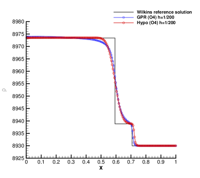
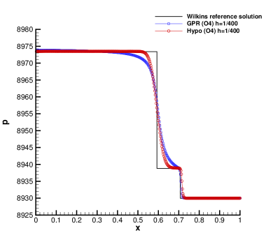
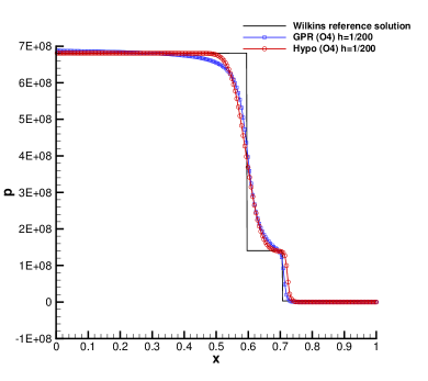
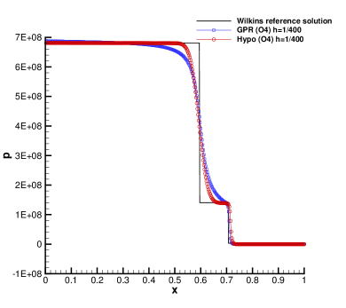
Figure 1: Comparison of the numerical solutions to the elastoplastic piston problem for the Wilkins and GPR model obtained with ALE ADER-WENO fourth order schemes. The density distribution (top row) and pressure distribution (bottom row) at final time $t_{\text{final}}=150\cdot 10^{-6}$ are shown along side with the exact solution (solid lines) of the Wilkins model. Each plot shows the numerical results computed with the GPR model (squares) and the Wilkins model (circles) for two different computational grids with characteristic mesh size of $h=1/200$ and $h=1/400$.

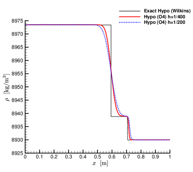
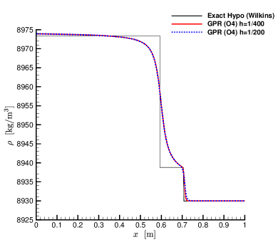
Figure 2: Comparison of the solution convergence rate for elastoplastic piston problem of the hypoelastic-type Wilkins model (left) and the hyperelastic-type GPR model (right). Because the plastic wave is continuous in the relaxation GPR model, the solutions to the GPR model obtained on a coarse and fine meshes with 4-th order method are almost indistinguishable in the plastic wave.

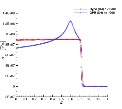
Figure 3: The intensity of tangential stresses $\sigma=\sqrt{3\text{tr}(\bm{\sigma}^{\prime 2})/2}$ for the elastic-plastic piston problem at final time $t_{\text{final}}=150\cdot 10^{-6}$ for Wilkins model and GPR model.

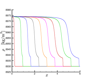
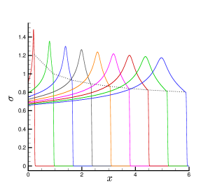
Figure 4: Long-time integration of the elastic-plastic piston problem for the GPR model. An unsteady evolution of the elastic precursor magnitude (dotted line on the right plot) is observed. The third order accurate scheme on a mesh with the characteristic size of $h=1/200$ was used.

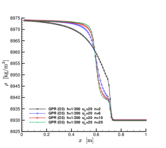
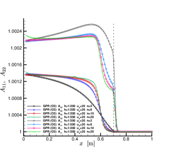
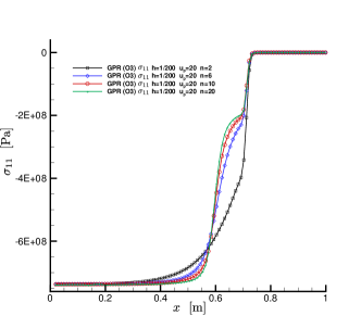
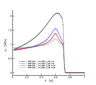
Figure 5: Elastic-plastic piston problem for the GPR model run with the same piston velocity $u_{p}=20$ for different values of the parameter $n$. The third order accurate scheme on a mesh with the characteristic size of $h=1/200$ was used.

6.2 Elastic vibrations of a Beryllium plate

This problem simulates the purely elastic vibrations of a beryllium plate loaded by an initial velocity distribution that is not zero [23, 19]. The computational domain is initially set to $\Omega(t=0)=[-3;3]\times[-0.5;0.5]$ and the mesh is made of $3210$ cells with a characteristic mesh size of $h=0.0065$. Free traction boundary conditions are considered everywhere. The plate is initialized with the reference density and pressure for beryllium taken from Table 2. The distortion field ${\bm{A}}$ of the hyperelastic model is initially set to identity while ${\bm{S}}=\bm{0}$ for the hypoelastic model. The velocity field is given by $\mathbf{v}=(0,v(x))$ where

$$v(x)=A\omega\left\{C_{1}\left(\sinh(\Omega(x+3))+\sin(\Omega(x+3))\right)-S_{1}\left(\cosh(\Omega(x+3))+\cos(\Omega(x+3))\right)\right\},$$ (60)

with $\Omega=0.7883401241$, $\omega=0.2359739922$, $A=0.004336850425$, $S_{1}=57.64552048$ and $C_{1}=56.53585154$. The final time is set to $t_{f}=53.25$ according to [23] such that it corresponds to two complete flexural periods $\omega$. In Figs. 6 and 7 we present the pressure and the vertical velocity component respectively for intermediate times $t=8^{-6}$, $t=15^{-6}$, $t=23^{-6}$ and $t=32^{-6}$ which cover approximately one flexural period. The color scales are identical to allow for a direct comparison of two models. Qualitatively the plate is behaving as expected and comparably for those two models. The oscillations decay only due to the numerical dissipation. Only tiny differences between the solutions can be observed meaning that we are rather in the linear elastic regime. Moreover, these third order accurate results visually compare well against known results from other Lagrangian schemes [152, 23].

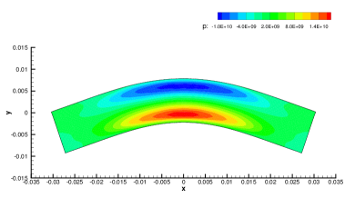
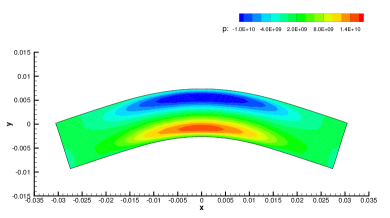
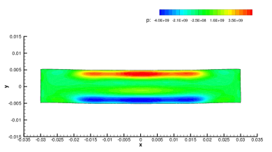
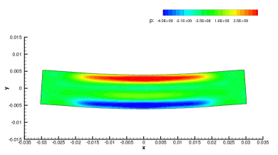
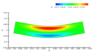
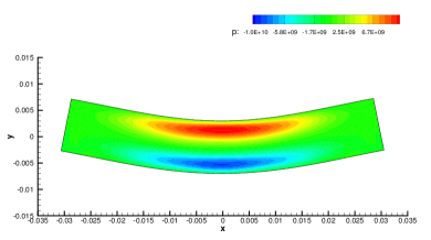
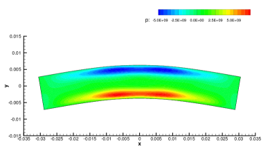
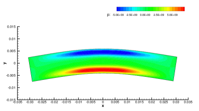
Figure 6: Pressure contours obtained with ALE ADER-WENO third order schemes for the oscillating Beryllium plate at output times $t=8\cdot 10^{-6}$, $t=16\cdot 10^{-6}$, $t=24\cdot 10^{-6}$ and $t=32\cdot 10^{-6}$ (from top row to bottom row). Left column: hypoelastic Wilkins model. Right column: hyperelastic GPR model.

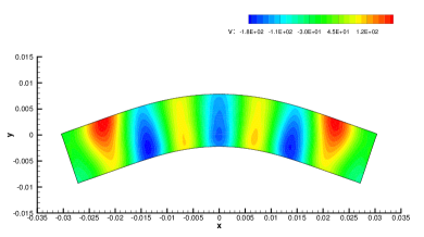
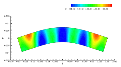
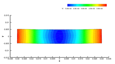
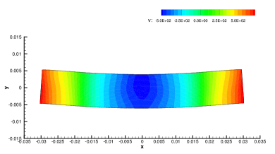
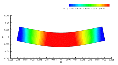
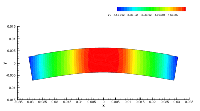
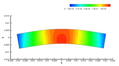
Figure 7: Velocity contours obtained with ALE ADER-WENO third order schemes for the oscillating Beryllium plate at output times $t=8\cdot 10^{-6}$, $t=16\cdot 10^{-6}$, $t=24\cdot 10^{-6}$ and $t=32\cdot 10^{-6}$ (from top row to bottom row). Left column: hypoelastic Wilkins model. Right column: hyperelastic GPR model.

6.3 Cylindrical shell compression

The next test case is known as the Verney problem [164, 92, 165] but we consider the problem statement as it is proposed by Howell and Ball in [83]. It consists in a cylindrical beryllium shell which collapses responding to an initial inwardly directed radial velocity field. The initial setup is taken from [92]. The shell $\Omega$ with inner radius $R_{i}=8\times 10^{-2}$m and outer radius $R_{o}=10\times 10^{-2}$m is made of beryllium under Mie-Gruneisen equation of state. In this test case, the material experiences elastoplastic deformations. Initial pressure is set to $p_{0}=10^{-6}$Pa and the radial velocity magnitude is given by $v_{0}(r)=-V_{0}\left(\frac{R_{i}}{r}\right)^{2}$, where we have chosen $V_{0}=417.10$m/s. The initial kinetic energy due to the velocity distribution is entirely dissipated by the plastic deformation of the material leading to a deceleration of the shell. At the end of the simulation, set to $t_{\text{final}}=125\mu$s, the shell arrives at a complete rest state for a value of the inner/outer radii equal to $r_{i}=5\times 10^{-2}$m and $r_{o}=7.81\times 10^{-2}$m. This exact solution has been derived by Howall and Ball in [83] under the ideal plasticity assumption. Only one quarter of the shell is considered in Cartesian geometry and its associated unstructured mesh has a characteristic mesh size of $h=10^{-3}$ or $h=2\times 10^{-3}$, leading to about $98500$ and $197000$ cells, respectively. Free traction boundary conditions are considered on the inner and outer radii, while symmetric boundary conditions are used for points on the axis $x=0$ and $y=0$. The results of the pressure contours (top) and the plasticity map (bottom) are displayed in Fig. 8 at the final instant of time for both models; GPR on left panels, Wilkins on the right ones. It can be observed that while qualitatively equivalent, these results differ in the field representation while maintaining a good radial symmetry.

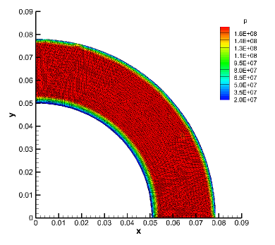
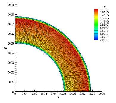
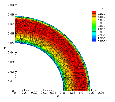
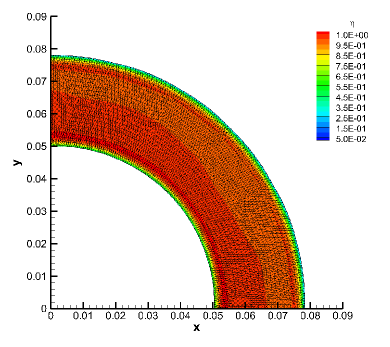
Figure 8: Pressure contours (top row) and plasticity map (bottom row) obtained with ALE ADER-WENO third order schemes for the shell compression test case with characteristic mesh size $h=10^{-3}$. Left column: hypoelastic Wilkins model. Right column: hyperelastic GPR model.

Next on the top panels of Fig. 9 we present the classical plots of energy balance where we can observe the transfer of kinetic energy into internal energy with conserved total energy. We observed that the hypo-elastic model of Wilkins presents a shift in chronometry when the mesh is refined, meaning that one has not reached the mesh convergence for this model. Contrarily the hyper-elastic GPR model does not present such shift. At last the bottom panels of the same figure illustrate the evolution of the mean inner/outer radii of the shell and their convergence towards their exact values (black lines) for both resolutions and models. A little bit faster convergence with respect to the mesh refinement can be observed for the GPR model. Overall, these third order accurate results visually compare well against known results from other Lagrangian schemes [152]. The distribution of the norm of the deviatoric stress $\sigma=\sqrt{3\text{tr}(\bm{\sigma}^{\prime 2})/2}$ is plotted in Fig. 9 versus radius. From these plots, one can judge about the degree of symmetry violation in our simulations. Thus, the distribution of $\sigma$ looks perfectly symmetric (all points lie on a single line) for the GPR model, while it is less symmetric for the Wilkins model.

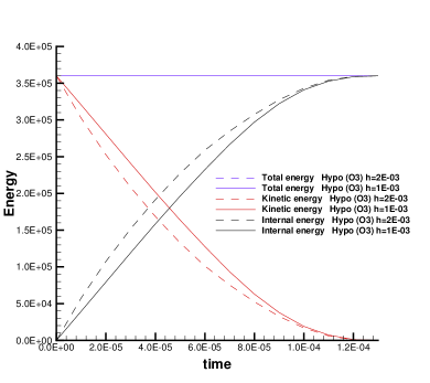
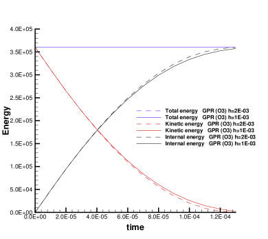
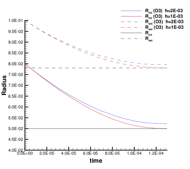
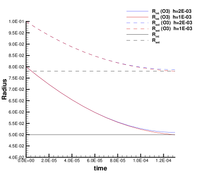
Figure 9: Top: analysis of energy conservation for the shell collapse test problem for both computational meshes and governing equations. Bottom: time evolution of the internal and external radius for both computational meshes and governing equations.

6.4 Taylor bar impact on a wall

This problem consists of the impact of a two-dimensional aluminum bar impacting on a rigid wall. Initially proposed as a cylindrical bar by Taylor [156], a planar geometry counterpart has been designed and simulated in [94, 105]. This later setup is considered in this paper. The computational domain is the initial projectile $\Omega(t=0)=[0:5]\times[0:1]$ and the mesh is made of about $8960$ ($h=0.10$) or $35872$ ($h=0.05$) cells. The final time is set to $t_{\text{final}}=0.005$. We consider aluminum material with the initial reference data from Table 2. Only the initial velocity is set to ${\bm{v}}=(-150,0)$. The boundary conditions are free traction for all boundaries except the left boundary which is a wall type. Although there exists no exact solution for this problem it is nonetheless employed for robustness and accuracy benchmarking. During the impact the kinetic energy is entirely converted into the internal energy through plastic dissipation. The results are displayed in Fig. 10 where we have plotted the meshes and the norm of the deviatoric stress $\sigma=\sqrt{3\text{tr}(\bm{\sigma}^{\prime 2})/2}$ in colors for a coarse (top) and refined mesh (bottom panel) for the hypoelastic model of Wilkins (left column) and the hyperelastic GPR model (right column). Since the same color scale is used, we can observe that the two models produce different distribution of $\sigma$ even if the general behavior of the rod is alike. In Fig. 11, we present the internal, kinetic and total energies for Wilkins model on the left and GPR model on the right for the coarse (dashed line) and fine (straight line) mesh results. As expected for both models, the total energy is conserved and the kinetic energy is decreasing to the benefit of the internal energy up to the time at which the bar stops moving. At this time the whole kinetic energy has been converted into the internal energy. On the middle panels of Fig. 11, we also plot the evolution of the length of the bar. It seems that for the hyperelastic GPR model the convergence towards its limit is mildly dependent on the mesh resolution unlike the hypoelastic model of Wilkins. Note that such mesh resolution dependency has already been observed in [105]. At last, the bottom panel of Fig. 11 presents the position comparison of the bar side boundary as a function of $x$. Five different times are plotted for both models. We can observe that the shape of the bar is truly different already at the third time corresponding to the middle of the simulation. The differences do increase in time leading to rather different final shapes.

Finally, we remark that the plasticity models which are based on the ideal plasticity constitutive law, like the Wilkins model, usually require an incorporation of an extra strain-hardening scalar parameter in order to fit experimental data. On the other hand, the strain hardening due to the finiteness of the rate of the dislocation nucleation is, in fact, accounting for in the rate dependent character of the GPR model and does not require the introducing of extra state variables, and a good agreement with the experimental data can be achieved [7, 81] with a proper model for the strain dissipation time $\tau$.

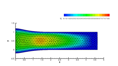
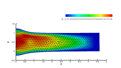
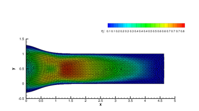
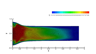
Figure 10: Plasticity color map of the Taylor rod test problem at the final time $t_{\text{final}}=0.005$ computed on an unstructured grid of characteristic mesh size $h=0.10$ (top row) and $h=0.05$ (middle row) with ADER-WENO third order schemes. Left column: hypoelastic Wilkins model results. Right column: hyperelastic GPR model results.

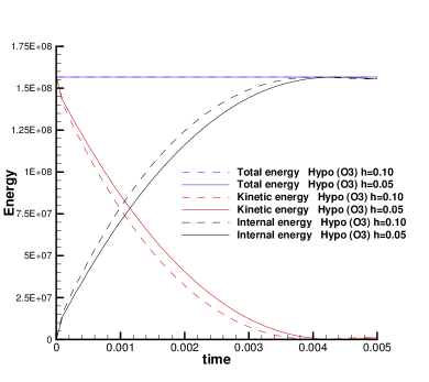
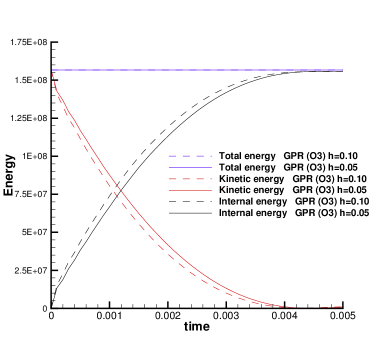
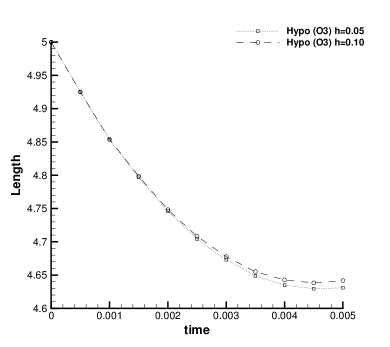
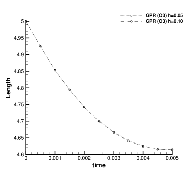
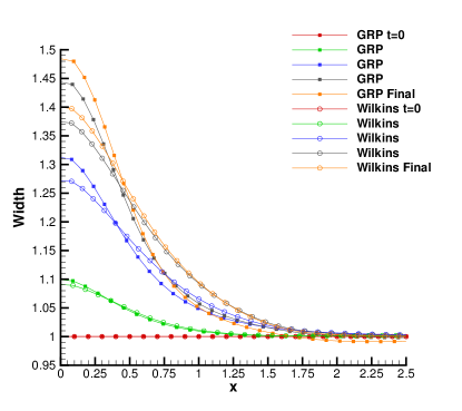
Figure 11: Top: analysis of energy conservation for the Taylor rod test problem for both computational meshes and governing equations. Middle: time evolution of the target length for both computational meshes and governing equations. Bottom: diagnostics on the bar width for $5$ time instants.

6.5 Elastic shear layer test

Here, we propose to solve a very simple test case which aims at showing the different responses of the hypoelastic and the hyperelastic materials in the non-linear elastic regime. The rectangular computational domain $\Omega(t=0)=[0:1]\times[0:0.1]$ is paved with $200\times 10$ square cells. The material is characterized by $\rho_{0}=1$, $c_{v}=c_{0}=c_{s}=1$ and the static yield strength $\sigma_{Y}=10^{20}$ is set to a very large value to avoid plastic deformations to occur. The stiffened gas equations of state is used with $\gamma=1.4$ and $\pi_{\infty}=0$. The initial conditions are given in terms of a classical one-dimensional Riemann problem where a discontinuity is located at $x_{d}=0.5$ and separates the right state $\mathbf{U}_{R}=(\rho_{R},u_{R},v_{R},p_{R})=(\rho_{0},0,v^{s},1)$ from the left one $\mathbf{U}_{L}=(\rho_{L},u_{L},v_{L},p_{L})=(\rho_{0},0,-v^{s},1)$. For the GPR model the distortion tensor is initialized with the identity matrix, i.e. ${\bm{A}}={\bm{I}}$, while the shear velocity is assigned two different values, namely $v^{s}_{1}=10^{-3}$ and $v^{s}_{2}=1$. The numerical results have been computed using a fourth order ADER Discontinuous Galerkin discretization (ADER-DG), supplemented with the finite volume subcell limiter presented in [46, 172, 18] and they are depicted in Fig. 12. When the shear stress is mild, then the linear elasticity equations are recovered from both models, and, as expected, the results are almost identical, see left panels. On the contrary, the hyperelastic model computes a totally different solution (in terms of location, amplitude and shape of the waves) when the material is subjected to strong shear. This is of course not surprising, because the Wilkins model was designed for the regimes when the elastic deformations are small, while its extension to large non-linear elastic deformations is rather problematic and requires retaining more terms in the general hypoelastic time evolution equation (11) and, what is more challenging, it requires solution dependent elastic moduli in (11), e.g. see [93]. This is why hypoelastic models are only very rarely used for modeling large elastic deformations (occurring for example in rubber). On the contrary, the hyperelastic models, and in particular the GPR model, provide a more flexible framework for modeling linear and non-linear elastic and elastoplastic deformations.

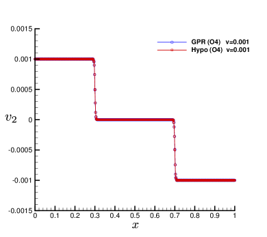
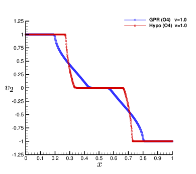
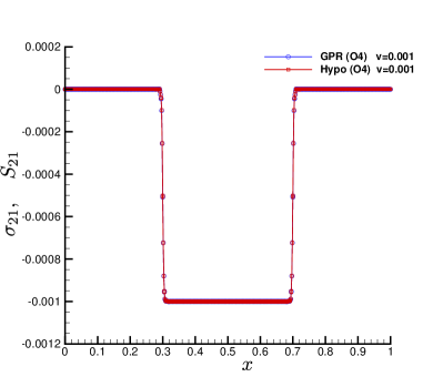
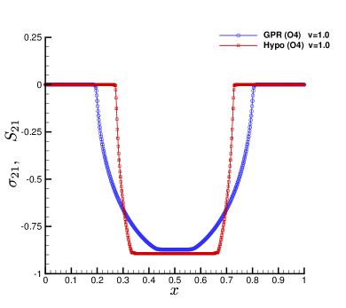
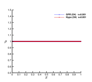
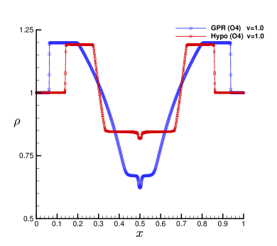
Figure 12: Shear layer test case results computed with ADER-DG fourth order scheme with initial shear velocity $v^{s}_{1}=10^{-3}$ (left column) or $v^{s}_{2}=1$ (right column) for both models are shown: velocity along the $y-$axis (top row), shear stresses $\sigma_{21}$ and $S_{21}$ (middle row) and density (bottom row).

6.6 Elastic rotor problem

Finally, both physical models are used to simulate the solid rotor problem proposed in [35] for the equations of nonlinear hyperelasticity. This test case consists of a homogeneous elastic material with a circular part subject to a sudden velocity impulse with the angular velocity $\omega$. It might be interpreted as a highly simplified model for the inner (rotating) and the outer (fixed) part of a bearing which are suddenly attached together via spontaneous welding by friction. The computational domain is the square $\Omega(t=0)=[-0.5:0.5]\times[-0.5:0.5]$ which is discretized with a Cartesian mesh of characteristic mesh size $h=0.02$. Transmissive boundary conditions are set everywhere and the final time is chosen to be $t_{\text{final}}=0.005$. The rotor radius is $R_{i}=0.1$ while $r=\sqrt{x^{2}+y^{2}}$ denotes the generic radial coordinate. We select two different angular frequencies, namely $\omega_{1}=10^{-2}$ and $\omega_{2}=10$, so that the tangential velocity of the rotor is $v_{t,1}=10^{-3}$ and $v_{t,2}=1$ at $r=R_{i}$, respectively. The material parameters are the same as the ones used for the shear layer test problem from the previous section. The simulations are performed using a fourth order ADER-DG scheme and the numerical results are shown in Figs. 13 and 14 for $v_{t,1}=10^{-3}$ and $v_{t,2}=1$ respectively. Shear waves traveling into both the rotor and the stator as well as pressure waves can be observed. Even in this case, if the shear stresses are not too strong like in Fig. 13 with $v_{t,1}=10^{-3}$, the hypoelastic Wilkins model and the hyperelastic GPR model show almost the same behavior. This is expected because, in this case, they both reduce to the equations of linear elasticity. However, when the deformations are larger, see Fig. 14 with $v_{t,2}=1$, the solutions of the models are different which, as in the previous example, can be explained by the inability of Wilkins model to deal with large reversible non-linear elastic deformations, and its extension to finite strains is a rather complicated process.

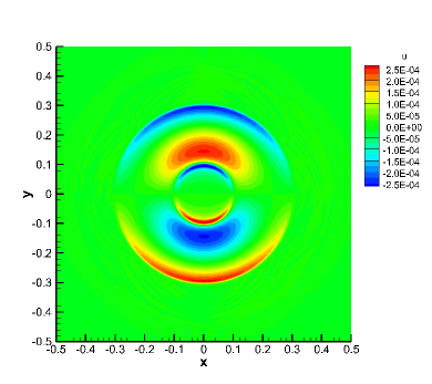
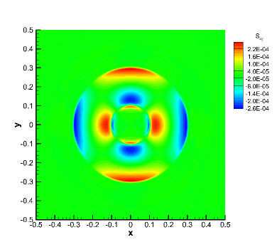
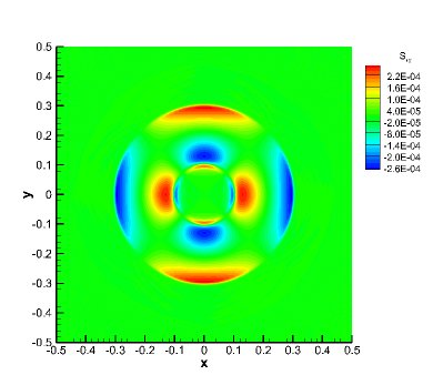
Figure 13: Results for the solid rotor problem obtained with ADER-DG fourth order scheme with initial angular velocity of the rotor of ${\bm{v}}\times\omega=0.001$. Horizontal velocity (top row) and stress tensor component $\sigma_{21}$ and $S_{21}$ (bottom row) are displayed. The Wilkins model results are displayed on the left panels, GPR model ones on the right panels.

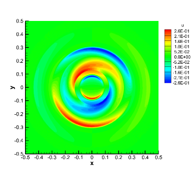
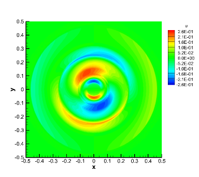
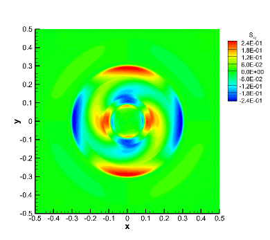
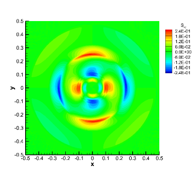
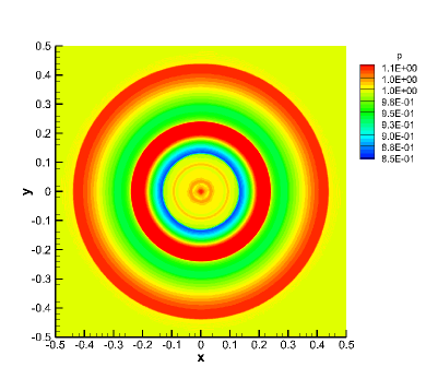
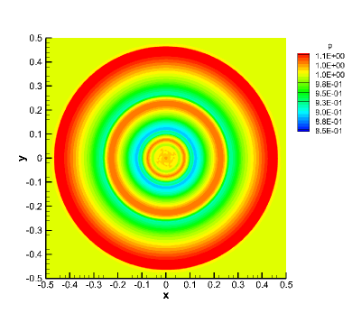
Figure 14: Results for the solid rotor problem obtained with ADER-DG fourth order scheme with initial angular velocity of the rotor of ${\bm{v}}\times\omega=1.0$. Horizontal velocity (top row), stress tensor component $\sigma_{21}$ and $S_{21}$ (middle row) and pressure $p$ (bottom row) are displayed. The Wilkins model results are displayed on the left panels, GPR model ones on the right panels.

7 Conclusion and Perspectives

The goal of this paper was to compare the GPR hyperelastic model against the well-known hypoelastic model of Wilkins. While the former model is derived in the framework of symmetric hyperbolic and thermodynamically compatible equations and somewhat more complex, the latter is apparently simpler but thermodynamically inconsistent and suffers from modeling 'choices' that are sometimes difficult to justify. We have implemented both models into the same simulation codes based either on a high order direct ALE framework on moving unstructured meshes, or a high order ADER-Discontinuous Galerkin scheme with subcell finite volume limiter on fixed Cartesian grids. We have elaborated the differences between the two models from the modeling point of view. Moreover, we have performed a systematic comparison of their numerical behavior on a set of well known test cases.

A large set of benchmark problems in 1D and 2D have been simulated. In this work the materials have been described by a Mie-Grüneisen or stiffened gas equation of state for the hydrodynamic pressure. In the GPR model, a simple equation of state based on the invariants of the trace-free part of the metric tensor $\mathbf{G}={\bm{A}}^{T}{\bm{A}}$ has been used. The numerical results of both models have been reported to assess their differences, and, also, to show some circumstances where the models behave alike. We have observed that on the most simple elastic tests, both models produce very much resembling results. More differences are observed when transient plastic deformations occur since the inelasticity is incorporated in a fundamentally different way in these two models, in a rate-dependent manner in the GPR model and in the rate-independent ideal plasticity manner in the Wilkins model. This fact was already expected from the analysis of the models. Since the numerical framework used for the comparison is the same, we can therefore clearly attribute those difference to the intrinsically different properties of the models.

Even more differences have been observed in the case when the material undergoes finite elastic deformations. In this case, as it was expected, the hypoelastic Wilkins model has to be modified by adding extra differential terms to the evolution equation of the stress deviator with solution dependent elastic modulus, which is not a trivial task. On the contrary, due to the hyperelastic character of the GPR model, no new differential terms should be applied to the model, but only the equation of state should be adjusted, which is more convenient from the practical viewpoint than modifying the evolution equation for the stress deviator.

We would like to mention that although Wilkins model is thermodynamically inconsistent, this model is extremely simple, in particular when considering complex boundary conditions in multi-dimensions. Contrarily the GPR model, appealing from the modeling point of view, is more complex to implement and demands extra care when boundary conditions are involved. This will be the subject of a forthcoming work.

In the future, we plan to investigate the hyperelastic GPR model for different equations of state and to apply it also to non-Newtonian fluids, in order to widen its range of practical applicability. Moreover, we plan to compare the numerical results against available laboratory experiments. Other directions of research will be dedicated to enriching the model capabilities by the ability to deal with complex physics of inelastic deformations in order to account for damaging and dislocation dynamics via an explicit inclusion of the evolution equation of the damage order parameter [135, 141] and of the Burgers tensor [125], respectively.

References

- Andreotti et al. [2013] Andreotti, B., Forterre, Y., Pouliquen, O., 2013. Granular Media: Between Fluid and Solid. Cambridge University Press. URL: http://www.edition-sciences.com/milieux-granulaires-entre-fluide-et-solide.htm, doi:10.1080/00107514.2014.885579.
- Balmforth et al. [2014] Balmforth, N.J., Frigaard, I.A., Ovarlez, G., 2014. Yielding to Stress : Recent Developments in Viscoplastic Fluid Mechanics. Annual Review of Fluid Mechanics 46, 121–146. doi:10.1146/annurev-fluid-010313-141424.
- Balsara et al. [2007] Balsara, D., Altmann, C., Munz, C.D., Dumbser, M., 2007. A sub-cell based indicator for troubled zones in {RKDG} schemes and a novel class of hybrid {RKDG}+{HWENO} schemes. Journal of Computational Physics 226, 586–620.
- Balsara and Shu [2000] Balsara, D., Shu, C., 2000. Monotonicity perserving weighted essentially non-oscillatory schemes with increasingly high order of accuracy. J. Comput. Phys. 160, 405–452.
- Barton et al. [2013] Barton, P., Deiterding, R., Meiron, D., Pullin, D., 2013. Eulerian adaptive finite-difference method for high-velocity impact and penetration problems. Journal of Computational Physics 240, 76–99. URL: https://www.sciencedirect.com/science/article/pii/S0021999113000442?via{%}3Dihub, doi:10.1016/J.JCP.2013.01.013.
- Barton et al. [2009a] Barton, P., Drikakis, D., Romenski, E., Titarev, V., 2009a. Exact and approximate solutions of Riemann problems in non-linear elasticity. Journal of Computational Physics 228, 7046–7068. URL: http://linkinghub.elsevier.com/retrieve/pii/S0021999109003386, doi:10.1016/j.jcp.2009.06.014.
- Barton and Romenski [2012] Barton, P., Romenski, E., 2012. On Computational Modelling Of Strain-Hardening Material Dynamics. Communications in Computational Physics 11, 1525–1546. URL: http://www.journals.cambridge.org/abstract{_}S1815240600002814, doi:10.4208/cicp.171210.270511a.
- Barton [2018] Barton, P.T., 2018. A level-set based Eulerian method for simulating problems involving high strain-rate fracture and fragmentation. International Journal of Impact Engineering 117, 75–84. URL: https://doi.org/10.1016/j.ijimpeng.2018.03.002, doi:10.1016/j.ijimpeng.2018.03.002.
- Barton et al. [2009b] Barton, P.T., Drikakis, D., Romenski, E.I., 2009b. An Eulerian finite-volume scheme for large elastoplastic deformations in solids. International Journal for Numerical Methods in Engineering 81, n/a–n/a. URL: http://doi.wiley.com/10.1002/nme.2695, doi:10.1002/nme.2695.
- Benzoni-Gavage and Serre [2007] Benzoni-Gavage, S., Serre, D., 2007. Multidimensional Hyperbolic Partial Differential Equations. Oxford University Press, Oxford.
- Beris and Edwards [1994] Beris, A.N., Edwards, B.J., 1994. Thermodynamics of Flowing Systems: With Internal Microstructure. Oxford University Press, USA.
- Besseling [1968] Besseling, J.F., 1968. A thermodynamic approach to rheology, in: Parkus, H., Sedov, L.I. (Eds.), Irreversible Aspects of Continuum Mechanics and Transfer of Physical Characteristics in Moving Fluids, Springer Vienna. pp. 16–53. doi:10.1007/978-3-7091-5581-3_2.
- Besseling and Van Der Giessen [1994] Besseling, J.F., Van Der Giessen, E., 1994. Mathematical Modelling of Inelastic Deformation. Springer US, Boston, MA. URL: http://link.springer.com/10.1007/978-1-4899-7186-9, doi:10.1007/978-1-4899-7186-9.
- Boscheri [2016] Boscheri, W., 2016. High Order Direct Arbitrary-Lagrangian–Eulerian (ALE) Finite Volume Schemes for Hyperbolic Systems on Unstructured Meshes. Archives of Computational Methods in Engineering , 1–51doi:10.1007/s11831-016-9188-x.
- Boscheri and Dumbser [2013] Boscheri, W., Dumbser, M., 2013. Arbitrary–Lagrangian–Eulerian One–Step WENO Finite Volume Schemes on Unstructured Triangular Meshes. Communications in Computational Physics 14, 1174–1206.
- Boscheri and Dumbser [2014] Boscheri, W., Dumbser, M., 2014. A Direct Arbitrary-Lagrangian-Eulerian ADER-WENO Finite Volume Scheme on Unstructured Tetrahedral Meshes for Conservative and Nonconservative Hyperbolic Systems in 3D. Journal of Computational Physics 275, 484–523.
- Boscheri and Dumbser [2016] Boscheri, W., Dumbser, M., 2016. An Efficient Quadrature-Free Formulation for High Order Arbitrary-Lagrangian-Eulerian ADER-WENO Finite Volume Schemes on Unstructured Meshes. Journal of Scientific Computing 66, 240–274.
- Boscheri and Dumbser [2017] Boscheri, W., Dumbser, M., 2017. Arbitrary-Lagrangian–Eulerian Discontinuous Galerkin schemes with a posteriori subcell finite volume limiting on moving unstructured meshes. Journal of Computational Physics 346, 449–479.
- Boscheri et al. [2016] Boscheri, W., Dumbser, M., Loubere, R., 2016. Cell centered direct Arbitrary-Lagrangian-Eulerian ADER-WENO finite volume schemes for nonlinear hyperelasticity. Computers and Fluids 134–135, 111–129. doi:10.1016/j.compfluid.2016.05.004.
- Boscheri and Loubère [2016] Boscheri, W., Loubère, R., 2016. High order accurate direct Arbitrary-Lagrangian-Eulerian ADER-MOOD finite volume schemes for non-conservative hyperbolic systems with stiff source terms. Communications in Computational Physics 21, 271–312.
- Boscheri et al. [2015] Boscheri, W., Loubère, R., Dumbser, M., 2015. Direct arbitrary-lagrangian-eulerian ader-mood finite volume schemes for multidimensional hyperbolic conservation laws. J. Comput. Physics , 56–87.
- Burton et al. [2013] Burton, D., Carney, T., Morgan, N., Sambasivan, S., Shashkov, M., 2013. A cell-centered lagrangian godunov-like method for solid dynamics. Computers and Fluids 83, 33 – 47. URL: http://www.sciencedirect.com/science/article/pii/S0045793012003647, doi:http://dx.doi.org/10.1016/j.compfluid.2012.09.008. numerical methods for highly compressible multi-material flow problems.
- Burton et al. [2015] Burton, D., Morgan, N., Carney, T., Kenamond, M., 2015. Reduction of dissipation in lagrange cell-centered hydrodynamics (cch) through corner gradient reconstruction (cgr). Journal of Computational Physics 299, 229–280.
- Castro et al. [2008] Castro, M.J., Gallardo, J.M., López, J.A., Parés, C., 2008. Well-balanced high order extensions of Godunov's method for semilinear balance laws. SIAM Journal of Numerical Analysis 46, 1012–1039.
- Castro et al. [2006] Castro, M.J., Gallardo, J.M., Parés, C., 2006. High-order finite volume schemes based on reconstruction of states for solving hyperbolic systems with nonconservative products. Applications to shallow-water systems. Mathematics of Computation 75, 1103–1134.
- Ciarlet [1988] Ciarlet, P.G., 1988. Mathematical Elasticity: Three-dimensional elasticity, Volume 1. volume 20. Elsevier.
- Clain et al. [2011] Clain, S., Diot, S., Loubère, R., 2011. A high-order finite volume method for systems of conservation laws—Multi-dimensional Optimal Order Detection ({MOOD}). Journal of Computational Physics 230, 4028–4050. URL: http://www.sciencedirect.com/science/article/pii/S002199911100115X, doi:10.1016/j.jcp.2011.02.026.
- Clayton and Lloyd [2018] Clayton, J.D., Lloyd, J.T., 2018. Analysis of nonlinear elastic aspects of precursor attenuation in shock-compressed metallic crystals. Journal of Physics Communications 2, 045032. URL: https://doi.org/10.1088/2399-6528/aabc43http://stacks.iop.org/2399-6528/2/i=4/a=045032?key=crossref.55f58d2caa2d9b859535fd4539283b1d, doi:10.1088/2399-6528/aabc43.
- Cockburn et al. [1990] Cockburn, B., Hou, S., Shu, C.W., 1990. The Runge-Kutta local projection discontinuous Galerkin finite element method for conservation laws IV: the multidimensional case. Mathematics of Computation 54, 545–581.
- Cockburn and Shu [1998] Cockburn, B., Shu, C.W., 1998. The {Runge}-{Kutta} discontinuous {Galerkin} method for conservation laws {V}: multidimensional systems. Journal of Computational Physics 141, 199–224.
- Dafermos [2005] Dafermos, C.M., 2005. Hyperbolic conservation laws in continuum physics. Springer-Verlag, Berlin.
- Diot et al. [2012] Diot, S., Clain, S., Loubère, R., 2012. Improved detection criteria for the Multi-dimensional Optimal Order Detection ({MOOD}) on unstructured meshes with very high-order polynomials. Computers and Fluids 64, 43–63. URL: http://www.sciencedirect.com/science/article/pii/S0045793012001909, doi:10.1016/j.compfluid.2012.05.004.
- Diot et al. [2013] Diot, S., Loubère, R., Clain, S., 2013. The {MOOD} method in the three-dimensional case: Very-High-Order Finite Volume Method for Hyperbolic Systems. International Journal of Numerical Methods in Fluids 73, 362–392.
- Dumbser [2010] Dumbser, M., 2010. Arbitrary High Order {PNPM} Schemes on Unstructured Meshes for the Compressible {Navier–Stokes} Equations. Computers & Fluids 39, 60–76.
- Dumbser et al. [2008a] Dumbser, M., Balsara, D., Toro, E.F., Munz, C.D., 2008a. A Unified Framework for the Construction of One-Step Finite-Volume and discontinuous {Galerkin} schemes. Journal of Computational Physics 227, 8209–8253.
- Dumbser and Boscheri [2013] Dumbser, M., Boscheri, W., 2013. High-order unstructured Lagrangian one–step WENO finite volume schemes for non–conservative hyperbolic systems: Applications to compressible multi–phase flows. Computers and Fluids 86, 405–432.
- Dumbser et al. [2017a] Dumbser, M., Boscheri, W., Semplice, M., Russo, G., 2017a. Central weighted ENO schemes for hyperbolic conservation laws on fixed and moving unstructured meshes. SIAM Journal on Scientific Computing 39, A2564–A2591.
- Dumbser et al. [2009a] Dumbser, M., Castro, M., Parés, C., Toro, E.F., 2009a. {ADER} Schemes on Unstructured Meshes for Non-Conservative Hyperbolic Systems: Applications to Geophysical Flows. Computers and Fluids 38, 1731—-1748.
- Dumbser et al. [2009b] Dumbser, M., Castro Díaz, M.J., Parés, C., Toro, E.F., 2009b. {ADER} schemes on unstructured meshes for nonconservative hyperbolicsystems: {A}pplications to geophysical flows. Computers {&} Fluids 38, 1731–1748. URL: http://www.sciencedirect.com/science/article/pii/S0045793009000498.
- Dumbser et al. [2008b] Dumbser, M., Enaux, C., Toro, E.F., 2008b. Finite Volume Schemes of Very High Order of Accuracy for Stiff Hyperbolic Balance Laws. Journal of Computational Physics 227, 3971–4001.
- Dumbser et al. [2007] Dumbser, M., Käser, M., Titarev, V.A., Toro, E.F., 2007. Quadrature-Free Non-Oscillatory Finite Volume Schemes on Unstructured Meshes for Nonlinear Hyperbolic Systems. Journal of Computational Physics 226, 204–243.
- Dumbser and Loubère [2016] Dumbser, M., Loubère, R., 2016. A simple robust and accurate a posteriori sub-cell finite volume limiter for the discontinuous Galerkin method on unstructured meshes. Journal of Computational Physics 319, 163–199.
- Dumbser et al. [2016] Dumbser, M., Peshkov, I., Romenski, E., Zanotti, O., 2016. High order ADER schemes for a unified first order hyperbolic formulation of continuum mechanics: viscous heat-conducting fluids and elastic solids. Journal of Computational Physics 314, 824–862. URL: https://linkinghub.elsevier.com/retrieve/pii/S0021999116000693http://arxiv.org/abs/1511.08995http://dx.doi.org/10.1016/j.jcp.2016.02.015, doi:10.1016/j.jcp.2016.02.015, arXiv:1511.08995.
- Dumbser et al. [2017b] Dumbser, M., Peshkov, I., Romenski, E., Zanotti, O., 2017b. High order ADER schemes for a unified first order hyperbolic formulation of Newtonian continuum mechanics coupled with electro-dynamics. Journal of Computational Physics 348, 298--342. URL: http://dx.doi.org/10.1016/j.jcp.2017.07.020https://www.sciencedirect.com/science/article/pii/S0021999117305284, doi:10.1016/j.jcp.2017.07.020, arXiv:1612.02093.
- Dumbser et al. [2014a] Dumbser, M., Zanotti, O., Loubère, R., Diot, S., 2014a. A posteriori subcell limiting of the discontinuous Galerkin finite element method for hyperbolic conservation laws. Journal of Computational Physics 278, 47--75.
- Dumbser et al. [2014b] Dumbser, M., Zanotti, O., Loubère, R., Diot, S., 2014b. A posteriori subcell limiting of the discontinuous galerkin finite element method for hyperbolic conservation laws. Journal of Computational Physics 278, 47--75.
- Dunatunga and Kamrin [2015] Dunatunga, S., Kamrin, K., 2015. Continuum modelling and simulation of granular flows through their many phases. Journal of Fluid Mechanics 779, 483--513. URL: http://www.journals.cambridge.org/abstract{_}S0022112015003833, doi:10.1017/jfm.2015.383.
- Dupret and Marchal [1986] Dupret, F., Marchal, J., 1986. Loss of evolution in the flow of viscoelastic fluids. Journal of Non-Newtonian Fluid Mechanics 20, 143--171.
- E. I. Romenskii [1984] E. I. Romenskii, 1984. Conservation laws and symmetric form of equations of the nonlinear theory of elasticity. Boundary Value Problems for Partial Differential Equations 1, 132--143.
- Eckart [1948] Eckart, C., 1948. The Thermodynamics of Irreversible Processes. IV. The Theory of Elasticity and Anelasticity. Physical Review 73, 373--382. URL: https://link.aps.org/doi/10.1103/PhysRev.73.373, doi:10.1103/PhysRev.73.373.
- Favrie and Gavrilyuk [2015] Favrie, N., Gavrilyuk, S., 2015. A wellposed hypoelastic model derived from a hyperelastic one. <Hal-01164353> URL: https://hal.archives-ouvertes.fr/hal-01164353.
- Favrie and Gavrilyuk [2012] Favrie, N., Gavrilyuk, S.L., 2012. Diffuse interface model for compressible fluid-Compressible elastic-plastic solid interaction. Journal of Computational Physics 231, 2695--2723.
- Frenkel [1955] Frenkel, J., 1955. Kinetic theory of liquids. Dover.
- Fridrich et al. [2017] Fridrich, D., Liska, R., Wendroff, B., 2017. Cell-centered Lagrangian Lax–Wendroff HLL hybrid method for elasto-plastic flows. Computers & Fluids 157, 164--174. URL: https://www.sciencedirect.com/science/article/pii/S0045793017303080, doi:10.1016/J.COMPFLUID.2017.08.030.
- Gallardo et al. [2007] Gallardo, J.M., Parés, C., Castro, M.J., 2007. On a well-balanced high-order finite volume scheme for shallow water equations with topography and dry areas. Journal of Computational Physics 227, 574--601.
- Gassner et al. [2011] Gassner, G., Dumbser, M., Hindenlang, F., Munz, C.D., 2011. Explicit One--Step Time Discretizations for Discontinuous {Galerkin} and Finite Volume Schemes Based on Local Predictors. Journal of Computational Physics 230, 4232--4247.
- Gavrilyuk et al. [2008a] Gavrilyuk, S., Favrie, N., Saurel, R., 2008a. Modelling wave dynamics of compressible elastic materials. Journal of Computational Physics 227, 2941--2969. doi:10.1016/j.jcp.2007.11.030.
- Gavrilyuk et al. [2008b] Gavrilyuk, S.L., Favrie, N., Saurel, R., 2008b. Modelling wave dynamics of compressible elastic materials. Journal of Computational Physics 227, 2941--2969.
- Godunov et al. [1970] Godunov, S., Deribas, A., Zabrodin, A., Kozin, N., 1970. Hydrodynamic effects in colliding solids. Journal of Computational Physics 5, 517--539. doi:10.1016/0021-9991(70)90078-1.
- Godunov et al. [1996] Godunov, S., Mikhailova, T., Romenskii, E., 1996. Systems of thermodynamically coordinated laws of conservation invariant under rotations. Siberian Mathematical Journal 37, 690--705.
- Godunov and Peshkov [2010] Godunov, S., Peshkov, I., 2010. Thermodynamically Consistent Nonlinear Model of Elastoplastic Maxwell Medium. Computational Mathematics and Mathematical Physics 50, 1409--1426. URL: https://link.springer.com/article/10.1134{%}2FS0965542510080117, doi:10.1134/S0965542510080117.
- Godunov and Romensky [1995] Godunov, S., Romensky, E., 1995. Thermodynamics, conservation laws and symmetric forms of differential equations in mechanics of continuous media, in: Computational Fluid Dynamics Review 1995. John Wiley, NY. volume 95, pp. 19--31. doi:10.1142/7799.
- Godunov [1961] Godunov, S.K., 1961. An interesting class of quasilinear systems. Dokl. Akad. Nauk SSSR 139(3), 521--523.
- Godunov [1972] Godunov, S.K., 1972. Symmetric form of the magnetohydrodynamic equation. Numerical Methods for Mechanics of Continuum Medium 3, 26--34. URL: https://pdfs.semanticscholar.org/5066/233d430f114fdf1d4c9c1ef5a67b365ac19f.pdf.
- Godunov [1978] Godunov, S.K., 1978. Elements of mechanics of continuous media. 1st russia ed., Nauka.
- Godunov et al. [1976a] Godunov, S.K., Demchuk, A.F., Kozin, N.S., Mali, V.I., 1976a. Interpolation formulas for maxwell viscosity of certain metals as a function of shear-strain intensity and temperature. Journal of Applied Mechanics and Technical Physics 15, 526--529. URL: http://link.springer.com/10.1007/BF00864733, doi:10.1007/BF00864733.
- Godunov et al. [1976b] Godunov, S.K., Denisenko, V.V., Kozin, N.S., Kuz'mina, N.K., 1976b. Use of relaxation viscoelastic model in calculating uniaxial homogeneous strains and refining the interpolation equations for maxwellian viscosity. Journal of Applied Mechanics and Technical Physics 16, 811--814. URL: http://link.springer.com/10.1007/BF00854096, doi:10.1007/BF00854096.
- Godunov et al. [1976c] Godunov, S.K., Denisenko, V.V., Kozin, N.S., Kuz'mina, N.K., 1976c. Use of relaxation viscoelastic model in calculating uniaxial homogeneous strains and refining the interpolation equations for maxwellian viscosity. Journal of Applied Mechanics and Technical Physics 16, 811--814. URL: http://link.springer.com/10.1007/BF00854096, doi:10.1007/BF00854096.
- Godunov and Kozin [1976] Godunov, S.K., Kozin, N.S., 1976. Shock structure in a viscoelastic medium with a nonlinear dependence of the Maxwellian viscosity on the parameters of the material. Journal of Applied Mechanics and Technical Physics 15, 666--671. URL: http://link.springer.com/10.1007/BF00851527, doi:10.1007/BF00851527.
- Godunov and Romenskii [1972] Godunov, S.K., Romenskii, E.I., 1972. Nonstationary equations of nonlinear elasticity theory in eulerian coordinates. Journal of Applied Mechanics and Technical Physics 13, 868--884. URL: http://link.springer.com/10.1007/BF01200547, doi:10.1007/BF01200547.
- Godunov and Romenskii [2003] Godunov, S.K., Romenskii, E.I., 2003. Elements of continuum mechanics and conservation laws. Kluwer Academic/Plenum Publishers.
- Godunov and Romensky [1996] Godunov, S.K., Romensky, E.I., 1996. Symmetric forms of thermodynamically compatible systems of conservation laws in continuum mechanics, in: ECCOMAS Conference on numerical methods in engineering, pp. 54--57.
- Gorsse et al. [2014] Gorsse, Y., Iollo, A., Milcent, T., Telib, H., 2014. A simple Cartesian scheme for compressible multimaterials. Journal of Computational Physics 272, 772--798. URL: https://www.sciencedirect.com/science/article/pii/S0021999114003374, doi:10.1016/J.JCP.2014.04.057.
- Green [1956] Green, A., 1956. Hypo-Elasticity and Plasticity. Proceedings of the Royal Society A: Mathematical, Physical Science 234, 46--59.
- Greenman et al. [1967] Greenman, W.F., Vreeland, T., Wood, D.S., 1967. Dislocation Mobility in Copper. Journal of Applied Physics 38, 3595--3603. URL: https://doi.org/10.1063/1.1702940http://aip.scitation.org/toc/jap/36/10http://aip.scitation.org/doi/10.1063/1.1710178, doi:10.1063/1.1710178.
- Grmela and Öttinger [1997] Grmela, M., Öttinger, H.C., 1997. Dynamics and thermodynamics of complex fluids. I. Development of a general formalism. Physical Review E 56, 6620--6632. doi:10.1103/PhysRevE.56.6620.
- Guinan and Steinberg [1974] Guinan, M., Steinberg, D., 1974. Pressure and temperature derivatives of the isotropic polycrystalline shear modulus for 65 elements. Journal of Physics and Chemistry of Solids 35, 1501--1512. URL: http://linkinghub.elsevier.com/retrieve/pii/S0022369774802787, doi:10.1016/S0022-3697(74)80278-7.
- Gurrutxaga-Lerma et al. [2015] Gurrutxaga-Lerma, B., Balint, D.S., Dini, D., Eakins, D.E., Sutton, A.P., 2015. Attenuation of the Dynamic Yield Point of Shocked Aluminum Using Elastodynamic Simulations of Dislocation Dynamics. Physical Review Letters 114, 174301. URL: https://link.aps.org/doi/10.1103/PhysRevLett.114.174301, doi:10.1103/PhysRevLett.114.174301.
- Gurtin et al. [2009] Gurtin, M., Fried, E., Anand, L., 2009. The mechanics and thermodynamics of continua. Cambridge University Press.
- Haider et al. [2017] Haider, J., Lee, C.H., Gil, A.J., Bonet, J., 2017. A first-order hyperbolic framework for large strain computational solid dynamics: An upwind cell centred Total Lagrangian scheme. International Journal for Numerical Methods in Engineering 109, 407--456. doi:10.1002/nme.5293.
- Hank et al. [2017] Hank, S., Gavrilyuk, S., Favrie, N., Massoni, J., 2017. Impact simulation by an Eulerian model for interaction of multiple elastic-plastic solids and fluids. International Journal of Impact Engineering 109, 104--111. URL: http://dx.doi.org/10.1016/j.ijimpeng.2017.06.003http://linkinghub.elsevier.com/retrieve/pii/S0734743X16303414, doi:10.1016/j.ijimpeng.2017.06.003.
- Hidalgo and Dumbser [2011] Hidalgo, A., Dumbser, M., 2011. {ADER} Schemes for Nonlinear Systems of Stiff Advection-Diffusion-Reaction Equations. Journal of Scientific Computing 48, 173--189.
- Howell and Ball [2002] Howell, B., Ball, G., 2002. A Free-Lagrange Augmented Godunov Method for the Simulation of Elastic–Plastic Solids. Journal of Computational Physics 175, 128--167. URL: https://www.sciencedirect.com/science/article/pii/S0021999101969311, doi:10.1006/JCPH.2001.6931.
- H.Zhu and J.Qiu [2013] H.Zhu, J.Qiu, 2013. An h-adaptive RKDG method with troubled-cell indicator for two-dimensional hyperbolic conservation laws. Advances in Computational Mathematics 39, 445--463. URL: http://dx.doi.org/10.1007/s10444-012-9287-7, doi:10.1007/s10444-012-9287-7.
- Israel [1976] Israel, W., 1976. Nonstationary irreversible thermodynamics: A causal relativistic theory. Annals of Physics 100, 310--331. URL: https://www.sciencedirect.com/science/article/pii/0003491676900646, doi:10.1016/0003-4916(76)90064-6.
- Jiang and Shu [1996] Jiang, G.S., Shu, C.W., 1996. Efficient Implementation of Weighted {ENO} Schemes. Journal of Computational Physics 126, 202--228.
- Johnson et al. [1970] Johnson, J.N., Jones, O.E., Michaels, T.E., 1970. Dislocation Dynamics and Single‐Crystal Constitutive Relations: Shock‐Wave Propagation and Precursor Decay. Journal of Applied Physics 41, 2330--2339. URL: http://aip.scitation.org/doi/10.1063/1.1659227, doi:10.1063/1.1659227.
- Johnston and Gilman [1959] Johnston, W.G., Gilman, J.J., 1959. Dislocation Velocities, Dislocation Densities, and Plastic Flow in Lithium Fluoride Crystals. Journal of Applied Physics 30. doi:10.1063/1.1735121.
- Joseph and Saut [1986] Joseph, D., Saut, J., 1986. Change of type and loss of evolution in the flow of viscoelastic fluids. Journal of Non-Newtonian Fluid Mechanics 20, 117--141. URL: https://www.sciencedirect.com/science/article/pii/0377025786800180http://linkinghub.elsevier.com/retrieve/pii/0377025786800180, doi:10.1016/0377-0257(86)80018-0.
- Jou et al. [2010] Jou, D., Casas-Vázquez, J., Lebon, G., 2010. Extended irreversible thermodynamics. Springer Berlin Heidelberg, Dordrecht. URL: http://link.springer.com/10.1007/978-90-481-3074-0, doi:10.1007/978-90-481-3074-0.
- J.Qiu and C-W.Shu [2005] J.Qiu, C-W.Shu, 2005. A Comparison of Troubled-Cell Indicators for {Runge--Kutta} Discontinuous {Galerkin} Methods Using Weighted Essentially Nonoscillatory Limiters. SIAM J. Sci. Comput. 27, 995--1013. URL: http://dx.doi.org/10.1137/04061372X, doi:10.1137/04061372X.
- Kamm et al. [2008] Kamm, J., Brock, J., Brandon, S., Cotrell, D., Johnson, B., Knupp, P., Trucano, T., Rider, W., Weirs, V., 2008. Enhanced verification test suite for physics simulations codes. Technical Report LA-14379 .
- Kim [2016] Kim, H.G., 2016. A comparative study of hyperelastic and hypoelastic material models with constant elastic moduli for large deformation problems. Acta Mechanica 227, 1351--1362. doi:10.1007/s00707-015-1554-5.
- Kluth and Després [2010] Kluth, G., Després, B., 2010. Discretization of hyperelasticity on unstructured mesh with a cell-centered lagrangian scheme. Journal of Computational Physics 229, 9092 -- 9118. URL: http://www.sciencedirect.com/science/article/pii/S0021999110004717, doi:http://dx.doi.org/10.1016/j.jcp.2010.08.024.
- Kojić and Bathe [1987] Kojić, M., Bathe, K.J., 1987. Studies of finite element procedures - Stress solution of a closed elastic strain path with stretching and shearing using the updated Lagrangian Jaumann formulation. Computers & Structures 26, 175--179. URL: http://linkinghub.elsevier.com/retrieve/pii/0045794987902471, doi:10.1016/0045-7949(87)90247-1.
- Kondaurov [1981] Kondaurov, V., 1981. Conservation laws and symmetrization of the equations of nonlinear thermoelasticity. Dokl. Akad. Nauk SSSR 256, 819--823.
- Kondaurov [1982] Kondaurov, V., 1982. Equations of elastoviscoplastic medium with finite deformations. Journal of Applied Mechanics and Technical Physics 23, 584--591. URL: http://link.springer.com/10.1007/BF00916728, doi:10.1007/BF00916728.
- Kulikovskii et al. [2001] Kulikovskii, A.G., Pogorelov, N.V., Semenov, A., 2001. Mathematical aspects of numerical solution of hyperbolic systems. Chapman and Hall, London.
- Lee et al. [2013] Lee, C.H., Gil, A.J., Bonet, J., 2013. Development of a cell centred upwind finite volume algorithm for a new conservation law formulation in structural dynamics. Computers & Structures 118, 13--38. URL: https://www.sciencedirect.com/science/article/pii/S0045794912003215?via{%}3Dihub, doi:10.1016/J.COMPSTRUC.2012.12.008.
- Lee and Liu [1967] Lee, E.H., Liu, D.T., 1967. Finite-strain elastic-plastic theory with application to plane-wave analysis. Journal of Applied Physics 38, 19--27. doi:10.1063/1.1708953.
- Leonov [1976] Leonov, A.I., 1976. Nonequilibrium thermodynamics and rheology of viscoelastic polymer media. Rheologica acta 15(2), 85--98.
- Leonov [1987] Leonov, A.I., 1987. On a class of constitutive equations for viscoelastic liquids. Journal of non-newtonian fluid mechanics 25(1), 1--59.
- Liu et al. [1986] Liu, I.S., Müller, I., Ruggeri, T., 1986. Relativistic thermodynamics of gases. Annals of Physics 169, 191--219. URL: https://www.sciencedirect.com/science/article/pii/0003491686901648, doi:10.1016/0003-4916(86)90164-8.
- Loubère et al. [2014] Loubère, R., Dumbser, M., Diot, S., 2014. A New Family of High Order Unstructured MOOD and ADER Finite Volume Schemes for Multidimensional Systems of Hyperbolic Conservation Laws. Communication in Computational Physics 16, 718--763.
- Maire et al. [2013] Maire, P.H., Abgrall, R., Breil, J., Loubère, R., Rebourcet, B., 2013. A nominally second-order cell-centered Lagrangian scheme for simulating elastic–plastic flows on two-dimensional unstructured grids. Journal of Computational Physics 235, 626--665. doi:10.1016/j.jcp.2012.10.017.
- Maxwell [1867] Maxwell, J.C., 1867. On the dynamical theory of gases. Philosophical Transactions of the Royal Society of London , 49--88.
- Merzhievskii and Resnyanskii [1985] Merzhievskii, L.A., Resnyanskii, A.D., 1985. Shock-wave processes in metals. Combustion, Explosion, and Shock Waves 20, 580--587. URL: http://link.springer.com/10.1007/BF00782256, doi:10.1007/BF00782256.
- Merzhievskii and Resnyanskii [1987] Merzhievskii, L.A., Resnyanskii, A.D., 1987. Deformation and collapse of hollow conical casing. Combustion, Explosion, and Shock Waves 23, 212--219. URL: http://link.springer.com/10.1007/BF00748632, doi:10.1007/BF00748632.
- Merzhievsky and Resnyansky [1995] Merzhievsky, L., Resnyansky, A., 1995. The role of numerical simulation in the study of high-velocity impact. International Journal of Impact Engineering 17, 559--570. URL: http://linkinghub.elsevier.com/retrieve/pii/0734743X9599880Z, doi:10.1016/0734-743X(95)99880-Z.
- Merzhievsky and Resnyansky [1985] Merzhievsky, L.A., Resnyansky, A.D., 1985. Dislocation structure in the models of dynamic deformation and fracture of metals. Le Journal de Physique Colloques 46, C5--67--C5--72. URL: http://www.edpsciences.org/10.1051/jphyscol:1985509, doi:10.1051/jphyscol:1985509.
- Merzhievsky and Resnyansky [1992] Merzhievsky, L.A., Resnyansky, A.D., 1992. Numerical Calculation of Movable Free and Contact Boundaries in Problems of Dynamics Deformation of Viscoelastic Bodies, in: Free Boundary Problems in Continuum Mechanics. Birkhäuser Basel, Basel. volume 106, pp. 205--213. URL: http://link.springer.com/10.1007/978-3-0348-8627-7{_}23, doi:10.1007/978-3-0348-8627-7_23.
- Meyers et al. [2006] Meyers, A., Xiao, H., Bruhns, O.T., 2006. Choice of objective rate in single parameter hypoelastic deformation cycles. Computers and Structures 84, 1134--1140. doi:10.1016/j.compstruc.2006.01.012.
- Michael and Nikiforakis [2018] Michael, L., Nikiforakis, N., 2018. A multi-physics methodology for the simulation of reactive flow and elastoplastic structural response. Journal of Computational Physics 367, 1--27. URL: https://www.sciencedirect.com/science/article/pii/S0021999118301979, doi:10.1016/J.JCP.2018.03.037.
- Miller and Colella [2001] Miller, G.H., Colella, P., 2001. A high-order Eulerian Godunov method for elastic-plastic flow in solids. Journal of computational physics 167(1), 131--176. URL: http://www.sciencedirect.com/science/article/pii/S0021999100966658.
- Muller [1967] Muller, I., 1967. Zum Paradoxon der Warmeleitungstheorie. Z. Phys. 198, 329--344. doi:10.1007/BF01326412.
- Muller and Ruggeri [1998] Muller, I., Ruggeri, T., 1998. Rational Extended Thermodynamics. volume 16. Springer.
- Ndanou et al. [2014] Ndanou, S., Favrie, N., Gavrilyuk, S., 2014. Criterion of Hyperbolicity in Hyperelasticity in the Case of the Stored Energy in Separable Form. Journal of Elasticity 115, 1--25. URL: http://link.springer.com/10.1007/s10659-013-9440-7, doi:10.1007/s10659-013-9440-7.
- Ndanou et al. [2015] Ndanou, S., Favrie, N., Gavrilyuk, S., 2015. Multi-solid and multi-fluid diffuse interface model: Applications to dynamic fracture and fragmentation. Journal of Computational Physics 295, 523--555. doi:10.1016/j.jcp.2015.04.024.
- Noll [1955] Noll, W., 1955. On the Continuity of the Solid and Fluid States. Journal of Rational Mechanics and Analysis 4, 3--81. URL: http://www.iumj.indiana.edu/IUMJ/fulltext.php?artid=54001{&}year=1955{&}volume=4, doi:10.1512/iumj.1955.4.54001.
- Oldroyd [1950] Oldroyd, J.G., 1950. On the Formulation of Rheological Equations of State. Proceedings of the Royal Society A: Mathematical, Physical and Engineering Sciences 200, 523--541. URL: http://rspa.royalsocietypublishing.org/cgi/doi/10.1098/rspa.1950.0035, doi:10.1098/rspa.1950.0035.
- Oldroyd and Wilson [1947] Oldroyd, J.G., Wilson, A.H., 1947. A rational formulation of the equations of plastic flow for a Bingham solid. Mathematical Proceedings of the Cambridge Philosophical Society 43, 100. URL: http://www.journals.cambridge.org/abstract{_}S0305004100023239, doi:10.1017/S0305004100023239.
- Öttinger and Grmela [1997] Öttinger, H.C., Grmela, M., 1997. Dynamics and thermodynamics of complex fluids. II. Illustrations of a general formalism. Physical Review E 56, 6633--6655. URL: http://link.aps.org/doi/10.1103/PhysRevE.56.6633, doi:10.1103/PhysRevE.56.6633.
- Parés [2006] Parés, C., 2006. Numerical methods for nonconservative hyperbolic systems: a theoretical framework. SIAM Journal on Numerical Analysis 44, 300--321.
- Peshkov et al. [2015] Peshkov, I., Grmela, M., Romenski, E., 2015. Irreversible mechanics and thermodynamics of two-phase continua experiencing stress-induced solid-fluid transitions. Continuum Mechanics and Thermodynamics 27, 905--940. doi:10.1007/s00161-014-0386-1.
- Peshkov et al. [2018a] Peshkov, I., Pavelka, M., Romenski, E., Grmela, M., 2018a. Continuum Mechanics and Thermodynamics in the Hamilton and the Godunov-type Formulations. Continuum Mechanics and Thermodynamics URL: https://link.springer.com/article/10.1007{%}2Fs00161-018-0621-2http://arxiv.org/abs/1710.00058, doi:10.1007/s00161-018-0621-2, arXiv:1710.00058.
- Peshkov and Romenski [2016] Peshkov, I., Romenski, E., 2016. A hyperbolic model for viscous Newtonian flows. Continuum Mechanics and Thermodynamics 28, 85--104. URL: https://link.springer.com/article/10.1007{%}2Fs00161-014-0401-6, doi:10.1007/s00161-014-0401-6.
- Peshkov et al. [2017] Peshkov, I., Romenski, E., Dumbser, M., 2017. A unified hyperbolic formulation for viscous fluids and elastoplastic solids. To appear in Springer Proceedings in Mathematics and Statistics, XVI International Conference on Hyperbolic Problems URL: http://arxiv.org/abs/1705.02151, arXiv:1705.02151.
- Peshkov et al. [2018b] Peshkov, I., Romenski, E., Fambri, F., Dumbser, M., 2018b. A unified causal hyperbolic formulation for dissipative continuum mechanics in general relativity and its solution with high-order ADER schemes.
- Peshkov [2009] Peshkov, I.M., 2009. Numerical simulation of discontinuous solutions in nonlinear elasticity theory. Journal of Applied Mechanics and Technical Physics 50, 858--865. URL: https://link.springer.com/article/10.1007{%}2Fs10808-009-0116-9, doi:10.1007/s10808-009-0116-9.
- Plohr and Sharp [1988] Plohr, B.J., Sharp, D.H., 1988. A Conservative Eulerian Formulation of the Equations for Elastic Flow. Advances in Applied Mathematics 9, 481--499. URL: https://www.sciencedirect.com/science/article/pii/0196885888900255.
- Plohr and Sharp [1992] Plohr, B.J., Sharp, D.H., 1992. A Conservative Formulation for Plasticity. Advances in Applied Mathematics 13, 462--493. URL: https://www.sciencedirect.com/science/article/pii/019688589290022O.
- Powell et al. [1999] Powell, K.G., Roe, P.L., Linde, T.J., Gombosi, T.I., De Zeeuw, D.L., Keck, W.M., 1999. A Solution-Adaptive Upwind Scheme for Ideal Magnetohydrodynamics. Journal of Computational Physics 154, 284--309. URL: http://www.idealibrary.com.
- Putz and Burghelea [2009] Putz, A.M.V., Burghelea, T.I., 2009. The solid–fluid transition in a yield stress shear thinning physical gel. Rheologica Acta 48, 673--689. URL: http://link.springer.com/article/10.1007{%}2Fs00397-009-0365-9, doi:10.1007/s00397-009-0365-9.
- Resnyanskii and Romenskii [1992] Resnyanskii, A.D., Romenskii, E.I., 1992. Dynamic strain model for a fibrous thermoviscoelastic composite. Combustion, Explosion, and Shock Waves 28, 430--436. URL: http://link.springer.com/10.1007/BF00789967, doi:10.1007/BF00789967.
- Resnyansky et al. [2003] Resnyansky, A., Romensky, E., Bourne, N.K., 2003. Constitutive modeling of fracture waves. Journal of Applied Physics 93, 1537--1545. doi:10.1063/1.1534382.
- Roman'kov and Romenskii [2014] Roman'kov, A.S., Romenskii, E.I., 2014. A Runge-Kutta/WENO method for solving equations for small-amplitude wave propagation in a saturated elastic porous medium. Numerical Analysis and Applications 7, 215--226. URL: http://link.springer.com/10.1134/S1995423914030045, doi:10.1134/S1995423914030045.
- Romenskii [1973] Romenskii, E., 1973. Hypoelastic form of equations in nonlinear elasticity theory. The Journal of Applied Mechanics and Technical Physics 2, 133--138.
- Romenskii [1984] Romenskii, E., 1984. Conservation laws and the symmetric form of equations of nonlinear elasticity theory. Boundary Value Problems for Partial Differential Equations, Proc. Sobolev Sem., Akad. Nauk USSR 1, 132--143.
- Romenskii [2011] Romenskii, E., 2011. A Thermodynamically Consistent System of Conservation Laws for the Flow of a Compressible Fluid in an Elastic Porous Medium. Sibirian journal of Industrial Mathematics 14, 86--97. URL: http://www.mathnet.ru/php/archive.phtml?wshow=paper{&}jrnid=sjim{&}paperid=700{&}option{_}lang=rus.
- Romenskii [1979] Romenskii, E.I., 1979. Dynamic three-dimensional equations of the Rakhmatulin elastic-plastic model. Journal of Applied Mechanics and Technical Physics 20, 229--244. doi:10.1007/BF00910025.
- Romenskii [2007] Romenskii, E.I., 2007. Deformation model for bittle materials and the structure of failure waves. Journal of Applied Mechanics and Technical Physics 48, 437--444.
- Romensky [1998] Romensky, E.I., 1998. Hyperbolic systems of thermodynamically compatible conservation laws in continuum mechanics. Mathematical and computer modelling 28, 115--130. URL: https://www.sciencedirect.com/science/article/pii/S0895717798001599, doi:10.1016/S0895-7177(98)00159-9.
- Romensky [2001] Romensky, E.I., 2001. Thermodynamics and hyperbolic systems of balance laws in continuum mechanics, in: Toro, E. (Ed.), Godunov Methods: Theory and Applications, Springer US, New York. pp. 745--761. URL: http://www.springer.com/gp/book/9780306466014, doi:10.1007/978-1-4615-0663-8.
- Romensky et al. [1991] Romensky, E.I., Resnyansky, A., Merzhievsky, L., 1991. The model of viscoelastic composite. Le Journal de Physique IV 01, C3--923--C3--930. URL: http://www.powerlase-photonics.com/wp-content/uploads/2011/data-sheets/LIM2005{_}HighSpeedProJune2005.pdfhttp://www.edpsciences.org/10.1051/jp4:19913130, doi:10.1051/jp4:19913130, arXiv:0510422v2.
- Rutkevich [1970] Rutkevich, I., 1970. The propagation of small perturbations in a viscoelastic fluid. Journal of Applied Mathematics and Mechanics 34, 35--50. URL: https://www.sciencedirect.com/science/article/pii/0021892870900067http://linkinghub.elsevier.com/retrieve/pii/0021892870900067, doi:10.1016/0021-8928(70)90006-7.
- Rutkevich [1972] Rutkevich, I., 1972. On the thermodynamic interpretation of the evolutionary conditions of the equations of the mechanics of finitely deformable viscoelastic media of Maxwell type. Journal of Applied Mathematics and Mechanics 36, 283--295. URL: https://www.sciencedirect.com/science/article/pii/0021892872901694, doi:10.1016/0021-8928(72)90169-4.
- Saramito [2009] Saramito, P., 2009. A new elastoviscoplastic model based on the Herschel–Bulkley viscoplastic model. Journal of Non-Newtonian Fluid Mechanics 158, 154--161. URL: http://linkinghub.elsevier.com/retrieve/pii/S0377025708002267, doi:10.1016/j.jnnfm.2008.12.001.
- Schwartzkopff et al. [2002] Schwartzkopff, T., Munz, C.D., Toro, E.F., 2002. {ADER}: A High Order Approach For Linear Hyperbolic Systems in 2D. Journal of Scientific Computing 17, 231--240.
- Sedov [1965] Sedov, L., 1965. Introduction to the mechanics of a continuous medium. Addison-Wesley Publishing Company, Reading, Massachusetts, Palo Alto, London.
- Semplice et al. [2016] Semplice, M., Coco, A., Russo, G., 2016. Adaptive mesh refinement for hyperbolic systems based on third-order compact weno reconstruction. Journal of Scientific Computing 66, 692--724.
- Shu [1997] Shu, C.W., 1997. Essentially Non-Oscillatory and Weighted Essentially Non-Oscillatory Schemes for Hyperbolic {Conservation} {Laws}. NASA/CR-97-206253 ICASE Report No.97-65 .
- S.Sambasivan et al. [2013] S.Sambasivan, M.Shashkov, D.E.Burton, 2013. A finite volume cell-centered lagrangian hydrodynamics approach for solids in general unstructured grids. International Journal for Numerical Methods in Fluids 72.
- Steinberg et al. [1980] Steinberg, D.J., Cochran, S.G., Guinan, M.W., 1980. A constitutive model for metals applicable at high‐strain rate. Journal of Applied Physics 51, 1498--1504. URL: http://aip.scitation.org/doi/10.1063/1.327799, doi:10.1063/1.327799.
- Steinberg and Lund [1989] Steinberg, D.J., Lund, C.M., 1989. A constitutive model for strain rates from 10 -- 4 to 10 6 s -- 1. Journal of Applied Physics 65, 1528--1533. URL: http://aip.scitation.org/doi/10.1063/1.342968, doi:10.1063/1.342968.
- Stewart [1977] Stewart, J.M., 1977. On Transient Relativistic Thermodynamics and Kinetic Theory. Proceedings of the Royal Society A: Mathematical, Physical and Engineering Sciences 357, 59--75. URL: http://rspa.royalsocietypublishing.org/cgi/doi/10.1098/rspa.1977.0155, doi:10.1098/rspa.1977.0155.
- Taylor [1948] Taylor, G., 1948. The use of flat-ended projectiles for determining dynamic yield stress i. theoretical considerations. Proceedings of the Royal Society of London A: Mathematical, Physical and Engineering Sciences 194, 289--299. URL: http://rspa.royalsocietypublishing.org/content/194/1038/289, doi:10.1098/rspa.1948.0081, arXiv:http://rspa.royalsocietypublishing.org/content/194/1038/289.full.pdf.
- Titarev and Toro [2002] Titarev, V.A., Toro, E.F., 2002. {ADER}: Arbitrary High Order {Godunov} Approach. Journal of Scientific Computing 17, 609--618.
- Titarev and Toro [2005] Titarev, V.A., Toro, E.F., 2005. {ADER} schemes for three-dimensional nonlinear hyperbolic systems. Journal of Computational Physics 204, 715--736.
- Toro and Titarev [2006] Toro, E.F., Titarev, V.A., 2006. Derivative Riemann solvers for systems of conservation laws and ADER methods. Journal of Computational Physics 212, 150--165.
- Torrilhon [2016] Torrilhon, M., 2016. Modeling Nonequilibrium Gas Flow Based on Moment Equations. Annual Review of Fluid Mechanics 48, 429--458. URL: http://dx.doi.org/10.1146/annurev-fluid-122414-034259, doi:10.1146/annurev-fluid-122414-034259.
- Trangenstein and Colella [1991] Trangenstein, J.A., Colella, P., 1991. A higher-order Godunov method for modeling finite deformation in elastic-plastic solids. Communications on Pure and Applied Mathematics 44, 41--100. URL: http://doi.wiley.com/10.1002/cpa.3160440103, doi:10.1002/cpa.3160440103.
- Trangenstein and Pember [1992] Trangenstein, J.A., Pember, R.B., 1992. Numerical algorithms for strong discontinuities in elastic-plastic solids. Journal of Computational Physics 103, 63--89. doi:10.1016/0021-9991(92)90326-T.
- Truesdell [1955] Truesdell, C., 1955. Hypo-elasticity. Journal of Rational Mechanics and Analysis 4, 83--133. URL: http://www.jstor.org/stable/24900356.
- Verney [1968] Verney, D., 1968. Evaluation de la limite elastique du cuivre et de l’uranium par des experiences d’implosion ’lente’. Behavior of Dense Media under High Dynamic Pressures, Symposium , 293--303.
- Versino and Brock [2017] Versino, D., Brock, J.S., 2017. Benchmark solution of the dynamic response of a spherical shell at finite strain. European Journal of Mechanics - A/Solids 61, 186 -- 197. URL: http://www.sciencedirect.com/science/article/pii/S0997753816302881, doi:https://doi.org/10.1016/j.euromechsol.2016.09.012.
- Vitman et al. [1949] Vitman, F., Zlatin, M.A., Ioffe, B.S., 1949. Deformation resistance of metals at rates of 10^{-6}-10^2 m/s. Journal of Technical Physics 19.
- Wang et al. [1995] Wang, F., Glimm, J., Plohr, B.J., 1995. A model for rate-dependent plasticity. Journal of the Mechanics and Physics of Solids 43, 1497--1503. URL: http://www.sciencedirect.com/science/article/pii/002250969500035H, doi:10.1016/0022-5096(95)00035-H.
- Wang et al. [1993] Wang, F., Glimm, J.G., Grove, J.W., Plohr, B.J., Sharp, D.H., 1993. A Conservative Eulerian Numerical Scheme for Elastoplasticity and Application to Plate Impact Problems. IMPACT of Computing in Science and Engineering 5, 285--308. URL: http://www.sciencedirect.com/science/article/pii/S089982488371013X%**** Paper_HyperHypo.bbl Line 1600 ****http://linkinghub.elsevier.com/retrieve/pii/S089982488371013X, doi:10.1006/icse.1993.1013.
- Weseloh and Clancy [2016] Weseloh, W.N., Clancy, S.P., 2016. PAGOSA Sample Problem. Elastic Precursor. Technical Report. Los Alamos National Laboratory (LANL). Los Alamos, NM (United States). URL: http://permalink.lanl.gov/object/tr?what=info:lanl-repo/lareport/LA-UR-16-20591http://www.osti.gov/servlets/purl/1237252/, doi:10.2172/1237252.
- Wilkins [1964] Wilkins, M.L., 1964. Calculation of elastic-plastic flow. Methods in Computational Physics 3, 211--263.
- Zanotti et al. [2015a] Zanotti, O., Fambri, F., Dumbser, M., 2015a. Solving the relativistic magnetohydrodynamics equations with ADER discontinuous Galerkin methods, a posteriori subcell limiting and adaptive mesh refinement. Monthly Notices of the Royal Astronomical Society (MNRAS) 452, 3010--3029.
- Zanotti et al. [2015b] Zanotti, O., Fambri, F., Dumbser, M., Hidalgo, A., 2015b. Space–time adaptive ader discontinuous galerkin finite element schemes with a posteriori sub-cell finite volume limiting. Computers and Fluids 118, 204--224.
- Zel'Dovich et al. [1967] Zel'Dovich, Y.B., Raizer, Y.P., Probstein, R.F., Hayes, W.D., 1967. Physics of shock waves and high-temperature hydrodynamic phenomena, 2. Academic press, London, New York, Sydney. URL: http://opac.inria.fr/record=b1105018.