Numerical solution of fractional Bratu type equations with Legendre reproducing kernel method

Abstract

In this research, a new numerical method is proposed for solving fractional Bratu type boundary value problems. Fractional derivatives are taken in Caputo sense. This method is predicated on iterative approach of reproducing kernel Hilbert space theory with shifted Legendre polynomials. Construction and convergence of iterative process are shown by orthogonal projection operator. Numerical results show that our method is effective and convenient for fractional Bratu type problem.

1 Introduction

In recent years, a great deal of implementation of nonlinear boundary value problems with fractional order derivative take place in many areas of sciences and engineering. Various phenomena can be successfully modelled with the aid of fractional differential equations [1]. Applications, methods to find approximate solution and qualitative behaviors of solution for fractional differential equation have been investigated by authors [2,3,4] and references therein.

In this article, a new method which is called Legendre -reproducing kernel method (L-RKM) will be proposed for attain the approximate solution of following nonlinear fractional Bratu differential equation with Caputo derivative [5],

$${\ }^{c}D^{\alpha}y(x)+\lambda e^{y(x)}=0,\quad x\in[0,1]$$ (1)

with boundary conditions

$$y(0)=\gamma_{1},\,\ y(1)=\gamma_{2},\,\ 1<\alpha\leq 2.$$ (2)

Here, $y(x)\in$ $W_{\rho}^{m}[0,1]$. Without loss of generality, we just take account of boundary conditions $y(0)=0$ and $y(0)=0$, for $y(0)=\beta_{1}$ and $y(1)=\beta_{2}$ can be easily reduced to $y(0)=0$ and $y(1)=0$. The Bratu’s problem has no solution, one or two solutions when $\lambda>\lambda_{c}$, $\lambda=\lambda_{c}$ and $\lambda<\lambda_{c}$ respectively, where the critical value $\lambda_{c}$ is given by $\lambda_{c}=3,513830719$ for $\alpha=2$.

There are many studies about analytical and numerical solution of Bratu’s problem. B-spline method [6], Laplace decomposition method [7], Lie-group shooting method [8], homotopy analysis method [9], weighted residual method [10], decomposition method [11], perturbation iteration method [12].

The history of reproducing kernel concept goes back to the research of Zaremba in 1908 [13]. His work mainly focused on boundary value problems with Dirichlet condition about harmonic and biharmonic functions. The reproducing property of kernel functions has an important role in reproducing kernel Hilbert space theory. The solution of differential equations is given by convergent series form in reproducing kernel method. Recently, reproducing kernel method is applied for numerous type of differential and integral equations. For instance, nonlinear fourth order multi point boundary value problems [14], Riccati differential equations [15], singular integral equations [16], fractional Bratu-type equations [17], variable order fractional functional differential equations [18], singularly perturbed problems [19], fractional advection-dispersion equation [20], fractional Riccati equation [21] and [22,23,24,25].

This paper is arranged as follows: some fundamental definitions of fractional calculus are introduced in Section 2. Bases function and polynomial reproducing kernel function are given in Section 3. The structure solution of the problem with L-RKM is given in Section 4. Section 5 is reserved to numerical examples which are successfully solved by L-RKM algorithm. Finally, Section 6 ends with a brief conclusion.

2 Fractional calculus

In this section we provide some important definitions which will be used in this study.

Definition 2.1 Let $x\in[0,X]$ and $y(x)\in C[0,X]$. Then, the Riemann-Liouville fractional integral operator of order $\alpha$ is defined as [26]:

$$J_{0+}^{\alpha}y(x)=\frac{1}{\Gamma(\alpha)}\int\limits_{0}^{x}{(x-r)^{\alpha-1}y(r)dr},$$

where $\Gamma(.)$ is Gamma function, $\alpha\geq 0$ and $x>0$. Properties of the operator $J^{\alpha}$ can be found in [1-3] and we mention only the following: For $\alpha,\beta\geq 0,$ and $\gamma>-1:$

$$i.\,\,\ J^{0}_{0+}y(x)=y(x)$$

$$ii.\,\,\ J^{\alpha}_{0+}J^{\beta}_{0+}y(x)=J^{\alpha+\beta}_{0+}y(x)$$

$$iii.\,\,\ J^{\alpha}_{0+}J^{\beta}_{0+}y(x)=J^{\beta}_{0+}J^{\alpha}_{0+}y(x)$$

$$iv.\,\,\ J^{\alpha}_{0+}x^{\gamma}=\frac{\Gamma(\gamma+1)}{\Gamma(\alpha+\gamma+1)}x^{\alpha+\gamma}$$

Definition 2.2 Let $x\in[0,X]$ and $y(x)\in AC[0,X]$. Then, the Caputo derivative of order $\alpha$ is defined as [26]:

$${\ }^{c}D_{0+}^{\alpha}y(x)=\frac{1}{\Gamma(n-\alpha)}\int_{0}^{x}\frac{\partial^{n}}{\partial x^{n}}\frac{y(r)}{(x-r)^{n-\alpha}}dr$$

here $n-1<\alpha<n$, $n\in N$ and $x>0$.
Also, we need following basic properties:

$$i.\,\,\ J_{0+}^{\alpha}{\ }^{c}D_{0+}^{\alpha}y(x)=y(x)-\sum_{k=0}^{n-1}y^{k}(0^{+})\frac{x^{k}}{k!}$$

$$ii.\,\,\ {\ }^{c}D_{0+}^{\alpha}J_{0+}^{\alpha}y(x)=y(x)$$

$$iii.\,\,\ {\ }^{c}D_{0+}^{\alpha}y(x)=J^{n-\alpha}_{0+}D^{n}y(x)$$

3 Basis functions and Legendre reproducing kernel

3.1 Basis functions

The first kind of shifted Legendre polynomials are described on $[0,1]$ and can be obtained by the following iterative formula:

$$P_{0}(x)=1,$$

$$P_{1}(x)=2x-1,$$

$$\vdots$$

$$(n+1)P_{n+1}(x)=(2n+1)(2x-1)P_{n}(x)-nP_{n-1}(x),$$

for $n=1,2,...$. The orthogonality requirement is

$$\langle P_{n},P_{m}\rangle = \int_{0}^{1}\rho_{[0,1]}(x)P_{n}(x)P_{m}(x)dx$$ (6)

$$= \left\{\begin{array}[c]{ll}0,&n\neq m,\\ 1,&n=m=0,\\ \frac{1}{2n+1},&n=m\neq 0,\end{array}\right.$$

where weighted function is taken as,

$$\rho_{[0,1]}(x)=1.$$ (7)

We can establish Legendre basis functions which provide the homogeneous boundary conditions as:

$$y(0)=0\,\,\hbox{and}\,\ y(1)=0.$$ (8)

This is useful property for solving boundary value problems. Now, the basis functions defined as

$$\varphi_{i}(x)=\left\{\begin{array}[c]{ll}P_{i}(x)-P_{0}(x),&\hbox{ $i$ is even,}\\ P_{i}(x)-P_{1}(x),&\hbox{$i$ is odd.}\end{array}\right.i\geq 2.$$ (11)

have the conditions

$$\varphi_{i}(0)=\varphi_{i}(1)=0.$$ (12)

It is well known that from the theory of Legendre polynomials, this basis functions constructed by (6) are complete system.

3.2 Legendre reproducing kernel function

Definition 3.1 Let $X$ be a nonempty set, and $H$ be a Hilbert space of real-valued functions on some set $X$ with inner product $\langle\cdot,\cdot\rangle_{H}$. Then, function $K:X\times X\rightarrow R$ is called to be the reproducing kernel function of $H$ if and only if

1. $K(x,\cdot)\in H,\forall x\in X$

2. $\langle\varphi(\cdot),K(x,\cdot)\rangle=\varphi(x),\forall\varphi\in H,\forall x\in X$.

The second condition is reproducing kernel property. Then, this Hilbert space is called reproducing kernel Hilbert space (RKHS).

Theorem 3.1 Let $H$ be $n$-dimensional Hilbert space, $\{e_{i}\}_{i=1}^{n}$ is an orthonormal basis of $H$, then the reproducing kernel of $H$ as [27]:

$$K_{t}(x)=\sum_{i=1}^{n}e_{i}(x)\bar{e}_{i}(t).$$ (13)

Definition 3.2 Let $W_{\rho}^{m}[0,1]$ be the weighted inner product space of polynomials on $[0,1]$ with real coefficients and degree less than or equal to $m$ with inner product

$$\langle y,v\rangle_{W_{\rho}^{m}}=\int_{0}^{1}\rho_{[0,1]}(x)y(x)v(x)dx,\,\,\ \forall y,v\in W_{\rho}^{m}[0,1]$$

with $\rho_{[0,1]}(x)$ defined by equation (4), and the norm

$$\|y\|_{W_{\rho}^{m}}=\sqrt{\langle y,y\rangle}_{W_{\rho}^{m}},\,\,\ \forall y\in W_{\rho}^{m}[0,1].$$

From definiton of $L_{\rho}^{2}[0,1]=\{f|\int_{0}^{1}\rho_{[0,1]}(x)|f(x)|^{2}dx<\infty\}$ for any fixed $m$, $W_{\rho}^{m}[0,1]$ is a subspace of $L_{\rho}^{2}[0,1]$ and $\forall y,v\in W_{\rho}^{m}[0,1]$, $\langle y,v\rangle_{W_{\rho}^{m}}=\langle y,v\rangle_{L_{\rho}^{2}}$

Theorem 3.2 $W_{\rho}^{m}[0,1]$ function space with its inner product and norm is a RKHS.

Proof. From Definition 3.2, $W_{\rho}^{m}[0,1]$ is a finite dimensional inner product space. Every finite-dimensional inner product space is a Hilbert space. Therefore, from this result and Theorem 3.1, $W_{\rho}^{m}[0,1]$ is a RKHS.

For solving boundary value problem, it is necessary to define a closed subspace of $W_{\rho}^{m}[0,1]$ which satisfy homogenous boundary conditions.

Definition 3.3 Let

$${\ }^{0}W_{\rho}^{m}[0,1]=\{y|y\in W_{\rho}^{m}[0,1],y(0)=y(1)=0\}.$$

By using equation (6), we can easily show that ${\ }^{0}W_{\rho}^{m}[0,1]$ function space is a RKHS. From Theorem 3.1, the kernel function $K_{t}^{m}(x)$ of ${\ }^{0}W_{\rho}^{m}[0,1]$ can be written as follow

$$K_{t}^{m}(x)=\sum_{i=2}^{m}h_{i}(x){h_{i}}(t).$$ (14)

Here, $h_{i}(x)$ is complete orthonormal system which is derived from Eq. (6) by use of Gram-Schmidt process. Eq. (9) is very practical for application. Namely, $K_{t}^{m}(x)$ and $W_{\rho}^{m}[0,1]$ space can easily re-computed by ascending $m$.

4 The Legendre reproducing kernel method (L-RKM)

4.1 Representation of exact solution in ${\ }^{0}W_{\rho}^{m}[0,1]$

In this subsection, we construct a Legendre reproducing kernel method for analytical solution of Eqs. (1)-(2). The solution of (1)-(2) will be given in ${\ }^{0}W_{\rho}^{m}[0,1]$. First of all, the linear operator $L$ is defined as,,

$$L:{\ }^{0}W_{\rho}^{m}[0,1]\rightarrow L_{\rho}^{2}[0,1]$$

such that

$$Ly(x):={\ }^{c}D^{\alpha}y(x)$$

The Eq.(1)-(2) can be written as follows

$$\left\{\begin{array}[c]{ll}Ly=-\lambda e^{y(x)}&\\ y(0)=y(1)=0.&\end{array}\right.$$ (17)

Let $g(x,y)$=$-\lambda\exp(y(x))$. It is easy to show that $L$ is a bounded linear operator. We shall give the representation of an analytical solution of equation (10) in the space ${\ }^{0}W_{\rho}^{m}[0,1]$. Let $K_{t}^{m}(x)$ be the polynomial reproducing kernel function of ${\ }^{0}W_{\rho}^{m}[0,1]$.

Theorem 4.1 For Eqs. (1)-(2), if $\{x_{i}\}_{i=0}^{m-2}$ be any $(m-1)$ distinct points in $(0,1)$, then $\psi_{i}^{m}(x)=L^{\ast}K_{x_{i}}^{m}(x)=L_{t}K_{t}^{m}(x)|_{t=x_{i}}$.

Proof For any fixed $x_{i}\in(0,1)$, put

$$\psi_{i}^{m}(x) =L^{\ast}K_{x_{i}}^{m}(x)=\langle L^{\ast}K_{x_{i}}^{m}(x),K_{x}^{m}(t)\rangle_{{\ }^{0}W_{\rho}^{m}}$$ (18)

$$=\langle K_{x_{i}}^{m}(x),L_{t}K_{x}^{m}(t)\rangle_{L_{\rho}^{2}}=L_{t}K_{x}^{m}(t)|_{t=x_{i}}.$$

From Definition 3.3, it is clear that $K_{x}^{m}(t)=K_{t}^{m}(x)$. Therefore $\psi_{i}^{m}(x)=L^{\ast}K_{x_{i}}^{m}(x)=L_{t}K_{t}^{m}(x)|_{t=x_{i}}$. Here $L^{\ast}$ is the adjoint operator of $L$ and the subscript $t$ of $L$ shows that the operator $L$ applies to the function $t$. For any fixed $m$ and $x_{i}\in(0,1)$, $\psi_{i}^{m}\in{\ }^{0}W_{\rho}^{m}[0,1]$.

Theorem 4.2 For $m\geq 2$, let $\{x_{i}\}_{i=0}^{m-2}$ be any $(m-1)$-distinct points in $(0,1)$, then $\{\psi_{i}^{m}\}_{i=0}^{m-2}$ is a complete system of ${\ }^{0}W_{\rho}^{m}[0,1]$.

Proof. For each fixed $u\in{\ }^{0}W_{\rho}^{m}[0,1]$, let

$$\langle y(x),\psi_{i}^{m}(x)\rangle_{{\ }^{0}W_{\rho}^{m}}=0,\,\ i=0,1,...,m-2,$$

this means, for $i=0,1,...,m-2$,

$$\langle y(x),\psi_{i}^{m}(x)\rangle_{{\ }^{0}W_{\rho}^{m}} = \langle y(x),L^{\ast}K_{x_{i}}^{m}(x)\rangle_{{\ }^{0}W_{\rho}^{m}}$$ (19)

$$= \langle Ly(x),K_{x_{i}}^{m}(x)\rangle_{L_{\rho}^{2}}$$

$$= Ly(x_{i})=0$$

By the existence of inverse operator $L^{-1}$ it is concluded that $y\equiv 0$. Therefore, $\{\psi_{i}^{m}\}_{i=0}^{m-2}$ is a complete system of ${\ }^{0}W_{\rho}^{m}[0,1]$. Proof is completed.

Theorem 4.2 shows that in L-RKM, use of a finite distinct points is sufficient and does not need a dense sequence. So, our approach is differ from traditional reproducing kernel method.
The orthonormal system $\{\bar{\psi}_{i}^{m}\}_{i=0}^{m-2}$ of ${\ }^{0}W_{\rho}^{m}[0,1]$ can be obtained from the Gram-Schmidt orthogonalization process using $\{\psi_{i}^{m}\}_{i=0}^{m-2}$,

$$\bar{\psi}_{i}^{m}(x)=\sum_{k=0}^{i}\beta_{ik}^{m}\psi_{k}^{m}(x),$$ (20)

where $\beta_{ik}^{m}$ are orthogonalization coefficients.

Theorem 4.3 Assume that $y_{m}$ is the exact solution of Eqs. (1)-(2) in ${\ }^{0}W_{\rho}^{m}[0,1]$. Let $\{x_{i}\}_{i=0}^{m-2}$ be any $(m-1)$ distinct points in $(0,1)$, then

$$y_{m}(x)=\sum_{i=0}^{m-2}\sum_{k=0}^{i}\beta_{ik}^{m}g(x_{k},y_{m}(x_{k}))\bar{\psi}_{i}^{m}(x).$$ (21)

Proof. Since $y_{m}\in{\ }^{0}W_{\rho}^{m}[0,1]$ by Theorem 4.2 we can write

$$y_{m}(x)=\sum_{i=0}^{m-2}\langle y_{m}(x),\bar{\psi}_{i}^{m}(x)\rangle_{{\ }^{0}W_{\rho}^{m}}\bar{\psi}_{i}^{m}(x).$$

Otherwise, by using Eq. (11) and Eq. (13), we obtain $y_{m}(x)$ which the exact solution of Eq. (10) in ${\ }^{0}W_{\rho}^{m}[0,1]$ as,

$$y_{m}(x) = \sum_{i=0}^{m-2}\langle y_{m}(x),\bar{\psi}_{i}^{m}(x)\rangle_{{\ }^{0}W_{\rho}^{m}}\bar{\psi}_{i}^{m}(x)$$

$$= \sum_{i=0}^{m-2}\langle y_{m}(x),\sum_{k=0}^{i}\beta_{ik}^{m}\psi_{k}^{m}(x)\rangle_{{\ }^{0}W_{\rho}^{m}}\bar{\psi}_{i}^{m}(x)$$

$$= \sum_{i=0}^{m-2}\sum_{k=0}^{i}\beta_{ik}^{m}\langle y_{m}(x),\psi_{k}^{m}(x)\rangle_{{\ }^{0}W_{\rho}^{m}}\bar{\psi}_{i}^{m}(x)$$

$$= \sum_{i=0}^{m-2}\sum_{k=0}^{i}\beta_{ik}^{m}\langle y_{m}(x),L^{\ast}K_{x_{k}}^{m}(x)\rangle_{{\ }^{0}W_{\rho}^{m}}\bar{\psi}_{i}^{m}(x)$$

$$= \sum_{i=0}^{m-2}\sum_{k=0}^{i}\beta_{ik}^{m}\langle Ly_{m}(x),K_{x_{k}}^{m}(x)\rangle_{L_{\rho}^{2}}\bar{\psi}_{i}^{m}(x)$$

$$= \sum_{i=0}^{m-2}\sum_{k=0}^{i}\beta_{ik}^{m}\langle g(x,y_{m}(x)),K_{x_{k}}^{m}(x)\rangle_{L_{\rho}^{2}}\bar{\psi}_{i}^{m}(x)$$

$$= \sum_{i=0}^{m-2}\sum_{k=0}^{i}\beta_{ik}^{m}g(x_{k},y_{m}(x_{k}))\bar{\psi}_{i}^{m}(x).$$

The proof is completed.

Theorem 4.4 If $y_{m}(x)\in{\ }^{0}W_{\rho}^{m}[0,1]$, then $|y_{m}^{(r)}(x)|\leq F\|y_{m}\|_{{\ }^{0}W_{\rho}^{m}}$ for $r=0,\ldots,m-1$, where $F$ is a constant.

Proof. For any $x,\,t\in\left[{0,1}\right]$, we have

$$y_{m}^{(r)}\left(x\right)=\langle y_{m}\left(t\right),\partial_{x}^{r}K_{x}\left(t\right)\rangle_{{\ }^{0}W_{\rho}^{m}},$$

$r=0,\ldots,m-1.$ By the expression of $K_{x}\left(t\right)$, it follow that $\left\|{\partial_{x}^{r}K_{x}\left(t\right)}\right\|_{{\ }^{0}W_{\rho}^{m}}\leq F_{r},\,r=0,\ldots,m-1.$
So,

$$|y_{m}^{(r)}(x)| = |{\langle y_{m}(x),\partial_{x}^{r}K_{x}(t)\rangle_{{\ }^{0}W_{\rho}^{m}}}|$$

$$\leq \|{y_{m}(x)}\|_{{\ }^{0}W_{\rho}^{m}[a,b]}\|{\partial_{x}^{r}K_{x}(x)}\|_{{\ }^{0}W_{\rho}^{m}}$$

$$\leq F_{r}\|{y_{m}(x)}\|_{{\ }^{0}W_{\rho}^{m}},r=0,\ldots,m-1.$$

Therefore, $|y_{m}^{(r)}(x)|\leq\max\{F_{0},\ldots,F_{m-1}\}\left\|{y_{m}\left(x\right)}\right\|_{{\ }^{0}W_{\rho}^{m}}$, $r=0,\ldots,m-1$. This completes the proof.

Theorem 4.5 The approximate solution $y_{m}(x)$ and its derivatives $y_{m}^{(r)}(x)$ are uniformly converge to $y(x)$ and $y^{(r)}(x)$ ($r=0,\ldots,m-1$) respectively.

Proof From Theorem 4.4 for any $x\in[0,1]$ we get

$$|y_{m}^{(r)}(x)-y^{(r)}(x)| = |\langle y_{m}(x)-y(x),\partial_{x}^{r}K_{x}(x)\rangle|_{{\ }^{0}W_{\rho}^{m}}$$

$$\leq \|\partial_{x}^{r}K_{x}(x)\|_{{\ }^{0}W_{\rho}^{m}}\|y_{m}(x)-y(x)\|_{{\ }^{0}W_{\rho}^{m}}$$

$$\leq F_{r}\|y_{m}(x)-y(x)\|_{{\ }^{0}W_{\rho}^{m}},\,\ r=0,\ldots,m-1.$$

where $F_{0},\ldots,F_{m-1}$ are positive constants. Therefore, if $y_{m}(x)\rightarrow y(x)$ in the sense of the norm of ${\ }^{0}W_{\rho}^{m}[0,1]$ as $m\rightarrow\infty$, the approximate solution $y_{m}(x)$ and its derivatives $y_{m}^{{}^{\prime}}(x),...,y_{m}^{(m-1)}(x)$ are uniformly converge to the exact solution $y(x)$ and its derivatives $y^{{}^{\prime}}(x),...,y^{(m-1)}(x)$ respectively.

Remark 4.1 We will pay attention the next two states in order to solve Eqs. (1)-(2) by employing L-RKM.
Case. 1: The approximate solution can be attained directly from Eq. (14), if Eq. (1) is linear.
Case. 2: The approximate solution can be attained by using the following iterative process, if Eq.(1) is nonlinear.

4.2 Construction and convergence of iterative process

Firstly, we constitute the following iterative sequence $y_{m}(x)$, putting,

$$\left\{{{\begin{array}[]{*{20}c}{Lu_{m,n}\left(x\right)=g\left({x,y_{m,n-1}(x)}\right)\hfill}\\ {y_{m,n}\left(x\right)=P_{m-1}u_{m,n}(x)\hfill}\\ \end{array}}}\right.$$ (22)

where $P_{m-1}:{\ }^{0}W_{\rho}^{m}[0,1]\rightarrow span\{\bar{\psi}_{0}^{m},\bar{\psi}_{1}^{m},\ldots,\bar{\psi}_{m-2}^{m}\}$ is a orthogonal projection operator and $u_{m,n}(x)\in{\ }^{0}W_{\rho}^{m}[0,1]$ is the $n$-th iterative approximate solution of (15). Secondary, we will give a Lemma for construction of iterative process.

Theorem 4.6 If $\{x_{i}\}_{i=0}^{m-2}$ is distinct points in $(0,1)$, then

$$u_{m,n}(x)=\sum_{i=0}^{m-2}\sum_{k=0}^{i}\beta_{ik}^{m}g(x_{k},y_{m,n-1}(x_{k}))\bar{\psi}_{i}^{m}(x)$$

Proof. Since $u_{m,n}(x)\in{\ }^{0}W_{\rho}^{m}[0,1]$, $\{\bar{\psi}_{i}^{m}(x)\}_{i=0}^{m-2}$ is the complete system in ${\ }^{0}W_{\rho}^{m}[0,1]$,

$$u_{m,n}(x) = \sum_{i=0}^{m-2}\langle u_{m,n}(x),\bar{\psi}_{i}^{m}(x)\rangle_{{\ }^{0}W_{\rho}^{m}}\bar{\psi}_{i}^{m}(x)$$

$$= \sum_{i=0}^{m-2}\langle u_{m,n}(x),\sum_{k=0}^{i}\beta_{ik}^{m}\psi_{k}^{m}(x)\rangle_{{\ }^{0}W_{\rho}^{m}}\bar{\psi}_{i}^{m}(x)$$

$$= \sum_{i=0}^{m-2}\sum_{k=0}^{i}\beta_{ik}^{m}\langle u_{m,n}(x),\psi_{k}^{m}(x)\rangle_{{\ }^{0}W_{\rho}^{m}}\bar{\psi}_{i}^{m}(x)$$

$$= \sum_{i=0}^{m-2}\sum_{k=0}^{i}\beta_{ik}^{m}\langle u_{m,n}(x),L^{\ast}K_{x_{k}}^{m}(x)\rangle_{{\ }^{0}W_{\rho}^{m}}\bar{\psi}_{i}^{m}(x)$$

$$= \sum_{i=0}^{m-2}\sum_{k=0}^{i}\beta_{ik}^{m}\langle Lu_{m,n}(x),K_{x_{k}}^{m}(x)\rangle_{L_{\rho}^{2}}\bar{\psi}_{i}^{m}(x)$$

$$= \sum_{i=0}^{m-2}\sum_{k=0}^{i}\beta_{ik}^{m}\langle g(x,y_{m,n-1}(x)),K_{x_{k}}^{m}(x)\rangle_{L_{\rho}^{2}}\bar{\psi}_{i}^{m}(x)$$

$$= \sum_{i=0}^{m-2}\sum_{k=0}^{i}\beta_{ik}^{m}g(x_{k},y_{m,n-1}(x_{k}))\bar{\psi}_{i}^{m}(x)$$

This completes the proof.
Taking $y_{m,0}(x)=0$ (we can choose any fixed $y_{m,0}(x)\in{\ }^{0}W_{\rho}^{m}[0,1]$) define the iterative sequence

$$y_{m,n}(x) = P_{m-1}u_{m,n}(x)$$ (23)

$$= \sum_{i=0}^{m-2}\sum_{k=0}^{i}\beta_{ik}^{m}g(x_{k},y_{m,n-1}(x_{k}))\bar{\psi}_{i}^{m}(x),\,\ n=1,2,...$$

5 Numerical examples

In this part, a numerical example is considered to show the efficiency and accuracy of the present method. Numerical result shows that L-RKM is powerful and convenient.

Example 5.1 We consider the following nonlinear fractional Bratu equation with Caputo derivative

$${\ }^{c}D^{\alpha}y(x)+\lambda e^{y(x)}=0,\,\,\,1<\alpha\leq 2,\,\,\ x\in[0,1]$$ (24)

$$y(0)=0,\,\,\ y(1)=0.$$ (25)

The exact solution for $\alpha=2$ is given by

$$y(x)=-2\ln\left[\frac{\cosh\left(\left(x-\frac{1}{2}\right)\frac{\theta}{2}\right)}{\cosh\left(\frac{\theta}{4}\right)}\right]$$ (26)

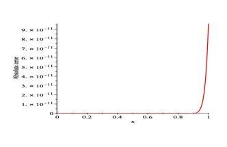
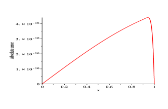
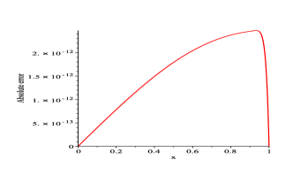
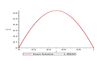
where $\theta$ is the solution of $\theta=\sqrt{2\lambda}\cosh\left(\theta/4\right)$. Using L-RKM for Eqs. (17)-(18), taking $x_{i}=\frac{i+0.3}{m}$,   $i=0,1,\,2,...,m-2$, the numerical solution $y_{m,n}\left(x\right)$ is calculated by Eq. (15). Comparison of L-RKM at some selected grid points with exact solution are given in Table 1, Table 4 and Table 7. Absolute error of different $m$ values for this example are given in Table 2, Table 5 and Table 8. Comparison of absolute error for different methods are given in Table 3 and Table 6. Absolute error of L-RKM solution for $y(x)$ and its derivatives are given in Fig. 1-5.

6 Conclusion

In this research, Legendre reproducing kernel method (L-RKM) is proposed and successfully applied to find the numerical solution of the fractional Bratu-type boundary value problems. Numerical results show that the present method is a powerful and effective for solving fractional Bratu-type boundary value problems. Furthermore, convergence of present iterative method is discussed.

Table 1: Numerical results for Example 5.1 with fractional order ($\lambda$=1, $m=20$ and $n=30$)

$x$	Exact Sol.	$\alpha$=2	$\alpha$=1.9	$\alpha$=1.8
0.1	0.04984679124541	0.04984679124541	0.053348029010	0.05640455239
0.2	0.08918993462882	0.08918993462882	0.094053979156	0.09778884381
0.3	0.11760909576794	0.11760909576794	0.122561203471	0.12577795186
0.4	0.13479025388418	0.13479025388418	0.139016612388	0.14107528890
0.5	0.14053921440047	0.14053921440047	0.143580804066	0.14424570594
0.6	0.13479025388418	0.13479025388418	0.136494883917	0.13586263427
0.7	0.11760909576794	0.11760909576794	0.118101177356	0.11655270867
0.8	0.08918993462882	0.08918993462882	0.088844712904	0.08700454024
0.9	0.04984679124541	0.04984679124541	0.049263971500	0.04796098207

Table 2: Absolute error of Example 5.1 for different $m$ values with $\lambda$=1, $n=30$ and $\alpha=2$

$x$	$m=10$	$m=12$	$m=14$	$m=16$	$m=18$
0.1	4.59E-10	1.25E-11	3.52E-13	1.01E-14	2.96E-16
0.2	8.17E-10	2.30E-11	6.62E-13	1.93E-14	5.68E-16
0.3	1.18E-9	3.34E-11	9.65E-13	2.82E-14	8.35E-16
0.4	1.53E-9	4.35E-11	1.25E-12	3.69E-14	1.09E-15
0.5	1.86E-9	5.30E-11	1.53E-12	4.51E-14	1.33E-15
0.6	2.17E-9	6.19E-11	1.79E-12	5.28E-14	1.56E-15
0.7	2.46E-9	7.02E-11	2.03E-12	5.99E-14	1.77E-15
0.8	2.72E-9	7.75E-11	2.25E-12	6.63E-14	1.96E-15
0.9	2.90E-9	8.44E-11	2.45E-12	7.22E-14	2.13E-15

Table 3: Absolute error of L-RKM and different methods for Example 5.1 case $\lambda=1$

$x$	B-Spline [6]	Laplace [7]	LGSM [8]	DM [11]	L-RKM
0.1	2.97E-6	1.97E-6	7.50E-7	2.68E-3	5.53E-17
0.2	5.46E-6	3.93E-6	1.01E-6	2.02E-3	1.09E-16
0.3	7.33E-6	5.85E-6	9.04E-7	1.52E-4	1.63E-16
0.4	8.49E-6	7.70E-6	5.23E-7	2.20E-3	2.15E-15
0.5	8.89E-6	9.46E-6	5.06E-9	3.01E-3	2.64E-15
0.6	8.49E-6	1.11E-5	5.13E-7	2.20E-3	3.11E-15
0.7	7.33E-6	1.25E-5	8.94E-7	1.52E-4	3.54E-15
0.8	5.46E-6	1.34E-5	1.00E-6	2.02E-3	3.92E-15
0.9	2.97E-6	1.19E-5	7.41E-7	2.68E-3	4.27E-15

Table 4: Numerical results for Example 5.1 with fractional order ($\lambda$=2, $m=20$ and $n=30$)

$x$	Exact Sol.	$\alpha$=2	$\alpha$=1.9	$\alpha$=1.8
0.1	0.11441074326774	0.11441074326804	0.12395416270	0.13161211082
0.2	0.20641911648760	0.20641911648819	0.22060766752	0.23047094173
0.3	0.27387931182555	0.27387931182641	0.28927167294	0.29804837485
0.4	0.31508936422566	0.31508936422678	0.32910866272	0.33469946332
0.5	0.32895242134111	0.32895242134245	0.33985942541	0.34125713685
0.6	0.31508936422566	0.31508936422720	0.32203437200	0.31930371842
0.7	0.27387931182555	0.27387931182723	0.27693051224	0.27114363748
0.8	0.20641911648760	0.20641911648939	0.20652983899	0.19963116013
0.9	0.11441074326774	0.11441074326959	0.11332086854	0.10793583205

Table 5: Absolute error of Example 5.1 for different $m$ values with $\lambda$=2, $n=30$ and $\alpha=2$

$x$	$m=10$	$m=12$	$m=14$	$m=16$	$m=18$
0.1	9.65E-8	6.25E-9	4.17E-10	2.84E-11	1.96E-12
0.2	1.76E-7	1.16E-8	7.92E-10	5.44E-11	3.78E-12
0.3	2.53E-7	1.69E-8	1.14E-9	7.91E-11	5.50E-12
0.4	3.24E-7	2.16E-8	1.47E-9	1.01E-10	7.08E-12
0.5	3.86E-7	2.58E-8	1.76E-9	1.21E-10	8.47E-12
0.6	4.37E-7	2.92E-8	1.99E-9	1.38E-10	9.62E-12
0.7	4.76E-7	3.19E-8	2.18E-9	1.50E-10	1.05E-11
0.8	5.02E-7	3.37E-8	2.30E-9	1.59E-10	1.11E-11
0.9	5.09E-7	3.48E-8	2.38E-9	1.64E-10	1.14E-11

Table 6: Absolute error of L-RKM and different methods for Example 5.1 case $\lambda=2$

$x$	B-Spline [6]	Laplace [7]	LGSM [8]	DM [11]	L-RKM
0.1	1.71E-5	2.12E-3	4.03E-6	1.52E-2	4.08E-13
0.2	3.25E-5	4.20E-3	5.70E-6	1.46E-2	8.04E-13
0.3	4.48E-5	6.18E-3	5.22E-6	5.88E-3	1.18E-12
0.4	5.28E-5	8.00E-3	3.07E-6	3.24E-3	1.52E-12
0.5	5.26E-5	9.59E-3	1.45E-8	6.98E-3	1.83E-12
0.6	5.28E-5	1.09E-2	3.04E-6	3.24E-3	2.08E-12
0.7	4.48E-5	1.19E-2	5.19E-6	5.88E-3	2.28E-12
0.8	3.25E-5	1.23E-2	5.67E-6	1.46E-2	2.42E-12
0.9	1.71E-5	1.08E-2	4.01E-6	1.52E-2	2.50E-12

Table 7: Numerical results for Example 5.1 with fractional order ($\lambda$=3, $m=20$ and $n=30$)

$x$	Exact Sol.	$\alpha$=2	$\alpha$=1.9	$\alpha$=1.8
0.1	0.21577498476753	0.21577498329811	0.24085457687	0.26065428735
0.2	0.39431958747803	0.39431958460834	0.43526223628	0.46414428666
0.3	0.52843643955821	0.52843643546802	0.57680617280	0.60602026500
0.4	0.61182920818459	0.61182920316127	0.65968880520	0.68206752260
0.5	0.64014669604146	0.64014669046258	0.68090952720	0.69191607740
0.6	0.61182920818459	0.61182920247466	0.64127386680	0.63986648210
0.7	0.52843643955821	0.52843643413164	0.54537595346	0.53412579803
0.8	0.39431958747803	0.39431958268710	0.40065374951	0.38508131538
0.9	0.21577498476753	0.21577498087398	0.21597352866	0.20346054571

Table 8: Absolute error of Example 5.1 for different $m$ values with $\lambda$=3, $n=30$ and $\alpha=2$

$x$	$m=10$	$m=12$	$m=14$	$m=16$	$m=18$
0.1	8.91E-6	1.14E-6	1.52E-7	1.97E-8	3.42E-9
0.2	1.67E-5	2.19E-6	2.93E-7	3.81E-8	6.63E-9
0.3	2.39E-5	3.13E-6	4.20E-7	5.49E-8	9.49E-9
0.4	2.99E-5	3.92E-6	5.27E-7	6.89E-8	1.17E-8
0.5	3.43E-5	4.50E-6	6.04E-7	7.93E-8	1.33E-8
0.6	3.67E-5	4.82E-6	6.47E-7	8.52E-8	1.40E-8
0.7	3.71E-5	4.87E-6	6.54E-7	8.67E-8	1.38E-8
0.8	3.56E-5	4.68E-6	6.28E-7	8.38E-8	1.28E-8
0.9	3.21E-5	4.29E-6	5.77E-7	7.74E-8	1.32E-8

Figure 1: The plot shows exact solution and L-RKM solution of Example 5.1 for $\alpha$=2, $\lambda=1$, $m=20$ and $n=30$ (on left), The plot shows absolute error of L-RKM solution of Example 5.1 for $\alpha$=2, $\lambda=1$, $m=20$ and $n=30$ (on right).

Figure 2: The plot shows absolute error of $y^{\prime}(x)$ for Example 5.1 with $\alpha$=2, $\lambda=1$, $m=20$ and $n=30$ (on left), The plot shows absolute error of $y^{\prime\prime}(x)$ for Example 5.1 with $\alpha$=2, $\lambda=1$, $m=20$ and $n=30$ (on right).

Figure 3: The plot shows absolute error of $y^{\prime\prime\prime}(x)$ for Example 5.1 with $\alpha$=2, $\lambda=1$, $m=20$ and $n=30$ (on left), The plot shows absolute error of $y^{(4)}(x)$ for Example 5.1 with $\alpha$=2, $\lambda=1$, $m=20$ and $n=30$ (on right).

Figure 4: The plot shows exact solution and L-RKM solution of Example 5.1 for $\alpha$=2, $\lambda=2$, $m=20$ and $n=30$ (on left), The plot shows absolute error of L-RKM solution of Example 5.1 for $\alpha$=2, $\lambda=2$, $m=20$ and $n=30$ (on right).

Figure 5: The plot shows exact solution and L-RKM solution of Example 5.1 for $\alpha$=2, $\lambda=3$, $m=20$ and $n=30$ (on left), The plot shows absolute error of L-RKM solution of Example 5.1 for $\alpha$=2, $\lambda=3$, $m=20$ and $n=30$ (on right).

References

• (1) Podlubny I (1999) Fractional differential equations, Academic Press, New York
• (2) Lakshmikantham V, Leela S, Vasundhara Devi J (2009) Theory of fractional dynamic systems, Cambridge Scientific Publishers
• (3) Sakar MG, Ergören H (2015) Alternative variational iteration method for solving the time-fractional Fornberg-Whitham equation, Appl Math Model 39(14):3972-3979
• (4) Sakar MG, Erdogan F (2013) The homotopy analysis method for solving the time-fractional Fornberg-Whitham equation and comparison with Adomian’s decomposition method, Appl Math Model 37(20):8876-8885
• (5) Inc M, Akgül A, Geng F (2015) Reproducing kernel Hilbert space method for solving Bratu’s problem, Bull Malays Math Sci Soc 38(1):271-287
• (6) Caglar H, Caglar N, Özer M, Valarıstos A, Anagnostopoulos AN (2010) B-spline method for solving Bratu’s problem, International Journal of Computer Mathematics 87(8):1885-1891
• (7) Khuri SA (2004) A new approach to Bratu’s problem, Applied Mathematics and Computation 147:131-136
• (8) Abbasbandy S, Hashemi MS, Liu CS (2011) The Lie-group shooting method for solving the Bratu equation, Commun Nonlinear Sci Numer Simulat 16:4238-4249
• (9) Li S, Liao SJ (2005) An analytic approach to solve multiple solutions of a strongly nonlinear problem, Appl Math Comput 169(2):854–865
• (10) Aregbesola YAS, Odejide SA (2005) A note on the Bratu problem, Math Sci Res J 9(9):236-243
• (11) Deeba E, Khuri SA, Xie S (2000) An algorithm for solving boundary value problems, Journal of Computational Physics 159:125-138
• (12) Aksoy Y, Pakdemirli M (2010) New perturbation-iteration solutions for Bratu-type equations, Computers and Mathematics with Applications 59:2802-2808
• (13) Zaremba S (1908) Sur le calcul numérique des fonctions demandées dans le probléme de Dirichlet et le problème hydrodynamique, Bulletin International de l’Académie des Sciences de Cracovie 1908:125-195
• (14) Xu MQ, Lin YZ, Wang YH (2016) A new algorithm for nonlinear fourth order multi-point boundary value problems, Applied Mathematics and Computation 274:163-168
• (15) Sakar MG (2017) Iterative reproducing kernel Hilbert spaces method for Riccati differential equations, Journal of Computational and Applied Mathematics 309:163-174
• (16) Chen Z, Zhou YF (2011) A new method for solving Hilbert type singular integral equations, Applied Mathematics and Computation 218:406-412
• (17) Babolian E, Javadi S, Moradi E (2016) RKM for solving Bratu-type differential equations of fractional order, Mathematical Methods in the Applied 39:1548-1557
• (18) Li X, Wu B (2017) A new reproducing kernel method for variable order fractional boundary value problems for functional differential equations, Journal of Computational and Applied Mathematics 311:387-393
• (19) Geng F (2011) A novel method for solving a class of singularly perturbed boundary value problems based on reproducing kernel method, Applied Mathematics and Computation 218:4211-4215
• (20) Jiang W, Lin Y (2010) Approximate solution of the fractional advection–dispersion equation, Computer Physics Communications 181(3):557-561
• (21) Sakar MG, Akgül A, Baleanu D (2017) On solutions of fractional Riccati differential equations, Adv Differ Equ (2017)39:1-10
• (22) Geng F, Cui M (2009) New method based on the HPM and RKHSM for solving forced Duffing equations with integral boundary conditions, Journal of Computational and Applied Mathematics 233(2):165-172
• (23) Khaleghi M, Babolian E, Abbasbandy S (2017) Chebyshev reproducing kernel method: application to two-point boundary value problems, Adv Differ Equ (2017)26:1-19
• (24) Sakar MG, Saldır O (2017) Improving variational iteration method with auxiliary parameter for nonlinear time-fractional partial differential equations, Journal of Optimization Theory and Applications 174(2):530-549
• (25) Jiang W, Tian T (2015) Numerical solution of nonlinear Volterra integro-differential equations of fractional order by the reproducing kernel method, Applied Mathematical Modelling 39(16):4871-4876
• (26) Diethelm K (2010) The analysis of fractional differential equations, Lecture notes in mathematics, Berlin Heidelberg, Springer-Verlag
• (27) Cui M, Lin Y (2009) Nonlinear Numerical Analysis in the Reproducing Kernel Space, Nova Science, New York