Faster Neural Network Training with Approximate Tensor Operations

Menachem Adelman
Intel & Technion
adelman.menachem@gmail.com
&Kfir Y. Levy
Technion
kfirylevy@technion.ac.il
&Ido Hakimi
Technion
idohakimi@gmail.com
&Mark Silberstein
Technion
mark@ee.technion.ac.il
A Viterbi fellow
Abstract

We propose a novel technique for faster deep neural network training which systematically applies sample-based approximation to the constituent tensor operations, i.e., matrix multiplications and convolutions. We introduce new sampling techniques, study their theoretical properties, and prove that they provide the same convergence guarantees when applied to SGD training. We apply approximate tensor operations to single and multi-node training of MLP and CNN networks on MNIST, CIFAR-10 and ImageNet datasets. We demonstrate up to 66% reduction in the amount of computations and communication, and up to 1.37x faster training time while maintaining negligible or no impact on the final test accuracy.

1 Introduction

Approximation techniques for faster inference and training of deep neural networks (DNNs) have received considerable attention. Examples include quantization  [1, 2, 3, 4, 5], low-rank and structured-sparse models [6, 7, 8, 9], weight extrapolations [10], and partial/asynchronous gradient updates in the context of distributed training  [11, 12]. Sampling-based approximations were used to accelerate inference [13, 14], but using them in training [15, 16, 17] has not been systematically studied nor demonstrated end-to-end GPU performance benefits in practice.

We propose a novel approach to accelerating DNN training by systematically approximating tensor operations via sampling. At a high level, the original matrix products and convolutions are replaced with their faster approximate versions. The approximation is applied separately to each tensor operation, keeping the network architecture and tensor dimensions intact, thereby facilitating the adoption of this technique in existing DNN training frameworks, potentially in combination with other approximation techniques. Furthermore, when combined with distributed training, our technique allows for seamless reduction in the communication bandwidth and increased performance gains.

We begin by reviewing the plethora of existing methods for approximating matrix multiplication. We compare several known algorithms [18, 19, 20, 21, 22, 23, 24, 25], and find column-row sampling (CRS) [20] to be the most suitable for approximating matrix multiplications in training. In order to compute the product of two matrices ABsuperscript𝐴top𝐵A^{\top}B, the CRS algorithm samples the columns of Asuperscript𝐴topA^{\top} and the corresponding rows of B𝐵B thus constructing smaller matrices which are then multiplied as usual. This method incurs low sampling overheads and lends itself to an efficient implementation using existing dense matrix product routines. CRS minimizes the approximation error for the Frobenius norm of the resulting matrix while keeping the approximation unbiased.

Sampling-based approximations can be interpreted as a form of Dropout  [26], and we discuss the similarities and differences between the two. While Dropout aims to prevent overfitting, we focus on approximations as means to accelerate training by reducing the amount of computation.

In this work we aim to answer two main questions. First, can neural networks be trained while using approximate tensor operations? Second, what are the relations between using exact or approximate operations during training?

We start by analyzing the simpler case of linear regression, where we can derive the effects of approximations in closed form. We define a new loss function that takes the sampling into account, and observe that the resulting gradients differ from the exact training due to the dependency between sampled features. To this end, we propose a new Bernoulli-CRS variant which achieves statistical independence of samples, study its properties, and show that in linear regression it is equivalent to dynamic L2subscript𝐿2L_{2} weight regularization of the original, non-approximate loss.

We then turn to the more general case of non-linear deep neural networks. We show that using sampling-based approximations in the backward pass provides the same convergence guarantees as the exact SGD for bounded weights. The convergence result holds for unbounded weights as well if approximation is applied only to the weight gradients and if the activation functions are bounded.

We also study a new TopK-CRS algorithm which deterministically selects the top-k𝑘k column-row pairs with the highest norms. We show that this algorithm is equivalent to the minimal mean square error estimator (MMSE) in case column-row pairs are pairwise independent with zero mean.

Last, we generalize matrix product approximation to convolutions and analyze the approximation error to derive the optimal sampling policy. This allows us to apply approximations to training of convolutional neural networks (CNNs).

We implement our techniques in PyTorch [27] 111https://github.com/acsl-technion/approx and evaluate them on several DNN topologies, including MLP and CNN networks on MNIST  [28], Wide ResNet 28-10  [29] on CIFAR-10  [30], and ResNet-50 and ResNet-152  [31] on ImageNet  [32]. We demonstrate up to 66% reduction in the number of FLOPs and up to 1.33x faster training time with little or no degradation in model accuracy.

We develop another flavor of TopK-CRS which samples according to the weight norms only. When sampling the same subset of weights for different workers in a data-parallel setting, our sampling technique enables reducing the amount of gradient communication between workers. Notably, our algorithm is compatible with the standard AllReduce approach used in distributed deep learning. We implement an AllReduce scheme that takes advantage of the smaller gradient footprint and demonstrate 1.09x-1.37x speedup in multi-node training.

Our contributions are as follows:

  • We derive general convergence guarantees for training with approximate tensor operations.

  • We develop novel sampling algorithms and analyze their theoretical properties.

  • We extend sampling-based algorithms to fast approximation of multi-channel convolutions.

  • We show that our approach can reduce the computation, communication and total training time on several popular neural network architectures with little or no accuracy degradation.

2 Related work

To the best of our knowledge, we are the first to study the application of sample-based approximations of tensor operations to speed up DNN training. However, there have been several prior efforts to accelerate DNN computations via approximation which we survey below.

Several works accelerate inference through model compression [33, 34, 35, 36, 37, 38, 39]. A large body of work is devoted to quantization and low-precision datatypes (see for example [1, 2, 5]). Approximation was used to extrapolate weight values [10]. Another approach enforces low-rank or structured-sparse structure on the layers, resulting in lower computational cost both for training and inference [6, 7, 8, 9]. Other works accelerate inference by approximating large matrices as products of lower-ranked ones [40, 41] or through locality-sensitive hashing [42].

In the context of distributed training, several works targeted communication bottlenecks by gradient quantization [3, 4], delayed weight updates [11, 12] and low-rank approximation of the gradient matrix [43]. These methods are complementary and compatible with ours.

Sampling-based approximations were used to accelerate inference [13, 14], but using them for training[15, 16, 17] has not been systematically studied nor shown to speed up training on GPUs without accuracy degradation. Sub-sampling whole layers was shown to enable training of very deep CNNs [44].

2.1 Approximate matrix multiplication

There are several known algorithms for approximating matrix product. However, only those that meet the following requirements will be effective for DNN training. First, the algorithm should apply to dense matrices of arbitrary dimensions. Second, to reduce training time, the overall multiplication including input transformation should be faster than the original product. Last, the algorithm should be amenable to efficient implementation on commodity hardware.

Using these criteria, we consider the following algorithms:

Random walk  [18] This algorithm performs random walks on a graph representation of the input matrices, but is applicable to non-negative matrices only.

Random projections  [22, 23, 21] The two matrices to be multiplied are first projected into a lower-dimensional subspace by a scaled random sign matrix. These algorithms require both input matrices to be roughly square, otherwise the cost of projection will be similar to the cost of original product. In DNNs, however, it is common for one dimension to be smaller than the other.

FFT  [24, 25] These algorithms represent each column-row outer product as a polynomial multiplication and then calculate it using Fast Fourier Transform. The complexity depends on the sparsity of the input matrices, decreasing as the sparsity increases. Therefore, these algorithms might not be effective for dense matrices.

SVD  [19, 33, 36] Several algorithms replace one input matrix with its low-rank approximation using truncated SVD. These algorithms are suitable for inference where the weight matrix factorization can be pre-computed offline, but are not applicable to training since the high cost of factorization is incurred in every matrix product.

Column-row sampling (CRS)  [19, 20] The sampling algorithm approximates matrix product ABsuperscript𝐴top𝐵A^{\top}B by sampling k𝑘k columns of Asuperscript𝐴topA^{\top} and respective rows of B𝐵B to form smaller matrices, which are then multiplied as usual.

We choose CRS as the basis for our current work because it meets all the criteria above: It is applicable to fully-connected layers of any size, its effectiveness does not depend on the matrix contents, its sampling is computationally lightweight, and may use regular matrix multiplication algorithms since the sampled sub-matrices remain dense.

2.2 CRS

Let An×m,Bn×pformulae-sequence𝐴superscript𝑛𝑚𝐵superscript𝑛𝑝A\in\mathbb{R}^{n\times m},B\in\mathbb{R}^{n\times p}. Their product ABsuperscript𝐴top𝐵A^{\top}B is approximated as a weighted sum of outer products between sampled columns of Asuperscript𝐴topA^{\top} and corresponding rows of B𝐵B:

ABt=1k1kpitA(it)B(it)superscript𝐴top𝐵superscriptsubscript𝑡1𝑘1𝑘subscript𝑝subscript𝑖𝑡superscript𝐴topsubscript𝑖𝑡subscript𝐵subscript𝑖𝑡\displaystyle A^{\top}B\approx\sum_{t=1}^{k}\frac{1}{kp_{i_{t}}}A^{\top(i_{t})}B_{(i_{t})} (1)

where A(i),B(i)superscript𝐴top𝑖subscript𝐵𝑖A^{\top(i)},B_{(i)} denote the matrix i𝑖i’th column and row respectively, k𝑘k is the number of samples (satisfying 1kn1𝑘𝑛1\leq k\leq n), {pi}i=1nsuperscriptsubscriptsubscript𝑝𝑖𝑖1𝑛\{p_{i}\}_{i=1}^{n} is a probability distribution over the column-row pairs of A,Bsuperscript𝐴top𝐵A^{\top},B and it{1,,n}subscript𝑖𝑡1𝑛i_{t}\in\left\{1,...,n\right\}. This algorithm allows linear reduction in complexity from O(mnp)𝑂𝑚𝑛𝑝O(mnp) to O(mkp)𝑂𝑚𝑘𝑝O(mkp).

(1) can also be expressed as ADSSDBsuperscript𝐴top𝐷superscript𝑆top𝑆𝐷𝐵A^{\top}DS^{\top}SDB, where Dn×n𝐷superscript𝑛𝑛D\in\mathbb{R}^{n\times n} is a diagonal scaling matrix with:

(D)j,j=1kpjsubscript𝐷𝑗𝑗1𝑘subscript𝑝𝑗\displaystyle(D)_{j,j}=\frac{1}{\sqrt{kp_{j}}} (2)

and Sk×n𝑆superscript𝑘𝑛S\in\mathbb{R}^{k\times n} is a sampling matrix that selects k𝑘k features, possibly with replacement. S𝑆S is a random matrix, where each row has 1 in one entry and zeros in others. In each row, the probability of having the non-zero entry in column j𝑗j is pjsubscript𝑝𝑗p_{j}.

Drineas et al. [20] show that CRS is unbiased:

𝔼[ADSSDB]=AB𝔼delimited-[]superscript𝐴top𝐷superscript𝑆top𝑆𝐷𝐵superscript𝐴top𝐵\displaystyle\mathbb{E}\left[{A^{\top}DS^{\top}SDB}\right]=A^{\top}B (3)

and also derive upper bounds for the expected Frobenius and spectral norms of the error matrix ABADSSDBnormsuperscript𝐴top𝐵superscript𝐴top𝐷superscript𝑆top𝑆𝐷𝐵\left|\left|A^{\top}B-A^{\top}DS^{\top}SDB\right|\right|. They show that the error is minimized when the sampling probabilities are proportional to the product of the column-row Euclidean norms:

pi=|A(i)||B(i)|j=1n|A(j)||B(j)|subscript𝑝𝑖subscript𝐴𝑖subscript𝐵𝑖superscriptsubscript𝑗1𝑛subscript𝐴𝑗subscript𝐵𝑗\displaystyle p_{i}=\frac{\lvert A_{(i)}\rvert\lvert B_{(i)}\rvert}{\sum_{j=1}^{n}\lvert A_{(j)}\rvert\lvert B_{(j)}\rvert} (4)

In which case the expected Frobenius error is:

1k(t=1k|A(it)||B(it)|)21kABF21𝑘superscriptsuperscriptsubscript𝑡1𝑘subscript𝐴subscript𝑖𝑡subscript𝐵subscript𝑖𝑡21𝑘superscriptsubscriptnormsuperscript𝐴top𝐵𝐹2\displaystyle\frac{1}{k}\left(\sum_{t=1}^{k}\lvert A_{(i_{t})}\rvert\lvert B_{(i_{t})}\rvert\right)^{2}-\frac{1}{k}\left|\left|A^{\top}B\right|\right|_{F}^{2} (5)

2.3 Approximate Tensor Operations and Dropout

Sampling-based approximations can be interpreted as a flavor of Dropout  [26], a popular technique to prevent overfitting by randomly zeroing individual activations during training. However, the sparsity pattern resulting from Dropout is unstructured and therefore cannot be exploited efficiently by GPUs despite recent advances in structured sparsity support[8]. Prior works on fast Dropout training [45, 46] are different than ours and do not demonstrate acceleration of large networks while maintaining accuracy.

Some works proposed non-uniform Dropout probabilities for individual activations [47] or full channels [48]. Their sampling heuristics are different from ours which are derived from optimal approximation. Furthermore, they use Dropout only for preventing overfitting and do not leverage it to speed up training. In our experiments we demonstrate the utility of sampling-based approximations for DNNs with and without Dropout. Conversely, we did not observe improved accuracy from approximations which could have been attributed to reduced overfitting.

3 Approximate Linear Regression

We now analyze CRS in the simpler context of linear regression, where we can derive the effects of approximations in closed form. We show that this leads to biased gradient estimates.

Let Xn×M𝑋superscript𝑛𝑀X\subset\mathbb{R}^{n\times M} a dataset containing M𝑀M examples, each a vector in nsuperscript𝑛\mathbb{R}^{n}. Every xiXsuperscript𝑥𝑖𝑋x^{i}\in X is associated with a "ground truth" value yisuperscript𝑦𝑖y^{i}\in\mathbb{R}.

Let wn𝑤superscript𝑛w\in\mathbb{R}^{n} be parameters in a linear model that predicts a value y¯isuperscript¯𝑦𝑖\bar{y}^{i}\in\mathbb{R} for every xiXsuperscript𝑥𝑖𝑋x^{i}\in X:

y¯i=wxisuperscript¯𝑦𝑖superscript𝑤topsuperscript𝑥𝑖\displaystyle\bar{y}^{i}=w^{\top}x^{i} (6)

To simplify the notation we do not include an explicit bias term. We do so without loss of generality since we can always add another entry of 111 to the features.

Let us define the MSE (Mean Square Error) loss function:

=i=1M(y¯iyi)2superscriptsubscript𝑖1𝑀superscriptsuperscript¯𝑦𝑖superscript𝑦𝑖2\displaystyle\ell=\sum_{i=1}^{M}(\bar{y}^{i}-y^{i})^{2} (7)

When using SGD (Stochastic Gradient Descent), we are given a single example xinsuperscript𝑥𝑖superscript𝑛x^{i}\in\mathbb{R}^{n} in each step, and update w𝑤w using the gradients w𝑤\frac{\partial\ell}{\partial w}. For notation simplicity we omit the superscript i𝑖i from xi,y¯i,yisuperscript𝑥𝑖superscript¯𝑦𝑖superscript𝑦𝑖x^{i},\bar{y}^{i},y^{i}.

The gradients are given by the chain rule as:

w𝑤\displaystyle\frac{\partial\ell}{\partial w} =2x(wxy)absent2𝑥superscript𝑤top𝑥𝑦\displaystyle=2x(w^{\top}x-y) (8)

Now, let us assume that the multiplication wxsuperscript𝑤top𝑥w^{\top}x is approximated using CRS. The linear regression model now becomes:

y^=wDSSDx^𝑦superscript𝑤top𝐷superscript𝑆top𝑆𝐷𝑥\displaystyle\hat{y}=w^{\top}DS^{\top}SDx (9)

and for the MSE loss the gradients will be:

w^=2DSSDx(wDSSDxy)^𝑤2𝐷superscript𝑆top𝑆𝐷𝑥superscript𝑤top𝐷superscript𝑆top𝑆𝐷𝑥𝑦\displaystyle\widehat{\frac{\partial\ell}{\partial w}}=2DS^{\top}SDx(w^{\top}DS^{\top}SDx-y) (10)

Where w^^𝑤\widehat{\frac{\partial\ell}{\partial w}} denotes the CRS weight gradients.

Note that DSSD𝐷superscript𝑆top𝑆𝐷DS^{\top}SD appears twice in (10). In wDSSDxsuperscript𝑤top𝐷superscript𝑆top𝑆𝐷𝑥w^{\top}DS^{\top}SDx it represents sampling in the forward pass, while in DSSDx𝐷superscript𝑆top𝑆𝐷𝑥DS^{\top}SDx it results in passing gradients only to the elements of w𝑤w that were sampled in the forward pass.

It should be emphasized that (9) and (10) in fact describe gradients with respect to a different loss function compared to (8): one loss function uses y^^𝑦\hat{y} while the other uses y¯¯𝑦\bar{y}. If the approximate gradients are unbiased estimates of the non-approximate gradients, we could relate the approximate training process to the original one. However, the weight gradients do not satisfy this unbiasedness property:

𝔼[(w^)j]=2xj(t=1nwt𝔼[(S~)j,j(S~)t,t]xty)𝔼delimited-[]subscript^𝑤𝑗2subscript𝑥𝑗superscriptsubscript𝑡1𝑛subscript𝑤𝑡𝔼delimited-[]subscript~𝑆𝑗𝑗subscript~𝑆𝑡𝑡subscript𝑥𝑡𝑦\displaystyle\mathbb{E}\left[{(\widehat{\frac{\partial\ell}{\partial w}})_{j}}\right]=2x_{j}\left(\sum_{t=1}^{n}w_{t}\mathbb{E}\left[{(\tilde{S})_{j,j}(\tilde{S})_{t,t}}\right]x_{t}-y\right) (11)

where we denote S~DSSD~𝑆𝐷superscript𝑆top𝑆𝐷\tilde{S}\triangleq DS^{\top}SD, and use the fact that S~~𝑆\tilde{S} is diagonal.

For the expression in (11) to be equal to that in (8) we need that 𝔼[(S~)j,j(S~)t,t]=1𝔼delimited-[]subscript~𝑆𝑗𝑗subscript~𝑆𝑡𝑡1\mathbb{E}\left[{(\tilde{S})_{j,j}(\tilde{S})_{t,t}}\right]=1. However, this is not the case because (S~)j,jsubscript~𝑆𝑗𝑗(\tilde{S})_{j,j} and (S~)t,tsubscript~𝑆𝑡𝑡(\tilde{S})_{t,t} are not independent random variables: an entry in the diagonal of S~~𝑆\tilde{S} is the (scaled) number of times a column-row pair was selected out of the k𝑘k total samples in CRS. The event of selecting a particular pair therefore affects selecting others.

We note that if instead of changing the loss function we treated the approximate multiplication as a "black box" that replaces the original product, we could use (8) and only replace the forward pass product wxsuperscript𝑤top𝑥w^{\top}x with the "black box" substitute of wDSSDxsuperscript𝑤top𝐷superscript𝑆top𝑆𝐷𝑥w^{\top}DS^{\top}SDx. This would yield:

w~=2x(wDSSDxy)~𝑤2𝑥superscript𝑤top𝐷superscript𝑆top𝑆𝐷𝑥𝑦\displaystyle\widetilde{\frac{\partial\ell}{\partial w}}=2x(w^{\top}DS^{\top}SDx-y) (12)

which satisfies:

𝔼[w~]=w.𝔼delimited-[]~𝑤𝑤\displaystyle\mathbb{E}\left[{\widetilde{\frac{\partial\ell}{\partial w}}}\right]=\frac{\partial\ell}{\partial w}. (13)

(12) is equivalent to applying the approximate computation in the forward pass, but propagating the gradients to all weight entries in the same way as if the computation were exact. In practice we find that this approach leads to significantly lower accuracy in deep neural networks compared to sampling the same entries in the forward and backward pass, or to applying approximations in the backward pass only.

4 Bernoulli-CRS

We now turn to develop Bernoulli-CRS, a new variant of sampling approximation that enables to sample column-row pairs independently and without replacement. Applied to linear regression, we show that using Bernoulli-CRS is equivalent to employing unbiased gradient estimates in addition to a bias term which can be interpreted as scale dependent weight regularization.

Bernoulli-CRS: These aforementioned properties can be achieved by assigning a separate Bernoulli sampling probability pisubscript𝑝𝑖p_{i} for each column-row pair i𝑖i, and sampling pairs independently of each other. To control the amount of sampling, we add another constraint that all the probabilities will sum up to an integer k𝑘k:

i=1npi=ksuperscriptsubscript𝑖1𝑛subscript𝑝𝑖𝑘\displaystyle\sum_{i=1}^{n}p_{i}=k (14)

Let us define Kn×n𝐾superscript𝑛𝑛K\in\mathbb{R}^{n\times n} a random diagonal sampling matrix where Kj,jBernoulli(pj)similar-tosubscript𝐾𝑗𝑗Bernoullisubscript𝑝𝑗K_{j,j}\sim\text{Bernoulli}(p_{j}) for 1jn1𝑗𝑛1\leq j\leq n. Furthermore, let us define another diagonal scaling matrix Pn×n𝑃superscript𝑛𝑛P\in\mathbb{R}^{n\times n} where Pj,j=1pjsubscript𝑃𝑗𝑗1subscript𝑝𝑗P_{j,j}=\frac{1}{\sqrt{p_{j}}} for 1jn1𝑗𝑛1\leq j\leq n.

Using the K𝐾K and P𝑃P matrices we may now define our new Bernoulli-CRS algorithm. Let An×m𝐴superscript𝑛𝑚A\in\mathbb{R}^{n\times m} and Bn×p𝐵superscript𝑛𝑝B\in\mathbb{R}^{n\times p}. The product ABsuperscript𝐴top𝐵A^{\top}B can be approximated with A~B~superscript~𝐴top~𝐵\tilde{A}^{\top}\tilde{B} defined as follows:

A~B~:=i=1nZipiA(i)B(i)=APKKPBassignsuperscript~𝐴top~𝐵superscriptsubscript𝑖1𝑛subscript𝑍𝑖subscript𝑝𝑖superscript𝐴top𝑖subscript𝐵𝑖superscript𝐴top𝑃𝐾𝐾𝑃𝐵\displaystyle\tilde{A}^{\top}\tilde{B}:=\sum_{i=1}^{n}\frac{Z_{i}}{p_{i}}A^{\top(i)}B_{(i)}=A^{\top}PKKPB (15)

where {ZiBernoulli(pi)}i=1nsuperscriptsubscriptsimilar-tosubscript𝑍𝑖Bernoullisubscript𝑝𝑖𝑖1𝑛\{Z_{i}\sim\text{Bernoulli}(p_{i})\}_{i=1}^{n} are independent random variables. We denote A~KPA~𝐴𝐾𝑃𝐴\tilde{A}\triangleq KPA and B~KPB~𝐵𝐾𝑃𝐵\tilde{B}\triangleq KPB.

In the appendix we develop the properties of Bernoulli-CRS. We show it is unbiased and derive bounds on the error variance both in expectation and in high probability. We derive the optimal sampling probabilities minimizing the expected variance, and show that under certain conditions they are given by the simpler expression:

pi=min{k|A(i)||B(i)|j=1n|A(j)||B(j)|,1}subscript𝑝𝑖𝑘subscript𝐴𝑖subscript𝐵𝑖superscriptsubscript𝑗1𝑛subscript𝐴𝑗subscript𝐵𝑗1\displaystyle p_{i}=\min\left\{\frac{k\lvert A_{(i)}\rvert\lvert B_{(i)}\rvert}{\sum_{j=1}^{n}\lvert A_{(j)}\rvert\lvert B_{(j)}\rvert},1\right\} (16)

In the appendix we show that applying Bernoulli-CRS in linear regression leads to unbiased estimate of the original gradients with an additional regularization term (w)𝑤\mathcal{R}(w), which we define as:

(w)𝑤\displaystyle\mathcal{R}(w) =𝐄[j=1n1pjpjxj2wj2]absent𝐄delimited-[]superscriptsubscript𝑗1𝑛1subscript𝑝𝑗subscript𝑝𝑗superscriptsubscript𝑥𝑗2superscriptsubscript𝑤𝑗2\displaystyle=\mathbf{E}\left[\sum_{j=1}^{n}\frac{1-p_{j}}{p_{j}}x_{j}^{2}w_{j}^{2}\right] (17)

and the expectation is with respect to the distribution of the data samples.

The term (w)𝑤\mathcal{R}(w) can be interpreted as input-dependent L2subscript𝐿2L_{2} regularization. The regularization is higher as xjsubscript𝑥𝑗x_{j} grows in magnitude and as pjsubscript𝑝𝑗p_{j} decreases. Both serve to reduce the impact on the weights if they were chosen with small probabilities or mostly because of the input size. We note that Wager et al. [49] conduct a similar analysis for Dropout in the particular case where the same sampling probability is used for all features.

To summarize, sampling in the simpler case of linear regression minimizes the original loss function with an added regularization term.

5 Approximate Backpropagation in Non-Linear Deep Networks

The analysis of approximate linear regression cannot simply generalize to deep non-linear networks: non-linearity leads to biased network output even if the approximate multiplication is itself unbiased. Still, we are able to obtain strong theoretical results on the relations between exact and approximate training if the approximations are limited to the backward pass: the forward pass is calculated as usual, and the matrix products in the backward pass are performed using approximate matrix multiplication.

We prove the following theorem:

Theorem 1.

Let f(x,W,b)𝑓𝑥𝑊𝑏f(x,W,b) be a multi-layer neural network with β𝛽\beta-Lipschitz activation functions σ𝜎\sigma. Let \ell be a β𝛽\beta-Lipschitz loss function, and let the network be trained with SGD using properly decreasing learning rate. Assume that the weights are bounded; and further assume that the matrix products in the backward pass are approximated using an unbiased approximation scheme, i.e.,

𝔼[AB𝚊𝚙𝚙𝚛𝚘𝚡(AB)]=0𝔼delimited-[]superscript𝐴top𝐵𝚊𝚙𝚙𝚛𝚘𝚡superscript𝐴top𝐵0\mathbb{E}\left[{A^{\top}B-\mathtt{approx}(A^{\top}B)}\right]=0

and that there exists a constant C𝐶C and a norm ||||\left|\left|\cdot\right|\right| such that:

𝔼[AB𝚊𝚙𝚙𝚛𝚘𝚡(AB)2]CA2B2.𝔼delimited-[]superscriptnormsuperscript𝐴top𝐵𝚊𝚙𝚙𝚛𝚘𝚡superscript𝐴top𝐵2𝐶superscriptnorm𝐴2superscriptnorm𝐵2\mathbb{E}\left[{\left|\left|A^{\top}B-\mathtt{approx}(A^{\top}B)\right|\right|^{2}}\right]\leq C\left|\left|A\right|\right|^{2}\left|\left|B\right|\right|^{2}.

Then the approximated NN gradient estimates are unbiased, and their second moments are bounded.

Corollary.

Based on recent works on non-convex optimization (see e.g.  [50]), the unbiasedness and bounded second moments ensured by Theorem 1 imply that approximate backpropagation enjoys the same convergence guarantees as regular SGD training.

In the appendix we show that CRS and other sampling algorithms satisfy the property

𝔼[AB𝚊𝚙𝚙𝚛𝚘𝚡(AB)2]CA2B2𝔼delimited-[]superscriptnormsuperscript𝐴top𝐵𝚊𝚙𝚙𝚛𝚘𝚡superscript𝐴top𝐵2𝐶superscriptnorm𝐴2superscriptnorm𝐵2\mathbb{E}\left[{\left|\left|A^{\top}B-\mathtt{approx}(A^{\top}B)\right|\right|^{2}}\right]\leq C\left|\left|A\right|\right|^{2}\left|\left|B\right|\right|^{2}

Note that for Theorem 1 we required that weights will be bounded during the training process. This is a strong assumption which could be justified if weight regularization or clipping is used. In the appendix we prove the same results without relying on these assumptions, if only the weight gradients are approximated and if the activation function is bounded (such as sigmoid).

6 Sampling Without Scaling and Top-k𝑘k Selection

We now consider a different sampling scheme where k𝑘k column-row pairs are selected deterministically without scaling. This can be viewed as a special case of Bernoulli-CRS, where the sampling probabilities are either 0 or 1. We now show that under certain assumptions on the distribution of the input matrices, this scheme can lead to the optimal estimation:

Theorem 2.

Let A𝐴A be an n×m𝑛𝑚n\times m random matrix and B𝐵B be an n×p𝑛𝑝n\times p random matrix, such that

𝔼[A(i)B(i)]=0𝔼delimited-[]superscript𝐴top𝑖subscript𝐵𝑖0\mathbb{E}\left[{A^{\top(i)}B_{(i)}}\right]=0

for 1in1𝑖𝑛1\leq i\leq n. Assume k𝑘k column-row pairs with indices {j}1nsuperscriptsubscript𝑗1𝑛\{j\}_{1}^{n} are sampled from A𝐴A and B𝐵B. Then, the MMSE estimator of the product ABsuperscript𝐴top𝐵A^{\top}B is A~B~superscript~𝐴top~𝐵\tilde{A}^{\top}\tilde{B} where A~,B~~𝐴~𝐵\tilde{A},\tilde{B} are constructed from the sampled column-row pairs without scaling.

Furthermore, if A(i)B(i)superscript𝐴top𝑖subscript𝐵𝑖A^{\top(i)}B_{(i)} and A(j)B(j)superscript𝐴top𝑗subscript𝐵𝑗A^{\top(j)}B_{(j)} are independent for different i,j𝑖𝑗i,j then the MSE is minimized when sampling k𝑘k pairs with the maximum norm multiplication |A(i)||B(i)|subscript𝐴𝑖subscript𝐵𝑖\lvert A_{(i)}\rvert\lvert B_{(i)}\rvert.

The assumptions in Theorem 2 can hold in practice if weights are initialized with a zero-centered distribution[51], if the distribution of weights remains centered around zero during training [51, 52, 53, 54], and if different weights can be considered pairwise-independent [55].

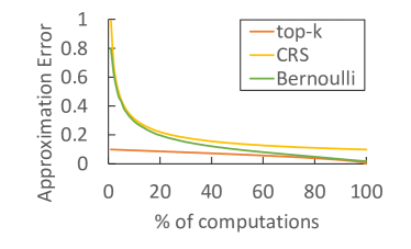
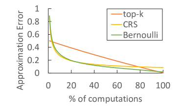
We study the approximation quality of CRS, Bernoulli-CRS and top-k𝑘k selection on synthetic matrix multiplication. We generate 100×100100100100\times 100 random matrices and compute the error metric:

AB𝚊𝚙𝚙𝚛𝚘𝚡(AB)FAFBFsubscriptnormsuperscript𝐴top𝐵𝚊𝚙𝚙𝚛𝚘𝚡superscript𝐴top𝐵𝐹subscriptnorm𝐴𝐹subscriptnorm𝐵𝐹\displaystyle\frac{\left|\left|A^{\top}B-\mathtt{approx}(A^{\top}B)\right|\right|_{F}}{\left|\left|A\right|\right|_{F}\left|\left|B\right|\right|_{F}} (18)

Figures 1(a),1(b) show the approximation error for different algorithms and sampling ratios, averaged over 1000 runs. We observe that Bernoulli-CRS outperforms CRS in higher sampling ratios. Also, when one matrix has i.i.d entries with zero mean, Bernoulli-CRS outperforms CRS and top-k𝑘k selection performs the best as expected from Theorem 2.
Refer to caption
(a) Matrix product: both matrix entries drawn from 𝒩(1,1)𝒩11\mathcal{N}(1,1)
Refer to caption
(b) Matrix product: one matrix entries drawn from 𝒩(0,1)𝒩01\mathcal{N}(0,1), the other from 𝒩(1,1)𝒩11\mathcal{N}(1,1)
Figure 1: Approximation error depending on the amount of performed computations. Lower is better.

We also consider a different flavor of top-k𝑘k selection, which we refer to as "top-k𝑘k-weights": sampling k𝑘k column-row pairs corresponding to rows of B𝐵B with the highest norms. While not providing the theoretical guarantees of Theorem 2, the new variant has a desirable property for data parallel distributed training, where weights are identical between different workers. A deterministic selection algorithm that only depends on the weights will sample the same weights for all workers, allowing to reduce the gradient communication between nodes to the selected weights only.

7 Approximating Convolutions

We extend the basic CRS algorithm to the approximation of multi-channel convolutions. In matrix multiplication sampling is performed over the common dimension. The analogue for multi-channel convolution is to sample over the input channels dimension, illustrated in Figure 2. As in the matrix case, the output dimensions remain the same.

Refer to caption
Figure 2: Sampling one input channel out of three

In the appendix we derive the optimal sampling probabilities and scaling factors. Bernoulli-CRS and top-k𝑘k algorithms can be developed for convolutions as well in an analogous way.

8 Experimental Results

We implement CRS, Bernoulli-CRS and top-k𝑘k selection approximation algorithms in PyTorch both for matrix multiplication and convolution. Our implementation allows to control the sampling degree and the application of approximation in the forward or backward passes.

We replace exact tensor operations with their sampling-based approximations, without changing training hyper-parameters. Only column-row pairs sampled in the forward pass are used during backpropagation as the rest do not affect the loss. Hence, sampling in the forward pass also reduces the amount of backward pass computations by the same ratio. We apply approximations only during training, and use exact computations for validation/test evaluation.

We evaluate our approximate training technique on several network architectures and datasets: MLP and CNN on MNIST, Wide ResNet 28-10 on CIFAR-10 and ResNet-50 and ResNet-152 on ImageNet. We train the networks on a single node using NVidia V100 GPUs (two GPUs for ResNet-152, one for the rest), and measure the reduction in multiply-accumulate operations due to sampling as well as the overall speedup in total training time versus the non-approximate baseline. The appendix includes additional details on the models and the training process.

Table 1: Compute reduction, communication reduction and wall-clock speedup of training with approximate tensor operations.

Network Compute Communication Accuracy Training
Reduction Reduction (Baseline) Speedup
MLP (MNIST) 50% - 98.22% (98.22%) -
CNN (MNIST) 66% - 99.25% (99.35%) -
WRN-28-10 (CIFAR-10) 50% - 95.89% (96.17%) 1.33x
ResNet-50 (ImageNet) 6.5% - 75.63% (75.6%) 1.04x
ResNet-152 Single Node 40% - 76.44% (77.65%) 1.16x
9% - 77.66% (77.65%) 1.04x
(ImageNet) 8 Nodes 40% 48% 76.44% (77.65%) 1.37x
12% 23% 77.48% (77.65%) 1.13x
9% 13% 77.8% (77.65%) 1.09x
Refer to caption
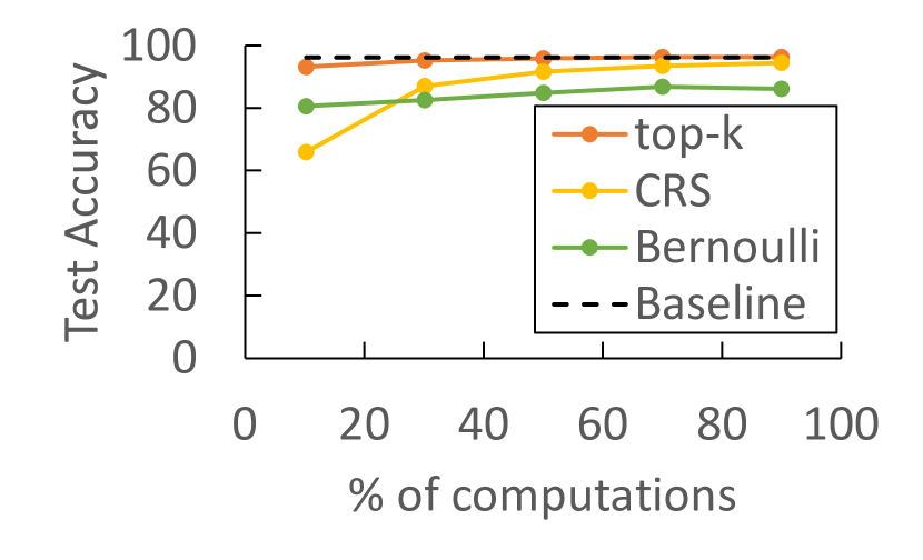
Figure 3: WRN-28-10 on CIFAR-10 (approximate forward and backward)
Refer to caption
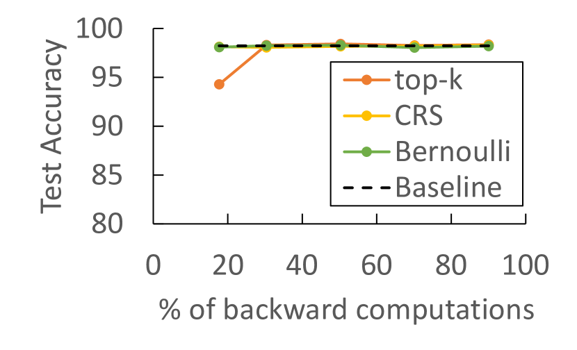
Figure 4: 3-layer MLP on MNIST (exact forward, approximate backward)
Refer to caption
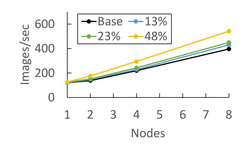
Figure 5: AllReduce with top-k-weights sampling (% fewer gradients sent).

Our results using top-k𝑘k sampling are summarized in Table 1. We see a reduction of up to 66% in the computational cost with little or no degradation in model accuracy, and up to 1.33x faster training time. We believe the gap between compute reduction and end-to-end speedup can be reduced by fusing the sampling with the matrix multiplication routines, or running on a different HW architecture that allows fast sampling and norm computation. We note that the small MNIST models do not exhibit training time speedup since they are not compute-intensive enough to saturate the GPU. The ratio between compute reduction and actual speedup is smaller in ResNet-152 compared to ResNet-50 and WRN-28-10 because the batch size per GPU is lower due to the limited GPU memory capacity.

Sampling Algorithms

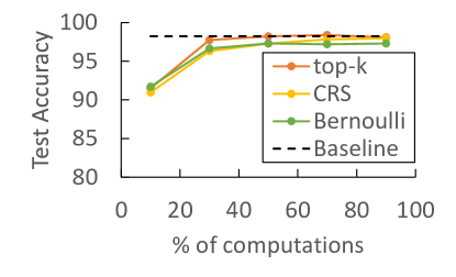
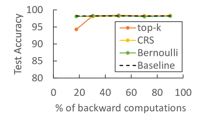
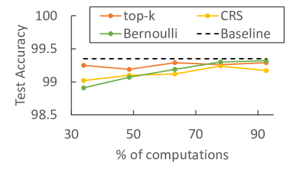
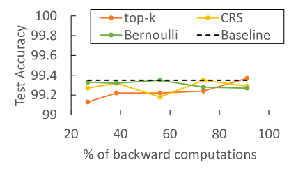
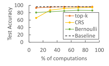
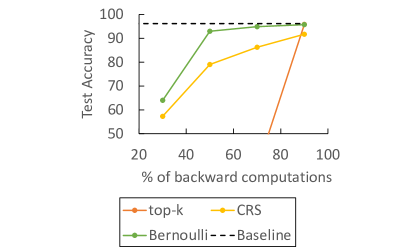
We compare CRS, Bernoulli-CRS and top-k𝑘k selection on MNIST and CIFAR-10 and find empirically that top-k𝑘k results in higher accuracy and faster training time (Figure 5). This result is consistent with that of approximate 𝒩(0,1)𝒩01\mathcal{N}(0,1) matrix product (Figure 1(b)). This is not surprising given Theorem 2 and our empirical observation that the weight distribution is close to symmetrical around zero throughout training.

Approximations in Forward Pass and Backpropagation

For the small MNIST models we are able to perform as low as 10% of the computations in the backward pass without harming accuracy (Fig. 5). However, in the larger models (WRN-28-10) we find empirically that accuracy drops when approximating only the backward pass. Therefore, in Table 1 we report results for consistent sampling in the forward and backward passes.

Sampling Ratio Sensitivity

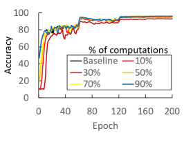
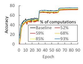
We find that the achievable compute reduction is not consistent across networks and datasets. For MNIST and CIFAR-10 we maintain good accuracy while reducing 50%-66% of the computations. However, ImageNet proved to be more sensitive and we kept the accuracy intact when applying 50% sampling to the ResNet layers with 1024 or more channels only. Figure 6 shows the learning curves under different sampling ratios compared to the non-approximate baseline.
Refer to caption
(a) WRN-28-10 CIFAR-10
Refer to caption
(b) ResNet-50 Imagenet (top-1)
Refer to caption
(c) ResNet-152 Imagenet (top-1)
Figure 6: Learning curves for validation accuracy under different top-k𝑘k sampling ratios

Distributed Training

We implement an AllReduce "top-k𝑘k-weights" scheme in PyTorch. This scheme performs reduction only for the gradients of the sampled weights, reducing inter-node communications. Table 1 shows the accuracy-speedup trade-off for ResNet-152 distributed training. Figure 5 shows the respective scaling behavior of these schemes relative to the exact baseline. We note that compute savings did not lead to significant single-node speedup since in this experiment the V100 GPUs (from Amazon AWS) had lower memory capacity, which led to smaller batch size per GPU. The multi-node training speedup is therefore mostly due to the communication savings.

9 Conclusion

In this work we have demonstrated the utility of sample-based approximation of tensor operations for neural network training, both theoretically and empirically. We believe that further acceleration could be achieved through dedicated GPU primitives fusing sampling and matrix multiplication/convolution, as well as varying and adaptive sampling rates for different layers and iterations. Studying other approximation algorithms, applications in resource-constrained environments and bridging the gaps between our theoretical results and what worked best in practice are all promising directions for future research. Overall, we believe that sample-based approximations and fast approximations in general are valuable additions to the toolbox of techniques for deep learning acceleration.

Acknowledgments and Disclosure of Funding

K.Y. Levy acknowledges support from the Israel Science Foundation (grant No. 447/20). I. Hakimi acknowledges support from the Hasso Plattner Institute at the Technion. M. Silberstein acknowledges support from the Israel Science Foundation (grant No. 1027/18).

References

  • Hubara et al. [2016] Itay Hubara, Matthieu Courbariaux, Daniel Soudry, Ran El-Yaniv, and Yoshua Bengio. Quantized neural networks: Training neural networks with low precision weights and activations. arXiv preprint arXiv:1609.07061, 2016.
  • Micikevicius et al. [2017] Paulius Micikevicius, Sharan Narang, Jonah Alben, Gregory Diamos, Erich Elsen, David Garcia, Boris Ginsburg, Michael Houston, Oleksii Kuchaev, Ganesh Venkatesh, et al. Mixed precision training. arXiv preprint arXiv:1710.03740, 2017.
  • Seide et al. [2014] Frank Seide, Hao Fu, Jasha Droppo, Gang Li, and Dong Yu. 1-bit stochastic gradient descent and its application to data-parallel distributed training of speech dnns. In Fifteenth Annual Conference of the International Speech Communication Association, 2014.
  • Wen et al. [2017] Wei Wen, Cong Xu, Feng Yan, Chunpeng Wu, Yandan Wang, Yiran Chen, and Hai Li. Terngrad: Ternary gradients to reduce communication in distributed deep learning. In Advances in Neural Information Processing Systems, pages 1508–1518, 2017.
  • Chakrabarti and Moseley [2019] Ayan Chakrabarti and Benjamin Moseley. Backprop with approximate activations for memory-efficient network training. Advances in Neural Information Processing Systems, 32:2429–2438, 2019.
  • Mamalet and Garcia [2012] Franck Mamalet and Christophe Garcia. Simplifying convnets for fast learning. In International Conference on Artificial Neural Networks, pages 58–65. Springer, 2012.
  • Kuchaiev and Ginsburg [2017] Oleksii Kuchaiev and Boris Ginsburg. Factorization tricks for lstm networks. arXiv preprint arXiv:1703.10722, 2017.
  • Mishra et al. [2021] Asit Mishra, Jorge Albericio Latorre, Jeff Pool, Darko Stosic, Dusan Stosic, Ganesh Venkatesh, Chong Yu, and Paulius Micikevicius. Accelerating sparse deep neural networks. arXiv preprint arXiv:2104.08378, 2021.
  • Hubara et al. [2021] Itay Hubara, Brian Chmiel, Moshe Island, Ron Banner, Seffi Naor, and Daniel Soudry. Accelerated sparse neural training: A provable and efficient method to find n: m transposable masks. arXiv preprint arXiv:2102.08124, 2021.
  • Kamarthi and Pittner [1999] Sagar V Kamarthi and Stefan Pittner. Accelerating neural network training using weight extrapolations. Neural networks, 12(9):1285–1299, 1999.
  • Recht et al. [2011] Benjamin Recht, Christopher Re, Stephen Wright, and Feng Niu. Hogwild: A lock-free approach to parallelizing stochastic gradient descent. In Advances in neural information processing systems, pages 693–701, 2011.
  • Strom [2015] Nikko Strom. Scalable distributed dnn training using commodity gpu cloud computing. In Sixteenth Annual Conference of the International Speech Communication Association, 2015.
  • Hua et al. [2019] Weizhe Hua, Yuan Zhou, Christopher M De Sa, Zhiru Zhang, and G Edward Suh. Channel gating neural networks. In Advances in Neural Information Processing Systems, pages 1886–1896, 2019.
  • Gao et al. [2018] Xitong Gao, Yiren Zhao, Łukasz Dudziak, Robert Mullins, and Cheng-zhong Xu. Dynamic channel pruning: Feature boosting and suppression. arXiv preprint arXiv:1810.05331, 2018.
  • Sun et al. [2017a] Xu Sun, Xuancheng Ren, Shuming Ma, and Houfeng Wang. meprop: Sparsified back propagation for accelerated deep learning with reduced overfitting. In International Conference on Machine Learning, pages 3299–3308, 2017a.
  • Chen et al. [2019] Beidi Chen, Tharun Medini, James Farwell, Sameh Gobriel, Charlie Tai, and Anshumali Shrivastava. Slide: In defense of smart algorithms over hardware acceleration for large-scale deep learning systems. arXiv preprint arXiv:1903.03129, 2019.
  • Goli and Aamodt [2020] Negar Goli and Tor M Aamodt. Resprop: Reuse sparsified backpropagation. In Proceedings of the IEEE/CVF Conference on Computer Vision and Pattern Recognition, pages 1548–1558, 2020.
  • Cohen and Lewis [1999] Edith Cohen and David D Lewis. Approximating matrix multiplication for pattern recognition tasks. Journal of Algorithms, 30(2):211–252, 1999.
  • Drineas and Kannan [2001] Petros Drineas and Ravi Kannan. Fast monte-carlo algorithms for approximate matrix multiplication. In FoCS, volume 1, pages 452–459, 2001.
  • Drineas et al. [2006] Petros Drineas, Ravi Kannan, and Michael W Mahoney. Fast monte carlo algorithms for matrices i: Approximating matrix multiplication. SIAM Journal on Computing, 36(1):132–157, 2006.
  • Magen and Zouzias [2011] Avner Magen and Anastasios Zouzias. Low rank matrix-valued chernoff bounds and approximate matrix multiplication. In Proceedings of the twenty-second annual ACM-SIAM symposium on Discrete Algorithms, pages 1422–1436. SIAM, 2011.
  • Sarlos [2006] Tamas Sarlos. Improved approximation algorithms for large matrices via random projections. In Foundations of Computer Science, 2006. FOCS’06. 47th Annual IEEE Symposium on, pages 143–152. IEEE, 2006.
  • Clarkson and Woodruff [2009] Kenneth L Clarkson and David P Woodruff. Numerical linear algebra in the streaming model. In Proceedings of the forty-first annual ACM symposium on Theory of computing, pages 205–214. ACM, 2009.
  • Pagh [2013] Rasmus Pagh. Compressed matrix multiplication. ACM Transactions on Computation Theory (TOCT), 5(3):9, 2013.
  • Kutzkov [2013] Konstantin Kutzkov. Deterministic algorithms for skewed matrix products. In 30th International Symposium on Theoretical Aspects of Computer Science, page 466, 2013.
  • Srivastava et al. [2014] Nitish Srivastava, Geoffrey Hinton, Alex Krizhevsky, Ilya Sutskever, and Ruslan Salakhutdinov. Dropout: A simple way to prevent neural networks from overfitting. The Journal of Machine Learning Research, 15(1):1929–1958, 2014.
  • Paszke et al. [2019] Adam Paszke, Sam Gross, Francisco Massa, Adam Lerer, James Bradbury, Gregory Chanan, Trevor Killeen, Zeming Lin, Natalia Gimelshein, Luca Antiga, et al. Pytorch: An imperative style, high-performance deep learning library. In Advances in neural information processing systems, pages 8026–8037, 2019.
  • LeCun et al. [1998] Yann LeCun, Léon Bottou, Yoshua Bengio, and Patrick Haffner. Gradient-based learning applied to document recognition. Proceedings of the IEEE, 86(11):2278–2324, 1998.
  • Zagoruyko and Komodakis [2016] Sergey Zagoruyko and Nikos Komodakis. Wide residual networks. arXiv preprint arXiv:1605.07146, 2016.
  • Krizhevsky and Hinton [2009] Alex Krizhevsky and Geoffrey Hinton. Learning multiple layers of features from tiny images. 2009.
  • He et al. [2016] Kaiming He, Xiangyu Zhang, Shaoqing Ren, and Jian Sun. Deep residual learning for image recognition. In Proceedings of the IEEE conference on computer vision and pattern recognition, pages 770–778, 2016.
  • Russakovsky et al. [2015] Olga Russakovsky, Jia Deng, Hao Su, Jonathan Krause, Sanjeev Satheesh, Sean Ma, Zhiheng Huang, Andrej Karpathy, Aditya Khosla, Michael Bernstein, et al. Imagenet large scale visual recognition challenge. International journal of computer vision, 115(3):211–252, 2015.
  • Denton et al. [2014] Emily L Denton, Wojciech Zaremba, Joan Bruna, Yann LeCun, and Rob Fergus. Exploiting linear structure within convolutional networks for efficient evaluation. In Advances in neural information processing systems, pages 1269–1277, 2014.
  • Jaderberg et al. [2014] Max Jaderberg, Andrea Vedaldi, and Andrew Zisserman. Speeding up convolutional neural networks with low rank expansions. In Proceedings of the British Machine Vision Conference. BMVA Press, 2014.
  • Lebedev et al. [2014] Vadim Lebedev, Yaroslav Ganin, Maksim Rakhuba, Ivan Oseledets, and Victor Lempitsky. Speeding-up convolutional neural networks using fine-tuned cp-decomposition. arXiv preprint arXiv:1412.6553, 2014.
  • Osawa et al. [2017] Kazuki Osawa, Akira Sekiya, Hiroki Naganuma, and Rio Yokota. Accelerating matrix multiplication in deep learning by using low-rank approximation. In High Performance Computing & Simulation (HPCS), 2017 International Conference on, pages 186–192. IEEE, 2017.
  • Gong et al. [2014] Yunchao Gong, Liu Liu, Ming Yang, and Lubomir Bourdev. Compressing deep convolutional networks using vector quantization. arXiv preprint arXiv:1412.6115, 2014.
  • Han et al. [2015a] Song Han, Huizi Mao, and William J Dally. Deep compression: Compressing deep neural networks with pruning, trained quantization and huffman coding. arXiv preprint arXiv:1510.00149, 2015a.
  • Sun et al. [2017b] Xu Sun, Xuancheng Ren, Shuming Ma, Bingzhen Wei, Wei Li, and Houfeng Wang. Training simplification and model simplification for deep learning: A minimal effort back propagation method. arXiv preprint arXiv:1711.06528, 2017b.
  • Choromanski et al. [2020] Krzysztof Choromanski, Valerii Likhosherstov, David Dohan, Xingyou Song, Andreea Gane, Tamas Sarlos, Peter Hawkins, Jared Davis, Afroz Mohiuddin, Lukasz Kaiser, et al. Rethinking attention with performers. arXiv preprint arXiv:2009.14794, 2020.
  • Wang et al. [2020] Sinong Wang, Belinda Li, Madian Khabsa, Han Fang, and Hao Ma. Linformer: Self-attention with linear complexity. arXiv preprint arXiv:2006.04768, 2020.
  • Kitaev et al. [2020] Nikita Kitaev, Łukasz Kaiser, and Anselm Levskaya. Reformer: The efficient transformer. arXiv preprint arXiv:2001.04451, 2020.
  • Vogels et al. [2019] Thijs Vogels, Sai Praneeth Karimireddy, and Martin Jaggi. Powersgd: Practical low-rank gradient compression for distributed optimization. arXiv preprint arXiv:1905.13727, 2019.
  • Huang et al. [2016] Gao Huang, Yu Sun, Zhuang Liu, Daniel Sedra, and Kilian Q Weinberger. Deep networks with stochastic depth. In European conference on computer vision, pages 646–661. Springer, 2016.
  • Wang and Manning [2013] Sida Wang and Christopher Manning. Fast dropout training. In international conference on machine learning, pages 118–126. PMLR, 2013.
  • Graham et al. [2015] Ben Graham, Jeremy Reizenstein, and Leigh Robinson. Efficient batchwise dropout training using submatrices. arXiv preprint arXiv:1502.02478, 2015.
  • Li et al. [2016] Zhe Li, Boqing Gong, and Tianbao Yang. Improved dropout for shallow and deep learning. In Advances in Neural Information Processing Systems, pages 2523–2531, 2016.
  • Hou and Wang [2019] Saihui Hou and Zilei Wang. Weighted channel dropout for regularization of deep convolutional neural network. In Proceedings of the AAAI Conference on Artificial Intelligence, volume 33, pages 8425–8432, 2019.
  • Wager et al. [2013] Stefan Wager, Sida Wang, and Percy S Liang. Dropout training as adaptive regularization. In Advances in neural information processing systems, pages 351–359, 2013.
  • Ge et al. [2015] Rong Ge, Furong Huang, Chi Jin, and Yang Yuan. Escaping from saddle points—online stochastic gradient for tensor decomposition. In Conference on Learning Theory, pages 797–842, 2015.
  • Glorot and Bengio [2010] Xavier Glorot and Yoshua Bengio. Understanding the difficulty of training deep feedforward neural networks. In Proceedings of the thirteenth international conference on artificial intelligence and statistics, pages 249–256. JMLR Workshop and Conference Proceedings, 2010.
  • Blundell et al. [2015] Charles Blundell, Julien Cornebise, Koray Kavukcuoglu, and Daan Wierstra. Weight uncertainty in neural network. In International Conference on Machine Learning, pages 1613–1622. PMLR, 2015.
  • Han et al. [2015b] Song Han, Jeff Pool, John Tran, and William J Dally. Learning both weights and connections for efficient neural networks. arXiv preprint arXiv:1506.02626, 2015b.
  • Thoma [2017] Martin Thoma. Analysis and optimization of convolutional neural network architectures. arXiv preprint arXiv:1707.09725, 2017.
  • Huang et al. [2020] Zhongzhan Huang, Wenqi Shao, Xinjiang Wang, and Ping Luo. Convolution-weight-distribution assumption: Rethinking the criteria of channel pruning. arXiv preprint arXiv:2004.11627, 2020.
  • Bertsekas and Tsitsiklis [1996] Dimitri P Bertsekas and John N Tsitsiklis. Neuro-dynamic programming. Athena Scientific, 1996.
  • Tropp [2012] Joel A Tropp. User-friendly tail bounds for sums of random matrices. Foundations of computational mathematics, 12(4):389–434, 2012.
  • Kingma and Ba [2014] Diederik P Kingma and Jimmy Ba. Adam: A method for stochastic optimization. arXiv preprint arXiv:1412.6980, 2014.

Appendices

Appendix A Bernoulli-CRS Properties

Let us define Kn×n𝐾superscript𝑛𝑛K\in\mathbb{R}^{n\times n} a random diagonal sampling matrix where Kj,jBernoulli(pj)similar-tosubscript𝐾𝑗𝑗Bernoullisubscript𝑝𝑗K_{j,j}\sim\text{Bernoulli}(p_{j}) for 1jn1𝑗𝑛1\leq j\leq n.

Let us define another diagonal scaling matrix Pn×n𝑃superscript𝑛𝑛P\in\mathbb{R}^{n\times n} where Pj,j=1pjsubscript𝑃𝑗𝑗1subscript𝑝𝑗P_{j,j}=\frac{1}{\sqrt{p_{j}}} for 1jn1𝑗𝑛1\leq j\leq n.

Using the K𝐾K and P𝑃P matrices we may now define our new Bernoulli-CRS algorithm. Let An×m𝐴superscript𝑛𝑚A\in\mathbb{R}^{n\times m} and Bn×p𝐵superscript𝑛𝑝B\in\mathbb{R}^{n\times p}. The product ABsuperscript𝐴top𝐵A^{\top}B can be approximated with A~B~superscript~𝐴top~𝐵\tilde{A}^{\top}\tilde{B} defined as follows:

A~B~:=i=1kZipiA(i)B(i)=APKKPBassignsuperscript~𝐴top~𝐵superscriptsubscript𝑖1𝑘subscript𝑍𝑖subscript𝑝𝑖superscript𝐴top𝑖subscript𝐵𝑖superscript𝐴top𝑃𝐾𝐾𝑃𝐵\displaystyle\tilde{A}^{\top}\tilde{B}:=\sum_{i=1}^{k}\frac{Z_{i}}{p_{i}}A^{\top(i)}B_{(i)}=A^{\top}PKKPB (19)

where {ZiBernoulli(pi)}i=1nsuperscriptsubscriptsimilar-tosubscript𝑍𝑖Bernoullisubscript𝑝𝑖𝑖1𝑛\{Z_{i}\sim\text{Bernoulli}(p_{i})\}_{i=1}^{n} are independent random variables. We denote A~KPA~𝐴𝐾𝑃𝐴\tilde{A}\triangleq KPA and B~KPB~𝐵𝐾𝑃𝐵\tilde{B}\triangleq KPB.

First, we show that the above holds in expectation:

Proposition 1.

𝔼[A~B~]=AB𝔼delimited-[]superscript~𝐴top~𝐵superscript𝐴top𝐵\mathbb{E}\left[{\tilde{A}^{\top}\tilde{B}}\right]=A^{\top}B.

Let T=Trace(K)𝑇Trace𝐾T=\text{Trace}(K) the number of non-zero diagonal elements in K𝐾K. We note that to perform the actual computation it is enough to sample the T𝑇T column-row pair with the corresponding element in K𝐾K being non-zero. Unlike CRS, the lower rank of the sampled matrices is not constant and depends on the random matrix K𝐾K. Its expectation is controlled through the parameter k𝑘k:

Proposition 2.

𝔼[T]=k𝔼delimited-[]𝑇𝑘\mathbb{E}\left[{T}\right]=k.

Therefore, Bernoulli-CRS will perform on average the same amount of computations as in the fixed-rank CRS.

Let us further derive the properties of the proposed sampling algorithm. Specifically, what are the optimal values for the probabilities pisubscript𝑝𝑖p_{i} under the constraint i=1npi=ksuperscriptsubscript𝑖1𝑛subscript𝑝𝑖𝑘\sum_{i=1}^{n}p_{i}=k?

First, let us calculate the variance of A~B~superscript~𝐴top~𝐵\tilde{A}^{\top}\tilde{B}:

Proposition 3.
𝐕𝐚𝐫[(A~B~)i,j]=t=1n1ptptAt,i2Bt,j2𝐕𝐚𝐫delimited-[]subscriptsuperscript~𝐴top~𝐵𝑖𝑗superscriptsubscript𝑡1𝑛1subscript𝑝𝑡subscript𝑝𝑡superscriptsubscript𝐴𝑡𝑖2superscriptsubscript𝐵𝑡𝑗2\mathbf{Var}\left[{(\tilde{A}^{\top}\tilde{B})_{i,j}}\right]=\sum_{t=1}^{n}\frac{1-p_{t}}{p_{t}}A_{t,i}^{2}B_{t,j}^{2}

We will be interested in the Frobenius norm of the error matrix ABA~B~F2superscriptsubscriptnormsuperscript𝐴top𝐵superscript~𝐴top~𝐵𝐹2\left|\left|A^{\top}B-\tilde{A}^{\top}\tilde{B}\right|\right|_{F}^{2}, which can be derived from the following theorem:

Theorem 3.

The expected Frobenius norm of the error matrix 𝔼[ABA~B~F2]𝔼delimited-[]superscriptsubscriptnormsuperscript𝐴top𝐵superscript~𝐴top~𝐵𝐹2\mathbb{E}\left[{\left|\left|A^{\top}B-\tilde{A}^{\top}\tilde{B}\right|\right|_{F}^{2}}\right] is t=1n1ptpt|A(t)|2|B(t)|2superscriptsubscript𝑡1𝑛1subscript𝑝𝑡subscript𝑝𝑡superscriptsubscript𝐴𝑡2superscriptsubscript𝐵𝑡2\sum_{t=1}^{n}\frac{1-p_{t}}{p_{t}}\lvert A_{(t)}\rvert^{2}\lvert B_{(t)}\rvert^{2}.

Furthermore, under the constraint i=1npi=ksuperscriptsubscript𝑖1𝑛subscript𝑝𝑖𝑘\sum_{i=1}^{n}p_{i}=k it is minimized for the probabilities:

pi=|A(i)||B(i)|μ1{0<|A(i)||B(i)|<μ}+1{|A(i)||B(i)|μ}subscript𝑝𝑖subscript𝐴𝑖subscript𝐵𝑖𝜇subscript10subscript𝐴𝑖subscript𝐵𝑖𝜇subscript1subscript𝐴𝑖subscript𝐵𝑖𝜇p_{i}=\frac{\lvert A_{(i)}\rvert\lvert B_{(i)}\rvert}{\sqrt{\mu}}1_{\{0<\lvert A_{(i)}\rvert\lvert B_{(i)}\rvert<\mu\}}+1_{\{\lvert A_{(i)}\rvert\lvert B_{(i)}\rvert\geq\mu\}}

where μ𝜇\mu is a root of the following function:

G(μ):=i=1n(|A(i)||B(i)|μ1{0<|A(i)||B(i)|<μ}+1{|A(i)||B(i)|μ})kassign𝐺𝜇superscriptsubscript𝑖1𝑛subscript𝐴𝑖subscript𝐵𝑖𝜇subscript10subscript𝐴𝑖subscript𝐵𝑖𝜇subscript1subscript𝐴𝑖subscript𝐵𝑖𝜇𝑘G(\mu):=\sum_{i=1}^{n}\left(\frac{\lvert A_{(i)}\rvert\lvert B_{(i)}\rvert}{\sqrt{\mu}}1_{\{0<\lvert A_{(i)}\rvert\lvert B_{(i)}\rvert<\mu\}}+1_{\{\lvert A_{(i)}\rvert\lvert B_{(i)}\rvert\geq\mu\}}\right)-k
Corollary.

The sampling probabilities

pi=min{k|A(i)||B(i)|j=1n|A(j)||B(j)|,1}subscript𝑝𝑖𝑘subscript𝐴𝑖subscript𝐵𝑖superscriptsubscript𝑗1𝑛subscript𝐴𝑗subscript𝐵𝑗1\displaystyle p_{i}=\min\left\{\frac{k\lvert A_{(i)}\rvert\lvert B_{(i)}\rvert}{\sum_{j=1}^{n}\lvert A_{(j)}\rvert\lvert B_{(j)}\rvert},1\right\}

are optimal if ki=1n|A(i)||B(i)|maxi|A(i)||B(i)|𝑘superscriptsubscript𝑖1𝑛subscript𝐴𝑖subscript𝐵𝑖subscript𝑖subscript𝐴𝑖subscript𝐵𝑖k\leq\frac{\sum_{i=1}^{n}\lvert A_{(i)}\rvert\lvert B_{(i)}\rvert}{\max_{i}\lvert A_{(i)}\rvert\lvert B_{(i)}\rvert}

From Theorem 3 it follows that for the probabilities:

pi=min{k|A(i)||B(i)|j=1n|A(j)||B(j)|,1}subscript𝑝𝑖𝑘subscript𝐴𝑖subscript𝐵𝑖superscriptsubscript𝑗1𝑛subscript𝐴𝑗subscript𝐵𝑗1\displaystyle p_{i}=\min\left\{\frac{k\lvert A_{(i)}\rvert\lvert B_{(i)}\rvert}{\sum_{j=1}^{n}\lvert A_{(j)}\rvert\lvert B_{(j)}\rvert},1\right\} (20)

the expected Frobenius error is:

1k(i=1nei|A(i)||B(i)|)2i=1nei|A(i)|2|B(i)|21𝑘superscriptsuperscriptsubscript𝑖1𝑛subscript𝑒𝑖subscript𝐴𝑖subscript𝐵𝑖2superscriptsubscript𝑖1𝑛subscript𝑒𝑖superscriptsubscript𝐴𝑖2superscriptsubscript𝐵𝑖2\displaystyle\frac{1}{k}\left(\sum_{i=1}^{n}e_{i}\lvert A_{(i)}\rvert\lvert B_{(i)}\rvert\right)^{2}-\sum_{i=1}^{n}e_{i}\lvert A_{(i)}\rvert^{2}\lvert B_{(i)}\rvert^{2} (21)

where we denote:

ei{1|A(i)||B(i)|j=1n|A(j)||B(j)|k0else.subscript𝑒𝑖cases1subscript𝐴𝑖subscript𝐵𝑖superscriptsubscript𝑗1𝑛subscript𝐴𝑗subscript𝐵𝑗𝑘0else\displaystyle e_{i}\triangleq\begin{cases}1&\lvert A_{(i)}\rvert\lvert B_{(i)}\rvert\leq\frac{\sum_{j=1}^{n}\lvert A_{(j)}\rvert\lvert B_{(j)}\rvert}{k}\\ 0&\text{else}\end{cases}. (22)

Comparing that with the bound in (5), we can see that different values of A,B𝐴𝐵A,B determine which algorithm performs better.

Knowing the expected Frobenius error also implies a bound on the spectral norm of the error matrix, since the spectral and Frobenius norms are related by:

AAFrAnorm𝐴subscriptnorm𝐴𝐹𝑟norm𝐴\displaystyle\left|\left|A\right|\right|\leq\left|\left|A\right|\right|_{F}\leq\sqrt{r}\left|\left|A\right|\right| (23)

where r𝑟r is the rank of A𝐴A and Anorm𝐴\left|\left|A\right|\right| denotes its spectral norm.

The following theorem yields high probability bounds for the Frobenius and spectral norms for the Bernoulli-CRS algorithm:

Theorem 4.

Let An×m𝐴superscript𝑛𝑚A\in\mathbb{R}^{n\times m} and Bn×p𝐵superscript𝑛𝑝B\in\mathbb{R}^{n\times p}. Let A~,B~~𝐴~𝐵\tilde{A},\tilde{B} be the sampled matrices according to the Bernoulli-CRS algorithm described above. Denote

RmaxiA(i)B(i)𝑅subscript𝑖normsuperscript𝐴top𝑖subscript𝐵𝑖R\triangleq\max_{i}\left|\left|A^{\top(i)}B_{(i)}\right|\right|

and

σ21k(i=1nei|A(i)||B(i)|)2i=1nei|A(i)|2|B(i)|2superscript𝜎21𝑘superscriptsuperscriptsubscript𝑖1𝑛subscript𝑒𝑖subscript𝐴𝑖subscript𝐵𝑖2superscriptsubscript𝑖1𝑛subscript𝑒𝑖superscriptsubscript𝐴𝑖2superscriptsubscript𝐵𝑖2\sigma^{2}\triangleq\frac{1}{k}\left(\sum_{i=1}^{n}e_{i}\lvert A_{(i)}\rvert\lvert B_{(i)}\rvert\right)^{2}-\sum_{i=1}^{n}e_{i}\lvert A_{(i)}\rvert^{2}\lvert B_{(i)}\rvert^{2}

then, for all t0𝑡0t\geq 0:

{ABA~B~t}(m+p)exp(t2/2σ2+Rt/3)normsuperscript𝐴top𝐵superscript~𝐴top~𝐵𝑡𝑚𝑝superscript𝑡22superscript𝜎2𝑅𝑡3\mathbb{P}\left\{\left|\left|A^{\top}B-\tilde{A}^{\top}\tilde{B}\right|\right|\geq t\right\}\leq(m+p)\cdot\exp\left(\frac{-t^{2}/2}{\sigma^{2}+Rt/3}\right)
{ABA~B~Ft}(m+p)3/2exp(t2/2σ2+Rt/3)subscriptnormsuperscript𝐴top𝐵superscript~𝐴top~𝐵𝐹𝑡superscript𝑚𝑝32superscript𝑡22superscript𝜎2𝑅𝑡3\mathbb{P}\left\{\left|\left|A^{\top}B-\tilde{A}^{\top}\tilde{B}\right|\right|_{F}\geq t\right\}\leq(m+p)^{3/2}\cdot\exp\left(\frac{-t^{2}/2}{\sigma^{2}+Rt/3}\right)

A.1 Bernoulli-CRS in linear regression

We now show that applying Bernoulli-CRS in linear regression leads to unbiased estimate of the original gradients with an additional term that can be interpreted as regularization. The analysis for linear regression using Bernoulli-CRS is the same as in Section 3, with the sampling and scaling matrices DSSD𝐷superscript𝑆top𝑆𝐷DS^{\top}SD replaced with PKKP𝑃𝐾𝐾𝑃PKKP

The expression for the weight gradient (simimlar to (11)) now becomes:

𝔼[(w^)j]=2xj(t=1nwt(𝔼[(K~)j,j(K~)t,t]xty)\displaystyle\mathbb{E}\left[{(\widehat{\frac{\partial\ell}{\partial w}})_{j}}\right]=2x_{j}(\sum_{t=1}^{n}w_{t}(\mathbb{E}\left[{(\tilde{K})_{j,j}(\tilde{K})_{t,t}}\right]x_{t}-y) (24)
=2xj(wxy+wj(𝔼[(K~)j,j2]1)xj)absent2subscript𝑥𝑗superscript𝑤top𝑥𝑦subscript𝑤𝑗𝔼delimited-[]superscriptsubscript~𝐾𝑗𝑗21subscript𝑥𝑗\displaystyle=2x_{j}(w^{\top}x-y+w_{j}\left(\mathbb{E}\left[{(\tilde{K})_{j,j}^{2}}\right]-1\right)x_{j}) (25)
=2xj(wxy+1pjpjwjxj)absent2subscript𝑥𝑗superscript𝑤top𝑥𝑦1subscript𝑝𝑗subscript𝑝𝑗subscript𝑤𝑗subscript𝑥𝑗\displaystyle=2x_{j}(w^{\top}x-y+\frac{1-p_{j}}{p_{j}}w_{j}x_{j}) (26)

where we denote K~PKKP~𝐾𝑃𝐾𝐾𝑃\tilde{K}\triangleq PKKP.

When comparing (26) and (8) we see that using Bernoulli-CRS yields unbiased estimates of the original gradients with an additional bias term that is related to a scale-dependent regularization (w)𝑤\mathcal{R}(w), which we define as:

(w)𝑤\displaystyle\mathcal{R}(w) =𝐄[j=1n1pjpjxj2wj2]absent𝐄delimited-[]superscriptsubscript𝑗1𝑛1subscript𝑝𝑗subscript𝑝𝑗superscriptsubscript𝑥𝑗2superscriptsubscript𝑤𝑗2\displaystyle=\mathbf{E}\left[\sum_{j=1}^{n}\frac{1-p_{j}}{p_{j}}x_{j}^{2}w_{j}^{2}\right] (27)

and the expectation is with respect to the distribution of the data samples.

This term can be interpreted as input-dependent L2subscript𝐿2L_{2} regularization. The regularization is higher as xjsubscript𝑥𝑗x_{j} grows in magnitude and as pjsubscript𝑝𝑗p_{j} decreases. Both serve to reduce the impact on the weights if they were chosen with small probabilities or mostly because of the input size.

Appendix B Approximating Convolutions - Details

Formally, let IB×IHIW×IC𝐼subscriptsuperscript𝐼𝑊𝐼𝐶𝐵𝐼𝐻I\in\mathbb{R}^{IW\times IC}_{B\times IH} be the input tensor, where B𝐵B is the batch size, IH,IW𝐼𝐻𝐼𝑊IH,IW are the input height and width, and IC𝐼𝐶IC are the input channels. Let KKH×KWIC×OC𝐾superscriptsubscript𝐾𝐻𝐾𝑊𝐼𝐶𝑂𝐶K\in\mathbb{R}_{KH\times KW}^{IC\times OC} be the kernels tensor, where KH,KW𝐾𝐻𝐾𝑊KH,KW are the kernel height and width, and IC,OC𝐼𝐶𝑂𝐶IC,OC are the input and output channels respectively. Let OB×OHOW×OC𝑂subscriptsuperscript𝑂𝑊𝑂𝐶𝐵𝑂𝐻O\in\mathbb{R}^{OW\times OC}_{B\times OH} be the output tensor, where OH,OW𝑂𝐻𝑂𝑊OH,OW are the output height and width.

The multi-channel convolution operation is defined as:

Ob,ohow,oc=IK=i=1ICkh=1KHkw=1KWIb,oh+kh1ow+kw1,iKkh,kwi,ocsuperscriptsubscript𝑂𝑏𝑜𝑜𝑤𝑜𝑐𝐼𝐾superscriptsubscript𝑖1𝐼𝐶superscriptsubscript𝑘1𝐾𝐻superscriptsubscript𝑘𝑤1𝐾𝑊superscriptsubscript𝐼𝑏𝑜𝑘1𝑜𝑤𝑘𝑤1𝑖superscriptsubscript𝐾𝑘𝑘𝑤𝑖𝑜𝑐\displaystyle O_{b,oh}^{ow,oc}=I*K=\sum_{i=1}^{IC}\sum_{kh=1}^{KH}\sum_{kw=1}^{KW}I_{b,oh+kh-1}^{ow+kw-1,i}\cdot K_{kh,kw}^{i,oc} (28)

For notation simplicity, we assume zero padding. The inner sums in (28) can be written as 1-channel convolutions:

Ob,ohow,oc=i=1ICI[i]K[i]superscriptsubscript𝑂𝑏𝑜𝑜𝑤𝑜𝑐superscriptsubscript𝑖1𝐼𝐶superscript𝐼delimited-[]𝑖subscript𝐾delimited-[]𝑖\displaystyle O_{b,oh}^{ow,oc}=\sum_{i=1}^{IC}I^{[i]}*K_{[i]} (29)

where I[i]B×IHIW×1superscript𝐼delimited-[]𝑖subscriptsuperscript𝐼𝑊1𝐵𝐼𝐻I^{[i]}\in\mathbb{R}^{IW\times 1}_{B\times IH} denotes a tensor with one input channel that corresponds to the i𝑖i’th input channel of I𝐼I, i.e I[i]b,ihiw,1=Ib,ihiw,isuperscriptsubscriptsuperscript𝐼delimited-[]𝑖𝑏𝑖𝑖𝑤1superscriptsubscript𝐼𝑏𝑖𝑖𝑤𝑖{I^{[i]}}_{b,ih}^{iw,1}=I_{b,ih}^{iw,i}. Similarly, K[i]KH×KW1×OCsubscript𝐾delimited-[]𝑖subscriptsuperscript1𝑂𝐶𝐾𝐻𝐾𝑊K_{[i]}\in\mathbb{R}^{1\times OC}_{KH\times KW} corresponds to the i𝑖i’th input channel of K𝐾K.

This formulation immediately hints at the possibility to sample over the input channel dimension, similarly to sampling column-row pairs in matrices. We propose to approximate convolutions by sampling lower-rank tensors:

O~=t=1k1kpitI[it]K[it]I~K~~𝑂superscriptsubscript𝑡1𝑘1𝑘subscript𝑝subscript𝑖𝑡superscript𝐼delimited-[]subscript𝑖𝑡subscript𝐾delimited-[]subscript𝑖𝑡~𝐼~𝐾\displaystyle\tilde{O}=\sum_{t=1}^{k}\frac{1}{kp_{i_{t}}}I^{[i_{t}]}*K_{[i_{t}]}\triangleq\tilde{I}*\tilde{K} (30)

where {it}t=1ksuperscriptsubscriptsubscript𝑖𝑡𝑡1𝑘\{i_{t}\}_{t=1}^{k} are such that it{1,,IC}subscript𝑖𝑡1𝐼𝐶i_{t}\in\{1,...,IC\} and {pi}i=1ICsuperscriptsubscriptsubscript𝑝𝑖𝑖1𝐼𝐶\{p_{i}\}_{i=1}^{IC} is a probability distribution over the input channels, I~~𝐼\tilde{I} is a tensor composed of sampled input channels of I𝐼I scaled by 1kpi1𝑘subscript𝑝𝑖\sqrt{\frac{1}{kp_{i}}}, and K~~𝐾\tilde{K} is a tensor composed of corresponding sampled input channels of K𝐾K scaled by the same factor.

Computing the convolution of the smaller tensors I~K~~𝐼~𝐾\tilde{I}*\tilde{K} can be done using standard efficient convolution implementations. Figure 2 illustrates the sampling operation.

The properties of the approximation in (30) can be derived similarly to the CRS derivations for matrix multiplication. In particular, we prove the approximation is unbiased, and similar to matrix CRS, we use sampling probabilities proportional to the tensor Euclidean norms:

pi=I[i]FK[i]Fj=1ICI[j]FK[j]Fsubscript𝑝𝑖subscriptnormsuperscript𝐼delimited-[]𝑖𝐹subscriptnormsubscript𝐾delimited-[]𝑖𝐹superscriptsubscript𝑗1𝐼𝐶subscriptnormsuperscript𝐼delimited-[]𝑗𝐹subscriptnormsubscript𝐾delimited-[]𝑗𝐹\displaystyle p_{i}=\frac{\big{\|}I^{[i]}\big{\|}_{F}\cdot\big{\|}K_{[i]}\big{\|}_{F}}{\sum_{j=1}^{IC}\big{\|}I^{[j]}\big{\|}_{F}\cdot\big{\|}K_{[j]}\big{\|}_{F}} (31)

In section C.4 we show that the optimal sampling probabilities are significantly more complicated to calculate, but under certain conditions they reduce to (31).

Bernoulli-CRS and top-k𝑘k algorithms can be developed for convolutions as well in an analogous way.

Appendix C Proofs

C.1 Proofs for Section 5 - Approximate Backpropagation

Theorem 1.

Let f(x,W,b)𝑓𝑥𝑊𝑏f(x,W,b) be a multi-layer neural network with β𝛽\beta-Lipschitz activation functions σ𝜎\sigma. Let \ell be a β𝛽\beta-Lipschitz loss function, and let the network be trained with SGD using properly decreasing learning rate. If the matrix products in the backward pass are approximated using an unbiased approximation scheme satisfying:

𝔼[AB𝚊𝚙𝚙𝚛𝚘𝚡(AB)]=0𝔼delimited-[]superscript𝐴top𝐵𝚊𝚙𝚙𝚛𝚘𝚡superscript𝐴top𝐵0\mathbb{E}\left[{A^{\top}B-\mathtt{approx}(A^{\top}B)}\right]=0

and:

𝔼[AB𝚊𝚙𝚙𝚛𝚘𝚡(AB)2]CA2B2𝔼delimited-[]superscriptnormsuperscript𝐴top𝐵𝚊𝚙𝚙𝚛𝚘𝚡superscript𝐴top𝐵2𝐶superscriptnorm𝐴2superscriptnorm𝐵2\mathbb{E}\left[{\left|\left|A^{\top}B-\mathtt{approx}(A^{\top}B)\right|\right|^{2}}\right]\leq C\left|\left|A\right|\right|^{2}\left|\left|B\right|\right|^{2}

for some finite constant C𝐶C and some norm ||||\left|\left|\cdot\right|\right|,

and if the weights are bounded, then the approximated gradients are unbiased with bounded second moments.

Corollary.

Based on recent works on non-convex optimization [50], Theorem 1 implies that approximate backpropagation enjoys the same convergence guarantees as regular SGD training.

Proof.

The network f𝑓f can be described by:

h1subscript1\displaystyle h_{1} =W1x+b1absentsuperscriptsubscript𝑊1top𝑥subscript𝑏1\displaystyle=W_{1}^{\top}x+b_{1}
a1subscript𝑎1\displaystyle a_{1} =σ(h1)absent𝜎subscript1\displaystyle=\sigma(h_{1})
hlsubscript𝑙\displaystyle h_{l} =Wlal1+blabsentsuperscriptsubscript𝑊𝑙topsubscript𝑎𝑙1subscript𝑏𝑙\displaystyle=W_{l}^{\top}a_{l-1}+b_{l}
alsubscript𝑎𝑙\displaystyle a_{l} =σ(hl)absent𝜎subscript𝑙\displaystyle=\sigma(h_{l})
y^^𝑦\displaystyle\hat{y} =WLaL1absentsuperscriptsubscript𝑊𝐿topsubscript𝑎𝐿1\displaystyle=W_{L}^{\top}a_{L-1}

where xn𝑥superscript𝑛x\in\mathbb{R}^{n},W1n×d1subscript𝑊1superscript𝑛subscript𝑑1W_{1}\in\mathbb{R}^{n\times{d_{1}}}, Wldl1×dlsubscript𝑊𝑙superscriptsubscript𝑑𝑙1subscript𝑑𝑙W_{l}\in\mathbb{R}^{d_{l-1}\times{d_{l}}}, bldlsubscript𝑏𝑙superscriptsubscript𝑑𝑙b_{l}\in\mathbb{R}^{d_{l}}, \ell is the number of layers and y^dL^𝑦superscriptsubscript𝑑𝐿\hat{y}\in\mathbb{R}^{d_{L}} is the network output.

Let us denote the weight, bias and activation gradients with respect to a loss function \ell by Wl,bl,alsubscript𝑊𝑙subscript𝑏𝑙subscript𝑎𝑙\nabla W_{l},\nabla b_{l},\nabla a_{l} respectively. Let us denote and the gradients yielded by the approximation scheme as W~l,b~l,a~lsubscript~𝑊𝑙subscript~𝑏𝑙subscript~𝑎𝑙\nabla\tilde{W}_{l},\nabla\tilde{b}_{l},\nabla\tilde{a}_{l}.

Lemma 1.
𝔼[W~l]=Wland𝔼[b~l]=blformulae-sequence𝔼delimited-[]subscript~𝑊𝑙subscript𝑊𝑙and𝔼delimited-[]subscript~𝑏𝑙subscript𝑏𝑙\mathbb{E}\left[{\nabla\tilde{W}_{l}}\right]=\nabla W_{l}\quad\text{and}\quad\mathbb{E}\left[{\nabla\tilde{b}_{l}}\right]=\nabla b_{l}
Proof.

We prove by induction. The last layer satisfies:

WL=aL1y^aL1=WLy^formulae-sequencesubscript𝑊𝐿subscript𝑎𝐿1^𝑦subscript𝑎𝐿1subscript𝑊𝐿^𝑦\displaystyle\nabla W_{L}=a_{L-1}\nabla\hat{y}\quad\quad\quad\nabla a_{L-1}=W_{L}\nabla\hat{y}

and its approximation is given by:

W~L=𝚊𝚙𝚙𝚛𝚘𝚡(aL1y^)a~L1=𝚊𝚙𝚙𝚛𝚘𝚡(WLy^)formulae-sequencesubscript~𝑊𝐿𝚊𝚙𝚙𝚛𝚘𝚡subscript𝑎𝐿1^𝑦subscript~𝑎𝐿1𝚊𝚙𝚙𝚛𝚘𝚡subscript𝑊𝐿^𝑦\displaystyle\nabla\tilde{W}_{L}=\mathtt{approx}(a_{L-1}\nabla\hat{y})\quad\quad\quad\nabla\tilde{a}_{L-1}=\mathtt{approx}(W_{L}\nabla\hat{y})

Since the approximation methods satisfies:

𝔼[AB𝚊𝚙𝚙𝚛𝚘𝚡(AB)]=0𝔼delimited-[]superscript𝐴top𝐵𝚊𝚙𝚙𝚛𝚘𝚡superscript𝐴top𝐵0\mathbb{E}\left[{A^{\top}B-\mathtt{approx}(A^{\top}B)}\right]=0

we get:

𝔼[W~L]=WL𝔼[a~L1]=aL1formulae-sequence𝔼delimited-[]subscript~𝑊𝐿subscript𝑊𝐿𝔼delimited-[]subscript~𝑎𝐿1subscript𝑎𝐿1\displaystyle\mathbb{E}\left[{\nabla\tilde{W}_{L}}\right]=\nabla W_{L}\quad\quad\quad\mathbb{E}\left[{\nabla\tilde{a}_{L-1}}\right]=\nabla a_{L-1}

for the induction step, we will show that if 𝔼[a~l]=al𝔼delimited-[]subscript~𝑎𝑙subscript𝑎𝑙\mathbb{E}\left[{\nabla\tilde{a}_{l}}\right]=\nabla a_{l} then:

𝔼[W~l1]𝔼delimited-[]subscript~𝑊𝑙1\displaystyle\mathbb{E}\left[{\nabla\tilde{W}_{l-1}}\right] =Wl1absentsubscript𝑊𝑙1\displaystyle=\nabla W_{l-1}
𝔼[b~l1]𝔼delimited-[]subscript~𝑏𝑙1\displaystyle\mathbb{E}\left[{\nabla\tilde{b}_{l-1}}\right] =bl1absentsubscript𝑏𝑙1\displaystyle=\nabla b_{l-1}
𝔼[a~l1]𝔼delimited-[]subscript~𝑎𝑙1\displaystyle\mathbb{E}\left[{\nabla\tilde{a}_{l-1}}\right] =al1absentsubscript𝑎𝑙1\displaystyle=\nabla a_{l-1}

W~l1subscript~𝑊𝑙1\nabla\tilde{W}_{l-1} is given by:

W~l1=𝚊𝚙𝚙𝚛𝚘𝚡(al1h~l)=𝚊𝚙𝚙𝚛𝚘𝚡(al1Σ(hl)a~l)subscript~𝑊𝑙1𝚊𝚙𝚙𝚛𝚘𝚡subscript𝑎𝑙1superscriptsubscript~𝑙top𝚊𝚙𝚙𝚛𝚘𝚡subscript𝑎𝑙1superscriptΣsubscript𝑙superscriptsubscript~𝑎𝑙top\nabla\tilde{W}_{l-1}=\mathtt{approx}(a_{l-1}\nabla\tilde{h}_{l}^{\top})=\mathtt{approx}(a_{l-1}\Sigma^{\prime}(h_{l})\nabla\tilde{a}_{l}^{\top})

where Σ(hl)superscriptΣsubscript𝑙\Sigma^{\prime}(h_{l}) is a diagonal matrix with the diagonal being the derivative of σ𝜎\sigma in location hlsubscript𝑙h_{l}. Taking the expectation we get:

𝔼[W~l1]𝔼delimited-[]subscript~𝑊𝑙1\displaystyle\mathbb{E}\left[{\nabla\tilde{W}_{l-1}}\right] =𝔼[𝚊𝚙𝚙𝚛𝚘𝚡(al1Σ(hl)a~l)]absent𝔼delimited-[]𝚊𝚙𝚙𝚛𝚘𝚡subscript𝑎𝑙1superscriptΣsubscript𝑙superscriptsubscript~𝑎𝑙top\displaystyle=\mathbb{E}\left[{\mathtt{approx}(a_{l-1}\Sigma^{\prime}(h_{l})\nabla\tilde{a}_{l}^{\top})}\right]
=𝔼[𝔼[𝚊𝚙𝚙𝚛𝚘𝚡(al1Σ(hl)a~l)|a~l]]absent𝔼delimited-[]𝔼delimited-[]conditional𝚊𝚙𝚙𝚛𝚘𝚡subscript𝑎𝑙1superscriptΣsubscript𝑙superscriptsubscript~𝑎𝑙topsuperscriptsubscript~𝑎𝑙top\displaystyle=\mathbb{E}\left[{\mathbb{E}\left[{\mathtt{approx}(a_{l-1}\Sigma^{\prime}(h_{l})\nabla\tilde{a}_{l}^{\top})|\nabla\tilde{a}_{l}^{\top}}\right]}\right]
=𝔼[al1Σ(hl)a~l]absent𝔼delimited-[]subscript𝑎𝑙1superscriptΣsubscript𝑙superscriptsubscript~𝑎𝑙top\displaystyle=\mathbb{E}\left[{a_{l-1}\Sigma^{\prime}(h_{l})\nabla\tilde{a}_{l}^{\top}}\right]
=al1Σ(hl)alabsentsubscript𝑎𝑙1superscriptΣsubscript𝑙superscriptsubscript𝑎𝑙top\displaystyle=a_{l-1}\Sigma^{\prime}(h_{l})\nabla a_{l}^{\top}
=Wl=1absentsubscript𝑊𝑙1\displaystyle=\nabla W_{l=1}

where we used the unbiased approximation property of approx and the law of total expectation. Similar arguments for 𝔼[a~l1]𝔼delimited-[]subscript~𝑎𝑙1\mathbb{E}\left[{\nabla\tilde{a}_{l-1}}\right] yield:

𝔼[a~l1]𝔼delimited-[]subscript~𝑎𝑙1\displaystyle\mathbb{E}\left[{\nabla\tilde{a}_{l-1}}\right] =𝔼[𝚊𝚙𝚙𝚛𝚘𝚡(Wlh~l)]absent𝔼delimited-[]𝚊𝚙𝚙𝚛𝚘𝚡subscript𝑊𝑙subscript~𝑙\displaystyle=\mathbb{E}\left[{\mathtt{approx}(W_{l}\nabla\tilde{h}_{l})}\right]
=𝔼[𝚊𝚙𝚙𝚛𝚘𝚡(WlΣ(hl)a~l)]absent𝔼delimited-[]𝚊𝚙𝚙𝚛𝚘𝚡subscript𝑊𝑙superscriptΣsubscript𝑙subscript~𝑎𝑙\displaystyle=\mathbb{E}\left[{\mathtt{approx}(W_{l}\Sigma^{\prime}(h_{l})\nabla\tilde{a}_{l})}\right]
=𝔼[𝔼[𝚊𝚙𝚙𝚛𝚘𝚡(WlΣ(hl)a~l)|a~l]]absent𝔼delimited-[]𝔼delimited-[]conditional𝚊𝚙𝚙𝚛𝚘𝚡subscript𝑊𝑙superscriptΣsubscript𝑙subscript~𝑎𝑙subscript~𝑎𝑙\displaystyle=\mathbb{E}\left[{\mathbb{E}\left[{\mathtt{approx}(W_{l}\Sigma^{\prime}(h_{l})\nabla\tilde{a}_{l})|\nabla\tilde{a}_{l}}\right]}\right]
=𝔼[WlΣ(hl)a~l]absent𝔼delimited-[]subscript𝑊𝑙superscriptΣsubscript𝑙subscript~𝑎𝑙\displaystyle=\mathbb{E}\left[{W_{l}\Sigma^{\prime}(h_{l})\nabla\tilde{a}_{l}}\right]
=WlΣ(hl)alabsentsubscript𝑊𝑙superscriptΣsubscript𝑙subscript𝑎𝑙\displaystyle=W_{l}\Sigma^{\prime}(h_{l})\nabla a_{l}
=al1absentsubscript𝑎𝑙1\displaystyle=\nabla a_{l-1}

and for 𝔼[b~l1]𝔼delimited-[]subscript~𝑏𝑙1\mathbb{E}\left[{\nabla\tilde{b}_{l-1}}\right]:

𝔼[b~l1]𝔼delimited-[]subscript~𝑏𝑙1\displaystyle\mathbb{E}\left[{\nabla\tilde{b}_{l-1}}\right] =𝔼[h~l1]absent𝔼delimited-[]subscript~𝑙1\displaystyle=\mathbb{E}\left[{\nabla\tilde{h}_{l-1}}\right]
=𝔼[Σ(hl)a~l]absent𝔼delimited-[]superscriptΣsubscript𝑙subscript~𝑎𝑙\displaystyle=\mathbb{E}\left[{\Sigma^{\prime}(h_{l})\nabla\tilde{a}_{l}}\right]
=Σ(hl)alabsentsuperscriptΣsubscript𝑙subscript𝑎𝑙\displaystyle=\Sigma^{\prime}(h_{l})\nabla a_{l}
=bl1absentsubscript𝑏𝑙1\displaystyle=\nabla b_{l-1}

In other words, the unbiased estimation of the gradients follows from the linearity of backpropagation with respect to the gradients, even for non-linear activation functions.

We can write the training step using SGD and the approximate gradients W~ltsuperscriptsubscript~𝑊𝑙𝑡\nabla\tilde{W}_{l}^{t} for layer l𝑙l at iteration t𝑡t as:

Wlt+1=Wltαt(Wlt+ωt)superscriptsubscript𝑊𝑙𝑡1superscriptsubscript𝑊𝑙𝑡subscript𝛼𝑡superscriptsubscript𝑊𝑙𝑡subscript𝜔𝑡W_{l}^{t+1}=W_{l}^{t}-\alpha_{t}(\nabla W_{l}^{t}+\omega_{t})

where ωtsubscript𝜔𝑡\omega_{t} is a gradient noise defined as:

ωtW~ltWltsubscript𝜔𝑡superscriptsubscript~𝑊𝑙𝑡superscriptsubscript𝑊𝑙𝑡\omega_{t}\triangleq\nabla\tilde{W}_{l}^{t}-\nabla W_{l}^{t}

Based on Lemma 1, the gradient noise ωtsubscript𝜔𝑡\omega_{t} is a martingale difference sequence satisfying:

𝔼[ωt|Wt1]=𝔼[W~ltWlt|Wt1]=0𝔼delimited-[]conditionalsubscript𝜔𝑡subscript𝑊𝑡1𝔼delimited-[]superscriptsubscript~𝑊𝑙𝑡conditionalsuperscriptsubscript𝑊𝑙𝑡subscript𝑊𝑡10\mathbb{E}\left[{\omega_{t}|W_{t-1}}\right]=\mathbb{E}\left[{\nabla\tilde{W}_{l}^{t}-\nabla W_{l}^{t}|W_{t-1}}\right]=0
Lemma 2.

Under the assmuptions in Theorem 1:

𝔼[ωt2|Wt1]<D𝔼delimited-[]conditionalsuperscriptnormsubscript𝜔𝑡2subscript𝑊𝑡1𝐷\mathbb{E}\left[{\left|\left|\omega_{t}\right|\right|^{2}|W_{t-1}}\right]<D

for some constant D𝐷D.

Proof.

We prove by induction. Since \ell is β𝛽\beta-Lipschitz, the gradients y𝑦\nabla y are bounded. During backpropagation the gradients are propagated by:

a~l1=𝚊𝚙𝚙𝚛𝚘𝚡(WlΣ(hl)a~l)subscript~𝑎𝑙1𝚊𝚙𝚙𝚛𝚘𝚡subscript𝑊𝑙superscriptΣsubscript𝑙subscript~𝑎𝑙\nabla\tilde{a}_{l-1}=\mathtt{approx}(W_{l}\Sigma^{\prime}(h_{l})\nabla\tilde{a}_{l})

Let us assume a~lsubscript~𝑎𝑙\nabla\tilde{a}_{l} is bounded and show that a~l1subscript~𝑎𝑙1\nabla\tilde{a}_{l-1} is bounded in expectation as well:

𝔼[a~l12]𝔼delimited-[]superscriptnormsubscript~𝑎𝑙12\displaystyle\mathbb{E}\left[{\left|\left|\nabla\tilde{a}_{l-1}\right|\right|^{2}}\right] 𝔼[a~l1WlΣ(hl)a~l2]+𝔼[WlΣ(hl)a~l2]absent𝔼delimited-[]superscriptnormsubscript~𝑎𝑙1subscript𝑊𝑙superscriptΣsubscript𝑙subscript~𝑎𝑙2𝔼delimited-[]superscriptnormsubscript𝑊𝑙superscriptΣsubscript𝑙subscript~𝑎𝑙2\displaystyle\leq\mathbb{E}\left[{\left|\left|\nabla\tilde{a}_{l-1}-W_{l}\Sigma^{\prime}(h_{l})\nabla\tilde{a}_{l}\right|\right|^{2}}\right]+\mathbb{E}\left[{\left|\left|W_{l}\Sigma^{\prime}(h_{l})\nabla\tilde{a}_{l}\right|\right|^{2}}\right]
CWl2Σ(hl)a~l2absent𝐶superscriptnormsubscript𝑊𝑙2superscriptnormsuperscriptΣsubscript𝑙subscript~𝑎𝑙2\displaystyle\leq C\left|\left|W_{l}\right|\right|^{2}\left|\left|\Sigma^{\prime}(h_{l})\nabla\tilde{a}_{l}\right|\right|^{2}
<Dabsentsuperscript𝐷\displaystyle<D^{\prime}

for some constant Dsuperscript𝐷D^{\prime}, where the second inequality follows from the properties of approx and last inequality follows from the β𝛽\beta-Lipschitz of ΣΣ\Sigma, the induction assumption on the boundness of a~lsubscript~𝑎𝑙\nabla\tilde{a}_{l} and the assumption on the boundness of Wlsubscript𝑊𝑙W_{l}.

The gradients W~~𝑊\nabla\tilde{W} are calculated by:

W~l1=𝚊𝚙𝚙𝚛𝚘𝚡(al1Σ(hl)a~l)subscript~𝑊𝑙1𝚊𝚙𝚙𝚛𝚘𝚡subscript𝑎𝑙1superscriptΣsubscript𝑙superscriptsubscript~𝑎𝑙top\nabla\tilde{W}_{l-1}=\mathtt{approx}(a_{l-1}\Sigma^{\prime}(h_{l})\nabla\tilde{a}_{l}^{\top})

and therefore:

𝔼[ωt2|Wt1]𝔼delimited-[]conditionalsuperscriptnormsubscript𝜔𝑡2subscript𝑊𝑡1\displaystyle\mathbb{E}\left[{\left|\left|\omega_{t}\right|\right|^{2}|W_{t-1}}\right] =𝔼[W~ltWlt2|Wt1]absent𝔼delimited-[]conditionalsuperscriptnormsuperscriptsubscript~𝑊𝑙𝑡superscriptsubscript𝑊𝑙𝑡2subscript𝑊𝑡1\displaystyle=\mathbb{E}\left[{\left|\left|\nabla\tilde{W}_{l}^{t}-\nabla W_{l}^{t}\right|\right|^{2}|W_{t-1}}\right]
=𝔼[W~lt(al1Σ(hl)a~l)+(al1Σ(hl)a~l)+Wlt2|Wt1]absent𝔼delimited-[]conditionalsuperscriptnormsuperscriptsubscript~𝑊𝑙𝑡subscript𝑎𝑙1superscriptΣsubscript𝑙superscriptsubscript~𝑎𝑙topsubscript𝑎𝑙1superscriptΣsubscript𝑙superscriptsubscript~𝑎𝑙topsuperscriptsubscript𝑊𝑙𝑡2subscript𝑊𝑡1\displaystyle=\mathbb{E}\left[{\left|\left|\nabla\tilde{W}_{l}^{t}-(a_{l-1}\Sigma^{\prime}(h_{l})\nabla\tilde{a}_{l}^{\top})+(a_{l-1}\Sigma^{\prime}(h_{l})\nabla\tilde{a}_{l}^{\top})+\nabla W_{l}^{t}\right|\right|^{2}|W_{t-1}}\right]
𝔼[W~ltal1Σ(hl)a~l2]+𝔼[al1Σ(hl)a~l2]+𝔼[Wlt2]absent𝔼delimited-[]superscriptnormsuperscriptsubscript~𝑊𝑙𝑡subscript𝑎𝑙1superscriptΣsubscript𝑙superscriptsubscript~𝑎𝑙top2𝔼delimited-[]superscriptnormsubscript𝑎𝑙1superscriptΣsubscript𝑙superscriptsubscript~𝑎𝑙top2𝔼delimited-[]superscriptnormsuperscriptsubscript𝑊𝑙𝑡2\displaystyle\leq\mathbb{E}\left[{\left|\left|\nabla\tilde{W}_{l}^{t}-a_{l-1}\Sigma^{\prime}(h_{l})\nabla\tilde{a}_{l}^{\top}\right|\right|^{2}}\right]+\mathbb{E}\left[{\left|\left|a_{l-1}\Sigma^{\prime}(h_{l})\nabla\tilde{a}_{l}^{\top}\right|\right|^{2}}\right]+\mathbb{E}\left[{\left|\left|\nabla W_{l}^{t}\right|\right|^{2}}\right]
C1al12𝔼[Σ(hl)a~l2]+C2al12𝔼[Σ(hl)a~l2]+𝔼[Wlt2]absentsubscript𝐶1superscriptnormsubscript𝑎𝑙12𝔼delimited-[]superscriptnormsuperscriptΣsubscript𝑙superscriptsubscript~𝑎𝑙top2subscript𝐶2superscriptnormsubscript𝑎𝑙12𝔼delimited-[]superscriptnormsuperscriptΣsubscript𝑙superscriptsubscript~𝑎𝑙top2𝔼delimited-[]superscriptnormsuperscriptsubscript𝑊𝑙𝑡2\displaystyle\leq C_{1}\left|\left|a_{l-1}\right|\right|^{2}\mathbb{E}\left[{\left|\left|\Sigma^{\prime}(h_{l})\nabla\tilde{a}_{l}^{\top}\right|\right|^{2}}\right]+C_{2}\left|\left|a_{l-1}\right|\right|^{2}\mathbb{E}\left[{\left|\left|\Sigma^{\prime}(h_{l})\nabla\tilde{a}_{l}^{\top}\right|\right|^{2}}\right]\ +\mathbb{E}\left[{\left|\left|\nabla W_{l}^{t}\right|\right|^{2}}\right]
Dabsent𝐷\displaystyle\leq D

In the second inequality we used the properties of approx. In the last inequality we used the boundness of Σ,WltsuperscriptΣsuperscriptsubscript𝑊𝑙𝑡\Sigma^{\prime},\nabla W_{l}^{t} from the assumptions, the boundness of 𝔼[a~l2]𝔼delimited-[]superscriptnormsuperscriptsubscript~𝑎𝑙top2\mathbb{E}\left[{\left|\left|\nabla\tilde{a}_{l}^{\top}\right|\right|^{2}}\right] from above. In addition, we assumed boundness of the activations al1subscript𝑎𝑙1a_{l-1}. This assumption holds if the activation function σ𝜎\sigma is bounded (for example, sigmoid) and in the general case it also requires the assumptions on the boundness of weights and inputs. ∎

The same arguments can be made for the bias and the approximate bias gradients.

Based on Lemmas 1 and 2 and using standard analysis of SGD (for example [56] and [50]) the SGD convergence guarantees hold for approximate backpropagation as well. ∎

Remark.

Both CRS and Bernoulli-CRS satisfy the property

𝔼[AB𝚊𝚙𝚙𝚛𝚘𝚡(AB)2]CA2B2𝔼delimited-[]superscriptnormsuperscript𝐴top𝐵𝚊𝚙𝚙𝚛𝚘𝚡superscript𝐴top𝐵2𝐶superscriptnorm𝐴2superscriptnorm𝐵2\mathbb{E}\left[{\left|\left|A^{\top}B-\mathtt{approx}(A^{\top}B)\right|\right|^{2}}\right]\leq C\left|\left|A\right|\right|^{2}\left|\left|B\right|\right|^{2}

since the expected Frobenius norm for the error matrix satisfies:

𝔼[ABA~B~F2]=𝔼delimited-[]superscriptsubscriptnormsuperscript𝐴top𝐵superscript~𝐴top~𝐵𝐹2absent\displaystyle\mathbb{E}\left[{\left|\left|A^{\top}B-\tilde{A}^{\top}\tilde{B}\right|\right|_{F}^{2}}\right]=
1k(i=1nei|A(i)||B(i)|)2i=1n|A(i)|2|B(i)|21𝑘superscriptsuperscriptsubscript𝑖1𝑛subscript𝑒𝑖subscript𝐴𝑖subscript𝐵𝑖2superscriptsubscript𝑖1𝑛superscriptsubscript𝐴𝑖2superscriptsubscript𝐵𝑖2\displaystyle\frac{1}{k}\left(\sum_{i=1}^{n}e_{i}\lvert A_{(i)}\rvert\lvert B_{(i)}\rvert\right)^{2}-\sum_{i=1}^{n}\lvert A_{(i)}\rvert^{2}\lvert B_{(i)}\rvert^{2}
(i=1nei|A(i)||B(i)|)2absentsuperscriptsuperscriptsubscript𝑖1𝑛subscript𝑒𝑖subscript𝐴𝑖subscript𝐵𝑖2\displaystyle\leq\left(\sum_{i=1}^{n}e_{i}\lvert A_{(i)}\rvert\lvert B_{(i)}\rvert\right)^{2}
(i=1n|A(i)|2)(i=1n|B(i)|2)absentsuperscriptsubscript𝑖1𝑛superscriptsubscript𝐴𝑖2superscriptsubscript𝑖1𝑛superscriptsubscript𝐵𝑖2\displaystyle\leq\left(\sum_{i=1}^{n}\lvert A_{(i)}\rvert^{2}\right)\left(\sum_{i=1}^{n}\lvert B_{(i)}\rvert^{2}\right)
=AF2BF2absentsuperscriptsubscriptnorm𝐴𝐹2superscriptsubscriptnorm𝐵𝐹2\displaystyle=\left|\left|A\right|\right|_{F}^{2}\left|\left|B\right|\right|_{F}^{2}

where we used Theorem 3 and the Cauchy-Schwarz inequality.

Corollary.

Let f(x,W,b)𝑓𝑥𝑊𝑏f(x,W,b) be a multi-layer neural network with bounded β𝛽\beta-Lipschitz activation functions σ𝜎\sigma. Let \ell be a β𝛽\beta-Lipschitz loss function, and let the network be trained with SGD using properly decreasing learning rate. If the weight gradient matrix products in the backward pass are approximated using an unbiased approximation scheme satisfying:

𝔼[AB𝚊𝚙𝚙𝚛𝚘𝚡(AB)]=0𝔼delimited-[]superscript𝐴top𝐵𝚊𝚙𝚙𝚛𝚘𝚡superscript𝐴top𝐵0\mathbb{E}\left[{A^{\top}B-\mathtt{approx}(A^{\top}B)}\right]=0

and:

𝔼[AB𝚊𝚙𝚙𝚛𝚘𝚡(AB)2]CA2B2𝔼delimited-[]superscriptnormsuperscript𝐴top𝐵𝚊𝚙𝚙𝚛𝚘𝚡superscript𝐴top𝐵2𝐶superscriptnorm𝐴2superscriptnorm𝐵2\mathbb{E}\left[{\left|\left|A^{\top}B-\mathtt{approx}(A^{\top}B)\right|\right|^{2}}\right]\leq C\left|\left|A\right|\right|^{2}\left|\left|B\right|\right|^{2}

for some finite constant C𝐶C and some norm ||||\left|\left|\cdot\right|\right|,

then then the approximated gradients are unbiased with bounded second moments.

Proof.

Lemma 1 under these assumptions holds by the same arguments. We now prove the equivalent of Lemma 2:

𝔼[ωtF2|Wt1]𝔼delimited-[]conditionalsuperscriptsubscriptnormsubscript𝜔𝑡𝐹2subscript𝑊𝑡1\displaystyle\mathbb{E}\left[{\left|\left|\omega_{t}\right|\right|_{F}^{2}|W_{t-1}}\right] =𝔼[W~ltWltF2|Wt1]absent𝔼delimited-[]conditionalsuperscriptsubscriptnormsuperscriptsubscript~𝑊𝑙𝑡superscriptsubscript𝑊𝑙𝑡𝐹2subscript𝑊𝑡1\displaystyle=\mathbb{E}\left[{\left|\left|\nabla\tilde{W}_{l}^{t}-\nabla W_{l}^{t}\right|\right|_{F}^{2}|W_{t-1}}\right]
=𝔼[W~ltal1Σ(hl)alF2]absent𝔼delimited-[]superscriptsubscriptnormsuperscriptsubscript~𝑊𝑙𝑡subscript𝑎𝑙1superscriptΣsubscript𝑙superscriptsubscript𝑎𝑙top𝐹2\displaystyle=\mathbb{E}\left[{\left|\left|\nabla\tilde{W}_{l}^{t}-a_{l-1}\Sigma^{\prime}(h_{l})\nabla a_{l}^{\top}\right|\right|_{F}^{2}}\right]
al1F2Σ(hl)altF2absentsuperscriptsubscriptnormsubscript𝑎𝑙1𝐹2superscriptsubscriptnormsuperscriptΣsubscript𝑙superscriptsubscript𝑎𝑙𝑡𝐹2\displaystyle\leq\left|\left|a_{l-1}\right|\right|_{F}^{2}\left|\left|\Sigma^{\prime}(h_{l})\nabla a_{l}^{t}\right|\right|_{F}^{2}
Dabsent𝐷\displaystyle\leq D

The first inequality follows from the properties of approx. The second inequality follows from the β𝛽\beta-Lipschitz property of ,ΣΣ\ell,\Sigma bounding the second term, and from the boundness of the activation function σ𝜎\sigma bounding the first term. ∎

C.2 Proofs for Section 6 - Sampling Without Scaling and Top-k𝑘k Selection

Theorem 2.

Let A𝐴A be a n×m𝑛𝑚n\times m random matrix and B𝐵B be n×p𝑛𝑝n\times p random matrix, such that

𝔼[A(i)B(i)]=0\mathbb{E}\left[{A{{}^{\top}(i)}B_{(i)}}\right]=0

for 1in1𝑖𝑛1\leq i\leq n. Assume k𝑘k column-row pairs with indices {j}1nsuperscriptsubscript𝑗1𝑛\{j\}_{1}^{n} are sampled from A𝐴A and B𝐵B.

Then, the MMSE estimator for the matrix product ABsuperscript𝐴top𝐵A^{\top}B would be A~B~superscript~𝐴top~𝐵\tilde{A}^{\top}\tilde{B} where A~,B~~𝐴~𝐵\tilde{A},\tilde{B} are constructed from the sampled column-row pairs without scaling.

Furthermore, if A(i)B(i)superscript𝐴top𝑖subscript𝐵𝑖A^{\top(i)}B_{(i)} and A(j),B(j)superscript𝐴top𝑗subscript𝐵𝑗A^{\top(j)},B_{(j)} are independent for different i𝑖i and j𝑗j then the MSE will be minimized when sampling k𝑘k pairs with the maximum norm multiplication |A(i)||B(i)|subscript𝐴𝑖subscript𝐵𝑖\lvert A_{(i)}\rvert\lvert B_{(i)}\rvert.

Proof.

Given sampled pairs j1,,jksubscript𝑗1subscript𝑗𝑘j_{1},...,j_{k} the MMSE estimator would be:

AB^^superscript𝐴top𝐵\displaystyle\widehat{A^{\top}B} =𝔼[AB|A(j1),,A(jk),B(j1),,B(jk)]absent𝔼delimited-[]conditionalsuperscript𝐴top𝐵subscript𝐴subscript𝑗1subscript𝐴subscript𝑗𝑘subscript𝐵subscript𝑗1subscript𝐵subscript𝑗𝑘\displaystyle=\mathbb{E}\left[{A^{\top}B|A_{(j_{1})},...,A_{(j_{k})},B_{(j_{1})},...,B_{(j_{k})}}\right]
=𝔼[i=1kA(ji)B(ji)+i{j}1kA(i)B(i)|A(j1),,A(jk),B(j1),,B(jk)]absent𝔼delimited-[]superscriptsubscript𝑖1𝑘superscriptsubscript𝐴subscript𝑗𝑖topsubscript𝐵subscript𝑗𝑖conditionalsubscript𝑖superscriptsubscript𝑗1𝑘superscript𝐴top𝑖subscript𝐵𝑖subscript𝐴subscript𝑗1subscript𝐴subscript𝑗𝑘subscript𝐵subscript𝑗1subscript𝐵subscript𝑗𝑘\displaystyle=\mathbb{E}\left[{\sum_{i=1}^{k}A_{(j_{i})}^{\top}B_{(j_{i})}+\sum_{i\notin\{j\}_{1}^{k}}A^{\top(i)}B_{(i)}|A_{(j_{1})},...,A_{(j_{k})},B_{(j_{1})},...,B_{(j_{k})}}\right]
=i=1kA(ji)B(ji)+i{j}1k𝔼[A(i)B(i)]absentsuperscriptsubscript𝑖1𝑘superscriptsubscript𝐴subscript𝑗𝑖topsubscript𝐵subscript𝑗𝑖subscript𝑖superscriptsubscript𝑗1𝑘𝔼delimited-[]superscript𝐴top𝑖subscript𝐵𝑖\displaystyle=\sum_{i=1}^{k}A_{(j_{i})}^{\top}B_{(j_{i})}+\sum_{i\notin\{j\}_{1}^{k}}\mathbb{E}\left[{A^{\top(i)}B_{(i)}}\right]
=i=1kA(ji)B(ji)absentsuperscriptsubscript𝑖1𝑘superscriptsubscript𝐴subscript𝑗𝑖topsubscript𝐵subscript𝑗𝑖\displaystyle=\sum_{i=1}^{k}A_{(j_{i})}^{\top}B_{(j_{i})}
=A~B~absentsuperscript~𝐴top~𝐵\displaystyle=\tilde{A}^{\top}\tilde{B}

The MSE would be:

𝔼[ABA~B~F2]=𝔼[i{j}1kA(i)B(i)F2]𝔼delimited-[]superscriptsubscriptnormsuperscript𝐴top𝐵superscript~𝐴top~𝐵𝐹2𝔼delimited-[]superscriptsubscriptnormsubscript𝑖superscriptsubscript𝑗1𝑘superscript𝐴top𝑖subscript𝐵𝑖𝐹2\displaystyle\mathbb{E}\left[{\left|\left|A^{\top}B-\tilde{A}^{\top}\tilde{B}\right|\right|_{F}^{2}}\right]=\mathbb{E}\left[{\left|\left|\sum_{i\notin\{j\}_{1}^{k}}A^{\top(i)}B_{(i)}\right|\right|_{F}^{2}}\right]

if we assume independence between different column-row pairs A(i)B(i),A(j)B(j)superscript𝐴top𝑖subscript𝐵𝑖superscript𝐴top𝑗subscript𝐵𝑗A^{\top(i)}B_{(i)},A^{\top(j)}B_{(j)} then the last expression reduces to:

i{j}1k𝔼[A(i)B(i)F2]=i{j}1k𝔼[|A(i)|2|B(i)|2]subscript𝑖superscriptsubscript𝑗1𝑘𝔼delimited-[]superscriptsubscriptnormsuperscript𝐴top𝑖subscript𝐵𝑖𝐹2subscript𝑖superscriptsubscript𝑗1𝑘𝔼delimited-[]superscriptsubscript𝐴𝑖2superscriptsubscript𝐵𝑖2\sum_{i\notin\{j\}_{1}^{k}}\mathbb{E}\left[{\left|\left|A^{\top(i)}B_{(i)}\right|\right|_{F}^{2}}\right]=\sum_{i\notin\{j\}_{1}^{k}}\mathbb{E}\left[{\lvert A_{(i)}\rvert^{2}\lvert B_{(i)}\rvert^{2}}\right]

and therefore will be minimized for a top-k𝑘k selection scheme that samples the pairs with the highest norm. ∎

C.3 Proofs for Section A - Bernoulli-CRS

Proposition 1.

𝔼[A~B~]=AB𝔼delimited-[]superscript~𝐴top~𝐵superscript𝐴top𝐵\mathbb{E}\left[{\tilde{A}^{\top}\tilde{B}}\right]=A^{\top}B

Proof.
𝔼[APKKPB]𝔼delimited-[]superscript𝐴top𝑃𝐾𝐾𝑃𝐵\displaystyle\mathbb{E}\left[{A^{\top}PKKPB}\right] =APP𝔼[KK]Babsentsuperscript𝐴top𝑃𝑃𝔼delimited-[]𝐾𝐾𝐵\displaystyle=A^{\top}PP\mathbb{E}\left[{KK}\right]B
=APP𝔼[K]Babsentsuperscript𝐴top𝑃𝑃𝔼delimited-[]𝐾𝐵\displaystyle=A^{\top}PP\mathbb{E}\left[{K}\right]B
=ABabsentsuperscript𝐴top𝐵\displaystyle=A^{\top}B

where we used that fact that K𝐾K is diagonal and that Ki,i{0,1}subscript𝐾𝑖𝑖01K_{i,i}\in\{0,1\}. ∎

Proposition 2.

𝔼[T]=k𝔼delimited-[]𝑇𝑘\mathbb{E}\left[{T}\right]=k

Proof.
𝔼[T]=𝔼[j=1nKj,j]=j=1n𝔼[Kj,j]=j=1npj=k𝔼delimited-[]𝑇𝔼delimited-[]superscriptsubscript𝑗1𝑛subscript𝐾𝑗𝑗superscriptsubscript𝑗1𝑛𝔼delimited-[]subscript𝐾𝑗𝑗superscriptsubscript𝑗1𝑛subscript𝑝𝑗𝑘\mathbb{E}\left[{T}\right]=\mathbb{E}\left[{\sum_{j=1}^{n}K_{j,j}}\right]=\sum_{j=1}^{n}\mathbb{E}\left[{K_{j,j}}\right]=\sum_{j=1}^{n}p_{j}=k

Proposition 3.
𝐕𝐚𝐫[(A~B~)i,j]=t=1n1ptptAt,i2Bt,j2𝐕𝐚𝐫delimited-[]subscriptsuperscript~𝐴top~𝐵𝑖𝑗superscriptsubscript𝑡1𝑛1subscript𝑝𝑡subscript𝑝𝑡superscriptsubscript𝐴𝑡𝑖2superscriptsubscript𝐵𝑡𝑗2\mathbf{Var}\left[{(\tilde{A}^{\top}\tilde{B})_{i,j}}\right]=\sum_{t=1}^{n}\frac{1-p_{t}}{p_{t}}A_{t,i}^{2}B_{t,j}^{2}
Proof.

Fix i,j𝑖𝑗i,j. From Proposition 1:

𝔼[(A~B~)i,j]=(AB)i,j𝔼delimited-[]subscriptsuperscript~𝐴top~𝐵𝑖𝑗subscriptsuperscript𝐴top𝐵𝑖𝑗\mathbb{E}\left[{(\tilde{A}^{\top}\tilde{B})_{i,j}}\right]=(A^{\top}B)_{i,j}

Calculating the second moment:

𝔼[(A~B~)i,j2]𝔼delimited-[]superscriptsubscriptsuperscript~𝐴top~𝐵𝑖𝑗2\displaystyle\mathbb{E}\left[{(\tilde{A}^{\top}\tilde{B})_{i,j}^{2}}\right] =𝔼[(t=1nAt,iKt,tptBt,j)2]absent𝔼delimited-[]superscriptsuperscriptsubscript𝑡1𝑛subscript𝐴𝑡𝑖subscript𝐾𝑡𝑡subscript𝑝𝑡subscript𝐵𝑡𝑗2\displaystyle=\mathbb{E}\left[{\left(\sum_{t=1}^{n}A_{t,i}\frac{K_{t,t}}{p_{t}}B_{t,j}\right)^{2}}\right]
=𝔼[t=1nu=1nAt,iKt,tptBt,jAu,iKu,upuBu,j]absent𝔼delimited-[]superscriptsubscript𝑡1𝑛superscriptsubscript𝑢1𝑛subscript𝐴𝑡𝑖subscript𝐾𝑡𝑡subscript𝑝𝑡subscript𝐵𝑡𝑗subscript𝐴𝑢𝑖subscript𝐾𝑢𝑢subscript𝑝𝑢subscript𝐵𝑢𝑗\displaystyle=\mathbb{E}\left[{\sum_{t=1}^{n}\sum_{u=1}^{n}A_{t,i}\frac{K_{t,t}}{p_{t}}B_{t,j}A_{u,i}\frac{K_{u,u}}{p_{u}}B_{u,j}}\right]
=𝔼[t=1nutnAt,iKt,tptBt,jAu,iKu,upuBu,j]absent𝔼delimited-[]superscriptsubscript𝑡1𝑛superscriptsubscript𝑢𝑡𝑛subscript𝐴𝑡𝑖subscript𝐾𝑡𝑡subscript𝑝𝑡subscript𝐵𝑡𝑗subscript𝐴𝑢𝑖subscript𝐾𝑢𝑢subscript𝑝𝑢subscript𝐵𝑢𝑗\displaystyle=\mathbb{E}\left[{\sum_{t=1}^{n}\sum_{u\neq t}^{n}A_{t,i}\frac{K_{t,t}}{p_{t}}B_{t,j}A_{u,i}\frac{K_{u,u}}{p_{u}}B_{u,j}}\right]
+𝔼[t=1nAt,i2Bt,j2Kt,tpt2]𝔼delimited-[]superscriptsubscript𝑡1𝑛superscriptsubscript𝐴𝑡𝑖2superscriptsubscript𝐵𝑡𝑗2subscript𝐾𝑡𝑡superscriptsubscript𝑝𝑡2\displaystyle+\mathbb{E}\left[{\sum_{t=1}^{n}A_{t,i}^{2}B_{t,j}^{2}\frac{K_{t,t}}{p_{t}^{2}}}\right]
=t=1kutkAt,iBt,jAu,iBu,j+t=1n1ptAt,i2Bt,j2absentsuperscriptsubscript𝑡1𝑘superscriptsubscript𝑢𝑡𝑘subscript𝐴𝑡𝑖subscript𝐵𝑡𝑗subscript𝐴𝑢𝑖subscript𝐵𝑢𝑗superscriptsubscript𝑡1𝑛1subscript𝑝𝑡superscriptsubscript𝐴𝑡𝑖2superscriptsubscript𝐵𝑡𝑗2\displaystyle=\sum_{t=1}^{k}\sum_{u\neq t}^{k}A_{t,i}B_{t,j}A_{u,i}B_{u,j}+\sum_{t=1}^{n}\frac{1}{p_{t}}A_{t,i}^{2}B_{t,j}^{2}
=(AB)i,j2t=1nAt,i2Bt,j2+t=1n1ptAt,i2Bt,j2absentsuperscriptsubscriptsuperscript𝐴top𝐵𝑖𝑗2superscriptsubscript𝑡1𝑛superscriptsubscript𝐴𝑡𝑖2superscriptsubscript𝐵𝑡𝑗2superscriptsubscript𝑡1𝑛1subscript𝑝𝑡superscriptsubscript𝐴𝑡𝑖2superscriptsubscript𝐵𝑡𝑗2\displaystyle=(A^{\top}B)_{i,j}^{2}-\sum_{t=1}^{n}A_{t,i}^{2}B_{t,j}^{2}+\sum_{t=1}^{n}\frac{1}{p_{t}}A_{t,i}^{2}B_{t,j}^{2}
=(AB)i,j2+t=1n1ptptAt,i2Bt,j2absentsuperscriptsubscriptsuperscript𝐴top𝐵𝑖𝑗2superscriptsubscript𝑡1𝑛1subscript𝑝𝑡subscript𝑝𝑡superscriptsubscript𝐴𝑡𝑖2superscriptsubscript𝐵𝑡𝑗2\displaystyle=(A^{\top}B)_{i,j}^{2}+\sum_{t=1}^{n}\frac{1-p_{t}}{p_{t}}A_{t,i}^{2}B_{t,j}^{2}

Therefore:

𝐕𝐚𝐫[(A~B~)i,j]𝐕𝐚𝐫delimited-[]subscriptsuperscript~𝐴top~𝐵𝑖𝑗\displaystyle\mathbf{Var}\left[{(\tilde{A}^{\top}\tilde{B})_{i,j}}\right] =𝔼[(A~B~)i,j2]𝔼[(A~B~)i,j]2absent𝔼delimited-[]superscriptsubscriptsuperscript~𝐴top~𝐵𝑖𝑗2𝔼superscriptdelimited-[]subscriptsuperscript~𝐴top~𝐵𝑖𝑗2\displaystyle=\mathbb{E}\left[{(\tilde{A}^{\top}\tilde{B})_{i,j}^{2}}\right]-\mathbb{E}\left[{(\tilde{A}^{\top}\tilde{B})_{i,j}}\right]^{2}
=t=1k1ptptAt,i2Bt,j2absentsuperscriptsubscript𝑡1𝑘1subscript𝑝𝑡subscript𝑝𝑡superscriptsubscript𝐴𝑡𝑖2superscriptsubscript𝐵𝑡𝑗2\displaystyle=\sum_{t=1}^{k}\frac{1-p_{t}}{p_{t}}A_{t,i}^{2}B_{t,j}^{2}

Theorem 3.

The expected Frobenius norm of the error matrix 𝔼[ABA~B~F2]𝔼delimited-[]superscriptsubscriptnormsuperscript𝐴top𝐵superscript~𝐴top~𝐵𝐹2\mathbb{E}\left[{\left|\left|A^{\top}B-\tilde{A}^{\top}\tilde{B}\right|\right|_{F}^{2}}\right] is t=1n1ptpt|A(t)|2|B(t)|2superscriptsubscript𝑡1𝑛1subscript𝑝𝑡subscript𝑝𝑡superscriptsubscript𝐴𝑡2superscriptsubscript𝐵𝑡2\sum_{t=1}^{n}\frac{1-p_{t}}{p_{t}}\lvert A_{(t)}\rvert^{2}\lvert B_{(t)}\rvert^{2}.

Furthermore, under the constraint i=1npi=ksuperscriptsubscript𝑖1𝑛subscript𝑝𝑖𝑘\sum_{i=1}^{n}p_{i}=k it is minimized for the probabilities:

pi=|A(i)||B(i)|μ1{0<|A(i)||B(i)|<μ}+1{|A(i)||B(i)|μ}subscript𝑝𝑖subscript𝐴𝑖subscript𝐵𝑖𝜇subscript10subscript𝐴𝑖subscript𝐵𝑖𝜇subscript1subscript𝐴𝑖subscript𝐵𝑖𝜇p_{i}=\frac{\lvert A_{(i)}\rvert\lvert B_{(i)}\rvert}{\sqrt{\mu}}1_{\{0<\lvert A_{(i)}\rvert\lvert B_{(i)}\rvert<\mu\}}+1_{\{\lvert A_{(i)}\rvert\lvert B_{(i)}\rvert\geq\mu\}}

where μ𝜇\mu is a root of the following function:

G(μ):=i=1n(|A(i)||B(i)|μ1{0<|A(i)||B(i)|<μ}+1{|A(i)||B(i)|μ})kassign𝐺𝜇superscriptsubscript𝑖1𝑛subscript𝐴𝑖subscript𝐵𝑖𝜇subscript10subscript𝐴𝑖subscript𝐵𝑖𝜇subscript1subscript𝐴𝑖subscript𝐵𝑖𝜇𝑘G(\mu):=\sum_{i=1}^{n}\left(\frac{\lvert A_{(i)}\rvert\lvert B_{(i)}\rvert}{\sqrt{\mu}}1_{\{0<\lvert A_{(i)}\rvert\lvert B_{(i)}\rvert<\mu\}}+1_{\{\lvert A_{(i)}\rvert\lvert B_{(i)}\rvert\geq\mu\}}\right)-k
Proof.

Note:

𝔼[ABA~B~F2]𝔼delimited-[]superscriptsubscriptnormsuperscript𝐴top𝐵superscript~𝐴top~𝐵𝐹2\displaystyle\mathbb{E}\left[{\left|\left|A^{\top}B-\tilde{A}^{\top}\tilde{B}\right|\right|_{F}^{2}}\right] =i=1mj=1p𝔼[(ABA~B~)i,j2]absentsuperscriptsubscript𝑖1𝑚superscriptsubscript𝑗1𝑝𝔼delimited-[]superscriptsubscriptsuperscript𝐴top𝐵superscript~𝐴top~𝐵𝑖𝑗2\displaystyle=\sum_{i=1}^{m}\sum_{j=1}^{p}\mathbb{E}\left[{\left(A^{\top}B-\tilde{A}^{\top}\tilde{B}\right)_{i,j}^{2}}\right]
=i=1mj=1p𝐕𝐚𝐫[(A~B~)i,j]absentsuperscriptsubscript𝑖1𝑚superscriptsubscript𝑗1𝑝𝐕𝐚𝐫delimited-[]subscriptsuperscript~𝐴top~𝐵𝑖𝑗\displaystyle=\sum_{i=1}^{m}\sum_{j=1}^{p}\mathbf{Var}\left[{\left(\tilde{A}^{\top}\tilde{B}\right)_{i,j}}\right]

Therefore, using Proposition 3 we get:

𝔼[ABA~B~F2]𝔼delimited-[]superscriptsubscriptnormsuperscript𝐴top𝐵superscript~𝐴top~𝐵𝐹2\displaystyle\mathbb{E}\left[{\left|\left|A^{\top}B-\tilde{A}^{\top}\tilde{B}\right|\right|_{F}^{2}}\right] =i=1mj=1pt=1n1ptptAt,i2Bt,j2absentsuperscriptsubscript𝑖1𝑚superscriptsubscript𝑗1𝑝superscriptsubscript𝑡1𝑛1subscript𝑝𝑡subscript𝑝𝑡superscriptsubscript𝐴𝑡𝑖2superscriptsubscript𝐵𝑡𝑗2\displaystyle=\sum_{i=1}^{m}\sum_{j=1}^{p}\sum_{t=1}^{n}\frac{1-p_{t}}{p_{t}}A_{t,i}^{2}B_{t,j}^{2}
=t=1n1ptpt(i=1mAt,i2)(j=1pBt,j2)absentsuperscriptsubscript𝑡1𝑛1subscript𝑝𝑡subscript𝑝𝑡superscriptsubscript𝑖1𝑚superscriptsubscript𝐴𝑡𝑖2superscriptsubscript𝑗1𝑝superscriptsubscript𝐵𝑡𝑗2\displaystyle=\sum_{t=1}^{n}\frac{1-p_{t}}{p_{t}}\left(\sum_{i=1}^{m}A_{t,i}^{2}\right)\left(\sum_{j=1}^{p}B_{t,j}^{2}\right)
=t=1n1ptpt|A(t)|2|B(t)|2absentsuperscriptsubscript𝑡1𝑛1subscript𝑝𝑡subscript𝑝𝑡superscriptsubscript𝐴𝑡2superscriptsubscript𝐵𝑡2\displaystyle=\sum_{t=1}^{n}\frac{1-p_{t}}{p_{t}}\lvert A_{(t)}\rvert^{2}\lvert B_{(t)}\rvert^{2}

Let us now find the optimal sampling probabilities that minimize the Frobenius error. Define the function:

f(p1,p2,,pn)=t=1n1ptpt|A(t)|2|B(t)|2𝑓subscript𝑝1subscript𝑝2subscript𝑝𝑛superscriptsubscript𝑡1𝑛1subscript𝑝𝑡subscript𝑝𝑡superscriptsubscript𝐴𝑡2superscriptsubscript𝐵𝑡2f(p_{1},p_{2},...,p_{n})=\sum_{t=1}^{n}\frac{1-p_{t}}{p_{t}}\lvert A_{(t)}\rvert^{2}\lvert B_{(t)}\rvert^{2}

We can now consider the optimization problem:

minp1,,pnsubscriptsubscript𝑝1subscript𝑝𝑛\displaystyle\min_{p_{1},...,p_{n}}\quad f(p1,,pn)𝑓subscript𝑝1subscript𝑝𝑛\displaystyle f(p_{1},...,p_{n})
s.t pi10subscript𝑝𝑖10\displaystyle p_{i}-1\leq 0
pi0subscript𝑝𝑖0\displaystyle-p_{i}\leq 0
i=1npik=0superscriptsubscript𝑖1𝑛subscript𝑝𝑖𝑘0\displaystyle\sum_{i=1}^{n}p_{i}-k=0

We define the Lagrangian as:

L(p1,,pn,λ1,,λn,ν1,,νn,μ)𝐿subscript𝑝1subscript𝑝𝑛subscript𝜆1subscript𝜆𝑛subscript𝜈1subscript𝜈𝑛𝜇absent\displaystyle L(p_{1},...,p_{n},\lambda_{1},...,\lambda_{n},\nu_{1},...,\nu_{n},\mu)\triangleq
f(p1,p2,,pk)+i=1nλi(pi1)i=1nνipi+μ(i=1npik)𝑓subscript𝑝1subscript𝑝2subscript𝑝𝑘superscriptsubscript𝑖1𝑛subscript𝜆𝑖subscript𝑝𝑖1superscriptsubscript𝑖1𝑛subscript𝜈𝑖subscript𝑝𝑖𝜇superscriptsubscript𝑖1𝑛subscript𝑝𝑖𝑘\displaystyle f(p_{1},p_{2},...,p_{k})+\sum_{i=1}^{n}\lambda_{i}\left(p_{i}-1\right)-\sum_{i=1}^{n}\nu_{i}p_{i}+\mu\left(\sum_{i=1}^{n}p_{i}-k\right)

where λi0subscript𝜆𝑖0\lambda_{i}\geq 0, νi0subscript𝜈𝑖0\nu_{i}\geq 0 and μ𝜇\mu\in\mathbb{R}.

Applying KKT stationarity condition:

0=piL=1pi2|A(i)|2|Bi)|2+λiνi+μ=00=\frac{\partial}{\partial p_{i}}L=-\frac{1}{p_{i}^{2}}\lvert A_{(i)}\rvert^{2}\lvert B_{i)}\rvert^{2}+\lambda_{i}-\nu_{i}+\mu=0

Therefore:

pi=|A(i)||B(i)|λiνi+μsubscript𝑝𝑖subscript𝐴𝑖subscript𝐵𝑖subscript𝜆𝑖subscript𝜈𝑖𝜇p_{i}=\frac{\lvert A_{(i)}\rvert\lvert B_{(i)}\rvert}{\sqrt{\lambda_{i}-\nu_{i}+\mu}}

Next we divide into 3 cases,
Case 1: If pi(0,1)subscript𝑝𝑖01p_{i}\in(0,1): In this case due to complementary-slackness we obtain λi=νi=0subscript𝜆𝑖subscript𝜈𝑖0\lambda_{i}=\nu_{i}=0, and therefore,

pi=|A(i)||B(i)|μsubscript𝑝𝑖subscript𝐴𝑖subscript𝐵𝑖𝜇p_{i}=\frac{\lvert A_{(i)}\rvert\lvert B_{(i)}\rvert}{\sqrt{\mu}}

Case 2: If pi=1subscript𝑝𝑖1p_{i}=1: In this case due to complementary-slackness we obtain νi=0subscript𝜈𝑖0\nu_{i}=0, and therefore,

1=pi=|A(i)||B(i)|μ+λi1subscript𝑝𝑖subscript𝐴𝑖subscript𝐵𝑖𝜇subscript𝜆𝑖1=p_{i}=\frac{\lvert A_{(i)}\rvert\lvert B_{(i)}\rvert}{\sqrt{\mu+\lambda_{i}}}

Case 3: If pi=0subscript𝑝𝑖0p_{i}=0: In this case due to complementary-slackness we obtain λi=0subscript𝜆𝑖0\lambda_{i}=0, which implies that,

0=pi=|A(i)||B(i)|μνi0subscript𝑝𝑖subscript𝐴𝑖subscript𝐵𝑖𝜇subscript𝜈𝑖0=p_{i}=\frac{\lvert A_{(i)}\rvert\lvert B_{(i)}\rvert}{\sqrt{\mu-\nu_{i}}}

but this can only happen if |A(i)||B(i)|=0subscript𝐴𝑖subscript𝐵𝑖0\lvert A_{(i)}\rvert\lvert B_{(i)}\rvert=0.

Combining the above we conclude that given μ𝜇\mu one can write the solution as follows,

pi=|A(i)||B(i)|μ1{0<|A(i)||B(i)|<μ}+1{|A(i)||B(i)|μ}subscript𝑝𝑖subscript𝐴𝑖subscript𝐵𝑖𝜇subscript10subscript𝐴𝑖subscript𝐵𝑖𝜇subscript1subscript𝐴𝑖subscript𝐵𝑖𝜇p_{i}=\frac{\lvert A_{(i)}\rvert\lvert B_{(i)}\rvert}{\sqrt{\mu}}1_{\{0<\lvert A_{(i)}\rvert\lvert B_{(i)}\rvert<\mu\}}+1_{\{\lvert A_{(i)}\rvert\lvert B_{(i)}\rvert\geq\mu\}}

Now, in order to satisfy the equality conditions μ𝜇\mu should satisfy the following equality,

i=1n(|A(i)||B(i)|μ1{0<|A(i)||B(i)|<μ}+1{|A(i)||B(i)|μ})=ksuperscriptsubscript𝑖1𝑛subscript𝐴𝑖subscript𝐵𝑖𝜇subscript10subscript𝐴𝑖subscript𝐵𝑖𝜇subscript1subscript𝐴𝑖subscript𝐵𝑖𝜇𝑘\sum_{i=1}^{n}\left(\frac{\lvert A_{(i)}\rvert\lvert B_{(i)}\rvert}{\sqrt{\mu}}1_{\{0<\lvert A_{(i)}\rvert\lvert B_{(i)}\rvert<\mu\}}+1_{\{\lvert A_{(i)}\rvert\lvert B_{(i)}\rvert\geq\mu\}}\right)=k

Now, one can actually find μ𝜇\mu using bisection, To see this consider the following function,

G(μ):=i=1n(|A(i)||B(i)|μ1{0<|A(i)||B(i)|<μ}+1{|A(i)||B(i)|μ})kassign𝐺𝜇superscriptsubscript𝑖1𝑛subscript𝐴𝑖subscript𝐵𝑖𝜇subscript10subscript𝐴𝑖subscript𝐵𝑖𝜇subscript1subscript𝐴𝑖subscript𝐵𝑖𝜇𝑘G(\mu):=\sum_{i=1}^{n}\left(\frac{\lvert A_{(i)}\rvert\lvert B_{(i)}\rvert}{\sqrt{\mu}}1_{\{0<\lvert A_{(i)}\rvert\lvert B_{(i)}\rvert<\mu\}}+1_{\{\lvert A_{(i)}\rvert\lvert B_{(i)}\rvert\geq\mu\}}\right)-k

And note that G(μ)𝐺𝜇G(\mu) is a one dimensional monotonically decreasing (actually non-increasing) function of μ𝜇\mu.

Also, if we sorts the |A(i)||B(i)|subscript𝐴𝑖subscript𝐵𝑖\lvert A_{(i)}\rvert\lvert B_{(i)}\rvert’s, i.e. |A(1)||B(1)||A(2)||B(2)||A(n)||B(n)|subscript𝐴1subscript𝐵1subscript𝐴2subscript𝐵2subscript𝐴𝑛subscript𝐵𝑛\lvert A_{(1)}\rvert\lvert B_{(1)}\rvert\leq\lvert A_{(2)}\rvert\lvert B_{(2)}\rvert\leq\ldots\lvert A_{(n)}\rvert\lvert B_{(n)}\rvert, then given j𝑗j such that μ(|A(j)||B(j)|,|A(j+1)||B(j+1)|)𝜇subscript𝐴𝑗subscript𝐵𝑗subscript𝐴𝑗1subscript𝐵𝑗1\mu\in(\lvert A_{(j)}\rvert\lvert B_{(j)}\rvert,\lvert A_{(j+1)}\rvert\lvert B_{(j+1)}\rvert), then we can find the exact value of μ𝜇\mu from the equality constraints equation:

i=1n(|A(i)||B(i)|μ1{0<|A(i)||B(i)|<μ}+1{|A(i)||B(i)|μ})=ksuperscriptsubscript𝑖1𝑛subscript𝐴𝑖subscript𝐵𝑖𝜇subscript10subscript𝐴𝑖subscript𝐵𝑖𝜇subscript1subscript𝐴𝑖subscript𝐵𝑖𝜇𝑘\sum_{i=1}^{n}\left(\frac{\lvert A_{(i)}\rvert\lvert B_{(i)}\rvert}{\sqrt{\mu}}1_{\{0<\lvert A_{(i)}\rvert\lvert B_{(i)}\rvert<\mu\}}+1_{\{\lvert A_{(i)}\rvert\lvert B_{(i)}\rvert\geq\mu\}}\right)=k

Corollary.

The sampling probabilities

pi=min{k|A(i)||B(i)|j=1n|A(j)||B(j)|,1}subscript𝑝𝑖𝑘subscript𝐴𝑖subscript𝐵𝑖superscriptsubscript𝑗1𝑛subscript𝐴𝑗subscript𝐵𝑗1\displaystyle p_{i}=\min\left\{\frac{k\lvert A_{(i)}\rvert\lvert B_{(i)}\rvert}{\sum_{j=1}^{n}\lvert A_{(j)}\rvert\lvert B_{(j)}\rvert},1\right\}

are optimal if ki=1n|A(i)||B(i)|maxi|A(i)||B(i)|𝑘superscriptsubscript𝑖1𝑛subscript𝐴𝑖subscript𝐵𝑖subscript𝑖subscript𝐴𝑖subscript𝐵𝑖k\leq\frac{\sum_{i=1}^{n}\lvert A_{(i)}\rvert\lvert B_{(i)}\rvert}{\max_{i}\lvert A_{(i)}\rvert\lvert B_{(i)}\rvert}

Proof.

As a simpler, sub-optimal solution for the above optimization problem we propose the following relaxation. First, we solve the optimization problem without the inequality conditions:

0pi10subscript𝑝𝑖1\displaystyle 0\leq p_{i}\leq 1

Then, for each optimal pisuperscriptsubscript𝑝𝑖p_{i}^{*} we clamp the value between the range [0,1]01[0,1]. This allows us to comply with the inequality conditions that allows to treat pisubscript𝑝𝑖p_{i} as a parameter to Bernoulli distribution at the expense of relaxing the constraint on the sum of the parameters pisubscript𝑝𝑖p_{i}, leading to potentially sub-optimal solution.

As the first step, we therefore solve the problem:

minp1,,pnsubscriptsubscript𝑝1subscript𝑝𝑛\displaystyle\min_{p_{1},...,p_{n}}\quad f(p1,,pn)𝑓subscript𝑝1subscript𝑝𝑛\displaystyle f(p_{1},...,p_{n})
s.t i=1npiksuperscriptsubscript𝑖1𝑛subscript𝑝𝑖𝑘\displaystyle\sum_{i=1}^{n}p_{i}-k

To minimize f𝑓f subject to the constraint i=1npi=ksuperscriptsubscript𝑖1𝑛subscript𝑝𝑖𝑘\sum_{i=1}^{n}p_{i}=k we use the Lagrange multiplier λ𝜆\lambda and define the function:

g(p1,p2,,pn)=f(p1,p2,,pn)+λ(i=1npik)𝑔subscript𝑝1subscript𝑝2subscript𝑝𝑛𝑓subscript𝑝1subscript𝑝2subscript𝑝𝑛𝜆superscriptsubscript𝑖1𝑛subscript𝑝𝑖𝑘g(p_{1},p_{2},...,p_{n})=f(p_{1},p_{2},...,p_{n})+\lambda\left(\sum_{i=1}^{n}p_{i}-k\right)

Deriving and equaling to zero we get:

0=gpi=1pi2|A(i)|2|Bi)|2+λ0=\frac{\partial g}{\partial p_{i}}=-\frac{1}{p_{i}^{2}}\lvert A_{(i)}\rvert^{2}\lvert B_{i)}\rvert^{2}+\lambda

Therefore:

pi=|A(i)||B(i)|λsubscript𝑝𝑖subscript𝐴𝑖subscript𝐵𝑖𝜆p_{i}=\frac{\lvert A_{(i)}\rvert\lvert B_{(i)}\rvert}{\sqrt{\lambda}}

Substituting in i=1npi=ksuperscriptsubscript𝑖1𝑛subscript𝑝𝑖𝑘\sum_{i=1}^{n}p_{i}=k:

i=1n|A(i)||Bi)|λ=k\sum_{i=1}^{n}\frac{\lvert A_{(i)}\rvert\lvert B_{i)}\rvert}{\sqrt{\lambda}}=k
λ=i=1n|A(i)||B(i)|k𝜆superscriptsubscript𝑖1𝑛subscript𝐴𝑖subscript𝐵𝑖𝑘\sqrt{\lambda}=\frac{\sum_{i=1}^{n}\lvert A_{(i)}\rvert\lvert B_{(i)}\rvert}{k}

And therefore we get:

pi=k|A(i)||B(i)|i=1n|A(i)||B(i)|subscript𝑝𝑖𝑘subscript𝐴𝑖subscript𝐵𝑖superscriptsubscript𝑖1𝑛subscript𝐴𝑖subscript𝐵𝑖p_{i}=\frac{k\lvert A_{(i)}\rvert\lvert B_{(i)}\rvert}{\sum_{i=1}^{n}\lvert A_{(i)}\rvert\lvert B_{(i)}\rvert}

And the final result after clamping would be:

pi=min{k|A(i)||B(i)|i=1n|A(i)||B(i)|,1}subscript𝑝𝑖𝑘subscript𝐴𝑖subscript𝐵𝑖superscriptsubscript𝑖1𝑛subscript𝐴𝑖subscript𝐵𝑖1p_{i}=\min\left\{\frac{k\lvert A_{(i)}\rvert\lvert B_{(i)}\rvert}{\sum_{i=1}^{n}\lvert A_{(i)}\rvert\lvert B_{(i)}\rvert},1\right\}

Note that this solution yields pi0subscript𝑝𝑖0p_{i}\geq 0, satisfying one of the original inequality conditions. What about pi1subscript𝑝𝑖1p_{i}\leq 1?

If

ki=1n|A(i)||B(i)|maxi|A(i)||B(i)|𝑘superscriptsubscript𝑖1𝑛subscript𝐴𝑖subscript𝐵𝑖subscript𝑖subscript𝐴𝑖subscript𝐵𝑖k\leq\frac{\sum_{i=1}^{n}\lvert A_{(i)}\rvert\lvert B_{(i)}\rvert}{\max_{i}\lvert A_{(i)}\rvert\lvert B_{(i)}\rvert}

then the second inequality conditions holds as well and the solution is indeed the optimal solution to the original problem.

Substituting in the expression for the Frobenius error we get:

𝔼[ABA~B~F2]=t=1n1ptpt|A(t)|2|B(t)|2𝔼delimited-[]superscriptsubscriptnormsuperscript𝐴top𝐵superscript~𝐴top~𝐵𝐹2superscriptsubscript𝑡1𝑛1subscript𝑝𝑡subscript𝑝𝑡superscriptsubscript𝐴𝑡2superscriptsubscript𝐵𝑡2\displaystyle\mathbb{E}\left[{\left|\left|A^{\top}B-\tilde{A}^{\top}\tilde{B}\right|\right|_{F}^{2}}\right]=\sum_{t=1}^{n}\frac{1-p_{t}}{p_{t}}\lvert A_{(t)}\rvert^{2}\lvert B_{(t)}\rvert^{2}
=1k(i=1n|A(i)||B(i)|)2i=1n|A(i)|2|B(i)|2absent1𝑘superscriptsuperscriptsubscript𝑖1𝑛subscript𝐴𝑖subscript𝐵𝑖2superscriptsubscript𝑖1𝑛superscriptsubscript𝐴𝑖2superscriptsubscript𝐵𝑖2\displaystyle=\frac{1}{k}\left(\sum_{i=1}^{n}\lvert A_{(i)}\rvert\lvert B_{(i)}\rvert\right)^{2}-\sum_{i=1}^{n}\lvert A_{(i)}\rvert^{2}\lvert B_{(i)}\rvert^{2}

The following theorem yields high probability bounds for the Frobenius and spectral norms for the Bernoulli-CRS algorithm:

Theorem 4.

Let An×m𝐴superscript𝑛𝑚A\in\mathbb{R}^{n\times m} and Bn×p𝐵superscript𝑛𝑝B\in\mathbb{R}^{n\times p}. Let A~,B~~𝐴~𝐵\tilde{A},\tilde{B} be the sampled matrices according to the Bernoulli-CRS algorithm described above. Denote

RmaxiA(i)B(i)𝑅subscript𝑖normsuperscript𝐴top𝑖subscript𝐵𝑖R\triangleq\max_{i}\left|\left|A^{\top(i)}B_{(i)}\right|\right|

and

σ21k(i=1nei|A(i)||B(i)|)2i=1nei|A(i)|2|B(i)|2superscript𝜎21𝑘superscriptsuperscriptsubscript𝑖1𝑛subscript𝑒𝑖subscript𝐴𝑖subscript𝐵𝑖2superscriptsubscript𝑖1𝑛subscript𝑒𝑖superscriptsubscript𝐴𝑖2superscriptsubscript𝐵𝑖2\sigma^{2}\triangleq\frac{1}{k}\left(\sum_{i=1}^{n}e_{i}\lvert A_{(i)}\rvert\lvert B_{(i)}\rvert\right)^{2}-\sum_{i=1}^{n}e_{i}\lvert A_{(i)}\rvert^{2}\lvert B_{(i)}\rvert^{2}

then, for all t0𝑡0t\geq 0:

{ABA~B~t}(m+p)exp(t2/2σ2+Rt/3)normsuperscript𝐴top𝐵superscript~𝐴top~𝐵𝑡𝑚𝑝superscript𝑡22superscript𝜎2𝑅𝑡3\mathbb{P}\left\{\left|\left|A^{\top}B-\tilde{A}^{\top}\tilde{B}\right|\right|\geq t\right\}\leq(m+p)\cdot\exp\left(\frac{-t^{2}/2}{\sigma^{2}+Rt/3}\right)
{ABA~B~Ft}(m+p)3/2exp(t2/2σ2+Rt/3)subscriptnormsuperscript𝐴top𝐵superscript~𝐴top~𝐵𝐹𝑡superscript𝑚𝑝32superscript𝑡22superscript𝜎2𝑅𝑡3\mathbb{P}\left\{\left|\left|A^{\top}B-\tilde{A}^{\top}\tilde{B}\right|\right|_{F}\geq t\right\}\leq(m+p)^{3/2}\cdot\exp\left(\frac{-t^{2}/2}{\sigma^{2}+Rt/3}\right)
Proof.

The Matrix Bernstein concentration inequality states:

Theorem (Matrix Bernstein [57]).

Consider a finite sequence {𝐙k}subscript𝐙𝑘\{\mathbf{Z}_{k}\} of independent, random matrices with dimensions d1subscript𝑑1d_{1} ×\times d2subscript𝑑2d_{2}. Assume that each random matrix satisfies

𝔼[𝐙k]=0and𝐙kRalmost surely.formulae-sequence𝔼delimited-[]subscript𝐙𝑘0andnormsubscript𝐙𝑘𝑅almost surely\mathbb{E}\left[{\mathbf{Z}_{k}}\right]=0\quad\text{and}\quad\left|\left|\mathbf{Z}_{k}\right|\right|\leq R\quad\text{almost surely}.

Define

σ2max{k𝔼[𝐙k𝐙k],k𝔼[𝐙k𝐙k]}superscript𝜎2normsubscript𝑘𝔼delimited-[]subscript𝐙𝑘superscriptsubscript𝐙𝑘topnormsubscript𝑘𝔼delimited-[]superscriptsubscript𝐙𝑘topsubscript𝐙𝑘\sigma^{2}\triangleq\max\left\{\left|\left|\sum_{k}\mathbb{E}\left[{\mathbf{Z}_{k}\mathbf{Z}_{k}^{\top}}\right]\right|\right|,\left|\left|\sum_{k}\mathbb{E}\left[{\mathbf{Z}_{k}^{\top}\mathbf{Z}_{k}}\right]\right|\right|\right\}

Then, for all t0𝑡0t\geq 0,

{k𝐙kt}(d1+d2)exp(t2/2σ2+Rt/3)normsubscript𝑘subscript𝐙𝑘𝑡subscript𝑑1subscript𝑑2superscript𝑡22superscript𝜎2𝑅𝑡3\mathbb{P}\left\{\left|\left|\sum_{k}\mathbf{Z}_{k}\right|\right|\geq t\right\}\leq(d_{1}+d_{2})\cdot\exp\left(\frac{-t^{2}/2}{\sigma^{2}+Rt/3}\right)

.

In our sampling algorithm, we can define:

𝐙kA(k)B(k)1pkKk,kA(k)B(k)subscript𝐙𝑘superscriptsubscript𝐴𝑘topsubscript𝐵𝑘1subscript𝑝𝑘subscript𝐾𝑘𝑘superscriptsubscript𝐴𝑘topsubscript𝐵𝑘\mathbf{Z}_{k}\triangleq A_{(k)}^{\top}B_{(k)}-\frac{1}{p_{k}}K_{k,k}A_{(k)}^{\top}B_{(k)}

when Kk,ksubscript𝐾𝑘𝑘K_{k,k} is a Bernoulli random variable with parameter pksubscript𝑝𝑘p_{k} as defined above. It is clear that 𝔼[𝐙k]=0𝔼delimited-[]subscript𝐙𝑘0\mathbb{E}\left[{\mathbf{Z}_{k}}\right]=0.

Also, let us define:

RmaxkA(k)B(k)𝑅subscript𝑘normsuperscriptsubscript𝐴𝑘topsubscript𝐵𝑘R\triangleq\max_{k}\left|\left|A_{(k)}^{\top}B_{(k)}\right|\right|

so it it also clear that 𝐙kRnormsubscript𝐙𝑘𝑅\left|\left|\mathbf{Z}_{k}\right|\right|\leq R.

By construction, {𝐙k}subscript𝐙𝑘\{\mathbf{Z}_{k}\} are independent.

We can also define:

σ2superscript𝜎2\displaystyle\sigma^{2} max{k𝔼[𝐙k𝐙k],k𝔼[𝐙k𝐙k]}absentnormsubscript𝑘𝔼delimited-[]subscript𝐙𝑘superscriptsubscript𝐙𝑘topnormsubscript𝑘𝔼delimited-[]superscriptsubscript𝐙𝑘topsubscript𝐙𝑘\displaystyle\triangleq\max\left\{\left|\left|\sum_{k}\mathbb{E}\left[{\mathbf{Z}_{k}\mathbf{Z}_{k}^{\top}}\right]\right|\right|,\left|\left|\sum_{k}\mathbb{E}\left[{\mathbf{Z}_{k}^{\top}\mathbf{Z}_{k}}\right]\right|\right|\right\}
=max{𝔼[k𝐙k𝐙k],𝔼[k𝐙k𝐙k]}absentnorm𝔼delimited-[]subscript𝑘subscript𝐙𝑘superscriptsubscript𝐙𝑘topnorm𝔼delimited-[]subscript𝑘superscriptsubscript𝐙𝑘topsubscript𝐙𝑘\displaystyle=\max\left\{\left|\left|\mathbb{E}\left[{\sum_{k}\mathbf{Z}_{k}\mathbf{Z}_{k}^{\top}}\right]\right|\right|,\left|\left|\mathbb{E}\left[{\sum_{k}\mathbf{Z}_{k}^{\top}\mathbf{Z}_{k}}\right]\right|\right|\right\}
=max{||𝔼[(ABA~B~)(ABA~B~)]||,\displaystyle=\max\bigg{\{}\left|\left|\mathbb{E}\left[{(A^{\top}B-\tilde{A}^{\top}\tilde{B})(A^{\top}B-\tilde{A}^{\top}\tilde{B})^{\top}}\right]\right|\right|,
||𝔼[(ABA~B~)(ABA~B~)]||}\displaystyle\left|\left|\mathbb{E}\left[{(A^{\top}B-\tilde{A}^{\top}\tilde{B})^{\top}(A^{\top}B-\tilde{A}^{\top}\tilde{B})}\right]\right|\right|\bigg{\}}
max{Tr(𝔼[(ABA~B~)(ABA~B~)]),\displaystyle\leq\max\bigg{\{}\operatorname{Tr}\left(\mathbb{E}\left[{(A^{\top}B-\tilde{A}^{\top}\tilde{B})(A^{\top}B-\tilde{A}^{\top}\tilde{B})^{\top}}\right]\right),
Tr(𝔼[(ABA~B~)(ABA~B~)])}\displaystyle\operatorname{Tr}\left(\mathbb{E}\left[{(A^{\top}B-\tilde{A}^{\top}\tilde{B})^{\top}(A^{\top}B-\tilde{A}^{\top}\tilde{B})}\right]\right)\bigg{\}}
=𝔼[ABA~B~F2]absent𝔼delimited-[]superscriptsubscriptnormsuperscript𝐴top𝐵superscript~𝐴top~𝐵𝐹2\displaystyle=\mathbb{E}\left[{\left|\left|A^{\top}B-\tilde{A}^{\top}\tilde{B}\right|\right|_{F}^{2}}\right]
=1k(i=1nei|A(i)||B(i)|)2i=1nei|A(i)|2|B(i)|2absent1𝑘superscriptsuperscriptsubscript𝑖1𝑛subscript𝑒𝑖subscript𝐴𝑖subscript𝐵𝑖2superscriptsubscript𝑖1𝑛subscript𝑒𝑖superscriptsubscript𝐴𝑖2superscriptsubscript𝐵𝑖2\displaystyle=\frac{1}{k}\left(\sum_{i=1}^{n}e_{i}\lvert A_{(i)}\rvert\lvert B_{(i)}\rvert\right)^{2}-\sum_{i=1}^{n}e_{i}\lvert A_{(i)}\rvert^{2}\lvert B_{(i)}\rvert^{2}

where we used the linearity of expectation and trace, the property ATr[A]norm𝐴Tr𝐴\left|\left|A\right|\right|\leq\operatorname{Tr}[A] for positive semi-definite matrices and the expected Frobenius norm from Theorem 3.

The bound on the spectral norm follows immediately from the Matrix Berenstein inequality.

Using the property:

AFrAsubscriptnorm𝐴𝐹𝑟norm𝐴\left|\left|A\right|\right|_{F}\leq\sqrt{r}\left|\left|A\right|\right|

we get the similar result for the Frobenius norm, factored by m+p𝑚𝑝\sqrt{m+p}. ∎

C.4 Proofs for Section B - Approximating Convolutions

The following proofs go along the same lines of [20], generalizing them to multi-channel convolutions (zero-padding assumed).

Lemma 3.

Suppose IB×IHIW×IC,KKW×KWIC×OC,1kIC,{pi}i=1ICformulae-sequenceformulae-sequence𝐼subscriptsuperscript𝐼𝑊𝐼𝐶𝐵𝐼𝐻formulae-sequence𝐾subscriptsuperscript𝐼𝐶𝑂𝐶𝐾𝑊𝐾𝑊1𝑘𝐼𝐶superscriptsubscriptsubscript𝑝𝑖𝑖1𝐼𝐶I\in\mathbb{R}^{IW\times IC}_{B\times IH},K\in\mathbb{R}^{IC\times OC}_{KW\times KW},1\leq k\leq IC,\{p_{i}\}_{i=1}^{IC} is a probability distribution over {1,,IC}1𝐼𝐶\{1,...,IC\} and {it}t=1ksuperscriptsubscriptsubscript𝑖𝑡𝑡1𝑘\{i_{t}\}_{t=1}^{k} are such that it{1,,IC}subscript𝑖𝑡1𝐼𝐶i_{t}\in\{1,...,IC\}.

Let OB×OHOW×OC=IK𝑂subscriptsuperscript𝑂𝑊𝑂𝐶𝐵𝑂𝐻𝐼𝐾O\in\mathbb{R}^{OW\times OC}_{B\times OH}=I*K be the multi-channel convolution of I,K𝐼𝐾I,K as defined in (28) and let O~~𝑂\tilde{O} be its approximation by sampling k𝑘k input channels as defined in (30). Then:

𝔼[O~]=O𝔼delimited-[]~𝑂𝑂\displaystyle\mathbb{E}\left[{\tilde{O}}\right]=O
Proof.

We show that every b,oh,ow,oc𝑏𝑜𝑜𝑤𝑜𝑐b,oh,ow,oc satisfies 𝔼[O~b,ohow,oc]=Ob,ohow,oc𝔼delimited-[]superscriptsubscript~𝑂𝑏𝑜𝑜𝑤𝑜𝑐superscriptsubscript𝑂𝑏𝑜𝑜𝑤𝑜𝑐\mathbb{E}\left[{\tilde{O}_{b,oh}^{ow,oc}}\right]=O_{b,oh}^{ow,oc}.

For t{1,,k}𝑡1𝑘t\in\{1,...,k\}, define Xt=(I[it]K[it]pit)b,ohow,ocsubscript𝑋𝑡superscriptsubscriptsuperscript𝐼delimited-[]subscript𝑖𝑡subscript𝐾delimited-[]subscript𝑖𝑡subscript𝑝subscript𝑖𝑡𝑏𝑜𝑜𝑤𝑜𝑐X_{t}=(\frac{I^{[i_{t}]}*K_{[i_{t}]}}{p_{i_{t}}})_{b,oh}^{ow,oc}.

Using (30) we can write O~b,oh,ow,oc=t=1k1kXtsubscript~𝑂𝑏𝑜𝑜𝑤𝑜𝑐superscriptsubscript𝑡1𝑘1𝑘subscript𝑋𝑡\tilde{O}_{b,oh,ow,oc}=\sum_{t=1}^{k}\frac{1}{k}X_{t}.

Taking the expectation, we get:

(𝔼[O~])b,ohow,oc=𝔼[t=1k1kXt]=𝔼[Xt]=i=1ICpi(I[i]K[i])b,ohow,ocpi=Ob,ohow,ocsuperscriptsubscript𝔼delimited-[]~𝑂𝑏𝑜𝑜𝑤𝑜𝑐𝔼delimited-[]superscriptsubscript𝑡1𝑘1𝑘subscript𝑋𝑡𝔼delimited-[]subscript𝑋𝑡superscriptsubscript𝑖1𝐼𝐶subscript𝑝𝑖superscriptsubscriptsuperscript𝐼delimited-[]𝑖subscript𝐾delimited-[]𝑖𝑏𝑜𝑜𝑤𝑜𝑐subscript𝑝𝑖superscriptsubscript𝑂𝑏𝑜𝑜𝑤𝑜𝑐\displaystyle(\mathbb{E}\left[{\tilde{O}}\right])_{b,oh}^{ow,oc}=\mathbb{E}\left[{\sum_{t=1}^{k}\frac{1}{k}X_{t}}\right]=\mathbb{E}\left[{X_{t}}\right]=\sum_{i=1}^{IC}p_{i}\cdot\frac{(I^{[i]}*K_{[i]})_{b,oh}^{ow,oc}}{p_{i}}=O_{b,oh}^{ow,oc} (32)

Lemma 4.

Suppose the same as Lemma 3. Then:

𝐕𝐚𝐫[O~b,ohow,oc]=1ki=1IC1pih=1KHw=1KW(Ib,oh+h1ow+w1,i)2(Kh,wi,oc)2+1ki=1IC1pih,h=1hhKHw,w=1wwKWIb,oh+h1ow+w1,iIb,oh+h1ow+w1,iKh,wi,ocKh,wi,oc1k(Ob,ohow,oc)2𝐕𝐚𝐫delimited-[]superscriptsubscript~𝑂𝑏𝑜𝑜𝑤𝑜𝑐1𝑘superscriptsubscript𝑖1𝐼𝐶1subscript𝑝𝑖superscriptsubscript1𝐾𝐻superscriptsubscript𝑤1𝐾𝑊superscriptsuperscriptsubscript𝐼𝑏𝑜1𝑜𝑤𝑤1𝑖2superscriptsuperscriptsubscript𝐾𝑤𝑖𝑜𝑐21𝑘superscriptsubscript𝑖1𝐼𝐶1subscript𝑝𝑖superscriptsubscriptsuperscript1superscript𝐾𝐻superscriptsubscript𝑤superscript𝑤1𝑤superscript𝑤𝐾𝑊superscriptsubscript𝐼𝑏𝑜1𝑜𝑤𝑤1𝑖superscriptsubscript𝐼𝑏𝑜superscript1𝑜𝑤superscript𝑤1𝑖superscriptsubscript𝐾𝑤𝑖𝑜𝑐superscriptsubscript𝐾superscriptsuperscript𝑤𝑖𝑜𝑐1𝑘superscriptsuperscriptsubscript𝑂𝑏𝑜𝑜𝑤𝑜𝑐2\begin{split}\mathbf{Var}\left[{\tilde{O}_{b,oh}^{ow,oc}}\right]&=\frac{1}{k}\sum_{i=1}^{IC}\frac{1}{p_{i}}\sum_{h=1}^{KH}\sum_{w=1}^{KW}(I_{b,oh+h-1}^{ow+w-1,i})^{2}(K_{h,w}^{i,oc})^{2}\\ &+\frac{1}{k}\sum_{i=1}^{IC}\frac{1}{p_{i}}\sum_{\begin{subarray}{c}h,h^{\prime}=1\\ h\neq h^{\prime}\end{subarray}}^{KH}\sum_{\begin{subarray}{c}w,w^{\prime}=1\\ w\neq w^{\prime}\end{subarray}}^{KW}I_{b,oh+h-1}^{ow+w-1,i}I_{b,oh+h^{\prime}-1}^{ow+w^{\prime}-1,i}K_{h,w}^{i,oc}K_{h^{\prime},w^{\prime}}^{i,oc}\\ &-\frac{1}{k}(O_{b,oh}^{ow,oc})^{2}\end{split}
Proof.

Define Xtsubscript𝑋𝑡X_{t} as in Lemma 3. From (30) and the independence of different Xtsubscript𝑋𝑡X_{t}:

𝐕𝐚𝐫[O~b,ohow,oc]=𝐕𝐚𝐫[t=1k1kXt]=1k𝐕𝐚𝐫[Xt]=1k(𝔼[Xt2]𝔼[Xt]2)𝐕𝐚𝐫delimited-[]superscriptsubscript~𝑂𝑏𝑜𝑜𝑤𝑜𝑐𝐕𝐚𝐫delimited-[]superscriptsubscript𝑡1𝑘1𝑘subscript𝑋𝑡1𝑘𝐕𝐚𝐫delimited-[]subscript𝑋𝑡1𝑘𝔼delimited-[]superscriptsubscript𝑋𝑡2𝔼superscriptdelimited-[]subscript𝑋𝑡2\displaystyle\mathbf{Var}\left[{\tilde{O}_{b,oh}^{ow,oc}}\right]=\mathbf{Var}\left[{\sum_{t=1}^{k}\frac{1}{k}X_{t}}\right]=\frac{1}{k}\mathbf{Var}\left[{X_{t}}\right]=\frac{1}{k}(\mathbb{E}\left[{X_{t}^{2}}\right]-\mathbb{E}\left[{X_{t}}\right]^{2}) (33)
𝔼[Xt2]=i=1ICpi((I[i]K[i])b,ohow,oc)2pi2=i=1IC1pi(h=1KHw=1KWIb,oh+h1ow+w1,iKh,wi,oc)2𝔼delimited-[]superscriptsubscript𝑋𝑡2superscriptsubscript𝑖1𝐼𝐶subscript𝑝𝑖superscriptsuperscriptsubscriptsuperscript𝐼delimited-[]𝑖subscript𝐾delimited-[]𝑖𝑏𝑜𝑜𝑤𝑜𝑐2superscriptsubscript𝑝𝑖2superscriptsubscript𝑖1𝐼𝐶1subscript𝑝𝑖superscriptsuperscriptsubscript1𝐾𝐻superscriptsubscript𝑤1𝐾𝑊superscriptsubscript𝐼𝑏𝑜1𝑜𝑤𝑤1𝑖superscriptsubscript𝐾𝑤𝑖𝑜𝑐2\displaystyle\begin{split}\mathbb{E}\left[{X_{t}^{2}}\right]&=\sum_{i=1}^{IC}p_{i}\cdot\frac{((I^{[i]}*K_{[i]})_{b,oh}^{ow,oc})^{2}}{p_{i}^{2}}\\ &=\sum_{i=1}^{IC}\frac{1}{p_{i}}\left(\sum_{h=1}^{KH}\sum_{w=1}^{KW}I_{b,oh+h-1}^{ow+w-1,i}K_{h,w}^{i,oc}\right)^{2}\end{split} (34)

From (32) we get 𝔼[Xt]=O𝔼delimited-[]subscript𝑋𝑡𝑂\mathbb{E}\left[{X_{t}}\right]=O.

Substituting both expressions in (33) and expanding concludes the proof. ∎

Lemma 5.

Suppose the same as Lemma 3. Then:

𝔼[OO~F2]=i=1ICI[i]F2K[i]F2EIKi+RIKikpi1kOF2𝔼delimited-[]superscriptsubscriptnorm𝑂~𝑂𝐹2superscriptsubscript𝑖1𝐼𝐶superscriptsubscriptnormsuperscript𝐼delimited-[]𝑖𝐹2superscriptsubscriptnormsubscript𝐾delimited-[]𝑖𝐹2superscriptsubscript𝐸𝐼𝐾𝑖superscriptsubscript𝑅𝐼𝐾𝑖𝑘subscript𝑝𝑖1𝑘superscriptsubscriptnorm𝑂𝐹2\displaystyle\mathbb{E}\left[{\big{\|}O-\tilde{O}\big{\|}_{F}^{2}}\right]=\sum_{i=1}^{IC}\frac{\big{\|}I^{[i]}\big{\|}_{F}^{2}\cdot\big{\|}K_{[i]}\big{\|}_{F}^{2}-E_{IK}^{i}+R_{IK}^{i}}{kp_{i}}-\frac{1}{k}\big{\|}O\big{\|}_{F}^{2}

where

EIKi=b=1Boh,ow s.toh<KH orow<KWoc=1OCh=1KHh,w s.th>oh orw>owKH,KW(Ib,ohow,i)2(Kh,wi,oc)2RIKi=b=1Boh=1OHow=1OWoc=1OCh,h=1hhKHw,w=1wwKWIb,oh+h1ow+w1,iIb,oh+h1ow+w1,iKh,wi,ocKh,wi,ocsuperscriptsubscript𝐸𝐼𝐾𝑖superscriptsubscript𝑏1𝐵subscript𝑜𝑜𝑤 s.t𝑜𝐾𝐻 or𝑜𝑤𝐾𝑊superscriptsubscript𝑜𝑐1𝑂𝐶superscriptsubscript1𝐾𝐻superscriptsubscript𝑤 s.t𝑜 or𝑤𝑜𝑤𝐾𝐻𝐾𝑊superscriptsuperscriptsubscript𝐼𝑏𝑜𝑜𝑤𝑖2superscriptsuperscriptsubscript𝐾𝑤𝑖𝑜𝑐2superscriptsubscript𝑅𝐼𝐾𝑖superscriptsubscript𝑏1𝐵superscriptsubscript𝑜1𝑂𝐻superscriptsubscript𝑜𝑤1𝑂𝑊superscriptsubscript𝑜𝑐1𝑂𝐶superscriptsubscriptsuperscript1superscript𝐾𝐻superscriptsubscript𝑤superscript𝑤1𝑤superscript𝑤𝐾𝑊superscriptsubscript𝐼𝑏𝑜1𝑜𝑤𝑤1𝑖superscriptsubscript𝐼𝑏𝑜superscript1𝑜𝑤superscript𝑤1𝑖superscriptsubscript𝐾𝑤𝑖𝑜𝑐superscriptsubscript𝐾superscriptsuperscript𝑤𝑖𝑜𝑐\displaystyle\begin{split}E_{IK}^{i}&=\sum_{b=1}^{B}\sum_{\begin{subarray}{c}oh,ow\text{ s.t}\\ oh<KH\text{ or}\\ ow<KW\end{subarray}}\sum_{oc=1}^{OC}\sum_{h=1}^{KH}\sum_{\begin{subarray}{c}h,w\text{ s.t}\\ h>oh\text{ or}\\ w>ow\end{subarray}}^{KH,KW}(I_{b,oh}^{ow,i})^{2}(K_{h,w}^{i,oc})^{2}\\ R_{IK}^{i}&=\sum_{b=1}^{B}\sum_{oh=1}^{OH}\sum_{ow=1}^{OW}\sum_{oc=1}^{OC}\sum_{\begin{subarray}{c}h,h^{\prime}=1\\ h\neq h^{\prime}\end{subarray}}^{KH}\sum_{\begin{subarray}{c}w,w^{\prime}=1\\ w\neq w^{\prime}\end{subarray}}^{KW}I_{b,oh+h-1}^{ow+w-1,i}I_{b,oh+h^{\prime}-1}^{ow+w^{\prime}-1,i}K_{h,w}^{i,oc}K_{h^{\prime},w^{\prime}}^{i,oc}\end{split}

The expected error is minimized when the sampling probabilities are:

pi=I[i]F2K[i]F2EIKi+RIKij=1ICI[j]F2K[j]F2EIKj+RIKjsubscript𝑝𝑖superscriptsubscriptnormsuperscript𝐼delimited-[]𝑖𝐹2superscriptsubscriptnormsubscript𝐾delimited-[]𝑖𝐹2superscriptsubscript𝐸𝐼𝐾𝑖superscriptsubscript𝑅𝐼𝐾𝑖superscriptsubscript𝑗1𝐼𝐶superscriptsubscriptnormsuperscript𝐼delimited-[]𝑗𝐹2superscriptsubscriptnormsubscript𝐾delimited-[]𝑗𝐹2superscriptsubscript𝐸𝐼𝐾𝑗superscriptsubscript𝑅𝐼𝐾𝑗\displaystyle p_{i}=\frac{\sqrt{\big{\|}I^{[i]}\big{\|}_{F}^{2}\cdot\big{\|}K_{[i]}\big{\|}_{F}^{2}-E_{IK}^{i}+R_{IK}^{i}}}{\sum_{j=1}^{IC}\sqrt{\big{\|}I^{[j]}\big{\|}_{F}^{2}\cdot\big{\|}K_{[j]}\big{\|}_{F}^{2}-E_{IK}^{j}+R_{IK}^{j}}}
Remark.

We use here the Frobenius norm in its generalization for tensors. For a tensor T of rank r:

TF=j1,j2,,jrTj1,j2,,jr2subscriptnorm𝑇𝐹subscriptsubscript𝑗1subscript𝑗2subscript𝑗𝑟superscriptsubscript𝑇subscript𝑗1subscript𝑗2subscript𝑗𝑟2\displaystyle\big{\|}T\big{\|}_{F}=\sqrt{\sum_{j_{1},j_{2},...,j_{r}}T_{j_{1},j_{2},...,j_{r}}^{2}}
Proof.

Note that:

𝔼[OO~F2]=b=1Boh=1OHow=1OWoc=1OC𝔼[((OO~)b,ohow,oc)2]=b=1Boh=1OHow=1OWoc=1OC𝐕𝐚𝐫[O~b,ohow,oc]𝔼delimited-[]superscriptsubscriptnorm𝑂~𝑂𝐹2superscriptsubscript𝑏1𝐵superscriptsubscript𝑜1𝑂𝐻superscriptsubscript𝑜𝑤1𝑂𝑊superscriptsubscript𝑜𝑐1𝑂𝐶𝔼delimited-[]superscriptsuperscriptsubscript𝑂~𝑂𝑏𝑜𝑜𝑤𝑜𝑐2superscriptsubscript𝑏1𝐵superscriptsubscript𝑜1𝑂𝐻superscriptsubscript𝑜𝑤1𝑂𝑊superscriptsubscript𝑜𝑐1𝑂𝐶𝐕𝐚𝐫delimited-[]superscriptsubscript~𝑂𝑏𝑜𝑜𝑤𝑜𝑐\displaystyle\mathbb{E}\left[{\big{\|}O-\tilde{O}\big{\|}_{F}^{2}}\right]=\sum_{b=1}^{B}\sum_{oh=1}^{OH}\sum_{ow=1}^{OW}\sum_{oc=1}^{OC}\mathbb{E}\left[{((O-\tilde{O})_{b,oh}^{ow,oc})^{2}}\right]=\sum_{b=1}^{B}\sum_{oh=1}^{OH}\sum_{ow=1}^{OW}\sum_{oc=1}^{OC}\mathbf{Var}\left[{\tilde{O}_{b,oh}^{ow,oc}}\right]

Substituting the result from Lemma 4:

𝔼[OO~F2]=i=1IC1kpib=1Boh=1OHow=1OWoc=1OCh=1KHw=1KW(Ib,oh+h1ow+w1,i)2(Kh,wi,oc)2+i=1IC1kpib=1Boh=1OHow=1OWoc=1OCh,h=1hhKHw,w=1wwKWIb,oh+h1ow+w1,iIb,oh+h1ow+w1,iKh,wi,ocKh,wi,oc1kb=1Boh=1OHow=1OWoc=1OC(Ob,ohow,oc)2𝔼delimited-[]superscriptsubscriptdelimited-∥∥𝑂~𝑂𝐹2superscriptsubscript𝑖1𝐼𝐶1𝑘subscript𝑝𝑖superscriptsubscript𝑏1𝐵superscriptsubscript𝑜1𝑂𝐻superscriptsubscript𝑜𝑤1𝑂𝑊superscriptsubscript𝑜𝑐1𝑂𝐶superscriptsubscript1𝐾𝐻superscriptsubscript𝑤1𝐾𝑊superscriptsuperscriptsubscript𝐼𝑏𝑜1𝑜𝑤𝑤1𝑖2superscriptsuperscriptsubscript𝐾𝑤𝑖𝑜𝑐2superscriptsubscript𝑖1𝐼𝐶1𝑘subscript𝑝𝑖superscriptsubscript𝑏1𝐵superscriptsubscript𝑜1𝑂𝐻superscriptsubscript𝑜𝑤1𝑂𝑊superscriptsubscript𝑜𝑐1𝑂𝐶superscriptsubscriptsuperscript1superscript𝐾𝐻superscriptsubscript𝑤superscript𝑤1𝑤superscript𝑤𝐾𝑊superscriptsubscript𝐼𝑏𝑜1𝑜𝑤𝑤1𝑖superscriptsubscript𝐼𝑏𝑜superscript1𝑜𝑤superscript𝑤1𝑖superscriptsubscript𝐾𝑤𝑖𝑜𝑐superscriptsubscript𝐾superscriptsuperscript𝑤𝑖𝑜𝑐1𝑘superscriptsubscript𝑏1𝐵superscriptsubscript𝑜1𝑂𝐻superscriptsubscript𝑜𝑤1𝑂𝑊superscriptsubscript𝑜𝑐1𝑂𝐶superscriptsuperscriptsubscript𝑂𝑏𝑜𝑜𝑤𝑜𝑐2\displaystyle\begin{split}&\mathbb{E}\left[{\big{\|}O-\tilde{O}\big{\|}_{F}^{2}}\right]=\sum_{i=1}^{IC}\frac{1}{kp_{i}}\sum_{b=1}^{B}\sum_{oh=1}^{OH}\sum_{ow=1}^{OW}\sum_{oc=1}^{OC}\sum_{h=1}^{KH}\sum_{w=1}^{KW}(I_{b,oh+h-1}^{ow+w-1,i})^{2}(K_{h,w}^{i,oc})^{2}\\ &+\sum_{i=1}^{IC}\frac{1}{kp_{i}}\sum_{b=1}^{B}\sum_{oh=1}^{OH}\sum_{ow=1}^{OW}\sum_{oc=1}^{OC}\sum_{\begin{subarray}{c}h,h^{\prime}=1\\ h\neq h^{\prime}\end{subarray}}^{KH}\sum_{\begin{subarray}{c}w,w^{\prime}=1\\ w\neq w^{\prime}\end{subarray}}^{KW}I_{b,oh+h-1}^{ow+w-1,i}I_{b,oh+h^{\prime}-1}^{ow+w^{\prime}-1,i}K_{h,w}^{i,oc}K_{h^{\prime},w^{\prime}}^{i,oc}\\ &-\frac{1}{k}\sum_{b=1}^{B}\sum_{oh=1}^{OH}\sum_{ow=1}^{OW}\sum_{oc=1}^{OC}(O_{b,oh}^{ow,oc})^{2}\end{split} (35)

This expression includes 3 terms. The first involves products between each element of I[i]superscript𝐼delimited-[]𝑖I^{[i]} and all the corresponding entries in K[i]subscript𝐾delimited-[]𝑖K_{[i]}, except for the upper and left edges of I[i]superscript𝐼delimited-[]𝑖I^{[i]}. We therefore add and subtract the correction term EIKisuperscriptsubscript𝐸𝐼𝐾𝑖{E_{IK}^{i}} to get:

i=1IC1kpib=1Boh=1OHow=1OWoc=1OCh=1KHw=1KW(Ib,oh+h1ow+w1,i)2(Kh,wi,oc)2=i=1IC1kpi((b=1Boh=1OHow=1OW(Ib,oh+h1ow+w1,i)2)(oc=1OCh=1KHw=1KW(Kh,wi,oc)2)EIKi)=i=1ICI[i]F2K[i]F2EIKikpisuperscriptsubscript𝑖1𝐼𝐶1𝑘subscript𝑝𝑖superscriptsubscript𝑏1𝐵superscriptsubscript𝑜1𝑂𝐻superscriptsubscript𝑜𝑤1𝑂𝑊superscriptsubscript𝑜𝑐1𝑂𝐶superscriptsubscript1𝐾𝐻superscriptsubscript𝑤1𝐾𝑊superscriptsuperscriptsubscript𝐼𝑏𝑜1𝑜𝑤𝑤1𝑖2superscriptsuperscriptsubscript𝐾𝑤𝑖𝑜𝑐2superscriptsubscript𝑖1𝐼𝐶1𝑘subscript𝑝𝑖superscriptsubscript𝑏1𝐵superscriptsubscript𝑜1𝑂𝐻superscriptsubscript𝑜𝑤1𝑂𝑊superscriptsuperscriptsubscript𝐼𝑏𝑜1𝑜𝑤𝑤1𝑖2superscriptsubscript𝑜𝑐1𝑂𝐶superscriptsubscript1𝐾𝐻superscriptsubscript𝑤1𝐾𝑊superscriptsuperscriptsubscript𝐾𝑤𝑖𝑜𝑐2superscriptsubscript𝐸𝐼𝐾𝑖superscriptsubscript𝑖1𝐼𝐶superscriptsubscriptnormsuperscript𝐼delimited-[]𝑖𝐹2superscriptsubscriptnormsubscript𝐾delimited-[]𝑖𝐹2superscriptsubscript𝐸𝐼𝐾𝑖𝑘subscript𝑝𝑖\displaystyle\begin{split}&\sum_{i=1}^{IC}\frac{1}{kp_{i}}\sum_{b=1}^{B}\sum_{oh=1}^{OH}\sum_{ow=1}^{OW}\sum_{oc=1}^{OC}\sum_{h=1}^{KH}\sum_{w=1}^{KW}(I_{b,oh+h-1}^{ow+w-1,i})^{2}(K_{h,w}^{i,oc})^{2}\\ &=\sum_{i=1}^{IC}\frac{1}{kp_{i}}\left(\left(\sum_{b=1}^{B}\sum_{oh=1}^{OH}\sum_{ow=1}^{OW}(I_{b,oh+h-1}^{ow+w-1,i})^{2}\right)\left(\sum_{oc=1}^{OC}\sum_{h=1}^{KH}\sum_{w=1}^{KW}(K_{h,w}^{i,oc})^{2}\right)-E_{IK}^{i}\right)\\ &=\sum_{i=1}^{IC}\frac{\big{\|}I^{[i]}\big{\|}_{F}^{2}\cdot\big{\|}K_{[i]}\big{\|}_{F}^{2}-E_{IK}^{i}}{kp_{i}}\end{split}

The second term is i=1IC1kpiRIKisuperscriptsubscript𝑖1𝐼𝐶1𝑘subscript𝑝𝑖superscriptsubscript𝑅𝐼𝐾𝑖\sum_{i=1}^{IC}\frac{1}{kp_{i}}R_{IK}^{i}.

The third term can be written as 1kb=1Boh=1OHow=1OWoc=1OC(Ob,oh,ow,oc)2=1kOF21𝑘superscriptsubscript𝑏1𝐵superscriptsubscript𝑜1𝑂𝐻superscriptsubscript𝑜𝑤1𝑂𝑊superscriptsubscript𝑜𝑐1𝑂𝐶superscriptsubscript𝑂𝑏𝑜𝑜𝑤𝑜𝑐21𝑘superscriptsubscriptnorm𝑂𝐹2\frac{1}{k}\sum_{b=1}^{B}\sum_{oh=1}^{OH}\sum_{ow=1}^{OW}\sum_{oc=1}^{OC}(O_{b,oh,ow,oc})^{2}=\frac{1}{k}\big{\|}O\big{\|}_{F}^{2}

Substituting these terms in (35) yields the result of (Remark).

To find {pi}i=1ICsuperscriptsubscriptsubscript𝑝𝑖𝑖1𝐼𝐶\{p_{i}\}_{i=1}^{IC} that minimize the expression in (Remark) it is enough to minimize the function f=i=1ICαi2pi𝑓superscriptsubscript𝑖1𝐼𝐶superscriptsubscript𝛼𝑖2subscript𝑝𝑖f=\sum_{i=1}^{IC}\frac{\alpha_{i}^{2}}{p_{i}} under the constraints pi=1subscript𝑝𝑖1\sum p_{i}=1 and pi>0subscript𝑝𝑖0p_{i}>0. We can write the numerator as αi2superscriptsubscript𝛼𝑖2\alpha_{i}^{2} because the expression in (34) is non-negative.

This minimization problem has a straightforward solution in Lemma 4 of [20], which is pi=αij=1ICαjsubscript𝑝𝑖subscript𝛼𝑖superscriptsubscript𝑗1𝐼𝐶subscript𝛼𝑗p_{i}=\frac{\alpha_{i}}{\sum_{j=1}^{IC}\alpha_{j}}.

In our case, αi=I[i]F2K[i]F2EIKi+RIKisubscript𝛼𝑖superscriptsubscriptnormsuperscript𝐼delimited-[]𝑖𝐹2superscriptsubscriptnormsubscript𝐾delimited-[]𝑖𝐹2superscriptsubscript𝐸𝐼𝐾𝑖superscriptsubscript𝑅𝐼𝐾𝑖\alpha_{i}=\sqrt{\big{\|}I^{[i]}\big{\|}_{F}^{2}\cdot\big{\|}K_{[i]}\big{\|}_{F}^{2}-E_{IK}^{i}+R_{IK}^{i}}, and therefore the optimal probabilities are:

pi=I[i]F2K[i]F2EIKi+RIKij=1ICI[j]F2K[j]F2EIKj+RIKjsubscript𝑝𝑖superscriptsubscriptnormsuperscript𝐼delimited-[]𝑖𝐹2superscriptsubscriptnormsubscript𝐾delimited-[]𝑖𝐹2superscriptsubscript𝐸𝐼𝐾𝑖superscriptsubscript𝑅𝐼𝐾𝑖superscriptsubscript𝑗1𝐼𝐶superscriptsubscriptnormsuperscript𝐼delimited-[]𝑗𝐹2superscriptsubscriptnormsubscript𝐾delimited-[]𝑗𝐹2superscriptsubscript𝐸𝐼𝐾𝑗superscriptsubscript𝑅𝐼𝐾𝑗p_{i}=\frac{\sqrt{\big{\|}I^{[i]}\big{\|}_{F}^{2}\cdot\big{\|}K_{[i]}\big{\|}_{F}^{2}-E_{IK}^{i}+R_{IK}^{i}}}{\sum_{j=1}^{IC}\sqrt{\big{\|}I^{[j]}\big{\|}_{F}^{2}\cdot\big{\|}K_{[j]}\big{\|}_{F}^{2}-E_{IK}^{j}+R_{IK}^{j}}}

The terms EIKi,RIKisuperscriptsubscript𝐸𝐼𝐾𝑖superscriptsubscript𝑅𝐼𝐾𝑖E_{IK}^{i},R_{IK}^{i} emerge for convolutions when the kernel spatial dimensions are greater than one. However, computing them is too expensive, precluding efficient implementation of the approximate version. We therefore omit them and verify empirically whether the resulting norm-proportional probabilities:

pi=I[i]FK[i]Fj=1ICI[j]FK[j]Fsubscript𝑝𝑖subscriptnormsuperscript𝐼delimited-[]𝑖𝐹subscriptnormsubscript𝐾delimited-[]𝑖𝐹superscriptsubscript𝑗1𝐼𝐶subscriptnormsuperscript𝐼delimited-[]𝑗𝐹subscriptnormsubscript𝐾delimited-[]𝑗𝐹\displaystyle p_{i}=\frac{\big{\|}I^{[i]}\big{\|}_{F}\cdot\big{\|}K_{[i]}\big{\|}_{F}}{\sum_{j=1}^{IC}\big{\|}I^{[j]}\big{\|}_{F}\cdot\big{\|}K_{[j]}\big{\|}_{F}}

yield better results than the uniform sampling. Intuitively, in some (common) cases these terms are much smaller than I[i]F2K[i]F2superscriptsubscriptnormsuperscript𝐼delimited-[]𝑖𝐹2superscriptsubscriptnormsubscript𝐾delimited-[]𝑖𝐹2\big{\|}I^{[i]}\big{\|}_{F}^{2}\cdot\big{\|}K_{[i]}\big{\|}_{F}^{2}, so their omission does not significantly impact the final outcome. EIKisuperscriptsubscript𝐸𝐼𝐾𝑖E_{IK}^{i} amounts to the outer spatial dimensions of the input not being convolved with the entire kernel, so it is likely to be smaller than the Frobenius norm of the whole input. RIKisuperscriptsubscript𝑅𝐼𝐾𝑖R_{IK}^{i} is the sum of products of different input and kernel entries. If different kernels are lowly-correlated and weights are centered around zero, the sum will include terms of similar magnitudes but opposite signs.

Appendix D Implementation Details

All single-node results were obtained using 2.2GHz Intel Xeon Silver 4210 CPU with four NVidia V100 GPUs with 32GB of memory. Wall-time speedup were measured when running with a single GPU, except ResNet-152 where 2 GPUs are used due to memory capacity. We used PyTorch version 1.7.0 with CUDA 10.1 and Python version 3.6.9.

D.1 MLP for MNIST

The MNIST dataset [28] includes 60K training examples and 10K test examples. We use 5K as validation set. Each example is a 28×28282828\times 28 gray-scale image of a handwritten digit.

Our MLP model contains the following layers:

  • 784×500784500784\times 500 fully-connected layer with RELU activations.

  • 500×500500500500\times 500 fully-connected layer with RELU activations.

  • 500×1050010500\times 10 fully-connected layer with RELU activations.

  • Log Softmax

We use the Adam optimizer [58] with default parameters (learning rate=0.001,β1=0.9subscript𝛽10.9\beta_{1}=0.9,β2=0.999subscript𝛽20.999\beta_{2}=0.999,ϵ=1e08italic-ϵ1𝑒08\epsilon=1e-08). As loss function we use negative log likelihood. We use minibatch size of 50 and train the model for 20 epochs.

We apply sampling to all the fully connected layers. When sampling in the backward pass, we do not reduce the batch dimension below 10 in the weight gradient computation.

Figure 7(a) shows the MNIST test accuracy for different sampling algorithms and sampling ratios in the forward pass. We observe that top-k𝑘k performs the best. Figure 7(b) shows the same when approximations are applied in the backward pass only. In this case, all sampling algorithms are similar when performing above 30% of the backward pass computations.

Refer to caption
(a) Sampling in forward pass
Refer to caption
(b) Sampling in backward pass
Figure 7: MNIST test accuracy for MLP, under different approximating algorithms and different sampling ratios

D.2 CNN for MNIST

The network is composed of the following layers:

  • 5×5×3255325\times 5\times 32 convolution layer with RELU activation, followed by 2×2222\times 2 max pooling.

  • 5×5×6455645\times 5\times 64 convolution layer with RELU activation, followed by 2×2222\times 2 max pooling.

  • Dropout layer with p=0.5𝑝0.5p=0.5.

  • 3136×1024313610243136\times 1024 fully connected layer with RELU activation.

  • 1024×101024101024\times 10 fully connected layer.

  • Dropout layer with p=0.5𝑝0.5p=0.5.

  • Log Softmax

The model is trained using Adam optimizer with default parameters (learning rate=0.001,β1=0.9subscript𝛽10.9\beta_{1}=0.9,β2=0.999subscript𝛽20.999\beta_{2}=0.999,ϵ=1e08italic-ϵ1𝑒08\epsilon=1e-08) and negative log likelihood loss. We use minibatch size of 50 and train the model for 20 epochs.

We apply sampling to the convolutional layers. When sampling in the backward pass, we do not reduce the batch dimension below 10 in the weight gradient computation.

Figure 8(a) shows the MNIST test accuracy for different sampling algorithms and sampling ratios in the forward pass. We observe that top-k𝑘k performs the best. Figure 8(b) shows the same when approximations are applied in the backward pass only. In this case, all sampling algorithms are similar when performing above 30% of the backward pass computations.

Refer to caption
(a) Sampling in forward pass
Refer to caption
(b) Sampling in backward pass
Figure 8: MNIST test accuracy for CNN, under different approximating algorithms and different sampling ratios

D.3 Wide ResNet-28-10 for CIFAR-10

The CIFAR-10 dataset [30] consists of 32×32323232\times 32 color images from 10 classes, split into 50K training set and 10K test set.

For WRN-28-10 [29] we use the implementation in https://github.com/meliketoy/wide-resnet.pytorch, avialable under MIT License.

WRN-28-10 includes the following layers:

  • conv1 - 3×3×1633163\times 3\times 16 input convolution layer

  • conv2 - eight 3×3×160331603\times 3\times 160 convolution layers

  • conv3 - eight 3×3×320333203\times 3\times 320 convolution layers

  • conv4 - eight 3×3×640336403\times 3\times 640 convolution layers

  • Batch normalization, 8×8888\times 8 Average pooling, fully connected+softmax layers.

Every two subsequent convolution layers are followed by a residual connection that adds the input to these layers to the result. the first convolution conv3 and conv4 has a stride of 2, halving the spatial dimensions. For additional details see [29].

Image preprocessing includes padding to 36x36 and random crop, horizontal flipping and per-image whitening. The optimizer is Momentum SGD with momentum=0.9 and 5e-4 weight decay. Learning rate is 0.15 for the first 60 epochs, 0.03 until epoch 120, 0.006 until epoch 160 and 0.0012 afterwards. We use batch size of 256, cross-entropy loss and train the model for 200 epochs.

We apply sampling to the convolutional layers except the first layer due to the small number of input channels (3) and the single fully-connected layer which amounts only to 0.01% of the total computations in WRN-28-10. When sampling in the backward pass, we do not reduce the batch dimension below 10 in the weight gradient computation.

Figure 9(a) shows the CIFAR-10 test accuracy for different sampling algorithms and sampling ratios in the forward pass. We observe that top-k𝑘k performs the best. Figure 9(b) shows the same when approximations are applied in the backward pass only. In this case, Bernoulli-CRS performs the best but is still below 1% of the baseline accuracy until 90% sampling ratio.

Refer to caption
(a) Sampling in forward pass
Refer to caption
(b) Sampling in backward pass
Figure 9: CIFAR-10 test accuracy for WRN-28-10, under different approximating algorithms and different sampling ratios

Figure 6(a) shows the CIFAR-10 validation accuracy learning curves for different forward-pass top-k𝑘k sampling ratios, compared to the non-approximate baseline. We observe that higher sampling ratios lead to slower learning at the early training stages but the gap is decreasing as the training progresses. Figure 10 focuses on the last training epochs to observe the accuracies in more detail. We observe that 50% sampling is slightly lower than the non-approximate baseline, while less aggressive approximations that perform 70% or 90% of the computations achieve identical or slightly higher validation accuracy.
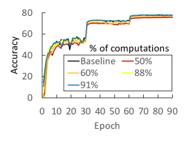
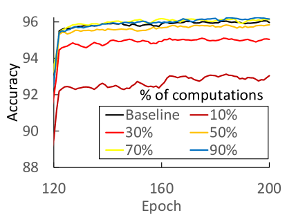
Refer to caption
Figure 10: Learning curves for WRN-28-10 CIFAR-10 validation accuracy under different top-k𝑘k sampling ratios. Focused view of last training epochs

D.4 ResNet-50 and ResNet-152 for ImageNet

The ImageNet [32] ILSVRC 2012 dataset contain 1.2 million training images of varying dimensions split into 1000 classes. The validation set includes 50K images and the test set consists of 100K images.

For ResNet-50 [31] we use the implementation in https://github.com/pytorch/examples/tree/master/imagenet, available under BSD 3-Clause License. See [31] for further details on ResNet-50 architecture.

Image preprocessing includes random 224x224 crop, horizontal flipping and image normalization. The optimizer is Momentum SGD with momentum=0.9 and 1e-4 weight decay. Learning rate is 0.1 and it is decayed by 10 every 30 epochs. We use batch size of 256, cross-entropy loss and train the model for 90 epochs.

We apply sampling to the convolutional layers except the first layer due to the small number of input channels (3) and the fully-connected layer.

Figure 11(a) shows the top-1 accuracy of ResNet-50 for different sampling ratios. The different data points correspond to 50% top-k𝑘k sampling applied to all the layers, all layers with at least 128 channels, 256 channels, 512 channels and 1024 channels.

Figure 11(b) shows the top-1 accuracy of ResNet-152 for different sampling ratios. The different data points correspond to 50% top-k𝑘k sampling applied to all the layers, all layers with at least 256 channels, 512 channels and 1024 channels.
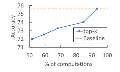
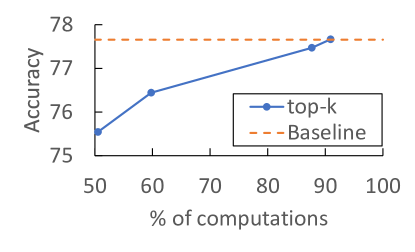
Refer to caption
(a) ResNet-50
Refer to caption
(b) ResNet-152
Figure 11: ResNet-50 and ResNet-152 ImageNet top-1 test accuracy. The accuracy increases as higher amounts of the computations are performed

Figures 6(b) and 6(c) show the top-1 validation accuracy learning curves for different forward-pass top-k𝑘k sampling ratios, compared to the non-approximate baseline. We observe that ResNet-50 and ResNet-152 are more sensitive to sampling compared to WRN-28-10 on CIFAR10. Nonetheless, applying 50% sampling in the layers with 1024 channels, corresponding to 93% of the computations in ResNet-50 and 91% of the computations in ResNet-152, follow the non-approximate learning curves almost identically.

D.5 Distributed Training

To evaluate the accuracy of top-k𝑘k-weights algorithm for ResNet-152 on Imagenet we used the same settings as in the previous section and trained on a single node with 4 GPUs. The accuracy results are shown in figure 12. The different data points correspond to 50% top-k𝑘k-weights sampling applied to all layers with at least 256 channels, 512 channels and 1024 channels.
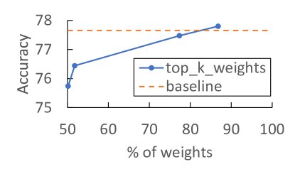
Refer to caption
Figure 12: ResNet-152 ImageNet top-1 test accuracy, using top-k𝑘k-weights algorithm.

For the distributed training experiments we used eight AWS EC2 instances equipped with 2.7GHz Intel Xeon E5-2686v4 CPU, one V100 GPU with 16 GB of memory, 10 Gbps networking, PyTorch version 1.7.1, CUDA 11 and Python 3.7.6.

For the distributed measurement we used the same hyper-parameters except the minibatch size which we set to 32 per GPU. We could not increase the batch size since the AWS EC2 GPU we used had 16GB of memory and could not support higher batch size. We note that the eight-node setting has a total global batch size of 256, which matches the batch size used in the accuracy evaluation.