Degree Distribution of Delaunay Triangulations

Abstract

Delaunay triangulation can be considered as a type of complex networks. For complex networks, the degree distribution is one of the most important inherent characteristics. In this paper, we first consider the two- and three-dimensional Delaunay Triangulations (DTs) as a type of complex networks, and term it as DT networks. Then we statistically investigate the degree distribution of DT networks. We find that the degree distribution of DT networks well follows the Gaussian distribution in most cases, which differs from the Poisson distribution and the Power-Law distribution for the well-known Small-World networks and Scale-Free networks.

1 Introduction

Quite recently, an exciting application of the Artificial Intelligence (AI) [1] is that: scientists have used Deep Learning algorithms [2] to recreate the complex neural codes that the place cells and grid cells in the brain use to navigate through space [3]. The grid cells discovered by May-Britt Moser and Edvard Moser [4] are capable of providing a strikingly periodic representation of self-location and navigation in the space [5], which spatially distributes as the hexagonal lattices. An interesting phenomenon is that: if considering each grid cell as a distinct point and then creating a triangulation for those scattered points, then a nice triangulation can be generated since each point has six neighboring points and triangles. In a triangulation (more precisely, a triangular mesh in this case), the quality of each triangle could be very high when each point has six neighboring points and triangles since the triangles could be close to the Regular Triangles. In other words, when each point in a triangulation has the degree of six, a very high-quality triangulation can be generated.

When using a triangulation to represent the spatial connection of the grid cells, a network (or so-called complex network) could be achieved. In the network of grid cells, the degree of each vertex is in general six. That is, the grid cell network represented with a triangulation is a 6-regular network with uniform degree distribution. However, for other complex networks such as the biological networks or the social networks, most of them are not regular networks but the so-called Small-World networks [6] or the Scale-Free networks [7]. The degree distributions of the Small-World networks and the Scale-Free networks are not uniform, but generally follow the Poisson distribution and the Power-Law distribution, respectively.

Inspired by representing the grid cells with triangulations, we consider a specific category of the triangulations, i.e., the Delaunay Triangulation (DT) [8], as a type of complex networks. We term this network as the DT network. More specifically, we consider the two-dimensional DT (i.e., the triangular mesh) and the three-dimensional DT (i.e., the tetrahedral mesh) as a specific type of complex networks; and we ignore those higher-dimensional DTs. Furthermore, we are quite interested in statistically investigating the degree distribution of the DT networks. To the best of the authors’ knowledge, there is no previous work specifically focusing on this problem.

Our work in this paper can be summarized as follows. First, we consider the two- and three-dimensional DTs as a specific type of complex networks that is termed as the DT network. Second, we statistically investigate the degree distribution of the DT network, and find that the degree distribution follows a Gaussian function, while in contrast the degree distributions of two well-known networks, i.e., the Small-World networks [6] and the Scale-Free networks [7] follow a Poisson function and a Power-Law function, respectively.

2 Method

2.1 Considering Delaunay Triangulations as A Type of Complex Networks

In mathematics, for a set P of points in the $d$-dimensional Euclidean space, a Delaunay Triangulation [8] is a triangulation DT(P) such that no point in $P$ is inside the circum-hypersphere of any d-simplex in DT(P). It is known [8] that there exists a unique Delaunay triangulation for P if P is a set of points in general position. For a set of two-dimensional points P, the DT(P) is a triangulation such that no point in P is inside the circumcircle of any triangle in DT(P). For a set of three-dimensional points P, the DT(P) is a triangulation such that no point in P is inside the circumscribing sphere of any tetrahedron in DT(P).

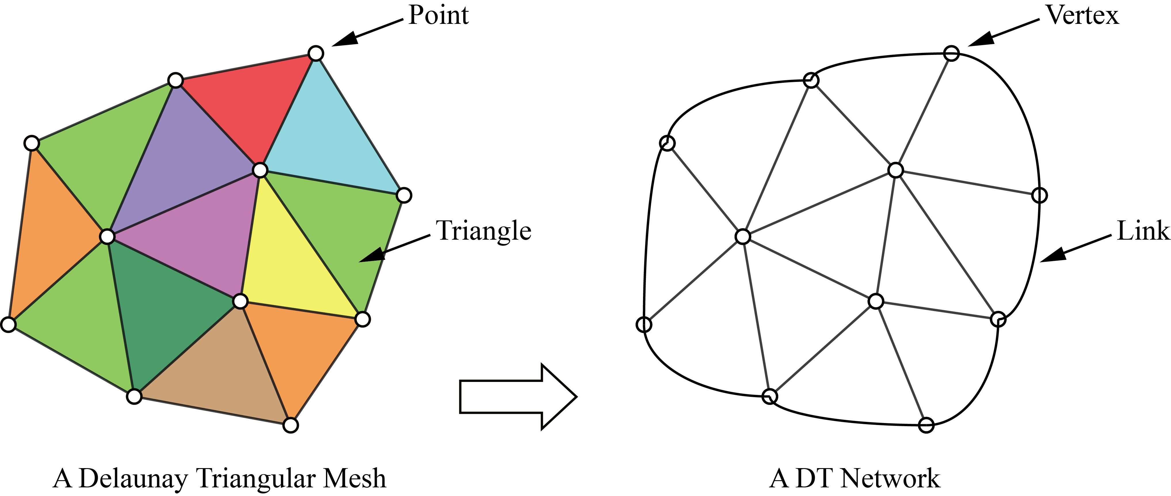
In the context of network theory, a complex network is a graph (network) with non-trivial topological features. In this paper, we consider the two- and three-dimensional DTs [8], i.e., the Delaunay triangular meshes and the Delaunay tetrahedral meshes, as a specific type of complex networks. More precisely, we consider that: each vertex in a DT represents a cell, a person, or even a device in a complex network, while each edge in a DT represents the link or connection between vertices; see Figure 1.

Figure 1: Consideration of a DT as a complex network

2.2 Investigating the Degree Distribution of DT Networks

In this paper, we are interested in statistically investigating the degree distribution of two- and three-dimensional DT networks. The DT networks are in fact the Delaunay triangular meshes in two-dimensions and the Delaunay tetrahedral meshes in three-dimensions. To statistically examine the degree distribution of DT networks, we first create five groups of triangular meshes and tetrahedral meshes based on sets of scattered points. Each set of scattered points are randomly generated, and then are used to create the triangular or tetrahedral meshes using the two famous Delaunay mesh generators, Triangle [9] or TetGen [10].

For each DT network, we first obtain the vertex degree (i.e., the number of neighboring vertices) for each vertex, and then count the degrees of all vertices to obtain the discrete frequency of vertex degree. The frequency of vertex degree is represented in percentage. Finally, the frequency of vertex degree is fitted to a Gaussian function (Eq.(1)):

$$y=ae^{-\frac{(x-b)^{2}}{2c^{2}}}+y_{0},$$ (1)

where, the parameters $a$, $b$, $c,$ and $y_{0}$ are arbitrary real numbers.. The graph of a Gaussian is a characteristic ”bell curve” shape. The parameter $a$ is the height of the curve’s peak; $b$ (the mean) is the position of the center of the peak; $c$ (the standard deviation) controls the width of the ”bell”; and $y_{0}$ is the offset.

After fitted the frequency of vertex degrees to the Gaussian model, we use the R-Square (R${}^{2})$ and Adjusted R-Square (Adj. R${}^{2})$ to evaluate the Goodness of Fit.

3 Results and Discussion

3.1 Degree Distribution of Two-dimensional DT Networks

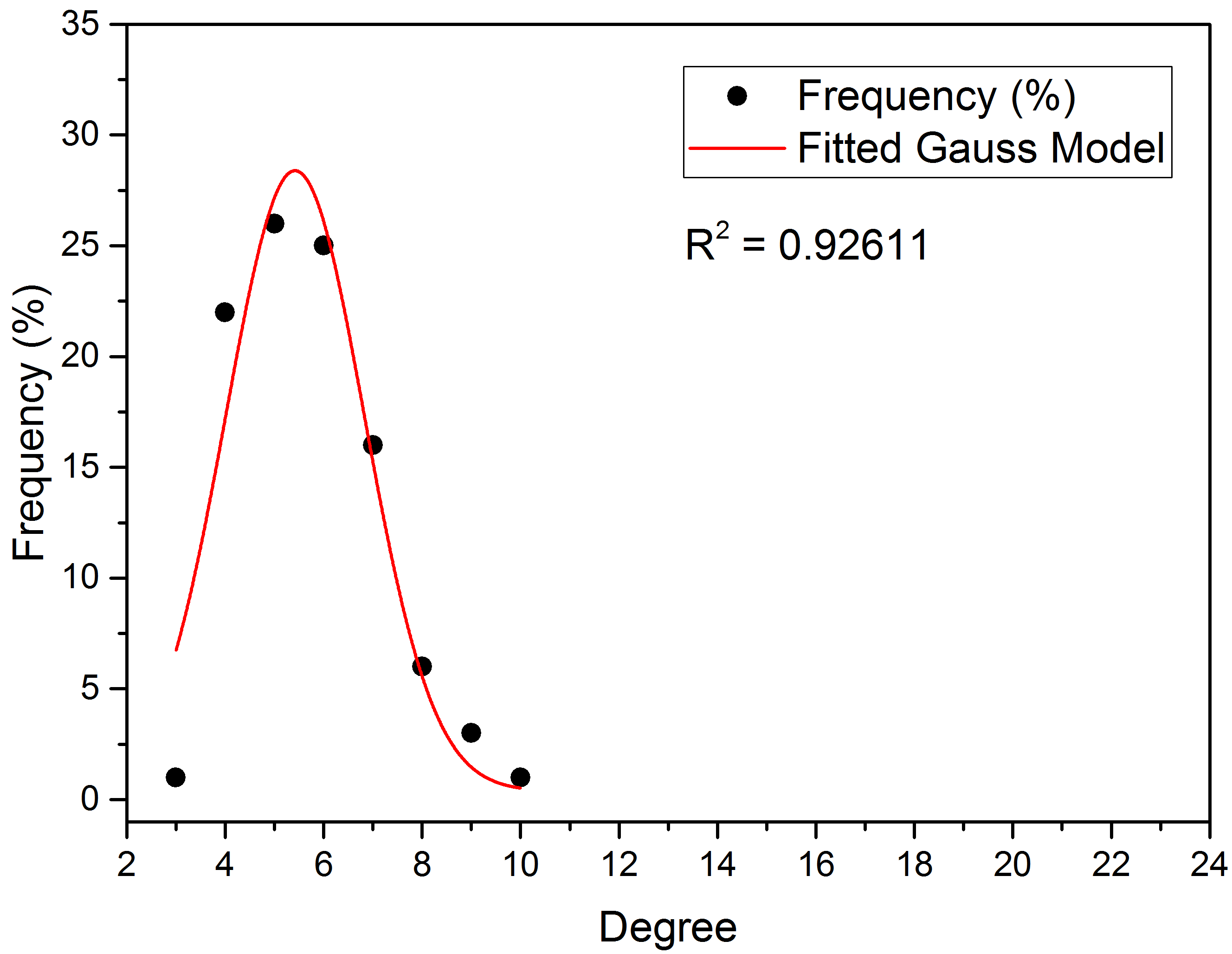
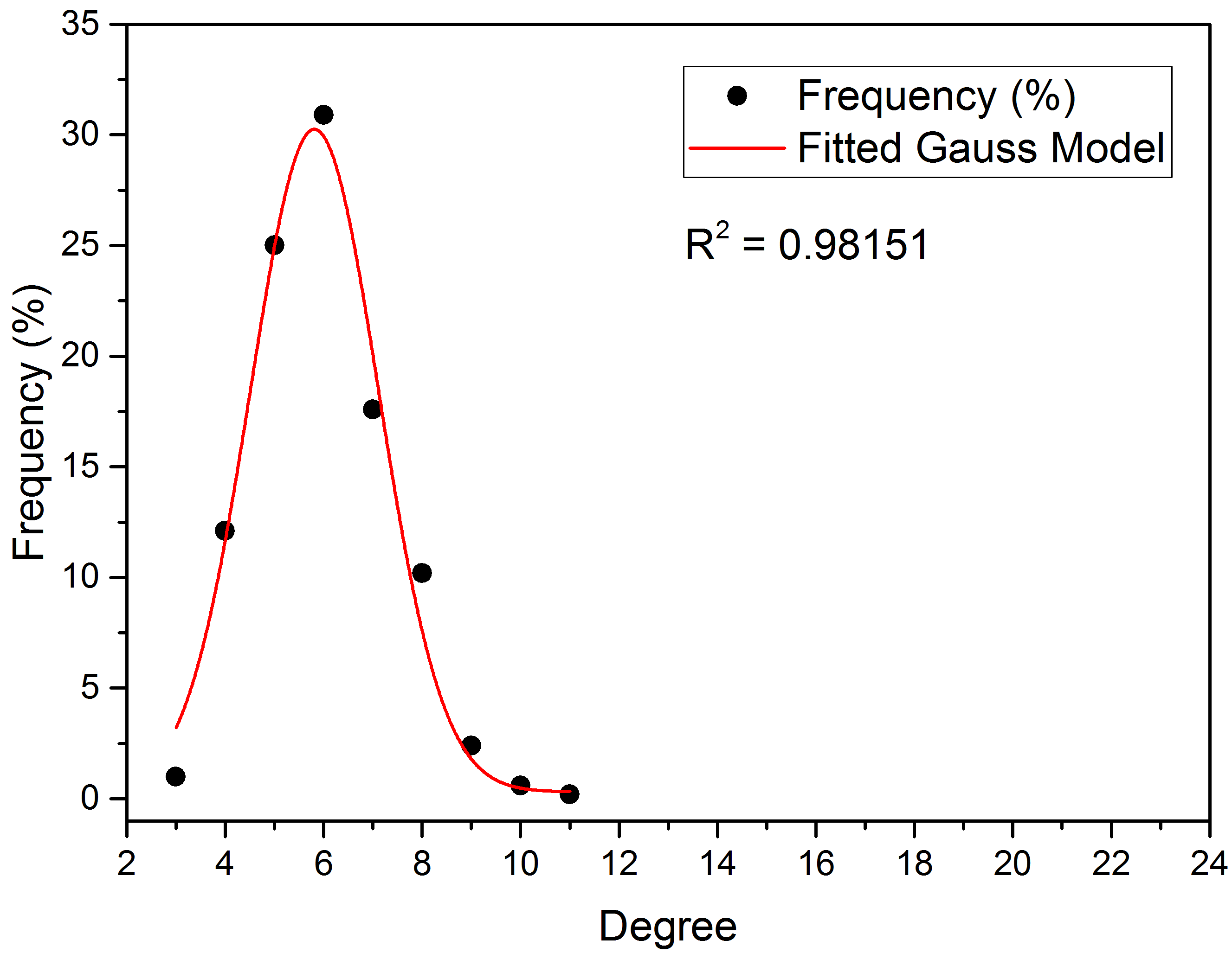
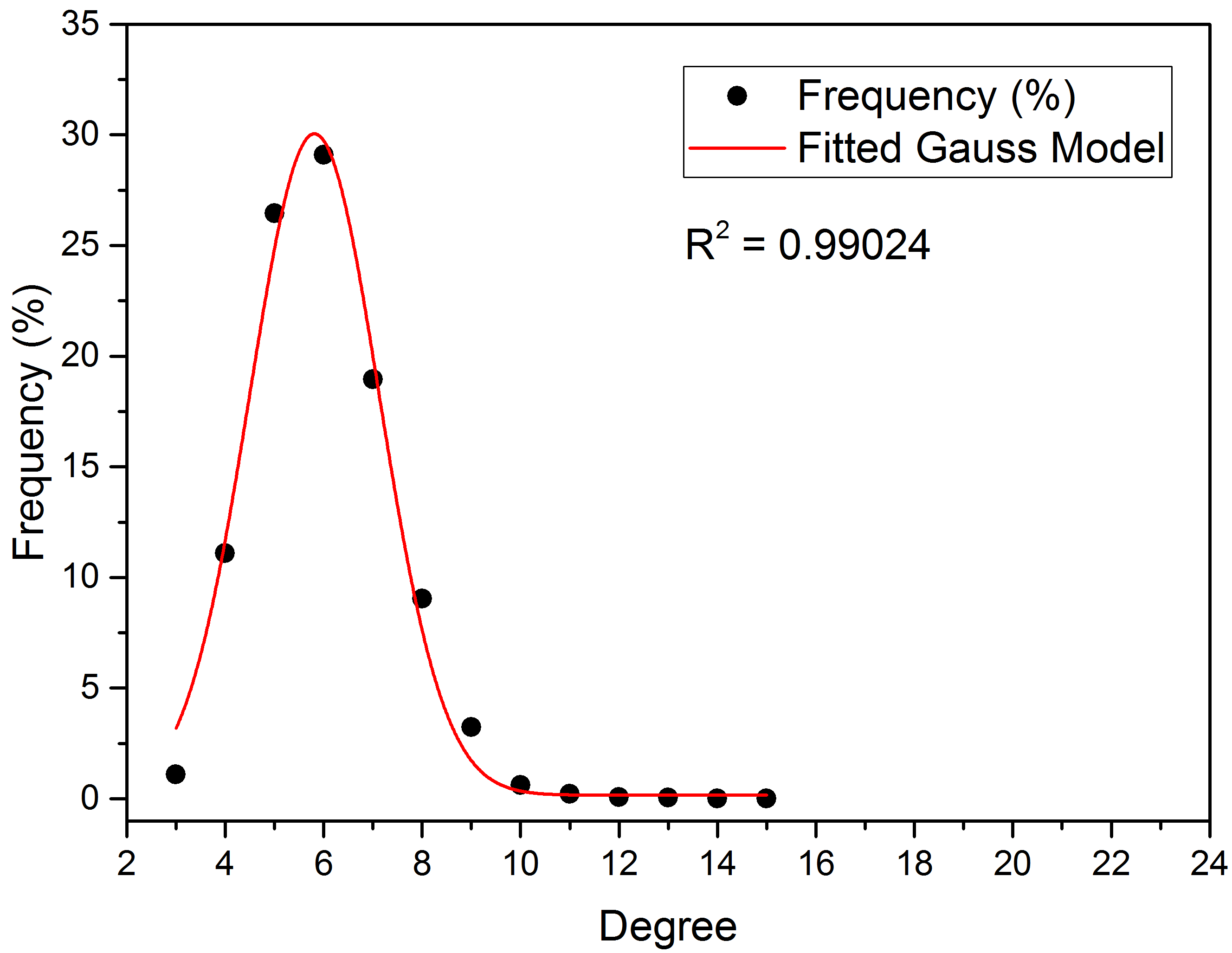
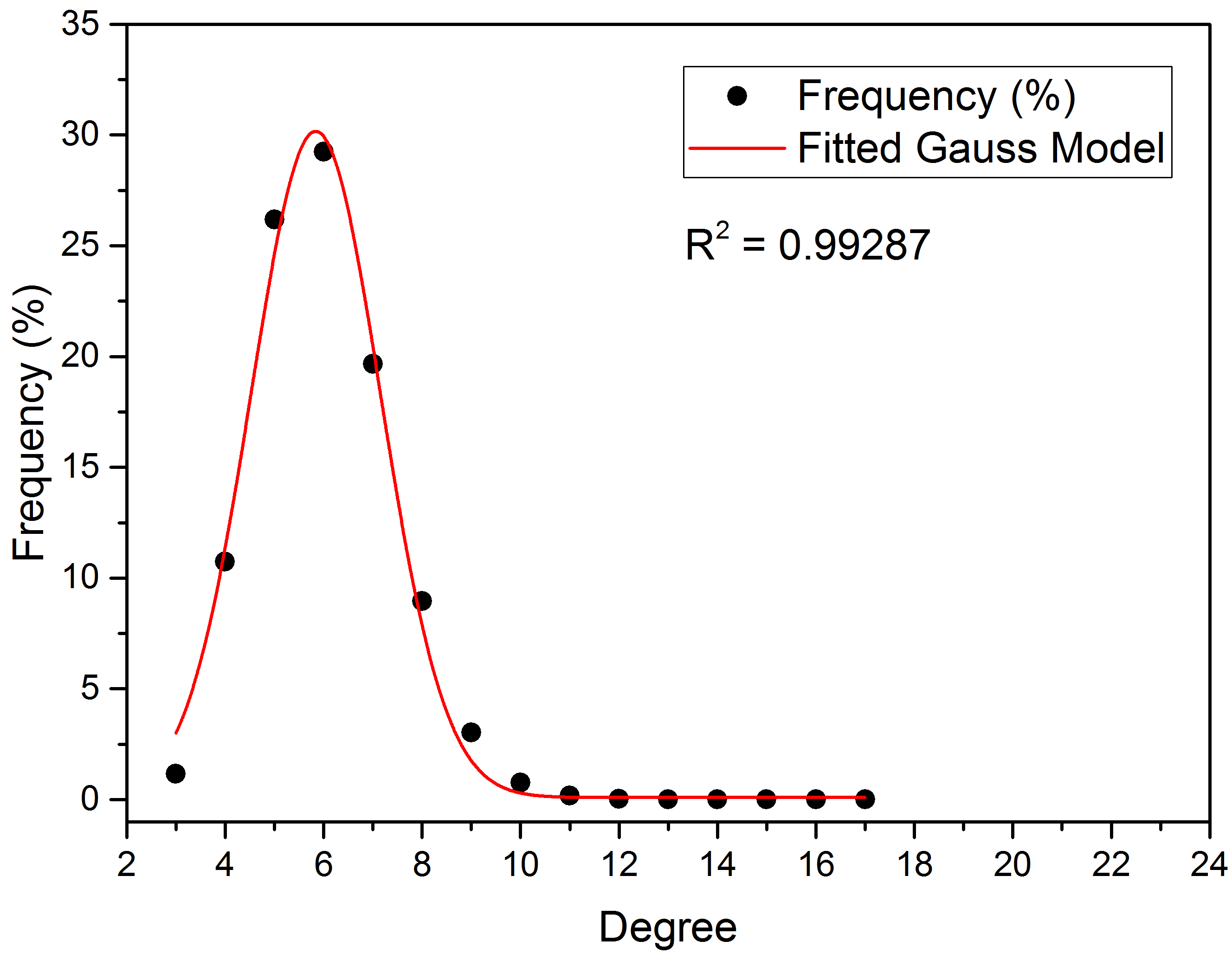
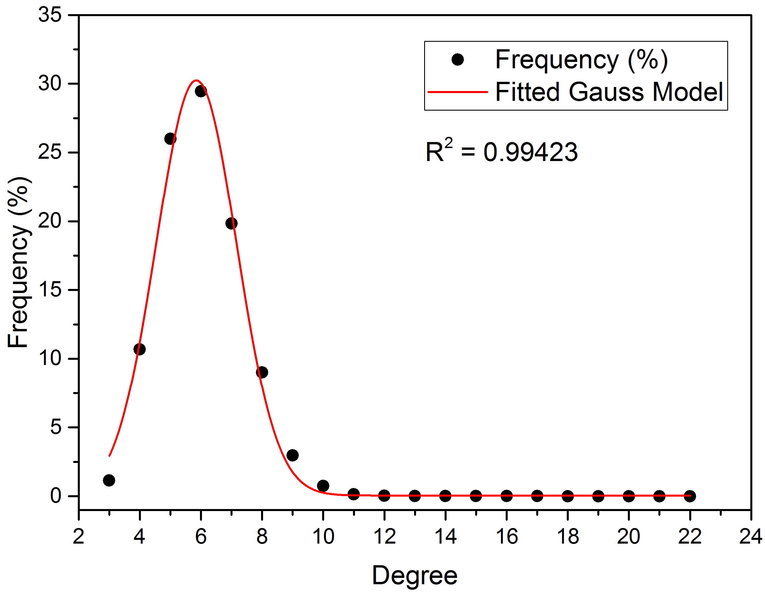
We first determine five different sizes of sets of scattered points (i.e., 100, 1000, 10000, 100000, and 1000000). For each size, we repeatedly create five two-dimensional Delaunay triangulations. And there are totally 25 Delaunay triangular meshes. For all of the 25 meshes, we calculate the vertex degrees, count the frequency of vertex degree, and fit the frequency of vertex degree to the Gaussian Model (Eq. (1)). We employ the R-Square (R${}^{2})$ and Adjusted R-Square (Adj. R${}^{2})$ to measure the Goodness of fit. Details of the fitted Gaussian Models are listed in Table 1. For each size, we also plot one of the fitted Gaussian Models (see Figure 2).

The results presented in Table 1 and Figure 2 indicate that:

1. the degree distribution of two-dimensional DT network well follows the Gaussian Distribution in most cases;

2. with the increase of the number of vertices in DT networks, the fitting of the frequency of vertex degree to a Gaussian model becomes better.

(a) A DT network with 100 vertices

(b) A DT network with 1000 vertices

(c) A DT network with 10,000 vertices

(d) A DT network with 100,000 vertices

(e) A DT network with 1,000,000 vertices

Figure 2: Fitted Gaussian models for five different sizes of two-dimensional DT networks

(a) A DT network with 100 vertices

(b) A DT network with 1000 vertices

(c) A DT network with 10,000 vertices

(d) A DT network with 100,000 vertices

(e) A DT network with 1,000,000 vertices

Figure 3: Fitted Gaussian models for five different sizes of three-dimensional DT networks

3.2 Degree Distribution of Three-dimensional DT Networks

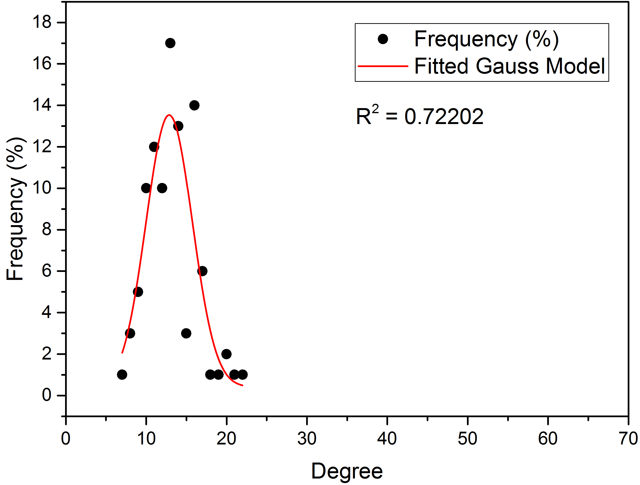
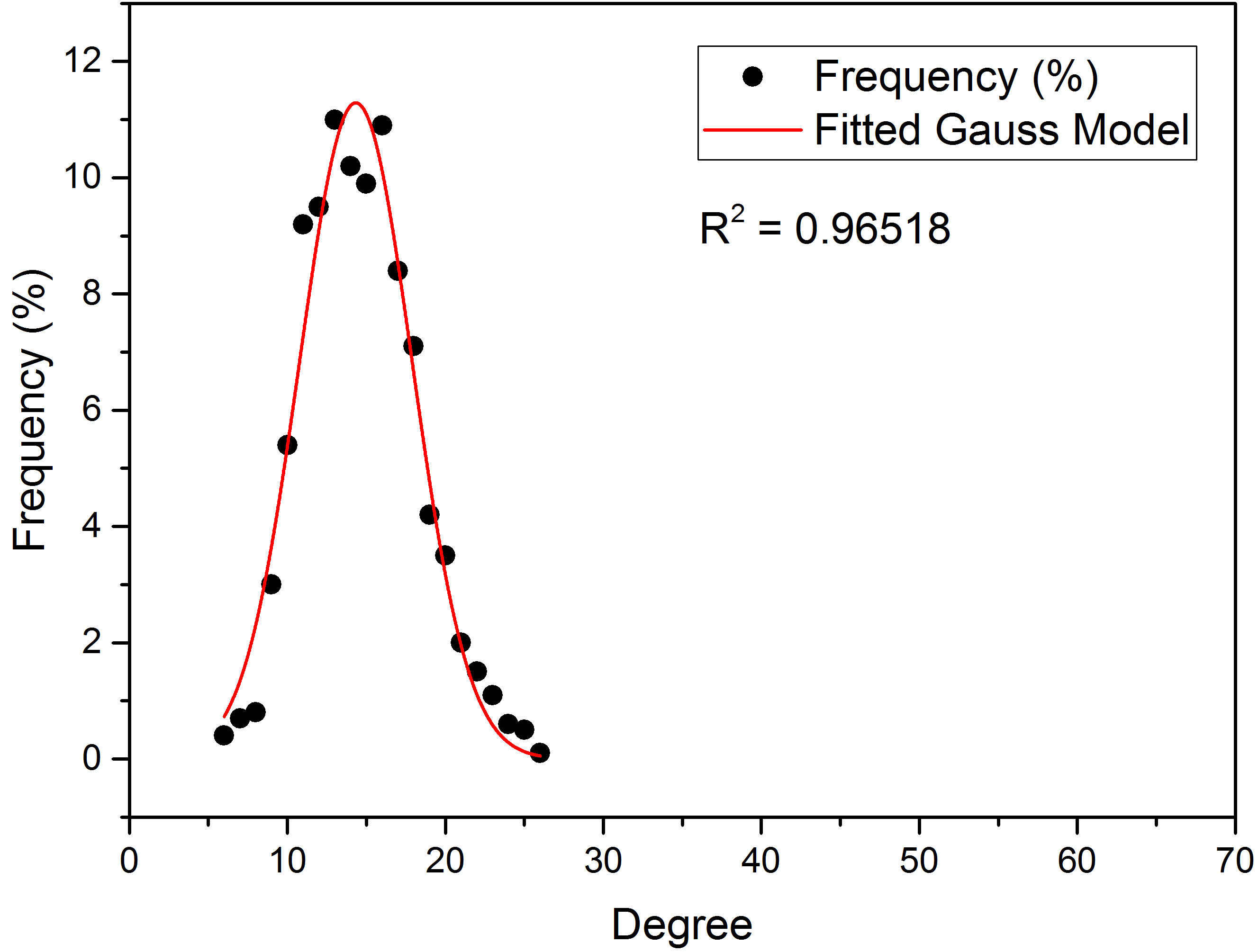
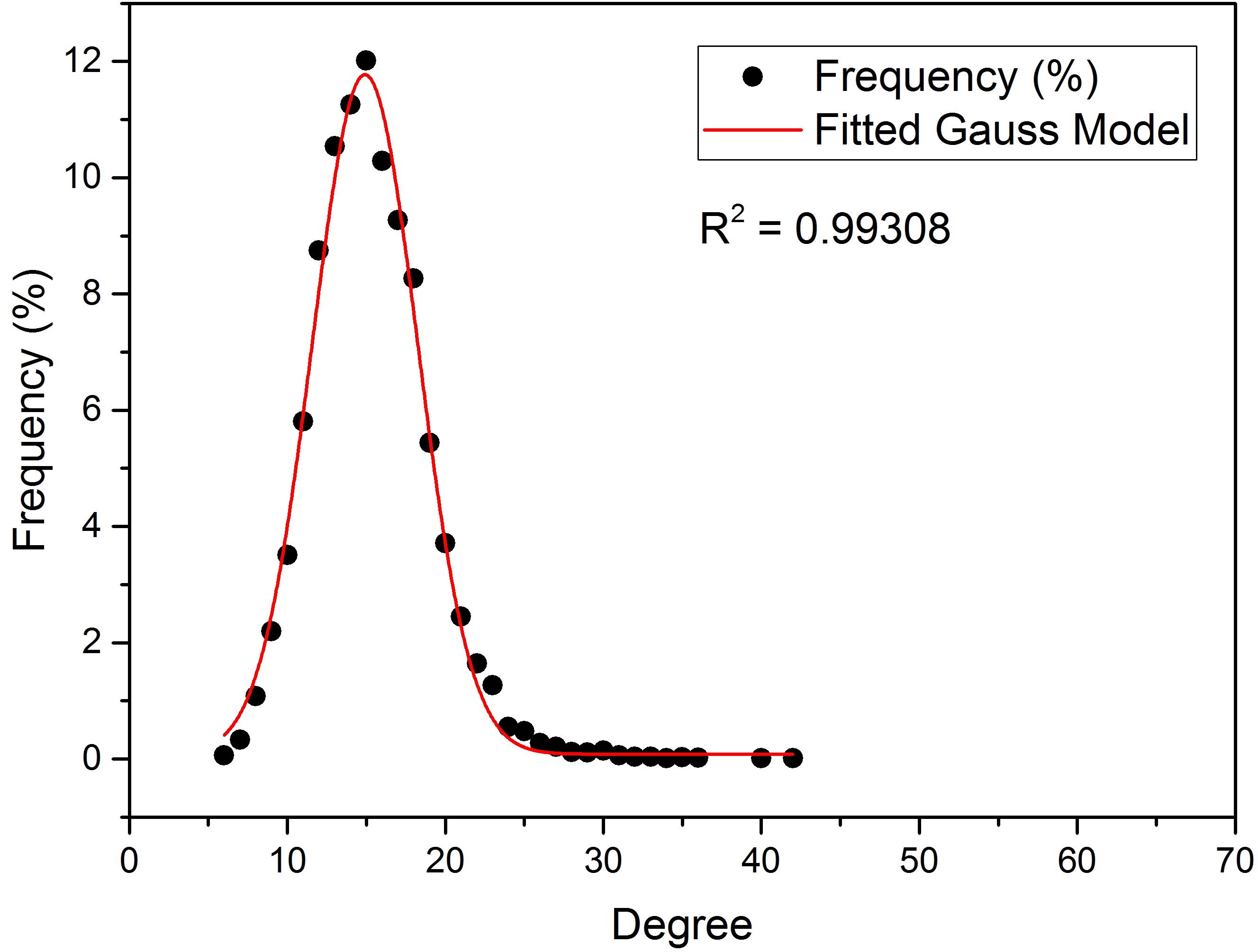
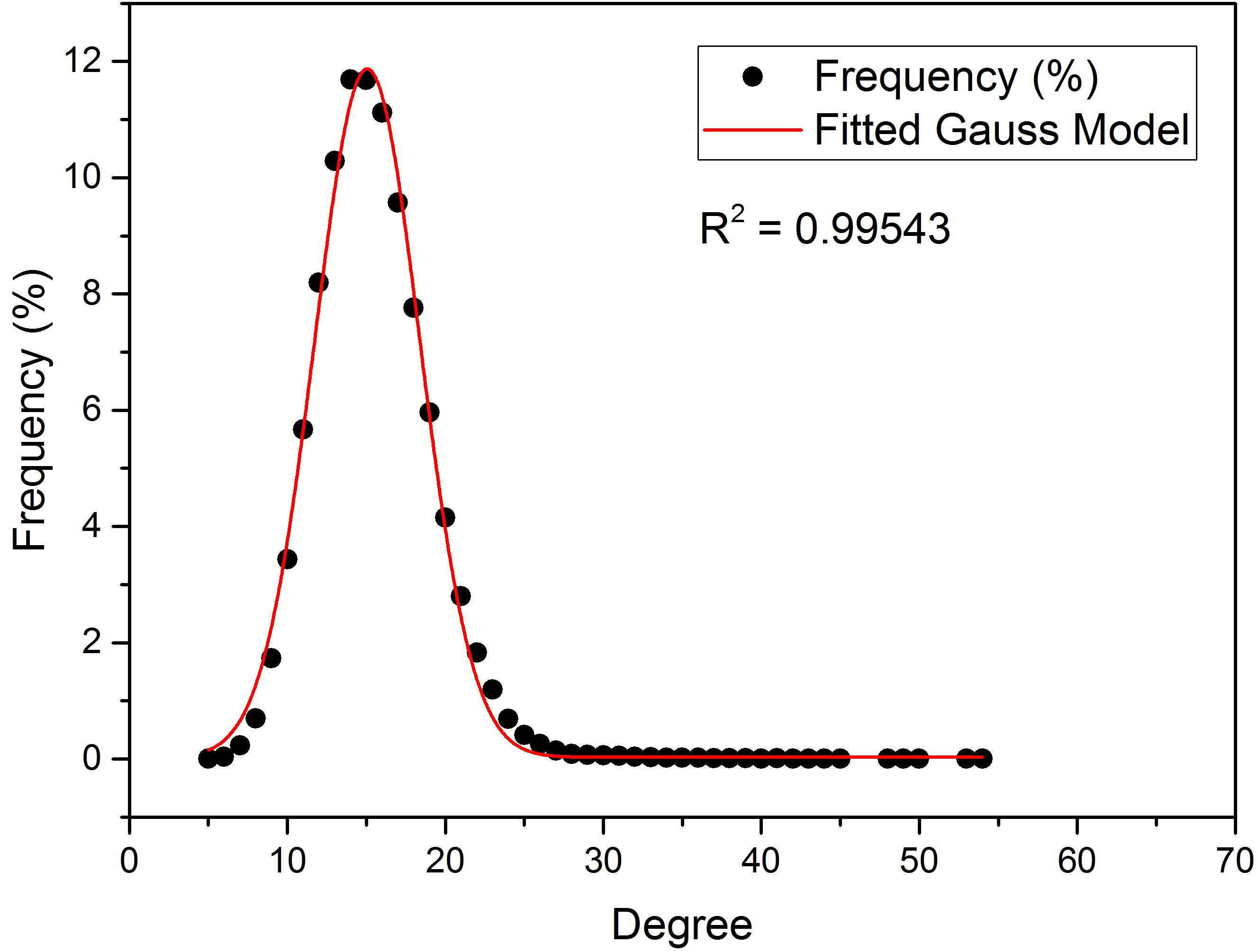
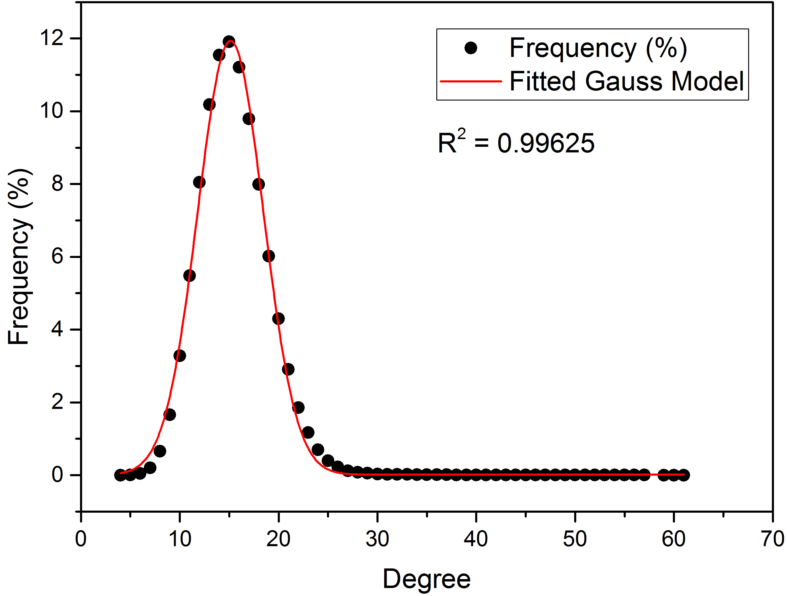
As the same as the investigation of the degree distribution of two-dimensional DT networks, for the three-dimensional ones, we also determine five different sizes of sets of scattered points. For each size, we repeatedly create the Delaunay tetrahedral meshes five times. We calculate the frequency of vertex degree, and then fit the frequency of vertex degree to the Gaussian function (Eq. (1)). Details of the fitted Gaussian Models are listed in Table 2. For each size, we also plot one of the fitted Gaussian Models (see Figure 3).

The results presented in Table 2 and Figure 3 indicate that:

1. the degree distribution of three-dimensional DT networks also well follows the Gaussian Distribution except for the very small size of DTs (see Figure 3(a));

2. with the increase of the number of vertices in DT networks, the frequency of vertex degree becomes more and more fitted to a Gaussian function. This is the same as that for the two-dimensional DT networks.

Table 1: Details of the fitted Gaussian models for five different sizes of two-dimensional DT networks

Num. of Vertices	Parameters of the Fitted Gauss Model				Goodness of Fit		Figure
	a	b	c	y0	R2	Adj. R2
102	28.00545	5.41927	1.40459	0.38407	0.92611	0.87069	Figure 2(a)
	29.68097	5.44527	1.27589	0.74051	0.93000	0.87750
	34.52490	5.98086	0.87684	4.03527	0.96943	0.92357
	34.08906	5.50212	0.98915	1.94301	0.97739	0.96043
	25.83382	5.41456	1.34654	1.75594	0.99149	0.98510
103	29.93515	5.81252	1.30081	0.31490	0.98151	0.97041	Figure 2(b)
	29.93834	5.72799	1.20473	0.98548	0.98386	0.97579
	29.76963	5.76064	1.27671	0.51488	0.98669	0.98004
	29.16937	5.80171	1.35679	0.15905	0.98987	0.98379
	29.90300	5.84234	1.29982	0.29798	0.99680	0.99519
104	29.88082	5.81242	1.31279	0.16539	0.99024	0.98699	Figure 2(c)
	29.93680	5.82429	1.30700	0.19757	0.99281	0.99011
	30.25405	5.82634	1.29838	0.11202	0.99342	0.99145
	30.38152	5.83662	1.28568	0.22451	0.99420	0.99172
	29.89607	5.84881	1.31856	0.12675	0.99494	0.99326
105	30.06407	5.83894	1.31350	0.09805	0.99287	0.99093	Figure 2(d)
	30.16499	5.84439	1.30954	0.09481	0.99375	0.99205
	30.19954	5.84569	1.30756	0.09675	0.99415	0.99255
	30.07007	5.84758	1.31579	0.07981	0.99420	0.99275
	30.13382	5.84836	1.31393	0.07511	0.99428	0.99285
106	30.18968	5.84948	1.31402	0.05053	0.99423	0.99315	Figure 2(e)
	30.08914	5.84862	1.31909	0.04873	0.99424	0.99316
	30.18773	5.85070	1.31355	0.05832	0.99427	0.99305
	30.21144	5.84841	1.31170	0.05835	0.99427	0.99313
	30.23149	5.84921	1.31112	0.05422	0.99432	0.99326

Table 2: Details of the fitted Gaussian models for five different sizes of three-dimensional DT networks

Num. of Vertices	Parameters of the Fitted Gauss Model				Goodness of Fit		Figure
	a	b	c	y0	R2	Adj. R2
102	13.12919	12.86086	2.88146	0.40405	0.72202	0.65253	Figure 3(a)
	14.08050	11.59738	1.88705	2.22933	0.79719	0.74188
	13.46764	12.53566	2.87983	0.52913	0.82998	0.77331
	13.12995	12.38275	2.85504	0.46392	0.83969	0.79597
	11.77248	11.92589	3.00907	1.35579	0.91722	0.89239
103	11.28722	14.33136	3.55809	0.00020	0.96518	0.95904	Figure 3(b)
	11.64593	14.11783	3.05218	0.46269	0.96882	0.96414
	12.10603	14.39760	3.14854	0.19478	0.97574	0.97210
	11.34799	14.36068	3.42533	0.13816	0.97641	0.97248
	11.16427	14.30988	3.36066	0.28659	0.98464	0.98234
104	11.68965	14.90960	3.32630	0.08346	0.99308	0.99236	Figure 3(c)
	11.56788	14.88169	3.39803	0.05132	0.99342	0.99276
	11.47522	14.86408	3.42240	0.04812	0.99346	0.99287
	11.69194	14.83496	3.31919	0.08442	0.99356	0.99293
	11.63035	14.79683	3.32669	0.09591	0.99378	0.99316
105	11.84302	15.05391	3.32420	0.03019	0.99543	0.99510	Figure 3(d)
	11.83560	15.05495	3.32932	0.02664	0.99577	0.99547
	11.86178	15.06382	3.32584	0.02517	0.99583	0.99554
	11.85270	15.05600	3.32674	0.02680	0.99602	0.99574
	11.86734	15.05052	3.31587	0.03080	0.99603	0.99574
106	11.92144	15.13136	3.32073	0.01385	0.99625	0.99604	Figure 3(e)
	11.93135	15.13290	3.31960	0.01300	0.99628	0.99607
	11.92786	15.13621	3.31965	0.01348	0.99638	0.99617
	11.92595	15.13733	3.31972	0.01397	0.99639	0.99619
	11.92224	15.13856	3.32184	0.01250	0.99647	0.99628

4 Conclusion

In this paper, we first considered the two- and three-dimensional DTs as a type of complex networks, i.e., the DT network; and then we investigated the degree distribution of the DT networks. It has been found that the degree distribution of the DT networks well follows the Gaussian distribution in most cases. This is different from the Power-Law degree distributions in the Scale-Free networks and the Poisson degree distribution in the Small-World networks.

In real-world applications, perhaps there are few complex systems can be exactly represented by the DT network. However, it is possible that in some cases scientists may try to use the DT network to approximately represent the quite complex biological network in the brain, and reveal the structural correlations of the biological networks [11, 12, 13].

References

- [1] Savelli, F. and J.J. Knierim, AI mimics brain codes for navigation. Nature, 2018. 557(7705): p. 313-314.
- [2] LeCun, Y., Y. Bengio, and G. Hinton, Deep learning. Nature, 2015. 521: p. 436.
- [3] Banino, A., et al., Vector-based navigation using grid-like representations in artificial agents. Nature, 2018.
- [4] Hafting, T., et al., Microstructure of a spatial map in the entorhinal cortex. Nature, 2005. 436: p. 801.
- [5] Doeller, C.F., C. Barry, and N. Burgess, Evidence for grid cells in a human memory network. Nature, 2010. 463: p. 657.
- [6] Watts, D.J. and S.H. Strogatz, Collective dynamics of ’small-world’ networks. Nature, 1998. 393(6684): p. 440-442.
- [7] Barabasi, A.L. and R. Albert, Emergence of scaling in random networks. Science, 1999. 286(5439): p. 509-512.
- [8] Delaunay, B., Sur la sphère vide. Bulletin de l’Académie des Sciences de l’URSS, Classe des sciences mathématiques et naturelles, 1934. 6: p. 793–800.
- [9] Shewchuk, J.R., Delaunay refinement algorithms for triangular mesh generation. Computational Geometry-Theory and Applications, 2002. 22(1-3): p. 21-74.
- [10] Si, H., TetGen, a Delaunay-Based Quality Tetrahedral Mesh Generator. Acm Transactions on Mathematical Software, 2015. 41(2).
- [11] Rubinov, M. and O. Sporns, Complex network measures of brain connectivity: Uses and interpretations. NeuroImage, 2010. 52(3): p. 1059-1069.
- [12] Bullmore, E. and O. Sporns, Complex brain networks: graph theoretical analysis of structural and functional systems. Nature Reviews Neuroscience, 2009. 10: p. 186.
- [13] Avena-Koenigsberger, A., B. Misic, and O. Sporns, Communication dynamics in complex brain networks. Nature Reviews Neuroscience, 2018. 19(1): p. 17-33.