NEWMA: a new method for scalable model-free online change-point detection

Nicolas Keriven CNRS, GIPSA-lab. Damien Garreau Université Côte d’Azur, Inria, CNRS, LJAD. Iacopo Poli LightOn.
Abstract

We consider the problem of detecting abrupt changes in the distribution of a multi-dimensional time series, with limited computing power and memory. In this paper, we propose a new, simple method for model-free online change-point detection that relies only on fast and light recursive statistics, inspired by the classical Exponential Weighted Moving Average algorithm (EWMA). The proposed idea is to compute two EWMA statistics on the stream of data with different forgetting factors, and to compare them. By doing so, we show that we implicitly compare recent samples with older ones, without the need to explicitly store them. Additionally, we leverage Random Features (RFs) to efficiently use the Maximum Mean Discrepancy as a distance between distributions, furthermore exploiting recent optical hardware to compute high-dimensional RFs in near constant time. We show that our method is significantly faster than usual non-parametric methods for a given accuracy.

1 Introduction

The goal of online change-point detection is to detect abrupt changes in the distribution of samples in a data stream. One seeks to detect a change as soon as it occurs, while minimizing the number of false alarms. Online change-point detection has numerous practical applications, for instance medical monitoring via the segmentation of EEG, ECG and fMRI signals [33, 41, 7], or detections of changes in audio [6] or video [28, 1] streams. We refer to [35] for a thorough review. In recent applications, the need arises to perform such methods on embedded devices, for instance in video streams from body-worn or surveillance video cameras [2], or on data collected by smart phones [27]. In addition to being constrained by limited power and memory, such personal devices collect data that can be potentially sensitive, hence the need to process the stream on-the-fly, ideally without storing any raw data.

In this paper, we propose a new approach for online, non-parametric change-point detection, whose main advantage is that it does not require to store any raw data in memory, but only appropriate smoothed quantities. It is inspired by: a) the classical Exponentially-Weighted Moving Average (EWMA), but requires less prior knowledge about the in-control distribution of the data, and b) a simple Sliding Window (SW) strategy in its model-free version, but is more efficient in memory and preserves data privacy.

1.1 Framework: model-free methods and generalized moments

We consider a stream of samples (xt)tsubscriptsubscript𝑥𝑡𝑡\left(x_{t}\right)_{t\in\mathbb{N}} with values in dsuperscript𝑑\mathbb{R}^{d} with potentially large d𝑑d. The goal of online change-point detection is to detect changes in the distribution of the samples xtsubscript𝑥𝑡x_{t} in a sequential manner. We assume that the samples are independent and identically distributed (i.i.d.formulae-sequence𝑖𝑖𝑑i.i.d.) before and after each change, and that there may be multiple changes in a row to be detected on-the-fly. As we will see, some methods assume prior knowledge about the distributions before (and sometimes after) each change, however we will consider that no prior knowledge is available here, and develop a so-called model-free method.

Historically, many methods assume that the distributions of interest belong to a parametric family of distributions whose likelihood pθsubscript𝑝𝜃p_{\theta} is entirely specified (often Gaussians), and rely on a (generalized) likelihood ratio (GLR) test. However, such a complete specification is not always available. In a non-parametric context, some methods then rely on approximating generic discrepancies between distributions such as the Kullback-Leibler (KL) divergence, the total variation [3] or some optimal transport-based distances [9]. However, it is well-known [44] that most of these metrics are difficult to estimate in high dimension d𝑑d, and/or may be too costly to compute in an online framework. On the contrary, simpler methods are designed to detect changes in some quantity related to the distribution such as the mean or the variance [13]. We consider a generalization of this last concept, namely, to detect changes in a collection of generalized moments θΨ(π)=def.𝔼xπΨ(x)superscriptdef.subscript𝜃Ψ𝜋subscript𝔼similar-to𝑥𝜋Ψ𝑥\theta_{\Psi}(\pi)\stackrel{{\scriptstyle\textrm{{def.}}}}{{=}}\mathbb{E}_{x\sim\pi}\Psi\left(x\right), where π𝜋\pi is the distribution of the samples, and Ψ:d:Ψsuperscript𝑑\Psi:\mathbb{R}^{d}\to\mathcal{H} is a mapping to a normed space (,)(\mathcal{H},\left\|\cdot\right\|) (generally, =msuperscript𝑚\mathcal{H}=\mathbb{R}^{m} or msuperscript𝑚\mathbb{C}^{m}). We therefore introduce the following pseudometric on distributions:

dΨ(π,π)=def.𝔼πΨ(x)𝔼πΨ(x),superscriptdef.subscript𝑑Ψ𝜋superscript𝜋normsubscript𝔼𝜋Ψ𝑥subscript𝔼superscript𝜋Ψ𝑥d_{\Psi}(\pi,\pi^{\prime})\stackrel{{\scriptstyle\textrm{{def.}}}}{{=}}\left\|\mathbb{E}_{\pi}\Psi\left(x\right)-\mathbb{E}_{\pi^{\prime}}\Psi\left(x\right)\right\|\,, (1)

which measures how different two distributions are in terms of these moments. For instance, when Ψ=IdΨId\Psi=\textrm{{Id}}, then θΨ(π)=𝔼xsubscript𝜃Ψ𝜋𝔼𝑥\theta_{\Psi}(\pi)=\mathbb{E}x, and the underlying assumption is that changes will occur in the mean of the distribution of the samples. This also includes higher order moments (Ψ(x)=xkΨ𝑥superscript𝑥tensor-productabsent𝑘\Psi(x)=x^{\otimes k}) or histograms (Ψ(x)=(1xBi)i=1kΨ𝑥superscriptsubscriptsubscript1𝑥subscript𝐵𝑖𝑖1𝑘\Psi(x)=(1_{x\in B_{i}})_{i=1}^{k} where the Bisubscript𝐵𝑖B_{i} are regions of space). If infinite-dimensional spaces \mathcal{H} such as Reproducing Kernel Hilbert Spaces (RKHS) are considered, this framework also includes the so-called kernel change-point detection [25, 19], and dΨsubscript𝑑Ψd_{\Psi} is then referred to as the Maximum Mean Discrepancy (MMD) [22]. We note that this framework does not, strictly speaking, include centered moments such as the variance, however one could modify the definition of dΨsubscript𝑑Ψd_{\Psi} to compute the variance from first order and second-order moments. We do not consider centered moments here for simplicity.

If the user has prior knowledge about which quantity θΨ(π)subscript𝜃Ψ𝜋\theta_{\Psi}(\pi) is susceptible to change over time, then ΨΨ\Psi can be chosen accordingly. If not, we will see in Sec. 4 that a somewhat “universal” embedding can be obtained by taking ΨΨ\Psi as kernel random features [36], which allows to efficiently approximate the MMD with high probability and controlled memory resources.

1.2 Prior knowledge on the in-control statistic

As mentioned above, some methods assume prior knowledge about the in-control distribution, that is, the distribution before the change. In our framework, it corresponds to the knowledge of the generalized moments θ=θΨ(π)superscript𝜃subscript𝜃Ψsuperscript𝜋\theta^{\star}=\theta_{\Psi}(\pi^{\star}), where πsuperscript𝜋\pi^{\star} is the in-control distribution.

One such classical approach is the Exponential Weighted Moving Average (EWMA) algorithm [37], which we describe111Note that our description of EWMA is similar to the original [37], with the addition that the data are transformed by the mapping ΨΨ\Psi. in Alg. 1. EWMA computes recursively a weighted average of Ψ(xt)Ψsubscript𝑥𝑡\Psi\left(x_{t}\right), with exponential weights that favor the more recent samples:

𝐳t=(1Λ)𝐳t1+ΛΨ(xt)subscript𝐳𝑡1Λsubscript𝐳𝑡1ΛΨsubscript𝑥𝑡\mathbf{z}_{t}=(1-\Lambda)\mathbf{z}_{t-1}+\Lambda\Psi\left(x_{t}\right)

where 0<Λ<10Λ10<\Lambda<1. When this average deviates too much from θsuperscript𝜃\theta^{\star}, an alarm is raised. The exponential weights (instead of, say, uniform weights) reduce the detection delay, and increase robustness to potentially irrelevant data in the past.

When =msuperscript𝑚\mathcal{H}=\mathbb{R}^{m}, a classical multivariate extension of EWMA is called Multivariate-EWMA, and rely on the fact that every dimension may not need the same forgetting factor, and therefore replace ΛΛ\Lambda by a diagonal matrix diag(Λ1,,Λm)diagsubscriptΛ1subscriptΛ𝑚\textrm{diag}\left(\Lambda_{1},\ldots,\Lambda_{m}\right). In our case there is no assumption on the marginals of the distribution of the data, and moreover it is not clear how the presence of the mapping ΨΨ\Psi would affect this strategy, hence we consider a single forgetting factor instead, and note however that our method could be extended when ΛΛ\Lambda is a matrix, which we leave for future work.

From our point of view, when considering high-dimensional data, the main advantage of EWMA is that it is extremely fast and have low memory footprint, due to its recursive nature: when a new sample arrives, the cost of the update is essentially that of computing Ψ(x)Ψ𝑥\Psi\left(x\right) once. Moreover, it preserves data privacy, in the sense that it never stores raw samples but only a smoothed statistic computed from them. However, EWMA requires the prior knowledge of θsuperscript𝜃\theta^{\star}, which severely limits its use in some cases where it is not available.

Stream of data xtsubscript𝑥𝑡x_{t}, function ΨΨ\Psi, in-control value θsuperscript𝜃\theta^{\star}, forgetting factor 0<Λ<10Λ10<\Lambda<1, threshold τ>0𝜏0\tau>0, initial value 𝐳0subscript𝐳0\mathbf{z}_{0}
for t=1,2,𝑡12t=1,2,\ldots do
   𝐳t=(1Λ)𝐳t1+ΛΨ(xt)subscript𝐳𝑡1Λsubscript𝐳𝑡1ΛΨsubscript𝑥𝑡\mathbf{z}_{t}=(1-\Lambda)\mathbf{z}_{t-1}+\Lambda\Psi\left(x_{t}\right)
   if 𝐳tθτnormsubscript𝐳𝑡superscript𝜃𝜏\left\|\mathbf{z}_{t}-\theta^{\star}\right\|\geq\tau then
      Flag t𝑡t as a change-point    
Figure 1: EWMA [37]

1.3 Methods without prior knowledge

To solve this last problem, methods with no prior knowledge requirement about the in-control distribution were proposed. Many of them are two-steps adaptation of the previous class of approaches: the parameter θsuperscript𝜃\theta^{\star} is estimated from some training samples during a Phase I, before the actual detection during a Phase II [26, 47]. In the online setting, where several changes can happen during a continuous run, this strategy is often adapted in a “sliding windows” approach: a window of recent samples is compared against a window of samples that came immediately before [3, 31, 30]. In our settings, given a window size B𝐵B, the most natural approach is to compare an empirical average of Ψ(x)Ψ𝑥\Psi\left(x\right) over the last B𝐵B samples with one computed on the B𝐵B samples that came before, to approximate dΨsubscript𝑑Ψd_{\Psi}. When the difference is higher than a threshold, an alarm is raised. We refer to this simple algorithm as Sliding Window222While this simple algorithm appears several times in the literature [3, 30], as far as we know it does not have a designated name. (SW, Alg. 2).

Such model-free methods are useful in a wide class of problems, since they can adapt to potentially any in-control situation. Despite these advantages, they can have a high memory footprint, since they store raw data that may be high-dimensional (see Tab. 1 in Sec. 3).

Stream of data xtsubscript𝑥𝑡x_{t}, function ΨΨ\Psi, in-control value θsuperscript𝜃\theta^{\star}, forgetting factor 0<Λ<10Λ10<\Lambda<1, threshold τ>0𝜏0\tau>0
Initialize 𝐳2B=1Bi=1BΨ(xi)subscript𝐳2𝐵1𝐵superscriptsubscript𝑖1𝐵Ψsubscript𝑥𝑖\mathbf{z}_{2B}=\frac{1}{B}\sum_{i=1}^{B}\Psi\left(x_{i}\right), 𝐳2B=1Bi=1BΨ(xB+i)subscriptsuperscript𝐳2𝐵1𝐵superscriptsubscript𝑖1𝐵Ψsubscript𝑥𝐵𝑖\mathbf{z}^{\prime}_{2B}=\frac{1}{B}\sum_{i=1}^{B}\Psi\left(x_{B+i}\right)
for t=2B+1,𝑡2𝐵1t=2B+1,\ldots do
   𝐳t=𝐳t1+1B(Ψ(xtB)Ψ(xt2B))subscript𝐳𝑡subscript𝐳𝑡11𝐵Ψsubscript𝑥𝑡𝐵Ψsubscript𝑥𝑡2𝐵\mathbf{z}_{t}=\mathbf{z}_{t-1}+\frac{1}{B}(\Psi\left(x_{t-B}\right)-\Psi\left(x_{t-2B}\right))
   𝐳t=𝐳t1+1B(Ψ(xt)Ψ(xtB))superscriptsubscript𝐳𝑡superscriptsubscript𝐳𝑡11𝐵Ψsubscript𝑥𝑡Ψsubscript𝑥𝑡𝐵\mathbf{z}_{t}^{\prime}=\mathbf{z}_{t-1}^{\prime}+\frac{1}{B}(\Psi\left(x_{t}\right)-\Psi\left(x_{t-B}\right))
   if 𝐳t𝐳tτnormsubscript𝐳𝑡subscriptsuperscript𝐳𝑡𝜏\left\|\mathbf{z}_{t}-\mathbf{z}^{\prime}_{t}\right\|\geq\tau then
      Flag t𝑡t as a change-point    
Figure 2: Sliding Window (SW) (e.g.[3])

1.4 Contributions and outline of the paper

The main goal of this paper is to propose a method that gets the best of both worlds, that is, that does not store any raw data, like EWMA, while being simultaneously free of prior knowledge like SW. To this end, in Sec. 3, we introduce “No-prior-knowledge” EWMA (NEWMA), based on a simple and intuitive idea: compute two EWMA statistics with different forgetting factors, and flag a change when the distance between them crosses a threshold. We show that NEWMA mimics the behavior of the SW algorithm by implicitly comparing pools of recent and old samples, but without having to keep them in memory. In Sec. 4, we show how choosing ΨΨ\Psi as Random Features (RFs) [36] brings the method closer to kernel change-point detection [25], and in particular its online version the so-called Scan-B𝐵B algorithm [30], while retaining low complexity and memory footprint. In Section 5, we examine how to set the detection threshold. We first review two classical “parametric” approaches, which are however generally not applicable in practice in model-free situations, then propose a numerical procedure for computing on-the-fly a dynamic threshold τ𝜏\tau, which empirically performs better than a fixed threshold. Experiments over synthetic and real data are presented in Sec. 6, where we take advantage of a sublinear construction of RFs [29] and, more strikingly, of a recent development in optical computing [38] that can compute RFs in 𝒪(1)𝒪1\mathcal{O}\left(1\right) for a wide range333The limitations are due to the optical hardware itself. Currently, state-of-the-art Optical Processing Units (OPU) can compute random features in constant time for d𝑑d and m𝑚m in the order of millions. of dimensions d𝑑d and numbers of features m𝑚m. We show that our algorithm retrieves change-points at a given precision significantly faster than competing model-free approaches.

2 Related Work

As mentioned before, the idea of using several forgetting factors in recursive updates has been proposed in the so-called Multivariate EWMA (MEWMA) [32, 27], which uses a different factor for each coordinate of multivariate data, or to optimize the detection over different time-scales [24]. It is different from NEWMA, which computes and compares two recursive averages over the same data. Closer to NEWMA, it has been pointed out to us that the idea of using several forgetting factors is used in a trading method called moving average crossover (which, to the best of our knowledge, has never been published): it consists in computing two recursive averages over uni-dimensional data (such as pricing data), and interpreting the time when they “cross” (change relative position) as indicating a smoothed general trend of pricing going up or down. In addition to handling multi-dimensional data (which nullifies the meaning of going “up” or “down”), NEWMA exploits these statistics in a very different way: it compute the difference between the two recursive averages, in order to extract time-varying information without keeping any sample in memory. To the best of our knowledge, the key idea behind NEWMA has not been proposed before.

Dimension reduction methods such as sketching have been used in the context of high-dimensional change-point detection [45]. In our notations, it corresponds to choosing a mapping ΨΨ\Psi which is dimension-reducing (mdmuch-less-than𝑚𝑑m\ll d). While the authors in [45] then considers classical parametric methods in the new low-dimensional space, in a non-parametric context their approach could be combined with NEWMA for additional memory gain.

As described in Section 4, when using RFs as the mapping ΨΨ\Psi, our framework bears connection with the kernel change-point detection methodology [25, 19], in which the original estimator of the MMD based on a U𝑈U-statistic is considered [22] instead of averaged random features. In particular, an online version of kernel change-point has been proposed in [30], with the so-called Scan-B𝐵B algorithm. It is a variant of the sliding window approach, which however compares a window of recent samples with several past windows, instead of only one as in SW.

Finally, the use of low-dimensional mappings or RFs have been proposed for fast anomaly detection (which is slightly different from change-point detection) in [20, 16], where the authors also describe how to exploit low-rank approximations to accelerate the method. In our paper, we show how NEWMA offers a different kind of acceleration in the context of change-point detection, especially when exploiting optical RFs [38].

3 Proposed algorithm
Stream of data xtsubscript𝑥𝑡x_{t}, function ΨΨ\Psi, forgetting factors 0<λ<Λ<10𝜆Λ10<\lambda<\Lambda<1, threshold τ>0𝜏0\tau>0, initial value 𝐳0=𝐳0subscript𝐳0subscriptsuperscript𝐳0\mathbf{z}_{0}=\mathbf{z}^{\prime}_{0}
for t=1,2,𝑡12t=1,2,\ldots do
   𝐳t=(1Λ)𝐳t1+ΛΨ(xt)subscript𝐳𝑡1Λsubscript𝐳𝑡1ΛΨsubscript𝑥𝑡\mathbf{z}_{t}=(1-\Lambda)\mathbf{z}_{t-1}+\Lambda\Psi\left(x_{t}\right)
   𝐳t=(1λ)𝐳t1+λΨ(xt)subscriptsuperscript𝐳𝑡1𝜆subscriptsuperscript𝐳𝑡1𝜆Ψsubscript𝑥𝑡\mathbf{z}^{\prime}_{t}=(1-\lambda)\mathbf{z}^{\prime}_{t-1}+\lambda\Psi\left(x_{t}\right)
   if 𝐳t𝐳tτnormsubscript𝐳𝑡subscriptsuperscript𝐳𝑡𝜏\left\|\mathbf{z}_{t}-\mathbf{z}^{\prime}_{t}\right\|\geq\tau then
      Flag t𝑡t as a change-point    
Figure 3: NEWMA (proposed)
Refer to caption
Refer to caption
Refer to caption
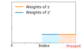
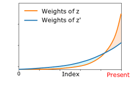
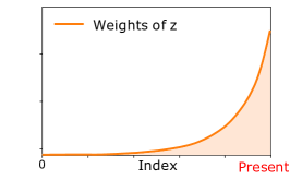
Figure 4: Weights used in the empirical average computations in EWMA (top left), SW (top right), and NEWMA (bottom) algorithms as a function of time. In orange (resp. blue), the weights associated to the average 𝐳tsubscript𝐳𝑡\mathbf{z}_{t} (resp. 𝐳tsubscriptsuperscript𝐳𝑡\mathbf{z}^{\prime}_{t}).
Table 1: Computational and memory footprint of the main algorithms discussed in this article. CΨsubscript𝐶ΨC_{\Psi} (resp. MΨsubscript𝑀ΨM_{\Psi}) indicates time complexity (resp. the memory requirement) of computing ΨΨ\Psi (see Sec. 4.3). In Scan-B𝐵B, N𝑁N is the number of windows of size B𝐵B considered.
ALGORITHM TIME MEMORY
EWMA (Alg. 1) CΨ+msubscript𝐶Ψ𝑚C_{\Psi}+m m+MΨ𝑚subscript𝑀Ψm+M_{\Psi}
Model-free:
SW (Alg. 2) CΨ+msubscript𝐶Ψ𝑚C_{\Psi}+m Bd+m+MΨ𝐵𝑑𝑚subscript𝑀ΨBd+m+M_{\Psi}
Scan-B𝐵B [30] NBd𝑁𝐵𝑑NBd NBd𝑁𝐵𝑑NBd
NEWMA (Alg. 3) CΨ+msubscript𝐶Ψ𝑚C_{\Psi}+m m+MΨ𝑚subscript𝑀Ψm+M_{\Psi}

In this section we introduce the proposed algorithm NEWMA (Alg. 3), give some of its basic theoretical properties, and derive heuristics to choose some of its hyperparameters.

3.1 The NEWMA algorithm

NEWMA is based on the following idea: compute two EWMA statistics with different forgetting factors λ<Λ𝜆Λ\lambda<\Lambda, and raise an alarm when these two statistics are too far apart. The intuition behind this idea is simple: the statistic with the larger forgetting factor ΛΛ\Lambda gives “more importance” to recent samples than the one that uses λ𝜆\lambda, so the distance between them should increase in case of a recent change.

To help illustrate this, in Fig. 4, we schematically represent the three different weighting procedures of EWMA, SW and NEWMA. As mentioned in the introduction: 1) EWMA computes recursively one average with exponential weights, but requires prior knowledge of a control value to compare with; 2) SW computes averages in two different time windows, but needs to keep in memory the last 2B2𝐵2B samples for this purpose; and 3) by recursively computing two exponentially weighted averages with different forgetting factors, NEWMA compares pools of recent and old samples (see Prop. 1 just below), but does not need to store them in memory. By this point of view, NEWMA relies on the same principle as SW (which will be our main baseline for comparison), but is expected to be more efficient computationally.

Remark 1.

Unlike SW, the NEWMA algorithm is very specific to the use of generalized moments. Indeed, since SW has access to the raw data in two time windows, it could potentially estimate any generic metric between batches of samples, such as the KL-divergence, the total variation [3] or the Wasserstein distance [9], although we mentioned in the introduction their potential issues in high dimension. On the contrary, NEWMA does not have access to the raw data, and is specifically based on computing on-the-fly generalized moments with different forgetting factors. Although a finite number of generalized moments can never capture all information for all probability distributions, we will see in Section 4 how randomly chosen moments approximate the MMD, which is a true metric.

In Table 1, we compare their computational costs, along with the Scan-B𝐵B algorithm of [30] described in Sec. 2 and used in our experiments. We can see that the complexity of MA and Scan-B𝐵B is generally dominated by the storage of the raw data, while NEWMA has the same complexity as EWMA. A crucial factor is the computational cost of ΨΨ\Psi, see Sec. 4 for the case of kernel random features.

3.2 Preliminary analysis of NEWMA

Let us formalize a bit the intuition behind NEWMA, by showing first that it indeed computes implicitely a difference between empirical averages in two different time windows. The following, simple proposition is showed in App. B.1 in the supplementary material.

Proposition 1 (Rewriting the detection statistic).

Define B=B(λ,Λ)=def.log(Λ/λ)log((1λ)/(1Λ))𝐵𝐵𝜆Λsuperscriptdef.Λ𝜆1𝜆1ΛB=B(\lambda,\Lambda)\stackrel{{\scriptstyle\textrm{{def.}}}}{{=}}\left\lceil\frac{\log\left(\Lambda/\lambda\right)}{\log\left((1-\lambda)/(1-\Lambda)\right)}\right\rceil, and run NEWMA (Alg. 3). Then, for any t>B𝑡𝐵t>B,

𝐳t𝐳t=C(i=tB+1taiΨ(xi)(b0𝐳0+i=1tBbiΨ(xi))),subscript𝐳𝑡subscriptsuperscript𝐳𝑡𝐶superscriptsubscript𝑖𝑡𝐵1𝑡subscript𝑎𝑖Ψsubscript𝑥𝑖subscript𝑏0subscript𝐳0superscriptsubscript𝑖1𝑡𝐵subscript𝑏𝑖Ψsubscript𝑥𝑖\mathbf{z}_{t}-\mathbf{z}^{\prime}_{t}=C\left(\sum_{i=t-B+1}^{t}a_{i}\Psi\left(x_{i}\right)-\left(b_{0}\mathbf{z}_{0}+\sum_{i=1}^{t-B}b_{i}\Psi\left(x_{i}\right)\right)\right)\,,

where C=C(λ,Λ)=def.(1λ)B(1Λ)B(0,1)𝐶𝐶𝜆Λsuperscriptdef.superscript1𝜆𝐵superscript1Λ𝐵01C=C(\lambda,\Lambda)\stackrel{{\scriptstyle\textrm{{def.}}}}{{=}}(1-\lambda)^{B}-(1-\Lambda)^{B}\in(0,~{}1), and ai,bisubscript𝑎𝑖subscript𝑏𝑖a_{i},b_{i} are positive numbers which depend only on ΛΛ\Lambda and λ𝜆\lambda, such that i=tB+1tai=1superscriptsubscript𝑖𝑡𝐵1𝑡subscript𝑎𝑖1\sum_{i=t-B+1}^{t}a_{i}=1 and i=0tBbi=1superscriptsubscript𝑖0𝑡𝐵subscript𝑏𝑖1\sum_{i=0}^{t-B}b_{i}=1. The exact expressions of aisubscript𝑎𝑖a_{i} and bisubscript𝑏𝑖b_{i}, can be found in App. B.1.

We see that NEWMA indeed computes the difference between a weighted empirical average of Ψ(xi)Ψsubscript𝑥𝑖\Psi\left(x_{i}\right) over the last B𝐵B samples (where B𝐵B depends on ΛΛ\Lambda and λ𝜆\lambda) and an empirical average over the samples that came before, and therefore that its behavior intuitively mimics that of SW, without the requirement to store raw data in memory.

Using Prop. 1 and simple concentration inequalities, we can show basic probabilistic bounds on the detection statistic. We recall that we designed our algorithm to detect changes through the lens of θΨ(π)=𝔼Ψ(x)subscript𝜃Ψ𝜋𝔼Ψ𝑥\theta_{\Psi}(\pi)=\mathbb{E}\Psi\left(x\right), and defined a pseudometric dΨsubscript𝑑Ψd_{\Psi} in (1). The following proposition shows simple “pointwise” bounds on 𝐳t𝐳tsubscript𝐳𝑡subscriptsuperscript𝐳𝑡\mathbf{z}_{t}-\mathbf{z}^{\prime}_{t} under the null or when there is a change in the last B𝐵B samples. Its proof, based on Mc Diarmid’s concentration inequality, is given in App. B.2 in the supplementary material. We note that such pointwise results are different from usual quantity examined in change-point detection such as the mean time between false alarm, which will be examined in Section 5.1.

Proposition 2 (Bounds at a given time).

Suppose that M=def.supxdΨ(x)<superscriptdef.𝑀subscriptsupremum𝑥superscript𝑑normΨ𝑥M\stackrel{{\scriptstyle\textrm{{def.}}}}{{=}}\sup_{x\in\mathbb{R}^{d}}\left\|\Psi\left(x\right)\right\|<\infty. Let t>B𝑡𝐵t>B be a fixed time point, and ρ(0,1)𝜌01\rho\in(0,1) be some probability of failure.

  1. (i)

    Assume that all samples x1,,xtsubscript𝑥1subscript𝑥𝑡x_{1},\ldots,x_{t} are drawn i.i.d. from π𝜋\pi. Then, with probability at least 1ρ1𝜌1-\rho, we have

    𝐳t𝐳tε1+ε2,normsubscript𝐳𝑡subscriptsuperscript𝐳𝑡subscript𝜀1subscript𝜀2\left\|\mathbf{z}_{t}-\mathbf{z}^{\prime}_{t}\right\|\leq\varepsilon_{1}+\varepsilon_{2}\,, (2)

    where ε1=42M(Λ+λ)log(1/ρ)subscript𝜀142𝑀Λ𝜆1𝜌\varepsilon_{1}=4\sqrt{2}M\sqrt{(\Lambda+\lambda)\log(1/\rho)} and ε2=[(1λ)t(1Λ)t]𝐳0𝔼πΨ(x)subscript𝜀2delimited-[]superscript1𝜆𝑡superscript1Λ𝑡normsubscript𝐳0subscript𝔼𝜋Ψ𝑥\varepsilon_{2}=\left[(1-\lambda)^{t}-(1-\Lambda)^{t}\right]\left\|\mathbf{z}_{0}-\mathbb{E}_{\pi}\Psi\left(x\right)\right\|.

  2. (ii)

    Assume that the last B𝐵B samples are drawn i.i.d. from a distribution πsuperscript𝜋\pi^{\prime}, and all the samples that came before are drawn i.i.d. from π𝜋\pi (that is, xtB,,xti.i.d.πsubscript𝑥𝑡𝐵subscript𝑥𝑡i.i.d.similar-tosuperscript𝜋x_{t-B},\ldots,x_{t}\overset{\emph{i.i.d.}~{}}{\sim}\pi^{\prime} and x1,,xtBi.i.d.πsubscript𝑥1subscript𝑥𝑡𝐵i.i.d.similar-to𝜋x_{1},\ldots,x_{t-B}\overset{\emph{i.i.d.}~{}}{\sim}\pi). Then, with probability at least 1ρ1𝜌1-\rho on the samples, we have

    𝐳t𝐳tCdΨ(π,π)ε1ε2.normsubscript𝐳𝑡subscriptsuperscript𝐳𝑡𝐶subscript𝑑Ψ𝜋superscript𝜋subscript𝜀1subscript𝜀2\left\|\mathbf{z}_{t}-\mathbf{z}^{\prime}_{t}\right\|\geq Cd_{\Psi}(\pi,\pi^{\prime})-\varepsilon_{1}-\varepsilon_{2}\,. (3)

    where C𝐶C is defined as in Prop. 1.

Prop. 2 shows that, when no change occurs (under the null) the detection statistic is bounded with high probability, and when the last B𝐵B samples are distributed “differently” from the previous ones, it is greater than a certain value with high probability. As expected, this difference is measured in terms of the pseudometric dΨsubscript𝑑Ψd_{\Psi}. Note that a more precise statement can be found in App. B.2 in the supplementary material.

Remark 2.

For the sake of clarity, in Prop. 2, (ii)𝑖𝑖(ii), we assumed that exactly the last B𝐵B samples were drawn from πsuperscript𝜋\pi^{\prime}, and that all samples that came before were drawn from π𝜋\pi. In App. B.2, we show a more general result which explicits robustness to slight deviations from this assumption.

3.3 Choice of the forgetting factors ΛΛ\Lambda and λ𝜆\lambda

Although the role of the hyperparameters (Λ,λ)Λ𝜆(\Lambda,\lambda) in the NEWMA algorithm is simple to understand intuitively, it is not clear how to set their values at this stage. On the contrary, the window size B𝐵B in Prop. 1 has a more interpretable meaning: it is the number of recent samples compared with old ones. While it is known that the choice of a window size is a difficult problem and that there is no “universally” good choice, we assume that practitioners are more familiar with choosing a proper window size (sometimes by simple trial-and-error), than they are with choosing forgetting factors that may be difficult to interpret. Hence, in this section, we derive a simple heuristic to set both parameters (Λ,λ)Λ𝜆(\Lambda,\lambda) for a given B𝐵B, which we assume to be given by the user. Methods to guide the selection of B𝐵B are left for future investigations. We build upon the theoretical results of the previous section. We note that choosing a forgetting factor for EWMA is also known to be a difficult problem [11].

Our starting point is the expression of the window size B𝐵B derived in Prop. 1. We first note that a possible parameterization of NEWMA is through B𝐵B and one of the forgetting factors, say ΛΛ\Lambda: given B𝐵B and Λ>1B+1Λ1𝐵1\Lambda>\frac{1}{B+1}, there is a unique λ=λΛ,B1B+1𝜆subscript𝜆Λ𝐵1𝐵1\lambda=\lambda_{\Lambda,B}\leq\frac{1}{B+1} such that log(Λ/λ)log((1λ)/(1Λ))=BΛ𝜆1𝜆1Λ𝐵\frac{\log\left(\Lambda/\lambda\right)}{\log\left((1-\lambda)/(1-\Lambda)\right)}=B in Prop. 1. Indeed, f:xx(1x)B:𝑓maps-to𝑥𝑥superscript1𝑥𝐵f:x\mapsto x(1-x)^{B} is increasing on [0,1B+1]01𝐵1[0,\frac{1}{B+1}] and decreasing on [1B+1,1]1𝐵11[\frac{1}{B+1},1], so the equation f(x)=f(Λ)𝑓𝑥𝑓Λf(x)=f(\Lambda) has exactly one solution in [0,1]01[0,1] besides ΛΛ\Lambda itself. Thus λ𝜆\lambda is uniquely defined by (B,Λ)𝐵Λ(B,\Lambda). We now turn to the choice of ΛΛ\Lambda given a user-defined window size B𝐵B.

From Prop. 2, we can see that the null hypothesis is intuitively distinguishable from the alternative if the bound under the null (2) is smaller than the guaranteed deviation (3) when there is a change, that is, ε1+ε2CdΨ(π,π)ε1ε2,subscript𝜀1subscript𝜀2𝐶subscript𝑑Ψ𝜋superscript𝜋subscript𝜀1subscript𝜀2\varepsilon_{1}+\varepsilon_{2}\leq Cd_{\Psi}(\pi,\pi^{\prime})-\varepsilon_{1}-\varepsilon_{2}\,, which is equivalent to

dΨ(π,π)2(ε1+ε2)/C.subscript𝑑Ψ𝜋superscript𝜋2subscript𝜀1subscript𝜀2𝐶d_{\Psi}(\pi,\pi^{\prime})\geq 2(\varepsilon_{1}+\varepsilon_{2})/C\,.

Since we want our algorithm to be sensitive to the smallest possible change in dΨ(π,π)subscript𝑑Ψ𝜋superscript𝜋d_{\Psi}(\pi,\pi^{\prime}), the previous reasoning suggest that a good choice for ΛΛ\Lambda is to minimize the right-hand side of this expression. Note that ε1subscript𝜀1\varepsilon_{1} depends on the chosen probability of failure ρ𝜌\rho: the smaller it is, the larger dΨ(π,π)subscript𝑑Ψ𝜋superscript𝜋d_{\Psi}(\pi,\pi^{\prime}) should be, however at a mild logarithmic rate.

To obtain our final heuristic, we replace 𝐳0𝔼πΨ(x)normsubscript𝐳0subscript𝔼𝜋Ψ𝑥\left\|\mathbf{z}_{0}-\mathbb{E}_{\pi}\Psi\left(x\right)\right\| by the upper bound 2M2𝑀2M in in the expression of ε2subscript𝜀2\varepsilon_{2}, and we take t=2B𝑡2𝐵t=2B; since ε2t0𝑡absentsubscript𝜀20\varepsilon_{2}\xrightarrow[t\to\infty]{}0 and intuitively we consider that our algorithm must be “applicable” as soon as we have received twice the window size in data. In definitive, for a user-defined B𝐵B, we propose the following heuristic to choose444Note that we discard the multiplicative constants as well as log1ρ1𝜌\log\frac{1}{\rho}, which we found to have negligible effect in practice. ΛΛ\Lambda:

Λ=argminΛ(1B+1,1)λΛ,B+Λ+(1λΛ,B)2B(1Λ)2B(1λΛ,B)B(1Λ)B,superscriptΛsubscriptargminΛ1𝐵11subscript𝜆Λ𝐵Λsuperscript1subscript𝜆Λ𝐵2𝐵superscript1Λ2𝐵superscript1subscript𝜆Λ𝐵𝐵superscript1Λ𝐵\Lambda^{\star}\!\!=\!\!\operatorname*{arg\,min}_{\Lambda\in(\frac{1}{B+1},1)}\!\!\frac{\sqrt{\lambda_{\Lambda,B}+\Lambda}+(1-\lambda_{\Lambda,B})^{2B}-(1-\Lambda)^{2B}}{(1-\lambda_{\Lambda,B})^{B}-(1-\Lambda)^{B}},

where we recall that λΛ,Bsubscript𝜆Λ𝐵\lambda_{\Lambda,B} is the unique λ𝜆\lambda such that log(Λ/λ)log((1λ)/(1Λ))=BΛ𝜆1𝜆1Λ𝐵\frac{\log\left(\Lambda/\lambda\right)}{\log\left((1-\lambda)/(1-\Lambda)\right)}=B. Once ΛsuperscriptΛ\Lambda^{\star} is chosen, we naturally set the corresponding λ=λΛ,Bsuperscript𝜆subscript𝜆superscriptΛ𝐵\lambda^{\star}=\lambda_{\Lambda^{\star},B} to respect the window size B𝐵B. We note that ΛsuperscriptΛ\Lambda^{\star} and λsuperscript𝜆\lambda^{\star} do not have explicit expressions with respect to B𝐵B, but they can easily be approximated by simple one-dimensional optimization schemes. In practice, given ΛΛ\Lambda and B𝐵B, we find λΛ,Bsubscript𝜆Λ𝐵\lambda_{\Lambda,B} with a simple gradient descent, and we select ΛsuperscriptΛ\Lambda^{\star} with an exhaustive search over a fine grid of [0,1]01[0,1].

This heuristic is seen to yield good results in practice in many situations. We leave for future work a more rigorous proof of optimality in simpler settings (e.g., Gaussian data).

4 Choice of ΨΨ\Psi: Random Features

Let us now turn to the important choice of the embedding ΨΨ\Psi. We recall that ΨΨ\Psi is user-defined, and that the algorithms studied in this paper are sensitive to variations in the collection of generalized moments θΨ(π)=𝔼πΨ(x)subscript𝜃Ψ𝜋subscript𝔼𝜋Ψ𝑥\theta_{\Psi}(\pi)=\mathbb{E}_{\pi}\Psi\left(x\right). As mentioned before, if the practitioner knows in advance which statistic is susceptible to vary, then ΨΨ\Psi can be chosen accordingly. However, one does not necessarily have a priori knowledge on the nature of the change. In this section, we describe a generic embedding related to kernel metric on distributions.

4.1 Maximum Mean Discrepancy

For most ΨΨ\Psi, dΨ(π,π)subscript𝑑Ψ𝜋superscript𝜋d_{\Psi}(\pi,\pi^{\prime}) is only a pseudometric on probability distributions: for instance, when Ψ(x)=xΨ𝑥𝑥\Psi\left(x\right)=x, it can only distinguish distributions that have different means. Ideally however, one would like dΨsubscript𝑑Ψd_{\Psi} to be a true metric, that is, we want dΨ(π,π)=0subscript𝑑Ψ𝜋superscript𝜋0d_{\Psi}(\pi,\pi^{\prime})=0 if, and only if, π=π𝜋superscript𝜋\pi=\pi^{\prime}. Unfortunately, for any mapping ΨΨ\Psi with values in a finite-dimensional space, dΨsubscript𝑑Ψd_{\Psi} cannot be a true metric—otherwise θΨ()subscript𝜃Ψ\theta_{\Psi}(\cdot) would be an isometry between an infinite-dimensional space and a finite-dimensional space. In particular, this is the case for any ΨΨ\Psi used in practice. Luckily, as described in the rest of this section, an interesting strategy is to leverage the Random Features methodology to obtain random embeddings ΨΨ\Psi such that dΨ(π,π)subscript𝑑Ψ𝜋superscript𝜋d_{\Psi}(\pi,\pi^{\prime}) approximates a true metric between distributions with high probability.

A possible choice for such a metric is the Maximum Mean Discrepancy (MMD, [22]). Given a positive definite kernel κ𝜅\kappa on dsuperscript𝑑\mathbb{R}^{d}, take \mathcal{H} as the Reproducing Kernel Hilbert Space (RKHS555A good introduction to the theory of RKHSs is e.g. [5]) associated to κ𝜅\kappa. If we set Ψ(x)=κ(x,)Ψ𝑥𝜅𝑥\Psi\left(x\right)=\kappa(x,\cdot) and =\left\|\cdot\right\|=\left\|\cdot\right\|_{\mathcal{H}}, then, in our notation, dΨ(π,π)=𝔼πκ(x,)𝔼πκ(x,)subscript𝑑Ψ𝜋superscript𝜋subscriptnormsubscript𝔼𝜋𝜅𝑥subscript𝔼𝜋𝜅𝑥d_{\Psi}(\pi,\pi^{\prime})=\left\|\mathbb{E}_{\pi}\kappa(x,\cdot)-\mathbb{E}_{\pi}\kappa(x,\cdot)\right\|_{\mathcal{H}} is the MMD between π𝜋\pi and πsuperscript𝜋\pi^{\prime}, that we denote by MMD(π,π)MMD𝜋superscript𝜋\textrm{{MMD}}(\pi,\pi^{\prime}). When the kernel κ𝜅\kappa is characteristic, it is a true metric. Many conditions have been formulated over the years for κ𝜅\kappa to be characteristic [40], and for instance the Gaussian kernel is characteristic. First introduced in the context of two-sample test, the MMD appears quite naturally in the context of kernel change-point detection [25, 19] and in particular the online Scan-B𝐵B algorithm [30].

4.2 Random Features

In practice, since Ψ(x)=κ(x,)Ψ𝑥𝜅𝑥\Psi\left(x\right)=\kappa(x,\cdot) cannot be stored in memory to compute the theoretical MMD, empirical estimates thereof are used. Such estimates usually make use of the so-called kernel trick, and require the computation of a U𝑈U-statistic depending on populations drawn from both distributions: it is for instance the method used in the kernel Scan-B𝐵B algorithm [30]. Since we do not want to store samples when NEWMA is running, least of all perform costly computations on these samples, we resort to kernel Random Features (RF, [36]), exploiting the simple fact the Euclidean distance between averaged random features approximates the MMD with high probability over the features. RFs and MMD have been combined together before, for accelerating the estimation of the MMD [42] or as a mean to design random projections of distributions in an inverse-problem context [23]. We also note that alternatives to RFs have been studied in the MMD literature [10], which is an interesting path for future work.

Let us briefly describe the RF machinery. Assume that the kernel κ𝜅\kappa can be written as κ(x,x)=𝔼𝝎Γϕ𝝎(x)ϕ𝝎(x)¯𝜅𝑥superscript𝑥subscript𝔼similar-to𝝎Γsubscriptitalic-ϕ𝝎𝑥¯subscriptitalic-ϕ𝝎superscript𝑥\kappa(x,x^{\prime})=\mathbb{E}_{{\boldsymbol{\omega}}\sim\Gamma}{\phi_{{\boldsymbol{\omega}}}}(x)\overline{{\phi_{{\boldsymbol{\omega}}}}(x^{\prime})} for a family of functions ϕ𝝎:d:subscriptitalic-ϕ𝝎superscript𝑑{\phi_{{\boldsymbol{\omega}}}}:\mathbb{R}^{d}\to\mathbb{C} parameterized by 𝝎q𝝎superscript𝑞{\boldsymbol{\omega}}\in\mathbb{R}^{q}, and a probability distribution ΓΓ\Gamma on qsuperscript𝑞\mathbb{R}^{q}. This is for instance the case for all translation-invariant kernels [4, 36]: by Bochner’s theorem, they can all be written under this form for complex exponentials ϕ𝝎(x)=ei𝝎xsubscriptitalic-ϕ𝝎𝑥superscript𝑒isuperscript𝝎top𝑥{\phi_{{\boldsymbol{\omega}}}}(x)=e^{\textrm{i}{\boldsymbol{\omega}}^{\top}x} and some symmetric distribution ΓΓ\Gamma. Using complex exponentials as ϕ𝝎subscriptitalic-ϕ𝝎{\phi_{{\boldsymbol{\omega}}}} is usually referred to as Random Fourier Features (RFF). The most classical example is the Gaussian kernel κ(x,x)=exx22σ2𝜅𝑥superscript𝑥superscript𝑒superscriptnorm𝑥superscript𝑥22superscript𝜎2\kappa(x,x^{\prime})=e^{-\frac{\left\|x-x^{\prime}\right\|^{2}}{2\sigma^{2}}}, which is written under this form for a Gaussian distribution Γ=𝒩(0,σ2Id)Γ𝒩0superscript𝜎2Id\Gamma=\mathcal{N}(0,\sigma^{-2}\textrm{{Id}}).

For some (large) integer m𝑚m\in\mathbb{N}, the RF paradigm consists in drawing m𝑚m parameters 𝝎1,,𝝎mi.i.d.Γsubscript𝝎1subscript𝝎𝑚i.i.d.similar-toΓ{\boldsymbol{\omega}}_{1},\ldots,{\boldsymbol{\omega}}_{m}\overset{\emph{i.i.d.}~{}}{\sim}\Gamma and defining Ψ:dm:Ψsuperscript𝑑superscript𝑚\Psi:\mathbb{R}^{d}\to\mathbb{C}^{m} as

Ψ(x)=def.1m(ϕ𝝎j(x))j=1m,superscriptdef.Ψ𝑥1𝑚superscriptsubscriptsubscriptitalic-ϕsubscript𝝎𝑗𝑥𝑗1𝑚\Psi\left(x\right)\stackrel{{\scriptstyle\textrm{{def.}}}}{{=}}\frac{1}{\sqrt{m}}\left(\phi_{{\boldsymbol{\omega}}_{j}}(x)\right)_{j=1}^{m}\,, (4)

and taking \left\|\cdot\right\| as the classical Hermitian norm on msuperscript𝑚\mathbb{C}^{m}. A simple computation (see the proof of Prop. 3 in App. B.3) then shows that dΨ(π,π)MMD(π,π)subscript𝑑Ψ𝜋superscript𝜋MMD𝜋superscript𝜋d_{\Psi}(\pi,\pi^{\prime})\approx\textrm{{MMD}}(\pi,\pi^{\prime}), with high probability over the 𝝎jsubscript𝝎𝑗{\boldsymbol{\omega}}_{j}. With this choice of ΨΨ\Psi, we have the following result similar to Prop. 2.

Proposition 3 (EWMA-RF pointwise detection).

Suppose that supx,𝛚|ϕ𝛚(x)|Msubscriptsupremum𝑥𝛚subscriptitalic-ϕ𝛚𝑥𝑀\sup_{x,{\boldsymbol{\omega}}}\left\lvert{\phi_{{\boldsymbol{\omega}}}}(x)\right\rvert\leq M. Define Ψ()Ψ\Psi\left(\cdot\right) as in Eq. (4). Let ρ(0,1)𝜌01\rho\in(0,1) be a probability of failure. Suppose that the assumptions of Prop. 2, (ii)𝑖𝑖(ii) hold. Then, with probability at least 12ρ12𝜌1-2\rho on both samples xisubscript𝑥𝑖x_{i} and parameters 𝛚jsubscript𝛚𝑗{\boldsymbol{\omega}}_{j}, it holds that

𝐳t𝐳tC(MMD2(π,π)εm)+12ε1ε2,normsubscript𝐳𝑡subscriptsuperscript𝐳𝑡𝐶superscriptsubscriptsuperscriptMMD2𝜋superscript𝜋subscript𝜀𝑚12subscript𝜀1subscript𝜀2\displaystyle\left\|\mathbf{z}_{t}-\mathbf{z}^{\prime}_{t}\right\|\geq C\Big{(}\textrm{{MMD}}^{2}(\pi,\pi^{\prime})-\varepsilon_{m}\Big{)}_{+}^{\frac{1}{2}}-\varepsilon_{1}-\varepsilon_{2}\,, (5)

where (x)+=max(x,0)subscript𝑥𝑥0(x)_{+}=\max(x,0) and εm=22M2mlog1ρsubscript𝜀𝑚22superscript𝑀2𝑚1𝜌\varepsilon_{m}=\tfrac{2\sqrt{2}M^{2}}{\sqrt{m}}\sqrt{\log\tfrac{1}{\rho}}.

By the previous proposition, if the MMD between π𝜋\pi and πsuperscript𝜋\pi^{\prime} is large, then with high probability so is the deviation of 𝐳t𝐳tnormsubscript𝐳𝑡subscriptsuperscript𝐳𝑡\left\|\mathbf{z}_{t}-\mathbf{z}^{\prime}_{t}\right\|. The additional error εmsubscript𝜀𝑚\sqrt{\varepsilon_{m}} is of the order of the previous error ε1subscript𝜀1\varepsilon_{1} if m=𝒪((Λ+λ)2)𝑚𝒪superscriptΛ𝜆2m=\mathcal{O}\left((\Lambda+\lambda)^{-2}\right).

The choice of a good kernel κ𝜅\kappa is a notoriously difficult problem. Ideally, one would choose it so as to maximize MMD(π,π)MMD𝜋superscript𝜋\textrm{{MMD}}(\pi,\pi^{\prime}), however neither π𝜋\pi nor πsuperscript𝜋\pi^{\prime} are known in advance in our setting. In practice, we use the Gaussian kernel. Having access to some initial training data, we choose the bandwidth σ𝜎\sigma using the median trick as in [30]. We leave for future work more involved methods for kernel selection [46].

4.3 Fast random features and computational cost

A crucial factor in the application of NEWMA is the complexity of the mapping ΨΨ\Psi, both in computation time or memory footprint of the parameters necessary to compute it, which we respectively denoted by CΨsubscript𝐶ΨC_{\Psi} and MΨsubscript𝑀ΨM_{\Psi} in Table 1. For usual RFFs [36], computing Ψ(x)Ψ𝑥\Psi\left(x\right) requires storing the dense matrix of frequencies 𝝎jdsubscript𝝎𝑗superscript𝑑{\boldsymbol{\omega}}_{j}\in\mathbb{R}^{d}, and performing a costly matrix-vector product. Therefore, in this case both CΨsubscript𝐶ΨC_{\Psi} and MΨsubscript𝑀ΨM_{\Psi} scale as 𝒪(md)𝒪𝑚𝑑\mathcal{O}\left(md\right), which somehow mitigates the computations advantages of using NEWMA over more costly methods.

However, a large body of work is dedicated to accelerate the computation of such random features. For instance, the Fastfood (FF) approximation [29] reduces the time complexity to 𝒪(mlogd)𝒪𝑚𝑑\mathcal{O}\left(m\log d\right) and memory to 𝒪(m)𝒪𝑚\mathcal{O}\left(m\right).

More strikingly, in [38], the authors build an Optical Processing Unit (OPU), to which we had had access for our experiments (Sec. 6), that computes random features in 𝒪(1)𝒪1\mathcal{O}\left(1\right) and eliminates the need to store the random matrix. Let us briefly describe how the OPU operates. To compute some random mapping (ϕ𝝎j(x))j=1msuperscriptsubscriptsubscriptitalic-ϕsubscript𝝎𝑗𝑥𝑗1𝑚\left(\phi_{{\boldsymbol{\omega}}_{j}}(x)\right)_{j=1}^{m}, the signal x𝑥x is first encoded into a light beam using a Digital Micromirror Device (DMD). The beam is then focused and scattered through a layer of heterogeneous material, which corresponds to performing many random linear operations on the underlying signal. Then, the amplitude is measured by a camera, which adds a non-linearity on the output. The corresponding kernel, which is imposed by the physical device, is an elliptic kernel whose expression is given in [38]. We refer the reader to [38, 15] for complete details on the process. In addition to being able to compute RFs in 𝒪(1)𝒪1\mathcal{O}\left(1\right) for m,d𝑚𝑑m,d in the order of millions (for current hardware), OPUs are also significantly less energy-consuming than classical GPUs.

We summarize the respective complexities of these three approaches in Table 2.

Table 2: Time complexity CΨsubscript𝐶ΨC_{\Psi} and memory requirement MΨsubscript𝑀ΨM_{\Psi} for different Random Features schemes.
RFF FF OPU
CΨsubscript𝐶ΨC_{\Psi} 𝒪(md)𝒪𝑚𝑑\mathcal{O}\left(md\right) 𝒪(mlogd)𝒪𝑚𝑑\mathcal{O}\left(m\log d\right) 𝒪(1)𝒪1\mathcal{O}\left(1\right)
MΨsubscript𝑀ΨM_{\Psi} 𝒪(md)𝒪𝑚𝑑\mathcal{O}\left(md\right) 𝒪(m)𝒪𝑚\mathcal{O}\left(m\right) 𝒪(1)𝒪1\mathcal{O}\left(1\right)

5 Setting the threshold

In this section, we go back to the case of any general mapping ΨΨ\Psi. An important question for any change-point detection method that tracks a statistic along time is how to set the threshold τ𝜏\tau above which a change-point is detected. In this section, we begin by adapting to NEWMA two classical approaches that use the property of the algorithm under the null hypothesis. However, while they are interesting in their own right, these approaches generally cannot be directly used in practice since they require to know the in-control distribution π𝜋\pi. Hence we describe an efficient numerical procedure to dynamically adapt the threshold during a continuous run with multiple changes.

5.1 Mean time between false alarms

A classical method to set the threshold τ𝜏\tau is to adjust a desired mean time between false alarms under the null, defined as T¯=def.𝔼[inf{t|t is flagged}],superscriptdef.¯𝑇𝔼delimited-[]infimumconditional-set𝑡𝑡 is flagged\overline{T}\stackrel{{\scriptstyle\textrm{{def.}}}}{{=}}\mathbb{E}\left[\inf\left\{t~{}|~{}t\text{ is flagged}\right\}\right], where the expectation is over the samples under the null (that is, drawn i.i.d. from some distribution π𝜋\pi). In the literature, it is often referred to as the Average Run Length (ARL) under control.

Unless strong assumptions are made on π𝜋\pi, it is often impossible to derive a closed-form expression for the ARL. A possible strategy is to estimate it using some training data, however this method is impractical in a continuous run with multiple changes. We will derive simpler strategies in the next sections. For theoretical purposes, we nevertheless show that it is possible to adapt the Markov chain-based proof developed for classical EWMA in [17] to NEWMA: this method derives an expression for the ARL – however, as we mentioned, it rarely has a closed-form expression and requires unreasonable prior knowledge. Unlike the results from the previous sections, our analysis is valid without any boundedness assumption on ΨΨ\Psi. We present our theorem in the unidimensional case =\mathcal{H}=\mathbb{R}.

Theorem 4 (Average Run Length of NEWMA).

Assume that Ψ:d:Ψsuperscript𝑑\Psi:\mathbb{R}^{d}\to\mathbb{R} maps to a unidimensional space, and assume that Ψ(X)Ψ𝑋\Psi\left(X\right) has a density under the null. Denote by F(x)=def.Xπ(Ψ(X)x)superscriptdef.𝐹𝑥subscriptsimilar-to𝑋𝜋Ψ𝑋𝑥F(x)\stackrel{{\scriptstyle\textrm{{def.}}}}{{=}}\mathbb{P}_{X\sim\pi}\left(\Psi\left(X\right)\leq x\right) its cumulative distribution function. For any ε>0𝜀0\varepsilon>0, define {a1,aM}subscript𝑎1subscript𝑎𝑀\{a_{1},\ldots a_{M}\} an ε𝜀\varepsilon-grid of [1/ε,1/ε]1𝜀1𝜀[-1/\varepsilon,1/\varepsilon], that is, M=def.2ε2superscriptdef.𝑀2superscript𝜀2M\stackrel{{\scriptstyle\textrm{{def.}}}}{{=}}\left\lceil\frac{2}{\varepsilon^{2}}\right\rceil and ai=def.(i1)ε1/εsuperscriptdef.subscript𝑎𝑖𝑖1𝜀1𝜀a_{i}\stackrel{{\scriptstyle\textrm{{def.}}}}{{=}}(i-1)\varepsilon-1/\varepsilon. Then, consider the list of all couples 𝐮k=(ai,aj)subscript𝐮𝑘subscript𝑎𝑖subscript𝑎𝑗\mathbf{u}_{k}=(a_{i},a_{j}) such that |aiaj|τsubscript𝑎𝑖subscript𝑎𝑗𝜏\left\lvert a_{i}-a_{j}\right\rvert\leq\tau, indexed by 1kK1𝑘𝐾1\leq k\leq K for some KM2𝐾superscript𝑀2K\leq M^{2} that depends on ε𝜀\varepsilon and τ𝜏\tau. For any 𝐮k1=(ai1,aj1)subscript𝐮subscript𝑘1subscript𝑎subscript𝑖1subscript𝑎subscript𝑗1\mathbf{u}_{k_{1}}=(a_{i_{1}},a_{j_{1}}) and 𝐮k2=(ai2,aj2)subscript𝐮subscript𝑘2subscript𝑎subscript𝑖2subscript𝑎subscript𝑗2\mathbf{u}_{k_{2}}=(a_{i_{2}},a_{j_{2}}), define

pk1k2={F(u2)F(u1)if u1<u20otherwise.subscript𝑝subscript𝑘1subscript𝑘2cases𝐹subscript𝑢2𝐹subscript𝑢1if u1<u20otherwise.p_{k_{1}k_{2}}=\begin{cases}F(u_{2})-F(u_{1})&\quad\text{if $u_{1}<u_{2}$}\\ 0&\quad\text{otherwise.}\end{cases}

where

{u1=max(1Λ(ai2(1Λ)ai1ε/2),1λ(aj2(1λ)aj1ε/2)),u2=min(1Λ(ai2(1Λ)ai1+ε/2),1λ(aj2(1λ)aj1+ε/2)).\begin{cases}u_{1}&=\max\Big{(}\frac{1}{\Lambda}(a_{i_{2}}-(1-\Lambda)a_{i_{1}}-\varepsilon/2),\\ &\qquad\qquad\frac{1}{\lambda}(a_{j_{2}}-(1-\lambda)a_{j_{1}}-\varepsilon/2)\Big{)}\,,\\ u_{2}&=\min\Big{(}\frac{1}{\Lambda}(a_{i_{2}}-(1-\Lambda)a_{i_{1}}+\varepsilon/2),\\ &\qquad\qquad\frac{1}{\lambda}(a_{j_{2}}-(1-\lambda)a_{j_{1}}+\varepsilon/2)\Big{)}\,.\end{cases}

Define the matrix 𝐏=[pk1k2]k1,k2=1K𝐏superscriptsubscriptdelimited-[]subscript𝑝subscript𝑘1subscript𝑘2subscript𝑘1subscript𝑘21𝐾\mathbf{P}=[p_{k_{1}k_{2}}]_{k_{1},k_{2}=1}^{K}. Then, we have

T¯=1+1limε0𝐞1𝐏𝟏K,¯𝑇1subscript1subscript𝜀0superscriptsubscript𝐞1topsuperscript𝐏subscript1𝐾\overline{T}=1+\sum_{\ell\geq 1}\lim_{\varepsilon\to 0}\mathbf{e}_{1}^{\top}\mathbf{P}^{\ell}\mathbf{1}_{K}\,, (6)

where T¯¯𝑇\overline{T} is the ARL of NEWMA, 𝟏=[1,,1]1superscript11top\mathbf{1}=[1,\ldots,1]^{\top} and 𝐞1=[1,0,,0]subscript𝐞1superscript100top\mathbf{e}_{1}=[1,0,\ldots,0]^{\top}.

In App. A.1 we prove a (quite notation-heavy) more general version of this theorem in the case where Ψ:dm:Ψsuperscript𝑑superscript𝑚\Psi:\mathbb{R}^{d}\to\mathbb{R}^{m} is a multidimensional map, in which case the grid {ai}subscript𝑎𝑖\{a_{i}\} is replaced by an ε𝜀\varepsilon-net.

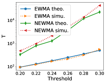
From (6), it is difficult to describe precisely the effect of the different parameters of NEWMA on its ARL. Naturally, the larger the threshold τ𝜏\tau is, the higher the ARL is (in Theorem 4, a higher threshold results in a larger K𝐾K). Similarly, a larger window size B𝐵B in Proposition 1 intuitively results in a “smoother” algorithm and a higher ARL, although it is less obvious in the theoretical expression. In simple cases where F𝐹F is known, it is possible to perform numerical simulations using (6). In general, it is impossible to exchange the infinite sum “1subscript1\sum_{\ell\geq 1}” and the limit “ε0𝜀0\varepsilon\to 0” in (6), as this would require uniform convergence. However, in practice, for numerical purpose, we can fix a small ε>0𝜀0\varepsilon>0 and use the identity 0𝐀=(Id𝐀)1subscript0superscript𝐀superscriptId𝐀1\sum_{\ell\geq 0}\mathbf{A}^{\ell}=(\textrm{{Id}}-\mathbf{A})^{-1} to approximate T¯𝐞1(Id𝐏)1𝟏¯𝑇superscriptsubscript𝐞1topsuperscriptId𝐏11\overline{T}\approx\mathbf{e}_{1}^{\top}(\textrm{{Id}}-\mathbf{P})^{-1}\mathbf{1}. We illustrate this principle in Fig. 5 with a Gaussian distribution Ψ(X)𝒩(0,1)similar-toΨ𝑋𝒩01\Psi\left(X\right)\sim\mathcal{N}(0,1), using respectively Th. 4 and the original approach by [17], as well as numerical simulations of runs on synthetic data. As we mentioned before, when the in-control distribution π𝜋\pi is not known (or, more precisely, when the cumulative distribution function F𝐹F is not known), Th. 4 cannot be directly applied. In some cases [30], one can obtain an asymptotic expression for T¯¯𝑇\overline{T} when τ𝜏\tau\to\infty which does not depend on π𝜋\pi, which we leave for future work.

Refer to caption
Figure 5: Comparison of the theoretical and observed values of T¯¯𝑇\overline{T} for NEWMA (resp. EWMA) with respect to τ𝜏\tau, with π=𝒩(0,1)𝜋𝒩01\pi=\mathcal{N}(0,1), Ψ(x)=xΨ𝑥𝑥\Psi\left(x\right)=x, Λ=2101Λ2superscript101\Lambda=2\cdot 10^{-1} and λ=101𝜆superscript101\lambda=10^{-1}. The simulations are averaged over 100010001000 runs, the theoretical expression is obtained with Th. 4 (resp. [17]) with a grid of precision ε=2102𝜀2superscript102\varepsilon=2\cdot 10^{-2}. Here we do not qualitatively compare EWMA and NEWMA, but rather illustrate the quality of the theoretical approximations for the ARL.

5.2 Asymptotic distribution under the null

Another, arguably simpler approach to set the threshold τ𝜏\tau is to derive the distribution of 𝐳t𝐳tnormsubscript𝐳𝑡superscriptsubscript𝐳𝑡\left\|\mathbf{z}_{t}-\mathbf{z}_{t}^{\prime}\right\| under the null, and set τ𝜏\tau to obtain a desired probability of exceeding it. In this section, we derive an asymptotic result on the distribution of this statistic when λ0𝜆0\lambda\to 0 and t𝑡t\to\infty. Unlike Prop. 2, where ΨΨ\Psi is assumed uniformly bounded, it relies on the slightly weaker assumption that ΨΨ\Psi has a finite fourth order moment.

Theorem 5 (Convergence under the null).

Assume c=Λ/λ>1𝑐Λ𝜆1c=\Lambda/\lambda>1 is fixed, and let Λ0Λ0\Lambda\to 0, with t2λlog1λ𝑡2𝜆1𝜆t\geq\frac{2}{\lambda}\log\frac{1}{\lambda}. Assume that all samples xisubscript𝑥𝑖x_{i} are drawn i.i.d. from π𝜋\pi. Suppose that 𝔼πΨ(x)4<+subscript𝔼𝜋superscriptnormΨ𝑥4\mathbb{E}_{\pi}\left\|\Psi\left(x\right)\right\|^{4}<+\infty. Set μ=def.𝔼πΨ(x)superscriptdef.𝜇subscript𝔼𝜋Ψ𝑥\mu\stackrel{{\scriptstyle\textrm{{def.}}}}{{=}}\mathbb{E}_{\pi}\Psi\left(x\right), and K(x,x)=def.Ψ(x)μ,Ψ(x)μsuperscriptdef.𝐾𝑥superscript𝑥subscriptΨ𝑥𝜇Ψsuperscript𝑥𝜇K(x,x^{\prime})\stackrel{{\scriptstyle\textrm{{def.}}}}{{=}}\left\langle\Psi\left(x\right)-\mu,\Psi\left(x^{\prime}\right)-\mu\right\rangle_{\mathcal{H}}.

Define the eigenvalues and eigenvectors of K𝐾K in L2(π)superscript𝐿2𝜋L^{2}(\pi), i.e., define ξ0subscript𝜉0\xi_{\ell}\geq 0 and ψL2(π)subscript𝜓superscript𝐿2𝜋\psi_{\ell}\in L^{2}(\pi) such that K(x,x)=1ξψ(x)ψ(x)𝐾𝑥superscript𝑥subscript1subscript𝜉subscript𝜓𝑥subscript𝜓superscript𝑥K(x,x^{\prime})=\sum_{\ell\geq 1}\xi_{\ell}\psi_{\ell}(x)\psi_{\ell}(x^{\prime}) and ψ,ψL2(π)=1=subscriptsubscript𝜓subscript𝜓superscriptsuperscript𝐿2𝜋subscript1superscript\left\langle\psi_{\ell},\psi_{\ell^{\prime}}\right\rangle_{L^{2}(\pi)}=1_{\ell=\ell^{\prime}}.

Then,

1λ𝐳t𝐳t2η0Y=def.(1c)22(1+c)1ξW2,𝜂01𝜆superscriptnormsubscriptsuperscript𝐳𝑡subscript𝐳𝑡2𝑌superscriptdef.superscript1𝑐221𝑐subscript1subscript𝜉superscriptsubscript𝑊2\frac{1}{\lambda}\left\|\mathbf{z}^{\prime}_{t}-\mathbf{z}_{t}\right\|^{2}\xrightarrow[\eta\to 0]{\mathcal{L}}Y\stackrel{{\scriptstyle\textrm{{def.}}}}{{=}}\frac{(1-c)^{2}}{2(1+c)}\sum_{\ell\geq 1}\xi_{\ell}W_{\ell}^{2}\,, (7)

where (W)1subscriptsubscript𝑊1\left(W_{\ell}\right)_{\ell\geq 1} is an infinite sequence of independent standard normal random variables.
Refer to caption
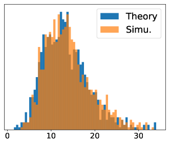
Figure 6: Distribution of 1λ𝐳t𝐳t21𝜆superscriptnormsubscript𝐳𝑡subscriptsuperscript𝐳𝑡2\frac{1}{\lambda}\left\|\mathbf{z}_{t}-\mathbf{z}^{\prime}_{t}\right\|^{2} when λ0𝜆0\lambda\to 0 as predicted by Th. 5, on a toy example. Namely, π𝜋\pi is the uniform distribution on [0,1]01[0,1] and Ψ(x)=[ξψ()]=130Ψ𝑥superscriptsubscriptdelimited-[]subscript𝜉subscript𝜓130\Psi(x)=\left[\sqrt{\xi_{\ell}}\psi_{\ell}(\cdot)\right]_{\ell=1}^{30} is defined as a collection of eigenfunctions ψ(x)=2cos(2πx)subscript𝜓𝑥22𝜋𝑥\psi_{\ell}(x)=\sqrt{2}\cos(2\pi\ell x), where the eigenvalues (ξ)=130superscriptsubscriptsubscript𝜉130\left(\xi_{\ell}\right)_{\ell=1}^{30} are randomly generated. We perform 100010001000 simulations of both Eq. (7) and NEWMA with Λ=2102,λ=102formulae-sequenceΛ2superscript102𝜆superscript102\Lambda=2\cdot 10^{-2},\lambda=10^{-2}.

The proof, given in App. A.2, follows closely [39] (Sec. 5.5.2) adapted to our setting, with the use of a multivariate version of Lindeberg’s central limit theorem (recalled as Th. 12 in the supplementary) instead of the classical Central Limit Theorem. Th. 5 allows to set the threshold τ𝜏\tau if the eigenvalues ξsubscript𝜉\xi_{\ell} are (approximately) known, for instance they can be estimated using the Gram matrix of K𝐾K on training data [21], which we leave for future work. In Fig. 6, we illustrate the result on a toy example.

5.3 Choice of an adaptive threshold

Stream of detection statistics Stsubscript𝑆𝑡S_{t}, estimation rate 0<α<10𝛼10<\alpha<1, coefficient a𝑎a
Initialize μ0=0subscript𝜇00\mu_{0}=0 (mean), μ0(2)=0subscriptsuperscript𝜇200\mu^{(2)}_{0}=0 (second order moment)
for t=1,2,𝑡12t=1,2,\ldots do
   μt=(1α)μt1+αSt2subscript𝜇𝑡1𝛼subscript𝜇𝑡1𝛼superscriptsubscript𝑆𝑡2\mu_{t}=(1-\alpha)\mu_{t-1}+\alpha S_{t}^{2}
   μt(2)=(1α)μt1(2)+αSt4subscriptsuperscript𝜇2𝑡1𝛼subscriptsuperscript𝜇2𝑡1𝛼superscriptsubscript𝑆𝑡4\mu^{(2)}_{t}=(1-\alpha)\mu^{(2)}_{t-1}+\alpha S_{t}^{4}
   σt=μt(2)μt2subscript𝜎𝑡subscriptsuperscript𝜇2𝑡superscriptsubscript𝜇𝑡2\sigma_{t}=\sqrt{\mu^{(2)}_{t}-\mu_{t}^{2}}
   if St2μt+aσtsuperscriptsubscript𝑆𝑡2subscript𝜇𝑡𝑎subscript𝜎𝑡S_{t}^{2}\geq\mu_{t}+a\sigma_{t} then
      Flag t𝑡t    
Figure 7: Adaptive Threshold procedure for any online change-point algorithm Stsubscript𝑆𝑡S_{t}, under the assumption that St2superscriptsubscript𝑆𝑡2S_{t}^{2} is approximately Gaussian.

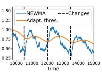
The two strategies presented above are generally difficult to carry out in practice, since we do not know the in-control distribution π𝜋\pi. If we had access to training data, a classical method would be to estimate either the ARL or the distribution of St=def.𝐳t𝐳tsuperscriptdef.subscript𝑆𝑡normsubscriptsuperscript𝐳𝑡subscript𝐳𝑡S_{t}\stackrel{{\scriptstyle\textrm{{def.}}}}{{=}}\left\|\mathbf{z}^{\prime}_{t}-\mathbf{z}_{t}\right\| during a “Phase 1” estimation, before the actual run. In the case where we do not have access to training data beforehand, we propose to adapt the second strategy and perform an online estimation of the distribution of the statistic Stsubscript𝑆𝑡S_{t}, which yields a dynamic threshold τtsubscript𝜏𝑡\tau_{t} that can adapt to multiple changes in a continuous run (Fig. 8).

According to Thm. 5, St2superscriptsubscript𝑆𝑡2S_{t}^{2} asymptotically follows a distribution formed by a linear combination of an infinite number of independent centered normalized Gaussians with unknown weights ξsubscript𝜉\xi_{\ell}. While it would be possible to estimate these weights with relatively heavy computations by maintaining a Gram matrix [21], in the spirit of the paper we propose a light method that assume that St2superscriptsubscript𝑆𝑡2S_{t}^{2} itself is approximately Gaussian: indeed, it is easy to see that with additional assumptions on the ξsubscript𝜉\xi_{\ell}, generalizations of the Central Limit Theorem (see e.g. Th. 12) would guarantee that with proper normalization the r.h.s. of (7) converges to a Gaussian (details are omitted here).

Hence, if we consider St2superscriptsubscript𝑆𝑡2S_{t}^{2} to be Gaussian, we just need to estimate its mean μtsubscript𝜇𝑡\mu_{t} and standard deviation σtsubscript𝜎𝑡\sigma_{t}, which we do with a simple online estimation procedure using exponential weights with a learning rate α𝛼\alpha (Alg. 7), to continuously adapt in the case of multiple changes. Then the threshold at time t𝑡t is set as τt2=μt+aσtsuperscriptsubscript𝜏𝑡2subscript𝜇𝑡𝑎subscript𝜎𝑡\tau_{t}^{2}=\mu_{t}+a\sigma_{t}, where a𝑎a is chosen according to the desired quantile of the normal distribution (e.g., a=1.64𝑎1.64a=1.64 for 5%percent55\% of false alarms). Recall that the amplitude of a change between π𝜋\pi and πsuperscript𝜋\pi^{\prime} is approximately described by (3) (and (5) when using RFs), and that we can expect a successful detection when it is higher than the threshold.

While this method relies on a heuristic than may not necessarily be satisfied, we found in practice this adaptive procedure to perform better than any fixed threshold, while avoiding having to set it. In our experiments, we applied the same strategy to other change-point detection algorithms that produce positive statistics Stsubscript𝑆𝑡S_{t} such as SW or Scan-B𝐵B, and found the procedure to perform extremely well in each case. We leave its theoretical analysis for future work, and emphasize again that, in case where training data is available, more complex or computationally intensive procedures could be used.
Refer to caption
Figure 8: Illustration of the adaptive threshold procedure. The dotted line indicate a change, the blue line is the NEWMA statistic 𝐳t𝐳tnormsubscript𝐳𝑡subscriptsuperscript𝐳𝑡\left\|\mathbf{z}_{t}-\mathbf{z}^{\prime}_{t}\right\|, and in yellow line is the adaptive threshold computed online as described in Sec. 5.3.

6 Experiments

In this experimental section we compare several model-free approaches: NEWMA where ΨΨ\Psi is one of the three different random features schemes described in Sec. 4: classical RFFs [36], FF [29], or OPU [38], the SW algorithm (Alg. 2[3]) with RFFs, and the kernel Scan-B𝐵B algorithm [30] with N=3𝑁3N=3 windows. Scan-B𝐵B is implemented with a Gaussian kernel κ(x,x)=exx22σ2𝜅𝑥superscript𝑥superscript𝑒superscriptnorm𝑥superscript𝑥22superscript𝜎2\kappa(x,x^{\prime})=e^{-\frac{\left\|x-x^{\prime}\right\|^{2}}{2\sigma^{2}}} with a bandwidth σ𝜎\sigma chosen by the median trick. All other methods use RFs that correspond to the same kernel, either complex exponentials for RFFs (see Section 4.3) or the Fastfood (FF) method [29], except when using the OPU, for which the RFs and corresponding kernel are imposed by the optical hardware [38].

Remark 3.

We do not compare NEWMA with parametric methods such as GLR or CUSUM, or methods requiring prior knowledge such as EWMA, since the settings are very different and fair comparison would be difficult. In the presence of parametric modelling assumptions or prior knowledge, we naturally expect the algorithms exploiting them to perform better than model-free methods such as SW, Scan-B𝐵B or NEWMA.

The experiments run on a laptop with an Intel Xeon Gold 6128 3.40GHz. The code is available at https://github.com/lightonai/newma.
Refer to caption
Refer to caption
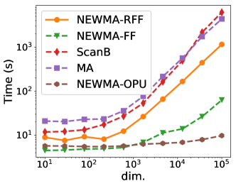
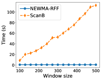
Figure 9: Time of execution on 120001200012000 samples with m=3000𝑚3000m=3000 RFs for NEWMA and SW, window size B=250𝐵250B=250 for Scan-B𝐵B and SW, and dimension d=100𝑑100d=100 unless otherwise precised.
Refer to caption
Refer to caption
(a) Number of random features m𝑚m.
Refer to caption
Refer to caption
(b) Choice of σ𝜎\sigma for Gaussian kernel.
Refer to caption
Refer to caption
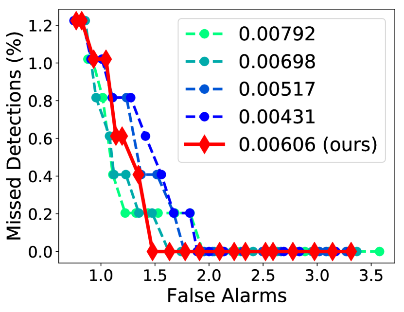
(c) Choice of ΛΛ\Lambda, for a fixed window size B𝐵B (for λ=λΛ,B𝜆subscript𝜆Λ𝐵\lambda=\lambda_{\Lambda,B}).
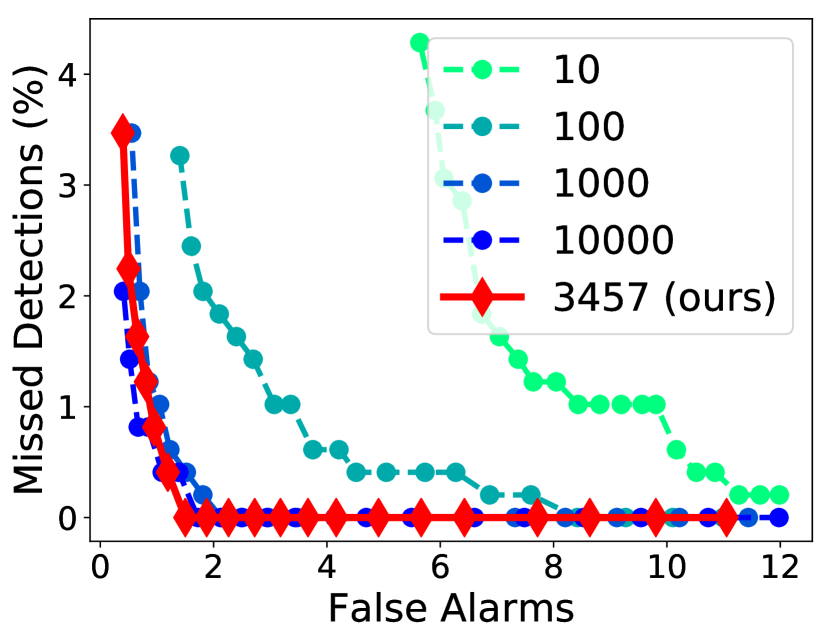
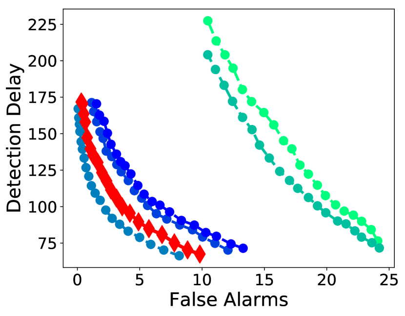
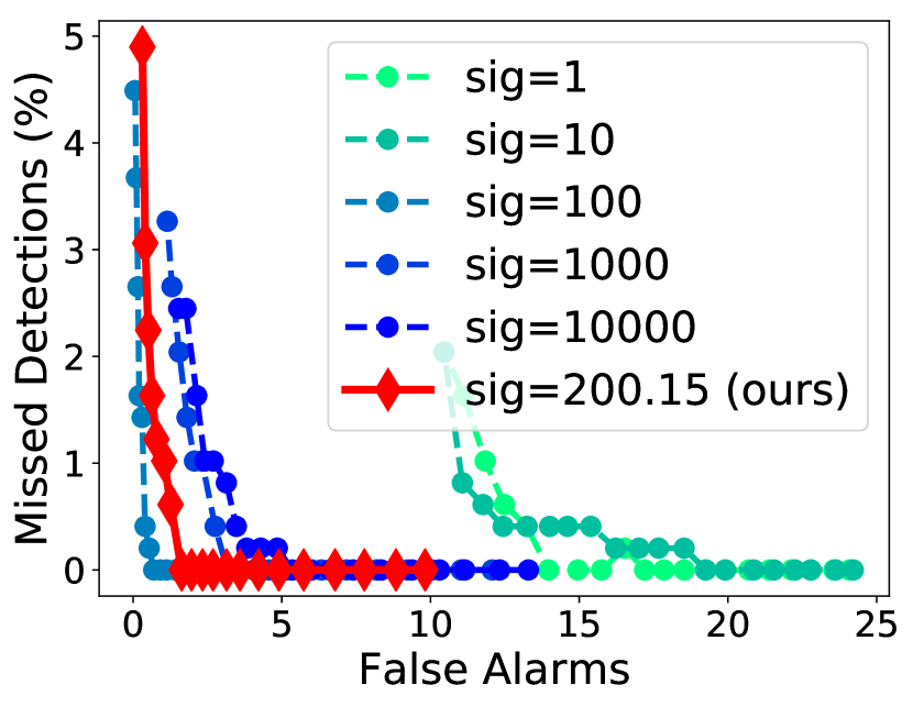
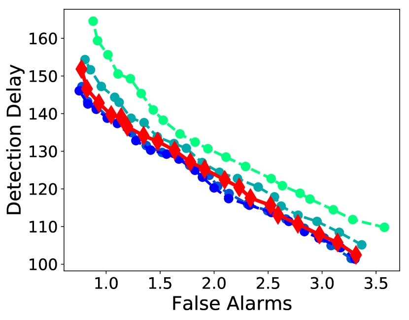
Figure 10: Effect of the choice of hyperparameters in NEWMA. The thick red line indicates the proposed choices.
Refer to caption
Refer to caption
(a) Synthetic data.
Refer to caption
Refer to caption
(b) Audio data.
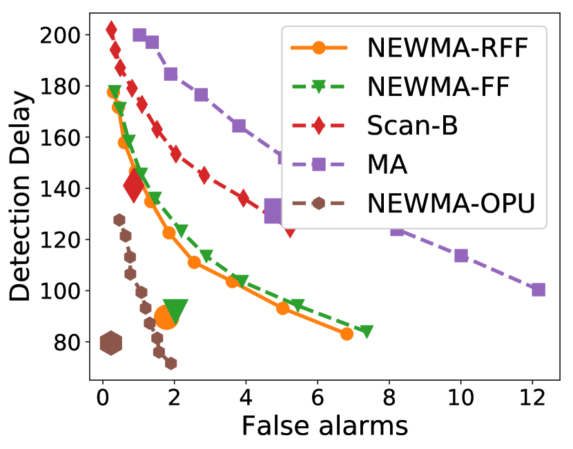
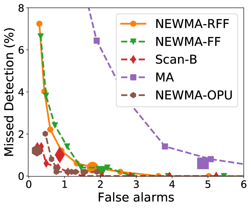
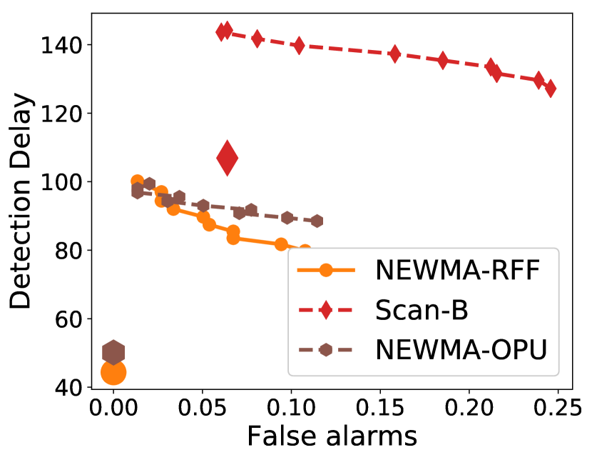
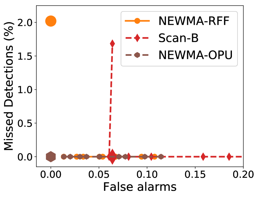
Figure 11: Experimental results. The solid lines corresponds to several possible choices of a fixed threshold τ𝜏\tau, while the single large dot corresponds to the performance of the adaptive threshold procedure described in Sec. 5.3.

6.1 Time of execution

In Fig. 9 we examine the time of execution of the algorithms with respect to the dimension d𝑑d of the data and window size B𝐵B. Being similar, Scan-B𝐵B and SW have approximately the same running time. As expected, NEWMA-FF is sublinear in the dimension, and NEWMA-OPU is almost independent of the dimension and much faster than the other approaches in high dimension. The results also confirm that NEWMA’s complexity is independent of B𝐵B, while that of Scan-B𝐵B increases linearly with B𝐵B.

6.2 Comparison of algorithms on synthetic data

Next we examine the detection performance of the algorithms on synthetic data. We generate the data as follows: 106superscript10610^{6} samples are drawn from Gaussian Mixture Models (GMM) in dimension d=100𝑑100d=100 with k=10𝑘10k=10 components, and the GMM changes every n=2000𝑛2000n=2000 samples (at each change, we draw k𝑘k new vector means according to a centered Gaussian distribution, k𝑘k new covariance matrices from an inverse-Wishart distribution, and k𝑘k new mixing weights from a Dirichlet distribution), resulting in 500 changes to detect in a row. We recall that these settings are more typical of online methods, where changes are detected on-the-fly, rather than offline ones, for which a high number of changes results in a high computational complexity and memory-load. Note that the considered changes are rather complex, with high-dimensional, multimodal, unknown distributions before and after the change, so that classical parametric change-point detection methods cannot be applied here. For all algorithms we use a window size B=250𝐵250B=250.

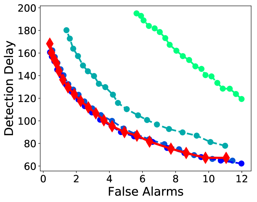
To evaluate performance we compute false alarm rate, missed detections, and detection delay. We consider that the algorithm should be stable before every true change and we count every detected change in the n/2 samples before it as a false alarm. We record the time until the first detected change in the n/2 samples after every true change as detection delay, and we record a missed detection if no change is detected. This is then repeated for 500 changes in a row, and all statistics are averaged by the number of changes. We plot different ratios Expected Detection Delay (EDD)-to-Number of False Alarms or Missed Detections-to-Number of False Alarms (lower left corner is better), by varying a fixed threshold τ𝜏\tau. In Fig. 11, the result of the adaptive threshold procedure of Sec. 5.3 is plotted as single large dots.

Effects of the hyperparameters

In Fig. 10, we examine the effects of the different hyperparameters in NEWMA and our choices described in the previous sections.

In Fig. 10(a), we set the forgetting factors ΛsuperscriptΛ\Lambda^{\star} and λsuperscript𝜆\lambda^{\star} according to Sec. 3.3, and vary the number of random features m𝑚m. We compare it with our prescribed choice from Prop. 3, m=𝒪((Λ+λ)2)superscript𝑚𝒪superscriptsuperscriptΛsuperscript𝜆2m^{\star}=\mathcal{O}\left((\Lambda^{\star}+\lambda^{\star})^{-2}\right) (in practice we choose an arbitrary multiplicative constant 1/4141/4 to reduce computation time). As expected, the performance of the detection increases with m𝑚m, and at low m𝑚m the algorithm is observed to be relatively unstable. However, it is also seen that increasing m𝑚m beyond our choice msuperscript𝑚m^{\star} has negligible effect, so that our heuristic seems to yield the right order of magnitude for m𝑚m. In the rest of the experiments we always choose m=14(Λ+λ)2𝑚14superscriptsuperscriptΛsuperscript𝜆2m=\frac{1}{4}(\Lambda^{\star}+\lambda^{\star})^{-2}, except when using the OPU, for which we choose 101010 times this value since we do not have computational restrictions in this case.

In Fig. 10(b) we examine the choice of the kernel bandwidth σ𝜎\sigma, and compare different values with the median trick that we use in practice. It is seen that the median trick yields a correct order of magnitude of about 102superscript10210^{2}, with all other values performing worse.

Finally, in Fig. 10(c) we vary the forgetting factor ΛΛ\Lambda, while keeping the window size B𝐵B constant by choosing λ=λΛ,B𝜆subscript𝜆Λ𝐵\lambda=\lambda_{\Lambda,B}. It is seen that our prescribed choice (Λ,λ)superscriptΛsuperscript𝜆(\Lambda^{\star},\lambda^{\star}) offers a balanced performance: increasing ΛΛ\Lambda worsens the number of missed detections while only marginally decreasing the detection delay, and decreasing ΛΛ\Lambda has the inverse effect.

Comparison of algorithms

In Fig. 11(a) we compare the algorithms on synthetic data. We first observe that the adaptive threshold procedure, indicated by single large dots in the figure, is consistently better than any fixed threshold for all algorithms.

It is seen that SW performs generally poorly, confirming the superiority of Scan-B𝐵B as a window-based approach. NEWMA with Gaussian random features (RFF or FF) exhibits a reduced detection delay compared to Scan-B𝐵B but a slightly higher number of missed detections. NEWMA-OPU is seen to perform well, which may indicate that the kernel induced by the OPU is more appropriate than a Gaussian kernel on this example.

6.3 Real Data: voice activity detection

We apply our method to a Voice Activity Detection (VAD) task on audio data. We consider real environments background noise from the QUT-NOISE dataset [14] and add, every 101010s, a 333s speech extract from the TIMIT dataset [18], with 7.57.5-7.5dB Signal-to-Noise Ratio. Our goal is to detect the onset of the speech segments. We use the Short Time Fourier Transform (STFT) of the signal, a Fourier transform localized in time that is ubiquitous in audio and speech processing [12]. It allows to extract on-the-fly frequency information from the one-dimensional audio signal stsubscript𝑠𝑡s_{t}, turning it into a d=128𝑑128d=128-dimensional time series xtdsubscript𝑥𝑡superscript𝑑x_{t}\in\mathbb{R}^{d}, where d𝑑d is the number of considered frequencies (usually the time axis is also dilated between stsubscript𝑠𝑡s_{t} and xtsubscript𝑥𝑡x_{t}). For xtsubscript𝑥𝑡x_{t}, we consider a change every 125012501250 samples, and 300300300 changes in total. We take a window size B=150𝐵150B=150. We display the results in Fig. 11(b). Similar to the results on synthetic data, Scan-B𝐵B has a higher detection delay than NEWMA. However, it does also exhibit slightly more missed detections: we suspect that, because it uses several windows of reference in-control samples, Scan-B𝐵B is sensitive to highly heterogeneous data, which can be the case for audio data. In this case, the Gaussian random features are seen to perform on par with the OPU kernel.

7 Conclusion and outlooks

We introduced NEWMA, a new method for online change-point detection that is faster and lighter than existing model-free methods. The simple, key idea behind NEWMA is to compare recursive averages computed with different forgetting factors on the same data, in order to extract time-varying information without keeping in memory the raw data.

In the future, we plan to further develop the analysis of our method under the null to derive properties that do not depend on the in-control distribution, as done in [30]. Additionally, the robustness of the random generalized moments methodology to noise and missing data appears as an interesting extension. Recent approaches for learning from random feature moments [23] would allow extracting more information from 𝐳t𝐳tsubscript𝐳𝑡subscriptsuperscript𝐳𝑡\mathbf{z}_{t}-\mathbf{z}^{\prime}_{t} than mere occurence of a change, without increasing the computational load. Another direction for our research is the study of mappings ΨΨ\Psi for graph data, which, combined with NEWMA, would allow to detect changes in large-scale social networks [34].

Acknowledgment

The authors would like to thank LightOn for the use of the OPU, Francis Bach and Sylvain Arlot for discussions on the idea behind NEWMA.

References

  • [1] A. Abou-Elailah, V. Gouet-Brunet, and I. Bloch. Detection of abrupt changes in spatial relationships in video sequences. In International Conference on Pattern Recognition Applications and Methods, pages 89–106. Springer, 2015.
  • [2] Stephanie Allen, David Madras, and Ye Ye. Change-point Detection Methods for Body-Worn Video. arXiv:1610.06453, 2016.
  • [3] Shai Ben-David, Johannes Gehrke, and Daniel Kifer. Detecting Change in Data Streams. Proceedings of the 30th VLDB Conference, pages 180–191, 2004.
  • [4] C. Berg, J. Christensen, and P. Ressel. Harmonic analysis on semigroups. 100, 1984.
  • [5] Alain Berlinet and Christine Thomas-Agnan. Reproducing Kernel Hilbert Spaces in Probability and Statistics. Kluwer Academics Publisher, 2004.
  • [6] A. Bietti, F. Bach, and A. Cont. An online em algorithm in hidden (semi-) markov models for audio segmentation and clustering. In Acoustics, Speech and Signal Processing (ICASSP), pages 1881–1885. IEEE, 2015.
  • [7] Marcel Bosc, Fabrice Heitz, Jean Paul Armspach, Izzie Namer, Daniel Gounot, and Lucien Rumbach. Automatic change detection in multimodal serial mri: application to multiple sclerosis lesion evolution. NeuroImage, 20 2:643–56, 2003.
  • [8] Stéphane Boucheron, Gábor Lugosi, and Pascal Massart. Concentration inequalities: A nonasymptotic theory of independence. Oxford University Press, 2013.
  • [9] Kevin C. Cheng, Shuchin Aeron, Michael C. Hughes, Erika Hussey, and Eric L. Miller. Optimal Transport Based Change Point Detection and Time Series Segment Clustering. 2019.
  • [10] Kacper Chwialkowski, Aaditya Ramdas, Dino Sejdinovic, and Arthur Gretton. Fast Two-Sample Testing with Analytic Representations of Probability Measures. In Advances in Neural Information Processing Systems (NIPS), 2015.
  • [11] Petar Čisar and Sanja Maravić Čisar. Optimization methods of EWMA statistics. Acta Polytechnica Hungarica, 8(5):73–87, 2011.
  • [12] Leon Cohen. Time-Frequency Analysis. Prentice-Hall, PTR, 1995.
  • [13] A. F. B. Costa and M. A. Rahim. A Single EWMA Chart for Monitoring Process Mean and Process Variance. Quality Technology and Quantitative Management, 3(3):295–305, 2006.
  • [14] David Dean, Sridha Sridharan, Robert Vogt, and Michael Mason. The QUT-NOISE-TIMIT corpus for the evaluation of voice activity detection algorithms. In Proceedings of Interspeech, number September, pages 26–30, 2010.
  • [15] Angélique Drémeau, Antoine Liutkus, David Martina, Ori Katz, Christophe Schülke, Florent Krzakala, Sylvain Gigan, and Laurent Daudet. Reference-less measurement of the transmission matrix of a highly scattering material using a DMD and phase retrieval techniques. Optics Express, 23(9):11898, 2015.
  • [16] Deena P Francis and Kumudha Raimond. A Random Fourier Features based Streaming Algorithm for Anomaly Detection in Large Datasets, volume 645. Springer Singapore, 2018.
  • [17] James C Fu, Fred A. Spiring, and Hansheng Xie. On the average run length of quality control schemes using a Markov Chain approach. Statistics & Probability Letters, 56(4):369–380, 2002.
  • [18] John S. Garofolo, Lori F. Lamel, William M. Fisher, Jonathan G. Fiscus, David S. Pallett, Nancy L. Dahlgren, and Victor Zue. TIMIT Acoustic-Phonetic Continuous Speech Corpus LDC93S1, 1993.
  • [19] Damien Garreau and Sylvain Arlot. Consistent change-point detection with kernels. Electronic Journal of Statistics, 12(2):4440–4486, 2018.
  • [20] Parikshit Gopalan, Vatsal Sharan, and Udi Wieder. Faster Anomaly Detection via Matrix Sketching. (Nips), 2018.
  • [21] A. Gretton, K. Fukumizu, Z. Harchaoui, and B. K. Sriperumbudur. A Fast, Consistent Kernel Two-Sample Test. In Advances in Neural Information Processing Systems (NIPS), pages 673–681, 2009.
  • [22] Arthur Gretton, Karsten M. Borgwardt, Malte J. Rasch, Bernhard Schölkopf, and Alexander J. Smola. A Kernel Method for the Two-Sample Problem. In Advances in Neural Information Processing Systems (NIPS), pages 513–520, 2007.
  • [23] Rémi Gribonval, Gilles Blanchard, Nicolas Keriven, and Yann Traonmilin. Compressive Statistical Learning with Random Feature Moments. arXiv:1706.07180, pages 1–72, 2017.
  • [24] D. Han, F. Tsung, X. Hu, and K. Wang. CUSUM and EWMA multi-charts for detecting a range of mean shifts. Statistica Sinica, 17(3):1139–1164, 2007.
  • [25] Zaïd Harchaoui, Francis Bach, and Eric Moulines. Kernel change-point analysis. In Advances in Neural Information Processing Systems (NIPS), pages 609–616, 2009.
  • [26] D. Hawkins and Qiqi Deng. A Nonparametric Change-Point Control Chart. Journal of Quality Technology, 42(2):165–173, 2010.
  • [27] Naveed Khan, Sally McClean, Shuai Zhang, and Chris Nugent. Optimal Parameter Exploration for Online Change-Point Detection in Activity Monitoring Using Genetic Algorithms. Sensors, 16(11), 2016.
  • [28] Albert Y. Kim, C. Marzban, D. Percival, and W. Stuetzle. Using labeled data to evaluate change detectors in a multivariate streaming environment. Signal Processing, 89(12):2529–2536, 2009.
  • [29] Quoc V Le, Tamás Sarlós, and Alexander J. Smola. Fastfood - Approximating Kernel Expansions in Loglinear Time. In International Conference on Machine Learning (ICML), volume 28, 2013.
  • [30] Shuang Li, Yao Xie, Hanjun Dai, and Le Song. Scan B-Statistic for Kernel Change-Point Detection. arXiv:1507.01279, pages 1–48, 2015.
  • [31] Song Liu, Makoto Yamada, Nigel Collier, and Masashi Sugiyama. Change-point detection in time-series data by relative density-ratio estimation. Neural Networks, 43:72–83, 2013.
  • [32] CA A Lowry and WH H Woodall. A multivariate exponentially weighted moving average control chart. Technometrics, 34(1):46–53, 1992.
  • [33] R. Malladi, G. P. Kalamangalam, and B. Aazhang. Online bayesian change point detection algorithms for segmentation of epileptic activity. In Asilomar Conference on Signals, Systems and Computers, pages 1833–1837, Nov 2013.
  • [34] Leto Peel and Aaron Clauset. Detecting change points in the large-scale structure of evolving networks. In AAAI Conference on Artificial Intelligence, pages 1–11, 2015.
  • [35] A. Polunchenko and A. Tartakovsky. State-of-the-art in sequential change-point detection. Methodology and computing in applied probability, 14(3):649–684, 2012.
  • [36] Ali Rahimi and Benjamin Recht. Random Features for Large Scale Kernel Machines. In Advances in Neural Information Processing Systems (NIPS), 2007.
  • [37] S. W. Roberts. Control Chart Tests Based on Geometric Moving Averages. Technometrics, 1(3):239–250, 1959.
  • [38] Alaa Saade, Francesco Caltagirone, Igor Carron, Laurent Daudet, Angélique Dremeau, Sylvain Gigan, and Florent Krzakala. Random projections through multiple optical scattering: Approximating Kernels at the speed of light. In IEEE International Conference on Acoustic, Speech and Signal Processing (ICASSP), pages 6215–6219, 2016.
  • [39] Robert J Serfling. Approximation Theorems of Mathematical Statistics, volume 37. John Wiley & Sons, Inc., 1980.
  • [40] Bharath K. Sriperumbudur, Arthur Gretton, Kenji Fukumizu, Bernhard Schölkopf, and Gert R.G. Lanckriet. Hilbert space embeddings and metrics on probability measures. The Journal of Machine Learning Research, 11:1517–1561, 2010.
  • [41] M. Staudacher, S. Telser, A. Amann, H. Hinterhuber, and M. Ritsch-Marte. A new method for change-point detection developed for on-line analysis of the heart beat variability during sleep. Physica A: Statistical Mechanics and its Applications, 349(3):582 – 596, 2005.
  • [42] Dougal J. Sutherland, Junier B. Oliva, Poczos Barnabas, and Jeff Schneider. Linear-time Learning on Distributions with Approximate Kernel Embeddings. arXiv:1509.07553, 2015.
  • [43] A W van der Vaart. Asymptotic Statistics. Cambridge University Press, 1998.
  • [44] Jonathan Weed and Francis Bach. Sharp asymptotic and finite-sample rates of convergence of empirical measures in Wasserstein distance. pages 1–35, 2017.
  • [45] Yao Xie, Meng Wang, and Andrew Thompson. Sketching for sequential change-point detection. 2015 IEEE Global Conference on Signal and Information Processing, GlobalSIP 2015, pages 78–82, 2016.
  • [46] T Yang, M Mahdavi, R Jin, J Yi, and Sch Hoi. Online Kernel Selection: Algorithms and Evaluations. In AAAI Conference on Artifical Intelligence, pages 1197–1203, 2012.
  • [47] Changliang Zou and Fugee Tsung. Likelihood Ratio-Based Distribution-Free EWMA Control Charts. Journal of Quality Technology, 42(2):1–23, 2010.

Appendix A Proofs of theorems 4 and 5

We start with some elementary computations that are used throughout the rest of the proofs. Set 0<λ<Λ<10𝜆Λ10<\lambda<\Lambda<1. For t1𝑡1t\geq 1 and it𝑖𝑡i\leq t, define α0=(1Λ)tsubscript𝛼0superscript1Λ𝑡\alpha_{0}=(1-\Lambda)^{t}, β0=(1λ)tsubscript𝛽0superscript1𝜆𝑡\beta_{0}=(1-\lambda)^{t}, αi=Λ(1Λ)tiandβi=λ(1λ)tiformulae-sequencesubscript𝛼𝑖Λsuperscript1Λ𝑡𝑖andsubscript𝛽𝑖𝜆superscript1𝜆𝑡𝑖\alpha_{i}=\Lambda(1-\Lambda)^{t-i}\quad\text{and}\quad\beta_{i}=\lambda(1-\lambda)^{t-i}, such that in NEWMA 𝐳t=α0𝐳0+i=1tαiΨ(xi)subscript𝐳𝑡subscript𝛼0subscript𝐳0superscriptsubscript𝑖1𝑡subscript𝛼𝑖Ψsubscript𝑥𝑖\mathbf{z}_{t}=\alpha_{0}\mathbf{z}_{0}+\sum_{i=1}^{t}\alpha_{i}\Psi\left(x_{i}\right) and similarly for 𝐳tsubscriptsuperscript𝐳𝑡\mathbf{z}^{\prime}_{t} and βisubscript𝛽𝑖\beta_{i}. Then, for any 1t1<t2t1subscript𝑡1subscript𝑡2𝑡1\leq t_{1}<t_{2}\leq t, we have

i=0t1αisuperscriptsubscript𝑖0subscript𝑡1subscript𝛼𝑖\displaystyle\sum_{i=0}^{t_{1}}\alpha_{i} =(1Λ)tt1,absentsuperscript1Λ𝑡subscript𝑡1\displaystyle=(1-\Lambda)^{t-t_{1}}, (8)
i=t1t2αisuperscriptsubscript𝑖subscript𝑡1subscript𝑡2subscript𝛼𝑖\displaystyle\sum_{i=t_{1}}^{t_{2}}\alpha_{i} =(1Λ)tt2(1Λ)tt1+1absentsuperscript1Λ𝑡subscript𝑡2superscript1Λ𝑡subscript𝑡11\displaystyle=(1-\Lambda)^{t-t_{2}}-(1-\Lambda)^{t-t_{1}+1} (9)

and similarly for β𝛽\beta with λ𝜆\lambda, and

i=1tαir1βir2superscriptsubscript𝑖1𝑡superscriptsubscript𝛼𝑖subscript𝑟1superscriptsubscript𝛽𝑖subscript𝑟2\displaystyle\sum_{i=1}^{t}\alpha_{i}^{r_{1}}\beta_{i}^{r_{2}} =Λr1λr2(1At)1A, with A=(1Λ)r1(1λ)r2.formulae-sequenceabsentsuperscriptΛsubscript𝑟1superscript𝜆subscript𝑟21superscript𝐴𝑡1𝐴 with 𝐴superscript1Λsubscript𝑟1superscript1𝜆subscript𝑟2\displaystyle=\tfrac{\Lambda^{r_{1}}\lambda^{r_{2}}(1-A^{t})}{1-A},\text{ with }A=(1-\Lambda)^{r_{1}}(1-\lambda)^{r_{2}}\,. (10)

A.1 Mean time between false alarm (Thm. 4)

In this section, we prove a multi-dimensional generalization of Theorem 4 (Theorem 6), inspired by the approach in [17].

Assuming all samples xtsubscript𝑥𝑡x_{t} are drawn i.i.d. from a distribution π𝜋\pi, recall that we define the ARL under control as

T¯=𝔼[inf{t|Stτ}].¯𝑇𝔼delimited-[]infimumconditional-set𝑡subscript𝑆𝑡𝜏\overline{T}=\mathbb{E}\left[\inf\left\{t~{}|~{}S_{t}\geq\tau\right\}\right]\,. (11)

where in the case of NEWMA, we have St=𝐳t𝐳tsubscript𝑆𝑡normsubscript𝐳𝑡subscriptsuperscript𝐳𝑡S_{t}=\left\|\mathbf{z}_{t}-\mathbf{z}^{\prime}_{t}\right\|. In this section, we derive a more tractable expression for T¯¯𝑇\overline{T}.

Our proof strategy relies on the observation that (𝐳t,𝐳t)subscript𝐳𝑡subscriptsuperscript𝐳𝑡(\mathbf{z}_{t},\mathbf{z}^{\prime}_{t}) is a Markov chain in 2superscript2\mathcal{H}^{2}, and thus it is possible to apply a method similar to [17] for classical EWMA, with non-trivial modifications. We assume here that =def.msuperscriptdef.superscript𝑚\mathcal{H}\stackrel{{\scriptstyle\textrm{{def.}}}}{{=}}\mathbb{R}^{m}, that is, Ψ:dm:Ψsuperscript𝑑superscript𝑚\Psi:\mathbb{R}^{d}\to\mathbb{R}^{m}. Since the stopping condition for NEWMA involves both components 𝐳tsubscript𝐳𝑡\mathbf{z}_{t} and 𝐳tsubscriptsuperscript𝐳𝑡\mathbf{z}^{\prime}_{t} of the chain, we define the set Vτ2subscript𝑉𝜏superscript2V_{\tau}\subset\mathcal{H}^{2} as the domain in which the algorithm continues:

Vτ=def.{𝐯=(𝐳,𝐳)|𝐳𝐳<τ}.superscriptdef.subscript𝑉𝜏conditional-set𝐯𝐳superscript𝐳norm𝐳superscript𝐳𝜏V_{\tau}\stackrel{{\scriptstyle\textrm{{def.}}}}{{=}}\left\{\mathbf{v}=(\mathbf{z},\mathbf{z}^{\prime})~{}|~{}\left\|\mathbf{z}-\mathbf{z}^{\prime}\right\|<\tau\right\}\,. (12)

With these notations, when we run NEWMA and stop as soon as an alarm is raised, we produce a Markov chain 𝐯t2subscript𝐯𝑡superscript2\mathbf{v}_{t}\in\mathcal{H}^{2} defined as: 𝐯0=(𝐳0,𝐳0)subscript𝐯0subscript𝐳0subscript𝐳0\mathbf{v}_{0}=(\mathbf{z}_{0},\mathbf{z}_{0}), and

𝐯t={((1Λ)𝐯t1,1+ΛΨ(xt)(1λ)𝐯t1,2+λΨ(xt)) if 𝐯t1Vτ,𝐯t1 otherwise.subscript𝐯𝑡casesmatrix1Λsubscript𝐯𝑡11ΛΨsubscript𝑥𝑡1𝜆subscript𝐯𝑡12𝜆Ψsubscript𝑥𝑡 if subscript𝐯𝑡1subscript𝑉𝜏subscript𝐯𝑡1 otherwise.\mathbf{v}_{t}=\begin{cases}\left(\begin{matrix}(1-\Lambda)\mathbf{v}_{t-1,1}+\Lambda\Psi\left(x_{t}\right)\\ (1-\lambda)\mathbf{v}_{t-1,2}+\lambda\Psi\left(x_{t}\right)\end{matrix}\right)&\text{ if }\mathbf{v}_{t-1}\in V_{\tau}\,,\\ \mathbf{v}_{t-1}&\text{ otherwise.}\end{cases}

In other words, the chain is stationary as soon as an alarm is raised. In order to state our theorem, we need to introduce a fair amount of notations. Consider the space 2=×superscript2\mathcal{H}^{2}=\mathcal{H}\times\mathcal{H}, equipped with the norm (𝐱,𝐱)=𝐱+𝐱norm𝐱superscript𝐱norm𝐱normsuperscript𝐱\left\|(\mathbf{x},\mathbf{x}^{\prime})\right\|=\left\|\mathbf{x}\right\|+\left\|\mathbf{x}^{\prime}\right\|. For ε>0𝜀0\varepsilon>0, consider the ball of radius ε1superscript𝜀1\varepsilon^{-1} in 2superscript2\mathcal{H}^{2}, ε={𝐯|𝐯1/ε}subscript𝜀conditional-set𝐯norm𝐯1𝜀\mathcal{B}_{\varepsilon}=\left\{\mathbf{v}~{}|~{}\left\|\mathbf{v}\right\|\leq 1/\varepsilon\right\}, which is compact since 2superscript2\mathcal{H}^{2} has finite dimension. Define 𝒞ε={𝐮1,,𝐮Nε}εsubscript𝒞𝜀subscript𝐮1subscript𝐮subscript𝑁𝜀subscript𝜀\mathcal{C}_{\varepsilon}=\left\{\mathbf{u}_{1},\ldots,\mathbf{u}_{N_{\varepsilon}}\right\}\subset\mathcal{B}_{\varepsilon} any ε𝜀\varepsilon-net of εsubscript𝜀\mathcal{B}_{\varepsilon} (we will see that its choice does not matter) such that 𝐮1=(𝐳0,𝐳0)subscript𝐮1subscript𝐳0subscript𝐳0\mathbf{u}_{1}=(\mathbf{z}_{0},\mathbf{z}_{0}), where Nεsubscript𝑁𝜀N_{\varepsilon} is the ε𝜀\varepsilon-covering number of εsubscript𝜀\mathcal{B}_{\varepsilon}. Without lost of generality, assume they are ordered such that 𝐮1,𝐮MεVτsubscript𝐮1subscript𝐮subscript𝑀𝜀subscript𝑉𝜏\mathbf{u}_{1},\ldots\mathbf{u}_{M_{\varepsilon}}\in V_{\tau} and 𝐮Mε+1,,𝐮NεVτcsubscript𝐮subscript𝑀𝜀1subscript𝐮subscript𝑁𝜀superscriptsubscript𝑉𝜏𝑐\mathbf{u}_{M_{\varepsilon}+1},\ldots,\mathbf{u}_{N_{\varepsilon}}\in V_{\tau}^{c} for some Mεsubscript𝑀𝜀M_{\varepsilon}. Denote Pε:2𝒞ε:subscript𝑃𝜀superscript2subscript𝒞𝜀P_{\varepsilon}:\mathcal{H}^{2}\to\mathcal{C}_{\varepsilon} the projection operator onto 𝒞εsubscript𝒞𝜀\mathcal{C}_{\varepsilon} (i.e., that returns the 𝐮isubscript𝐮𝑖\mathbf{u}_{i} closest to its input). Define the following Markov chain 𝐯tε𝒞εsuperscriptsubscript𝐯𝑡𝜀subscript𝒞𝜀\mathbf{v}_{t}^{\varepsilon}\in\mathcal{C}_{\varepsilon}: initialize 𝐯0ε=(𝐳0,𝐳0)=𝐮1superscriptsubscript𝐯0𝜀subscript𝐳0subscript𝐳0subscript𝐮1\mathbf{v}_{0}^{\varepsilon}=(\mathbf{z}_{0},\mathbf{z}_{0})=\mathbf{u}_{1}, and

𝐯tε={Pε(((1Λ)𝐯t1,1ε+ΛΨ(xt)(1λ)𝐯t1,2ε+λΨ(xt))) if 𝐯t1εVτ,𝐯t1ε otherwise.superscriptsubscript𝐯𝑡𝜀casessubscript𝑃𝜀matrix1Λsuperscriptsubscript𝐯𝑡11𝜀ΛΨsubscript𝑥𝑡1𝜆superscriptsubscript𝐯𝑡12𝜀𝜆Ψsubscript𝑥𝑡 if superscriptsubscript𝐯𝑡1𝜀subscript𝑉𝜏superscriptsubscript𝐯𝑡1𝜀 otherwise.\mathbf{v}_{t}^{\varepsilon}=\begin{cases}P_{\varepsilon}\left(\left(\begin{matrix}(1-\Lambda)\mathbf{v}_{t-1,1}^{\varepsilon}+\Lambda\Psi\left(x_{t}\right)\\ (1-\lambda)\mathbf{v}_{t-1,2}^{\varepsilon}+\lambda\Psi\left(x_{t}\right)\end{matrix}\right)\right)&\text{ if }\mathbf{v}_{t-1}^{\varepsilon}\in V_{\tau}\,,\\ \mathbf{v}_{t-1}^{\varepsilon}&\text{ otherwise.}\end{cases}

It is a projected and bounded version of the output of NEWMA, which is stationary as soon as it gets out of Vτsubscript𝑉𝜏V_{\tau}. Finally, for 1i,jNεformulae-sequence1𝑖𝑗subscript𝑁𝜀1\leq i,j\leq N_{\varepsilon}, define pij=(𝐯t+1ε=𝐮j|𝐯tε=𝐮i)subscript𝑝𝑖𝑗superscriptsubscript𝐯𝑡1𝜀conditionalsubscript𝐮𝑗superscriptsubscript𝐯𝑡𝜀subscript𝐮𝑖p_{ij}=\mathbb{P}\left(\mathbf{v}_{t+1}^{\varepsilon}=\mathbf{u}_{j}~{}|~{}\mathbf{v}_{t}^{\varepsilon}=\mathbf{u}_{i}\right) the transition probabilities of the markov chain 𝐯tεsuperscriptsubscript𝐯𝑡𝜀\mathbf{v}_{t}^{\varepsilon}. Define 𝐀=[pij]1i,jMε𝐀subscriptdelimited-[]subscript𝑝𝑖𝑗formulae-sequence1𝑖𝑗subscript𝑀𝜀\mathbf{A}=\left[p_{ij}\right]_{1\leq i,j\leq M_{\varepsilon}} that corresponds to the states 𝐮iVτsubscript𝐮𝑖subscript𝑉𝜏\mathbf{u}_{i}\in V_{\tau}, all other states being absorbant, and aij()superscriptsubscript𝑎𝑖𝑗a_{ij}^{(\ell)} such that 𝐀=[aij()]1i,jMεsuperscript𝐀subscriptdelimited-[]superscriptsubscript𝑎𝑖𝑗formulae-sequence1𝑖𝑗subscript𝑀𝜀\mathbf{A}^{\ell}=\left[a_{ij}^{(\ell)}\right]_{1\leq i,j\leq M_{\varepsilon}}. Our theorem is the following.

Theorem 6 (Average Run Length, multidimensional case).

Assume that π𝜋\pi is such that Ψ(x)mΨ𝑥superscript𝑚\Psi\left(x\right)\in\mathbb{R}^{m} has a density with respect to the Lebesgue measure when xπsimilar-to𝑥𝜋x\sim\pi. Then, the quantity γ=limε0(j=1Mεa1j())subscript𝛾subscript𝜀0superscriptsubscript𝑗1subscript𝑀𝜀superscriptsubscript𝑎1𝑗\gamma_{\ell}=\lim_{\varepsilon\to 0}\left(\sum_{j=1}^{M_{\varepsilon}}a_{1j}^{(\ell)}\right) does not depend on the choice of the nets 𝒞εsubscript𝒞𝜀\mathcal{C}_{\varepsilon}, and the ARL of NEWMA is given by

T¯=𝔼[inf{t|𝐳t𝐳tτ}]=1+1γ.¯𝑇𝔼delimited-[]infimumconditional-set𝑡normsubscript𝐳𝑡subscriptsuperscript𝐳𝑡𝜏1subscript1subscript𝛾\overline{T}=\mathbb{E}\left[\inf\left\{t~{}|~{}\left\|\mathbf{z}_{t}-\mathbf{z}^{\prime}_{t}\right\|\geq\tau\right\}\right]=1+\sum_{\ell\geq 1}\gamma_{\ell}\,. (13)

It is then easy to check that Theorem 4 is an immediate consequence of Theorem 6 in the special case m=1𝑚1m=1.

The proof of Theorem 6 relies on the key lemma:

Lemma 7 (Almost sure convergence of 𝐯tεsuperscriptsubscript𝐯𝑡𝜀\mathbf{v}_{t}^{\varepsilon}).

For any fixed t𝑡t, when ε𝜀\varepsilon goes to 00, 𝐯tεsuperscriptsubscript𝐯𝑡𝜀\mathbf{v}_{t}^{\varepsilon} converges to 𝐯tsubscript𝐯𝑡\mathbf{v}_{t} almost surely.

Proof.

Let us first note that, since by assumption Ψ(x)Ψ𝑥\Psi\left(x\right) has a density, is it easy to prove by recurrence on t𝑡t that 𝐯tsubscript𝐯𝑡\mathbf{v}_{t} also has a density. Therefore, for all t𝑡t, (𝐯tVτ)=0subscript𝐯𝑡subscript𝑉𝜏0\mathbb{P}(\mathbf{v}_{t}\in\partial V_{\tau})=0 (it is trivial that the boundary of Vτsubscript𝑉𝜏V_{\tau} has zero Lebesgue measure), and by a countable union of zero-measure sets:

(t|𝐯tVτ)=0.conditional𝑡subscript𝐯𝑡subscript𝑉𝜏0\mathbb{P}(\exists t~{}|~{}\mathbf{v}_{t}\in\partial V_{\tau})=0\,. (14)

Since we want to prove an almost sure convergence, we explicitly denote by ΩΩ\Omega the set of all events such that t,𝐯tVτfor-all𝑡subscript𝐯𝑡subscript𝑉𝜏\forall t,~{}\mathbf{v}_{t}\notin\partial V_{\tau} (which has probability 111), and the events in ΩΩ\Omega by ω𝜔\omega. A draw of a r.v. X𝑋X will be denoted by X(ω)𝑋𝜔X(\omega).

Fix any t1𝑡1t\geq 1. Consider any ωΩ𝜔Ω\omega\in\Omega, corresponding to a draw of samples x(ω)subscript𝑥𝜔x_{\ell}(\omega), =1,,t1𝑡\ell=1,\ldots,t. Remember that, by the definition of ΩΩ\Omega, 𝐯(ω)Vτsubscript𝐯𝜔subscript𝑉𝜏\mathbf{v}_{\ell}(\omega)\notin\partial V_{\tau}. Note that, when ε𝜀\varepsilon varies, the 𝐯ε(ω)superscriptsubscript𝐯𝜀𝜔\mathbf{v}_{\ell}^{\varepsilon}(\omega) change, but in a deterministic fashion. Our goal is to show that 𝐯tε(ω)𝐯t(ω)superscriptsubscript𝐯𝑡𝜀𝜔subscript𝐯𝑡𝜔\mathbf{v}_{t}^{\varepsilon}(\omega)\to\mathbf{v}_{t}(\omega) when ε0𝜀0\varepsilon\to 0.

We are going to show by induction that 𝐯ε(ω)𝐯(ω)ε00𝜀0absentnormsuperscriptsubscript𝐯𝜀𝜔subscript𝐯𝜔0\left\|\mathbf{v}_{\ell}^{\varepsilon}(\omega)-\mathbf{v}_{\ell}(\omega)\right\|\xrightarrow[\varepsilon\to 0]{}0 for all =1,,t1𝑡\ell=1,\ldots,t. Since 𝐯0=𝐯0εsubscript𝐯0superscriptsubscript𝐯0𝜀\mathbf{v}_{0}=\mathbf{v}_{0}^{\varepsilon}, it is obviously true for =00\ell=0. Then, for any \ell, suppose that 𝐯1ε(ω)𝐯1(ω)ε00𝜀0absentnormsuperscriptsubscript𝐯1𝜀𝜔subscript𝐯1𝜔0\left\|\mathbf{v}_{\ell-1}^{\varepsilon}(\omega)-\mathbf{v}_{\ell-1}(\omega)\right\|\xrightarrow[\varepsilon\to 0]{}0. By (14) we have either 𝐯1(ω)Vτsubscript𝐯1𝜔subscript𝑉𝜏\mathbf{v}_{\ell-1}(\omega)\in V_{\tau} or 𝐯1(ω)Vτ¯csubscript𝐯1𝜔superscript¯subscript𝑉𝜏𝑐\mathbf{v}_{\ell-1}(\omega)\in\overline{V_{\tau}}^{c} since it does not belong to the boundary. We study separately these two cases.

𝐯1(ω)subscript𝐯1𝜔\mathbf{v}_{\ell-1}(\omega) inside of Vτsubscript𝑉𝜏V_{\tau}.

Since by inductive hypothesis 𝐯1ε(ω)𝐯1(ω)ε00𝜀0absentnormsuperscriptsubscript𝐯1𝜀𝜔subscript𝐯1𝜔0\left\|\mathbf{v}_{\ell-1}^{\varepsilon}(\omega)-\mathbf{v}_{\ell-1}(\omega)\right\|\xrightarrow[\varepsilon\to 0]{}0, and since Vτsubscript𝑉𝜏V_{\tau} is an open set of 2msuperscript2𝑚\mathbb{R}^{2m}, for all ε𝜀\varepsilon sufficiently small we have that 𝐯1ε(ω)Vτsubscriptsuperscript𝐯𝜀1𝜔subscript𝑉𝜏\mathbf{v}^{\varepsilon}_{\ell-1}(\omega)\in V_{\tau} and the Markov chain 𝐯εsuperscript𝐯𝜀\mathbf{v}^{\varepsilon} is updated at step \ell. Furthermore, since the radius of εsubscript𝜀\mathcal{B}_{\varepsilon} goes to \infty when ε0𝜀0\varepsilon\to 0, for all ε𝜀\varepsilon sufficiently small, 𝐯(ω)εsubscript𝐯𝜔subscript𝜀\mathbf{v}_{\ell}(\omega)\in\mathcal{B}_{\varepsilon}, and Pε(𝐯(ω))𝐯(ω)εnormsubscript𝑃𝜀subscript𝐯𝜔subscript𝐯𝜔𝜀\left\|P_{\varepsilon}(\mathbf{v}_{\ell}(\omega))-\mathbf{v}_{\ell}(\omega)\right\|\leq\varepsilon. Hence, in that case,

𝐯ε(ω)𝐯(ω)normsuperscriptsubscript𝐯𝜀𝜔subscript𝐯𝜔\displaystyle\left\|\mathbf{v}_{\ell}^{\varepsilon}(\omega)-\mathbf{v}_{\ell}(\omega)\right\|
\displaystyle\leq 𝐯ε(ω)Pε(𝐯(ω))+εnormsuperscriptsubscript𝐯𝜀𝜔subscript𝑃𝜀subscript𝐯𝜔𝜀\displaystyle~{}\left\|\mathbf{v}_{\ell}^{\varepsilon}(\omega)-P_{\varepsilon}(\mathbf{v}_{\ell}(\omega))\right\|+\varepsilon
=\displaystyle= Pε(((1Λ)𝐯1,1ε(ω)+ΛΨ(x(ω))(1λ)𝐯1,2ε(ω)+λΨ(x(ω))))Pε(((1Λ)𝐯1,1(ω)+ΛΨ(x(ω))(1λ)𝐯1,2(ω)+λΨ(x(ω))))+εdelimited-∥∥subscript𝑃𝜀matrix1Λsuperscriptsubscript𝐯11𝜀𝜔ΛΨsubscript𝑥𝜔1𝜆superscriptsubscript𝐯12𝜀𝜔𝜆Ψsubscript𝑥𝜔subscript𝑃𝜀matrix1Λsubscript𝐯11𝜔ΛΨsubscript𝑥𝜔1𝜆subscript𝐯12𝜔𝜆Ψsubscript𝑥𝜔𝜀\displaystyle~{}\Big{\lVert}P_{\varepsilon}\left(\left(\begin{matrix}(1-\Lambda)\mathbf{v}_{\ell-1,1}^{\varepsilon}(\omega)+\Lambda\Psi\left(x_{\ell}(\omega)\right)\\ (1-\lambda)\mathbf{v}_{\ell-1,2}^{\varepsilon}(\omega)+\lambda\Psi\left(x_{\ell}(\omega)\right)\end{matrix}\right)\right)-P_{\varepsilon}\left(\left(\begin{matrix}(1-\Lambda)\mathbf{v}_{\ell-1,1}(\omega)+\Lambda\Psi\left(x_{\ell}(\omega)\right)\\ (1-\lambda)\mathbf{v}_{\ell-1,2}(\omega)+\lambda\Psi\left(x_{\ell}(\omega)\right)\end{matrix}\right)\right)\Big{\rVert}+\varepsilon

and since projections are contracting,

𝐯ε(ω)𝐯(ω)normsuperscriptsubscript𝐯𝜀𝜔subscript𝐯𝜔absent\displaystyle\left\|\mathbf{v}_{\ell}^{\varepsilon}(\omega)-\mathbf{v}_{\ell}(\omega)\right\|\leq ((1Λ)𝐯1,1ε(ω)+ΛΨ(x(ω))(1λ)𝐯1,2ε(ω)+λΨ(x(ω)))((1Λ)𝐯1,1(ω)+ΛΨ(x(ω))(1λ)𝐯1,2(ω)+λΨ(x(ω)))+εdelimited-∥∥matrix1Λsuperscriptsubscript𝐯11𝜀𝜔ΛΨsubscript𝑥𝜔1𝜆superscriptsubscript𝐯12𝜀𝜔𝜆Ψsubscript𝑥𝜔matrix1Λsubscript𝐯11𝜔ΛΨsubscript𝑥𝜔1𝜆subscript𝐯12𝜔𝜆Ψsubscript𝑥𝜔𝜀\displaystyle~{}\Big{\lVert}\left(\begin{matrix}(1-\Lambda)\mathbf{v}_{\ell-1,1}^{\varepsilon}(\omega)+\Lambda\Psi\left(x_{\ell}(\omega)\right)\\ (1-\lambda)\mathbf{v}_{\ell-1,2}^{\varepsilon}(\omega)+\lambda\Psi\left(x_{\ell}(\omega)\right)\end{matrix}\right)-\left(\begin{matrix}(1-\Lambda)\mathbf{v}_{\ell-1,1}(\omega)+\Lambda\Psi\left(x_{\ell}(\omega)\right)\\ (1-\lambda)\mathbf{v}_{\ell-1,2}(\omega)+\lambda\Psi\left(x_{\ell}(\omega)\right)\end{matrix}\right)\Big{\rVert}+\varepsilon
\displaystyle\leq (1Λ)𝐯1,1ε(ω)𝐯1,1(ω)+(1λ)𝐯1,2ε(ω)𝐯1,2(ω)+ε1Λnormsuperscriptsubscript𝐯11𝜀𝜔subscript𝐯11𝜔1𝜆normsuperscriptsubscript𝐯12𝜀𝜔subscript𝐯12𝜔𝜀\displaystyle~{}(1-\Lambda)\left\|\mathbf{v}_{\ell-1,1}^{\varepsilon}(\omega)-\mathbf{v}_{\ell-1,1}(\omega)\right\|+(1-\lambda)\left\|\mathbf{v}_{\ell-1,2}^{\varepsilon}(\omega)-\mathbf{v}_{\ell-1,2}(\omega)\right\|+\varepsilon
\displaystyle\leq 𝐯1ε(ω)𝐯1(ω)+ε.normsuperscriptsubscript𝐯1𝜀𝜔subscript𝐯1𝜔𝜀\displaystyle~{}\left\|\mathbf{v}_{\ell-1}^{\varepsilon}(\omega)-\mathbf{v}_{\ell-1}(\omega)\right\|+\varepsilon\,.

Therefore 𝐯ε(ω)𝐯(ω)ε00𝜀0absentnormsuperscriptsubscript𝐯𝜀𝜔subscript𝐯𝜔0\left\|\mathbf{v}_{\ell}^{\varepsilon}(\omega)-\mathbf{v}_{\ell}(\omega)\right\|\xrightarrow[\varepsilon\to 0]{}0.

𝐯1(ω)subscript𝐯1𝜔\mathbf{v}_{\ell-1}(\omega) outside Vτ¯¯subscript𝑉𝜏\overline{V_{\tau}}.

We have 𝐯(ω)=𝐯1(ω)subscript𝐯𝜔subscript𝐯1𝜔\mathbf{v}_{\ell}(\omega)=\mathbf{v}_{\ell-1}(\omega) by definition of the Markov chain 𝐯tsubscript𝐯𝑡\mathbf{v}_{t}. Since Vτ¯csuperscript¯subscript𝑉𝜏𝑐\overline{V_{\tau}}^{c} is an open set, by inductive hypothesis for all ε𝜀\varepsilon sufficiently small we have 𝐯1ε(ω)Vτ¯csuperscriptsubscript𝐯1𝜀𝜔superscript¯subscript𝑉𝜏𝑐\mathbf{v}_{\ell-1}^{\varepsilon}(\omega)\in\overline{V_{\tau}}^{c} and 𝐯ε(ω)=𝐯1ε(ω)superscriptsubscript𝐯𝜀𝜔superscriptsubscript𝐯1𝜀𝜔\mathbf{v}_{\ell}^{\varepsilon}(\omega)=\mathbf{v}_{\ell-1}^{\varepsilon}(\omega), from which 𝐯ε(ω)𝐯(ω)=𝐯1ε(ω)𝐯1(ω)ε00normsuperscriptsubscript𝐯𝜀𝜔subscript𝐯𝜔normsuperscriptsubscript𝐯1𝜀𝜔subscript𝐯1𝜔𝜀0absent0\left\|\mathbf{v}_{\ell}^{\varepsilon}(\omega)-\mathbf{v}_{\ell}(\omega)\right\|=\left\|\mathbf{v}_{\ell-1}^{\varepsilon}(\omega)-\mathbf{v}_{\ell-1}(\omega)\right\|\xrightarrow[\varepsilon\to 0]{}0, which concludes the proof. ∎

We can now turn to proving the theorem itself.

Proof of Th. 6.

We start by a reformulation:

T¯¯𝑇\displaystyle\overline{T} =𝔼[inf{t|𝐳t𝐳tτ}]=𝔼(inf{t|𝐯tVτ})absent𝔼delimited-[]infimumconditional-set𝑡normsubscript𝐳𝑡subscriptsuperscript𝐳𝑡𝜏𝔼infimumconditional-set𝑡subscript𝐯𝑡subscript𝑉𝜏\displaystyle=\mathbb{E}\left[\inf\left\{t~{}|~{}\left\|\mathbf{z}_{t}-\mathbf{z}^{\prime}_{t}\right\|\geq\tau\right\}\right]=\mathbb{E}\left(\inf\left\{t~{}|~{}\mathbf{v}_{t}\notin V_{\tau}\right\}\right)
=0(inf{t|𝐯tVτ}>)=1+1(𝐯Vτ),absentsubscript0infimumconditional-set𝑡subscript𝐯𝑡subscript𝑉𝜏1subscript1subscript𝐯subscript𝑉𝜏\displaystyle=\sum_{\ell\geq 0}\mathbb{P}(\inf\left\{t~{}|~{}\mathbf{v}_{t}\notin V_{\tau}\right\}>\ell)=1+\sum_{\ell\geq 1}\mathbb{P}(\mathbf{v}_{\ell}\in V_{\tau})\,,

since the first time 𝐯tsubscript𝐯𝑡\mathbf{v}_{t} exits Vτsubscript𝑉𝜏V_{\tau} is strictly greater than \ell if, and only if, 𝐯Vτsubscript𝐯subscript𝑉𝜏\mathbf{v}_{\ell}\in V_{\tau}. Since almost sure convergence implies weak convergence, by Lemma 7, we have T¯=1+1limε0(𝐯εVτ)¯𝑇1subscript1subscript𝜀0superscriptsubscript𝐯𝜀subscript𝑉𝜏\overline{T}=1+\sum_{\ell\geq 1}\lim_{\varepsilon\to 0}\mathbb{P}(\mathbf{v}_{\ell}^{\varepsilon}\in V_{\tau}). Note that the convergence in ε𝜀\varepsilon is not necessarily uniform: in general, one cannot exchange the limit operator with the infinite sum in the last display.

To conclude the proof, we just have to compute (𝐯εVτ)superscriptsubscript𝐯𝜀subscript𝑉𝜏\mathbb{P}(\mathbf{v}_{\ell}^{\varepsilon}\in V_{\tau}). For 1i,jNεformulae-sequence1𝑖𝑗subscript𝑁𝜀1\leq i,j\leq N_{\varepsilon}, recall that we denoted the transition probabilities of the Markov chain 𝐯tεsuperscriptsubscript𝐯𝑡𝜀\mathbf{v}_{t}^{\varepsilon} by pij=(𝐯t+1ε=𝐮j|𝐯tε=𝐮i)subscript𝑝𝑖𝑗superscriptsubscript𝐯𝑡1𝜀conditionalsubscript𝐮𝑗superscriptsubscript𝐯𝑡𝜀subscript𝐮𝑖p_{ij}=\mathbb{P}\left(\mathbf{v}_{t+1}^{\varepsilon}=\mathbf{u}_{j}~{}|~{}\mathbf{v}_{t}^{\varepsilon}=\mathbf{u}_{i}\right). The transition matrix of this Markov chain has the form:

𝐏=[pij]1i,jNε=[𝐀𝐁𝟎Id],𝐏subscriptdelimited-[]subscript𝑝𝑖𝑗formulae-sequence1𝑖𝑗subscript𝑁𝜀delimited-[]matrix𝐀𝐁0Id\mathbf{P}=\left[p_{ij}\right]_{1\leq i,j\leq N_{\varepsilon}}=\left[\begin{matrix}\mathbf{A}&\mathbf{B}\\ \mathbf{0}&\textrm{{Id}}\end{matrix}\right]\,,

where 𝐀=[pij]1i,jMε𝐀subscriptdelimited-[]subscript𝑝𝑖𝑗formulae-sequence1𝑖𝑗subscript𝑀𝜀\mathbf{A}=\left[p_{ij}\right]_{1\leq i,j\leq M_{\varepsilon}} corresponds to the states 𝐮iVτsubscript𝐮𝑖subscript𝑉𝜏\mathbf{u}_{i}\in V_{\tau}. Then, if we define aij()superscriptsubscript𝑎𝑖𝑗a_{ij}^{(\ell)} such that 𝐀=[aij()]1i,jMεsuperscript𝐀subscriptdelimited-[]superscriptsubscript𝑎𝑖𝑗formulae-sequence1𝑖𝑗subscript𝑀𝜀\mathbf{A}^{\ell}=\left[a_{ij}^{(\ell)}\right]_{1\leq i,j\leq M_{\varepsilon}}, it is possible to show by induction [17] that:

𝐏=superscript𝐏absent\displaystyle\mathbf{P}^{\ell}= [𝐀(i=01𝐀i)𝐁𝟎(NεMε)×MεIdNεMε]delimited-[]matrixsuperscript𝐀superscriptsubscript𝑖01superscript𝐀𝑖𝐁subscript0subscript𝑁𝜀subscript𝑀𝜀subscript𝑀𝜀subscriptIdsubscript𝑁𝜀subscript𝑀𝜀\displaystyle~{}\left[\begin{matrix}\mathbf{A}^{\ell}&\left(\sum_{i=0}^{\ell-1}\mathbf{A}^{i}\right)\mathbf{B}\\ \mathbf{0}_{(N_{\varepsilon}-M_{\varepsilon})\times M_{\varepsilon}}&\textrm{{Id}}_{N_{\varepsilon}-M_{\varepsilon}}\end{matrix}\right]

and therefore

(𝐯εVτ)superscriptsubscript𝐯𝜀subscript𝑉𝜏\displaystyle\mathbb{P}(\mathbf{v}_{\ell}^{\varepsilon}\in V_{\tau}) =[1,0,,0]𝐏(𝟏Mε𝟎NεMε)=[1,0,,0]𝐀𝟏Mε=j=1Mεa1j(),absent100superscript𝐏matrixsubscript1subscript𝑀𝜀subscript0subscript𝑁𝜀subscript𝑀𝜀100superscript𝐀subscript1subscript𝑀𝜀superscriptsubscript𝑗1subscript𝑀𝜀superscriptsubscript𝑎1𝑗\displaystyle=\left[1,0,\ldots,0\right]\mathbf{P}^{\ell}\left(\begin{matrix}\mathbf{1}_{M_{\varepsilon}}\\ \mathbf{0}_{N_{\varepsilon}-M_{\varepsilon}}\end{matrix}\right)=\left[1,0,\ldots,0\right]\mathbf{A}^{\ell}\mathbf{1}_{M_{\varepsilon}}=\sum_{j=1}^{M_{\varepsilon}}a_{1j}^{(\ell)},

which concludes the proof. ∎

A.2 Asymptotic distribution of the statistic (Thm. 5)

Our proof follows closely [39], Sec. 5.5.2. with some modifications. In the following, we let λ0𝜆0\lambda\to 0 with Λ=cλΛ𝑐𝜆\Lambda=c\lambda and t2λlog(1/λ)𝑡2𝜆1𝜆t\geq\frac{2}{\lambda}\log(1/\lambda) (which goes to ++\infty when λ𝜆\lambda goes to 00), such that (1λ)t=𝒪(λ2)superscript1𝜆𝑡𝒪superscript𝜆2(1-\lambda)^{t}=\mathcal{O}\left(\lambda^{2}\right). At time t𝑡t, we denote γi=βiαisubscript𝛾𝑖subscript𝛽𝑖subscript𝛼𝑖\gamma_{i}=\beta_{i}-\alpha_{i}, with α𝛼\alpha and β𝛽\beta defined as in the proof of Prop. 1. Note that α𝛼\alpha and β𝛽\beta also depend on λ𝜆\lambda (and t𝑡t), and that by Eq. (10) we have

1λi=1tγi2λ0G=def.(1c)22(1+c),𝜆0absent1𝜆superscriptsubscript𝑖1𝑡superscriptsubscript𝛾𝑖2𝐺superscriptdef.superscript1𝑐221𝑐\frac{1}{\lambda}\sum_{i=1}^{t}\gamma_{i}^{2}\xrightarrow[\lambda\to 0]{}G\stackrel{{\scriptstyle\textrm{{def.}}}}{{=}}\frac{(1-c)^{2}}{2(1+c)}, (15)

and i=1tγiq=𝒪(λq1)superscriptsubscript𝑖1𝑡superscriptsubscript𝛾𝑖𝑞𝒪superscript𝜆𝑞1\sum_{i=1}^{t}\gamma_{i}^{q}=\mathcal{O}\left(\lambda^{q-1}\right).

Define μ=def.𝔼Ψ(x)superscriptdef.𝜇𝔼Ψ𝑥\mu\stackrel{{\scriptstyle\textrm{{def.}}}}{{=}}\mathbb{E}\Psi\left(x\right). Using i=0tγi=0superscriptsubscript𝑖0𝑡subscript𝛾𝑖0\sum_{i=0}^{t}\gamma_{i}=0, at time t𝑡t we have

1λ𝐳t𝐳t21𝜆superscriptnormsubscript𝐳𝑡subscriptsuperscript𝐳𝑡2\displaystyle\frac{1}{\lambda}\left\|\mathbf{z}_{t}-\mathbf{z}^{\prime}_{t}\right\|^{2} =1λγ0𝐳0+i=1tγiΨ(xi)2=1λγ0(𝐳0μ)+i=1tγi(Ψ(xi)μ)2absent1𝜆superscriptnormsubscript𝛾0subscript𝐳0superscriptsubscript𝑖1𝑡subscript𝛾𝑖Ψsubscript𝑥𝑖21𝜆superscriptnormsubscript𝛾0subscript𝐳0𝜇superscriptsubscript𝑖1𝑡subscript𝛾𝑖Ψsubscript𝑥𝑖𝜇2\displaystyle=\frac{1}{\lambda}\left\|\gamma_{0}\mathbf{z}_{0}+\sum_{i=1}^{t}\gamma_{i}\Psi\left(x_{i}\right)\right\|^{2}=\frac{1}{\lambda}\left\|\gamma_{0}(\mathbf{z}_{0}-\mu)+\sum_{i=1}^{t}\gamma_{i}(\Psi\left(x_{i}\right)-\mu)\right\|^{2}
=1λi,j=1tγiγjK(xi,xj)+2λγ0i=1tγi𝐳0μ,Ψ(xi)μ+1λγ02𝐳0μ2,absent1𝜆superscriptsubscript𝑖𝑗1𝑡subscript𝛾𝑖subscript𝛾𝑗𝐾subscript𝑥𝑖subscript𝑥𝑗2𝜆subscript𝛾0superscriptsubscript𝑖1𝑡subscript𝛾𝑖subscriptsubscript𝐳0𝜇Ψsubscript𝑥𝑖𝜇1𝜆superscriptsubscript𝛾02superscriptnormsubscript𝐳0𝜇2\displaystyle=\frac{1}{\lambda}\sum_{i,j=1}^{t}\gamma_{i}\gamma_{j}K(x_{i},x_{j})+\frac{2}{\lambda}\gamma_{0}\sum_{i=1}^{t}\gamma_{i}\left\langle\mathbf{z}_{0}-\mu,\Psi\left(x_{i}\right)-\mu\right\rangle_{\mathcal{H}}+\frac{1}{\lambda}\gamma_{0}^{2}\left\|\mathbf{z}_{0}-\mu\right\|^{2}\,, (16)

where K𝐾K is a positive semi-definite kernel on \mathcal{H} defined by K(x,x)=Ψ(x)μ,Ψ(x)μ𝐾𝑥superscript𝑥subscriptΨ𝑥𝜇Ψsuperscript𝑥𝜇K(x,x^{\prime})=\left\langle\Psi\left(x\right)-\mu,\Psi\left(x^{\prime}\right)-\mu\right\rangle_{\mathcal{H}}.

The last term of Eq. (16) is deterministic and goes to 00 with λ𝜆\lambda since γ02=𝒪(λ4)superscriptsubscript𝛾02𝒪superscript𝜆4\gamma_{0}^{2}=\mathcal{O}\left(\lambda^{4}\right). Let us now prove that the second term converges in probability to 00. By Cauchy-Schwarz’s and Jensen’s inequalities we have

𝔼𝐳0μ,Ψ(xi)μ𝐳0μ,Ψ(xj)μ𝔼subscriptsubscript𝐳0𝜇Ψsubscript𝑥𝑖𝜇subscriptsubscript𝐳0𝜇Ψsubscript𝑥𝑗𝜇\displaystyle\mathbb{E}\left\langle\mathbf{z}_{0}-\mu,\Psi\left(x_{i}\right)-\mu\right\rangle_{\mathcal{H}}\left\langle\mathbf{z}_{0}-\mu,\Psi\left(x_{j}\right)-\mu\right\rangle_{\mathcal{H}} 𝐳0μ2𝔼K(xi,xi)K(xj,xj)absentsuperscriptnormsubscript𝐳0𝜇2𝔼𝐾subscript𝑥𝑖subscript𝑥𝑖𝐾subscript𝑥𝑗subscript𝑥𝑗\displaystyle\leq\left\|\mathbf{z}_{0}-\mu\right\|^{2}\mathbb{E}\sqrt{K(x_{i},x_{i})K(x_{j},x_{j})}
𝐳0μ2𝔼K(x,x)<,absentsuperscriptnormsubscript𝐳0𝜇2𝔼𝐾𝑥𝑥\displaystyle\leq\left\|\mathbf{z}_{0}-\mu\right\|^{2}\mathbb{E}K(x,x)<\infty,

Hence, since 1λγ0=𝒪(λ)λ001𝜆subscript𝛾0𝒪𝜆𝜆0absent0\frac{1}{\lambda}\gamma_{0}=\mathcal{O}\left(\lambda\right)\xrightarrow[\lambda\to 0]{}0, it implies that 2λγ0i=1γi𝐳0μ,Ψ(xi)μ2𝜆subscript𝛾0subscript𝑖1subscript𝛾𝑖subscriptsubscript𝐳0𝜇Ψsubscript𝑥𝑖𝜇\frac{2}{\lambda}\gamma_{0}\sum_{i=1}\gamma_{i}\left\langle\mathbf{z}_{0}-\mu,\Psi\left(x_{i}\right)-\mu\right\rangle_{\mathcal{H}} has a second order moment that converges to 00, and by Markov’s inequality it converges in probability to 00.

Let us now prove that the first term in Eq. (16) converges in law, and conclude with Slutsky’s Lemma (Lemma 13). We start by using Mercer’s theorem on K𝐾K, within the ambient space L2(π)superscript𝐿2𝜋L^{2}(\pi): we write K(x,x)=1ξψ(x)ψ(x),𝐾𝑥superscript𝑥subscript1subscript𝜉subscript𝜓𝑥subscript𝜓superscript𝑥K(x,x^{\prime})=\sum_{\ell\geq 1}\xi_{\ell}\psi_{\ell}(x)\psi_{\ell}(x^{\prime})\,, with ξ0subscript𝜉0\xi_{\ell}\geq 0 and ψ,ψL2(π)=1=subscriptsubscript𝜓subscript𝜓superscriptsuperscript𝐿2𝜋subscript1superscript\left\langle\psi_{\ell},\psi_{\ell^{\prime}}\right\rangle_{L^{2}(\pi)}=1_{\ell=\ell^{\prime}}, such that K(x,),ψL2(π)=ξψ(x)subscript𝐾𝑥subscript𝜓superscript𝐿2𝜋subscript𝜉subscript𝜓𝑥\left\langle K(x,\cdot),\psi_{\ell}\right\rangle_{L^{2}(\pi)}=\xi_{\ell}\psi_{\ell}(x). Note that, since 𝔼xK(x,x)=0subscript𝔼𝑥𝐾𝑥superscript𝑥0\mathbb{E}_{x}K(x,x^{\prime})=0, for any ξ0subscript𝜉0\xi_{\ell}\neq 0 we have 𝔼ψ(x)=1ξ𝔼K(x,),ψL2(π)=0𝔼subscript𝜓𝑥1subscript𝜉subscript𝔼𝐾𝑥subscript𝜓superscript𝐿2𝜋0\mathbb{E}\psi_{\ell}(x)=\frac{1}{\xi_{\ell}}\left\langle\mathbb{E}K(x,\cdot),\psi_{\ell}\right\rangle_{L^{2}(\pi)}=0. Finally, we have 1ξ2𝔼ψ4(x)𝔼K2(x,x)<subscript1superscriptsubscript𝜉2𝔼superscriptsubscript𝜓4𝑥𝔼superscript𝐾2𝑥𝑥\sum_{\ell\geq 1}\xi_{\ell}^{2}\mathbb{E}\psi_{\ell}^{4}(x)\leq\mathbb{E}K^{2}(x,x)<\infty since 𝔼Ψ(x)4<+𝔼superscriptnormΨ𝑥4\mathbb{E}\left\|\Psi\left(x\right)\right\|^{4}<+\infty.

Our goal is to show that Tλ=def.1λi,j=1tγiγjK(xi,xj)superscriptdef.subscript𝑇𝜆1𝜆superscriptsubscript𝑖𝑗1𝑡subscript𝛾𝑖subscript𝛾𝑗𝐾subscript𝑥𝑖subscript𝑥𝑗T_{\lambda}\stackrel{{\scriptstyle\textrm{{def.}}}}{{=}}\frac{1}{\lambda}\sum_{i,j=1}^{t}\gamma_{i}\gamma_{j}K(x_{i},x_{j}) converges in law to Y=G1ξW2𝑌𝐺subscript1subscript𝜉superscriptsubscript𝑊2Y=G\sum_{\ell\geq 1}\xi_{\ell}W_{\ell}^{2} where Wsubscript𝑊W_{\ell} are independent centered normal variable. We are going to use the characteristic function method, i.e., we are going to prove that:

u,𝔼eiuTλλ0𝔼eiuY.formulae-sequencefor-all𝑢𝜆0absent𝔼superscript𝑒𝑖𝑢subscript𝑇𝜆𝔼superscript𝑒𝑖𝑢𝑌\forall u\in\mathbb{R},\quad\mathbb{E}e^{iuT_{\lambda}}\xrightarrow[\lambda\to 0]{}\mathbb{E}e^{iuY}\,.

Fix any u𝑢u\in\mathbb{R} and ε>0𝜀0\varepsilon>0. Our goal is to prove that, for λ𝜆\lambda sufficiently small, we have |𝔼eiuTλ𝔼eiuY|ε𝔼superscript𝑒𝑖𝑢subscript𝑇𝜆𝔼superscript𝑒𝑖𝑢𝑌𝜀\left\lvert\mathbb{E}e^{iuT_{\lambda}}-\mathbb{E}e^{iuY}\right\rvert\leq\varepsilon. We decompose the bound in three parts.

Step 1.

For an integer k0𝑘0k\geq 0, define Tλ(k)=1λi,j=1tγiγj[=1kξψ(xi)ψ(xj)]superscriptsubscript𝑇𝜆𝑘1𝜆superscriptsubscript𝑖𝑗1𝑡subscript𝛾𝑖subscript𝛾𝑗delimited-[]superscriptsubscript1𝑘subscript𝜉subscript𝜓subscript𝑥𝑖subscript𝜓subscript𝑥𝑗T_{\lambda}^{(k)}=\frac{1}{\lambda}\sum_{i,j=1}^{t}\gamma_{i}\gamma_{j}\left[\sum_{\ell=1}^{k}\xi_{\ell}\psi_{\ell}(x_{i})\psi_{\ell}(x_{j})\right]. We are first going to approach 𝔼eiuTλ𝔼superscript𝑒𝑖𝑢subscript𝑇𝜆\mathbb{E}e^{iuT_{\lambda}} by 𝔼eiuTλ(k)𝔼superscript𝑒𝑖𝑢superscriptsubscript𝑇𝜆𝑘\mathbb{E}e^{iuT_{\lambda}^{(k)}} for k𝑘k sufficiently big. We write

|𝔼eiuTλ𝔼eiuTλ(k)|𝔼superscript𝑒𝑖𝑢subscript𝑇𝜆𝔼superscript𝑒𝑖𝑢superscriptsubscript𝑇𝜆𝑘\displaystyle\left\lvert\mathbb{E}e^{iuT_{\lambda}}-\mathbb{E}e^{iuT_{\lambda}^{(k)}}\right\rvert 𝔼|eiuTλeiuTλ(k)|absent𝔼superscript𝑒𝑖𝑢subscript𝑇𝜆superscript𝑒𝑖𝑢superscriptsubscript𝑇𝜆𝑘\displaystyle\leq\mathbb{E}\left\lvert e^{iuT_{\lambda}}-e^{iuT_{\lambda}^{(k)}}\right\rvert
|u|𝔼|TλTλ(k)||u|𝔼(TλTλ(k))2.absent𝑢𝔼subscript𝑇𝜆superscriptsubscript𝑇𝜆𝑘𝑢𝔼superscriptsubscript𝑇𝜆superscriptsubscript𝑇𝜆𝑘2\displaystyle\leq\left\lvert u\right\rvert\mathbb{E}\left\lvert T_{\lambda}-T_{\lambda}^{(k)}\right\rvert\leq\left\lvert u\right\rvert\sqrt{\mathbb{E}\left(T_{\lambda}-T_{\lambda}^{(k)}\right)^{2}}\,.

Denote fk(x,x)=K(x,x)=1kξψ(x)ψ(x)=k+1ξψ(x)ψ(x)subscript𝑓𝑘𝑥superscript𝑥𝐾𝑥superscript𝑥superscriptsubscript1𝑘subscript𝜉subscript𝜓𝑥subscript𝜓superscript𝑥subscript𝑘1subscript𝜉subscript𝜓𝑥subscript𝜓superscript𝑥f_{k}(x,x^{\prime})=K(x,x^{\prime})-\sum_{\ell=1}^{k}\xi_{\ell}\psi_{\ell}(x)\psi_{\ell}(x^{\prime})=\sum_{\ell\geq k+1}\xi_{\ell}\psi_{\ell}(x)\psi_{\ell}(x^{\prime}), such that TλTλ(k)=1ηi,j=1tγiγjfk(xi,xj)subscript𝑇𝜆superscriptsubscript𝑇𝜆𝑘1𝜂superscriptsubscript𝑖𝑗1𝑡subscript𝛾𝑖subscript𝛾𝑗subscript𝑓𝑘subscript𝑥𝑖subscript𝑥𝑗T_{\lambda}-T_{\lambda}^{(k)}=\frac{1}{\eta}\sum_{i,j=1}^{t}\gamma_{i}\gamma_{j}f_{k}(x_{i},x_{j}). We have 𝔼[fk(x1,x1)fk(x2,x2)]0𝔼delimited-[]subscript𝑓𝑘subscript𝑥1subscriptsuperscript𝑥1subscript𝑓𝑘subscript𝑥2subscriptsuperscript𝑥20\mathbb{E}\left[f_{k}(x_{1},x^{\prime}_{1})f_{k}(x_{2},x^{\prime}_{2})\right]\neq 0 if and only if both x1=x2subscript𝑥1subscript𝑥2x_{1}=x_{2} and x1=x2subscriptsuperscript𝑥1subscriptsuperscript𝑥2x^{\prime}_{1}=x^{\prime}_{2} (or permuted since fksubscript𝑓𝑘f_{k} is symmetric), and we have

𝔼x,xfk(x,x)2=k+1ξ2(𝔼ψ2(x))2=k+1ξ2subscript𝔼𝑥superscript𝑥subscript𝑓𝑘superscript𝑥superscript𝑥2subscript𝑘1superscriptsubscript𝜉2superscript𝔼superscriptsubscript𝜓2𝑥2subscript𝑘1superscriptsubscript𝜉2\displaystyle\mathbb{E}_{x,x^{\prime}}f_{k}(x,x^{\prime})^{2}=\sum_{\ell\geq k+1}\xi_{\ell}^{2}\left(\mathbb{E}\psi_{\ell}^{2}(x)\right)^{2}=\sum_{\ell\geq k+1}\xi_{\ell}^{2}
𝔼fk(x,x)2=k+1ξ2𝔼ψ4(x),𝔼subscript𝑓𝑘superscript𝑥𝑥2subscript𝑘1superscriptsubscript𝜉2𝔼superscriptsubscript𝜓4𝑥\displaystyle\mathbb{E}f_{k}(x,x)^{2}=\sum_{\ell\geq k+1}\xi_{\ell}^{2}\mathbb{E}\psi_{\ell}^{4}(x)\,,

where the last expression is summable since 𝔼K2(x,x)<𝔼superscript𝐾2𝑥𝑥\mathbb{E}K^{2}(x,x)<\infty. Then we have

𝔼𝔼\displaystyle\mathbb{E} (TλTλ(k))2superscriptsubscript𝑇𝜆superscriptsubscript𝑇𝜆𝑘2\displaystyle\left(T_{\lambda}-T_{\lambda}^{(k)}\right)^{2}
=1λ2𝔼[i1,j1=1ti2,j2=1tγi1γj1γi2γj2fk(xi1,xj1)fk(xi2,xj2)]absent1superscript𝜆2𝔼delimited-[]superscriptsubscriptsubscript𝑖1subscript𝑗11𝑡superscriptsubscriptsubscript𝑖2subscript𝑗21𝑡subscript𝛾subscript𝑖1subscript𝛾subscript𝑗1subscript𝛾subscript𝑖2subscript𝛾subscript𝑗2subscript𝑓𝑘subscript𝑥subscript𝑖1subscript𝑥subscript𝑗1subscript𝑓𝑘subscript𝑥subscript𝑖2subscript𝑥subscript𝑗2\displaystyle=\frac{1}{\lambda^{2}}\mathbb{E}\left[\sum_{i_{1},j_{1}=1}^{t}\sum_{i_{2},j_{2}=1}^{t}\gamma_{i_{1}}\gamma_{j_{1}}\gamma_{i_{2}}\gamma_{j_{2}}f_{k}(x_{i_{1}},x_{j_{1}})f_{k}(x_{i_{2}},x_{j_{2}})\right]
2λ2𝔼[i,j=1tγi2γj2fk(xi,xj)2]2(1λi=1tγi2)2max(𝔼x,xfk2(x,x),𝔼fk2(x,x))absent2superscript𝜆2𝔼delimited-[]superscriptsubscript𝑖𝑗1𝑡superscriptsubscript𝛾𝑖2superscriptsubscript𝛾𝑗2subscript𝑓𝑘superscriptsubscript𝑥𝑖subscript𝑥𝑗22superscript1𝜆superscriptsubscript𝑖1𝑡superscriptsubscript𝛾𝑖22subscript𝔼𝑥superscript𝑥superscriptsubscript𝑓𝑘2𝑥superscript𝑥𝔼superscriptsubscript𝑓𝑘2𝑥𝑥\displaystyle\leq\frac{2}{\lambda^{2}}\mathbb{E}\left[\sum_{i,j=1}^{t}\gamma_{i}^{2}\gamma_{j}^{2}f_{k}(x_{i},x_{j})^{2}\right]\leq 2\left(\frac{1}{\lambda}\sum_{i=1}^{t}\gamma_{i}^{2}\right)^{2}\max\left(\mathbb{E}_{x,x^{\prime}}f_{k}^{2}(x,x^{\prime}),\mathbb{E}f_{k}^{2}(x,x)\right)
C(k+1ξ2max(1,𝔼ψ4(x))),absent𝐶subscript𝑘1superscriptsubscript𝜉21𝔼superscriptsubscript𝜓4𝑥\displaystyle\leq C\left(\sum_{\ell\geq k+1}\xi_{\ell}^{2}\max\left(1,\mathbb{E}\psi_{\ell}^{4}(x)\right)\right)\,,

for some constant C𝐶C, since i=1tγi2=𝒪(λ)superscriptsubscript𝑖1𝑡superscriptsubscript𝛾𝑖2𝒪𝜆\sum_{i=1}^{t}\gamma_{i}^{2}=\mathcal{O}\left(\lambda\right). Hence for k𝑘k sufficiently big we have:

λ(0,1),|𝔼eiuTλ𝔼eiuTλ(k)|ε3.formulae-sequencefor-all𝜆01𝔼superscript𝑒𝑖𝑢subscript𝑇𝜆𝔼superscript𝑒𝑖𝑢superscriptsubscript𝑇𝜆𝑘𝜀3\forall\lambda\in(0,~{}1),~{}\left\lvert\mathbb{E}e^{iuT_{\lambda}}-\mathbb{E}e^{iuT_{\lambda}^{(k)}}\right\rvert\leq\frac{\varepsilon}{3}\,. (17)

Step 2.

Let us now temporarily consider a fixed k𝑘k, and prove that Tλ(k)superscriptsubscript𝑇𝜆𝑘T_{\lambda}^{(k)} converges in law to Y(k)=G=1kξW2superscript𝑌𝑘𝐺superscriptsubscript1𝑘subscript𝜉superscriptsubscript𝑊2Y^{(k)}=G\sum_{\ell=1}^{k}\xi_{\ell}W_{\ell}^{2}. We write

Tλ(k)superscriptsubscript𝑇𝜆𝑘\displaystyle T_{\lambda}^{(k)} =1λi,j=1tγiγj[=1kξψ(xi)ψ(xj)]==1kξ(1λi=1tγiψ(xi))2.absent1𝜆superscriptsubscript𝑖𝑗1𝑡subscript𝛾𝑖subscript𝛾𝑗delimited-[]superscriptsubscript1𝑘subscript𝜉subscript𝜓subscript𝑥𝑖subscript𝜓subscript𝑥𝑗superscriptsubscript1𝑘subscript𝜉superscript1𝜆superscriptsubscript𝑖1𝑡subscript𝛾𝑖subscript𝜓subscript𝑥𝑖2\displaystyle=\frac{1}{\lambda}\sum_{i,j=1}^{t}\gamma_{i}\gamma_{j}\left[\sum_{\ell=1}^{k}\xi_{\ell}\psi_{\ell}(x_{i})\psi_{\ell}(x_{j})\right]=\sum_{\ell=1}^{k}\xi_{\ell}\left(\frac{1}{\sqrt{\lambda}}\sum_{i=1}^{t}\gamma_{i}\psi_{\ell}(x_{i})\right)^{2}\,.

We now use Lindeberg’s theorem (Th. 12) on the random vectors X(i,t)=(1λγiψ(xi))=1ksuperscript𝑋𝑖𝑡superscriptsubscript1𝜆subscript𝛾𝑖subscript𝜓subscript𝑥𝑖1𝑘X^{(i,t)}=\left(\frac{1}{\sqrt{\lambda}}\gamma_{i}\psi_{\ell}(x_{i})\right)_{\ell=1}^{k}. They are centered and their covariance is such that

i=1tCov(X(i,t))=(1λi=1tγi2)Idλ0GId.superscriptsubscript𝑖1𝑡𝐶𝑜𝑣superscript𝑋𝑖𝑡1𝜆superscriptsubscript𝑖1𝑡superscriptsubscript𝛾𝑖2Id𝜆0absent𝐺Id\sum_{i=1}^{t}Cov(X^{(i,t)})=\left(\frac{1}{\lambda}\sum_{i=1}^{t}\gamma_{i}^{2}\right)\textrm{{Id}}\xrightarrow[\lambda\to 0]{}G\cdot\textrm{{Id}}\,.

We now check Lindeberg’s condition (21). By Cauchy-Schwartz and Markov’s inequality, for all δ>0𝛿0\delta>0 we have

𝔼[X(i,t)2I{X(i,t)δ}]𝔼delimited-[]superscriptnormsuperscript𝑋𝑖𝑡2subscriptInormsuperscript𝑋𝑖𝑡𝛿\displaystyle\mathbb{E}\left[\left\|X^{(i,t)}\right\|^{2}\textrm{{I}}_{\left\{\left\|X^{(i,t)}\right\|\geq\delta\right\}}\right] 𝔼X(i,t)4[X(i,t)δ]absent𝔼superscriptnormsuperscript𝑋𝑖𝑡4delimited-[]normsuperscript𝑋𝑖𝑡𝛿\displaystyle\leq\sqrt{\mathbb{E}\left\|X^{(i,t)}\right\|^{4}}\cdot\mathbb{P}\left[\left\|X^{(i,t)}\right\|\geq\delta\right]
𝔼X(i,t)4δ2𝔼X(i,t)2Cδ2γi4λ2,absent𝔼superscriptnormsuperscript𝑋𝑖𝑡4superscript𝛿2𝔼superscriptnormsuperscript𝑋𝑖𝑡2𝐶superscript𝛿2superscriptsubscript𝛾𝑖4superscript𝜆2\displaystyle\leq\sqrt{\mathbb{E}\left\|X^{(i,t)}\right\|^{4}}\cdot\delta^{-2}\mathbb{E}\left\|X^{(i,t)}\right\|^{2}\leq C\delta^{-2}\frac{\gamma_{i}^{4}}{\lambda^{2}}\,,

where C𝐶C is a constant, since ψ(x)subscript𝜓𝑥\psi_{\ell}(x) has finite second and fourth order moment. Using the fact that i=1tγi4λ2=𝒪(λ)superscriptsubscript𝑖1𝑡superscriptsubscript𝛾𝑖4superscript𝜆2𝒪𝜆\sum_{i=1}^{t}\frac{\gamma_{i}^{4}}{\lambda^{2}}=\mathcal{O}\left(\lambda\right), Lindeberg’s condition is satisfied. Hence, applying theorem 12, i=1tX(i,t)superscriptsubscript𝑖1𝑡superscript𝑋𝑖𝑡\sum_{i=1}^{t}X^{(i,t)} converges in law to 𝒩(0,GId)𝒩0𝐺Id\mathcal{N}(0,G\cdot\textrm{{Id}}), and Tλ(k)superscriptsubscript𝑇𝜆𝑘T_{\lambda}^{(k)} converges in law to Y(k)superscript𝑌𝑘Y^{(k)}. Hence for a sufficiently small λ𝜆\lambda

|𝔼eiuTλ(k)𝔼eiuY(k)|ε3.𝔼superscript𝑒𝑖𝑢subscriptsuperscript𝑇𝑘𝜆𝔼superscript𝑒𝑖𝑢superscript𝑌𝑘𝜀3\left\lvert\mathbb{E}e^{iuT^{(k)}_{\lambda}}-\mathbb{E}e^{iuY^{(k)}}\right\rvert\leq\frac{\varepsilon}{3}\,. (18)

Step 3.

Finally, similar to Step 1 we have

|𝔼eiuY(k)𝔼eiuY|𝔼superscript𝑒𝑖𝑢superscript𝑌𝑘𝔼superscript𝑒𝑖𝑢𝑌\displaystyle\left\lvert\mathbb{E}e^{iuY^{(k)}}-\mathbb{E}e^{iuY}\right\rvert 𝔼|eiuY(k)eiuY||u|𝔼|Y(k)Y|absent𝔼superscript𝑒𝑖𝑢superscript𝑌𝑘superscript𝑒𝑖𝑢𝑌𝑢𝔼superscript𝑌𝑘𝑌\displaystyle\leq\mathbb{E}\left\lvert e^{iuY^{(k)}}-e^{iuY}\right\rvert\leq\left\lvert u\right\rvert\mathbb{E}\left\lvert Y^{(k)}-Y\right\rvert
|u|𝔼(Y(k)Y)2|u|(k+1ξ)2max(1,𝔼W4)absent𝑢𝔼superscriptsuperscript𝑌𝑘𝑌2𝑢superscriptsubscript𝑘1subscript𝜉21𝔼superscript𝑊4\displaystyle\leq\left\lvert u\right\rvert\sqrt{\mathbb{E}\left(Y^{(k)}-Y\right)^{2}}\leq\left\lvert u\right\rvert\Big{(}\sum_{\ell\geq k+1}\xi_{\ell}\Big{)}^{2}\max(1,\mathbb{E}W^{4})

where W𝒩(0,1)similar-to𝑊𝒩01W\sim\mathcal{N}(0,1),and therefore for a sufficiently big k𝑘k

|𝔼eiuY(k)𝔼eiuY|ε3.𝔼superscript𝑒𝑖𝑢superscript𝑌𝑘𝔼superscript𝑒𝑖𝑢𝑌𝜀3\left\lvert\mathbb{E}e^{iuY^{(k)}}-\mathbb{E}e^{iuY}\right\rvert\leq\frac{\varepsilon}{3}\,. (19)

To conclude, we fix k𝑘k large enough such that Eq. (17) and (19) are satisfied, then λ𝜆\lambda small enough and Eq. (18) is satisfied, which concludes the proof. ∎

Appendix B Technical proofs

B.1 Proof of Prop. 1

Recall that we defined

B=log(Λ/λ)log((1λ)/(1Λ)).𝐵Λ𝜆1𝜆1ΛB=\left\lceil\frac{\log\left(\Lambda/\lambda\right)}{\log\left((1-\lambda)/(1-\Lambda)\right)}\right\rceil\,.

Let t>B1𝑡𝐵1t>B\geq 1. By construction of definition of 𝐳tsubscript𝐳𝑡\mathbf{z}_{t} and 𝐳tsuperscriptsubscript𝐳𝑡\mathbf{z}_{t}^{\prime} and by definition αi,βisubscript𝛼𝑖subscript𝛽𝑖\alpha_{i},\beta_{i}, we have

{𝐳t=α0𝐳0+i=1tαiΨ(xi)𝐳t=β0𝐳0+i=1tβiΨ(xi).casessubscript𝐳𝑡absentsubscript𝛼0subscript𝐳0superscriptsubscript𝑖1𝑡subscript𝛼𝑖Ψsubscript𝑥𝑖superscriptsubscript𝐳𝑡absentsubscript𝛽0subscript𝐳0superscriptsubscript𝑖1𝑡subscript𝛽𝑖Ψsubscript𝑥𝑖\begin{cases}\mathbf{z}_{t}&=\alpha_{0}\mathbf{z}_{0}+\sum_{i=1}^{t}\alpha_{i}\Psi\left(x_{i}\right)\\ \mathbf{z}_{t}^{\prime}&=\beta_{0}\mathbf{z}_{0}+\sum_{i=1}^{t}\beta_{i}\Psi\left(x_{i}\right)\,.\end{cases}

A straightforward computation yields that tB𝑡𝐵t-B is the “shifting” point for the weight coefficients. Namely, for i=1,,tB𝑖1𝑡𝐵i=1,\ldots,t-B, we have αiβisubscript𝛼𝑖subscript𝛽𝑖\alpha_{i}\geq\beta_{i}, and for i=tB+1,,t𝑖𝑡𝐵1𝑡i=t-B+1,\ldots,t, we have βiαisubscript𝛽𝑖subscript𝛼𝑖\beta_{i}\geq\alpha_{i}. According to Eq. (8) and Eq. (9), we have i=0tB(αiβi)=i=tB+1t(βiαi)=Csuperscriptsubscript𝑖0𝑡𝐵subscript𝛼𝑖subscript𝛽𝑖superscriptsubscript𝑖𝑡𝐵1𝑡subscript𝛽𝑖subscript𝛼𝑖𝐶\sum_{i=0}^{t-B}(\alpha_{i}-\beta_{i})=\sum_{i=t-B+1}^{t}(\beta_{i}-\alpha_{i})=C, where C=(1λ)B(1Λ)B𝐶superscript1𝜆𝐵superscript1Λ𝐵C=(1-\lambda)^{B}-(1-\Lambda)^{B}. Hence, if we define ai=def.(αiβi)/Csuperscriptdef.subscript𝑎𝑖subscript𝛼𝑖subscript𝛽𝑖𝐶a_{i}\stackrel{{\scriptstyle\textrm{{def.}}}}{{=}}(\alpha_{i}-\beta_{i})/C for i=0,,tB𝑖0𝑡𝐵i=0,\ldots,t-B and bi=def.(βiαi)/Csuperscriptdef.subscript𝑏𝑖subscript𝛽𝑖subscript𝛼𝑖𝐶b_{i}\stackrel{{\scriptstyle\textrm{{def.}}}}{{=}}(\beta_{i}-\alpha_{i})/C for i=tB+1,,t𝑖𝑡𝐵1𝑡i=t-B+1,\ldots,t, we have

𝐳t𝐳tsubscript𝐳𝑡superscriptsubscript𝐳𝑡\displaystyle\mathbf{z}_{t}-\mathbf{z}_{t}^{\prime} =i=1t(αiβi)Ψ(xi)+(α0β0)𝐳0absentsuperscriptsubscript𝑖1𝑡subscript𝛼𝑖subscript𝛽𝑖Ψsubscript𝑥𝑖subscript𝛼0subscript𝛽0subscript𝐳0\displaystyle=\sum_{i=1}^{t}(\alpha_{i}-\beta_{i})\Psi\left(x_{i}\right)+(\alpha_{0}-\beta_{0})\mathbf{z}_{0}
=i=tB+1t(αiβi)Ψ(xi)(i=1tB(βiαi)Ψ(xi)+(β0α0)𝐳0)absentsuperscriptsubscript𝑖𝑡𝐵1𝑡subscript𝛼𝑖subscript𝛽𝑖Ψsubscript𝑥𝑖superscriptsubscript𝑖1𝑡𝐵subscript𝛽𝑖subscript𝛼𝑖Ψsubscript𝑥𝑖subscript𝛽0subscript𝛼0subscript𝐳0\displaystyle=\sum_{i=t-B+1}^{t}(\alpha_{i}-\beta_{i})\Psi\left(x_{i}\right)-\left(\sum_{i=1}^{t-B}(\beta_{i}-\alpha_{i})\Psi\left(x_{i}\right)+(\beta_{0}-\alpha_{0})\mathbf{z}_{0}\right)
𝐳t𝐳tCsubscript𝐳𝑡subscript𝐳𝑡𝐶\displaystyle\frac{\mathbf{z}_{t}-\mathbf{z}_{t}}{C} =i=tB+1taiΨ(xi)b0𝐳0i=1tBbiΨ(xi).absentsuperscriptsubscript𝑖𝑡𝐵1𝑡subscript𝑎𝑖Ψsubscript𝑥𝑖subscript𝑏0subscript𝐳0superscriptsubscript𝑖1𝑡𝐵subscript𝑏𝑖Ψsubscript𝑥𝑖\displaystyle=\sum_{i=t-B+1}^{t}a_{i}\Psi\left(x_{i}\right)-b_{0}\mathbf{z}_{0}-\sum_{i=1}^{t-B}b_{i}\Psi\left(x_{i}\right)\,.

B.2 Proof of Prop. 2

Prop. 2 is a direct consequence from the following, more general result.

Lemma 8 (Concentration of the detection statistic).

Suppose that M=supxdΨ(x)<+𝑀subscriptsupremum𝑥superscript𝑑normΨ𝑥M=\sup_{x\in\mathbb{R}^{d}}\left\|\Psi\left(x\right)\right\|<+\infty. At time t𝑡t, assume that the last B1subscript𝐵1B_{1} samples are drawn according to πsuperscript𝜋\pi^{\prime}, and that the B2subscript𝐵2B_{2} samples that came immediately before were drawn from π𝜋\pi (earlier samples can be arbitrary), and that B1+B2Bsubscript𝐵1subscript𝐵2𝐵B_{1}+B_{2}\geq B for simplicity. Then, with probability at least 1ρ1𝜌1-\rho on the samples, we have

|𝐳t𝐳tCdΨ(π,π)|Econc.+Einit.+Eassum.,normsubscript𝐳𝑡subscriptsuperscript𝐳𝑡𝐶subscript𝑑Ψsuperscript𝜋𝜋subscript𝐸conc.subscript𝐸init.subscript𝐸assum.\Big{|}\left\|\mathbf{z}_{t}-\mathbf{z}^{\prime}_{t}\right\|-Cd_{\Psi}(\pi^{\prime},\pi)\Big{|}\leq E_{\textup{conc.}}+E_{\textup{init.}}+E_{\textup{assum.}}\,, (20)

with

Econc.subscript𝐸conc.\displaystyle E_{\textup{conc.}} =42Mlog2ρφ(Λ,Λ)+φ(λ,λ)2φ(Λ,λ),absent42𝑀2𝜌𝜑ΛΛ𝜑𝜆𝜆2𝜑Λ𝜆\displaystyle=4\sqrt{2}M\sqrt{\log\tfrac{2}{\rho}}\sqrt{\varphi(\Lambda,\Lambda)+\varphi(\lambda,\lambda)-2\varphi(\Lambda,\lambda)}\,,
Einit.subscript𝐸init.\displaystyle E_{\textup{init.}} =((1λ)t(1Λ)t)𝐳0𝔼πΨ(x),absentsuperscript1𝜆𝑡superscript1Λ𝑡normsubscript𝐳0subscript𝔼𝜋Ψ𝑥\displaystyle=\left((1-\lambda)^{t}-(1-\Lambda)^{t}\right)\left\|\mathbf{z}_{0}-\mathbb{E}_{\pi}\Psi\left(x\right)\right\|\,,
Eassum.subscript𝐸assum.\displaystyle E_{\textup{assum.}} =2M(f(λ)f(Λ)+|g(λ)g(Λ)|)absent2𝑀𝑓𝜆𝑓Λ𝑔𝜆𝑔Λ\displaystyle=2M\Big{(}f(\lambda)-f(\Lambda)+\left\lvert g(\lambda)-g(\Lambda)\right\rvert\Big{)}

where φ(a,b)=ab(1(1a)t(1b)t)a+bab𝜑𝑎𝑏𝑎𝑏1superscript1𝑎𝑡superscript1𝑏𝑡𝑎𝑏𝑎𝑏\varphi(a,b)=\tfrac{ab\left(1-(1-a)^{t}(1-b)^{t}\right)}{a+b-ab}, f(a)=(1a)B1+B2(1a)t𝑓𝑎superscript1𝑎subscript𝐵1subscript𝐵2superscript1𝑎𝑡f(a)=(1-a)^{B_{1}+B_{2}}-(1-a)^{t}, and g(a)=(1a)B¯(1a)B¯𝑔𝑎superscript1𝑎¯𝐵superscript1𝑎¯𝐵g(a)=(1-a)^{\underline{B}}-(1-a)^{\overline{B}}, with B¯=min(B,B1)¯𝐵𝐵subscript𝐵1\underline{B}=\min(B,B_{1}) and B¯=max(B,B1)¯𝐵𝐵subscript𝐵1\overline{B}=\max(B,B_{1}).

Proof.

We have seen that, ideally, the last B𝐵B samples are drawn from πsuperscript𝜋\pi^{\prime}, and all the samples that came before are drawn from π𝜋\pi. Let us call I𝐼I the time interval of samples that are not drawn from the “correct” distribution:

I=def.1,tB1B2tB¯+1,tB¯.superscriptdef.𝐼1𝑡subscript𝐵1subscript𝐵2𝑡¯𝐵1𝑡¯𝐵I\stackrel{{\scriptstyle\textrm{{def.}}}}{{=}}\llbracket 1,~{}t-B_{1}-B_{2}\rrbracket\cup\llbracket t-\overline{B}+1,~{}t-\underline{B}\rrbracket\,.

Let us introduce “ghost samples” y1,,ytsubscript𝑦1subscript𝑦𝑡y_{1},\ldots,y_{t} drawn from the “correct” distributions, i.e. such that y1,,ytBi.i.d.πsubscript𝑦1subscript𝑦𝑡𝐵i.i.d.similar-to𝜋y_{1},\ldots,y_{t-B}\overset{\emph{i.i.d.}~{}}{\sim}\pi, ytB+1,,yti.i.d.πsubscript𝑦𝑡𝐵1subscript𝑦𝑡i.i.d.similar-tosuperscript𝜋y_{t-B+1},\ldots,y_{t}\overset{\emph{i.i.d.}~{}}{\sim}\pi^{\prime}, and such that yi=xisubscript𝑦𝑖subscript𝑥𝑖y_{i}=x_{i} for iI𝑖𝐼i\notin I. The idea of the proof is to introduce the analogous of 𝐳t𝐳tnormsubscript𝐳𝑡subscriptsuperscript𝐳𝑡\left\|\mathbf{z}_{t}-\mathbf{z}^{\prime}_{t}\right\| for the ghost samples in the left-hand side of Eq. (20), to use the triangle inequality, and then to bound the resulting error terms. Thus, with the help of Prop. 1, introducing γi=def.αiβisuperscriptdef.subscript𝛾𝑖subscript𝛼𝑖subscript𝛽𝑖\gamma_{i}\stackrel{{\scriptstyle\textrm{{def.}}}}{{=}}\alpha_{i}-\beta_{i}, we first write

|𝐳t𝐳tCdΨ(π,π)|normsubscript𝐳𝑡subscriptsuperscript𝐳𝑡𝐶subscript𝑑Ψ𝜋superscript𝜋\displaystyle\Big{|}\left\|\mathbf{z}_{t}-\mathbf{z}^{\prime}_{t}\right\|-Cd_{\Psi}(\pi,\pi^{\prime})\Big{|}
=|γ0𝐳0+i=1tγiΨ(xi)C𝔼πΨ(y)𝔼πΨ(y)|absentnormsubscript𝛾0subscript𝐳0superscriptsubscript𝑖1𝑡subscript𝛾𝑖Ψsubscript𝑥𝑖𝐶normsubscript𝔼𝜋Ψ𝑦subscript𝔼superscript𝜋Ψ𝑦\displaystyle=\left\lvert\left\|\gamma_{0}\mathbf{z}_{0}+\sum_{i=1}^{t}\gamma_{i}\Psi\left(x_{i}\right)\right\|-C\left\|\mathbb{E}_{\pi}\Psi\left(y\right)-\mathbb{E}_{\pi^{\prime}}\Psi\left(y\right)\right\|\right\rvert
|γ0𝐳0+i=1tγiΨ(yi)C𝔼πΨ(y)𝔼πΨ(y)|+|γ0𝐳0+i=1tγiΨ(yi)γ0𝐳0+i=1tγiΨ(xi)|absentnormsubscript𝛾0subscript𝐳0superscriptsubscript𝑖1𝑡subscript𝛾𝑖Ψsubscript𝑦𝑖𝐶normsubscript𝔼𝜋Ψ𝑦subscript𝔼superscript𝜋Ψ𝑦normsubscript𝛾0subscript𝐳0superscriptsubscript𝑖1𝑡subscript𝛾𝑖Ψsubscript𝑦𝑖normsubscript𝛾0subscript𝐳0superscriptsubscript𝑖1𝑡subscript𝛾𝑖Ψsubscript𝑥𝑖\displaystyle\leq\left\lvert\left\|\gamma_{0}\mathbf{z}_{0}+\sum_{i=1}^{t}\gamma_{i}\Psi\left(y_{i}\right)\right\|-C\left\|\mathbb{E}_{\pi}\Psi\left(y\right)-\mathbb{E}_{\pi^{\prime}}\Psi\left(y\right)\right\|\right\rvert+\left\lvert\left\|\gamma_{0}\mathbf{z}_{0}+\sum_{i=1}^{t}\gamma_{i}\Psi\left(y_{i}\right)\right\|-\left\|\gamma_{0}\mathbf{z}_{0}+\sum_{i=1}^{t}\gamma_{i}\Psi\left(x_{i}\right)\right\|\right\rvert
=def.(I)+(II).superscriptdef.absent(I)(II)\displaystyle\stackrel{{\scriptstyle\textrm{{def.}}}}{{=}}\text{(I)}+\text{(II)}\,.

since |xy||zx|+|zy|𝑥𝑦𝑧𝑥𝑧𝑦\left\lvert x-y\right\rvert\leq\left\lvert z-x\right\rvert+\left\lvert z-y\right\rvert.

We first show that (II) is upper bounded by Eassum.subscript𝐸assum.E_{\textup{assum.}}. Since yi=xisubscript𝑦𝑖subscript𝑥𝑖y_{i}=x_{i} for any iI𝑖𝐼i\notin I,

(II)2MiI|γi|.(II)2𝑀subscript𝑖𝐼subscript𝛾𝑖\text{(II)}\leq 2M\sum_{i\in I}\left\lvert\gamma_{i}\right\rvert\,.

By definition of the integer interval I𝐼I,

iI|γi|subscript𝑖𝐼subscript𝛾𝑖\displaystyle\sum_{i\in I}\left\lvert\gamma_{i}\right\rvert =i=1tB1B2|γi|+i=tB¯+1tB¯|γi|=|i=1tB1B2γi|+|i=tB¯+1tB¯γi|,absentsuperscriptsubscript𝑖1𝑡subscript𝐵1subscript𝐵2subscript𝛾𝑖superscriptsubscript𝑖𝑡¯𝐵1𝑡¯𝐵subscript𝛾𝑖superscriptsubscript𝑖1𝑡subscript𝐵1subscript𝐵2subscript𝛾𝑖superscriptsubscript𝑖𝑡¯𝐵1𝑡¯𝐵subscript𝛾𝑖\displaystyle=\sum_{i=1}^{t-B_{1}-B_{2}}\left\lvert\gamma_{i}\right\rvert+\sum_{i=t-\overline{B}+1}^{t-\underline{B}}\left\lvert\gamma_{i}\right\rvert=\left\lvert\sum_{i=1}^{t-B_{1}-B_{2}}\gamma_{i}\right\rvert+\left\lvert\sum_{i=t-\overline{B}+1}^{t-\underline{B}}\gamma_{i}\right\rvert\,,

since γisubscript𝛾𝑖\gamma_{i} has constant sign in the considered intervals. Using Eq. (8) and (9), we obtain the desired expression for Eassum.subscript𝐸assum.E_{\textup{assum.}}.

We now prove that (I) is upper bounded by Einit.+Econc.subscript𝐸init.subscript𝐸conc.E_{\textup{init.}}+E_{\textup{conc.}}. By the triangle inequality and the definition of aisubscript𝑎𝑖a_{i} and bisubscript𝑏𝑖b_{i},

(I) (β0α0)𝐳0+i=1tB(βiαi)Ψ(yi)C𝔼πΨ(y)(i=tB+1t(αiβi)Ψ(yi)C𝔼πΨ(y))absentdelimited-∥∥subscript𝛽0subscript𝛼0subscript𝐳0superscriptsubscript𝑖1𝑡𝐵subscript𝛽𝑖subscript𝛼𝑖Ψsubscript𝑦𝑖𝐶subscript𝔼𝜋Ψ𝑦superscriptsubscript𝑖𝑡𝐵1𝑡subscript𝛼𝑖subscript𝛽𝑖Ψsubscript𝑦𝑖𝐶subscript𝔼superscript𝜋Ψ𝑦\displaystyle\leq\Bigg{\lVert}(\beta_{0}-\alpha_{0})\mathbf{z}_{0}+\sum_{i=1}^{t-B}(\beta_{i}-\alpha_{i})\Psi\left(y_{i}\right)-C\mathbb{E}_{\pi}\Psi\left(y\right)-\left(\sum_{i=t-B+1}^{t}(\alpha_{i}-\beta_{i})\Psi\left(y_{i}\right)-C\mathbb{E}_{\pi^{\prime}}\Psi\left(y\right)\right)\Bigg{\rVert}
Cb0𝐳0𝔼πΨ(y)+Ci=1tBbi(Ψ(yi)𝔼πΨ(y))+Ci=tB+1tai(Ψ(yi)𝔼πΨ(y))absent𝐶subscript𝑏0normsubscript𝐳0subscript𝔼𝜋Ψ𝑦𝐶normsuperscriptsubscript𝑖1𝑡𝐵subscript𝑏𝑖Ψsubscript𝑦𝑖subscript𝔼𝜋Ψ𝑦𝐶normsuperscriptsubscript𝑖𝑡𝐵1𝑡subscript𝑎𝑖Ψsubscript𝑦𝑖subscript𝔼superscript𝜋Ψ𝑦\displaystyle\leq Cb_{0}\left\|\mathbf{z}_{0}-\mathbb{E}_{\pi}\Psi\left(y\right)\right\|+C\left\|\sum_{i=1}^{t-B}b_{i}(\Psi\left(y_{i}\right)-\mathbb{E}_{\pi}\Psi\left(y\right))\right\|+C\left\|\sum_{i=t-B+1}^{t}a_{i}(\Psi\left(y_{i}\right)-\mathbb{E}_{\pi^{\prime}}\Psi\left(y\right))\right\|

since i=0tB(βiαi)=i=tB+1t(αiβi)=Csuperscriptsubscript𝑖0𝑡𝐵subscript𝛽𝑖subscript𝛼𝑖superscriptsubscript𝑖𝑡𝐵1𝑡subscript𝛼𝑖subscript𝛽𝑖𝐶\sum_{i=0}^{t-B}(\beta_{i}-\alpha_{i})=\sum_{i=t-B+1}^{t}(\alpha_{i}-\beta_{i})=C.

We now apply McDiarmid’s inequality (Lemma 11) to bound the right-hand side of the last display with high probability. Define Δ:(d)tB:Δsuperscriptsuperscript𝑑𝑡𝐵\Delta:(\mathbb{R}^{d})^{t-B}\to\mathbb{R} by

Δ(y1,,ytB)=i=1tBbi(Ψ(yi)𝔼πΨ(y)).Δsubscript𝑦1subscript𝑦𝑡𝐵normsuperscriptsubscript𝑖1𝑡𝐵subscript𝑏𝑖Ψsubscript𝑦𝑖subscript𝔼𝜋Ψ𝑦\Delta(y_{1},\ldots,y_{t-B})=\left\|\sum_{i=1}^{t-B}b_{i}(\Psi\left(y_{i}\right)-\mathbb{E}_{\pi}\Psi\left(y\right))\right\|\,.

This function satisfies the bounded difference property, that is,

|Δ(y1,,yi,,ytB)Δ(y1,,yi,,ytB)|2Mai.Δsubscript𝑦1subscript𝑦𝑖subscript𝑦𝑡𝐵Δsubscript𝑦1subscriptsuperscript𝑦𝑖subscript𝑦𝑡𝐵2𝑀subscript𝑎𝑖\left\lvert\Delta(y_{1},\ldots,y_{i},\ldots,y_{t-B})-\Delta(y_{1},\ldots,y^{\prime}_{i},\ldots,y_{t-B})\right\rvert\leq 2Ma_{i}\,.

We then apply Lemma 11 with f=Δ𝑓Δf=\Delta and ci=2Maisubscript𝑐𝑖2𝑀subscript𝑎𝑖c_{i}=2Ma_{i} to obtain

(Δ𝔼Δ+ε)exp(ε24M2(i=1tBbi2)).Δ𝔼Δ𝜀superscript𝜀24superscript𝑀2superscriptsubscript𝑖1𝑡𝐵superscriptsubscript𝑏𝑖2\mathbb{P}\left(\Delta\geq\mathbb{E}\Delta+\varepsilon\right)\leq\exp\left(-\frac{\varepsilon^{2}}{4M^{2}\left(\sum_{i=1}^{t-B}b_{i}^{2}\right)}\right)\,.

We now bound 𝔼Δ𝔼Δ\mathbb{E}\Delta by a symmetrization argument. Let us introduce the random variables yisuperscriptsubscript𝑦𝑖y_{i}^{\prime} that have the same law as the yisubscript𝑦𝑖y_{i} and are independent from the yisubscript𝑦𝑖y_{i}, and the σisubscript𝜎𝑖\sigma_{i}, Rademacher random variables independent from both yisubscript𝑦𝑖y_{i} and yisuperscriptsubscript𝑦𝑖y_{i}^{\prime}. We write

𝔼i=1tBbi(Ψ(yi)𝔼Ψ(y))𝔼normsuperscriptsubscript𝑖1𝑡𝐵subscript𝑏𝑖Ψsubscript𝑦𝑖𝔼Ψ𝑦\displaystyle\mathbb{E}\left\|\sum_{i=1}^{t-B}b_{i}(\Psi\left(y_{i}\right)-\mathbb{E}\Psi\left(y\right))\right\| =𝔼y,yi=1tBbi(Ψ(yi)Ψ(yi))=𝔼y,y,σi=1tBbiσi(Ψ(yi)Ψ(yi))absentsubscript𝔼𝑦superscript𝑦normsuperscriptsubscript𝑖1𝑡𝐵subscript𝑏𝑖Ψsubscript𝑦𝑖Ψsuperscriptsubscript𝑦𝑖subscript𝔼𝑦superscript𝑦𝜎normsuperscriptsubscript𝑖1𝑡𝐵subscript𝑏𝑖subscript𝜎𝑖Ψsubscript𝑦𝑖Ψsuperscriptsubscript𝑦𝑖\displaystyle=\mathbb{E}_{y,y^{\prime}}\left\|\sum_{i=1}^{t-B}b_{i}\left(\Psi\left(y_{i}\right)-\Psi\left(y_{i}^{\prime}\right)\right)\right\|=\mathbb{E}_{y,y^{\prime},\sigma}\left\|\sum_{i=1}^{t-B}b_{i}\sigma_{i}\left(\Psi\left(y_{i}\right)-\Psi\left(y_{i}^{\prime}\right)\right)\right\|
2𝔼y𝔼σi=1tBbiσiΨ(yi)=2𝔼y𝔼σi,j=1tBbibjσiσjΨ(yi),Ψ(yj)absent2subscript𝔼𝑦subscript𝔼𝜎normsuperscriptsubscript𝑖1𝑡𝐵subscript𝑏𝑖subscript𝜎𝑖Ψsubscript𝑦𝑖2subscript𝔼𝑦subscript𝔼𝜎superscriptsubscript𝑖𝑗1𝑡𝐵subscript𝑏𝑖subscript𝑏𝑗subscript𝜎𝑖subscript𝜎𝑗subscriptΨsubscript𝑦𝑖Ψsubscript𝑦𝑗\displaystyle\leq 2\mathbb{E}_{y}\mathbb{E}_{\sigma}\left\|\sum_{i=1}^{t-B}b_{i}\sigma_{i}\Psi\left(y_{i}\right)\right\|=2\sqrt{\mathbb{E}_{y}\mathbb{E}_{\sigma}\sum_{i,j=1}^{t-B}b_{i}b_{j}\sigma_{i}\sigma_{j}\left\langle\Psi\left(y_{i}\right),\Psi\left(y_{j}\right)\right\rangle_{\mathcal{H}}}
2Mi=1tBbi2absent2𝑀superscriptsubscript𝑖1𝑡𝐵superscriptsubscript𝑏𝑖2\displaystyle\leq 2M\sqrt{\sum_{i=1}^{t-B}b_{i}^{2}}

By applying the same reasoning to Δ=def.i=tB+1tai(Ψ(yi)𝔼πΨ(y))superscriptdef.superscriptΔnormsuperscriptsubscript𝑖𝑡𝐵1𝑡subscript𝑎𝑖Ψsubscript𝑦𝑖subscript𝔼superscript𝜋Ψ𝑦\Delta^{\prime}\stackrel{{\scriptstyle\textrm{{def.}}}}{{=}}\left\|\sum_{i=t-B+1}^{t}a_{i}(\Psi\left(y_{i}\right)-\mathbb{E}_{\pi^{\prime}}\Psi\left(y\right))\right\| and a union bound, we obtain that, with probability at least 1ρ1𝜌1-\rho,

(I)Einit.+2MC(1+log2ρ)((i=tB+1tai2)12+(i=1tBbi2)12)(I)subscript𝐸init.2𝑀𝐶12𝜌superscriptsuperscriptsubscript𝑖𝑡𝐵1𝑡superscriptsubscript𝑎𝑖212superscriptsuperscriptsubscript𝑖1𝑡𝐵superscriptsubscript𝑏𝑖212\text{(I)}\leq E_{\textup{init.}}+2MC\left(1+\sqrt{\log\tfrac{2}{\rho}}\right)\left(\Big{(}\sum_{i=t-B+1}^{t}a_{i}^{2}\Big{)}^{\frac{1}{2}}+\Big{(}\sum_{i=1}^{t-B}b_{i}^{2}\Big{)}^{\frac{1}{2}}\right)

Since

i=tB+1tai2+i=1tBbi2superscriptsubscript𝑖𝑡𝐵1𝑡superscriptsubscript𝑎𝑖2superscriptsubscript𝑖1𝑡𝐵superscriptsubscript𝑏𝑖2absent\displaystyle\sqrt{\sum_{i=t-B+1}^{t}a_{i}^{2}}+\sqrt{\sum_{i=1}^{t-B}b_{i}^{2}}\leq 2i=tB+1tai2+i=1tBbi2=2Ci=1t(αi2+βi22αiβi),2superscriptsubscript𝑖𝑡𝐵1𝑡superscriptsubscript𝑎𝑖2superscriptsubscript𝑖1𝑡𝐵superscriptsubscript𝑏𝑖22𝐶superscriptsubscript𝑖1𝑡superscriptsubscript𝛼𝑖2superscriptsubscript𝛽𝑖22subscript𝛼𝑖subscript𝛽𝑖\displaystyle~{}\sqrt{2}\sqrt{\sum_{i=t-B+1}^{t}a_{i}^{2}+\sum_{i=1}^{t-B}b_{i}^{2}}=\frac{\sqrt{2}}{C}\sqrt{\sum_{i=1}^{t}\left(\alpha_{i}^{2}+\beta_{i}^{2}-2\alpha_{i}\beta_{i}\right)}\,,

we recover the expression of Econc.subscript𝐸conc.E_{\textup{conc.}} with the help of Eq. (10). Therefore, we showed that, with probability at least 1ρ1𝜌1-\rho,

|𝐳t𝐳tCdΨ(π,π)|Econc.+Einit.+Eassum..normsubscript𝐳𝑡superscriptsubscript𝐳𝑡𝐶subscript𝑑Ψ𝜋superscript𝜋subscript𝐸conc.subscript𝐸init.subscript𝐸assum.\left\lvert\left\|\mathbf{z}_{t}-\mathbf{z}_{t}^{\prime}\right\|-Cd_{\Psi}(\pi,\pi^{\prime})\right\rvert\leq E_{\textup{conc.}}+E_{\textup{init.}}+E_{\textup{assum.}}\,.

B.3 Proof of Prop. 3

The proof is a combination of Prop. 2 and the following lemma, which is a simple consequence of Hoeffding’s inequality.

Lemma 9 (Concentration of dΨsubscript𝑑Ψd_{\Psi}).

Define ΨΨ\Psi as (4) and let ρ(0,1)𝜌01\rho\in(0,1). For any distributions π,π𝜋superscript𝜋\pi,\pi^{\prime}, with probability at least 1ρ1𝜌1-\rho on the 𝛚jsubscript𝛚𝑗{\boldsymbol{\omega}}_{j}’s, we have

dΨ(π,π)2MMD(π,π)222M2mlog1ρ.subscript𝑑Ψsuperscript𝜋superscript𝜋2MMDsuperscript𝜋superscript𝜋222superscript𝑀2𝑚1𝜌d_{\Psi}(\pi,\pi^{\prime})^{2}\geq\textrm{{MMD}}(\pi,\pi^{\prime})^{2}-\frac{2\sqrt{2}M^{2}}{\sqrt{m}}\sqrt{\log\frac{1}{\rho}}\,.
Proof.

One can show [40] that the MMD can also be expressed as

MMD(π,π)2=|ϕ𝝎(π)ϕ𝝎(π)|2dΓ(𝝎).MMDsuperscript𝜋superscript𝜋2superscriptsubscriptitalic-ϕ𝝎𝜋subscriptitalic-ϕ𝝎superscript𝜋2differential-dΓ𝝎\textrm{{MMD}}(\pi,\pi^{\prime})^{2}=\int\left\lvert{\phi_{{\boldsymbol{\omega}}}}(\pi)-{\phi_{{\boldsymbol{\omega}}}}(\pi^{\prime})\right\rvert^{2}\mathop{}\!\mathrm{d}\Gamma({\boldsymbol{\omega}})\,.

where ϕ𝝎(π)=def.ϕ𝝎(x)dπ(x)superscriptdef.subscriptitalic-ϕ𝝎𝜋subscriptitalic-ϕ𝝎𝑥differential-d𝜋𝑥{\phi_{{\boldsymbol{\omega}}}}(\pi)\stackrel{{\scriptstyle\textrm{{def.}}}}{{=}}\int{\phi_{{\boldsymbol{\omega}}}}(x)\mathop{}\!\mathrm{d}\pi(x). By the definition of Ψ(x)=1m(ϕ𝝎j(x))j=1mΨ𝑥1𝑚superscriptsubscriptsubscriptitalic-ϕsubscript𝝎𝑗𝑥𝑗1𝑚\Psi\left(x\right)=\frac{1}{\sqrt{m}}\left(\phi_{{\boldsymbol{\omega}}_{j}}(x)\right)_{j=1}^{m},

dΨ(π,π)2=1mj=1m|ϕ𝝎j(π)ϕ𝝎j(π)|2.subscript𝑑Ψsuperscript𝜋superscript𝜋21𝑚superscriptsubscript𝑗1𝑚superscriptsubscriptitalic-ϕsubscript𝝎𝑗𝜋subscriptitalic-ϕsubscript𝝎𝑗superscript𝜋2d_{\Psi}(\pi,\pi^{\prime})^{2}=\frac{1}{m}\sum_{j=1}^{m}\left\lvert\phi_{{\boldsymbol{\omega}}_{j}}(\pi)-\phi_{{\boldsymbol{\omega}}_{j}}(\pi^{\prime})\right\rvert^{2}\,.

Since supx,𝝎|ϕ𝝎(x)|Msubscriptsupremum𝑥𝝎subscriptitalic-ϕ𝝎𝑥𝑀\sup_{x,{\boldsymbol{\omega}}}\left\lvert{\phi_{{\boldsymbol{\omega}}}}(x)\right\rvert\leq M, we deduce that |ϕ𝝎j(π)ϕ𝝎j(π)|24M2superscriptsubscriptitalic-ϕsubscript𝝎𝑗𝜋subscriptitalic-ϕsubscript𝝎𝑗superscript𝜋24superscript𝑀2\left\lvert\phi_{{\boldsymbol{\omega}}_{j}}(\pi)-\phi_{{\boldsymbol{\omega}}_{j}}(\pi^{\prime})\right\rvert^{2}\leq 4M^{2} we can apply Hoeffding’s inequality (Lemma 10) to dΨsubscript𝑑Ψd_{\Psi}. Thus, with probability 1ρ1𝜌1-\rho, it holds that

MMD(π,π)2dΨ(π,π)222M2mlog1ρ.MMDsuperscript𝜋superscript𝜋2subscript𝑑Ψsuperscript𝜋superscript𝜋222superscript𝑀2𝑚1𝜌\textrm{{MMD}}(\pi,\pi^{\prime})^{2}-d_{\Psi}(\pi,\pi^{\prime})^{2}\leq\frac{2\sqrt{2}M^{2}}{\sqrt{m}}\sqrt{\log\frac{1}{\rho}}\,.

Appendix C Third-party technical results

We gather here some existing results that were used in the proofs.

Lemma 10 (Hoeffding’s inequality ([8], Th. 2.8)).

Let Xisubscript𝑋𝑖X_{i} be independent, bounded random variables such that Xi[ai,bi]subscript𝑋𝑖subscript𝑎𝑖subscript𝑏𝑖X_{i}\in[a_{i},~{}b_{i}] a.s. Then, for any t>0𝑡0t>0,

(1ni=1nXi𝔼(1ni=1nXi)t)e2n2t2i=1n(aibi)2.1𝑛superscriptsubscript𝑖1𝑛subscript𝑋𝑖𝔼1𝑛superscriptsubscript𝑖1𝑛subscript𝑋𝑖𝑡superscript𝑒2superscript𝑛2superscript𝑡2superscriptsubscript𝑖1𝑛superscriptsubscript𝑎𝑖subscript𝑏𝑖2\mathbb{P}\left(\frac{1}{n}\sum_{i=1}^{n}X_{i}-\mathbb{E}\left(\frac{1}{n}\sum_{i=1}^{n}X_{i}\right)\geq t\right)\leq e^{-\frac{2n^{2}t^{2}}{\sum_{i=1}^{n}(a_{i}-b_{i})^{2}}}\,.
Lemma 11 (McDiarmid’s inequality ([8], Th. 6.2)).

Let f:En:𝑓superscript𝐸𝑛f:E^{n}\to\mathbb{R} be a measurable function that satisfies the bounded difference property, that is, there exist positive numbers c1,,cnsubscript𝑐1subscript𝑐𝑛c_{1},\ldots,c_{n} such that

supx1,,xn,xiE|f(x1,,xi,,xn)f(x1,,xi,,xn)|ci.subscriptsupremumsubscript𝑥1subscript𝑥𝑛subscriptsuperscript𝑥𝑖𝐸𝑓subscript𝑥1subscript𝑥𝑖subscript𝑥𝑛𝑓subscript𝑥1subscriptsuperscript𝑥𝑖subscript𝑥𝑛subscript𝑐𝑖\sup_{x_{1},\ldots,x_{n},x^{\prime}_{i}\in E}\left\lvert f(x_{1},\ldots,x_{i},\ldots,x_{n})-f(x_{1},\ldots,x^{\prime}_{i},\ldots,x_{n})\right\rvert\leq c_{i}\,.

Let X1,,Xnsubscript𝑋1subscript𝑋𝑛X_{1},\ldots,X_{n} be independent random variables with values in E𝐸E and set Z=f(X1,,Xn)𝑍𝑓subscript𝑋1subscript𝑋𝑛Z=f(X_{1},...,X_{n}). Then

(Z𝔼Zt)exp(2t2i=1nci).𝑍𝔼𝑍𝑡2superscript𝑡2superscriptsubscript𝑖1𝑛subscript𝑐𝑖\mathbb{P}\left(Z-\mathbb{E}Z\geq t\right)\leq\exp\left(-\frac{2t^{2}}{\sum_{i=1}^{n}c_{i}}\right)\,.
Theorem 12 (Multivariate Lindeberg’s Theorem ([43], Th. 2.27)).

For each n𝑛n, let X(i,n)superscript𝑋𝑖𝑛X^{(i,n)}, 1in1𝑖𝑛1\leq i\leq n, be independent, dsuperscript𝑑\mathbb{R}^{d}-valued random vectors with zero mean and covariance Σ(i,n)superscriptΣ𝑖𝑛\Sigma^{(i,n)} such that i=1nΣ(i,n)Σsuperscriptsubscript𝑖1𝑛superscriptΣ𝑖𝑛Σ\sum_{i=1}^{n}\Sigma^{(i,n)}\to\Sigma when n𝑛n\to\infty (for the Frobenius norm), and Lindeberg’s condition is satisfied:

ε>0,i=1n𝔼[X(i,n)2I{X(i,n)>ε}]0,formulae-sequencefor-all𝜀0superscriptsubscript𝑖1𝑛𝔼delimited-[]superscriptnormsuperscript𝑋𝑖𝑛2𝐼normsuperscript𝑋𝑖𝑛𝜀0\forall\varepsilon>0,~{}\sum_{i=1}^{n}\mathbb{E}\left[\left\|X^{(i,n)}\right\|^{2}I\left\{\left\|X^{(i,n)}\right\|>\varepsilon\right\}\right]\to 0\,, (21)

when n𝑛n\to\infty. Then Sn=i=1nX(i,n)subscript𝑆𝑛superscriptsubscript𝑖1𝑛superscript𝑋𝑖𝑛S_{n}=\sum_{i=1}^{n}X^{(i,n)} converges in law toward a centered Gaussian with covariance ΣΣ\Sigma.

Lemma 13 (Slutsky’s Lemma ([43], Th. 2.7)).

Let Xnsubscript𝑋𝑛X_{n}, X𝑋X, Ynsubscript𝑌𝑛Y_{n} be random variables. If Xnsubscript𝑋𝑛X_{n} converges in law to X𝑋X and Ynsubscript𝑌𝑛Y_{n} converges in probability to a constant c𝑐c, then (Xn,Yn)subscript𝑋𝑛subscript𝑌𝑛(X_{n},Y_{n}) converges in law to (X,c)𝑋𝑐(X,c).