A universal framework for learning the elliptical mixture model

Abstract

Mixture modelling using elliptical distributions promises enhanced robustness, flexibility and stability over the widely employed Gaussian mixture model (GMM). However, existing studies based on the elliptical mixture model (EMM) are restricted to several specific types of elliptical probability density functions, which are not supported by general solutions or systematic analysis frameworks; this significantly limits the rigour in the design and power of EMMs in applications. To this end, we propose a novel general framework for estimating and analysing the EMMs, achieved through Riemannian manifold optimisation. First, we investigate the relationships between Riemannian manifolds and elliptical distributions, and the so established connection between the original manifold and a reformulated one indicates a mismatch between these manifolds, a major cause of failure of the existing optimisation for solving general EMMs. We next propose a universal solver which is based on the optimisation of a re-designed cost and prove the existence of the same optimum as in the original problem; this is achieved in a simple, fast and stable way. We further calculate the influence functions of the EMM as theoretical bounds to quantify robustness to outliers. Comprehensive numerical results demonstrate the ability of the proposed framework to accommodate EMMs with different properties of individual functions in a stable way and with fast convergence speed. Finally, the enhanced robustness and flexibility of the proposed framework over the standard GMM are demonstrated both analytically and through comprehensive simulations.

I Introduction

Finite mixture models have a prominent role in statistical machine learning, owing to their ability to enhance probabilistic awareness in many learning paradigms, including clustering, feature extraction and density estimation [1]. Among such models, the Gaussian mixture model (GMM) is the most widely used, with its popularity stemming from a simple formulation and the conjugate property of Gaussian distribution. Despite mathematical elegance, a standard GMM estimator is subject to robustness issues, as even a slight deviation from the Gaussian assumption or a single outlier in data can significantly degrade the performance or even break down the estimator [2]. Another issue with GMMs is their limited flexibility, which is prohibitive to their application in rapidly emerging scenarios based on multi-faceted data which are almost invariably unbalanced; sources of such imbalance may be due to different natures of the data channels involved, different powers in the constitutive channels, or temporal misalignment [3].

An important class of flexible multivariate analysis techniques are elliptical distributions, which are quite general and include as special cases a range of standard distributions, such as the Gaussian distribution, the logistic distribution and the $t$-distribution [4]. The desired robustness to unbalanced multichannel data is naturally catered for in elliptical distributions; indeed estimating certain elliptical distribution types results in robust M-estimators [5], thus making them a natural candidate for robust and flexible mixture modelling. In this work, we therefore consider mixtures of elliptical distributions, or elliptical mixture model (EMM), in probabilistic modelling. By virtue of the inherent flexibility of EMMs, it is possible to model a wide range of standard distributions under one umbrella, as EMM components may exhibit different properties, which makes EMMs both more suitable for capturing intrinsic data structures and more meaningful in interpreting data, as compared to the GMM. Another appealing property of EMMs is their identifiability in mixture problems, which has been proved by Holzmann et al. [6]. In addition, it has also been reported that several members of the EMM family can effectively mitigate the singular covariance problem experienced in the GMM [7].

Existing mixture models related to elliptical distributions are most frequently based on the $t$-distribution [7, 8, 9], the Laplace distribution [10], and the hyperbolic distribution [11]; these are optimised by a specific generalised expectation-maximisation process, called the iteratively reweighting algorithm (IRA) [12]. These elliptical distributions belong to the class of scale mixture of normals [13], where the IRA actually operates as an expectation maximisation (EM) algorithm, and such an EMM model is guaranteed to converge. However, for other types of elliptical distributions, the convergence of the IRA requires constraints on both the type of elliptical distributions and the data structure [12, 14, 15]. Therefore, although beneficial and promising, the development of a universal method for estimating the EMM is non-trivial, owing to both theoretical and practical difficulties.

To this end, we set out to rigorously establish a whole new framework for estimating and analysing the identifiable EMMs, thus opening an avenue for practical approaches based on general EMMs. More specifically, we first analyse the second-order statistical differential tensors to obtain the Riemannian metrics on the mean and the covariance of elliptical distributions. A reformulation trick is typically used to convert the mean-covariance-estimation problem into a covariance-estimation-only problem [12]. We further investigate the relationship between the manifolds with and without the reformulation, and find that an equivalence of the two manifolds only holds in the Gaussian case. Since for general elliptical distributions, the equivalence is not guaranteed, this means that a direct optimisation on the reformulated manifold cannot yield the optimum for all EMMs. To overcome this issue, we propose a novel method with a modified cost of EMMs and optimise it on a matched Riemannian manifold via manifold gradient descent, where the same optimum as in the original problem is achieved in a fast and stable manner. The corresponding development of a gradient-based solver, rather than the EM-type solver (i.e., the IRA), is shown to be beneficial, as it offers more flexibility in model design, through various components and regularisations. We should point out that even for the EMMs where the IRA converges, our proposed method still outperforms the widely employed IRA. We finally systematically verify the robustness of EMMs by proving the influence functions (IFs) in closed-form, which serves as the theoretical bound.

The recent related work in [16, 17] adopts manifold optimisation for GMM problems by simply optimising on the intrinsic manifold. However, this strategy is inadequate in EMM problems due to a mismatch in manifolds for optimisation, which leads to a different optimum after reformulation. More importantly, as the flexibility of EMMs allows for inclusion of a wide range of distributions, this in turn requires the statistics of mixture modelling to be considered in the optimisation, whilst the work [16, 17] only starts from a manifold optimisation perspective. The key contributions of this work are summarised as follows:

1) We justify the usage of Riemannian metrics from the statistics of elliptical distributions, and in this way connect the original manifold with the reformulated one, where the convergence can be highly accelerated.

2) A novel method for accurately solving general EMMs in a fast and stable manner is proposed, thus making the flexible EMM truly practically applicable.

3) We rigorously prove the IFs in closed-form as theoretical bounds to qualify the robustness of EMMs, thus providing a systematic framework for treating the flexibility of EMMs.

II Preliminaries and related works

As our aim is to solve the EMMs from the perspective of manifold optimisation, we first provide the preliminaries on the manifold related to probability distributions in Section II-A. Then, we introduce the preliminaries and notations of the elliptical distributions in Section II-B. We finally review the related EMM works in Section II-C.

II-A Preliminaries on the Riemannian manifold

A Riemannian manifold ($\mathcal{M}$, $\rho$) is a smooth (differential) manifold $\mathcal{M}$ (i.e., locally homeomorphic to the Euclidean space) which is equipped with a smoothly varying inner product $\rho$ on its tangent space. The inner product also defines a Riemannian metric on the tangent space, so that the length of a curve and the angle between two vectors can be correspondingly defined. Curves on the manifold with the shortest paths are called geodesics, which exhibit constant instantaneous speed and generalise straight lines in the Euclidean space. The distance between two points on $\mathcal{M}$ is defined as the minimum length of all geodesics connecting these two points.

We shall use the symbol $T_{\mathbf{\Sigma}}\mathcal{M}$ to denote the tangent space at the point $\mathbf{\Sigma}$, which is the first-order approximation of $\mathcal{M}$ at $\mathbf{\Sigma}$. Consequently, the Riemannian gradient of a function $f$ is defined with regard to the equivalence between its inner product with an arbitrary vector $\xi$ on $T_{\mathbf{\Sigma}}\mathcal{M}$ and the Fréchet derivative of $f$ at $\xi$. Moreover, a smooth mapping from $T_{\mathbf{\Sigma}}\mathcal{M}$ into $\mathcal{M}$ is called the retraction, whereby an exponential mapping obtains the point on geodesics in the direction of the tangent space. Because the tangent spaces vary across different points on $\mathcal{M}$, parallel transport across different tangent spaces can be introduced on the basis of the Levi-Civita connection, which preserves the inner product and the norm. In this way, we can convert a complex optimisation problem on $\mathcal{M}$ into a more analysis friendly space, i.e., $T_{\mathbf{\Sigma}}\mathcal{M}$. For a comprehensive text on the optimisation on the Riemannian manifold, we refer to [18]. Therefore, on the basis of the above basic operations, the manifold optimisation can be performed by the Riemannian gradient descent [19]. The retraction is then utilised to map a step descent from the tangent space to the manifold. To accelerate gradient descent optimisation, the parallel transport can also be utilised to accumulate the first-order moments [20, 21, 22, 23, 24].

When restricted to the manifold of positive definite matrices, it is natural to define such a manifold via the statistics of Gaussian distributions because the covariance of the Gaussian distribution intrinsically satisfies the positive definiteness property. Pioneering in this direction is the work of Rao, which introduced the Rao distance to define the statistical difference between two multivariate Gaussian distributions [25]. This distance was later generalised and calculated in closed-form [26, 27, 28], to obtain an explicit metric (also called the Fisher-Rao metric). However, with regard to other elliptical distributions, the corresponding Fisher-Rao metric is not guaranteed to be well suited for optimisation [29].

On the other hand, there is another type of distributions, named the exponential family, that overlaps with elliptical distributions; its Fisher-Rao metric can be explicitly determined by a second-order derivative of the potential function [30]. However, the corresponding Riemannian gradient, Levi-Cevita connection, exponential mapping, parallel transport, etc., may not necessarily be obtained explicitly and in a general form for multivariate exponential families [27]. The existing literature mainly analyses the Gaussian distribution [31] and the dually-flat affine geometry [32] in terms of $\alpha$-connections. More importantly, even though the optimisation can be formulated, a further obstacle is the lack of re-parametrisation property, addressed in this paper. As shown in the sequel, the absence of re-parametrisation could lead to extremely slow convergence.

II-B Preliminaries on the elliptical distributions

A random variable $\mathcal{X}\in\mathbb{R}^{M}$ is said to have an elliptical distribution if and only if it admits the following stochastic representation [33],

$$\mathcal{X}=^{d}\bm{\mu}+\mathcal{R}\mathbf{\Lambda}\mathcal{U},$$ (1)

where $\mathcal{R}\in\mathbb{R}^{+}$ is a non-negative real scalar random variable which models the tail properties of the elliptical distribution, $\mathcal{U}\in\mathbb{R}^{M^{\prime}}$ is a random vector that is uniformly distributed on a unit spherical surface with the probability density function (pdf) within the class of ${\Gamma(\nicefrac{{M}}{{2}})}/{(2\pi^{\nicefrac{{M}}{{2}}})}$, $\bm{\mu}\in\mathbb{R}^{M}$ is a mean (location) vector, while $\mathbf{\Lambda}\in\mathbb{R}^{M\times M^{\prime}}$ is a matrix that transforms $\mathcal{U}$ from a sphere to an ellipse, and the symbol “$=^{d}$” designates “the same distribution”. For a comprehensive review, we refer to [4, 34].

Note that an elliptical distribution does not necessarily possess an explicit pdf, but can always be formulated by its characteristic function. However, when $M^{\prime}=M$ and $\bm{\Lambda}$ has a full row-rank , that is, for a non-singular scatter matrix $\mathbf{\Sigma}=\mathbf{\Lambda}\mathbf{\Lambda}^{T}$, the pdf for elliptical distributions does exist and has the following form

$$p_{\mathcal{X}}(\mathbf{x})=\mathrm{det}(\mathbf{\Sigma})^{-1/2}\cdot c_{M}\cdot g\big{(}(\mathbf{x}-\bm{\mu})^{T}\mathbf{\Sigma}^{-1}(\mathbf{x}-\bm{\mu})\big{)},$$ (2)

where the term $c_{M}=\frac{\Gamma(\nicefrac{{M}}{{2}})}{2\pi^{\nicefrac{{M}}{{2}}}}$ serves as a normalisation term and solely relates to $M$. We also denote the Mahalanobis distance $(\mathbf{x}-\bm{\mu})^{T}\mathbf{\Sigma}^{-1}(\mathbf{x}-\bm{\mu})$ by the symbol $t$ for simplicity. Then, the density generator, $g(\cdot)$, can be explicitly expressed as $t^{-\nicefrac{{(M-1)}}{{2}}}p_{\mathcal{R}}(\sqrt{t})$, where $t>0$ and $p_{\mathcal{R}}(t)$ denotes the pdf of $\mathcal{R}$. For example, when $\mathcal{R}=^{d}\sqrt{\chi_{M}^{2}}$, where $\chi_{M}^{2}$ denotes the chi-squared distribution of dimension $M$, $g(t)$ in (2) is then proportional to $\mathrm{exp}(-t/2)$, which formulates the multivariate Gaussian distribution. For simplicity, the elliptical distribution in (2) will be denoted by $\mathcal{E}(\mathbf{x}|\bm{\mu},\mathbf{\Sigma},g)$. We also need to point out that typical EMMs are identifiable [6], which is important in order to uniquely estimate mixture models.

Remark 1.

Before proceeding further, we shall emphasise the importance of the stochastic representation of (1) in analysing elliptical distributions:
1) Since $\mathcal{R}$ is independent of ${\mathcal{U}}$, the Mahalanobis distance $(\mathbf{x}-\bm{\mu})^{T}\mathbf{\Sigma}^{-1}(\mathbf{x}-\bm{\mu})$ ($=^{d}\mathcal{R}^{2}$) is thus independent of the normalised random variable $\nicefrac{{\mathbf{\Sigma}^{-1/2}(\mathbf{x}-\bm{\mu})}}{{\sqrt{(\mathbf{x}-\bm{\mu})^{T}\mathbf{\Sigma}^{-1}(\mathbf{x}-\bm{\mu})}}}$ ($=^{d}{\mathcal{U}}$), which is an important property in many proofs in this paper.
2) The stochastic representation provides an extremely simple way to generate samples, because only two random variables, i.e., the one-dimensional $\mathcal{R}$ and uniform ${\mathcal{U}}$, can be easily generated.
3) When $\mathcal{R}$ is composed from a scale mixture of normal distributions, the IRA method converges [35]. For a general EMM, however, the convergence is not ensured.
4) Elliptical distributions can be easily generalised via the stochastic representation. For example, when replacing the uniform distribution, $\mathcal{U}$, with a general directional distribution, i.e., the von Mises-Fisher distribution, parametrised by a mean direction, $\bm{\mu}_{v}$, and a concentration parameter, $\tau$, we obtain a generalised elliptical distribution. When $\tau\rightarrow 0$, the von Mises-Fisher distribution degenerates into the uniform distribution, $\mathcal{U}$, on the sphere, and the generalised distribution becomes the symmetric elliptical distribution discussed in this paper.

II-C Related works on EMMs

The GMM based estimation is well established in the machine learning community. Since our focus is on the EMM, we omit the review of GMM and the readers are referred to [36] for a comprehensive review. To robustify the mixture model, the mixtures of the $t$-distributions have been thoroughly studied [7, 8, 9], on the basis of the IRA method. A more general mixture model has been proposed in [37] based on the Pearson type VII distribution (includes the $t$-distribution as a special case). Moreover, as the transformed coefficients in the wavelet domain tend to be Laplace distributed, a mixture of the Laplace distributions has been proposed in [10] for image denoising. Its more general version, a mixture of hyperbolic distributions, has also been recently introduced in [11]. The above distributions belong to the scale mixture of normals class, which can be regarded as a multiplication with a Gamma distribution, and ensures the convergence of the IRA. Another recent work proposed a Fisher-Gaussian distribution as mixing components to better accommodate the curvature of data, with the Markov chain Monte Carlo used to solve a Bayesian model [38]. This distribution has a closed-form representation and mainly consists of a von Mises-Fisher distribution convolved with Gaussian noise, which belongs to generalised skew normal distributions [39]. More importantly, when the concentration parameter $\tau\rightarrow 0$, this distribution then belongs to the mixture of symmetric elliptical distributions.

On the other hand, Wiesel proved the convergence of the IRA in [40] via the concept of geodesic convexity of Riemannian manifold, and Zhang et al. further relaxed the convergence conditions in [14]. The work in [15] proves similar results from another perspective of the Riemannian manifold, which also states that the IRA cannot ensure a universal convergence for all EMMs. In other words, for other elliptical distributions, the convergence is no longer guaranteed. Despite several attempts, current EMMs, including [41, 42, 43], are rather of an ad hoc nature.

Besides the IRA method for solving several EMMs, gradient-based numerical algorithms typically rest upon additional techniques that only work in particular situations (e.g., gradient reduction [44], s re-parametrisation [45] and Cholesky decomposition [46, 47]). Recently, Hosseini and Sra directly adopted a Riemannian manifold method for estimating the GMM, which provided an alternative to the traditional EM algorithm in the GMM problem [16, 17]. However, their method fails to retain the optimum in the EMM problem. To this end, we propose a universal scheme to consistently and stably achieve the optimum at a fast speed, which acts as a “necessity” instead of an “alternative” in the EMM problem, as the IRA algorithm may not converge.

III Manifold optimisation for the EMM

In this section, we shall first justify the Riemannian metrics of elliptical distributions in Section III-A, followed by a layout of the EMM problem, and the introduction of the proposed method in Section III-B. Finally, a novel type of regularisation on the EMMs is introduced in Section III-C, which includes the mean-shift algorithm as a special case.

III-A Statistical metrics for elliptical distributions

Although there are various metrics designed for measuring the distance between matrices [48, 49, 50, 51], not all of them arise from the smooth varying inner product (i.e., Riemannian metrics), which would consequently give a “true” geodesic distance. One of the widely employed Riemannian metrics is the intrinsic metric $\mathrm{tr}(d\mathbf{\Sigma}\mathbf{{\Sigma}}^{-1}d\mathbf{\Sigma}\mathbf{{\Sigma}}^{-1})$, which can be obtained via the “entropy differential metric” [52] of two multivariate Gaussian distributions. The entropy related metric was later used by Hiai and Petz to define the Riemannian metric for positive definite matrices [53]. In this paper, we follow the work of [53] to calculate the corresponding Riemannian metrics for the elliptical distributions.

Lemma 1.

Consider the class of elliptical distributions $\mathcal{E}(\mathbf{x}|\bm{\mu},\mathbf{\Sigma},g)$. Then, the Riemannian metric for the covariance is given by

$$ds^{2}=\frac{1}{2}\mathrm{tr}(d\mathbf{{\Sigma}}\mathbf{{\Sigma}}^{-1}d\mathbf{{\Sigma}}\mathbf{{\Sigma}}^{-1}).\vspace{-0.5em}$$ (3)

Proof.

Please see Appendix--A. ∎

More importantly, as the metric is related to $\mathbf{\Sigma}$, the Levi-Civita connection is given by $\nabla_{\mathbf{X}}\mathbf{Y}=-\frac{1}{2}(\mathbf{X}\mathbf{\Sigma}^{-1}\mathbf{Y}+\mathbf{Y}\mathbf{\Sigma}^{-1}\mathbf{X})$ [54], where $\mathbf{X},\mathbf{Y}$ are vector fields on the manifold of $\mathbf{\Sigma}$. The corresponding exponential mapping, which moves along with the geodesics given the direction from a tangent vector, can be explicitly obtained as $\mathrm{Exp}_{\mathbf{\Sigma}}(\mathbf{U})=\mathbf{\Sigma}^{\frac{1}{2}}\exp(\mathbf{\Sigma}^{-\frac{1}{2}}\mathbf{U}\mathbf{\Sigma}^{-\frac{1}{2}})\mathbf{\Sigma}^{\frac{1}{2}},$ where $\mathbf{U}\in T_{\mathbf{\Sigma}}\mathcal{M}$ [54].

When estimating parameters of elliptical distributions, the mean vector and the covariance matrix need to be estimated simultaneously. An elegant strategy would be to incorporate the mean and the covariance into an augmented matrix with one extra dimension [12]. Such a strategy has also been successfully employed in the work of [16, 17], which is called the “reformulation trick”. Thus, based on the metrics of Lemma 1, we can introduce the following relationship related to the reformulation.

Lemma 2.

Consider the class of elliptical distributions, $\mathcal{E}(\mathbf{y}|\bm{0},\mathbf{\tilde{\Sigma}},g)$. Then, upon reformulating $\mathbf{y}$ and $\mathbf{\tilde{\Sigma}}$ as

$$\mathbf{y}=[\mathbf{x}^{T},~{}1]^{T},~{}~{}~{}~{}\mathbf{\tilde{\Sigma}}=\left({{\mathbf{\Sigma}+\lambda\bm{\mu}\bm{\mu}^{T}}\atop{\lambda\bm{\mu}^{T}}}~{}~{}{\lambda{\bm{\mu}}\atop{\lambda}}\right)$$ (4)

the subsequent Riemannian metric follows

$$ds^{2}=\mathrm{tr}(d\mathbf{{\tilde{\Sigma}}}\mathbf{{\tilde{\Sigma}}}^{-1}d\mathbf{{\tilde{\Sigma}}}\mathbf{{\tilde{\Sigma}}}^{-1})\!$$ (5)

$$=\!\lambda d\bm{\mu}^{T}\mathbf{\Sigma}^{-1}d\bm{\mu}\!+\!\frac{1}{2}\mathrm{tr}(d\mathbf{{\Sigma}}\mathbf{{\Sigma}}^{-1}d\mathbf{{\Sigma}}\mathbf{{\Sigma}}^{-1})\!+\!\frac{1}{2}(\lambda^{-1}d\lambda)^{2}.$$

Proof.

The proof is a direct extension of that in [55], where only the Gaussian case is proved, and will thus be omitted. ∎

As $d\bm{\mu}^{T}\mathbf{\Sigma}^{-1}d\bm{\mu}$ and $\frac{1}{2}\mathrm{tr}(d\mathbf{{\Sigma}}\mathbf{{\Sigma}}^{-1}d\mathbf{{\Sigma}}\mathbf{{\Sigma}}^{-1})$ exactly formulate the two manifolds of EMMs without reformulation, we can inspect the relationship between the manifolds of EMMs with and without the reformulation from Lemma 2, which provides another perspective in understanding the reformulation.

Remark 2.

In Lemma 2, there is a mismatch between the two manifolds, due to the term $\frac{1}{2}(\lambda^{-1}d\lambda)^{2}$. When restricted to the Gaussian case, we show in the sequel that the gradient of $\lambda$ vanishes when optimising $\mathbf{{\tilde{\Sigma}}}$, i.e., $d\lambda=0$. In this case, manifold optimisation on $\mathbf{{\tilde{\Sigma}}}$ is performed under the same metric as a simultaneous optimisation on a product manifold of the mean and the covariance, which leads to the success of [16, 17] in solving GMMs. However, this property does not hold for general EMMs.

III-B Manifold optimisation on the EMM

Generally, we assume that the EMM consists of $K$ mixing components, each elliptically distributed. To make the proposed EMM flexible enough to capture inherent structures in data, in our framework it is not necessary for every elliptical distribution within the mixture to have the same density generator (denoted by $\mathcal{E}_{k}(\mathbf{x}|\bm{\mu}_{k},\mathbf{\Sigma}_{k},g_{k})$). In finite mixture models, the probability of choosing the $k$-th mixing component is denoted by $\pi_{k}$, so that $\sum_{k=1}^{K}\pi_{k}=1$. For a set of i.i.d samples $\mathbf{x}_{n},$ $n=1,2,3,\cdots,N$, the negative log-likelihood can be obtained as

$$J\!=\!-\!\!\sum_{n=1}^{N}\!\mathrm{ln}\!\sum_{k=1}^{K}\!\pi_{k}c_{M}\mathrm{det}(\mathbf{\Sigma}_{k})^{-\frac{1}{2}}g_{k}\!\big{(}(\mathbf{x}_{n}-\bm{\mu}_{k})^{T}\mathbf{\Sigma}_{k}^{-1}(\mathbf{x}_{n}-\bm{\mu}_{k})\big{)}.$$ (6)

The estimation of $\pi_{k}$, $\bm{\mu}_{k}$ and $\mathbf{\Sigma}_{k}$ therefore requires the minimisation of $J$ in (6). By setting the derivatives of $J$ to 0, we arrive at the following equations,

$$\pi_{k}=\frac{\sum_{n=1}^{N}\xi_{nk}}{N},~{}\bm{\mu}_{k}=\frac{\sum_{n=1}^{N}\xi_{nk}\psi_{k}(t_{nk})\mathbf{x}_{n}}{\sum_{n=1}^{N}\xi_{nk}\psi_{k}(t_{nk})},$$ (7)

$$\mathbf{\Sigma}_{k}\!=\!-2\frac{\sum_{n=1}^{N}\xi_{nk}\psi_{k}(t_{nk})(\mathbf{x}_{n}-\bm{\mu}_{k})(\mathbf{x}_{n}-\bm{\mu}_{k})^{T}}{\sum_{n=1}^{N}\xi_{nk}},$$

where $\xi_{nk}=\frac{\mathcal{E}_{k}(\mathbf{x}_{n}|\bm{\mu}_{k},\mathbf{\Sigma}_{k},g_{k})\pi_{k}}{\sum_{k=1}^{K}\mathcal{E}_{k}(\mathbf{x}_{n}|\bm{\mu}_{k},\mathbf{\Sigma}_{k},g_{k})\pi_{k}}$ is the posterior distribution of latent variables; $t_{nk}=(\mathbf{x}_{n}-\bm{\mu}_{k})^{T}\mathbf{\Sigma}_{k}^{-1}(\mathbf{x}_{n}-\bm{\mu}_{k})$ is the Mahalanobis distance; $\psi_{k}(t_{nk})=\nicefrac{{g^{\prime}_{k}(t_{nk})}}{{g_{k}(t_{nk})}}$ acts almost as an M-estimator for most heavily-tailed elliptical distributions, which decreases to $0$ when the Mahalanobis distance $t_{nk}$ increases to infinity. It is obvious that the solutions $\pi_{k}$, $\bm{\mu}_{k}$ and $\mathbf{\Sigma}_{k}$ are intertwined with $\xi_{nk}$ and $t_{nk}$, which prevents a closed-form solution of (6). By iterating (7), this results to an EM-type solver, which is exactly the IRA algorithm. However, the convergence of the IRA is not guaranteed for general EMMs [12].

On the other hand, when directly estimating the reformulated EMM, i.e., $\mathcal{E}_{k}(\mathbf{y}|\bm{0},\mathbf{\tilde{\Sigma}}_{k},g_{k})$, similarly, we arrive at

$$\widetilde{\pi}_{k}=\frac{\sum_{n=1}^{N}\widetilde{\xi}_{nk}}{N},\mathbf{\tilde{\Sigma}}_{k}=-2\frac{\sum_{n=1}^{N}\widetilde{\xi}_{nk}\psi_{k}(\widetilde{t}_{nk})\mathbf{y}_{n}\mathbf{y}_{n}^{T}}{\sum_{n=1}^{N}\widetilde{\xi}_{nk}},$$ (8)

where $\widetilde{t}_{nk}=\mathbf{y}_{n}^{T}\mathbf{\widetilde{\Sigma}}_{k}^{-1}\mathbf{y}_{n}$ and $\widetilde{\xi}_{nk}=\frac{\mathcal{E}_{k}(\mathbf{y}_{n}|\bm{0},\mathbf{\widetilde{\Sigma}}_{k},g_{k})\pi_{k}}{\sum_{k=1}^{K}\mathcal{E}_{k}(\mathbf{y}_{n}|\bm{0},\mathbf{\widetilde{\Sigma}}_{k},g_{k})\pi_{k}}$. It needs to be pointed out that the directly reformulated EMM optimises on the augmented space $\mathbf{y}_{n}=[\mathbf{x}_{n}^{T},1]^{T}$ of $\mathbb{R}^{M+1}$, which is typically a mismatch to the original problem within the dimension $M$. This intrinsic difference becomes clear after decomposing $\mathbf{\tilde{\Sigma}}_{k}$ to obtain the corresponding solutions, $\bm{\mu}_{k}$ and $\mathbf{\Sigma}_{k}$, as well as $\lambda_{k}$. This is achieved in the form

$$\left({{\mathbf{\Sigma}_{k}+\lambda_{k}\bm{\mu}_{k}\bm{\mu}_{k}^{T}}\atop{\lambda_{k}\bm{\mu}_{k}^{T}}}~{}~{}{\lambda_{k}{\bm{\mu}_{k}}\atop{\lambda}_{k}}\right)$$ (9)

$$~{}~{}~{}~{}=-\frac{2}{\sum_{n=1}^{N}\widetilde{\xi}_{nk}}\sum_{n=1}^{N}\widetilde{\xi}_{nk}\psi_{k}(\widetilde{t}_{nk})\left({{\mathbf{x}_{n}\mathbf{x}_{n}^{T}}\atop{\mathbf{x}_{n}}}~{}~{}{\mathbf{x}_{n}^{T}\atop 1}\right).$$

Because $(\widetilde{t}_{nk}\!=\!\mathbf{y}_{n}^{T}\mathbf{\tilde{\Sigma}}_{k}\mathbf{y}_{n})\!\neq\!(t_{nk}\!=\!(\mathbf{x}_{n}\!-\!\bm{\mu}_{k})^{T}\mathbf{\Sigma}_{k}^{-1}(\mathbf{x}_{n}\!-\!\bm{\mu}_{k}))$, $\psi_{k}(\widetilde{t}_{nk})$ in (9) does not equal $\psi_{k}(\widetilde{t}_{nk})$ in (7). The only exception is when $\psi_{k}(\cdot)$ is a constant, e.g., $\psi_{k}(\cdot)\!\equiv\!-\frac{1}{2}$ for the Gaussian distribution. In this case, $\lambda_{k}\!\equiv\!1$, and the manifold with the reformulation is same as the original one.

To retain the same optimum as the original problem, we introduce a new parameter $c_{k}$, which aims to mitigate the mismatch of the reformulated manifold brought by $\lambda_{k}$. The same optimum is ensured in the following theorem.

Theorem 1.

The optimisation of $\pi_{k}$, $\mathbf{\tilde{\Sigma}}_{k}$ and $c_{k}$ based on the following re-designed cost

$$\tilde{J}\!=\!-\!\sum_{n=1}^{N}\!\mathrm{ln}\!\sum_{k=1}^{K}\!\pi_{k}\cdot c_{M}\cdot(c_{k}\mathrm{det}(\mathbf{\tilde{\Sigma}}_{k}))^{-\nicefrac{{1}}{{2}}}g_{k}\left(\mathbf{y}_{n}^{T}\mathbf{\tilde{\Sigma}}_{k}^{-1}\mathbf{y}_{n}\!-\!c_{k}\right)\vspace{-0.5em}$$ (10)

has the same optimum as those in (7):

$$\pi_{k}\!=\!\frac{\sum_{n=1}^{N}\!\xi_{nk}}{N},c_{k}=\frac{1}{\lambda_{k}}=-\frac{\sum_{n=1}^{N}\xi_{nk}}{2\sum_{n=1}^{N}\xi_{nk}\psi_{k}(t_{nk})}$$ (11)

$$\mathbf{\tilde{\Sigma}}_{k}\!=\!-2\frac{\sum_{n=1}^{N}\!\xi_{nk}\psi_{k}(t_{nk})\mathbf{y}_{n}\mathbf{y}_{n}^{T}}{\sum_{n=1}^{N}\xi_{nk}}$$

Proof.

Please see Appendix--B. ∎

We optimise (10) on a product manifold of $\mathbf{\tilde{\Sigma}}_{k}$, $\pi_{k}$ and $c_{k}$. For optimising $\mathbf{\tilde{\Sigma}}_{k}$, on the basis of the metric in Section III-A, we calculate Riemannian gradient as $\nabla_{R}\tilde{J}=\mathbf{\tilde{\Sigma}}_{k}(\nabla_{E}\tilde{J})\mathbf{\tilde{\Sigma}}_{k}$, where $\nabla_{E}\tilde{J}$ is the Euclidean gradient of cost $\tilde{J}$ via $\nicefrac{{\partial\tilde{J}}}{{\partial\mathbf{\tilde{\Sigma}}_{k}}}$. Furthermore, although explicitly formulated, it is important to mention that the exponential mapping provided after Lemma 1 operates on a matrix, which comes with an extremely high computational complexity (typically $\mathcal{O}(M^{4})$) and even needs a certain degree of approximation [57]. A common way to approximate the exponential mapping is via the retraction, of which the accuracy is up to the first order to the exponential mapping [58]. Thus, we employ the Taylor series expansion of $\exp(\mathbf{\Sigma}^{-\frac{1}{2}}\mathbf{U}\mathbf{\Sigma}^{-\frac{1}{2}})$ as a way of the approximation, via

$$\mathrm{Exp}_{\mathbf{\Sigma}}(\mathbf{U})=\mathbf{\Sigma}^{\frac{1}{2}}\exp(\mathbf{\Sigma}^{-\frac{1}{2}}\mathbf{U}\mathbf{\Sigma}^{-\frac{1}{2}})\mathbf{\Sigma}^{\frac{1}{2}}$$ (12)

$$~{}~{}~{}~{}\approx\mathbf{\Sigma}^{\frac{1}{2}}(\mathbf{0}+\mathbf{\Sigma}^{-\frac{1}{2}}\mathbf{U}\mathbf{\Sigma}^{-\frac{1}{2}}+\frac{1}{2}\mathbf{\Sigma}^{-\frac{1}{2}}\mathbf{U}\mathbf{\Sigma}^{-1}\mathbf{U}\mathbf{\Sigma}^{-\frac{1}{2}})\mathbf{\Sigma}^{\frac{1}{2}}$$

$$~{}~{}~{}~{}=\mathbf{\Sigma}+\mathbf{U}+\frac{1}{2}\mathbf{U}\mathbf{\Sigma}^{-1}\mathbf{U}=R_{\mathbf{\Sigma}}(\mathbf{U}),$$

where the approximation is performed up to the cubic (third-order) term. It can be easily verified that $R_{\mathbf{\Sigma}}(\mathbf{U})$ is a retraction (Chapter 4.1 of [18]), which significantly reduces the computational complexity from a matrix exponential to simple linear operations on matrices. Finally, we employ the conjugate gradient descent [59] as a manifold solver, with a pseudo-code for our method given in Algorithm 1.

Algorithm 1 The proposed method for optimising the EMM

1:$N$ observed samples: $\mathbf{x}_{1},\mathbf{x}_{2},\ldots,\mathbf{x}_{N}$;

2:initialize: $\{\bm{\mu}_{k}^{0}\}_{k=1}^{K}$, $\{\mathbf{\Sigma}_{k}^{0}\}_{k=1}^{K}$, $\{\pi_{k}^{0}\}_{k=1}^{K}$, $\{c_{k}^{0}\}_{k=1}^{K}$, and $\{\lambda_{k}^{ini}\}_{k=1}^{K}$

3:for $k=1~{}to~{}K$ do

4:     for $n=1~{}to~{}N$ do

5:         $\mathbf{y}_{n},\mathbf{\tilde{\Sigma}}_{k}^{0}$ $\leftarrow$ REPARAMET($\mathbf{x}_{n}$, $\bm{\mu}_{k}^{0}$, $\mathbf{\Sigma}_{k}^{0}$, $\lambda_{k}^{ini}$);      

6:while not converged (at the $t$-th iteration): do

7:     for $k=1~{}to~{}K$ do

8:         Calculate Euclidean gradients $\nabla_{E}(\mathbf{\tilde{\Sigma}}_{k}^{t})$, $\nabla_{E}(\pi_{k}^{t})$ and $\nabla_{E}(c_{k}^{t})$, by differentiating $\tilde{J}$ of (1);

9:         $\pi_{k}^{t+1}\leftarrow$ Step descent based on $\nabla_{E}(\pi_{k}^{t})$;

10:         $c_{k}^{t+1}\leftarrow$ Step descent based on $\nabla_{E}(c_{k}^{t})$;

11:         Update $\mathbf{\tilde{\Sigma}}_{k}^{t}$:

12:               $\nabla_{R}(\mathbf{\tilde{\Sigma}}_{k}^{t})\leftarrow$ RGRADIENT($\mathbf{\tilde{\Sigma}}_{k}^{t}$, $\nabla_{E}(\mathbf{\tilde{\Sigma}}_{k}^{t})$);

13:               $\mathbf{U}_{k}^{t}\leftarrow$ Step descent based on $\nabla_{R}(\mathbf{\tilde{\Sigma}}_{k}^{t})$;

14:               $\mathbf{\tilde{\Sigma}}_{k}^{t+1}\leftarrow$ RETRACTION($\mathbf{\tilde{\Sigma}}_{k}^{t}$, $\mathbf{U}_{k}^{t}$);      

15:for $k=1~{}to~{}K$ do

16:     $\bm{\mu}_{k}^{*}$, $\mathbf{\Sigma}_{k}^{*}$ $\leftarrow$ DECOMPOSITION($\mathbf{\tilde{\Sigma}}_{k}^{*}$)

17:$\{\bm{\mu}_{k}^{*}\}_{k=1}^{K}$, $\{\mathbf{\Sigma}_{k}^{*}\}_{k=1}^{K}$ and $\{\pi_{k}^{*}\}_{k=1}^{K}$.

18:Procedure: Reparamet($\mathbf{x}$, $\bm{\mu}$, $\mathbf{\Sigma}$, $\lambda$)

19:     Re-parametrisation via (4).

20:     return $\mathbf{y},\mathbf{\tilde{\Sigma}}$

21:Procedure: Rgradient($\mathbf{\Sigma}$, $\nabla_{E}$)

22:     return $\nabla_{R}=(\mathbf{\Sigma}\nabla_{E}\mathbf{\Sigma})$

23:Procedure: Retraction($\mathbf{\Sigma}$, $\mathbf{U}$)

24:     return $\mathbf{\Sigma}_{new}=(\mathbf{\Sigma}+\mathbf{U}+\frac{1}{2}\mathbf{U}\mathbf{\Sigma}^{-1}\mathbf{U})$

25:Procedure: Decomposition($\mathbf{\tilde{\Sigma}}$, $c$)

26:     Decompose via inverting (4): $\left({{\mathbf{\Sigma}+\frac{1}{c}\bm{\mu}\bm{\mu}^{T}}\atop{\frac{1}{c}\bm{\mu}^{T}}}~{}~{}{\frac{1}{c}{\bm{\mu}}\atop{\frac{1}{c}}}\right)=\mathbf{\tilde{\Sigma}}$

27:     return $\bm{\mu}$ and $\mathbf{\Sigma}$

The advantages of our algorithm, by virtue of its inherent reformulation, can be understood from two aspects. First, through the reformulation, our method is capable of providing a relatively global descent in terms of the re-parametrised $\mathbf{\tilde{\Sigma}}_{k}$, whereas optimisation without the reformulation requires a sophisticated incorporated step descent on both $\bm{\mu}_{k}$ and $\mathbf{\Sigma}_{k}$, to ensure a well-behaved convergence. On the other hand, one typical singularity case is when certain $\bm{\mu}_{k}$ moves to the boundary of the data during optimisation, in which the cluster is likely to model a small set of data samples (e.g., one or two samples). In contrast, the proposed reformulated EMMs can be regarded as zero-mean mixtures, which to some extent relieves this singularity issue.

III-C Regularisation

We impose the inverse-Wishart prior distribution (i.e., $p_{\mathbf{\Sigma}_{k}}(\mathbf{\Sigma}_{k})\propto\frac{1}{\mathrm{det}(\mathbf{\Sigma}_{k})^{\nicefrac{{v}}{{2}}}}\exp(-\frac{v\mathrm{tr}(\mathbf{\Sigma}_{k}^{-1}\mathbf{S})}{2})$) to regularise the EMM, where $v$ controls the freedom and $\mathbf{S}$ is the prior matrix. The advantages of using a form of $\mathrm{tr}(\mathbf{{{\Sigma}}}_{k}^{-1}\mathbf{S})$ are two-fold: i) it is strictly geodesic convex in $\mathbf{{{\Sigma}}}_{k}$ and ii) the solutions are ensured to exist for any data configuration [60]. By utilising maximising a posterior on covariance matrices, we obtain the same solutions of $\pi_{k}$ and $\bm{\mu}_{k}$ as those of (7), whereas $\mathbf{\Sigma}_{k}$ now becomes

$$\mathbf{\Sigma}_{k}=\frac{-2\cdot\sum_{n=1}^{N}\xi_{nk}\psi_{k}(t_{nk})(\mathbf{x}_{n}-\bm{\mu}_{k})(\mathbf{x}_{n}-\bm{\mu}_{k})^{T}+v\mathbf{S}}{\sum_{n=1}^{N}\xi_{nk}+v}.$$ (13)

Similar to Theorem 1, the following proposition can be obtained for the reformulation with regularisations.

Proposition 1.

The optimisation of $\pi_{k}$, $\mathbf{\tilde{\Sigma}}_{k}$ and $c_{k}$ based on the following cost function

$$\tilde{J}_{r}\!=\!\tilde{J}+\sum_{k=1}^{K}{(c_{k}\mathrm{det}(\mathbf{\tilde{\Sigma}}_{k}))^{-\nicefrac{{v}}{{2}}}}\exp\left(-\frac{v\mathrm{tr}(\mathbf{\tilde{\Sigma}}_{k}^{-1}\mathbf{\tilde{S}})}{2}\right),$$ (14)

achieves the same optimal $\mathbf{\Sigma}_{k}$ as in (13) and the same $\pi_{k}$ and $\bm{\mu}_{k}$ as in (7), where $\mathbf{\tilde{S}}=[{{\mathbf{S}}\atop{\mathbf{0}}}\hskip 5.0pt{{\mathbf{0}}\atop{0}}]$. The optimal $c_{k}$ and $\lambda_{k}$ are

$$c_{k}=\frac{1}{\lambda_{k}}=-\frac{\sum_{n=1}^{N}\xi_{nk}+v}{2\sum_{n=1}^{N}\xi_{nk}\psi_{k}(t_{nk})}.$$ (15)

Proof.

The proof is analogous to that of Theorem 1 and is therefore omitted. ∎

Remark 3.

In (13), it can be seen that when $v\rightarrow\infty$, $\mathbf{\Sigma}_{k}\rightarrow\mathbf{S}$. Furthermore, when $\mathbf{S}=\mathbf{I}_{M}$, $\mathbf{\Sigma}_{k}=\sigma^{2}\mathbf{I}_{M}$, the estimation of $\bm{\mu}_{k}$ in (7) becomes $\frac{\sum_{n=1}^{N}\xi_{nk}\psi_{k}(\sigma^{-2}||\mathbf{x}_{n}-\bm{\mu}_{k}||^{2})\mathbf{x}_{n}}{\sum_{n=1}^{N}\xi_{nk}\psi_{k}(\sigma^{-2}||\mathbf{x}_{n}-\bm{\mu}_{k}||^{2})}$, which is the basic mean-shift algorithm with soft thresholds. Furthermore, when $\mathbf{S}=\mathbf{I}_{M}$, $\mathbf{\Sigma}_{k}=\mathbf{I}_{M}$ and $\psi_{k}(t_{nk})=-\nicefrac{{1}}{{2}}$ (the GMM), it then turns to a soft version of the basic k-means algorithm. This all demonstrates that the EMM is a flexible framework in our regularisation settings and that we can choose $v$ and $\mathbf{S}$ to achieve different models.

It needs to be pointed out that although the inverse-Wishart prior is one of the popular priors (typically $\mathbf{S}=\mathbf{I}$), there are also other priors which suit different requirements. For example, there is also work using the Wishart prior, which is less informative but requires a particular setting of the parameters [61]. Instead of controlling the degrees of freedom by the scalar $v$, a generalised inverse-Wishart distribution has been applied to flexibly control the degrees of freedom [62]. Another pragmatic solution would be to decompose the covariance matrix into its standard deviation and correlation matrix components (inverse-Wishart distribution) so that the standard deviation can be treated in a flexible way [63]. Moreover, probabilistic graphical models can be used as a prior to explicitly control the sparsity of the matrices [64], where e.g., graphical LASSO can be applied. Furthermore, a robust distribution for positive definite matrices, named $F$-distribution, has become a popular choice for priors, which generalises the half-Cauchy and half-$t$ distributions [65]. Recently, a Riemannian Gaussian distribution for the positive definite matrix has been proposed by replacing the Mahalanobis term with the Fisher-Rao metric of positive definite matrices [66]. A similar strategy can be extended to the Laplacian [67] and even to the elliptical distributions, which has a significant potential to generate a rich class of priors on positive definite matrices. This paper investigates the inverse-Wishart prior as an example of regularisation, because it can further emphasise the flexibility of EMMs and also the compatibility of our re-parametrisation technique. The investigation on other priors is part of our future work.

(a) Gaussian

(b) Cauchy

(c) Laplace

(d) GG1.5

Figure 1: For reproducibility, we follow the work of [68] to generate three one-dimensional clusters using the inverse of the Gaussian cumulative distribution function. These three clusters are centred respectively at $\bm{\mu}_{1}=0$, $\bm{\mu}_{2}=-5$ and $\bm{\mu}_{3}=-10$, and IF curves for $\bm{\mu}_{1}$ are illustrated. The mixture distributions are the Gaussian, Cauchy, Laplace and GG1.5, as shown in Table I. The theoretical bounds are plotted in solid lines and the actual IFs are plotted in dotted lines. The horizontal dotted lines represent the boundedness (upper bounds) where the mixtures exhibit robustness. The zoomed versions of the IFs of the mean are given in the black box of each figure.

IV Influence functions of the EMM

Robustness properties of a single elliptical distribution (or more generally, an M-estimator) have been extensively studied [69, 70, 2, 71], typically from the perspective of influence functions (IFs) [72]. The IF is an important metric for quantifying the impact of an infinitesimal fraction of outliers on the estimations, which captures the local robustness. However, to the best of our knowledge, there exists no work on the IF of mixture models, especially for the EMMs. To calculate the IFs, we utilise $\mathbf{x}_{0}$ to denote point-mass outliers, which means that these outliers are point-mass distributed at $\mathbf{x}_{0}$ [2]. We also explicitly write the posterior distribution of latent variables as a function of $\mathbf{x}$ ($\xi_{j}(\mathbf{x})=\frac{\mathcal{E}_{j}(\mathbf{x}|\bm{\mu}_{j},\mathbf{\Sigma}_{j},g_{j})\pi_{j}}{\sum_{k=1}^{K}\mathcal{E}_{k}(\mathbf{x}|\bm{\mu}_{k},\mathbf{\Sigma}_{k},g_{k})\pi_{k}}$), because in robustness analysis, we need to quantify it with respect to outliers. For simplicity, $t_{j}$ is also defined as the Mahalanobis distance $(\mathbf{x}-\bm{\mu}_{j})^{T}\mathbf{\Sigma}_{j}^{-1}(\mathbf{x}-\bm{\mu}_{j})$ and $\mathbb{E}[\cdot]$ is the expectation over the true distribution of $\mathbf{x}$. Then, our analysis on the IFs is based on the following two lemmas.

Lemma 3.

Consider the mixture of elliptical distributions, $\mathcal{E}_{k}(\mathbf{x}|\bm{\mu}_{k},\mathbf{\Sigma}_{k},g_{k})$. When data are well separated, upon denoting $(\mathbf{x}_{0}-\bm{\mu}_{j})$ by $\overline{\mathbf{x}}_{0}$ for the $j$-th cluster, its IF is given by,

$$\mathcal{I}_{\mathbf{\Sigma}_{j}}(\mathbf{x}_{0})\!=\!-\frac{\xi_{j}(\mathbf{x}_{0})\psi_{j}(\overline{\mathbf{x}}_{0}^{T}\mathbf{\Sigma}_{j}^{-1}\overline{\mathbf{x}}_{0})}{w_{2}}\overline{\mathbf{x}}_{0}\overline{\mathbf{x}}_{0}^{T}$$ (16)

$$+\mathbf{\Sigma}_{j}^{\frac{1}{2}}\!\left[\frac{2w_{1}\cdot\xi_{j}(\mathbf{x}_{0})\psi_{j}(\overline{\mathbf{x}}_{0}^{T}\mathbf{\Sigma}_{j}^{-1}\overline{\mathbf{x}}_{0})\overline{\mathbf{x}}_{0}^{T}\mathbf{\Sigma}_{j}^{-1}\overline{\mathbf{x}}_{0}+w_{2}\cdot\xi_{j}(\mathbf{x}_{0})\mathbf{I}}{2(Mw_{1}-w_{2})w_{2}}\right]\!\mathbf{\Sigma}_{j}^{\frac{1}{2}},$$

where $w_{1}$ and $w_{2}$ are constants (irrelevant to the outlier $\mathbf{x}_{0}$) given by

$$w_{1} =\frac{\mathbb{E}[(\xi_{j}(\mathbf{x})-\xi_{j}^{2}(\mathbf{x}))\psi_{j}^{2}(t)t^{2}]+\mathbb{E}[\xi_{j}(\mathbf{x})\psi^{\prime}_{j}(t)t^{2}]}{M(M+1)}$$ (17)

$$~{}~{}~{}~{}+\frac{\mathbb{E}[(\xi_{j}(\mathbf{x})-\xi_{j}^{2}(\mathbf{x}))\psi_{j}(t)t]}{M}+\frac{\mathbb{E}[\xi_{j}(\mathbf{x})-\xi_{j}^{2}(\mathbf{x})]}{4},$$

$$w_{2} \!=\!\frac{\pi_{j}}{2}\!-\!\frac{\mathbb{E}[(\xi_{j}(\mathbf{x})-\xi_{j}^{2}(\mathbf{x}))\psi_{j}^{2}(t)t^{2}]\!+\!\mathbb{E}[\xi_{j}(\mathbf{x})\psi^{\prime}_{j}(t)t^{2}]}{M(M+1)}.$$

Lemma 4.

Consider the mixture of elliptical distributions, $\mathcal{E}_{k}(\mathbf{x}|\bm{\mu}_{k},\mathbf{\Sigma}_{k},g_{k})$. When data are well separated, for the $j$-th cluster, its IF on the mean is given by

$$\mathcal{I}_{\bm{\mu}_{j}}(\mathbf{x}_{0})=\frac{1}{w_{3}}\xi_{j}(\mathbf{x}_{0})\psi_{j}(\mathbf{x}_{0})(\mathbf{x}_{0}-\bm{\mu}_{j}),$$ (18)

where $w_{3}$ is a constant (irrelevant to the outlier $\mathbf{x}_{0}$) given by

$$w_{3}= \frac{2\mathbb{E}[\xi_{j}(\mathbf{x})\psi^{\prime}_{j}(t)t]}{M}$$ (19)

$$+\mathbb{E}[\xi_{j}(\mathbf{x})\psi_{j}(t)]+\frac{2\mathbb{E}[(\xi_{j}(\mathbf{x})-\xi_{j}^{2}(\mathbf{x}))\psi_{j}^{2}(t)t]}{M}.$$

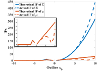
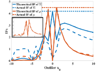
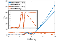
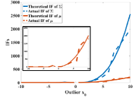
Proofs of the two lemmas are provided in the Appendices--C and -D. The actual and theoretical IF curves of the four EMMs are plotted in Fig. 1, showing that in practice the robustness of the EMMs can be well captured by our theoretical bounds.

More importantly, the robustness of the EMM can also be analysed from Lemmas 3 and 4, and is determined by $\psi_{k}(\cdot)$ (or $g_{k}(\cdot)$) of each cluster. Specifically, when $\mathbf{x}_{0}\rightarrow\infty$, $\mathcal{I}_{\mathbf{{\Sigma}}_{j}}(\mathbf{x}_{0})$ is bounded (defined as covariance robust) only when $\psi_{j}(t)t$ is bounded for $t\!\rightarrow\!\infty$, which leads to bounded $\psi_{j}(\overline{\mathbf{x}}_{0}^{T}\mathbf{\Sigma}_{j}^{-1}\overline{\mathbf{x}}_{0})\overline{\mathbf{x}}_{0}^{T}\mathbf{\Sigma}_{j}^{-1}\overline{\mathbf{x}}_{0}$ in (16). Likewise, bounded $\mathcal{I}_{\bm{\mu}_{j}}(\mathbf{x}_{0})$ (defined as mean robust) requires bounded $\psi_{j}(t)\sqrt{t}$, which is slightly more relaxed than the requirement of covariance robust. For example, in Fig. 1, by inspecting the boundedness of the curves, we find that the Gaussian and GG1.5 mixtures are neither covariance robust and mean robust, while the Cauchy mixtures are both covariance robust and mean robust. For the Laplace mixtures, they are not covariance robust but are mean robust, which shows that the covariance robust is more stringent than the mean robust. Thus, the developed bounds provide an extremely feasible and convenient treatment for qualifying or designing the robustness within EMMs.

V Experimental results

Our experimental settings are first detailed in Section V-A. We then employ in Section V-B two toy examples to illustrate the flexibility of EMMs in capturing different types of data. This also highlights the virtues of our method in universally solving EMMs. In Section V-C, we systematically compare our EMM solver with other baselines on the synthetic dataset, followed by a further evaluation on the image data of BSDS500 in Section V-D.

V-A Parameter settings and environments

Baselines: We compared the proposed method (Our) with the regular manifold optimisation (RMO) method without reformulation (i.e., updating $\bm{\mu}_{k}$ and $\mathbf{\Sigma}_{k}$ separately) and the IRA method, by optimising different EMMs over various data structures. It should be pointed out that the IRA includes a range of existing works on solving certain EMMs, e.g., the standard EM algorithm for the Gaussian distribution, [7] for the $t$-distribution and [11] for the hyperbolic distribution. Besides, the convergence criterion in all the experiments was set by the cost decrease of adjacent iterations of less than $10^{-10}$. For our method and the RMO, that involved manifold optimisation, we have utilised the default conjugate gradient solver in the Manopt toolbox [73]. We should also point out that we evaluated all the methods on original EMM problems and due to the fact that priors are highly data-dependent, we leave the reasonable and comprehensive evaluations on regularised EMMs as part of our future work.

Performance objectives: We compared our method with the RMO and IRA methods by comprehensively employing 9 different elliptical distributions as components within EMMs. These are listed in Table I, with their properties provided in Table II, where the Cauchy distribution is a special case of the student-$t$ distribution with $v=1$. We should also point out that the non-geodesic elliptical distributions cannot be solved by the IRA method [14, 15]. In contrast, as shown below, our method can provide a stable and fast solution even for the non-geodesic elliptical distributions.

TABLE I: Details of the 9 elliptical distributions used for assessments

	Gaussian	Student-$t$ ($v=1$ and $v=10$)	GG1.5	Logistic
$g(t)$ of (2)	$g(t)\propto\exp(-0.5t)$	$g(t)\propto(1+\nicefrac{{t}}{{v}})^{-\nicefrac{{(M+v)}}{{2}}}$	$g(t)\propto\exp(-0.5t^{1.5})$	$g(t)\propto\frac{\exp(-t)}{(1+\exp(-t))^{2}}$
	Laplace	Weib0.9	Weib1.1	Gamma1.1
$g(t)$ of (2)	$g(t)\propto\frac{\mathcal{K}_{(1-0.5M)}(\sqrt{2t})}{\sqrt{0.5t}^{0.5M-1}}$	$g(t)\propto t^{-0.1}\exp(-0.5t^{0.9})$	$g(t)\propto=t^{0.1}\exp(-0.5t^{1.1})$	$g(t)\propto t^{0.1}\exp(-0.5t)$
Note:	$\mathcal{K}_{x}(y)$ is the modified Bessel function of the second kind. Student-$t$ with $v=1$ is the Cauchy distribution.

TABLE II: Properties of the elliptical distributions used for evaluations

	Gaussian	Student-$t$	Laplace	GG1.5
Covariance Robust	No	Yes	No	No
Mean Robust	No	Yes	Yes	No
Heavily Tailed	No	Yes	Yes	No
Geodesic Convex	Yes	Yes	Yes	Yes
	Logistic	Weib0.9	Weib1.1	Gamma1.1
Covariance Robust	No	No	No	No
Mean Robust	No	No	No	No
Heavily Tailed	No	Yes	No	No
Geodesic Convex	Yes	Yes	No	No

Synthetic datasets: We generated the synthetic dataset via randomly choosing the mean and the covariance, except for the separation $c$ and eccentricity $e$ [36, 74], which were controlled to comprehensively evaluate the proposed method under various types of data structures. The separation, $c$, of two clusters $k_{1}$ and $k_{2}$ is defined as $||\bm{\mu}_{k_{1}}-\bm{\mu}_{k_{2}}||^{2}\geqslant c\cdot\max\{\mathrm{tr}(\mathbf{{{\Sigma}}}_{k_{1}}),\mathrm{tr}(\mathbf{{{\Sigma}}}_{k_{2}})\}$, and the eccentricity, $e$, is defined as a ratio of the largest and the smallest eigenvalue of the covariance matrix within one cluster. The smaller value of $c$ indicates the larger overlaps between clusters; the smaller value of $e$ means more spherically distributed clusters. In total, we generated $3\times 2=6$ types of synthetic datasets, whereby $M$ and $K$ were set in pairs to $\{8,8\}$, $\{16,16\}$, and $\{64,64\}$; $c$ and $e$ were set in pairs to $\{10,10\}$ and $\{0.1,1\}$ to represent the two extreme cases. Each synthetic dataset contained $10,000$ samples in total ($N=10,000$) drawn from different mixtures of Gaussian distributions. For each test case (i.e., for each method and for each EMM), we repeatedly ran the optimisation over $50$ trials, with random initialisations. Finally, we recorded average values of the iterations, the computational time and the final cost. When the optimisation failed, i.e., converging to singular covariance matrices or infinite negative likelihood, we also recorded and calculated the optimisation fail ratio within the $50$ initialisations for each test case, to evaluate the stability in optimisation.

BSDS500 dataset: Finally, we evaluated our method on the image data, over two typical tasks. The first was related to image segmentation, where all the 500 pictures in the Berkeley segmentation dataset BSDS500 [75] were tested and reported in our results. We set $K=2$ in this task in order to clearly show the effects of different EMMs in segmentation (as shown in Fig. 6). Evaluation over multiple parameters $K$ was included in the second task. Moreover, each optimisation was initialised by the k-means++ using the vl-feat toolbox [76], which is a typical initialisation method in clustering tasks such as the k-means clustering. The cost, iterations and computational time were recorded for all the 500 pictures. In the second task, our evaluation was implemented on another challenging task, by modelling and clustering $3\times 3$ and $5\times 5$ image patches from the image dataset. It needs to be pointed out that this task is a core part of many applications, such as image denoising, image super-resolution and image/video compression, where similarities of image patches play an important role. Specifically, we randomly extracted $100$ patches ($3\times 3$ and $5\times 5$) from each image in the BSDS500, and vectorised those patches as data samples. Thus, we finally obtained the test data with sizes $50,000\times 27$ and $50,000\times 75$, where $K$ was set to $3$ and $9$. Also, we ran each optimisation with $50$ times random initialisations, and recorded the average final cost and the standard deviation.

V-B Toy examples

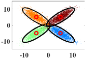
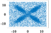
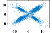
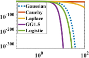
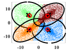
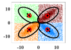
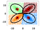
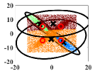
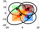
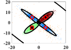
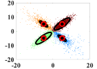
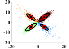
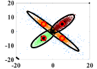
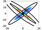
Before comprehensively evaluating our method, we first provide some intuition behind its performance based on flower-shaped data with 4 clusters ($N=10,000$) (shown in Fig. 2-(a)). The flexibility of the EMMs via our method is illustrated by: (i) adding 100$\%$ uniform noise (i.e., $10,000$ noisy samples), as shown in Fig. 2-(b); (ii) replacing two clusters by the Cauchy samples with the same mean and covariance matrices, as shown in Fig. 2-(c). The five distributions that were chosen as components in EMMs are shown in Fig. 2-(d).

The optimised EMMs are shown in Fig. 3. From this figure, we find that the GMM is inferior in modelling noisy or unbalanced data. This is mainly due to its lack of robustness, and thus similar results can be found in another non-robust EMM, i.e., the GG1.5. In contrast, for a robust EMM, such as the Cauchy and the Laplace, the desirable level of estimation is ensured in both cases. Therefore, a universal solver is crucial as it enables flexible EMMs can be well optimised for different types of data.

(a) Ground truth

(b) Case 1: $100\%$ Noise

(c) Case 2: Cauchy clusters

(d) Tails of distributions

Figure 2: Toy examples consisting of four Gaussian sets. (a) Data structure: The red circles represent the mean values at $(5,5)$, $(5,-5)$, $(-5,5)$ and $(-5,-5)$, and the black circles denote covariance ellipses including 95$\%$ data samples of each Gaussian distribution. (b) Test case adding 100$\%$ uniform noisy samples to the data. (c) Test case of data that consist of two Gaussian and two Cauchy sets. (d) Tails of the distributions which were utilised in this test. It needs to be pointed out that the Cauchy samples in (c) are spread over a wide range, so that we show (c) within $(\pm 15,\pm 15)$ for illustration convenience.

(a) Gaussian

(b) Cauchy

(c) Laplace

(d) Logistic

(e) GG1.5

Figure 3: Optimisation results of the proposed method across the 5 EMMs. The top row shows the results for Case 1 and the bottom row shows the results for Case 2. The red circles denote the ground-truth as shown in Fig. 2-(a), whilst the black crosses and ellipses represent the estimated mean and covariance matrices. The colour of each sample is corresponding to that of Fig. 2-(a), and is classified by selecting the maximum posterior among the clusters.

(a) Gaussian

(b) Cauchy

(c) Laplace

(d) Logistic

(e) GG1.5

Figure 4: Cost difference against the number of iterations of the 5 EMMs for Case 1. The top figures show the cost difference against the iterations optimised via Our, IRA and RMO methods. The bottom quantities are the final convergence speed in terms of the number of iterations and execution time (ites/sec).

(a) Gaussian

(b) Cauchy

(c) Laplace

(d) Logistic

(e) GG1.5

Figure 5: Cost difference against the number of iterations of the 5 EMMs for Case 2. The top figures show the cost difference against the iterations optimised via Our, IRA and RMO methods. The bottom quantities are the final convergence speed in terms of the number of iterations and execution time (ites/sec).

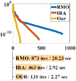
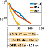
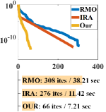
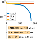
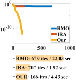
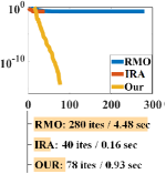
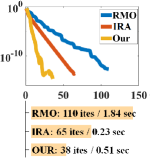
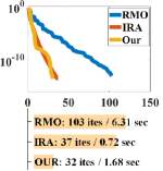
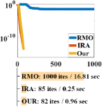
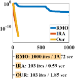
We further plot the iteration numbers against the average cost difference of Our, IRA and RMO methods when optimising the two cases in Fig. 4 and 5. Note that for the purpose of illustrations [16], the cost difference is defined by the absolute difference between the cost of each iteration and the relatively “optimal” cost, which was obtained by choosing the lowest value among the final costs of the three methods. From the two figures, the IRA achieved a monotonic convergence, because it consistently increases the lower bound of the log-likelihood; our method, although occasionally fluctuating at the late stage of convergence, such as for the Cauchy distribution in Fig. 5, consistently achieved the lowest cost among all EMMs and converged with the least number of iterations. A further cautious choice of optimisers as well as line search methods can probably achieve a monotonic convergence. Moreover, although one iteration of our method takes longer time than that of the IRA method due to the line search, the overall computational time of our method is comparable to that of the IRA method. As shown in the next section, our method even performs much faster in terms of computational time than the IRA for higher dimensions and larger numbers of clusters ($M>2$ and $K>4$).

TABLE III: Overall results averaged across $M$ and $K$ for 9 types of EMMs optimised by Our, IRA and RMO methods.

$c=10$, $e=10$		Gaussian	Cauchy	Student-$t$ ($v=10$)	GG1.5	Logistic	Weib0.9	Weib1.1	Gamma1.1	Mix
Our	Ite. / T. (s)	108 / 40.3	135 / 34.5	136 / 32.7	219 / 160	113 / 43.2	158 / 37.8	139 / 56.5	138 / 38.3	132 / 51.8
	Cost	64.5	65.6	64.8	69.8	47.8	64.4	64.4	64.4	67.5
IRA	Ite. / T. (s)	367 / 90.0	—-	—-	—-	428 / 249	310 / 46.8	—-	—-	—-
	Cost	66.2	—-	—-	—-	49.0	64.5	—-	—-	—-
RMO	Ite. / T. (s)	658 / 1738	848 / 1590	776 / 1681	796 / 1435	744 / 1651	825 / 1806	773 / 1625	760 / 1550	711 / 1547
	Cost	64.3	65.8	64.7	71.6	47.5	64.4	64.5	64.5	66.8
$c=0.1$, $e=1$
Our	Ite. / T. (s)	693 / 201	424 / 99.9	621 / 106	581 / 100	734 / 242	686 / 119	655 / 111	664 / 94.6	470 / 65.7
	Cost	40.0	41.0	40.2	39.8	23.5	39.1	40.1	40.1	39.2
IRA	Ite. / T. (s)	—-	—-	—-	—-	—-	711 / 101	—-	—-	—-
	Cost	—-	—-	—-	—-	—-	40.6	—-	—-	—-
RMO	Ite. / T. (s)	1000 / 1707	956 / 1661	951 / 1789	898 / 1206	963 / 1508	969 / 1632	975 / 1744	958 / 1561	917 / 1505
	Cost	40.4	41.5	40.8	42.1	23.8	40.3	40.5	40.4	40.4
Note:		T. (s): Time (seconds); Ite.: Iteration numbers; —-: Singularity or infinity in either $M=8$, $M=16$ or $M=64$.

TABLE IV: Detailed comparisons among Our, IRA and RMO on optimising 3 EMMs in the case of $c=10$ and $e=10$

(M, K)		Gaussian			Cauchy			Logistic
		Our	IRA	RMO	Our	IRA	RMO	Our	IRA	RMO
(8, 8)	T. (s)	3.70 $\pm$ 5.44	5.48 $\pm$ 4.13	4.23 $\pm$ 10.76	2.23 $\pm$ 1.67	3.04 $\pm$ 2.45	20.4 $\pm$ 10.6	4.28 $\pm$ 4.60	4.71 $\pm$ 4.08	18.9 $\pm$ 17.3
	Ite.	165 $\pm$ 240	538 $\pm$ 403	122 $\pm$ 308	107 $\pm$ 81.3	340 $\pm$ 275	640 $\pm$ 334	177 $\pm$ 191	463 $\pm$ 398	537 $\pm$ 489
	Co./Fa.	19.4 / 0$\%$	19.6 / 0$\%$	19.3 / 0$\%$	20.3 / 0$\%$	20.4 / 0$\%$	20.3 / 0$\%$	14.9 / 0$\%$	15.0 / 0$\%$	14.9 / 0$\%$
(16, 16)	T. (s)	15.8 $\pm$ 13.4	28.8 $\pm$ 15.2	221 $\pm$ 78.3	38.1 $\pm$ 34.5	40.9 $\pm$ 18.2	260 $\pm$ 1.84	15.7 $\pm$ 7.64	23.6 $\pm$ 14.6	193 $\pm$ 115
	Ite.	115 $\pm$ 94.0	400 $\pm$ 207	853 $\pm$ 304	272 $\pm$ 243	570 $\pm$ 254	1000 $\pm$ 0.00	115 $\pm$ 54.0	325 $\pm$ 201	734 $\pm$ 433
	Co./Fa.	37.7 / 0$\%$	38.0 / 0$\%$	37.8 / 0$\%$	38.7 / 0$\%$	38.8 / 0$\%$	39.0 / 0$\%$	28.6 / 0$\%$	28.8 / 0$\%$	28.6 / 0$\%$
(64, 64)	T. (s)	101 $\pm$ 18.0	236 $\pm$ 0.00	4988 $\pm$ 152	63.2 $\pm$ 11.7	—-	4491 $\pm$ 1549	110 $\pm$ 19.3	720 $\pm$ 343	4741 $\pm$ 475
	Ite.	45.8 $\pm$ 5.67	163 $\pm$ 0.00	1000 $\pm$ 0.00	26.9 $\pm$ 3.70	—-	902 $\pm$ 309	49.3 $\pm$ 5.98	497 $\pm$ 235	960 $\pm$ 121
	Co./Fa.	136 / 0$\%$	141 / 90$\%$	136 / 10$\%$	138 / 0$\%$	– / 100$\%$	138 / 0$\%$	99.7 / 0$\%$	103 / 70$\%$	99.1 / 10$\%$
Note:		T. (s): Time (seconds); Ite.: Iteration numbers; Co.: Final cost; Fa.: Optimisation fail ratio; —-: Singularity or infinity

V-C Evaluations over the synthetic datasets

We next systematically evaluated our method based on the synthetic dataset described in Section V-A. For each dataset, we had $8\times 3=24$ test cases, i.e., 9 types of EMMs for the 3 methods. The 9 types of EMMs include 7 types of elliptical distributions and the other one (denoted as Mix) is composed by half the number of Cauchy distributions and the other half of Gaussian distributions. Table III shows the overall result averaged across dimensions $M$ and $K$ for the 9 EMMs. As can be seen from Table III, our method exhibits the fastest convergence speed in terms of both the number of iterations and computation time, and it also obtains the minimum cost. It can also be found that datasets with more overlaps (i.e., $\{c=0.1,e=1\}$) take a longer time to optimise, whereby iterations and computational time increase for all the 3 methods. On the other hand, by comparing the results of our method and those of the RMO method, we can clearly see a significant improvement in both convergence speed and final minimum, which verifies the effectiveness of our reformulation technique.

We provide further details of the comparisons of different $M$ and $K$ in Table IV, where 3 EMMs and $\{c=10,e=10\}$ were reported due to the space limitation and the fact that similar results can be found for other EMMs and settings of Table III. We can see from this table that the superior performance of our method is consistent over different dimensions $M$ and cluster numbers $K$. Table IV shows that our method requires the minimum number of iterations as well as least computational time. More importantly, the standard deviations for the iterations and computational time of our method are almost the lowest, which means that our method is able to stably optimise the EMMs. With an increase in $M$ and $K$, our method consistently achieves the best performance of the average costs with $0\%$ fail ratio. In contrast, the IRA can become extremely unstable. One reason is due to the fact that, as mentioned in Section II-C, the IRA cannot converge for the non-geodesic convex distributions such as the Weib1.1 and Gamma1.1 in Table III [40]. Another perspective is that it even failed on geodesic convex distributions in Table IV (e.g., $90\%$ fail ratio for the Gaussian and $100\%$ fail ratio for the Cauchy when $M\!=\!64,K\!=\!64$). This may be due to the separate updating scheme on $\bm{\mu}_{k}$ and $\mathbf{\Sigma}_{k}$, which has been mentioned in Section III-B. Although we see an enhanced stability when using manifold optimisation, this separate updating scheme, we believe, is also the reason that the RMO requires extremely large computational complexity to converge ($>900$ iterations and $>4000$ seconds when $M\!=\!64,K\!=\!64$) and in several cases it even failed to converge altogether. Our method, on the one hand, re-parametrises the parameters to perform a simultaneous update on $\bm{\mu}_{k}$ and $\mathbf{\Sigma}_{k}$ via $\mathbf{\tilde{\Sigma}}_{k}$; the re-parametrised EMMs also have a fixed zero mean that prevents potential clusters to move to the data boundary. These two aspects enable our method to consistently and stably optimise EMMs with the fastest convergence speed and lowest cost.

(a) Original

(b) Gaussian

(c) Cauchy

(d) Laplace

(e) Logistic

(f) GG1.5

Figure 6: Reconstructed images by Our method when optimising the 5 EMMs.

TABLE V: Comparisons averaged over 500 pictures among Our, the IRA and the RMO for estimating the 5 EMMs

	Gaussian			Cauchy			Laplace			GG1.5			Logistic
	Our	IRA	RMO	Our	IRA	RMO	Our	IRA	RMO	Our	IRA	RMO	Our	IRA	RMO
Iterations	56	234	954	87	390	939	101	288	962	61	224	982	58	239	965
Time (s)	5.55	11.8	165	7.12	16.8	159	20.4	42.2	486	8.32	14.4	205	6.73	13.3	177
Cost	12.3	12.3	12.3	12.1	12.4	12.3	12.2	12.2	12.3	12.4	12.4	12.4	11.1	11.1	11.2
SSIM [77]	0.5930			0.6052			0.6112			0.5813			0.5792

TABLE VI: Comparisons among Our (with different manifold solvers), IRA and RMO methods on the BSDS500 image patches

	Gaussian					Cauchy
$K,M=3,27$	Our	Our (STP)	Our (LBF)	IRA	RMO	Our	Our (STP)	Our (LBF)	IRA	RMO
Time (s)	28.3$\pm$7.62	210$\pm$109	102$\pm$8.67	155$\pm$37.0	486$\pm$197	118$\pm$72.9	224$\pm$106	302$\pm$139	—-	556$\pm$26.2
Iterations	109$\pm$27.5	749$\pm$390	318$\pm$37.3	930$\pm$221	844$\pm$342	416$\pm$254	817$\pm$387	670$\pm$253	—-	983$\pm$54.4
Cost	72.8$\pm$1.30	73.6$\pm$6.30	72.0$\pm$1.84	73.9$\pm$2.01	75.5$\pm$6.72	70.7$\pm$1.53	69.5$\pm$4.63	70.5$\pm$1.47	—-	70.7$\pm$1.82
$K,M=9,75$	Our	Our (STP)	Our (LBF)	IRA	RMO	Our	Our (STP)	Our (LBF)	IRA	RMO
Time (s)	170$\pm$23.3	125$\pm$34.1	1609$\pm$74.7	—-	4568$\pm$904	595$\pm$473	2025$\pm$38.6	898$\pm$157	—-	4389$\pm$1229
Iterations	90.0$\pm$8.80	63.0$\pm$25.5	998$\pm$7.07	—-	921$\pm$177	295$\pm$230	1e3$\pm$0	394$\pm$93.0	—-	918$\pm$259
Cost	160$\pm$3.33	178$\pm$21.1	160$\pm$2.89	—-	172$\pm$0.31	170$\pm$0.25	171$\pm$3.32	171$\pm$2.37	—-	173$\pm$4.31

V-D BSDS500 dataset:

Convergence speed between Our, the IRA, and the RMO methods was compared over averaged results across the whole 500 pictures in BSDS500, as shown in Table V. Again, our method converged with the fastest speed and achieved the minimum cost error among the RMO and the IRA methods. We further show in Fig. 6 four reconstructed images via our method when optimising the five EMMs. Observe that the images reconstructed from the non-robust distributions (e.g., the Gaussian and the GG1.5 distributions) were more “noisy” than those from the robust distributions (e.g., the Cauchy and Laplace distributions); however, these may capture more details in images. Thus, by our method, different EMMs can flexibly model data for different requirements or applications.

Finally, we evaluated our method on modelling the BSDS500 image patches, which is a challenging but important task in practice. More comprehensively, besides the manifold conjugate gradient solver adopted as a default of our method, we further evaluated the manifold steepest descent (denoted as Our (STP)) and the manifold LBFGS (denoted as Our (LBF)) as alternatives to solve the step descent in Algorithm 1. The results are reported in Table VI. From this table, we can see again that our method consistently achieved the lowest costs across different initialisations. For example, for the Gaussian mixtures, it obtained $72.8\pm 1.30$ in the $50$ random initialisations, compared to $73.9\pm 2.01$ of the IRA and $75.5\pm 6.72$ of the RMO. Also, our method converged with the least computational time and was able, compared to the existing methods, to consistently provide fast, stable and superior optimisation. Furthermore, by employing different solvers, the results achieved by our method are comparable to one another; among the three solvers, the steepest descent solver took slightly more computational time due to its naive update rule, whilst the conjugate gradient solver performed slightly better than the other two solvers in balancing the computational time and cost. Overall, all the three solvers of our method achieved much better results than the IRA and the RMO methods, which also verifies the effectiveness of our re-designed cost. Therefore, we can conclude that for various scenarios and applications, our method was able to consistently yield a superior model with the lowest computational time.

VI Conclusions

We have proposed a general framework for a systematic analysis and universal optimisation of the EMMs, and have conclusively demonstrated that this equips EMMs with significantly enhanced flexibility and ease of use in practice. In addition to the general nature and the power of the proposed universal framework for EMMs, we have also verified both analytically and through simulations, that this provides a reliable and robust statistical tool for analysing the EMMs. Furthermore, we have proposed a general solver which consistently attains the optimum for general EMMs. Comprehensive simulations over both synthetic and real-world datasets validate the proposed framework, which is fast, stable and flexible.

-A Proof of Lemma 1

To calculate the Riemannian metric for the covariance matrix, we follow the work of [53] to calculate the Hessian of the Boltzman entropy of elliptical distributions. The Boltzman entropy is first obtained as follows,

$$H(\mathbf{x}|\mathbf{{\Sigma}}) =\int_{\mathbf{x}}p_{\mathbf{x}}(\mathbf{x})\ln p_{\mathbf{x}}(\mathbf{x})d\mathbf{x}$$ (20)

$$=\int_{\mathbf{x}}p_{\mathbf{x}}(\mathbf{x})[-\frac{1}{2}\ln|\mathbf{{\Sigma}}|+\ln c_{M}+\ln g(t)]d\mathbf{x}$$

$$=-\frac{1}{2}\ln|\mathbf{\Sigma}|+\ln c_{M}+\int_{\mathbb{R}^{M}}p_{\mathcal{R}}(t)\ln g(t)dt.$$

Because $(\ln c_{M}+\int_{\mathbb{R}^{M}}p_{\mathcal{R}}(t)\ln g(t)dt)$ is irrelevant to $\mathbf{{\Sigma}}$, the Hessian of $H(\mathbf{x}|\mathbf{{\Sigma}})$ can be calculated as

$$\frac{\partial H(\mathbf{x}|\mathbf{{\Sigma}}+s{\mathbf{\Sigma}_{0}}+h\mathbf{\Sigma}_{1})}{\partial s\partial h}|_{s=0,h=0}=\frac{1}{2}\mathrm{tr}({\mathbf{\Sigma}_{0}}\mathbf{\Sigma}^{-1}{\mathbf{\Sigma}_{1}}\mathbf{\Sigma}^{-1}).$$ (21)

The Riemannian metric can thus be obtained as $ds^{2}=\frac{1}{2}\mathrm{tr}(d\mathbf{\Sigma}\mathbf{{\Sigma}}^{-1}d\mathbf{\Sigma}\mathbf{{\Sigma}}^{-1})$, which is the same as the case for multivariate normal distributions and is the mostly widely used metric.

This completes the proof of Lemma 1.

-B Proof of Theorem 1

The proof of this property rests upon an expansion $\mathbf{y}_{n}^{T}\mathbf{\tilde{\Sigma}}_{k}^{-1}\mathbf{y}_{n}$ to become $(\mathbf{x}_{n}-\bm{\mu}_{k})^{T}\mathbf{\Sigma}_{k}^{-1}(\mathbf{x}_{n}-\bm{\mu}_{k})+\frac{1}{\lambda_{k}}$ within derivatives of $\tilde{J}$. By setting $\nicefrac{{\partial\tilde{J}}}{{\partial\lambda_{k}}}=0$ and $\nicefrac{{\partial\tilde{J}}}{{\partial c_{k}}}=0$, we then arrive at

$$\lambda_{k} =-2\frac{\sum_{n=1}^{N}\tilde{\xi}_{nk}\psi_{k}(t_{nk}+\frac{1}{\lambda_{k}}-c_{k})}{\sum_{n=1}^{N}\tilde{\xi}_{nk}},$$ (22)

$$c_{k} =-\frac{1}{2}\frac{\sum_{n=1}^{N}\tilde{\xi}_{nk}}{\sum_{n=1}^{N}\tilde{\xi}_{nk}\psi_{k}(t_{nk}+\frac{1}{\lambda_{k}}-c_{k})},$$

where

$$\tilde{\xi}_{nk}\!=\!\frac{\pi_{k}\cdot c_{M}\cdot\sqrt{c_{k}\cdot\mathrm{det}(\mathbf{\tilde{\Sigma}}_{k}^{-1})}\cdot g_{k}\left(\mathbf{y}_{n}^{T}\mathbf{\tilde{\Sigma}}_{k}^{-1}\mathbf{y}_{n}-c_{k}\right)}{\sum_{k=1}^{K}\pi_{k}\cdot c_{M}\cdot\sqrt{c_{k}\cdot\mathrm{det}(\mathbf{\tilde{\Sigma}}_{k}^{-1})}\cdot g_{k}\left(\mathbf{y}_{n}^{T}\mathbf{\tilde{\Sigma}}_{k}^{-1}\mathbf{y}_{n}\!-\!c_{k}\right)}.$$ (23)

By inspecting $\lambda_{k}=\nicefrac{{1}}{{c_{k}}}$, $\mathrm{det}(\mathbf{\tilde{\Sigma}}_{k})=\lambda_{k}\cdot\mathrm{det}(\mathbf{\Sigma}_{k})$ and $\mathbf{y}_{n}^{T}\mathbf{\tilde{\Sigma}}_{k}^{-1}\mathbf{y}_{n}=(\mathbf{x}_{n}-\bm{\mu}_{k})^{T}\mathbf{\Sigma}_{k}^{-1}(\mathbf{x}_{n}-\bm{\mu}_{k})+\frac{1}{\lambda_{k}}$, we obtain $\tilde{\xi}_{nk}=\xi_{nk}$ and $\psi_{k}(t_{nk}+\frac{1}{\lambda_{k}}-c_{k})=\psi_{k}(t_{nk})$.

To prove the equivalence of the optimum of $\mathbf{\tilde{\Sigma}}_{k}$ in (10) and optima of $\bm{\mu}_{k}$ and $\mathbf{\Sigma}_{k}$, we directly calculate $\nicefrac{{\partial\tilde{J}}}{{\partial\mathbf{\tilde{\Sigma}}_{k}}}$ in (10) and set it to $0$, to yield

$$\mathbf{\tilde{\Sigma}}_{k}=-2\frac{\sum_{n=1}^{N}\tilde{\xi}_{nk}\psi_{k}(t_{nk}+\frac{1}{\lambda_{k}}-c_{k})\mathbf{y}_{n}\mathbf{y}_{n}^{T}}{\sum_{n=1}^{N}\tilde{\xi}_{nk}}.$$ (24)

Again, as $\lambda_{k}=\nicefrac{{1}}{{c_{k}}}$ and $\tilde{\xi}_{nk}=\xi_{nk}$, we arrive at

$$\mathbf{\tilde{\Sigma}}_{k} =-2\frac{\sum_{n=1}^{N}\xi_{nk}\psi_{k}(t_{nk})\mathbf{y}_{n}\mathbf{y}_{n}^{T}}{\sum_{n=1}^{N}\xi_{nk}}$$ (25)

$$=-2\frac{\sum_{n=1}^{N}\xi_{nk}\psi_{k}(t_{nk})}{\sum_{n=1}^{N}\xi_{nk}}\begin{bmatrix}\mathbf{x}_{n}\mathbf{x}_{n}^{T}&\mathbf{x}_{n}\\ \mathbf{x}_{n}^{T}&1\\ \end{bmatrix}.$$

By substituting $\bm{\mu}_{k}$ and $\mathbf{\Sigma}_{k}$ of (7) and $\lambda_{k}$ in (22), we have

$$\mathbf{\tilde{\Sigma}}_{k}=\begin{bmatrix}\mathbf{\Sigma}_{k}+\lambda_{k}\bm{\mu}_{k}\bm{\mu}_{k}^{T}&\lambda_{k}\bm{\mu}_{k}\\ \lambda_{k}\bm{\mu}_{k}^{T}&\lambda_{k}\\ \end{bmatrix},$$ (26)

which means that the optimum value $\mathbf{\tilde{\Sigma}}_{k}$ is exactly the reformulated form by the optimum values of (7).

This completes the proof of Theorem 1.

-C Proof of Lemma 3

We here denote the contaminated distribution $\mathcal{F}=(1-\epsilon)\mathcal{F}_{\mathbf{x}}+\epsilon\mathcal{F}_{\mathbf{x}_{0}}$, where $\epsilon$ is the proportion of outliers; $\mathcal{F}_{\mathbf{x}}$ is the true distribution of $\mathbf{x}$ and $\mathcal{F}_{\mathbf{x}_{0}}$ is the point-mass distribution at $\mathbf{x}_{0}$. For simplicity, we employ $t$ to denote $(\mathbf{x}-\bm{\mu}_{j})^{T}\mathbf{\Sigma}_{j}^{-1}(\mathbf{x}-\bm{\mu}_{j})$ and $t_{0}$ to denote $(\mathbf{x}_{0}-\bm{\mu}_{j})^{T}\mathbf{\Sigma}_{j}^{-1}(\mathbf{x}_{0}-\bm{\mu}_{j})$. Then, the maximum log-likelihood estimation on the $\mathbf{\Sigma}_{j}$ of $\mathcal{E}_{j}(\bm{\mu}_{j},\mathbf{\Sigma}_{j},g_{j})$ becomes

$$(1-\epsilon)\mathbb{E}[\xi_{j}(\mathbf{x})\psi_{j}(t)(\mathbf{x}-\bm{\mu}_{j})(\mathbf{x}-\bm{\mu}_{j})^{T}+\frac{1}{2}\xi_{j}(\mathbf{x})\mathbf{\Sigma}_{j}]$$ (27)

$$+\epsilon\xi_{j}(\mathbf{x}_{0})\psi_{j}(t_{0})(\mathbf{x}_{0}-\bm{\mu}_{j})(\mathbf{x}_{0}-\bm{\mu}_{j})^{T}+\epsilon\frac{\xi_{j}(\mathbf{x}_{0})}{2}\mathbf{\Sigma}_{j}=0.$$

We first calculate the IF (denoted by $\mathcal{I}$ in the proof) when $\mathbf{\Sigma}_{j}=\mathbf{I}$ and $\bm{\mu}_{j}=\mathbf{0}$. Thus, we have $t=\mathbf{x}^{T}\mathbf{x}$ and $t_{0}=\mathbf{x}_{0}^{T}\mathbf{x}_{0}$ in the following proof. Then, according to the definition of IF, we differentiate (27) with respect to $\epsilon$ and when it approaches $0$, we arrive at

$$\mathbb{E}\big{[}\frac{\partial\xi_{j}(\mathbf{x})}{\partial\epsilon}|_{\epsilon=0}\psi_{j}(t)\mathbf{x}\mathbf{x}^{T}$$ (28)

$$\!+\!\xi_{j}(\mathbf{x})\frac{\partial\psi_{j}(\mathbf{x}^{T}\mathbf{\Sigma}_{j}^{-1}\mathbf{x})}{\partial\epsilon}|_{\epsilon=0}\mathbf{x}\mathbf{x}^{T}\!+\!\frac{1}{2}\frac{\partial\xi_{j}(\mathbf{x})}{\partial\epsilon}|_{\epsilon=0}\mathbf{I}\!+\!\frac{1}{2}\xi_{j}(\mathbf{x})\mathcal{I}\big{]}$$

$$+\xi_{j}(\mathbf{x}_{0})\psi_{j}(t_{0})\mathbf{x}_{0}\mathbf{x}_{0}^{T}+\frac{1}{2}\xi_{j}(\mathbf{x}_{0})\mathbf{I}=0.$$

In addition, we obtain

$$\frac{\partial\xi_{j}(\mathbf{x})}{\partial\epsilon}|_{\epsilon=0} =(\xi_{j}(\mathbf{x})-\xi_{j}^{2}(\mathbf{x}))\cdot(-\frac{1}{2}\mathrm{tr}(\mathcal{I})-\psi_{j}(t)\mathbf{x}^{T}\mathcal{I}\mathbf{x}),$$ (29)

$$\frac{\partial\xi_{j}(\mathbf{x})}{\partial\epsilon}|_{\epsilon=0} =-\psi^{\prime}_{j}(t)\mathbf{x}^{T}\mathcal{I}\mathbf{x}.$$

By combining (28) and (29), we arrive at

$$\mathbb{E}\big{[}(\xi_{j}(\mathbf{x})\!-\!\xi_{j}^{2}(\mathbf{x})) \!\cdot\!(-\frac{1}{2}\mathrm{tr}(\mathcal{I})\!-\!\psi_{j}(t)\mathbf{x}^{T}\mathcal{I}\mathbf{x})\!\cdot\!(\psi_{j}(t)\mathbf{x}\mathbf{x}^{T}\!+\!\frac{1}{2}\mathbf{I})$$ (30)

$$-\xi_{j}(\mathbf{x})\psi^{\prime}_{j}(t)(\mathbf{x}^{T}\mathcal{I}\mathbf{x})\mathbf{x}\mathbf{x}^{T}+\frac{1}{2}\xi_{j}(\mathbf{x})\mathcal{I}\big{]}$$

$$~{}~{}~{}~{}+\xi_{j}(\mathbf{x}_{0})\psi_{j}(t_{0})\mathbf{x}_{0}\mathbf{x}_{0}^{T}+\frac{1}{2}\xi_{j}(\mathbf{x}_{0})\mathbf{I}=0.$$

It should be pointed out that $(\mathbf{x}-\bm{\mu})^{T}\mathbf{\Sigma}^{-1}(\mathbf{x}-\bm{\mu})$ has the same distribution as $\mathcal{R}^{2}$. It is thus independent of $\frac{\Sigma^{-\nicefrac{{1}}{{2}}}(\mathbf{x}-\bm{\mu})}{\sqrt{(\mathbf{x}-\bm{\mu})^{T}\mathbf{\Sigma}(\mathbf{x}-\bm{\mu})}}$ (denoted by $\mathbf{u}$), which has the same distribution as $\mathcal{S}$ (i.e., uniform distribution). For mixing components, when data are well-separated, those $\mathbf{x}$ that do not belong to the $j$-th cluster have extremely low $\xi_{j}(\mathbf{x})$. In other words, the expectation in (30) is dominated by the expectation of the data which belong to the $j$-th cluster. Therefore, to calculate the expectation, we can treat the quadratic term $(\mathbf{x}-\mathbf{0})^{T}\mathbf{I}(\mathbf{x}-\mathbf{0})=\mathbf{x}^{T}\mathbf{x}$ (i.e., $t$) as independent of the normalised term $\frac{\mathbf{I}^{-\nicefrac{{1}}{{2}}}(\mathbf{x}-\mathbf{0})}{\sqrt{t}}=\frac{\mathbf{x}}{\sqrt{t}}$ (i.e., $\mathbf{u}$) of the $j$-th cluster.

Based on this approximation, we can rewrite (30) as

$$\mathbb{E}\big{[}(\xi_{j}(t)\!-\!\xi_{j}^{2}(t)) \!\cdot\!(\!-\!\frac{1}{2}\mathrm{tr}(\mathcal{I})\!-\!\psi_{j}(t)t\cdot\mathbf{u}^{T}\mathcal{I}\mathbf{u})\!\cdot\!(\psi_{j}(t)t\!\cdot\!\mathbf{u}\mathbf{u}^{T}\!+\!\frac{1}{2}\mathbf{I})$$ (31)

$$\!-\!\xi_{j}(t)\psi^{\prime}_{j}(t)t^{2}(\mathbf{u}^{T}\mathcal{I}\mathbf{u})\mathbf{u}\mathbf{u}^{T}\!+\!\frac{1}{2}\xi_{j}(t)\mathcal{I}\big{]}$$

$$~{}~{}~{}~{}+\xi_{j}(\mathbf{x}_{0})\psi_{j}(t_{0})\mathbf{x}_{0}\mathbf{x}_{0}^{T}+\frac{1}{2}\xi_{j}(\mathbf{x}_{0})\mathbf{I}=0.$$

Moreover, as $\mathbf{u}$ is uniformly distributed, we have $\mathbb{E}[\mathbf{u}\mathbf{u}^{T}]=\frac{1}{M}\mathbf{I}$, $\mathbb{E}[\mathbf{u}^{T}\mathcal{I}\mathbf{u}]=\frac{1}{M}\mathrm{tr}(\mathcal{I})$ and $\mathbb{E}[(\mathbf{u}^{T}\mathcal{I}\mathbf{u})\mathbf{u}\mathbf{u}^{T}]=\frac{1}{M(M+1)}(\mathcal{I}+\mathrm{tr}(\mathcal{I})\mathbf{I})$. Thus, we arrive at

$$\!-\!\frac{(\mathbb{E}\big{[}(\xi_{j}(t)\!-\!\xi_{j}^{2}(t))\psi_{j}^{2}(t)t^{2}\big{]}+\mathbb{E}\big{[}\xi_{j}(t)\psi^{\prime}_{j}(t)t^{2}\big{]})(\mathcal{I}+\mathrm{tr}(\mathcal{I})\mathbf{I})}{M(M+1)}$$ (32)

$$\!-\!\frac{\mathbb{E}\big{[}(\xi_{j}(t)\!-\!\xi_{j}^{2}(t))\psi_{j}(t)t\big{]}\mathrm{tr}(\mathcal{I})}{2M}\mathbf{I}\!-\!\frac{\mathbb{E}[(\xi_{j}(t)\!-\!\xi_{j}^{2}(t))]\mathrm{tr}(\mathcal{I})}{4}\mathbf{I}$$

$$-\frac{1}{2M}\mathbb{E}[(\xi_{j}(t)-\xi_{j}^{2}(t))\psi_{j}(t)t]\mathrm{tr}(\mathcal{I})\mathbf{I}+\frac{\pi_{j}}{2}\mathcal{I}$$

$$+\xi_{j}(\mathbf{x}_{0})\psi_{j}(t_{0})\mathbf{x}_{0}\mathbf{x}_{0}^{T}+\frac{1}{2}\xi_{j}(\mathbf{x}_{0})\mathbf{I}=0.$$

With $w_{1}$ and $w_{2}$ in (17), we can re-write (32) as

$$w_{2}\mathcal{I}=w_{1}\mathrm{tr}(\mathcal{I})\mathbf{I}-\xi_{j}(\mathbf{x}_{0})\psi_{j}(t_{0})\mathbf{x}_{0}\mathbf{x}_{0}^{T}-\frac{1}{2}\xi_{j}(\mathbf{x}_{0})\mathbf{I}.$$ (33)

Then, by taking the trace on both sides of (33), we have

$$\mathrm{tr}(\mathcal{I})=\frac{\xi_{j}(\mathbf{x}_{0})\psi_{j}(t_{0})\mathbf{x}_{0}\mathbf{x}_{0}^{T}+\frac{1}{2}\xi_{j}(\mathbf{x}_{0})\mathbf{I}}{Mw_{1}-w_{2}}$$ (34)

Thus, the IF at point $\mathbf{x}_{0}$ of the $j$-th cluster, when $\mathbf{\Sigma}_{j}=\mathbf{I}$, can be obtained as

$$\mathcal{I}(\mathbf{x}_{0})= \left[\frac{2w_{1}\cdot\xi_{j}(\mathbf{x}_{0})\psi_{j}(\mathbf{x}_{0}^{T}\mathbf{x}_{0})\mathbf{x}_{0}^{T}\mathbf{x}_{0}+w_{2}\cdot\xi_{j}(\mathbf{x}_{0})}{2(Mw_{1}-w_{2})w_{2}}\right]\cdot\mathbf{I}$$ (35)

$$-\frac{\xi_{j}(\mathbf{x}_{0})\psi_{j}(\mathbf{x}_{0}^{T}\mathbf{x}_{0})}{w_{2}}\mathbf{x}_{0}\mathbf{x}_{0}^{T}.$$

The IF is then obtained at point $\mathbf{x}_{0}$ of the $j$-th cluster for general $\mathbf{\Sigma}_{j}$ and $\bm{\mu}_{j}$ according to its affine equivalence (i.e., $\mathcal{I}_{\mathbf{\Sigma}_{j}}(\mathbf{x}_{0})=\mathbf{\Sigma}_{j}^{\nicefrac{{1}}{{2}}}\mathcal{I}(\mathbf{\Sigma}_{j}^{-\nicefrac{{1}}{{2}}}(\mathbf{x}_{0}-\bm{\mu}_{j}))\mathbf{\Sigma}_{j}^{\nicefrac{{1}}{{2}}}$).

This completes the proof of Lemma 3.

-D Proof of Lemma 4

Similar to the proof of Lemma 3, we have the following equation for estimating $\bm{\mu}_{j}$ with contaminated distribution $\mathcal{F}=(1-\epsilon)\mathcal{F}_{\mathbf{x}}+\epsilon\mathcal{F}_{\mathbf{x}_{0}}$:

$$(1-\epsilon)\mathbb{E}[\xi_{j}(\mathbf{x})\psi_{j}(t)\mathbf{\Sigma}_{j}^{-1} (\mathbf{x}-\bm{\mu}_{j})]$$ (36)

$$\!+\!\epsilon\xi_{j}(\mathbf{x}_{0})\psi_{j}(t_{0})\mathbf{\Sigma}_{j}^{-1}(\mathbf{x}_{0}-\bm{\mu}_{j})=0$$

Note that in (36), for simplicity we also use $t$ to denote $(\mathbf{x}-\bm{\mu}_{j})^{T}\mathbf{\Sigma}_{j}^{-1}(\mathbf{x}-\bm{\mu}_{j})$ and $t_{0}$ to denote $(\mathbf{x}_{0}-\bm{\mu}_{j})^{T}\mathbf{\Sigma}_{j}^{-1}(\mathbf{x}_{0}-\bm{\mu}_{j})$. We here also utilise $\mathcal{I}$ to denote the IF in this proof.

In addition, by differentiating with $\epsilon$ and $\epsilon\rightarrow 0$, we arrive at

$$\mathbb{E}\big{[}\frac{\partial\xi_{j}(\mathbf{x})}{\partial\epsilon}|_{\epsilon=0}\psi_{j}(t)\mathbf{\Sigma}_{j}^{-1}(\mathbf{x}-\bm{\mu}_{j})$$ (37)

$$~{}~{}~{}~{}+\xi_{j}(\mathbf{x})\frac{\partial\psi_{j}(t)}{\partial\epsilon}|_{\epsilon=0}\mathbf{\Sigma}_{j}^{-1}(\mathbf{x}-\bm{\mu}_{j})-\xi_{j}(\mathbf{x})\psi_{j}(t)\mathbf{\Sigma}_{j}^{-1}\mathcal{I}\big{]}$$

$$~{}~{}~{}~{}~{}~{}~{}~{}~{}~{}~{}~{}~{}~{}~{}~{}~{}~{}~{}~{}~{}~{}~{}~{}~{}~{}~{}+\xi_{j}(\mathbf{x}_{0})\psi_{j}(t_{0})\mathbf{\Sigma}_{j}^{-1}(\mathbf{x}_{0}-\bm{\mu}_{j})=0.$$

Besides, we also calculate

$$\frac{\partial\xi_{j}(\mathbf{x})}{\partial\epsilon}|_{\epsilon=0} =(\xi_{j}(\mathbf{x})-\xi_{j}^{2}(\mathbf{x}))\cdot(-2\psi_{j}(t)(\mathbf{x}-\bm{\mu}_{j})^{T}\mathbf{\Sigma}_{j}^{-1}\mathcal{I})$$ (38)

$$\frac{\partial\psi_{j}(\mathbf{x})}{\partial\epsilon}|_{\epsilon=0} =-2\psi^{\prime}_{j}(t)(\mathbf{x}-\bm{\mu}_{j})^{T}\mathbf{\Sigma}_{j}^{-1}\mathcal{I}.$$

When data are well separated, we can assume that $t=(\mathbf{x}-\bm{\mu}_{j})^{T}\mathbf{\Sigma}_{j}^{-1}(\mathbf{x}-\bm{\mu}_{j})$ is independent of $\mathbf{u}=\frac{\mathbf{\Sigma}_{j}^{-\nicefrac{{1}}{{2}}}(\mathbf{x}-\bm{\mu}_{j})}{\sqrt{t}}$. Therefore, (38) becomes

$$2\!\cdot\!\mathbb{E}\big{[}(\xi_{j}(\mathbf{x})-\xi_{j}^{2}(\mathbf{x}))\psi_{j}^{2}(t)t\big{]}\!\cdot\!\mathbb{E}\big{[}\mathbf{u}^{T}\mathbf{\Sigma}_{j}^{-\frac{1}{2}}\mathcal{I}\mathbf{u}\big{]}$$ (39)

$$\!+\!2\!\cdot\!\mathbb{E}\big{[}\xi_{j}(\mathbf{x})\psi^{\prime}_{j}(t)t\big{]}\!\cdot\!\mathbb{E}\big{[}\mathbf{u}^{T}\mathbf{\Sigma}_{j}^{-\frac{1}{2}}\mathcal{I}\mathbf{u}\big{]}\!+\!\mathbb{E}[\xi_{j}(\mathbf{x})\psi_{j}(t)]\mathbf{\Sigma}_{j}^{-\frac{1}{2}}\mathcal{I}$$

$$=\xi_{j}(\mathbf{x}_{0})\psi_{j}(t_{0})\mathbf{\Sigma}_{j}^{-\frac{1}{2}}(\mathbf{x}_{0}-\bm{\mu}_{j}),$$

which yields $\mathbb{E}[\mathbf{u}^{T}\mathbf{\Sigma}_{j}^{-\frac{1}{2}}\mathcal{I}\mathbf{u}]=\frac{1}{M}\mathbf{\Sigma}_{j}^{-\frac{1}{2}}\mathcal{I}$. Thus, we arrive at

$$\mathcal{I}\!=\!\frac{\xi_{j}(\mathbf{x}_{0})\psi_{j}(t_{0})(\mathbf{x}_{0}-\bm{\mu}_{j})}{\frac{2}{M}\mathbb{E}[(\xi_{j}(\mathbf{x})-\xi_{j}^{2}(\mathbf{x}))\psi_{j}^{2}(t)t]\!+\!\frac{2}{M}\mathbb{E}[\xi_{j}(\mathbf{x})\psi^{\prime}_{j}(t)t]\!+\!\mathbb{E}[\xi_{j}(\mathbf{x})\psi_{j}(t)]}.$$ (40)

This completes the proof of Lemma 4.

References

- [1] M. A. T. Figueiredo and A. K. Jain, “Unsupervised learning of finite mixture models,” IEEE Transactions on Pattern Analysis and Machine Intelligence, vol. 24, no. 3, pp. 381–396, 2002.
- [2] A. M. Zoubir, V. Koivunen, Y. Chakhchoukh, and M. Muma, “Robust estimation in signal processing: A tutorial-style treatment of fundamental concepts,” IEEE Signal Processing Magazine, vol. 29, no. 4, pp. 61–80, 2012.
- [3] D. P. Mandic, D. Obradovic, A. Kuh, T. Adali, U. Trutschell, M. Golz, P. De Wilde, J. Barria, A. Constantinides, and J. Chambers, “Data fusion for modern engineering applications: An overview,” in Proceeding of International Conference on Artificial Neural Networks. Springer, 2005, pp. 715–721.
- [4] K. W. Fang, S. Kotz, and K. W. Ng, Symmetric multivariate and related distributions. London, U.K.: Chapman & Hall, 1990.
- [5] P. J. Huber, “Robust statistics,” in International Encyclopedia of Statistical Science. Springer, 2011, pp. 1248–1251.
- [6] H. Holzmann, A. Munk, and T. Gneiting, “Identifiability of finite mixtures of elliptical distributions,” Scandinavian Journal of Statistics, vol. 33, no. 4, pp. 753–763, 2006.
- [7] D. Peel and G. J. McLachlan, “Robust mixture modelling using the t distribution,” Statistics and Computing, vol. 10, no. 4, pp. 339–348, 2000.
- [8] J. L. Andrews and P. D. McNicholas, “Model-based clustering, classification, and discriminant analysis via mixtures of multivariate t-distributions,” Statistics and Computing, vol. 22, no. 5, pp. 1021–1029, 2012.
- [9] T.-I. Lin, P. D. McNicholas, and H. J. Ho, “Capturing patterns via parsimonious t mixture models,” Statistics & Probability Letters, vol. 88, pp. 80–87, 2014.
- [10] S. Tan and L. Jiao, “Multivariate statistical models for image denoising in the wavelet domain,” International Journal of Computer Vision, vol. 75, no. 2, pp. 209–230, 2007.
- [11] R. P. Browne and P. D. McNicholas, “A mixture of generalized hyperbolic distributions,” Canadian Journal of Statistics, vol. 43, no. 2, pp. 176–198, 2015.
- [12] J. T. Kent and D. E. Tyler, “Redescending M-estimates of multivariate location and scatter,” The Annals of Statistics, pp. 2102–2119, 1991.
- [13] D. F. Andrews and C. L. Mallows, “Scale mixtures of normal distributions,” Journal of the Royal Statistical Society. Series B (Methodological), pp. 99–102, 1974.
- [14] T. Zhang, A. Wiesel, and M. S. Greco, “Multivariate generalized Gaussian distribution: Convexity and graphical models,” IEEE Transactions on Signal Processing, vol. 61, no. 16, pp. 4141–4148, 2013.
- [15] S. Sra and R. Hosseini, “Geometric optimisation on positive definite matrices for elliptically contoured distributions,” in Advances in Neural Information Processing Systems, 2013, pp. 2562–2570.
- [16] R. Hosseini and S. Sra, “Matrix manifold optimization for Gaussian mixtures,” in Advances in Neural Information Processing Systems, 2015, pp. 910–918.
- [17] ——, “An alternative to EM for Gaussian mixture models: Batch and stochastic riemannian optimization,” arXiv preprint arXiv:1706.03267, 2017.
- [18] P.-A. Absil, R. Mahony, and R. Sepulchre, Optimization algorithms on matrix manifolds. Princeton University Press, 2009.
- [19] S. Bonnabel, “Stochastic gradient descent on Riemannian manifolds,” IEEE Transactions on Automatic Control, vol. 58, no. 9, pp. 2217–2229, 2013.
- [20] Y. Liu, F. Shang, J. Cheng, H. Cheng, and L. Jiao, “Accelerated first-order methods for geodesically convex optimization on riemannian manifolds,” in Advances in Neural Information Processing Systems, 2017, pp. 4868–4877.
- [21] H. Zhang, S. J. Reddi, and S. Sra, “Riemannian SVRG: Fast stochastic optimization on Riemannian manifolds,” in Advances in Neural Information Processing Systems, 2016, pp. 4592–4600.
- [22] H. Zhang and S. Sra, “First-order methods for geodesically convex optimization,” in Proceeding of Conference on Learning Theory, 2016, pp. 1617–1638.
- [23] S. J. Reddi, A. Hefny, S. Sra, B. Poczos, and A. Smola, “Stochastic variance reduction for nonconvex optimization,” in Proceeding of International Conference on Machine Learning, 2016, pp. 314–323.
- [24] H. Zhang and S. Sra, “Towards Riemannian accelerated gradient methods,” arXiv preprint arXiv:1806.02812, 2018.
- [25] C. RAO, “Information and accuracy attanaible in the estimation of statistical parameters,” Bull. Calcutta Math. Soc., vol. 37, pp. 81–91, 1945.
- [26] L. T. Skovgaard, “A Riemannian geometry of the multivariate normal model,” Scandinavian Journal of Statistics, pp. 211–223, 1984.
- [27] C. Atkinson and A. F. Mitchell, “Rao’s distance measure,” Sankhyā: The Indian Journal of Statistics, Series A, pp. 345–365, 1981.
- [28] S.-I. Amari, “Differential geometry of curved exponential families-curvatures and information loss,” The Annals of Statistics, pp. 357–385, 1982.
- [29] ——, “Natural gradient works efficiently in learning,” Neural Computation, vol. 10, no. 2, pp. 251–276, 1998.
- [30] F. Nielsen and V. Garcia, “Statistical exponential families: A digest with flash cards,” arXiv preprint arXiv:0911.4863, 2009.
- [31] L. Malagò and G. Pistone, “Information geometry of the Gaussian distribution in view of stochastic optimization,” in Proceedings of the 2015 ACM Conference on Foundations of Genetic Algorithms XIII, 2015, pp. 150–162.
- [32] M. E. Khan and D. Nielsen, “Fast yet simple natural-gradient descent for variational inference in complex models,” in 2018 International Symposium on Information Theory and Its Applications (ISITA). IEEE, 2018, pp. 31–35.
- [33] S. Cambanis, S. Huang, and G. Simons, “On the theory of elliptically contoured distributions,” Journal of Multivariate Analysis, vol. 11, no. 3, pp. 368–385, 1981.
- [34] G. Frahm, “Generalized elliptical distributions: Theory and applications,” Ph.D. dissertation, Universität zu Köln, 2004.
- [35] O. Arslan, “Convergence behavior of an iterative reweighting algorithm to compute multivariate M-estimates for location and scatter,” Journal of Statistical Planning and Inference, vol. 118, no. 1-2, pp. 115–128, 2004.
- [36] B. G. Lindsay, “Mixture models: Theory, geometry and applications,” in NSF-CBMS Regional Conference Series in Probability and Statistics. JSTOR, 1995, pp. i–163.
- [37] J. Sun, A. Kaban, and J. M. Garibaldi, “Robust mixture modeling using the Pearson type VII distribution,” in Proceeding of The IEEE International Joint Conference on Neural Networks (IJCNN). IEEE, 2010, pp. 1–7.
- [38] M. Mukhopadhyay, D. Li, and D. B. Dunson, “Estimating densities with nonlinear support using Fisher-Gaussian kernels,” arXiv preprint arXiv:1907.05918, 2019.
- [39] M. G. Genton and N. M. Loperfido, “Generalized skew-elliptical distributions and their quadratic forms,” Annals of the Institute of Statistical Mathematics, vol. 57, no. 2, pp. 389–401, 2005.
- [40] A. Wiesel, “Geodesic convexity and covariance estimation,” IEEE Transactions on Signal Processing, vol. 60, no. 12, pp. 6182–6189, 2012.
- [41] D. Karlis and L. Meligkotsidou, “Finite mixtures of multivariate Poisson distributions with application,” Journal of Statistical Planning and Inference, vol. 137, no. 6, pp. 1942–1960, 2007.
- [42] E. López-Rubio, “Stochastic approximation learning for mixtures of multivariate elliptical distributions,” Neurocomputing, vol. 74, no. 17, pp. 2972–2984, 2011.
- [43] R. P. Browne, P. D. McNicholas, and M. D. Sparling, “Model-based learning using a mixture of mixtures of Gaussian and uniform distributions,” IEEE Transactions on Pattern Analysis and Machine Intelligence, vol. 34, no. 4, pp. 814–817, 2012.
- [44] R. A. Redner and H. F. Walker, “Mixture densities, maximum likelihood and the em algorithm,” SIAM Review, vol. 26, no. 2, pp. 195–239, 1984.
- [45] M. I. Jordan and R. A. Jacobs, “Hierarchical mixtures of experts and the EM algorithm,” Neural Computation, vol. 6, no. 2, pp. 181–214, 1994.
- [46] I. Naim and D. Gildea, “Convergence of the EM algorithm for gaussian mixtures with unbalanced mixing coefficients,” arXiv preprint arXiv:1206.6427, 2012.
- [47] R. Salakhutdinov, S. T. Roweis, and Z. Ghahramani, “Optimization with EM and expectation-conjugate-gradient,” in Proceedings of the 20th International Conference on Machine Learning (ICML-03), 2003, pp. 672–679.
- [48] B. Jeuris, R. Vandebril, and B. Vandereycken, “A survey and comparison of contemporary algorithms for computing the matrix geometric mean,” Electronic Transactions on Numerical Analysis, vol. 39, no. EPFL-ARTICLE-197637, pp. 379–402, 2012.
- [49] S. Sra, “A new metric on the manifold of kernel matrices with application to matrix geometric means,” in Advances in Neural Information Processing Systems, 2012, pp. 144–152.
- [50] S. Jayasumana, R. Hartley, M. Salzmann, H. Li, and M. Harandi, “Kernel methods on the Riemannian manifold of symmetric positive definite matrices,” in Proceeding of The IEEE Conference on Computer Vision and Pattern Recognition. IEEE, 2013, pp. 73–80.
- [51] M. Faraki, M. T. Harandi, and F. Porikli, “A comprehensive look at coding techniques on Riemannian manifolds,” IEEE Transactions on Neural Networks and Learning Systems, 2018.
- [52] J. Burbea and C. R. Rao, “Entropy differential metric, distance and divergence measures in probability spaces: A unified approach,” Journal of Multivariate Analysis, vol. 12, no. 4, pp. 575–596, 1982.
- [53] F. Hiai and D. Petz, “Riemannian metrics on positive definite matrices related to means,” Linear Algebra and its Applications, vol. 430, no. 11-12, pp. 3105–3130, 2009.
- [54] M. Moakher and M. Zéraï, “The riemannian geometry of the space of positive-definite matrices and its application to the regularization of positive-definite matrix-valued data,” Journal of Mathematical Imaging and Vision, vol. 40, no. 2, pp. 171–187, 2011.
- [55] M. Calvo and J. M. Oller, “A distance between multivariate normal distributions based in an embedding into the Siegel group,” Journal of Multivariate Analysis, vol. 35, no. 2, pp. 223–242, 1990.
- [56] C. Jin, Y. Zhang, S. Balakrishnan, M. J. Wainwright, and M. I. Jordan, “Local maxima in the likelihood of gaussian mixture models: Structural results and algorithmic consequences,” in Advances in neural information processing systems, 2016, pp. 4116–4124.
- [57] S. Miyajima, “Verified computation of the matrix exponential,” Advances in Computational Mathematics, vol. 45, no. 1, pp. 137–152, 2019.
- [58] P.-A. Absil and J. Malick, “Projection-like retractions on matrix manifolds,” SIAM Journal on Optimization, vol. 22, no. 1, pp. 135–158, 2012.
- [59] N. Boumal and P.-A. Absil, “Low-rank matrix completion via preconditioned optimization on the Grassmann manifold,” Linear Algebra and its Applications, vol. 475, pp. 200–239, 2015.
- [60] E. Ollila and D. E. Tyler, “Regularized -estimators of scatter matrix,” IEEE Transactions on Signal Processing, vol. 62, no. 22, pp. 6059–6070, 2014.
- [61] Y. Chung, A. Gelman, S. Rabe-Hesketh, J. Liu, and V. Dorie, “Weakly informative prior for point estimation of covariance matrices in hierarchical models,” Journal of Educational and Behavioral Statistics, vol. 40, no. 2, pp. 136–157, 2015.
- [62] B. Rajaratnam, H. Massam, C. M. Carvalho et al., “Flexible covariance estimation in graphical Gaussian models,” The Annals of Statistics, vol. 36, no. 6, pp. 2818–2849, 2008.
- [63] J. Barnard, R. McCulloch, and X.-L. Meng, “Modeling covariance matrices in terms of standard deviations and correlations, with application to shrinkage,” Statistica Sinica, pp. 1281–1311, 2000.
- [64] M. Fop, T. B. Murphy, and L. Scrucca, “Model-based clustering with sparse covariance matrices,” Statistics and Computing, vol. 29, no. 4, pp. 791–819, 2019.
- [65] J. Mulder, L. R. Pericchi et al., “The matrix- prior for estimating and testing covariance matrices,” Bayesian Analysis, vol. 13, no. 4, pp. 1193–1214, 2018.
- [66] S. Said, L. Bombrun, Y. Berthoumieu, and J. H. Manton, “Riemannian Gaussian distributions on the space of symmetric positive definite matrices,” IEEE Transactions on Information Theory, vol. 63, no. 4, pp. 2153–2170, 2017.
- [67] H. Hajri, I. Ilea, S. Said, L. Bombrun, and Y. Berthoumieu, “Riemannian Laplace distribution on the space of symmetric positive definite matrices,” Entropy, vol. 18, no. 3, p. 98, 2016.
- [68] C. Hennig et al., “Breakdown points for maximum likelihood estimators of location–scale mixtures,” The Annals of Statistics, vol. 32, no. 4, pp. 1313–1340, 2004.
- [69] R. A. Maronna, “Robust M-estimators of multivariate location and scatter,” The Annals of Statistics, pp. 51–67, 1976.
- [70] D. E. Tyler, “Breakdown properties of the M-estimators of multivariate scatter,” arXiv preprint arXiv:1406.4904, 2014.
- [71] E. Ollila, D. E. Tyler, V. Koivunen, and H. V. Poor, “Complex elliptically symmetric distributions: Survey, new results and applications,” IEEE Transactions on Signal Processing, vol. 60, no. 11, pp. 5597–5625, 2012.
- [72] F. R. Hampel, E. M. Ronchetti, P. J. Rousseeuw, and W. A. Stahel, Robust statistics: the approach based on influence functions. John Wiley & Sons, 2011, vol. 196.
- [73] N. Boumal, B. Mishra, P.-A. Absil, and R. Sepulchre, “Manopt, a Matlab toolbox for optimization on manifolds,” Journal of Machine Learning Research, vol. 15, pp. 1455–1459, 2014. [Online]. Available: http://www.manopt.org
- [74] S. Dasgupta, “Learning mixtures of gaussians,” in 40th Annual Symposium on Foundations of Computer Science. IEEE, 1999, pp. 634–644.
- [75] P. Arbelaez, M. Maire, C. Fowlkes, and J. Malik, “Contour detection and hierarchical image segmentation,” IEEE Trans. Pattern Anal. Mach. Intell., vol. 33, no. 5, pp. 898–916, May 2011. [Online]. Available: http://dx.doi.org/10.1109/TPAMI.2010.161
- [76] A. Vedaldi and B. Fulkerson, “VLFeat: An open and portable library of computer vision algorithms,” http://www.vlfeat.org/, 2008.
- [77] Z. Wang, A. C. Bovik, H. R. Sheikh, E. P. Simoncelli et al., “Image quality assessment: From error visibility to structural similarity,” IEEE Transactions on Image Processing, vol. 13, no. 4, pp. 600–612, 2004.