Stochastic Approach to Non-Equilibrium Quantum Spin Systems

Abstract

We investigate a stochastic approach to non-equilibrium quantum spin systems based on recent insights linking quantum and classical dynamics. Exploiting a sequence of exact transformations, quantum expectation values can be recast as averages over classical stochastic processes. We illustrate this approach for the quantum Ising model by extracting the Loschmidt amplitude and the magnetization dynamics from the numerical solution of stochastic differential equations. We show that dynamical quantum phase transitions are accompanied by clear signatures in the associated classical distribution functions, including the presence of enhanced fluctuations. We demonstrate that the method is capable of handling integrable and non-integrable problems in a unified framework, including those in higher dimensions.

Recent experimental advances in cold atomic gases Kinoshita et al. (2006); Langen et al. (2015a); Lamporesi et al. (2013); Weiler et al. (2008); Weitenberg et al. (2011); Bakr et al. (2010); Langen et al. (2015b) have catalyzed widespread interest in the non-equilibrium dynamics of isolated quantum many-body systems Eisert et al. (2015). Questions ranging from the nature of thermalization Deutsch (1991); Srednicki (1994); Rigol et al. (2008); Cramer et al. (2008) to the growth of entanglement following a quantum quench Calabrese and Cardy (2007) have attracted considerable theoretical attention. In one dimension, the availability of analytical techniques based on integrability has led to fundamental insights into the role of conservation laws and the Generalized Gibbs Ensemble (GGE) Rigol et al. (2007); Polkovnikov et al. (2011); Gogolin and Eisert (2016); Essler and Fagotti (2016).

In spite of these advances, much less is known about the behavior of non-integrable systems, where very few analytical techniques are available. The situation is particularly challenging in higher dimensions, where the rapid growth of the Hilbert space also stymies numerical simulations, even in equilibrium. Recent progress includes the development of hydrodynamic approaches to non-equilibrium steady states, based on macroscopic conservation laws and thermodynamic equations of state Bhaseen et al. (2015); Doyon et al. (2015); Bernard and Doyon (2016); Castro-Alvaredo et al. (2016). Significant advances have also been made using machine-learning algorithms Carleo and Troyer (2017); Schmitt and Heyl (2018) by exploiting novel representations of the quantum wavefunction.

In this manuscript, we explore a rather different approach to non-equilibrium systems based on an exact mapping between quantum spin dynamics and classical stochastic processes Hogan and Chalker (2004); Galitski (2011); Ringel and Gritsev (2013). By a sequence of exact transformations, stochastic differential equations (SDEs) can be derived whose solutions yield quantum expectation values. We show that this approach can be turned into a viable tool for exploring quantum many-body dynamics in both integrable and non-integrable settings, including higher dimensions.

Stochastic Formalism.— The method is readily illustrated by considering the quantum Hamiltonian

$$\hat{H}=\sum_{ij}J_{ij}^{ab}\hat{S}_{i}^{a}\hat{S}_{j}^{b}+\sum_{i}h_{i}^{a}\hat{S}_{i}^{a},$$ (1)

where the spin operators $\hat{S}^{a}_{j}$ on site $j$ obey the commutation relations $[\hat{S}_{j}^{a},\hat{S}_{j^{\prime}}^{b}]=i\delta_{jj^{\prime}}\epsilon^{abc}\hat{S}_{j}^{c}$ and we set $\hbar=1$. Here $J_{ij}^{ab}$ is the exchange interaction and $h_{i}^{a}$ is an applied magnetic field with arbitrary orientation. The dynamics of the model is governed by the time evolution operator

$$\hat{U}(t_{f},t_{i})={\mathbb{T}}\exp\left(-i\int_{t_{i}}^{t_{f}}\mathrm{d}t\,\hat{H}(t)\right),$$ (2)

between initial and final times $t_{i}$ and $t_{f}$, where $\hat{H}(t)$ can be time-dependent and ${\mathbb{T}}$ denotes time ordering. The operator $\hat{U}$ is non-trivial, due to the interactions in $\hat{H}$, the non-commutativity of the spin operators, and the time-ordering. However, $\hat{U}$ can be expressed in an alternative form by means of a sequence of exact transformations Hogan and Chalker (2004); Galitski (2011); Ringel and Gritsev (2013). To begin with, the interactions can be decoupled using Hubbard–Stratonovich transformations Hubbard (1959); Stratonovich (1957) over auxiliary variables $\phi_{i}^{a}$:

$$\hat{U}={\mathbb{T}}\int{\mathcal{D}}\phi\,\exp\left(-iS-i\int_{t_{i}}^{t_{f}}\mathrm{d}t\sum_{j}(\phi_{j}^{a}\hat{S}_{j}^{a}+h_{j}^{a}\hat{S}_{j}^{a})\right),$$ (3)

where ${\mathcal{D}}\phi\equiv\prod_{j}\mathcal{D}\phi_{j}^{a}$ and the normalization factors have been absorbed into the measure. Eq. (3) describes decoupled spins interacting with stochastic magnetic fields $\phi_{i}^{a}$ governed by the Gaussian action

$$S=\frac{1}{4}\int_{t_{i}}^{t_{f}}\mathrm{d}t\sum_{ij}(J^{-1})_{ij}^{ab}\phi^{a}_{i}\phi^{b}_{j}.$$ (4)

Equivalently,

$$\hat{U}(t_{f},t_{i})=\big{\langle}{\mathbb{T}}\,e^{-i\int_{t_{i}}^{t_{f}}dt\sum_{j}\Phi_{j}^{a}(t)\hat{S}_{j}^{a}(t)}\big{\rangle}_{\phi},$$ (5)

where $\Phi_{j}^{a}\equiv\phi_{j}^{a}+h_{j}^{a}$ and the average $\langle\dots\rangle_{\phi}$ is taken with the action in Eq. (4). This can be further simplified as the time-ordered exponential in Eq. (5) can be directly expressed as a group element Hogan and Chalker (2004); Galitski (2011); Ringel and Gritsev (2013) using the Wei–Norman–Kolokolov decomposition for $\mathrm{SU(2)}$ Wei and Norman (1963); Kolokolov (1986):

$$\hat{U}(t_{f},t_{i})=\big{\langle}\prod_{j}e^{\xi_{j}^{+}(t_{f})\hat{S}_{j}^{+}}e^{\xi_{j}^{z}(t_{f})\hat{S}_{j}^{z}}e^{\xi_{j}^{-}(t_{f})\hat{S}_{j}^{-}}\big{\rangle}_{\phi},$$ (6)

where $\hat{S}_{j}^{\pm}=\hat{S}_{j}^{x}\pm i\hat{S}_{j}^{y}$. The coefficients $\xi_{j}^{a}$ are referred to as disentangling variables Ringel and Gritsev (2013) and are related to the original $\Phi_{j}^{a}$ via

$$i\dot{\xi}_{j}^{+} =\Phi_{j}^{+}+\Phi_{j}^{z}\xi_{j}^{+}-\Phi_{i}^{-}{\xi_{j}^{+}}^{2},$$ (7a)

$$i\dot{\xi}_{j}^{z} =\Phi_{j}^{z}-2\Phi_{j}^{-}\xi_{j}^{+}\ ,$$ (7b)

$$i\dot{\xi}_{j}^{-} =\Phi_{j}^{-}\exp\xi_{j}^{z}\ ,$$ (7c)

where $\xi^{a}_{i}(t_{i})=0$. These equations are non-linear SDEs for the complex variables $\xi_{j}^{a}$, where the Hubbard–Stratonovich variables $\phi_{j}^{a}$ represent Gaussian noise. Indeed, the SDEs can be put in the canonical form Kloeden and Platen (1992):

$$\frac{d\xi_{i}^{a}}{dt}=A_{i}^{a}(\{\xi_{i}\})+\sum_{jb}B_{ij}^{ab}(\{\xi_{i}\})\bar{\phi}_{j}^{b},$$ (8)

where $A_{i}^{a}$ and $B_{ij}^{ab}$ are the drift and diffusion coefficients respectively with $\{\xi_{i}\}=(\xi_{i}^{z},\xi_{i}^{\pm})$, and $\bar{\phi}_{j}^{b}$ are delta-correlated white noise variables obtained by diagonalizing the action in Eq. (4) . These exact transformations allow one to recast quantum dynamics in terms of SDEs, where quantum expectation values are replaced by averages over classical processes. This method has been applied to the thermodynamics of a single cluster of quantum spins Hogan and Chalker (2004) and to the dynamics of a single spin coupled to a photonic waveguide Ringel and Gritsev (2013). Here, we show that this novel approach can be applied to both integrable and non-integrable lattice spin models, including those in higher dimensions. In general, the numerical solution of non-linear SDEs using the Euler scheme may have divergent trajectories where the stochastic variables, such as $\xi_{j}^{+}(t)$, grow without bound Hutzenthaler et al. (2011). Throughout this manuscript we present results obtained from the non-divergent trajectories. In evaluating quantum expectation values we retain more than 99% of the realizations at the stopping time. In plotting the associated classical variables for large system sizes, we typically retain more than 90% of the trajectories.

Loschmidt Amplitude.— A natural quantity to study using the stochastic formalism is the Loschmidt amplitude $A(t)$, defined as the probability amplitude to return to an initial state $|\psi(0)\rangle$ after time $t$:

$$A(t)=\langle\psi(0)|\hat{U}(t,0)|\psi(0)\rangle.$$ (9)

In order to provide explicit results, we first examine the quantum Ising model in a transverse field $\Gamma$

$$\hat{H}_{\rm I}=-J\sum_{j=1}^{N}\hat{S}_{j}^{z}\hat{S}_{j+1}^{z}-\Gamma\sum_{j=1}^{N}\hat{S}_{j}^{x},$$ (10)

where $N$ is the number of lattice sites. We consider ferromagnetic interactions $J>0$ and impose periodic boundary conditions; in the numerical simulations below we set $J=1$ and measure time in units of $J$. We take $|\psi(0)\rangle=\otimes_{j}\lvert\downarrow\rangle_{j}\equiv\lvert\Downarrow\rangle$ with all spins down, corresponding to a ferromagnetic initial state. For this initial state, the Loschmidt amplitude is given by

$$A(t)=\Big{\langle}\prod_{j=1}^{N}\exp\left(-\frac{\xi_{j}^{z}(t)}{2}\right)\Big{\rangle}_{\phi},$$ (11)

where the disentangling variables $\xi^{z}_{j}$ satisfy the SDEs (7) with the appropriate model specific coefficients. The amplitude (11) can be obtained by averaging over different realizations of the stochastic process. In Fig. 1 we plot the associated rate function $\lambda(t)=-N^{-1}\ln|A(t)|^{2}$,

Figure 1: Loschmidt rate function $\lambda(t)$ for the $1$D quantum Ising model following a quantum quench from $\Gamma=0$ to $\Gamma=16\,\Gamma_{c}$, across the quantum critical point at $\Gamma_{c}=J/2$. The results obtained from the SDE approach (filled circles) are in excellent agreement with ED (solid line) for $N=7$ spins. The results show clearly resolved peaks. The SDE results were obtained by averaging over $5\times 10^{5}$ realizations of the stochastic process with a discretization time-step $dt=10^{-5}$. The inset shows the first Loschmidt peak for the same quench parameters and $N=14$. The SDE result was obtained as the average of $3.2\times 10^{6}$ trajectories with $dt=10^{-5}$.

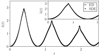
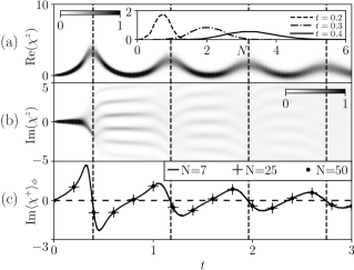
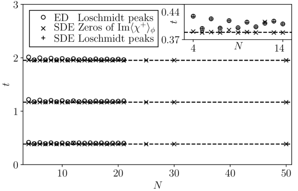
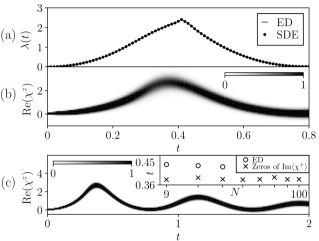
for unitary evolution in a non-zero transverse field. For quenches across a quantum critical point, $\lambda(t)$ is known to exhibit sharp peaks, corresponding to dynamical quantum phase transitions (DQPTs) in the thermodynamic limit Heyl et al. (2013); Karrasch and Schuricht (2013); Heyl (2014). Fig. 1 shows that the SDE method is able to resolve these peaks for a quantum quench across the critical point at $\Gamma_{c}=J/2$. The SDE results are in excellent agreement with exact diagonalization (ED) results obtained via the QuSpin package Weinberg and Bukov (2017). Remarkably, the presence of the DQPTs is reflected in the disentangling variables themselves. In Fig. 2 we plot the time evolution of the distribution of $\chi^{a}(t)\equiv N^{-1}\sum_{j}\xi_{j}^{a}(t)$ with $a=z$, as suggested by Eq. (11). It can be seen in Fig. 2(a) that both the average value and the width of the distribution of ${\rm Re}\,\chi^{z}(t)$ have smooth maxima in the vicinity of the DQPTs, as further illustrated in the inset. Likewise, ${\rm Im}\,\chi^{z}(t)$ shows pronounced signatures close to the DQPTs, as indicated in Fig. 2(b); these features become less visible with increasing $N$, and the overall phase of the argument of Eq. (11) becomes uniformly distributed over $[-\pi,\pi]$ due to its scaling with $N$. Further insight into the location of the DQPTs can be obtained from the SDEs. From Eq. (7) it can be seen that the turning points of ${\rm Re}\langle\chi^{z}(t)\rangle_{\phi}$ are determined by the zeros of ${\rm Im}\langle\chi^{+}(t)\rangle_{\phi}$ due to the exact relationship $\langle\dot{\chi}^{z}(t)\rangle_{\phi}=-i\Gamma\langle\chi^{+}(t)\rangle_{\phi}$ for the Ising SDEs. These zeros occur in close proximity to the DQPTs as shown in Figs. 2(c) and 3. The expectation values $\langle\chi^{z}(t)\rangle_{\phi}$ and $\langle\chi^{+}(t)\rangle_{\phi}$ and the characteristic times obtained from the classical distribution functions show strikingly little dependence on the system size, with results shown up to $N=50$. For comparison, we show the exact locations of the Loschmidt maxima obtained by averaging the complete exponential in Eq. (11), including both the real and imaginary parts of $\xi_{j}^{z}$ and their correlations; see inset of Fig. 3. The results are in very good agreement with ED.

Figure 2: Time-evolution of the distribution of $\chi^{z}(t)\equiv N^{-1}\sum_{j}\xi_{j}^{z}(t)$ for the quantum Ising model following a quantum quench from $\Gamma=0$ to $\Gamma=16\Gamma_{c}$ with $N=7$. (a) The distribution of ${\rm Re}\,\chi^{z}(t)$ shows smooth maxima and increased fluctuations in the vicinity of the Loschmidt peaks (dashed lines at $t=0.39$, $1.18$, $1.96$, $2.75$ obtained by ED). Inset: the average value and width of the distribution of ${\rm Re}\,\chi^{z}(t)$ increases on approaching the Loschmidt peaks as illustrated for the first peak. (b) The distribution of ${\rm Im}\,\chi^{z}(t)$ also shows signatures in the vicinity of the Loschmidt peaks. (c) Time-evolution of ${\rm Im}\langle\chi^{+}(t)\rangle_{\phi}$ for $N=7$, $25$, and $50$. The zeros of ${\rm Im}\langle\chi^{z}(t)\rangle_{\phi}$ occur in proximity to the turning points of $\lambda(t)$.

Figure 3: Characteristic times for the stationary points of ${\rm Re}\langle\chi^{z}(t)\rangle_{\phi}$ corresponding to the zeros of ${\rm Im}\langle\chi^{+}(t)\rangle_{\phi}$ following the quench considered in Fig. 2. The times are in close proximity to the Loschmidt peaks and have little dependence on $N$. Inset: Comparison of the Loschmidt peak times obtained from the SDE approach by averaging the complete exponential in Eq. (11), including its real and imaginary parts and their correlations, and ED for different system sizes.

Local Observables.— The stochastic approach can also be applied to other physical observables including the magnetization. Following a quench from an initial state $|\psi(0)\rangle$, the local magnetization evolves according to

$$\langle\hat{S}_{i}^{z}(t)\rangle=\langle\psi(0)|\hat{U}^{\dagger}(t)\hat{S}_{i}^{z}\hat{U}(t)|\psi(0)\rangle.$$ (12)

The forwards and backwards time-evolution operators can be decoupled by independent Hubbard–Stratonovich variables, $\phi_{i}^{a}$ and $\tilde{\phi}_{i}^{a}$, with corresponding disentangling variables $\xi_{i}^{a}(\phi)$ and $\tilde{\xi}_{i}^{a}(\tilde{\phi})$. For a quantum quench starting in the ferromagnetic ground state $|\psi(0)\rangle=\lvert\Downarrow\rangle$ with $\Gamma=0$, and time-evolving with $\Gamma\neq 0$, one obtains

$$\langle\hat{S}_{i}^{z}(t)\rangle=\bigg{\langle}f_{i}\left(\xi(t),\tilde{\xi}(t)\right)\bigg{\rangle}_{\phi,\tilde{\phi}},$$ (13)

where

$$f_{i}=-\frac{1}{2}e^{-\sum_{j}\tfrac{\xi_{j}^{z}+(\tilde{\xi}_{j}^{z})^{*}}{2}}[1-\xi_{i}^{+}(\tilde{\xi}_{i}^{+})^{*}]\prod_{j\neq i}[1+\xi_{j}^{+}(\tilde{\xi}_{j}^{+})^{*}].$$

In Fig. 4(a) we show the time-evolution of the magnetization $\mathcal{M}(t)=N^{-1}\sum\limits_{i=1}^{N}\langle\hat{S}_{i}^{z}(t)\rangle$ obtained from the stochastic average in Eq. (13). The results are in excellent agreement with ED for $N=3$. The use of smaller system sizes enables us to reach longer time-scales in the presence of two Hubbard–Stratonovich transformations. This allows us to verify that the time-integrated magnetization $\overline{\mathcal{M}}(t)=1/t\int_{0}^{t}\mathrm{d}s\,\mathcal{M}(s)$ (inset) approaches zero at late times as expected for the integrable Ising model in the absence of a longitudinal magnetic field Calabrese et al. (2011).

Figure 4: (a) Time-evolution of $\mathcal{M}(t)$ for the quantum Ising model following a quantum quench from $\Gamma=0$ to $\Gamma=16\,\Gamma_{c}$. The results obtained from the SDE (full circles) are in excellent agreement with ED (solid line) for $N=3$. Inset: the time-averaged magnetization $\overline{\mathcal{M}}(t)$ approaches zero at late times, as expected for the integrable case with $h=0$. The SDE results were obtained by averaging over $10^{6}$ realizations of the stochastic process with $dt=10^{-5}$. (b) $\mathcal{M}(t)$ for the non-integrable Ising model with $h=3J$, after a quench from $\Gamma=0$ to $\Gamma=2J$. The results obtained from the SDEs are in agreement with ED for $N=3$. Inset: the time-averaged magnetization $\overline{\mathcal{M}}(t)$ approaches the thermal value calculated via ED (dashed line) at late times, as expected for the non-integrable case. The SDE results were obtained by averaging over $10^{6}$ realizations of the stochastic process with $dt=10^{-5}$.

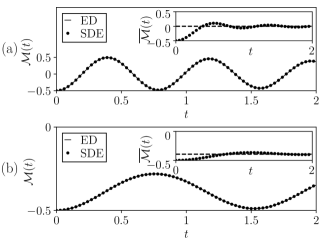
In Fig. 4(b) we show the dynamics of $\mathcal{M}(t)$ in the presence of a constant integrability-breaking longitudinal field $h$, so that $\hat{H}=\hat{H}_{\rm I}+h\sum_{j}\hat{S}^{z}_{j}$. We consider a quantum quench from the ferromagnetic ground state $\lvert\Downarrow\rangle$ with $\Gamma=0$ and $h=0$ to $\Gamma=2J$ and $h=3J$. Again, the results are in excellent agreement with ED. In this case, the time-averaged magnetization $\overline{\mathcal{M}}(t)$ approaches a non-vanishing expectation value as expected for the non-integrable Ising model with $h\neq 0$ Eisert et al. (2015). The asymptotic result is consistent with the thermal expectation value obtained via ED.

Higher Dimensions.— A remarkable feature of the stochastic approach is that it is not restricted to one-dimensional systems. To illustrate this we examine the quantum Ising model in $2+1$ dimensions:

$$\hat{H}_{\rm I}^{\mathrm{2D}}=-J\sum_{\langle\mathbf{i}\mathbf{j}\rangle}\hat{S}_{\mathbf{i}}^{z}\hat{S}_{\mathbf{j}}^{z}-\Gamma\sum_{\mathbf{i}}\hat{S}_{\mathbf{i}}^{x}.$$ (14)

In Fig. 5(a) we show $\lambda(t)$ following a quench from $\Gamma=0$ to $\Gamma=8J$, across the 2D quantum critical point at $\Gamma_{c}^{\mathrm{2D}}\sim 1.523J$ Pfeuty and Elliott (1971); du Croo de Jongh and van Leeuwen (1998). We initialize the system in the ferromagnetic ground state $\lvert\Downarrow\rangle$ and time evolve the 2D generalization of Eq. (11) using the SDEs in Eq. (8). The results are in excellent agreement with ED for a $3\times 5$ system. The 2D results in Fig. 5(a) show clear peaks in $\lambda(t)$, as found for coupled continuum chains and for classically tractable quenches from $\Gamma=\infty$ to $\Gamma=0$ James and Konik (2015); Heyl (2015). Here, however, the SDE results apply directly to the 2D quantum lattice model (14), without continuum approximations or assumptions of classical evolution. Moreover, the 2D DQPTs are signalled once again by the presence of enhanced fluctuations in the distribution of the disentangling variables, and the behavior of their classical averages; see Fig. 5(b). The dynamics of these variables can be tracked to larger system sizes as shown in Fig. 5(c) for a $10\times 10$ system. This provides a novel handle on the dynamics of higher-dimensional quantum many-body systems. As found in 1D, the time evolution of the classical average $\langle\chi^{z}\rangle_{\phi}$ and its turning points are strikingly independent of $N$. This, together with the form of Eq. (11), suggests the possibility of developing a classical large deviation approach to quantum dynamics in future work.

Figure 5: (a) Loschmidt rate function $\lambda(t)$ for the $2$D quantum Ising model following a quantum quench from $\Gamma=0$ to $\Gamma=8J$. The results obtained from the SDEs (filled circles) are in excellent agreement with ED (solid line) for a $3\times 5$ system. The results show sharp peaks in $\lambda(t)$ for quenches across the critical point at $\Gamma_{c}^{\rm 2D}\sim 1.523J$. The SDE results were obtained by averaging over $2.5\times 10^{7}$ stochastic realizations with $dt=10^{-5}$. (b) The corresponding distribution of ${\rm Re}\,\chi^{z}(t)$ for a $3\times 5$ system shows smooth maxima and increased fluctuations in the vicinity of the Loschmidt peaks. (c) Time-evolution of ${\rm Re}\,\chi^{z}(t)$ for a $10\times 10$ spin system showing additional turning points. Inset: comparison of exact times of the first Loschmidt peak (circles) and zeros of Im$\langle\chi^{+}\rangle$ (crosses) for square lattices of size up to $N=100$ spins.

Conclusions.— In this manuscript we have explored the dynamics of non-equilibrium quantum spin systems via an exact mapping to classical stochastic processes. We have shown that this approach can handle the dynamics of integrable and non-integrable systems, including those in higher dimensions. This novel approach provides a valuable handle on challenging problems out of equilibrium and provides fundamental links between quantum and classical dynamics. There are many directions for future research including comparison with tensor network and machine learning approaches, and the development of enhanced numerical sampling techniques for the SDEs.

Acknowledgements.— We acknowledge helpful conversations with Samuel Begg, George Booth, Andrew Green, Vladimir Gritsev and Lev Kantorovich. MJB is indebted to John Chalker for early discussions on the Hubbard–Stratonovich and stochastic approaches to quantum dynamics. SD acknowledges funding from the EPSRC Centre for Doctoral Training in Cross-Disciplinary Approaches to Non-Equilibrium Systems (CANES) under grant EP/L015854/1. MJB, BD and SD thank the Centre for Non-Equilibrium Science (CNES) and the Thomas Young Centre (TYC). We are grateful to the UK Materials and Molecular Modelling Hub for computational resources, which is partially funded by EPSRC (EP/P020194/1). We acknowledge computer time on the Rosalind High Performance Computer Cluster.

References

- Kinoshita et al. (2006) T. Kinoshita, T. Wenger, and D. S. Weiss, Nature 440, 900 (2006).
- Langen et al. (2015a) T. Langen, S. Erne, R. Geiger, B. Rauer, T. Schweigler, M. Kuhnert, W. Rohringer, I. E. Mazets, T. Gasenzer, and J. Schmiedmayer, Science 348, 207 (2015a).
- Lamporesi et al. (2013) G. Lamporesi, S. Donadello, S. Serafini, F. Dalfovo, and G. Ferrari, Nat. Phys. 9, 656 (2013).
- Weiler et al. (2008) C. N. Weiler, T. W. Neely, D. R. Scherer, A. S. Bradley, M. J. Davis, and B. P. Anderson, Nature 455, 948 (2008).
- Weitenberg et al. (2011) C. Weitenberg, M. Endres, J. F. Sherson, M. Cheneau, P. Schausz, T. Fukuhara, I. Bloch, and S. Kuhr, Nature 471, 319 (2011).
- Bakr et al. (2010) W. S. Bakr, A. Peng, M. E. Tai, R. Ma, J. Simon, J. I. Gillen, S. Fölling, L. Pollet, and M. Greiner, Science 329, 547 (2010).
- Langen et al. (2015b) T. Langen, R. Geiger, and J. Schmiedmayer, Annu. Rev. Condens. Matter Phys. 6, 201 (2015b).
- Eisert et al. (2015) J. Eisert, M. Friesdorf, and C. Gogolin, Nat. Phys. 11, 124 (2015).
- Deutsch (1991) J. M. Deutsch, Phys. Rev. A 43, 2046 (1991).
- Srednicki (1994) M. Srednicki, Phys. Rev. E 50, 888 (1994).
- Rigol et al. (2008) M. Rigol, V. Dunjko, and M. Olshanii, Nature 452, 854 (2008).
- Cramer et al. (2008) M. Cramer, C. M. Dawson, J. Eisert, and T. J. Osborne, Phys. Rev. Lett. 100, 030602 (2008).
- Calabrese and Cardy (2007) P. Calabrese and J. Cardy, J. Stat. Mech. Theor. Exp. 2007, P10004 (2007).
- Rigol et al. (2007) M. Rigol, V. Dunjko, V. Yurovsky, and M. Olshanii, Phys. Rev. Lett. 98, 050405 (2007).
- Polkovnikov et al. (2011) A. Polkovnikov, K. Sengupta, A. Silva, and M. Vengalattore, Rev. Mod. Phys. 83, 863 (2011).
- Gogolin and Eisert (2016) C. Gogolin and J. Eisert, Rep. Prog. Phys. 79, 056001 (2016).
- Essler and Fagotti (2016) F. H. L. Essler and M. Fagotti, J. Stat. Mech. Theor. Exp. 2016, 064002 (2016).
- Bhaseen et al. (2015) M. J. Bhaseen, B. Doyon, A. Lucas, and K. Schalm, Nat. Phys. 11, 509 (2015).
- Doyon et al. (2015) B. Doyon, A. Lucas, K. Schalm, and M. J. Bhaseen, J. Phys. A: Math. Theor. 48, 095002 (2015).
- Bernard and Doyon (2016) D. Bernard and B. Doyon, J. Stat. Mech. Theor. Exp. 2016, 033104 (2016).
- Castro-Alvaredo et al. (2016) O. A. Castro-Alvaredo, B. Doyon, and T. Yoshimura, Phys. Rev. X 6, 041065 (2016).
- Carleo and Troyer (2017) G. Carleo and M. Troyer, Science 355, 602 (2017).
- Schmitt and Heyl (2018) M. Schmitt and M. Heyl, SciPost Phys. 4, 013 (2018).
- Hogan and Chalker (2004) P. M. Hogan and J. T. Chalker, J. Phys. A: Math. Gen. 37, 11751 (2004).
- Galitski (2011) V. Galitski, Phys. Rev. A 84, 012118 (2011).
- Ringel and Gritsev (2013) M. Ringel and V. Gritsev, Phys. Rev. A 88, 062105 (2013).
- Hubbard (1959) J. Hubbard, Phys. Rev. Lett. 3, 77 (1959).
- Stratonovich (1957) R. L. Stratonovich, Sov. Phys. Dokl. 2, 416 (1957).
- Wei and Norman (1963) J. Wei and E. Norman, J. Math. Phys. 4, 575 (1963).
- Kolokolov (1986) I. Kolokolov, Phys. Lett. A 114, 99 (1986).
- Kloeden and Platen (1992) P. E. Kloeden and E. Platen, Numerical Solution of Stochastic Differential Equations (Springer, 1992).
- Note (1) In order to diagonalize the action (4), the matrix should be symmetric and invertible. For system sizes that are multiples of we add a constant to to eliminate zero eigenvalues. This modifies the evolution of the stochastic variables but does not influence physical observables.
- Hutzenthaler et al. (2011) M. Hutzenthaler, A. Jentzen, and P. E. Kloeden, Proc. Royal Soc. Lond. A 467, 1563 (2011).
- Heyl et al. (2013) M. Heyl, A. Polkovnikov, and S. Kehrein, Phys. Rev. Lett. 110, 135704 (2013).
- Karrasch and Schuricht (2013) C. Karrasch and D. Schuricht, Phys. Rev. B 87, 195104 (2013).
- Heyl (2014) M. Heyl, Phys. Rev. Lett. 113, 205701 (2014).
- Weinberg and Bukov (2017) P. Weinberg and M. Bukov, SciPost Phys. 2, 003 (2017).
- Calabrese et al. (2011) P. Calabrese, F. H. L. Essler, and M. Fagotti, Phys. Rev. Lett. 106, 227203 (2011).
- Pfeuty and Elliott (1971) P. Pfeuty and R. J. Elliott, J. Phys. C: Solid State Phys. 4, 2370 (1971).
- du Croo de Jongh and van Leeuwen (1998) M. S. L. du Croo de Jongh and J. M. J. van Leeuwen, Phys. Rev. B 57, 8494 (1998).
- James and Konik (2015) A. J. A. James and R. M. Konik, Phys. Rev. B 92, 161111 (2015).
- Heyl (2015) M. Heyl, Phys. Rev. Lett. 115, 140602 (2015).