Agreement Rate Initialized Maximum Likelihood Estimator for Ensemble Classifier Aggregation and Its Application in Brain-Computer Interface

Abstract

Ensemble learning is a powerful approach to construct a strong learner from multiple base learners. The most popular way to aggregate an ensemble of classifiers is majority voting, which assigns a sample to the class that most base classifiers vote for. However, improved performance can be obtained by assigning weights to the base classifiers according to their accuracy. This paper proposes an agreement rate initialized maximum likelihood estimator (ARIMLE) to optimally fuse the base classifiers. ARIMLE first uses a simplified agreement rate method to estimate the classification accuracy of each base classifier from the unlabeled samples, then employs the accuracies to initialize a maximum likelihood estimator (MLE), and finally uses the expectation-maximization algorithm to refine the MLE. Extensive experiments on visually evoked potential classification in a brain-computer interface application show that ARIMLE outperforms majority voting, and also achieves better or comparable performance with several other state-of-the-art classifier combination approaches.

I Introduction

Ensemble learning [4, 2, 7] is very effective in constructing a strong learner from multiple base (weak) learners, for both classification and regression problems. This paper focuses on ensemble learning for binary classification problems. More specifically, we investigate how to optimally combine multiple base binary classifiers for better performance.

Given an ensemble of base binary classifiers, the simplest yet most popular ensemble learning approach is majority voting (MV), i.e., assigning a sample to the class that most base classifiers agree on. However, the base classifiers usually have different classification accuracies, and hence considering them equally (as in MV) in aggregation may not be optimal. It is more intuitive to use weighted voting, where the weight is a function of the corresponding classification accuracy.

The first step in weighted voting is to estimate the accuracies of the base classifiers. There could be two approaches. The first is to use cross-validation on the training data. However, in many applications the training data may be very limited, so the cross-validation accuracy may not be reliable. For example, in the brain-computer interface (BCI) system calibration application considered in this paper (Section III), to increase the utility of the BCI system, we would like to use as little calibration data as possible, preferably zero; so, it is difficult to perform cross-validation. Moreover, in certain situations only the output of the classifiers are available. Thus, it is not feasible to perform cross-validation.

Because of these limitations, in this paper we consider the second approach, in which the accuracies of the base classifiers are estimated from their predictions on the unlabeled samples. There have been a few studies in this direction. Platanios et al. [12] used agreement rate (AR) among different base classifiers to estimate both the marginal and joint error rates (However, they did not show how the error rates can be used to optimally combine the classifiers). Parisi et al. [11] proposed a spectral meta-learner (SML) approach to estimate the accuracies of the base classifiers from their population covariance matrix, and then used them in a maximum likelihood estimator (MLE) to aggregate these base classifiers. Researchers from the same group then proposed several different approaches [9, 8, 16] to improve the SML. They have all shown better performance than MV.

This paper proposes a new classifier combination approach, agreement rate initialized maximum likelihood estimator (ARIMLE), to aggregate the base classifiers. As its name suggests, it first uses the AR method to estimate the classifier accuracies, and then employs them in an MLE to optimally fuse the classifiers. Using a visually evoked potential (VEP) BCI experiment with 14 subjects and three different EEG headsets, we show that ARIMLE outperforms MV, and its performance is also better than or comparable to several other state-of-the-art classifier combination approaches.

The remainder of the paper is organized as follows: Section II introduces the details of the ARIMLE algorithm. Section III describes experiment setup and performance comparisons of eight different algorithms. Section IV draws conclusions.

II ARIMLE for Classifier Aggregation

This section introduces the proposed ARIMLE for classifier aggregation.

II-A Problem Setup

The problem setup is very similar to that in [11, 9, 8, 16], so we use similar notations and terminology.

We consider binary classification problems with input space $\mathcal{X}$ and output space $\mathcal{Y}\in\{-1,1\}$. A sample and class label pair $(X,Y)\in\mathcal{X}\times\mathcal{Y}$ is a random vector with joint probability density function $p(\mathbf{x},y)$, and marginal probability density functions $p_{X}(\mathbf{x})$ and $p_{Y}(y)$. Assume there are $n$ unlabeled samples, $\{\mathbf{x}_{j}\}_{j=1}^{n}$, with unknown true labels $\{y_{j}\}_{j=1}^{n}$. Assume also there are $m$ base binary classifiers, $\{f_{i}\}_{i=1}^{m}$, and the $i$th classifier’s prediction for $\mathbf{x}_{j}$ is $f_{i}(\mathbf{x}_{j})$. Define the classification sensitivity of $f_{i}$ as

$$\psi_{i}=\mathrm{P}(f_{i}(X)=1|Y=1)$$ (1)

and its specificity as

$$\eta_{i}=\mathrm{P}(f_{i}(X)=-1|Y=-1)$$ (2)

Then, the balanced classification accuracy (BCA) of $f_{i}$ is

$$\pi_{i}=\frac{1}{2}(\psi_{i}+\eta_{i}).$$ (3)

As in [11], we make two important assumptions in the following derivation: 1) The $n$ unlabeled samples $\{\mathbf{x}_{j}\}_{j=1}^{n}$ are independent and identically distributed realizations from $p_{X}(\mathbf{x})$; and, 2) The $m$ base binary classifiers $\{f_{i}\}_{i=1}^{m}$ are independent, i.e., prediction errors made by one classifier are independent of those made by any other classifier.

II-B Agreement Rate (AR) Computation

The AR method presented in this subsection is a simplified version of the one introduced in [12], by assuming any pair of $f_{i_{1}}$ and $f_{i_{2}}$ ($i_{1}\neq i_{2}$) are independent. It is used to compute the (unbalanced) error rate of each classifier, which is defined as

$$e_{i}=\mathrm{P}(f_{i}(X)\neq Y),\quad i=1,...,m$$ (4)

which is in turn used in the next subsection to construct the MLE.

We define the AR of two classifiers $f_{i_{1}}$ and $f_{i_{2}}$ $(i_{1}\neq i_{2}$) as the probability that they give identical outputs, i.e.,

$$a_{i_{1},i_{2}}=\mathrm{P}(f_{i_{1}}(X)=f_{i_{2}}(X))$$ (5)

which can be empirically computed from the predictions of the two classifiers.

As in [12], we can show that

$$a_{i_{1},i_{2}}=1-e_{i_{1}}-e_{i_{2}}+2e_{i_{1},i_{2}}$$ (6)

where $e_{i_{1},i_{2}}$ is the (unbalanced) joint error rate of $f_{i_{1}}$ and $f_{i_{2}}$. Under the assumption that $f_{i_{1}}$ and $f_{i_{2}}$ are independent, we have $e_{i_{1},i_{2}}=e_{i_{1}}\cdot e_{i_{2}}$, and hence (6) can be re-expressed as:

$$a_{i_{1},i_{2}}=1-e_{i_{1}}-e_{i_{2}}+2e_{i_{1}}\cdot e_{i_{2}}$$ (7)

To find the $m$ error rates for the $m$ classifiers, we compute the AR $a_{i_{1},i_{2}}$ for all $\frac{1}{2}m(m-1)$ possible combinations of $(i_{1},i_{2})$, $i_{1}=1,...,m$, $i_{2}=1,...,m$, and $i_{1}\neq i_{2}$. By substituting them into (7), we have $\frac{1}{2}m(m-1)$ equations and $m$ variables $\{e_{i}\}_{i=1}^{m}\in[0,1]$, which can be easily solved by a constrained optimization routine, e.g., fmincon in Matlab.

The main difference between our approach for estimating $\{e_{i}\}_{i=1}^{m}$ and the one in [12] is that, [12] considers the general case that different base classifiers are inter-dependent, and hence it tries to find $2^{m}-1$ error rates ($m$ marginal error rates $\{e_{i}\}_{i=1}^{m}$ for the individual classifiers, $\frac{1}{2}m(m-1)$ joint error rates $\{e_{i_{1},i_{2}}\}_{i_{1}\neq i_{2}}$ for all pairs of classifiers, $\frac{1}{6}m(m-1)(m-2)$ joint error rates $\{e_{i_{1},i_{2},i_{3}}\}_{i_{1}\neq i_{2}\neq i_{3}}$ for all 3-tuples of classifiers, and so on) all at once. Since there are more error rates than equations, it introduces additional constraints, e.g., to minimize the dependence between different classifiers, to solve for the $2^{m}-1$ error rates. We do not adopt that approach because of its high computational cost. For example, in our experiments in Section III we have 13 base classifiers, i.e., $m=13$, and hence $2^{m}-1=8191$ error rates to optimize, which is very computationally expensive. So, we make the simplified assumption that all $m$ base classifiers are independent, and hence only need to find the $m$ marginal error rates $\{e_{i}\}_{i=1}^{m}$. $\{e_{i}\}_{i=1}^{m}$ estimated here may not be as accurate as the ones in [12], but they are only used to initialize our MLE, and in the next subsection we shall use an expectation-maximization (EM) algorithm to iteratively improve them.

Once $\{e_{i}\}_{i=1}^{m}$ are obtained, the (unbalanced) classification accuracy of $f_{i}$ is then computed as $1-e_{i}$, which is also an estimate of the BCA $\pi_{i}$, i.e.,

$$\pi_{i}\approx 1-e_{i},\quad i=1,...,m$$ (8)

by assuming that the positive and negative classes have similar accuracies.

II-C Maximum Likelihood Estimator (MLE)

As shown in [11], the MLE from $\{f_{i}\}_{i=1}^{m}$ is

$$\hat{y}=\mathrm{sign}\left[\sum_{i=1}^{m}\left(f_{i}(\mathbf{x})\ln\alpha_{i}+\ln\beta_{i}\right)\right]$$ (9)

where

$$\alpha_{i} =\frac{\psi_{i}\eta_{i}}{(1-\psi_{i})(1-\eta_{i})}$$ (10)

$$\beta_{i} =\frac{\psi_{i}(1-\psi_{i})}{\eta_{i}(1-\eta_{i})}$$ (11)

i.e., the MLE is a linear ensemble classifier, whose weights depend on the unknown specificities and sensitivities of the $m$ base classifiers.

The classical approach for solving (9) is to jointly maximize the likelihood for all $\{\hat{y}_{j}\}_{j=1}^{n}$, $\{\psi_{i}\}_{i=1}^{m}$ and $\{\eta_{i}\}_{i=1}^{m}$ using an EM algorithm [10, 13, 11, 20, 17, 21], which first estimates $\{\psi_{i}\}_{i=1}^{m}$ and $\{\eta_{i}\}_{i=1}^{m}$ given some initial $\{\hat{y}_{j}\}_{j=1}^{n}$, and then updates $\{\hat{y}_{j}\}_{j=1}^{n}$ using the newly estimated $\{\psi_{i}\}_{i=1}^{m}$ and $\{\eta_{i}\}_{i=1}^{m}$, and iterates until they converge. The question is how to find a good initial estimate of $\{\hat{y}_{j}\}_{j=1}^{n}$ so that the final estimates are less likely to be trapped in a local minimum.

We solve this problem by using the results from [11], which suggested that the BCAs $\{\pi_{i}\}_{i=1}^{m}$ can be used to compute a good initialization of $\{\hat{y}_{j}\}_{j=1}^{n}$, i.e.,

$$\hat{y}_{j}=\mathrm{sign}\left[\frac{\sum_{i=1}^{m}(2\pi_{i}-1)f_{i}(\mathbf{x}_{j})}{\sum_{i=1}^{m}(2\pi_{i}-1)}\right],\quad j=1,...,n$$ (12)

The EM algorithm can then run from there.

II-D The Complete ARIMLE Algorithm

The complete ARIMLE algorithm is shown in Algorithm 1. It first uses AR to compute the error rate of each base classifier, then employs the error rates to initialize the EM algorithm, and finally runs the EM algorithm until a stopping criterion is met, which could be reaching the maximum number of iterations, or the difference between the last two iterations is smaller than a certain threshold. The former is used in this paper.

Input: $n$ unlabeled samples, $\{\mathbf{x}_{j}\}_{j=1}^{n}$;

          $m$ base binary classifiers, $\{f_{i}\}_{i=1}^{m}$.

Output: The maximum likelihood estimates $\{\hat{y}\}_{j=1}^{n}$.

for $i_{1}=1,...,m-1$ do

       for $i_{2}=i_{1}+1,...,m$ do

             Compute $a_{i_{1},i_{2}}$ in (5);

            

       end for

      Solve for $\{e_{i}\}_{i=1}^{m}$ in (7) using constrained optimization;

       Compute $\{\pi_{i}\}_{i=1}^{m}$ using (8);

      

end for

Initialize $\{\hat{y}_{j}\}_{j=1}^{n}$ using (12);

while stopping criterion not met do

       Compute $\{\psi_{i}\}_{i=1}^{m}$ in (1) and $\{\eta_{i}\}_{i=1}^{m}$ in (2), by treating $\{\hat{y}_{j}\}_{j=1}^{n}$ as the true labels;

       Compute $\{\alpha_{i}\}_{i=1}^{m}$ in (10) and $\{\beta_{i}\}_{i=1}^{m}$ in (11);

       Update $\{\hat{y}_{j}\}_{j=1}^{n}$ using (9);

      

end while

Return The latest $\{\hat{y}_{j}\}_{j=1}^{n}$.

Algorithm 1 The ARIMLE algorithm.

III Experiments and Analysis

This section presents the experiment setup that is used to evaluate the performance of ARIMLE, and the performance comparison of ARIMLE with MV and several other state-of-the-art classifier combination approaches.

III-A Experiment Setup

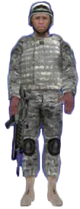
We used data from a VEP oddball task [14]. Image stimuli of an enemy combatant [target, as shown in Fig. 1] or a U.S. Soldier [non-target, as shown in Fig. 1] were presented to subjects at a rate of 0.5 Hz. The subjects were instructed to identify each image as being target or non-target with a unique button press as quickly and accurately as possible. There were a total of 270 images, of which 34 were targets. The experiments were approved by the U.S. Army Research Laboratory (ARL) Institutional Review Board (Protocol # 20098-10027). The voluntary, fully informed consent of the persons used in this research was obtained as required by federal and Army regulations [19, 18]. The investigator adhered to Army policies for the protection of human subjects.

Figure 1: Example images of (a) a target; (b) a non-target.

Eighteen subjects participated in the experiments, which lasted on average 15 minutes. Data from four subjects were not used due to data corruption or lack of responses. Signals from each subject were recorded with three different EEG headsets, including a wired 64-channel 512Hz ActiveTwo system from BioSemi, a wireless 9-channel 256Hz B-Alert X10 EEG Headset System from Advanced Brain Monitoring (ABM), and a wireless 14-channel 128Hz EPOC headset from Emotiv.

III-B Preprocessing and Feature Extraction

The EEG data preprocessing and feature extraction methods were similar to those used in [23, 24]. EEGLAB [3] were used to extract raw EEG amplitude features.

For each headset, we first band-passed the EEG signals to [1, 50] Hz, then downsampled them to 64 Hz, performed average reference, and next epoched them to the $[0,0.7]$ second interval timelocked to stimulus onset. We removed mean baseline from each channel in each epoch and removed epochs with incorrect button press responses. The final numbers of epochs from the 14 subjects are shown in Table I. Observe that there is significant class imbalance for all headsets.

TABLE I: Number of epochs for each subject after preprocessing. The numbers of target epochs are given in the parentheses.

Subject	1	2	3	4	5	6	7	8	9	10	11	12	13	14
BioSemi	241(26)	260(24)	257(24)	261(29)	259(29)	264(30)	261(29)	252(22)	261(26)	259(29)	267(32)	259(24)	261(25)	269(33)
Emotiv	263(28)	265(30)	266(30)	255(23)	264(30)	263(32)	266(30)	252(22)	261(26)	266(29)	266(32)	264(33)	261(26)	267(31)
ABM	270(34)	270(34)	235(30)	270(34)	270(34)	270(34)	270(34)	270(33)	270(34)	239(30)	270(34)	270(34)	251(31)	270(34)

Each [0, 0.7] second epoch contains 45 raw EEG magnitude samples. The concatenated feature vector has hundreds of dimensions. To reduce the dimensionality, we performed a simple principal component analysis, and took only the scores for the first 20 principal components. We then normalized each feature dimension separately to $[0,1]$ for each subject.

III-C Evaluation Process and Performance Measures

Although we knew the labels of all EEG epochs from all headsets for each subject, we simulated a different scenario, as shown in Fig. 2: None of the epochs from the current subject under study was initially labeled, but all epochs from all the other 13 subjects with the same headset were labeled. Our approach was to iteratively label some epochs from the current subject, and then to build an ensemble of 13 classifiers (one from each of the 13 auxiliary subjects) to label the rest of the epochs. Seven different algorithms (see the next subsection), including ARIMLE, were used to the aggregate the 13 classifiers. The goal was to achieve the highest BCA for the new subject, with as few labeled epochs as possible. Each classifier in the ensemble was constructed using the weighted adaptation regularization (wAR) algorithm in [24], which is a domain adaptation approach in transfer learning.

In each iteration five epochs were labeled, and the algorithm terminated after 20 iterations, i.e., after 100 epochs were labeled. We repeated this process 30 times for each subject and each headset so that statistically meaningful results could be obtained.

The BCA was used as our performance measure.

Figure 2: Flowchart of the evaluation process.

III-D Algorithms

We compare our propose ARIMLE with a baseline algorithm and several other state-of-the-art classifier combination approaches in the literature:

1. Baseline (BL), which uses only available labeled subject-specific data to train a support vector machine classifier and then applies it to the remaining unlabeled data.

2. MV, which computes the final label as $\hat{y}_{j}=\mathrm{sign}\left[\sum_{i=1}^{m}f_{i}(\mathbf{x}_{j})\right]$, $j=1,...,n$. This is the most popular and also the simplest ensemble combination approach in the literature and practice.

3. Spectral meta-learner (SML) [11], which estimates the BCAs of the base classifiers from their population covariance matrix, and then uses them in (12) to compute the final estimates. There is no iterative EM algorithm involved.

4. Iterative MLE (iMLE) [11], which performs the above SML first and then uses an EM algorithm to refine the MLE.

5. Improved SML (i-SML) [9], which first estimates the class imbalance of the labels and then uses that to directly estimate the sensitivity and specificity of each base classifier. The sensitivities and specificities are then used to construct the MLE.

6. Latent SML (L-SML) [8], which, instead of assuming all $m$ classifiers are conditionally independent, assumes the $m$ classifiers can be partitioned into several groups according to a latent variable: the classifiers in the same group can be correlated, but the classifiers from different groups are conditionally independent. It is hoped that in this way it can better handle correlated base classifiers.

Additionally, we also constructed an oracle SML (O-SML), which assumes that we know the true sensitivity and specificity of each base classifier, to represent the upper bound of the classification performance we could get from these $m$ base classifiers using MLE.

III-E Experimental Results and Discussions

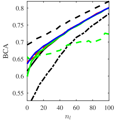
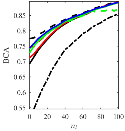
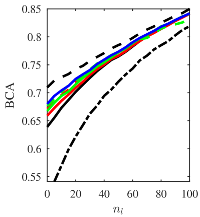
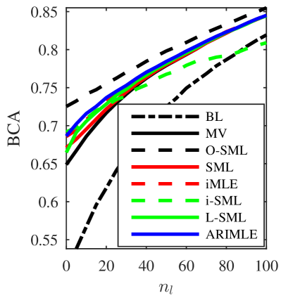
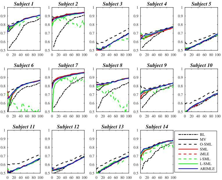
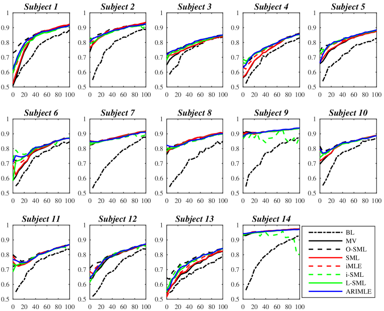
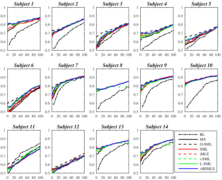
The average BCAs of the eight algorithms across the 14 subjects and three EEG headsets are shown in Fig. 3, along with the average performances across the three headsets, where $n_{l}$ denotes the number of labeled samples from the new subject. The accuracies for each individual subject, averaged over 30 runs, are shown in Fig. 4. Non-parametric multiple comparison tests using Dunn’s procedure [5, 6] were also performed on the combined data from all the subjects and headsets to determine if the difference between any pair of algorithms was statistically significant, with a $p$-value correction using the False Discovery Rate method by [1]. The results are shown in Table II, with the statistically significant ones marked in bold. Observe that:

Figure 3: Average BCAs of the eight algorithms across the 14 subjects. (a) ABM headset; (b) BioSemi headset; (c) Emotiv headset; (d) average of the three headsets.

1. ARIMLE had significantly better performance than BL, which did not use transfer learning and ensemble learning. In fact, almost all seven algorithms based on transfer learning and ensemble learning achieved much better performance than BL.

2. ARIMLE almost always outperformed MV, SML and L-SML, and the performance improvement was statistically significant for small $n_{l}$.

3. ARIMLE had comparable performance with iMLE. For small $n_{l}$, the BCA of ARIMLE was slightly higher than iMLE. The performance difference was not statistically significant, but very close to the threshold.

4. i-SML gave good performance for most subjects, but sometimes the predictions were significantly off-target. Overall, ARIMLE outperformed i-SML.

5. O-SML outperformed ARIMLE, and the performance difference was statistically significant when $n_{l}$ is small, which suggests that there is still room for ARIMLE to improve: if the sensitivity and specificity of the base binary classifiers can be better estimated, then the performance of ARIMLE could further approach O-SML. This is one of our future research directions.

In summary, we have shown through extensive experiments that ARIMLE significantly outperformed MV, and its performance was also better than or comparable to several state-of-the-art classifier combination approaches. Although a BCI application was considered in this paper, we believe the applicability of ARIMLE is far beyond that.

Figure 4: Individual BCAs of the eight algorithms for the 14 subjects, averaged over 30 runs for each headset. (a) ABM headset; (b) BioSemi headset; (c) Emotiv headset. Horizontal axis: $n_{l}$, the number of labeled epochs from the subject. Vertical axis: BCA.

TABLE II: $p$-values of non-parametric multiple comparisons of the BCA of ARIMLE versus other seven algorithms.

$n_{l}$	BL	MV	O-SML	SML	iMLE	i-SML	L-SML
0	N/A	.0000	.0000	.0009	.4750	.0698	.0000
5	.0000	.0000	.0000	.0000	.0466	.4565	.0266
10	.0000	.0000	.0000	.0000	.0546	.2410	.0191
15	.0000	.0000	.0001	.0001	.0832	.3063	.0550
20	.0000	.0000	.0005	.0010	.1683	.1470	.0460
25	.0000	.0011	.0015	.0083	.2398	.1684	.1306
30	.0000	.0202	.0014	.0645	.4245	.1412	.1735
35	.0000	.0428	.0080	.1026	.3781	.1436	.2437
40	.0000	.0801	.0163	.1228	.3734	.0847	.2150
45	.0000	.1546	.0117	.2214	.4656	.1121	.3344
50	.0000	.2126	.0105	.2581	.4386	.0370	.2503
55	.0000	.2340	.0199	.2528	.4816	.0352	.3380
60	.0000	.2707	.0359	.2972	.4650	.0291	.3073
65	.0000	.3110	.0331	.3107	.4908	.0306	.3201
70	.0000	.4088	.0263	.4222	.4682	.0091	.4287
75	.0000	.4815	.0403	.4418	.4777	.0028	.4046
80	.0000	.5060	.0355	.5442	.4582	.0008	.5331
85	.0000	.4985	.0336	.4813	.4857	.0004	.4733
90	.0000	.4706	.0434	.4885	.4522	.0002	.4625
95	.0000	.5057	.0690	.4978	.5165	.0001	.5367
100	.0000	.4674	.0436	.4842	.4792	.0000	.4890

IV Conclusions

This paper has proposed an ARIMLE approach to optimally aggregate multiple base binary classifiers in ensemble learning. It first uses AR to estimate the classification accuracies of the base classifiers from the unlabeled samples, which are then used to initialize an MLE. An EM algorithm is then employed to refine the MLE. Extensive experiments on visually evoked potential classification in a BCI application, which involved 14 subjects and three different EEG headsets, showed that ARIMLE significantly outperformed MV, and its performance was also better than or comparable to several other state-of-the-art classifier combination approaches. We expect ARIMLE to have broad applications beyond BCI.

Our future research will investigate the integration of ARIMLE with other machine learning approaches for more performance improvement. We have shown in [22, 23] that active learning [15] can be combined with transfer learning to improve the offline classification performance: active learning optimally selects the most informative unlabeled samples to label (rather than random sampling), and transfer learning combines subject-specific samples with labeled samples from similar/relevant tasks to build better base classifiers. ARIMLE is an optimal classifier combination approach, which is independent of and also complementary to active learning and transfer learning, so it can be combined with them for further improved performance. We have used ARIMLE to combine base classifiers constructed by transfer learning in this paper, and will integrate them with active learning in the future.

References

- [1] Y. Benjamini and Y. Hochberg, “Controlling the false discovery rate: A practical and powerful approach to multiple testing,” Journal of the Royal Statistical Society, Series B (Methodological), vol. 57, pp. 289–300, 1995.
- [2] L. Breiman, “Arcing classifier (with discussion and a rejoinder by the author),” The Annals of Statistics, vol. 26, no. 3, pp. 801–849, 1998.
- [3] A. Delorme and S. Makeig, “EEGLAB: an open source toolbox for analysis of single-trial EEG dynamics including independent component analysis,” Journal of Neuroscience Methods, vol. 134, pp. 9–21, 2004.
- [4] T. G. Dietterich, “Ensemble methods in machine learning,” in Proc. 1st Int’l Workshop on Multiple Classifier Systems, Cagliari, Italy, July 2000, pp. 1–15.
- [5] O. Dunn, “Multiple comparisons among means,” Journal of the American Statistical Association, vol. 56, pp. 62–64, 1961.
- [6] O. Dunn, “Multiple comparisons using rank sums,” Technometrics, vol. 6, pp. 214–252, 1964.
- [7] S. Hashem, “Optimal linear combinations of neural networks,” Neural Networks, vol. 10, no. 4, pp. 599–614, 1997.
- [8] A. Jaffe, E. Fetaya, B. Nadler, T. Jiang, and Y. Kluger, “Unsupervised ensemble learning with dependent classifiers,” arXiv: 1510.05830, 2015.
- [9] A. Jaffe, B. Nadler, , and Y. Kluger, “Estimating the accuracies of multiple classifiers without labeled data,” in Proc. 18th Int’l Conf. on Artificial Intelligence and Statistics (AISTATS), San Diego, CA, May 2015.
- [10] D. A. P. and S. A. M., “Maximum likelihood estimation of observer error-rates using the EM algorithm,” Applied Statistics, vol. 28, no. 1, pp. 20–28, 1979.
- [11] F. Parisi, F. Strino, B. Nadler, and Y. Kluger, “Ranking and combining multiple predictors without labeled data,” Proc. National Academy of Science, vol. 111, no. 4, pp. 1253–1258, 2014.
- [12] E. A. Platanios, A. Blum, and T. M. Mitchell, “Estimating Accuracy from Unlabeled Data,” in Proc. Int’l. Conf. on Uncertainty in Artificial Intelligence (UAI), Quebec, Canada, July 2014, pp. 1–10.
- [13] V. C. Raykar, S. Yu, L. H. Zhao, G. H. Valadez, C. Florin, L. Bogoni, and L. Moy, “Learning from crowds,” Journal of Machine Learning Research, vol. 11, pp. 1297–1322, 2010.
- [14] A. J. Ries, J. Touryan, J. Vettel, K. McDowell, and W. D. Hairston, “A comparison of electroencephalography signals acquired from conventional and mobile systems,” Journal of Neuroscience and Neuroengineering, vol. 3, no. 1, pp. 10–20, 2014.
- [15] B. Settles, “Active learning literature survey,” University of Wisconsin–Madison, Computer Sciences Technical Report 1648, 2009.
- [16] U. Shaham, X. Cheng, O. Dror, A. Jaffe, B. Nadler, J. Chang, and Y. Kluger, “A deep learning approach to unsupervised ensemble learning,” ArXiv: 1602.02285, 2016.
- [17] V. S. Sheng, F. Provost, and P. G. Ipeirotis, “Get another label? improving data quality and data mining using multiple, noisy labelers,” in Proc. 14th ACM SIGKDD Int’l Conf. on Knowledge Discovery and Data Mining, Las Vegas, NV, August 2008, pp. 614–622.
- [18] US Department of Defense Office of the Secretary of Defense, “Code of federal regulations protection of human subjects,” Government Printing Office, no. 32 CFR 19, 1999.
- [19] US Department of the Army, “Use of volunteers as subjects of research,” Government Printing Office, no. AR 70-25, 1990.
- [20] P. Welinder, S. Branson, P. Perona, and S. J. Belongie, “The multidimensional wisdom of crowds,” in Advances in Neural Information Processing Systems 23, J. Lafferty, C. Williams, J. Shawe-taylor, R. Zemel, and A. Culotta, Eds., 2010, pp. 2424–2432.
- [21] J. Whitehill, T. fan Wu, J. Bergsma, J. R. Movellan, and P. L. Ruvolo, “Whose vote should count more: Optimal integration of labels from labelers of unknown expertise,” in Proc. Advances in Neural Information Processing Systems (NIPS), Vancouver, Canada, December 2009, pp. 2035–2043.
- [22] D. Wu, B. J. Lance, and V. J. Lawhern, “Active transfer learning for reducing calibration data in single-trial classification of visually-evoked potentials,” in Proc. IEEE Int’l Conf. on Systems, Man, and Cybernetics, San Diego, CA, October 2014.
- [23] D. Wu, V. J. Lawhern, W. D. Hairston, and B. J. Lance, “Switching EEG headsets made easy: Reducing offline calibration effort using active weighted adaptation regularization,” IEEE Trans. on Neural Systems and Rehabilitation Engineering, vol. 24, no. 11, pp. 1125–1137, 2016.
- [24] D. Wu, V. J. Lawhern, and B. J. Lance, “Reducing offline BCI calibration effort using weighted adaptation regularization with source domain selection,” in Proc. IEEE Int’l Conf. on Systems, Man and Cybernetics, Hong Kong, October 2015.