Offline EEG-Based Driver Drowsiness Estimation Using Enhanced Batch-Mode Active Learning (EBMAL) for Regression
Abstract
There are many important regression problems in real-world brain-computer interface (BCI) applications, e.g., driver drowsiness estimation from EEG signals. This paper considers offline analysis: given a pool of unlabeled EEG epochs recorded during driving, how do we optimally select a small number of them to label so that an accurate regression model can be built from them to label the rest? Active learning is a promising solution to this problem, but interestingly, to our best knowledge, it has not been used for regression problems in BCI so far. This paper proposes a novel enhanced batch-mode active learning (EBMAL) approach for regression, which improves upon a baseline active learning algorithm by increasing the reliability, representativeness and diversity of the selected samples to achieve better regression performance. We validate its effectiveness using driver drowsiness estimation from EEG signals. However, EBMAL is a general approach that can also be applied to many other offline regression problems beyond BCI.
Index Terms:
Active learning, brain-computer interface (BCI), drowsy driving, EEG, linear regressionI Introduction
EEG-based brain computer interfaces (BCIs) [30, 37, 20, 26, 40] have started to find real-world applications. However, usually a pilot session is required for each new subject to calibrate the BCI system, which negatively impacts its utility. It is very important to minimize this calibration effort, i.e., to achieve the best learning (classification, regression, or ranking) performance using as little subject-specific calibration data as possible.
There have been many approaches to reduce the BCI calibration effort. They can roughly be categorized into three groups: 1) methods to extract more robust and representative features, e.g., deep learning [18, 27], Riemannian geometry [3], etc.; 2) methods to make use of axillary data from similar/relevant tasks, e.g., transfer learning/domain adaptation [41, 45, 46], multi-task learning [2], etc.; and, 3) methods to optimize the calibration experiment design to generate or label more informative training data, e.g., active learning (AL) [28, 21], active class selection [47], etc.. It is interesting to note that these three groups are not mutually exclusive; in fact, methods in different groups can be combined for even better calibration performance. For example, active class selection and transfer learning were combined in [43] to reduce the calibration effort in a virtual reality Stroop task, AL and transfer learning were combined in [42] for a visually evoked potential oddball task, and AL and domain adaptation were combined in [44] to reduce the calibration effort when switching between different EEG headsets.
This paper focuses on the third group, more specifically, AL to reduce offline BCI calibration effort, which considers the following problem: give a pool of unlabeled EEG epochs, how to optimally select a small number of them to label so that the learning (classification or regression) performance can be maximized?
Considerable research has been done in this direction for classification problems in BCI [42, 44, 28, 21, 8, 29, 49], but to our best knowledge, AL has not been used for regression problems in BCI. In fact, compared with the extensive literature on AL for classification problems [34], AL for regression in general is significantly under-studied, not only for BCI. However, there are many interesting and challenging regression problems in BCI, e.g., driver drowsiness estimation from EEG signals [41, 38, 22, 23]. This is very important because according to the U.S. National Highway Traffic Safety Administration (NHTSA) [36], 2.5% of fatal motor vehicle crashes between 2005 and 2009 (on average 886 annually in the U.S.) and 2.5% of fatalities (on average 1,004 annually in the U.S.) involved drowsy driving. In our previous research we have focused on online driver drowsiness estimation from EEG signals [41]. This paper considers offline analysis: given a pool of unlabeled EEG epochs recorded during driving, how do we optimally select a few to label so that an accurate regression model can be built from them to label the rest of the epoches?
This paper proposes a novel enhanced batch-mode active learning (EBMAL) approach for regression, which improves upon a baseline AL algorithm by increasing the reliability, representativeness and diversity of the selected samples to achieve better calibration performance. We use driver drowsiness estimation from EEG signals as an example to show that it significantly outperforms a baseline random sampling approach and two other AL approaches. However, our approach can also be applied to many other offline regression problems beyond BCI, e.g., estimating the continuous values of arousal, valence and dominance from speech signals [48] in affective computing.
II Enhanced Batch-Mode Active Learning (EBMAL)
Our proposed EBMAL approach can be augmented to many existing AL algorithms to improve their performance. In this section we introduce two popular AL for regression approaches, point out their limitations, and show how they can be improved by EBMAL.
II-A AL for Regression by Query-by-Committee (QBC)
Query-by-committee (QBC) is a very popular AL approach for both classification [1, 35, 17, 34] and regression [5, 11, 19, 31, 34, 13] problems. Its basic idea is to build a committee of learners from existing labeled data (usually through bootstrapping), and then select the unlabeled samples on which the committee disagree the most to label.
More specifically, assume in a regression problem there are unlabeled samples , the committee consists of regression models, and the th model’s prediction for the th unlabeled sample is . Then, for each unlabeled sample, the QBC approach first computes the variance of the individual predictions, i.e. [5],
| (1) |
where
| (2) |
and then selects the top a few samples which have the maximal variance to label.
II-B AL for Regression by Expected Model Change Maximization (EMCM)
Expected model change maximization (EMCM) is also a very popular AL approach for classification [34, 32, 33, 7], ranking [14], and regression [6] problems. Cai et al. [6] proposed an EMCM approach for both linear and nonlinear regression. In this subsection we introduce their linear approach, as only linear regression is considered in this paper.
Like in QBC, EMCM in [6] also uses bootstrap to construct linear regression models. Assume the th model’s prediction for the th unlabeled sample is . Then, for each unlabeled sample, it computes
| (3) |
where is again computed by (2). EMCM finally selects the top a few samples which have the maximal to label.
II-C Limitations of the QBC and EMCM Approaches
The above QBC and EMCM approaches, which will be called baseline AL approaches subsequently, have several limitations:
-
1.
Usually the first batch of the samples for labeling are randomly selected, because the regression models cannot be constructed at the very beginning when no labeled data are available. However, there can still be better initialization approaches to select more reliable and representative seedling samples, without using any label information.
-
2.
Sometimes the selected samples may be outliers, and hence labeling them not only waste the labeling effort, but may also deteriorates the regression performance. The baseline QBC and EMCM approaches do not have a mechanism to prevent outliers from being selected.
-
3.
The baseline QBC and EMCM approaches consider each sample in the same batch independently, and no action is taken to reduce the redundancy among them, e.g., multiple selected samples in the same batch may be very close to each other, and hence using only one of them may be enough. The redundancy can be reduced by increasing the diversity of the samples in the same batch.
II-D EBMAL
In response to the above three limitations, we propose EBMAL in Algorithm 1, which employs the following three intuitive heuristics to improve the reliability, representativeness and diversity of samples selected by a baseline QBC or EMCM approach.
First, to select more reliable and representative seedling samples in the first batch, we perform -means clustering on all unlabeled samples, where equals the batch size. We then compute the number of samples in each cluster to check if any cluster has a size no bigger than a certain empirical threshold, e.g., . If so, then the samples in that cluster are very likely to be outliers, and hence they are marked and restrained from being selected. We then perform -means clustering again on the remaining unlabeled samples and repeat the check, until the number of samples in every cluster passes the size threshold. Then, for each cluster, we identify the sample that is closest to its centroid and select it for labeling. In this way we have selected samples in the initialization batch that are representative and diverse to label.
Second, to prevent potential outliers from being selected, we record all such samples from the initialization step and restrain them from consideration in all future iterations.
Third, in subsequent iterations after the initialization, instead of selecting directly the top unlabeled samples from a baseline AL approach, we now pre-select the top samples using the baseline AL approach, and then perform -means clustering on them, where again equals the batch size. This step partitions the samples into groups according to their mutual distances. Then, for each cluster, we select the most informative sample (according to the baseline AL approach) for labelling. This ensures that the selected samples in the same batch are well-separated from each other, i.e., diversity is maintained.
III Experiment and Results
III-A Experiment Setup
The experiment and data used in [41] was again used in this study. We recruited 16 healthy subjects with normal/corrected-to-normal vision to participant in a sustained-attention driving experiment [10, 9], consisting of a real vehicle mounted on a motion platform with 6 DOF immersed in a 360-degree virtual-reality (VR) scene. The Institutional Review Board of the Taipei Veterans General Hospital approved the experimental protocol, and each participant read and signed an informed consent form before the experiment began. Each experiment lasted for about 60-90 minutes and was conducted in the afternoon when the circadian rhythm of sleepiness reached its peak. To induce drowsiness during driving, the VR scenes simulated monotonous driving at a fixed speed (100 km/h) on a straight and empty highway. During the experiment, random lane-departure events were applied every 5-10 seconds, and participants were instructed to steer the vehicle to compensate for them immediately. The response time was recorded and later converted to a drowsiness index. Participants’ scalp EEG signals were recorded using a 500Hz 32-channel Neuroscan system (30-channel EEGs plus 2-channel earlobes), and their cognitive states and driving performance were also monitored via a surveillance video camera and the vehicle trajectory throughout the experiment.
III-B Preprocessing and Feature Extraction
The preprocessing and feature extraction methods were almost identical to those in our previous research [41], except that herein we used principal component features instead of the theta band power features for better regression performance.
The 16 subjects had different lengths of experiment, because the disturbances were presented randomly every 5-10 seconds. Data from one subject was not correctly recorded, so we used only 15 subjects. To ensure fair comparison, we used only the first 3,600 seconds data for each subject.
We defined a function [38, 41] to map the response time to a drowsiness index :
| (4) |
was used in this paper, as in [41]. The drowsiness indices were then smoothed using a 90-second square moving-average window to reduce variations. This does not reduce the sensitivity of the drowsiness index because the cycle lengths of drowsiness fluctuations are longer than 4 minutes [24].
We used EEGLAB [12] for EEG signal preprocessing. A 1-50 Hz band-pass filter was applied to remove high-frequency muscle artifacts, line-noise contamination and direct current drift. Next the EEG data were downsampled from 500 Hz to 250 Hz and re-referenced to averaged earlobes.
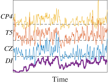
We tried to predict the drowsiness index for each subject every 10 seconds, which is called a sample point in this paper. All 30 EEG channels were used in feature extraction. We epoched 30-second EEG signals right before each sample point, and computed the average power spectral density (PSD) in the theta band (4-7.5 Hz) for each channel using Welch’s method [39], as research [25] has shown that theta band spectrum is a strong indicator of drowsiness. The theta band powers for three selected channels and the corresponding drowsiness index for a typical subject are shown in Fig. 1. The correlation coefficients between the drowsiness index and CZ, T5 and CP5 theta band powers are 0.3005, 0.2706, and 0.3129, respectively, indicating considerable correlation.
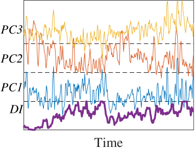
Next, we converted the 30 theta band powers to dBs. To remove noises or bad channel readings, we removed channels whose maximum dBs were larger than 20. We then normalized the dBs of each remaining channel to mean zero and standard deviation one, and extracted a few (usually around 10) leading principal components, which accounted for 95% of the variance. The projections of the dBs onto these principal components were then normalized to and used as our features. Three such features for the same subject in Fig. 1 are shown in Fig. 1. The correlation coefficients between the drowsiness index and the first three principal component scores are 0.2094, -0.6518 and 0.0169, respectively. Note that the maximum correlation is significantly improved by using the principal component features.
III-C Algorithms
We compare the performances of five different sample selection strategies:
-
1.
Baseline (BL), which randomly selects unlabeled samples for labelling.
- 2.
-
3.
Enhanced QBC (EQBC), which is the QBC above enhanced by the EBMAL.
- 4.
-
5.
Enhanced EMCM (EEMCM), which is the EMCM above enhanced by the EBMAL.
All five approaches build a linear ridge regression model from the labeled samples, as in [41]. The ridge parameter was used in all five algorithms.
III-D Evaluation Process and Performance Measures
From the experiments we already knew the drowsiness indices for all 360 samples, obtained every 10 seconds from the first 3,600 seconds data. To evaluate the performances of different algorithms, for each subject, we first randomly selected 80% of the 360 samples as our pool111For a fixed pool, EQBC and EEMCM give a deterministic selection sequence because there is no randomness involved. So, we need to vary the pool in order to study the statistical properties of EQBC and EEMCM. We did not use the traditional bootstrap approach, i.e., sampling with replacement to obtain the same number of samples as the original pool, because bootstrap introduces duplicate samples in the new pool, which does not happen in practice (a subject cannot have completely identical EEG responses at two different time instants), and also worsens the performances of QBC and EMCM (they may select multiple identical samples to label in the same batch)., and then identified five samples to label in each batch by different algorithms, built a ridge regression model, and computed the root mean squared error (RMSE) and correlation coefficient (CC) as performance measures. The maximum number of samples to be labeled was fixed to be 60, corresponding to 12 batches.
We ran this evaluation process 30 times, each time with a randomly chosen 80% population pool, to obtain statistically meaningful results.
III-E Experimental Results
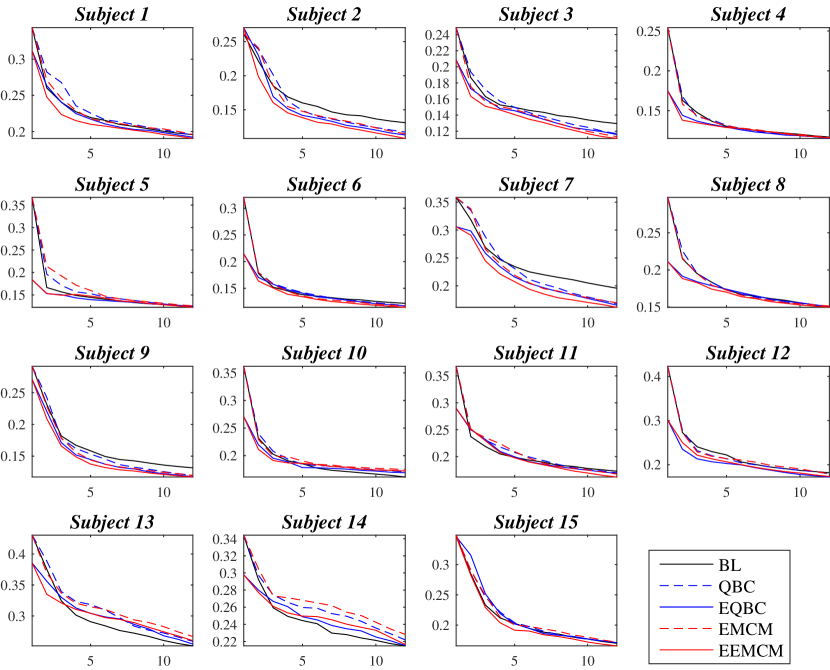
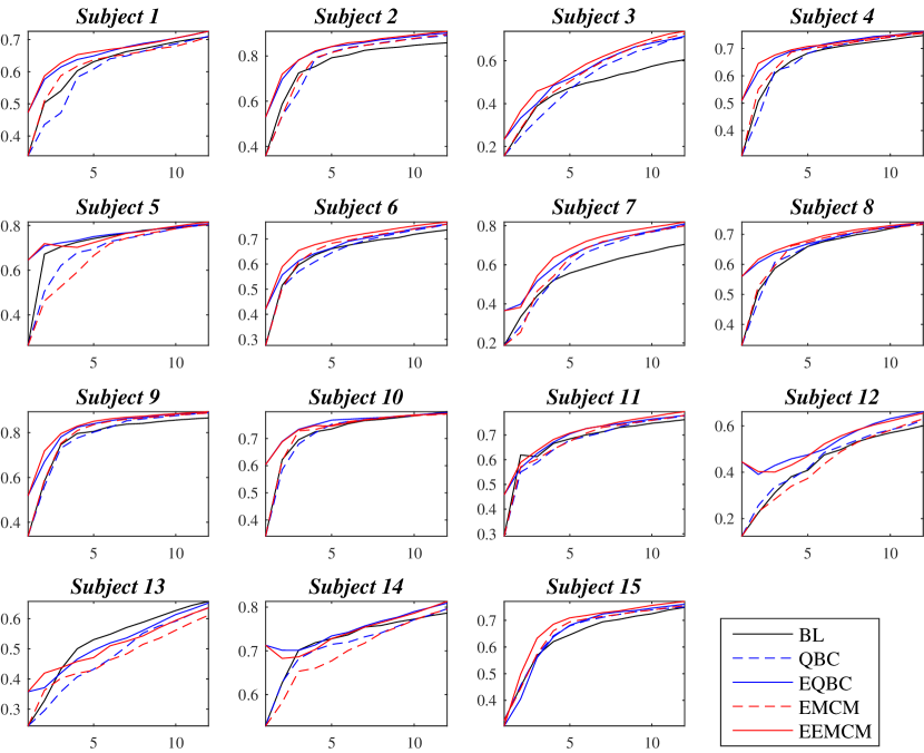
The average RMSEs and CCs for the five algorithms across the 15 subjects are shown in Fig. 2, and the RMSEs and CCs for the individual subjects are shown in Fig. 3. Observe that all methods give better RMSEs and CCs as increases, which is intuitive. QBC and EMCM had very similar performance: both were comparable to or slightly worse than BL for small , but as increased, they started to outperform BL. Remarkably, with the help of EBMAL, both EQBC and EEMCM outperformed the other three approaches for all , although the performance improvement of EQBC and EEMCM over QBC and EMCM diminished as increased.
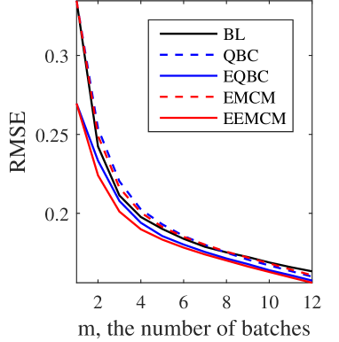
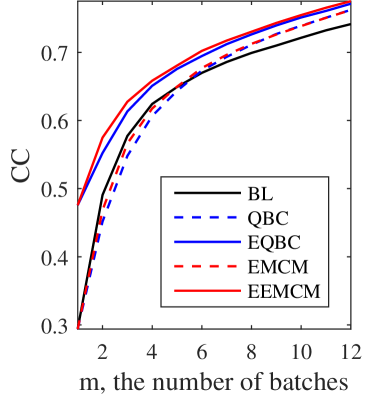
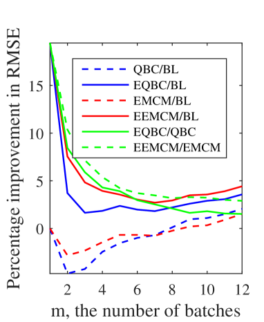
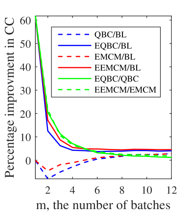
To better visualize the performance differences among different algorithms, in Fig. 4 we plot the percentage performance improvement between different pairs of algorithms. Observe that although QBC and EMCM did not outperform BL for small , the corresponding EQBC and EEMCM achieved the largest performance improvements over BL (and also QBC and EMCM) for small , especially when . This indicates that the new initialization strategy in EBMAL is indeed effective.
We also performed non-parametric multiple comparison tests using Dunn’s procedure [15, 16] to determine if the differences between different pair of algorithms were statistically significant, with a -value correction using the False Discovery Rate method [4]. The -values for RMSEs and CCs for different are shown in Tables I and II, respectively, where the statistically significant ones are marked in bold. Observe that QBC and EMCM had statistically significantly better RMSEs and CCs than BL for large , but EQBC and EEMCM had statistically significantly better RMSEs and CCs for almost all . The performance improvement of EQBC over QBC, and EEMCM over EMCM, was statistically significant for small .
| QBC | EQBC | EMCM | EEMCM | EQBC | EEMCM | |
|---|---|---|---|---|---|---|
| vs | vs | vs | vs | vs | vs | |
| BL | BL | BL | BL | QBC | EMCM | |
| 1 | .5000 | .0000 | .5000 | .0000 | .0000 | .0000 |
| 2 | .1330 | .0078 | .4294 | .0032 | .0002 | .0043 |
| 3 | .1895 | .0648 | .4896 | .0200 | .0100 | .0249 |
| 4 | .4157 | .0763 | .3026 | .0094 | .0589 | .0366 |
| 5 | .3761 | .0652 | .2203 | .0067 | .1040 | .0381 |
| 6 | .2022 | .0296 | .1483 | .0013 | .1434 | .0260 |
| 7 | .1464 | .0236 | .1013 | .0004 | .1474 | .0267 |
| 8 | .1371 | .0180 | .0668 | .0003 | .1217 | .0388 |
| 9 | .0565 | .0128 | .0354 | .0001 | .2063 | .0410 |
| 10 | .0213 | .0047 | .0155 | .0000 | .2828 | .0490 |
| 11 | .0052 | .0018 | .0064 | .0000 | .3371 | .0533 |
| 12 | .0022 | .0008 | .0018 | .0000 | .3970 | .0852 |
| QBC | EQBC | EMCM | EEMCM | EQBC | EEMCM | |
|---|---|---|---|---|---|---|
| vs | vs | vs | vs | vs | vs | |
| BL | BL | BL | BL | QBC | EMCM | |
| 1 | .5000 | .0000 | .5000 | .0000 | .0000 | .0000 |
| 2 | .0814 | .0003 | .3963 | .0032 | .0000 | .0000 |
| 3 | .4090 | .0041 | .3842 | .0059 | .0038 | .0170 |
| 4 | .3035 | .0020 | .1289 | .0004 | .0079 | .0096 |
| 5 | .1515 | .0022 | .0436 | .0002 | .0310 | .0366 |
| 6 | .0661 | .0003 | .0175 | .0000 | .0278 | .0200 |
| 7 | .0103 | .0001 | .0038 | .0000 | .0762 | .0114 |
| 8 | .0061 | .0000 | .0018 | .0000 | .0965 | .0197 |
| 9 | .0013 | .0000 | .0003 | .0000 | .1687 | .0251 |
| 10 | .0001 | .0000 | .0001 | .0000 | .2663 | .0290 |
| 11 | .0000 | .0000 | .0000 | .0000 | .3231 | .0255 |
| 12 | .0000 | .0000 | .0000 | .0000 | .3511 | .0407 |
It is also interesting to study if each of the three enhancements proposed in Section II-D are necessary, and if so, what their individual effect is. For this purpose, we constructed three modified versions of the EBMAL algorithms: EBAML1, which employs only the first enhancement on more representative initialization; EBAML2, which employs only the second enhancement on better outlier handling; and, EBMAL3, which employs only the third enhancement on diversity. We then applied them to EMCM (the resulting algorithms are called EEMCM1, EEMCM2, and EEMCM3, respectively) and compared their performances with the baseline EMCM and the complement EEMCM. The results, averaged over 30 runs and 15 subjects, are shown in Fig. 5. Observe that every enhancement outperformed the baseline EMCM. More specifically, the first enhancement on more representative initialization helped when was very small, especially at zero; the second and third enhancements on outlier handling and diversity helped when became larger. By combining the three enhancements, EEMCM achieved the best performance at both small and large . This suggests that the three enhancements are complementary, and they are all essential to the improved performance of EBMAL.
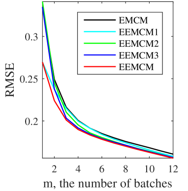
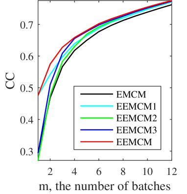
In summary, we can conclude that our proposed EBMAL approach can significantly enhance a baseline AL for regression approach, especially when the number of labeled samples is very small (including zero). The three enhancements in EBMAL all contribute to its superior performance.
IV Conclusions
Reducing the calibration data requirement in BCI systems is very important for their real-world applications. In our previous research we have extensively studied this in both online and offline BCI classification problems [42, 44, 28, 21, 46, 45], and also online regression problems [41]. This paper has proposed a novel EBMAL approach for offline BCI regression problems, and used EEG-based driver drowsiness estimation as an example to validate its performance. EBMAL solves the following problems: given a pool of unlabeled samples, how do we optimally select a small number of them to label so that an accurate regression model can be built from them to label the rest? Our proposed approach improves upon a baseline AL algorithm by increasing the reliability, representativeness and diversity of the selected samples to achieve better regression performance. To our best knowledge, this is the first time that active learning is used for regression problems in BCI. However, EBMAL is general and it can also be applied to many other offline regression problems beyond BCI, e.g., estimating the continuous values of arousal, valence and dominance from speech signals [48] in affective computing.
References
- [1] N. Abe and H. Mamitsuka, “Query learning strategies using boosting and bagging,” in Proc. 15th Int’l Conf. on Machine Learning (ICML), Madison, WI, July 1998, pp. 1–9.
- [2] M. Alamgir, M. Grosse-Wentrup, and Y. Altun, “Multitask learning for brain-computer interfaces,” in Proc. 13th Int’l Conf. on Artificial Intelligence and Statistics (AISTATS), Sardinia, Italy, May 2010, pp. 17–24.
- [3] A. Barachant, S. Bonnet, M. Congedo, and C. Jutten, “Multiclass brain-computer interface classification by Riemannian geometry,” IEEE Trans. on Biomedical Engineering, vol. 59, no. 4, pp. 920–928, 2012.
- [4] Y. Benjamini and Y. Hochberg, “Controlling the false discovery rate: A practical and powerful approach to multiple testing,” Journal of the Royal Statistical Society, Series B (Methodological), vol. 57, pp. 289–300, 1995.
- [5] R. Burbidge, J. J. Rowland, and R. D. King, “Active learning for regression based on query by committee,” Lecture Notes in Computer Science, vol. 4881, pp. 209–218, 2007.
- [6] W. Cai, Y. Zhang, and J. Zhou, “Maximizing expected model change for active learning in regression,” in Proc. IEEE 13th Int’l. Conf. on Data Mining, Dallas, TX, December 2013.
- [7] W. Cai, Y. Zhang, S. Zhou, W. Wang, C. Ding, and X. Gu, “Active learning for support vector machines with maximum model change,” Lecture Notes in Computer Science, vol. 8724, pp. 211–216, 2014.
- [8] M. Chen, X. Tan, J. Q. Gan, L. Zhang, and W. Jian, “A batch-mode active learning method based on the nearest average-class distance (NACD) for multiclass brain-computer interfaces,” Journal of Fiber Bioengineering and Informatics, vol. 7, no. 4, pp. 627–636, 2014.
- [9] C.-H. Chuang, L.-W. Ko, T.-P. Jung, and C.-T. Lin, “Kinesthesia in a sustained-attention driving task,” Neuroimage, vol. 91, pp. 187–202, 2014.
- [10] S.-W. Chuang, L.-W. Ko, Y.-P. Lin, R.-S. Huang, T.-P. Jung, and C.-T. Lin, “Co-modulatory spectral changes in independent brain processes are correlated with task performance,” Neuroimage, vol. 62, pp. 1469–1477, 2012.
- [11] D. Cohn, Z. Ghahramani, and M. Jordan, “Active learning with statistical models,” Journal of Artificial Intelligence Research, vol. 4, pp. 129–145, 1996.
- [12] A. Delorme and S. Makeig, “EEGLAB: an open source toolbox for analysis of single-trial EEG dynamics including independent component analysis,” Journal of Neuroscience Methods, vol. 134, pp. 9–21, 2004.
- [13] B. Demir and L. Bruzzone, “A multiple criteria active learning method for support vector regression,” Pattern Recognition, vol. 47, pp. 2558–2567, 2014.
- [14] P. Donmez and J. Carbonell, “Optimizing estimated loss reduction for active sampling in rank learning,” in Proc. 25th Int’l Conf. on Machine Learning (ICML), Helsinki, Finland, July 2008, pp. 248–255.
- [15] O. Dunn, “Multiple comparisons among means,” Journal of the American Statistical Association, vol. 56, pp. 62–64, 1961.
- [16] O. Dunn, “Multiple comparisons using rank sums,” Technometrics, vol. 6, pp. 214–252, 1964.
- [17] Y. Freund, H. Seung, E. Shamir, and N. Tishby, “Selective sampling using the query by committee algorithm,” Machine Learning, vol. 28, no. 2-3, pp. 133–168, 1997.
- [18] M. Hajinoroozi, T. Jung, C. Lin, and Y. Huang, “Feature extraction with deep belief networks for driver’s cognitive states prediction from EEG data,” in Proc. IEEE China Summit and Int’l. Conf. on Signal and Information Processing, Chengdu, China, July 2015.
- [19] A. Krogh and J. Vedelsby, “Neural network ensembles, cross validation, and active learning,” in Proc. Neural Information Processing Systems (NIPS), Denver, CO, November 1995, pp. 231–238.
- [20] B. J. Lance, S. E. Kerick, A. J. Ries, K. S. Oie, and K. McDowell, “Brain-computer interface technologies in the coming decades,” Proc. of the IEEE, vol. 100, no. 3, pp. 1585–1599, 2012.
- [21] V. J. Lawhern, D. J. Slayback, D. Wu, and B. J. Lance, “Efficient labeling of EEG signal artifacts using active learning,” in Proc. IEEE Int’l Conf. on Systems, Man and Cybernetics, Hong Kong, October 2015.
- [22] C.-T. Lin, L.-W. Ko, and T.-K. Shen, “Computational intelligent brain computer interaction and its applications on driving cognition,” IEEE Computational Intelligence Magazine, vol. 4, no. 4, pp. 32–46, 2009.
- [23] C.-T. Lin, L.-W. Ko, I.-F. Chung, T.-Y. Huang, Y.-C. Chen, T.-P. Jung, and S.-F. Liang, “Adaptive EEG-based alertness estimation system by using ICA-based fuzzy neural networks,” IEEE Trans. on Circuits and Systems I, vol. 53, no. 11, pp. 2469–2476, 2006.
- [24] S. Makeig and M. Inlow, “Lapses in alertness: Coherence of fluctuations in performance and EEG spectrum,” Electroencephalography and Clinical Neurophysiology, vol. 86, pp. 23–35, 1993.
- [25] S. Makeig and T. P. Jung, “Tonic, phasic and transient EEG correlates of auditory awareness in drowsiness,” Cognitive Brain Research, vol. 4, pp. 12–25, 1996.
- [26] S. Makeig, C. Kothe, T. Mullen, N. Bigdely-Shamlo, Z. Zhang, and K. Kreutz-Delgado, “Evolving signal processing for brain-computer interfaces,” Proc. of the IEEE, vol. 100, no. Special Centennial Issue, pp. 1567–1584, 2012.
- [27] Z. Mao, V. Lawhern, L. M. Merino, K. Ball, L. Deng, J. B. Lance, K. Robbins, and Y. Huang, “Classification of non-time-locked rapid serial visual presentation events for brain-computer interaction using deep learning,” in Proc. IEEE China Summit and Int’l Conf. on Signal and Information Processing, Xi’an, China, July 2014.
- [28] A. Marathe, V. Lawhern, D. Wu, D. Slayback, and B. Lance, “Improved neural signal classification in a rapid serial visual presentation task using active learning,” IEEE Trans. on Neural Systems and Rehabilitation Engineering, vol. 24, no. 3, pp. 333–343, 2016.
- [29] M. Moghadamfalahi, J. Sourati, M. Akcakaya, H. Nezamfar, M. Haghighi, and D. Erdogmus, “Active learning for efficient querying from a human oracle with noisy response in a language-model assisted brain computer interface,” in Proc. 25th IEEE Int’l Conf. on Machine Learning for Signal Processing (MLSP), Boston, MA, September 2015, pp. 1–6.
- [30] C. Muhl, B. Allison, A. Nijholt, and G. Chanel, “A survey of affective brain computer interfaces: principles, state-of-the-art, and challenges,” Brain-Computer Interfaces, vol. 1, no. 2, pp. 66–84, 2014.
- [31] T. RayChaudhuri and L. Hamey, “Minimisation of data collection by active learning,” in Proc. IEEE Int’l. Conf. on Neural Networks, vol. 3, Perth, Australia, November 1995, pp. 1338–1341.
- [32] B. Settles and M. Craven, “An analysis of active learning strategies for sequence labeling tasks,” in Proc. Conf. on Empirical Methods in Natural Language Processing (EMNLP), Honolulu, HI, October 2008, pp. 1069–1078.
- [33] B. Settles, M. Craven, and S. Ray, “Multiple-instance active learning,” in Proc. Advances in Neural Information Processing Systems (NIPS), Vancouver, BC, Canada, December 2008, pp. 1289–1296.
- [34] B. Settles, “Active learning literature survey,” University of Wisconsin–Madison, Computer Sciences Technical Report 1648, 2009.
- [35] H. Seung, M. Opper, and H. Sompolinsky, “Query by committee,” in Proc. ACM Workshop on Computational Learning Theory, Pittsburgh, PA, July 1992, pp. 287–294.
- [36] (2011) Traffic safety facts crash stats: drowsy driving. US Department of Transportation, National Highway Traffic Safety Administration. Washington, DC. [Online]. Available: http://www-nrd.nhtsa.dot.gov/pubs/811449.pdf
- [37] J. van Erp, F. Lotte, and M. Tangermann, “Brain-computer interfaces: Beyond medical applications,” Computer, vol. 45, no. 4, pp. 26–34, 2012.
- [38] C.-S. Wei, Y.-P. Lin, Y.-T. Wang, T.-P. Jung, N. Bigdely-Shamlo, and C.-T. Lin, “Selective transfer learning for EEG-based drowsiness detection,” in Proc. IEEE Int’l Conf. on Systems, Man and Cybernetics, Hong Kong, October 2015, pp. 3229–3232.
- [39] P. Welch, “The use of fast Fourier transform for the estimation of power spectra: A method based on time averaging over short, modified periodograms,” IEEE Trans. on Audio Electroacoustics, vol. 15, pp. 70–73, 1967.
- [40] J. Wolpaw and E. W. Wolpaw, Eds., Brain-Computer Interfaces: Principles and Practice. Oxford, UK: Oxford University Press, 2012.
- [41] D. Wu, C.-H. Chuang, and C.-T. Lin, “Online driver’s drowsiness estimation using domain adaptation with model fusion,” in Proc. Int’l Conf. on Affective Computing and Intelligent Interaction, Xi’an, China, September 2015, pp. 904–910.
- [42] D. Wu, B. J. Lance, and V. J. Lawhern, “Active transfer learning for reducing calibration data in single-trial classification of visually-evoked potentials,” in Proc. IEEE Int’l Conf. on Systems, Man, and Cybernetics, San Diego, CA, October 2014.
- [43] D. Wu, B. J. Lance, and T. D. Parsons, “Collaborative filtering for brain-computer interaction using transfer learning and active class selection,” PLoS ONE, 2013.
- [44] D. Wu, V. J. Lawhern, W. D. Hairston, and B. J. Lance, “Switching EEG headsets made easy: Reducing offline calibration effort using active weighted adaptation regularization,” IEEE Trans. on Neural Systems and Rehabilitation Engineering, vol. 24, no. 11, pp. 1125–1137, 2016.
- [45] D. Wu, V. J. Lawhern, and B. J. Lance, “Reducing BCI calibration effort in RSVP tasks using online weighted adaptation regularization with source domain selection,” in Proc. Int’l Conf. on Affective Computing and Intelligent Interaction, Xi’an, China, September 2015.
- [46] D. Wu, V. J. Lawhern, and B. J. Lance, “Reducing offline BCI calibration effort using weighted adaptation regularization with source domain selection,” in Proc. IEEE Int’l Conf. on Systems, Man and Cybernetics, Hong Kong, October 2015.
- [47] D. Wu and T. D. Parsons, “Active class selection for arousal classification,” in Proc. 4th Int’l Conf. on Affective Computing and Intelligent Interaction, vol. 2, Memphis, TN, October 2011, pp. 132–141.
- [48] D. Wu, T. D. Parsons, E. Mower, and S. S. Narayanan, “Speech emotion estimation in 3D space,” in Proc. IEEE Int’l Conf. on Multimedia & Expo (ICME), Singapore, July 2010, pp. 737–742.
- [49] Y. Zhao and Q. Ji, “A new active learning method for EEG multi-class classification,” Energy Procedia, vol. 13, pp. 3263–3268, 2011.