Efficient and flexible MATLAB implementation of 2D and 3D elastoplastic problems
Abstract
We propose an effective and flexible way to implement 2D and 3D elastoplastic problems in MATLAB using fully vectorized codes. Our technique is applied to a broad class of the problems including perfect plasticity or plasticity with hardening and several yield criteria. The problems are formulated in terms of displacements, discretized by the implicit Euler method in time and the finite element method in space, and solved by the semismooth Newton method. We discuss in detail selected models with the von Mises and Prager-Drucker yield criteria and four types of finite elements. The related codes are available for download. A particular interest is devoted to the assembling of tangential stiffness matrices. Since these matrices are repeatedly constructed in each Newton iteration and in each time step, we propose another vectorized assembling than current ones known for the elastic stiffness matrices. The main idea is based on a construction of two large and sparse matrices representing the strain-displacement and tangent operators, respectively, where the former matrix remains fixed and the latter one is updated only at some integration points. Comparisons with other available MATLAB codes show that our technique is also efficient for purely elastic problems. In elastoplasticity, the assembly times are linearly proportional to the number of integration points in a plastic phase and additional times due to plasticity never exceed assembly time of the elastic stiffness matrix.
keywords:
MATLAB code vectorization , Elastoplasticity , Finite element method , Tangential stiffness matrix , Semismooth Newton method1 Introduction
The paper is focused on implementation of time-discretized elastoplastic problems formulated in terms of displacements. These problems include the following nonlinear variational equation [7, 15] defined in each time step :
where , , is a bounded domain with the Lipschitz boundary . The parts and are open and disjoint. On , the Dirichlet boundary conditions are prescribed and represented by a given displacement function . The testing functions belong to the space of -functions vanishing on . Further,
are the prescribed volume and surface forces acting in and on , respectively. At any point
denote the infinitesimal strain tensor and the stress tensor and is a nonlinear stress-strain operator. The operator also depends on the plastic strain and other internal variables known from the previous time step . This operator varies depending on a particular constitutive model and is defined in an implicit form, in general. Although is nonsmooth, its semismoothness was proven for some elastoplastic models, see, e.g., [8, 14, 18, 21].
We follow a current computational procedure consisting of the following steps [7, 15, 20, 21]:
-
space discretization of by the finite element method (FEM);
-
solution of a resulting discretized system by the (semismooth) Newton method;
Due to the possible presence of limit loads [7, 11, 10] leading to locking phenomena, implementations in elastoplasticity utilize higher order finite elements. Their assemblies require suitable quadrature rules of higher order [2, 7]. To use the semismooth Newton method, one must find a generalized derivative of w.r.t. the strain variable, the so-called consistent tangent operator
After the solution is found, one can easily update , and the internal variables at the level of integration points, and continue with the next time step.
For a computer implementation, it is crucial to find a suitable assembly of the so-called tangential stiffness matrix based on the operator . We propose and explain in detail an efficient implementation of the tangential stiffness matrix in the form
| (1) |
where is a sparse matrix representing the strain-displacement operator at all integration points. The matrix is a block diagonal matrix and each block contains the operator for a particular integration point. The matrix is also block diagonal and represents its elastic counterpart. It is applied to assembly the elastic stifness matrix in the form
| (2) |
The matrices can be precomputed and only the matrix needs to be partially reassembled in each Newton iteration. Although some MATLAB elastoplasticity codes are already available [5, 19, 22] and applied to various elastoplasticity models [4, 20, 21], they are not at all or only partially vectorized. The vectorization replaces time consuming loops by operations with long vectors and arrays and proves to be reasonably scalable and fast for large size problems. It typically takes only few minutes to solve studies elastoplastic benchmarks with several milion on unknows on current computers. Authors are not aware of any other fully vectorized Matlab assembly of elastoplastic problems.
Our code is available for download [6] and provides several computing benchmarks including
-
elastic and elastoplastic models with von Mises or Drucker-Prager yield criteria;
-
finite element implementations of P1, P2, Q1, Q2 elements in both 2D and 3D.
Crucial functions are written uniformly regardless on these options. For the sake of brevity, we shall describe only 3D problems in this paper. Its plane strain reduction to 2D is usually straightforward and introduced within the code. Therefore, we set from now on. Although the paper is focused on an assembly of the tangential stiffness matrix, it is worth mentioning that the code contains complex implementation of elastic and elastoplastic problems defined on fixed geometries. In particular, there are included fully vectorized procedures for specific mesh generation, volume and surface forces. The solver is based on the semismooth Newton method combined with time stepping which can be adaptive, if necessary.
The rest of the paper is organized as follows. In Section 2, we introduce a simplified scheme of elastoplastic constitutive problems and define the stress-strain operator . Then we introduce examples of the operators and for some constitutive models. In Section 3, the finite element discretization of problem is described. In Section 4, an algebraic formulation of the elastoplastic problem and the semismooth Newton method are introduced. In Section 5, basic MATLAB notation is introduced. In Sections 6 and 7, we describe assembly of the elastic and tangent stiffness matrices and the vector of internal forces. In Section 8, we illustrate the efficiency of the vectorized codes on particular 2D and 3D examples. The paper also contains Appendix, where reference elements, local basic functions and suitable quadrature formulas are summarized for the used finite elements.
2 Elastoplastic constitutive model
In this section, we introduce an elastoplastic constitutive model and its implicit Euler discretization with respect to a time variable The constitutive model is an essential part of the overall elastoplastic problem. It is defined at any point . We shall assume that the model: satisfies the principle of maximum plastic dissipation; is based on linear elasticity; and contains optionally internal variables like kinematic or isotropic hardening. These assumptions enable to introduce variational formulation of the overall elastoplastic problem important for solvability analysis [9]. More general constitutive models can be found, e.g., in [7, 15]. The initial value constitutive problem has the following scheme [5, 9, 18]:
Given the history of the infinitesimal strain tensor , , and the initial values ; find the stress tensor , the plastic strain , internal variables and thermodynamical forces such that
| (3) |
hold for each instant , where is a finite dimensional space with the scalar product , is a Lipschitz continuous and strongly monotone function, is a closed convex set with a nonempty interior, and is the fourth order elastic tensor.
The elastic part of the strain tensor is denoted as
and the doubles , are called the generalized stress and strain, respectively. Notice that belongs to the normal cone of at . The definition of depends on the used internal variables. For example, one can set , , and for kinematic hardening, isotropic hardening, and perfect plasticity (no internal variables), respectively. Further, we shall assume that is represented by two material parameters (isotropic material), e.g., by the bulk modulus and the shear modulus in the form
| (4) |
Here, denotes the tensor product of unit (second order) tensors and , where for any . Consequently, the Hooke’s law states the linear relation between the stress and the elastic strain tensors
| (5) |
The set is often in the form
where is a convex yield function. This fact allows to rewrite (3) by the Karush-Kuhn-Tucker (KKT) conditions:
| (6) |
Here, stands for the plastic multiplier and is a subdifferential operator. The formulation (6) is broadly used in engineering practice [7, 15] and it is convenient for finding analytical or semianalytical solution of the constitutive problem [20, 21].
2.1 The implicit discretization of the constitutive problem
Let us consider a partition of the time interval in the form
and denote , , , , . The -th step of the incremental constitutive problem discretized by the implicit Euler method reads as:
Given , and , find , , , , and satisfying:
| (7) |
Under the assumptions mentioned above, problem (7) has a unique solution [18]. Therefore, one can define the stress-strain operator as follows:
In general, the function is implicit. Nevertheless, it is well-known that problem (7) can be simplified and, sometimes, its solution can be found in a closed form. To this end the elastic predictor – plastic corrector method is applied. Within the elastic prediction, it is checked whether the trial generalized stress , is admissible or not. If then
is the solution to (7) representing the elastic response. Otherwise, (7)3 reduces into and , and the plastic correction (return mapping) of the trial generalized stress is necessary. From [18], it follows that is Lipschitz continuous in . Therefore, one can define a function
representing a generalized Clark derivative of . Clearly, if is differentiable at then . One can also investigate the semismoothness of under the assumption that is semismooth in [18].
In the elastic case, no plastic strain and internal variables occur, , the stress-strain operator and its derivative simplify as
| (8) |
Further, we introduce two particular examples of elastoplastic models and their operators and , for illustration.


2.2 Von Mises yield criterion and linear kinematic hardening
This model corresponds to the choice
where is the deviatoric part of . If then the set of admissible stress tensors is a cylinder aligned with the hydrostatic axis, see Figure 1. The kinematic hardening causes translation of the cylinder in the normal direction to the yield surface. The corresponding solution of (7) can be found, e.g., in [3, 5]. We arrive at:
| (9) |
| (10) |
where
Further, the hardening variable and the plastic strain are updated as follows:
| (11) |
Notice that if we arrive at formulas for the perfect plastic model with the von Mises yield criterion.
2.3 Drucker-Prager yield criterion and perfect plasticity
In perfect plasticity, the internal variables and are not included in the model and . The Drucker-Prager yield function is defined as follows:
where are given material parameters. The corresponding set of admissible stress tensors is depicted in Figure 1. It is a cone aligned with the hydrostatic axis. The operators and can be found in closed forms [7, 20] by solving the system (7). To summarize their forms, we distinguish three different cases and define the following auxiliary notation:
-
1.
Elastic response occurs if . Then , and .
-
2.
Return to the smooth portion of the yield surface occurs if and . Then,
-
3.
Return to the apex of the yield surface occurs if . Then,
where is a zero fourth order tensor, i.e., for any .
3 Finite element discretization
The standard Galerkin method leads to the following discrete counterpart of problem :
where is a finite dimensional approximation of and , , , and are suitable approximations of , , , and , respectively. Beside these approximations, one must also take into account a numerical integration specified below. The finite element method corresponds to a specific choice of . In particular, we shall consider conforming and isoparametric finite elements of Lagrange type in 3D and define the corresponding basis functions of . For more detail, we refer to [2].
Let denote a reference element w.r.t. to Cartesian coordinates . The reference element is usually a convex polyhedron (in our case, either a tetrahedron or a hexahedron) and its boundary consists of sides . On , we prescribe: a space of dimension , basis functions of , and nodes , such that , . Further, the domain is covered by a regular triangulation , i.e., . We assume that any element can be described by nodes , , and by the following nondegenerative transformation of :
| (12) |
Then the so-called iso-parametric transformation (12) maps onto for and any side has a corresponding side . It is required that: any side is either an intersection of two neighboring elements or a part of the boundary ; if , , then is also a nodal point of . Further, we standardly assume that if some node belongs to then also in order to reflect the curvature of the original domain .
Making use of the transformation (12), one can define the local basis function , for any element :
| (13) |
Define the set of all nodes corresponding to the triangulation , i.e., for any and . Let denote a number of nodes from . For any node , , we define the function as follows:
| (14) |
The assumption on conforming finite elements means that the space and the reference nodes , , are such that the functions , , are continuous. This holds, e.g., for simplicial P1, P2, or quadrilateral Q1, Q2, elements, , see [2]. Let denote the space generated by (global) basis functions , , i.e., . It is a space of continuous and piecewise smooth functions of the form
| (15) |
The space is a finite dimensional subspace of and analogously, . The required space is the subspace of which does not contain basis functions corresponding to the nodes lying on , i.e.,
where . We shall also use the notation .
In order to evaluate volume integrals, we standardly split the domain into elements and use the transformation (12) of onto . We have the following transforming formulas [2]:
| (22) | |||
| (23) |
where denotes a Jacobian matrix (referred to as Jacobian) on . Finally, we consider a numerical quadrature in and write it in an abstract form:
| (24) |
where are the quadrature points and are the corresponding weights for . For example, we shall use the following formulas:
| (25) |
| (26) |
where the nodes correspond to within the transformation (12) and
| (27) |
From these formulas, one can easily derive the required volume integrals through important for assembly of the stiffness matrix and of the vectors of volume forces (internal and external), see Sections 6 and 7. Examples of finite elements and convenient numerical quadratures are introduced in the Appendix.
4 Algebraic problem and Newton-like method
An algebraic form of problem reads as:
Here, , and are the algebraic counterparts of , and , respectively. For example,
The remaining notation is defined as follows:
Problem can be simply transformed to a system of nonlinear equations by elimination of rows that correspond to the Dirichlet boundary conditions:
where and arise from and , respectively, by the elimination.
In order to introduce the semismooth Newton method, we define a generalized gradient of at :
The corresponding algorithm reads as:
Algorithm 1 (ALG-NEWTON).
where , and for any . In each -th Newton iteration, we solve the linear problem with the tangent stiffness matrix . This problem can be transformed to the linear system of equations
| (28) |
by the elimination of the Dirichlet nodes. Assembly of and for some is derived in detail in Sections 6 and 7 where the indices and will be omitted, for the sake of simplicity.
It is well known that convergence of the Newton method is superlinear under the assumption that is close to the solution of . Alternatively, one can apply a damped version of the Newton method in elastoplasticity, see, e.g., [17].
5 Basic MATLAB notation
To distinguish notation for MATLAB commands and expressions in the next sections, a typescript is used (e.g., ELEM, COORD, etc.). Instead of subscripts, we use the underscore symbol in MATLAB, e.g., n_n, n_e, n_q, etc. Further, to be the codes vectorized (without long for-cycles), we work with arrays and use standard MATLAB commands like
repmat, kron, reshape, .*, ./, sum.
Let and be numbers of nodes from and elements from , respectively, and recall that and denote number of nodes and quadrature points within a finite element, respectively. Further, we define , i.e., a number of all integration points , , .
We use a array U for storage of nodal displacements. In order to receive the corresponding displacement vector , it suffices to use the command U(:), i.e., U(:). Further, it is convenient to define the logical array Q which indicates the nodes belonging to , i.e., the nodes where the Dirichlet boundary condition is not prescribed. Then the restricted displacement vector satisfies U(Q). Similarly, one can restrict the stiffness matrix and the vectors of external and internal forces, and . Once these objects are at disposal in MATLAB, the system (28) of linear equations can be solved by the following commands (omitting indices and ):
dU=zeros(3,n_n); dU(Q) = K(Q,Q)\(f(Q)-F(Q));
Further, stress and strain tensors, and , are represented standardly by the following vectors:
respectively111Within implementation, it is necessary to keep the different representations of stress-based and strain-based tensors..
These vectors are evaluated at each integration point , , . So, we shall consider arrays S and E for the stress and strain components, respectively. In particular, the array S will be used in for storage the values of . Similarly, a array DS will store for the corresponding values of at all integration points.
6 Assembly of elastic stiffness matrix
The construction of the elastic stiffness matrix K_elast from (2) is realized by the function
K_elast=elastic_stiffness_matrix(ELEM, COORD, shear, bulk, DHatP1, DHatP2, DHatP3, WF)
within our codes. This function has the following input data:
ELEM is an array that contains indices of nodes belonging to each element and COORD is a array containing coordinates of the nodes. We construct these standard arrays for specific geometries by vectorized procedures. Nevertheless, one can import them from a mesh generator. Further, shear and bulk denote arrays representing values of the shear () and bulk () moduli at each integration points, respectively. These values are usually computed from the Young modulus and the Poisson ratio, see Section 8. The arrays DHatP1, DHatP2, DHatP3 store the basis functions gradient values
respectively. WF denotes a array of the weight coefficients defining a numerical quadrature. The arrays WF, DHatP1, DHatP2 and DHatP3 are obtained by the following functions:
[Xi, WF] = quadrature_volume(elem_type); [HatP,DHatP1,DHatP2,DHatP3] = local_basis_volume(elem_type, Xi);
where elem_type specifies P1, P2, Q1 or Q2 finite elements. Additionally, arrays Xi, HatP contain local coordinates of and the basis functions values
respectively. A quadrature rule is predefined for any element, see the Appendix. Nevertheless, one can easily change the rules within the function quadrature_volume.
6.1 Jacobian, its determinant and inverse, derivatives of local basis functions
The Jacobian from (23) needs to be evaluated at each integration point. Its components are stored in arrays denoted as J11, J12,, J33. These components are computed using the arrays DHatP1, DHatP2, DHatP3, COORD and ELEM. By a suitable replication of DHatP1, DHatP2, DHatP3, we obtain the following arrays:
DHatPhi1=repmat(DHatP1,1,n_e); DHatPhi2=repmat(DHatP2,1,n_e); DHatPhi3=repmat(DHatP3,1,n_e);
Further, from COORD and ELEM, we derive arrays COORDint1, COORDint2, COORDint3 containing the first, second, and third coordinates (x, y and z components) of nodes that define an element containing a particular integration point:
COORDe1=reshape(COORD(1,ELEM(:)),n_p,n_e); COORDint1=kron(COORDe1,ones(1,n_q)); COORDe2=reshape(COORD(2,ELEM(:)),n_p,n_e); COORDint2=kron(COORDe2,ones(1,n_q)); COORDe3=reshape(COORD(3,ELEM(:)),n_p,n_e); COORDint3=kron(COORDe3,ones(1,n_q));
Now, one can easily compute the components of Jacobians at integration points:
J11=sum(COORDint1.*DHatPhi1); J12=sum(COORDint2.*DHatPhi1); J13=sum(COORDint3.*DHatPhi1); J21=sum(COORDint1.*DHatPhi2); J22=sum(COORDint2.*DHatPhi2); J23=sum(COORDint3.*DHatPhi2); J31=sum(COORDint1.*DHatPhi3); J32=sum(COORDint2.*DHatPhi3); J33=sum(COORDint3.*DHatPhi3);
Let DET and Jinv11, , Jinv33 be arrays representing the determinant and the components of the inverse matrix to Jacobian. These arrays can be found by the following commands:
DET = J11.*(J22.*J33-J23.*J32) - J12.*(J21.*J33-J23.*J31) + J13.*(J21.*J32-J22.*J31); Jinv11 = (J22.*J33-J23.*J32)./DET; Jinv12 = -(J12.*J33-J13.*J32)./DET; Jinv13 = (J12.*J23-J13.*J22)./DET; Jinv21 = -(J21.*J33-J23.*J31)./DET; Jinv22 = (J11.*J33-J13.*J31)./DET; Jinv23 = -(J11.*J23-J13.*J21)./DET; Jinv31 = (J21.*J32-J22.*J31)./DET; Jinv32 = -(J11.*J32-J12.*J31)./DET; Jinv33 = (J11.*J22-J12.*J21)./DET;
According to (27), we evaluate
and store these values into arrays DPhi1, DPhi2, DPhi3:
DPhi1 = repmat(Jinv11,n_p,1).*DHatPhi1 + repmat(Jinv12,n_p,1).*DHatPhi2 + repmat(Jinv13,n_p,1).*DHatPhi3; DPhi2 = repmat(Jinv21,n_p,1).*DHatPhi1 + repmat(Jinv22,n_p,1).*DHatPhi2 + repmat(Jinv23,n_p,1).*DHatPhi3; DPhi3 = repmat(Jinv31,n_p,1).*DHatPhi1 + repmat(Jinv32,n_p,1).*DHatPhi2 + repmat(Jinv33,n_p,1).*DHatPhi3;
6.2 Strain-displacement relation
To represent a relation between the strain array E and the displacement array U, we shall construct a array B. By using this array, the strain-displacement relation can be written by the following command:
E = reshape(B*U(:),6,n_int);
The array B is a large and sparse matrix, therefore its construction will be done by using the command sparse,
B = sparse(iB(:),jB(:),vB(:), 6*n_int,3*n_n);
Here, vB, iB, jB are arrays containing non-zero values of B and the corresponding -th and -th indices, respectively. The size follows from the local strain-displacement relation defined at each quadrature point. It is well-known that the strain-displacement relation at a point , and can be written as follows:
| (29) |
where , , . Each column of the array vB contains components of the matrix from (29). In particular, we arrive at
n_b=18*n_p; vB=zeros(n_b,n_int); vB(1:18:n_b-17,:)=DPhi1; vB(10:18:n_b- 8,:)=DPhi1; vB(18:18:n_b ,:)=DPhi1; vB(4:18:n_b-14,:)=DPhi2; vB( 8:18:n_b-10,:)=DPhi2; vB(17:18:n_b-1,:)=DPhi2; vB(6:18:n_b-12,:)=DPhi3; vB(11:18:n_b- 7,:)=DPhi3; vB(15:18:n_b-3,:)=DPhi3;
The arrays iB and jB of indices can be derived as follows:
AUX=reshape(1:6*n_int, 6,n_int); iB=repmat(AUX, 3*n_p,1); AUX1=[1;1;1]*(1:n_p); AUX2 = [2;1;0]*ones(1,n_p); AUX3=3*ELEM((AUX1(:))’,:)-kron(ones(1,n_e),AUX2(:)); jB=kron(AUX3,ones(6,n_q));
6.3 Elastic stiffness matrix
In elasticity, we have as follows from (8). To store these values at all integration points, we use the array DS mentioned above:
IOTA=[1;1;1;0;0;0]; VOL=IOTA*IOTA’; DEV=diag([1,1,1,1/2,1/2,1/2])-VOL/3; DS=2*DEV(:)*shear+VOL(:)*bulk;
Here, IOTA, VOL, DEV denote the MATLAB counterparts of the tensors , , and , respectively. It is important to note that the definition of DEV enables to transform a strain-type tensor to a stress-type tensor.
Further, we shall need the following array
WEIGHT = abs(DET).*repmat(WF, 1,n_e);
From the arrays DS and WEIGHT, we arrive at the following block diagonal (sparse) matrix D_elast:
AUX=reshape(1:6*n_int,6,n_int); iD=repmat(AUX,6,1); jD=kron(AUX,ones(6,1)); vD=DS.*repmat(WEIGHT,36,1); D_elast=sparse(iD,jD,vD,6*n_int,6*n_int );
The elastic stiffness matrix can be assembled similarly as in formula (26).
The assembly of the array K_elast reads as
K_elast=B’*D_elast*B;
7 Assembly of the tangent stiffness matrix and vector of internal forces
The tangent stiffness matrix K_tangent based on (1) and the vector F of internal forces are updated in each time step and in each Newton iteration within the loading process. To this end, it suffices to update only the arrays S, DS and use the arrays B, iD, jD, WEIGHT, K_elast and D_elast which are the output data from the function elastic_stiffness_matrix. This is the main advantage of the presented assembly.
The assembly of K_tangent and F read as
vD = repmat(WEIGHT,9,1).*DS ; D_tangent = sparse( iD(:),jD(:),vD(:), 6*n_int,6*n_int ) ; K_tangent = K_elast+B’*(D_tangent-D_elast)*B; F = B’*reshape(S.*repmat(WEIGHT,6,1), 6*n_int,1);
and the arrays S and DS are created by the function
constitutive_problem
described in Sections 7.1 and 7.2 von von Mises and Drucker-Prager yield criteria.
7.1 Von Mises yield criterion and kinematic hardening
According to Section 2.2, the input data to the function constitutive_problem are:
E, Ep_prev, Hard_prev, shear, bulk, a , Y.
Here, E = reshape(B*U(:),6,n_int), Ep_prev and Hard_prev are arrays representing the strain tensor at current time step , the plastic strain and the kinematic hardening from the previous time step, respectively. The remaining input arrays store the material parameters , , and at all integration points.
First, we compute the MATLAB counterparts to , , , and :
E_tr=E-Ep_prev; % size(E_tr)=(6,n_int) S_tr=2*repmat(shear,6,1).*(DEV*E_tr)+repmat(bulk,6,1).*(VOL*E_tr); % size(S_tr)=(6,n_int) SD_tr=DEV*(2*repmat(shear,6,1).*E_tr)-Hard_prev; % size(SD_tr)=(6,n_int) norm_SD=sqrt(sum(SD_tr(1:3,:).*SD_tr(1:3,:))+2*sum(SD_tr(4:6,:).*SD_tr(4:6,:))); % size(norm_SD)=(1,n_int)
In order to distinguish integration points with elastic and plastic behaviour, we define a array CRIT representing the yield criterion and the corresponding logical array IND_p which indicates integration points with plastic behaviour:
CRIT=norm_SD-Y; IND_p=CRIT>0;
The elastic prediction yields
S=S_tr; DS=2*DEV(:)*shear+VOL(:)*bulk;
We apply the plastic correction at the integration points with the plastic response according to the formulas (9) and (10):
Nhat=SD_tr(:,IND_p)./repmat(norm_SD(IND_p),6,1); denom = 2*shear(IND_p)+a(IND_p); lambda=CRIT(IND_p)./denom; S(:,IND_p)=S(:,IND_p)-repmat(2*shear(IND_p).*lambda,6,1).*N_hat;
Here, the arrays Nhat, lambda represent the function and the plastic multipliers. In order to update DS, we introduce two auxiliary arrays ID and NNhat representing the terms and in (10), respectively:
ID=DEV(:)*ones(1,length(lambda));
NNhat=repmat(N_hat,6,1).*kron(N_hat,ones(6,1));
const=((2*shear(IND_p)).^2)./denom;
DS(:,IND_p)=DS(:,IND_p)-repmat(const,36,1).*ID+...
repmat((const.*Y(IND_p))./norm_SD(IND_p),36,1).*(ID-NN_hat);
Let us complete that the function constitutive_problem also contains other output data including the updated plastic strain and the hardening according to formula (11).
7.2 Drucker-Prager yield criterion and perfect plasticity
The constitutive assembly for the Drucker-Prager yield criterion and perfect plasticity is based on formulas from Section 2.3. The input data to the function constitutive_problem are now E, E_prev, shear, bulk and arrays eta and c representing plastic material parameters. The corresponding MATLAB code is summarized below. Since its structure is similar to Section 7.1, we skip some comments to this code. We only emphasize that two decision criteria are used unlike the von Mises model. To this end, we introduce logical arrays IND_s and IND_a indicating integration points where the return to the smooth portion and to the apex of the yield surface happen, respectively.
E_tr=E-Ep_prev;
S_tr=2*repmat(shear,6,1).*(DEV*E_tr)+repmat(bulk,6,1).*(VOL*E_tr);
dev_E=DEV*E_tr; % deviatoric part of E_tr
norm_E=sqrt(max(0,sum(E_tr.*dev_E))); % norm of the deviatoric strain
rho_tr=2*shear.*norm_E; % \varrho^{tr}
p_tr=bulk.*(IOTA’*E_tr); % trial volumetric stress
denom_a= bulk.*(eta.^2);
denom_s=shear+denom_a;
CRIT1= rho_tr/sqrt(2) + eta.*p_tr - c ;
CRIT2= eta.*p_tr - denom_a.*rho_tr./(shear*sqrt(2)) - c ;
IND_s = (CRIT1>0)&(CRIT2<=0); % logical array for the return to the smooth portion
IND_a = (CRIT1>0)&(CRIT2>0); % logical array for the return to the apex
S=S_tr; DS=2*DEV(:)*shear+VOL(:)*bulk;
lambda_s=CRIT1(IND_s)./denom_s(IND_s);
n_smooth=length(lambda_s);
lambda_a=(eta(IND_a).*p_tr(IND_a)-c(IND_a))./denom_a(IND_a);
n_apex=length(lambda_a);
N_hat=dev_E(:,IND_s)./repmat(norm_E(IND_s),6,1);
M_hat=repmat(sqrt(2)*shear(IND_s),6,1).*N_hat+IOTA*(bulk(IND_s).*eta(IND_s));
S(:,IND_s)=S(:,IND_s)-repmat(lambda_s,6,1).*M_hat;
S(:,IND_a)=IOTA*(c(IND_a)./eta(IND_a));
ID=DEV(:)*ones(1,n_smooth);
NN_hat=repmat(N_hat,6,1).*kron(N_hat,ones(6,1));
MM_hat=repmat(M_hat,6,1).*kron(M_hat,ones(6,1));
DS(:,IND_s)=DS(:,IND_s)-...
repmat(2*sqrt(2)*(shear(IND_s).^2).*lambda_s./rho_tr(IND_s),36,1).*(ID-NN_hat)-...
MM_hat./repmat(denom_s(IND_s),36,1);
DS(:,IND_a)=zeros(36,n_apex);
Let us complete that the function constitutive_problem also contains other output updating the plastic strain according to formulas from Section 2.3.
8 Computational Examples
Particular examples are introduced in Sections 8.1-8.3. The performance of the codes was tested with MATLAB 8.5.0.197613 (R2015a) on a computer with 64 Intel(R) Xeon(R) CPU E5-2640 v3 processors running at 2.60GHz, number of processors 2, 256 GB RAM, and 7.5 TB harddisk memory. Calculation times are given in seconds. Our codes are available for download and testing at [6]. They contain implementation of selected 2D (plain strain) and 3D problems from elasticity and elastoplasticity on predefined domains. One can choose P1, P2, Q1 or Q2 elements (see Appendix) and different levels of mesh density. Regular meshes are considered and constructed using fully vectorized procedures.
8.1 Assembly of elastic stiffness matrices and comparison with other codes
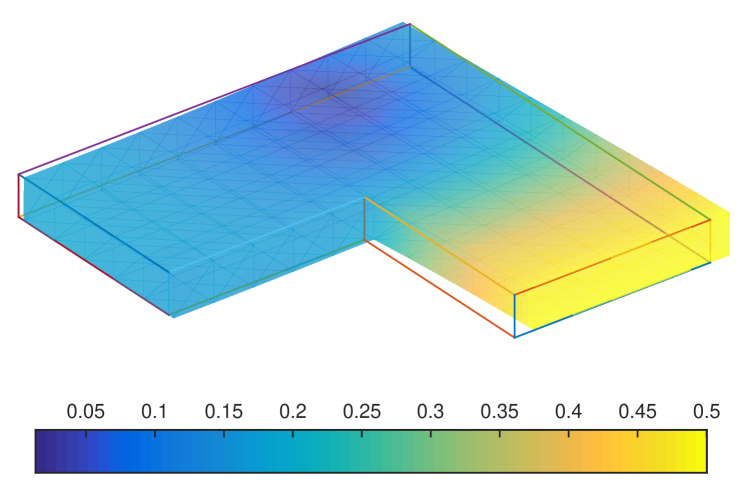
We consider a body that occupies the domain depicted in Figure 2 in plane. The corresponding 3D geometry appears by extrusion in direction. The size of the body in this direction is equal to one if the 3D problem is considered. It is assumed that prescribed forces are independent of direction to be 2D and 3D results similar. On the left and bottom sides of the depicted domain, the symmetry boundary conditions are prescribed, i.e., where is a normal vector to the boundary. On the bottom, we also prescribe nonhomogeneous Dirichlet boundary condition in the direction . Further, the constant traction of density is acting on the upper side in the normal direction and the constant volume force is prescribed in direction. The material parameters are set as follows: (Young’s modulus) and (Poisson’s ratio). The corresponding values of the bulk and shear moduli are computed standardly from and :
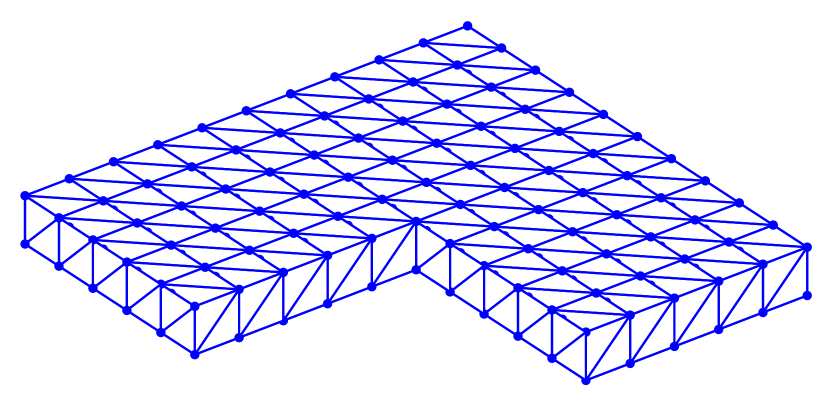
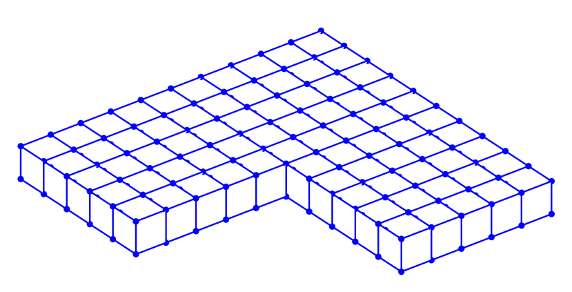
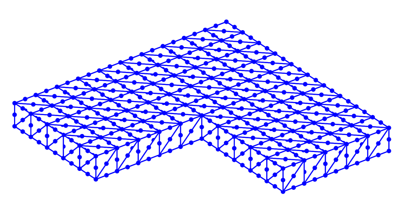
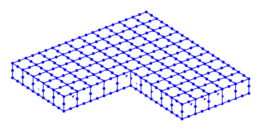
The corresponding codes are located in directory elasticity at [6]. Stiffness matrices are generated for a sequence of uniformly refined meshes in 2D and 3D. Coarse (level 0) 3D meshes are displayed in Figure 3. Results were obtained by the script
elasticity_assembly_test;
located in subdirectories elasticity_2D and elasticity_3D.
Corresponding assembly times are summarized in Tables 2, 2.
| size of | assembly of | |||||||
|---|---|---|---|---|---|---|---|---|
| level | ||||||||
| 3 | 9922 | 39,042 | 9922 | 29,442 | 0.06 | 0.62 | 0.17 | 0.56 |
| 4 | 39,042 | 154,882 | 39,042 | 116,482 | 0.21 | 2.40 | 0.58 | 1.89 |
| 5 | 154,882 | 616,962 | 154,882 | 463,362 | 0.72 | 9.13 | 1.70 | 8.04 |
| 6 | 616,962 | 2,462,722 | 616,962 | 1,848,322 | 2.75 | 34.58 | 6.70 | 32.19 |
| 7 | 2,462,722 | 9,840,642 | 2,462,722 | 7,383,042 | 10.42 | 148.68 | 27.17 | 130.65 |
| 8 | 9,840,642 | 39,342,082 | 9,840,642 | 29,511,682 | 39.87 | 608.70 | 112.40 | 545.08 |
| 9 | 39,342,082 | 157,327,362 | 39,342,082 | 118,005,762 | 169.52 | 16,524.98 | 528.65 | 8284.21 |
| size of | assembly of | |||||||
|---|---|---|---|---|---|---|---|---|
| level | ||||||||
| 1 | 3069 | 19,215 | 3069 | 10,875 | 0.14 | 1.55 | 0.19 | 1.51 |
| 2 | 19,215 | 133,947 | 19,215 | 71,787 | 0.43 | 12.25 | 1.18 | 11.54 |
| 3 | 133,947 | 995,571 | 133,947 | 516,531 | 3.70 | 102.07 | 9.78 | 95.87 |
| 4 | 995,571 | 7,666,659 | 995,571 | 3,907,299 | 29.13 | 1040.36 | 78.38 | 849.60 |
We observe (almost) optimal scalability: assembly times are linearly proportional to sizes of matrices. The solution of the elastic problem defined above is computed by the script
elasticity_fem;
located in subdirectories elasticity_2D and elasticity_3D.
Beside elastic stiffness matrix , the right-hand size vector is assembled by fully vectorized procedures. The procedures are written for more general volume and surface forces that need not be only constant. The displacement is computed from the linear system of equations
and displayed together with the deformed body, see Figure 2.
Performance comparison to the technique of Rahman and Valdman [13] for P1 elements is done by scripts
comparison_assembly_P1_2D_elasticity; comparison_assembly_P1_3D_elasticity;
| size of | assembly of | ||
|---|---|---|---|
| level | |||
| 6 | 25,090 | 0.12 | 0.22 |
| 7 | 99,330 | 0.53 | 1.01 |
| 8 | 395,266 | 2.25 | 4.31 |
| 9 | 1,576,962 | 9.54 | 16.23 |
| 10 | 6,299,650 | 43.01 | 70.02 |
| 11 | 25,182,210 | 180.15 | 308.68 |
| 12 | 100,696,066 | 975.82 | 1536.63 |
| size of | assembly of | ||
|---|---|---|---|
| level | |||
| 1 | 1029 | 0.03 | 0.05 |
| 2 | 6591 | 0.19 | 0.42 |
| 3 | 46,875 | 1.62 | 3.96 |
| 4 | 352,947 | 11.36 | 30.55 |
| 5 | 2,738,019 | 101.36 | 255.56 |
| 6 | 21,567,171 | 1055.36 | 3742.85 |
Our technique is about 2 times faster in 2D and 3 times faster in 3D. Another comparison with 3D techniques of [1, 12] can be run by the script
comparison_fem_3D_elasticity;
The original assembly of the function fem_lame3d of [1] requires 6.98 seconds, the modification by our technique 0.25 seconds. This huge improvement is due to the fact that the assembly of [1] is not vectorized. The original assembly of the function demo_elas of [12] requires 0.33 seconds, the modification by our technique comparable 0.21 seconds.
8.2 Assembly of plastic stiffness matrices for the von Mises yield criterion
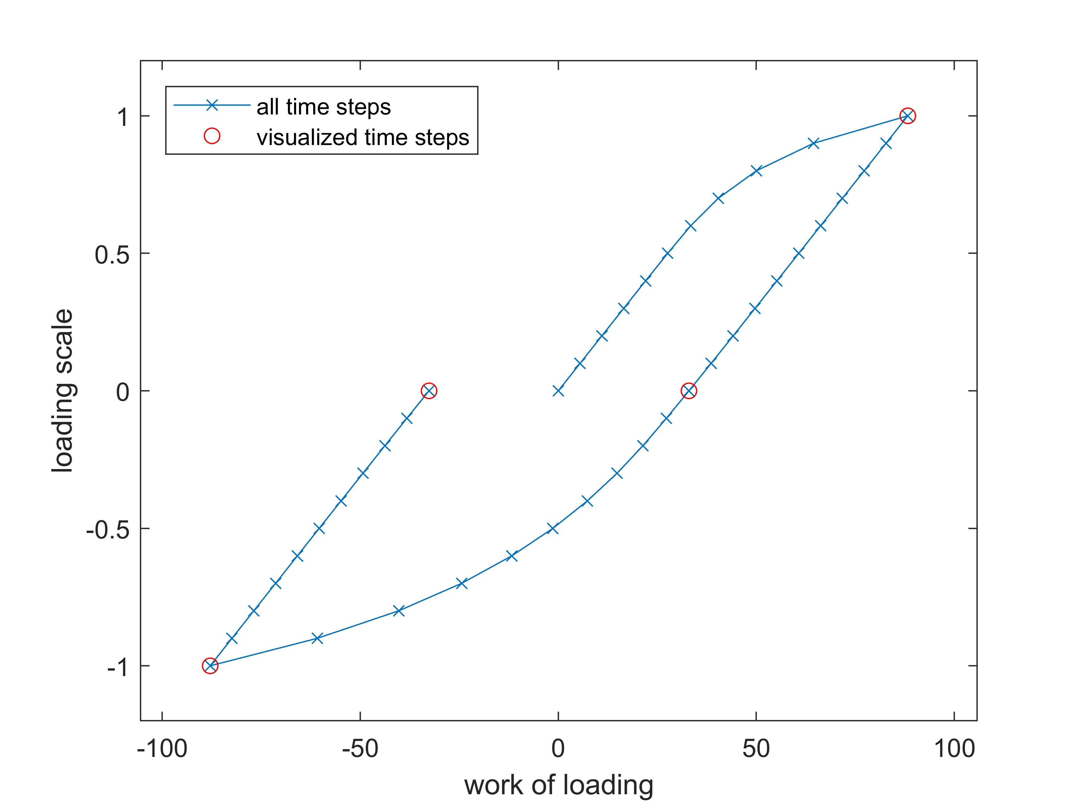
We consider the same geometry as in Section 8.1, see Figure 2. Unlike elasticity, we do not consider the volume force and the nonhomogeneous Dirichlet boundary condition. The traction force prescribed on the upper side is now time dependent, see Figure 4. So the traction force is of the form , , where the scale of external forces varies from to , and . The inelastic material parameters are set as follows: and .
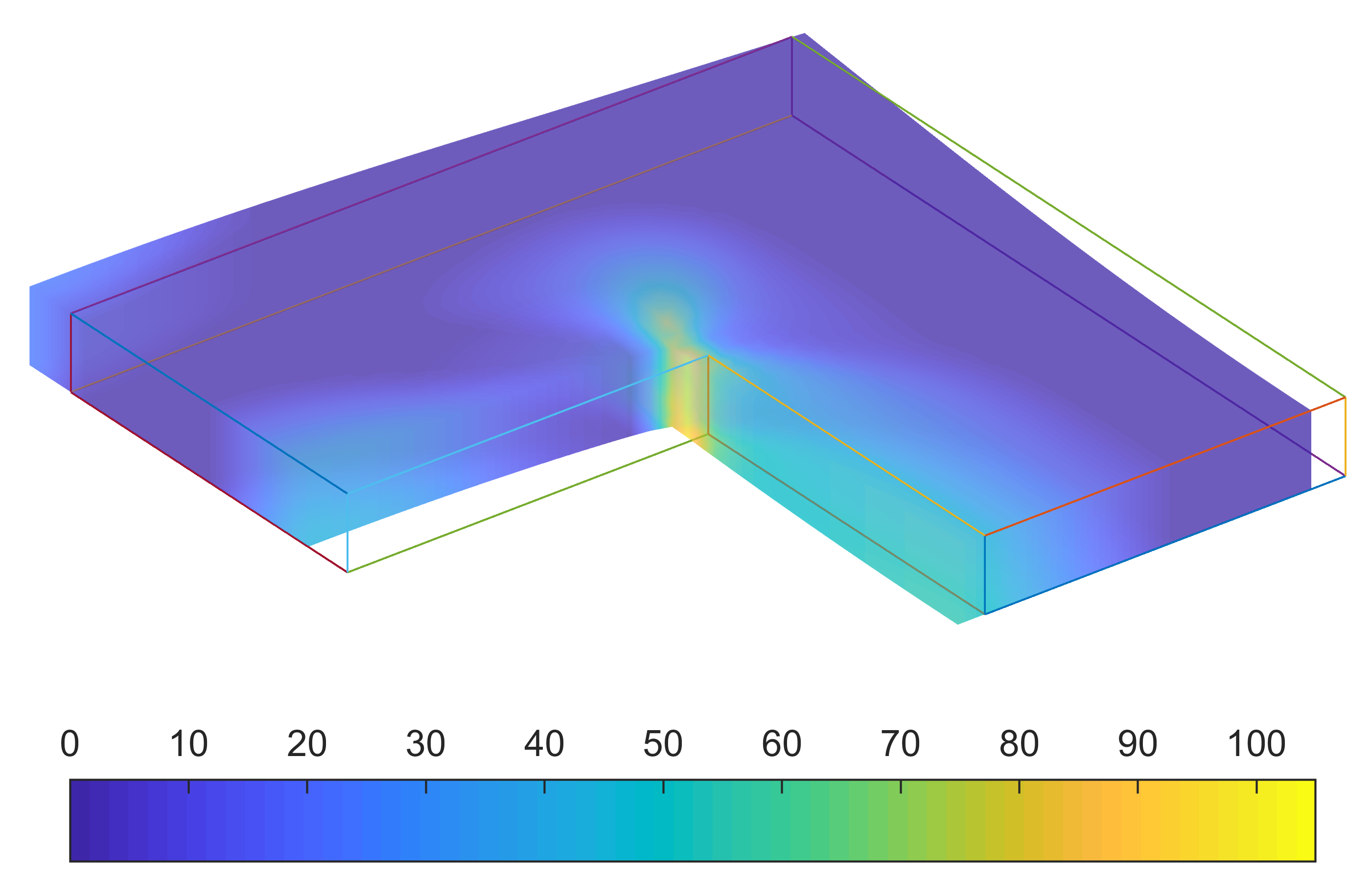
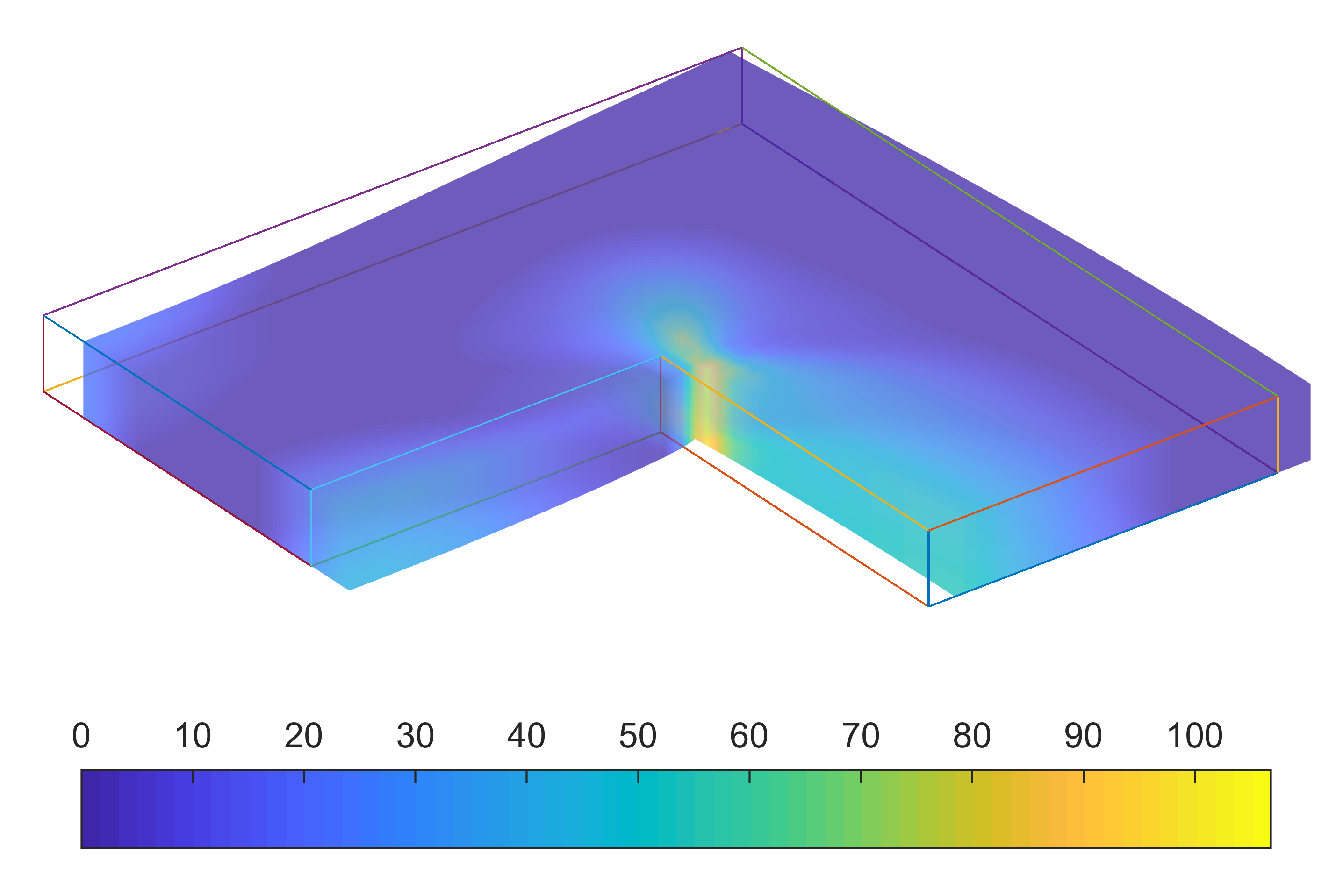
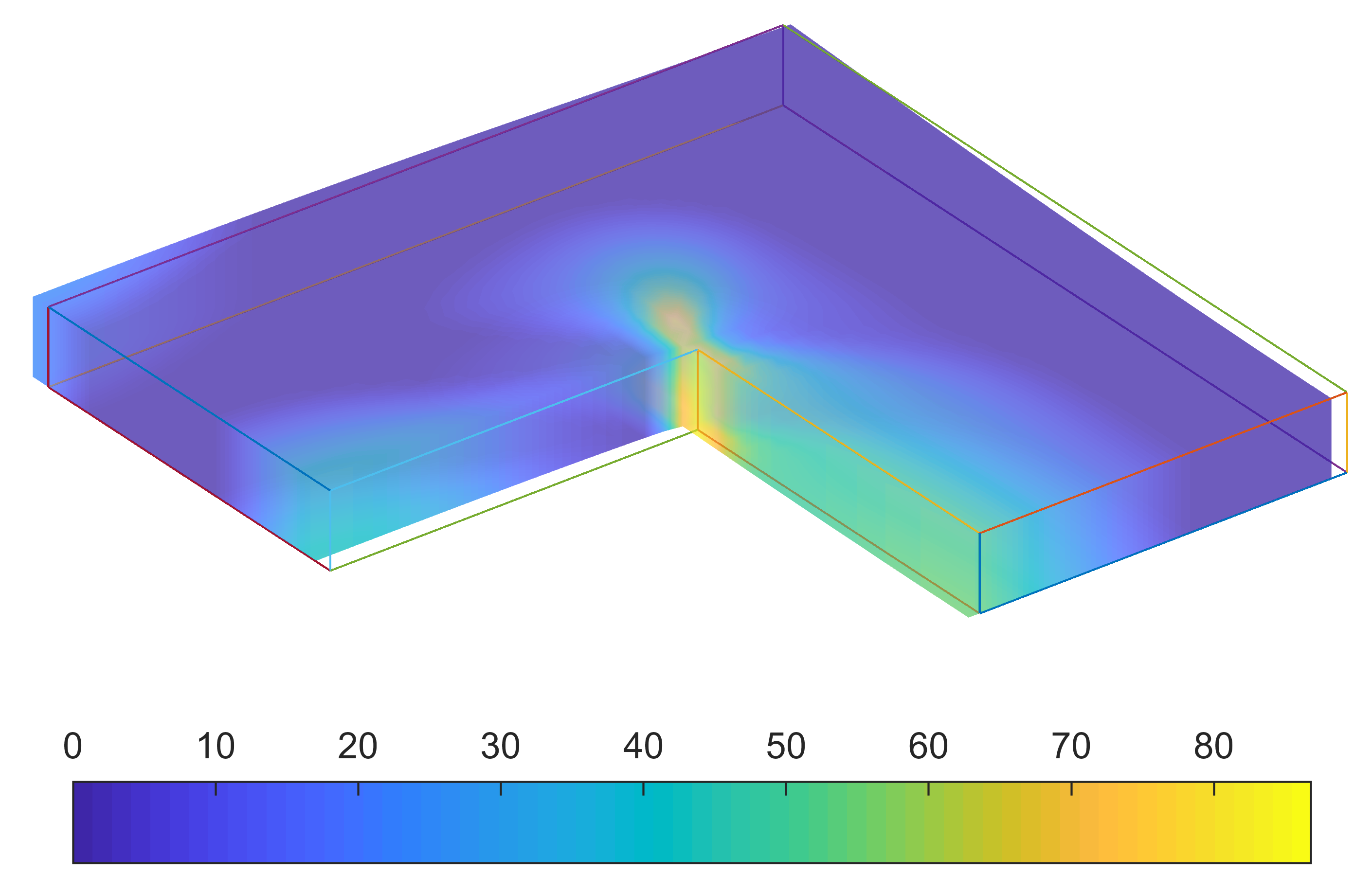
Elastoplasticity related codes are located in directory plasticity and a sequence of incremental steps using von Mises criterion is solved by the script
plasticity_VM_fem;
located in subdirectories plasticity_VM_2D and plasticity_VM_3D. In each step, few iterations of the semismooth Newton method are performed until the convergence is
reached.
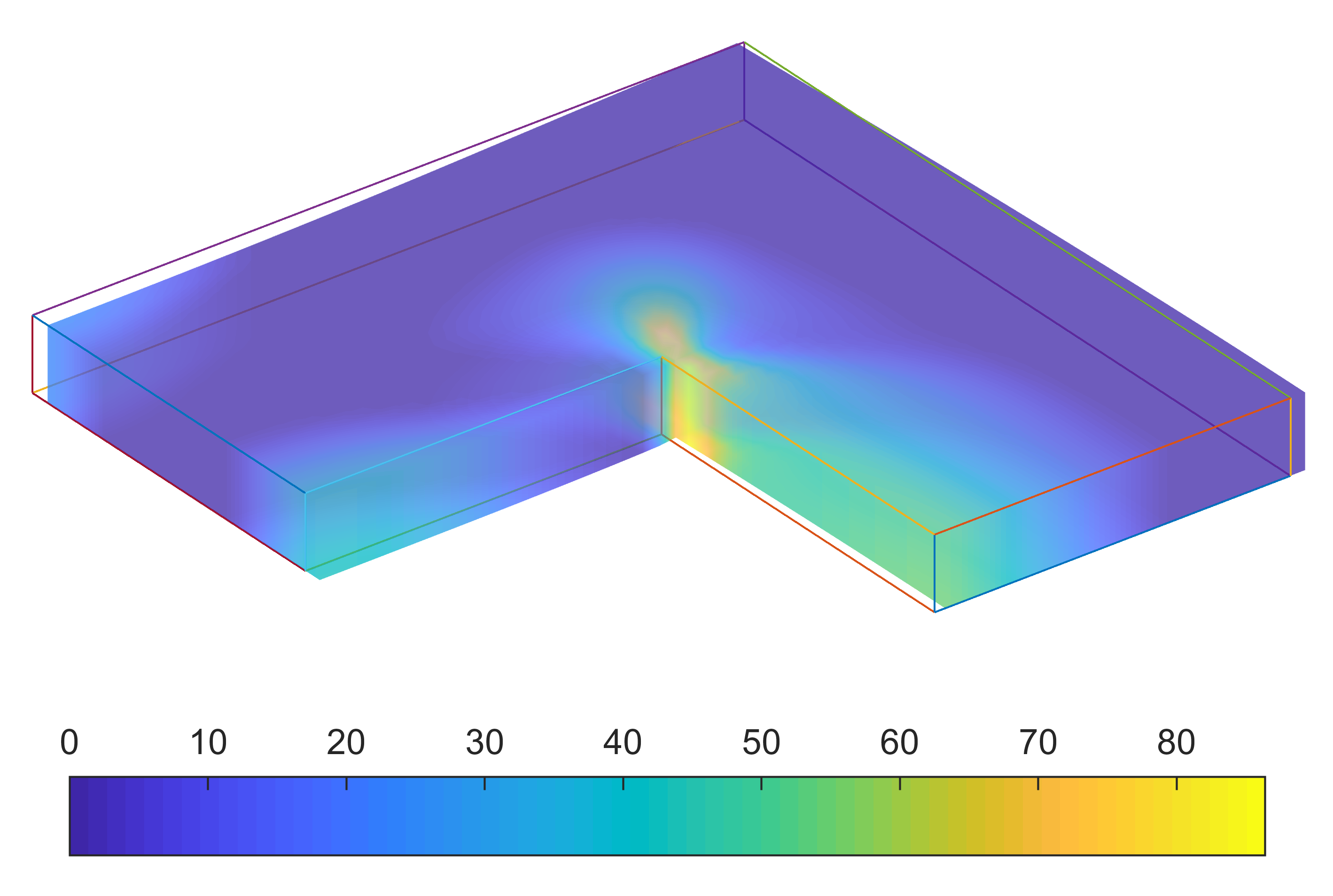
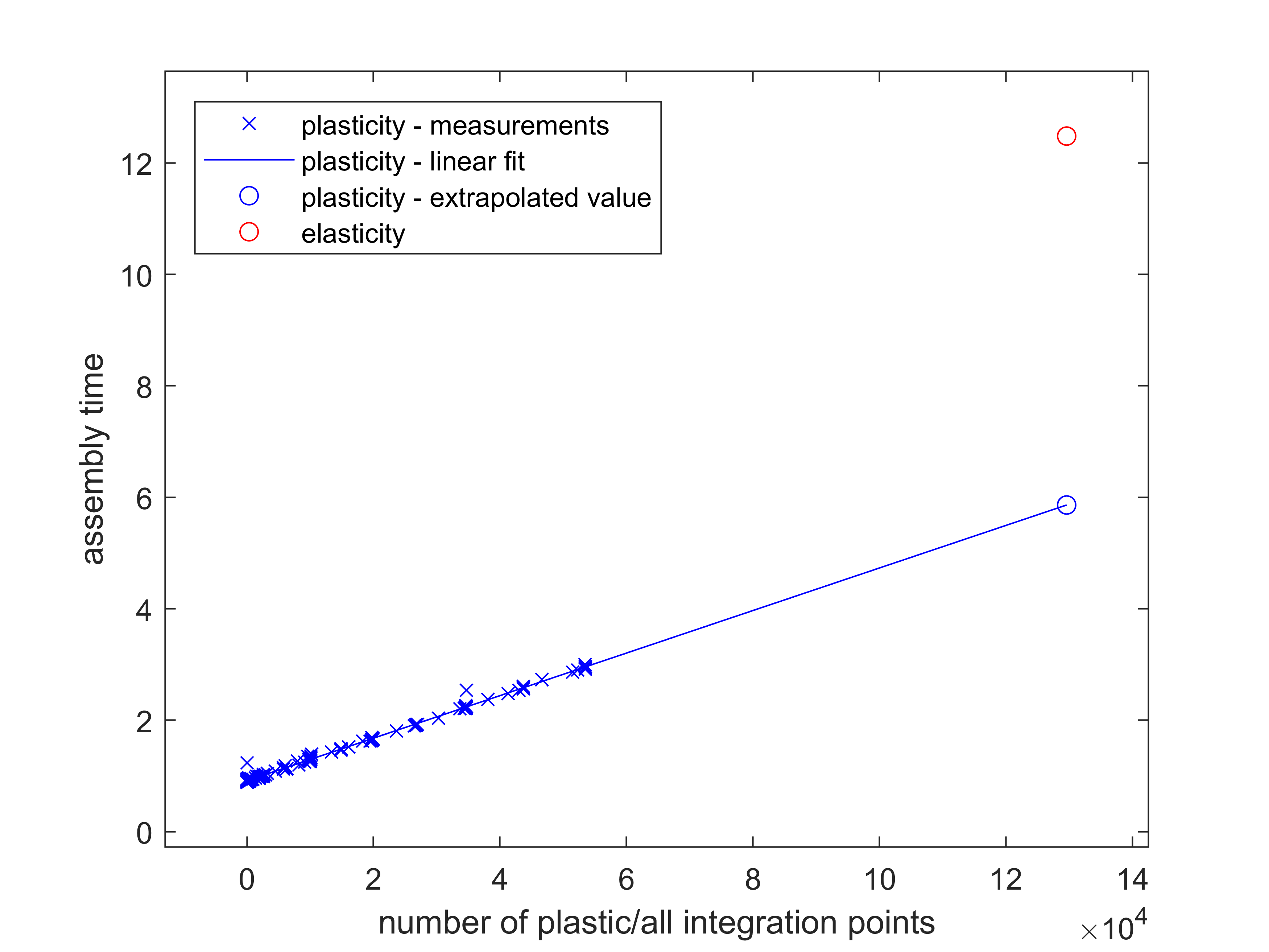
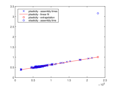
We visualize the results for Q2 elements and the mesh with 23,929 nodes (level 2). Figure 6 depicts hardening fields for Q2 elements in selected time steps. Assembly times of the tangential stiffness matrix in each Newton iteration are stored together with the number of integration points in the plastic regime. Results are displayed in Figure 6. There is a linear relation between the assembly times and the numbers of integration points in the plastic regime. The elastic stiffness matrix is precomputed and its assembly time is not added to measured times. The extrapolated value suggests if all integration points are in the plastic regime, the assembly takes half the time of the elastic matrix assembly in the worst case. Additionally, we also show a hysteresis curve in the same figure as a relation of the scale of external forces and the work of external forces. The work is computed as , where is a vector representing the maximal traction force and is a solution of discretized problem at th time step.
8.3 Assembly of plastic stiffness matrices for the Drucker-Prager yield criterion
An example of computations with Drucker-Prager criterion is available in the script
plasticity_DP_fem;
located in subdirectories plasticity_DP_2D and plasticity_DP_3D. It simulates a well know strip-footing benchmark [7, Chapters 7,8] leading to bearing capacity (limit load) of a soil foundation.
The geometry in plane is depicted in Figure 7. A geometry for the corresponding 3D problem arises from the extrusion in direction of length one. On the left, right and bottom sides of the depicted domain, the zeroth normal displacements are prescribed, i.e., where is a unit normal vector to the boundary. The strip-footing of the length one is considered on the top of the domain. The loading is controlled by the nonhomogeneous Dirichlet boundary condition in the direction . The values varies from 0 to 1 using a suitable adaptive strategy described below. Volume and traction forces are not prescribed. Material parameters are set as follows: (Young’s modulus), (Poisson’s ratio), (cohesion), and (friction angle). The parameters and introduced in Section 2.3 are computed by the following formulas [7, Chapter 6]:
We start with the constant increment . For the solution , we compute the corresponding (average) pressure supported by the footing. It is well known that values of are bounded from above by an unknown limit value. So if we observe that the increment is sufficiently small then we multiply the increment by factor two to achieve the prescribed maximal displacement faster.
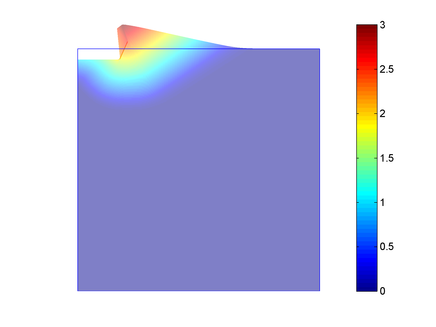
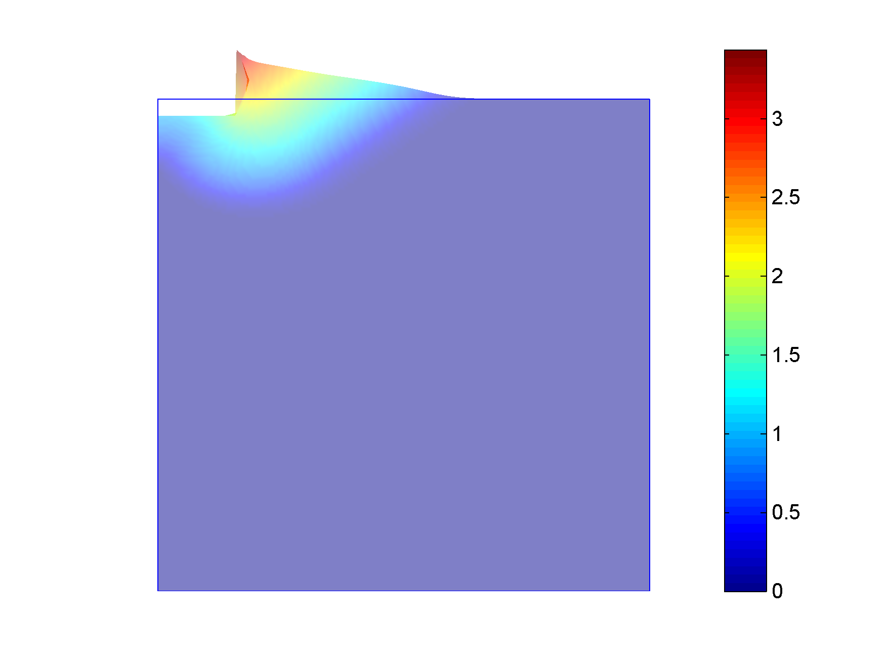
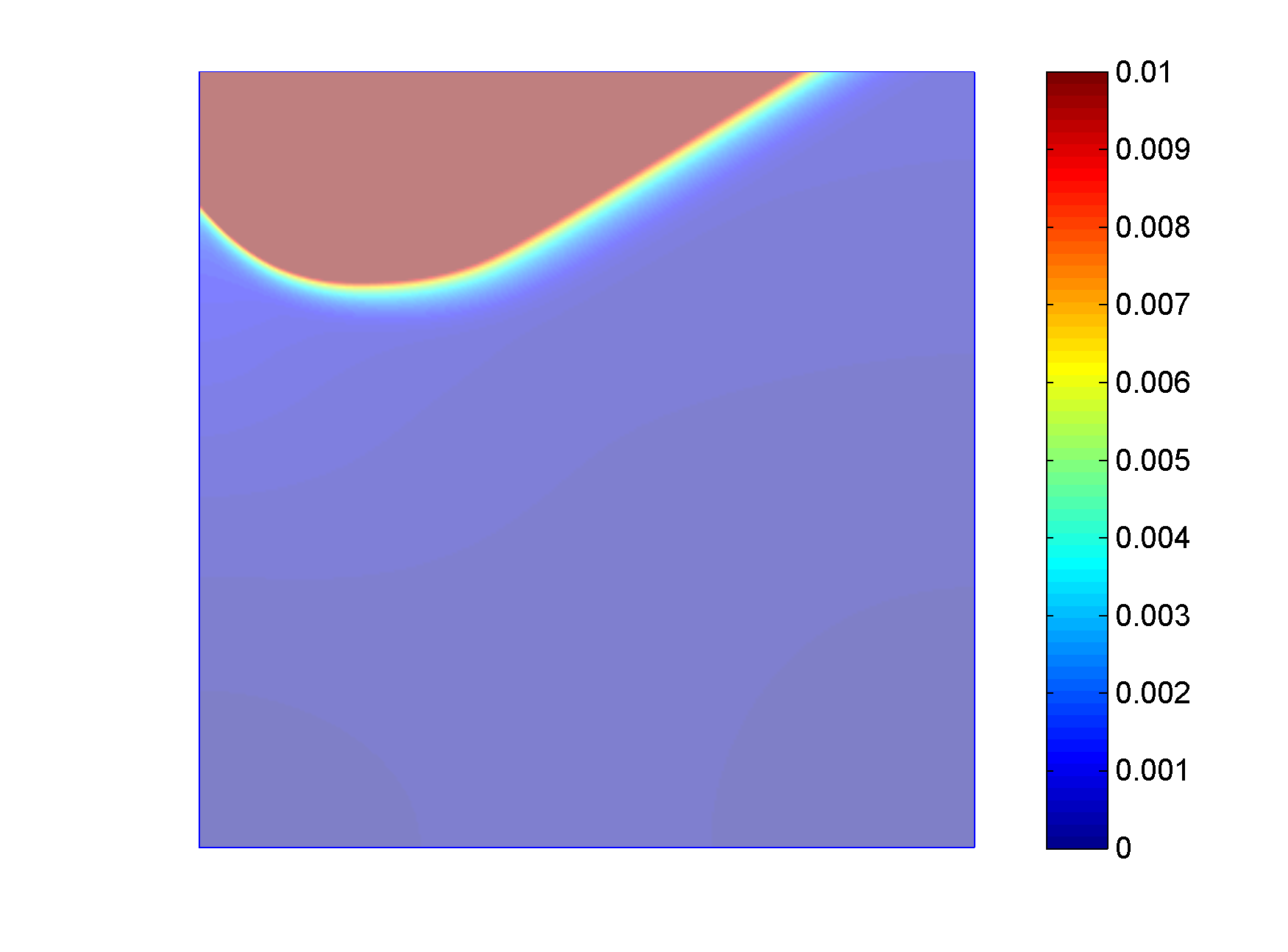
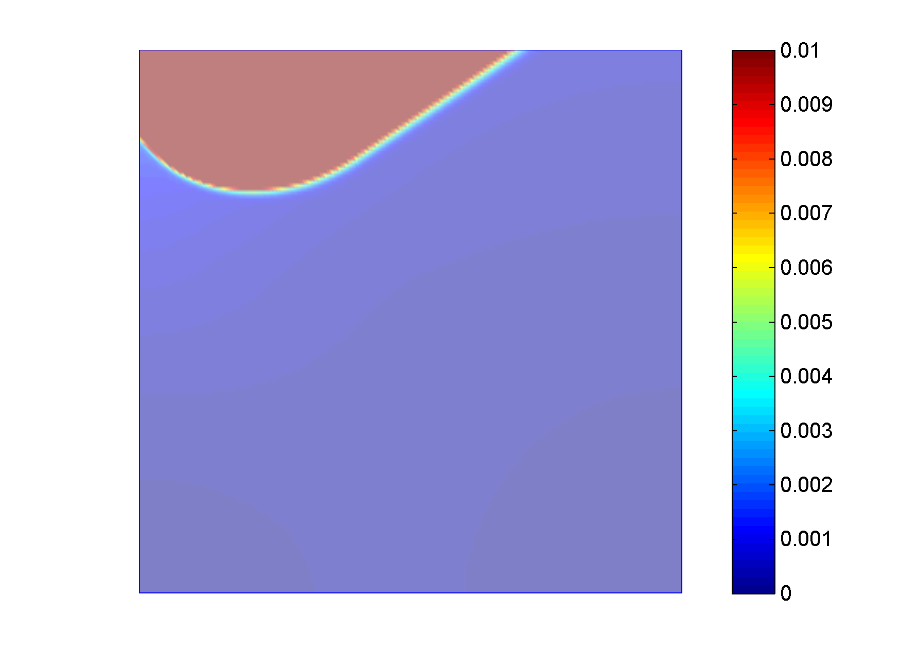
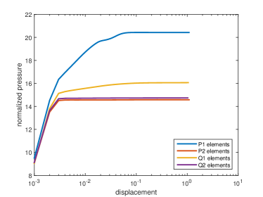
Since the expected results are strongly dependent on the mesh density and on chosen element types, we present the results for 2D problem to achieve finer meshes easily. In particular, we use regular meshes divided the domain into 320320 squares for P1 and Q1 elements, respectively 160160 squares for P2 and Q2 elements to have a similar number of unknowns. Figures 10 and 10 compare plastic collapse for P1 and P2 elements. In Figure 10, we see total displacement fields with deform shapes. To visualize expected slip surfaces, values of displacements greater than are replaced with , see Figure 10. The strong dependence on element types is illustrated in Figure 10 (left). We see that the normalized pressures are significantly overestimated for P1 and Q1 elements. The results for P2 and Q2 elements are in accordance with [7, Chapter 8]. The assembly times of the tangent stiffness matrices are also illustrated in Figure 10 (right). We have a similar observation as for the von Mises yield criterion.
9 Comment on the technique of P. Byczanski
Although the basic split of the tangential stiffness matrix (1) can be written as
| (30) |
this simpler form is not convenient in MATLAB since the difference of sparse matrices and can be much sparser than . This occurs when most of integration points remains in the elastic phase. Therefore, for problems with smaller plastic regions, the assembly of the tangential stiffness matrix can be significantly faster than for problems with larger plastic regions. Let us note that (30) was originally used in unpublished codes from P. Byczanski (UGN Ostrava) applied in numerical examples from [17, 10, 11, 20, 21], but this idea has not been neither emphasized nor described.
10 Conclusion and future plans
The paper is focused on an efficient and flexible implementation of various elastoplastic problems. We have mainly proposed the innovative MATLAB assembly of elastoplastic FEM matrices based on the split (1). Our techniques are explained and implemented in the vectorized code available for download [6]. Time performance of FEM assembly is comparable with other techniques for purely elastic stiffness matrices. Additional effort to build the tangential stiffness matrices in each Newton iteration and each time step of elastoplastic problems does not exceed the cost for the elastic stiffness matrix. The smaller is the number of the plastic integrations points, the faster is the assembly. The code is flexible due to the fact that one can choose several types of (Lagrange) finite elements. It can be further extended for various elastoplastic models by changing the function constitutive_problem.
Acknowledgement. We would like to thank to our former colleague Petr Byczanski (Ostrava) whose ideas inspired this work. The first two authors acknowledge a support from The Ministry of Education, Youth and Sports of the Czech Republic - project LO1404 - Sustainable development of CENET ”CZ.1.05/2.1.00/19.0389: Research Infrastructure Development of the CENET” (the first author); project “IT4Innovations excellence in science - LQ1602” from the National Programme of Sustainability II (the second author). The third author acknowledges a support by the Czech Science Foundation (GAČR) through projects No. 16-34894L, 17-04301S, 18-03834S.
11 Appendix
This appendix completes Section 3 with particular examples of finite elements and related numerical quadratures. We consider P1, P2 tetrahedral elements and Q1, Q2 hexahedral elements for displacement approximation in our implementation. Higher order P- and Q-type elements can be implemented analogously [16]. We recapitulate these elements for 3D case only, see Figure 3 for illustration.
11.1 P1 and P2 tetrahedral elements
The reference P1 element is defined on a reference tetrahedron with 4 nodes
and 4 corresponding linear basis functions (therefore ) are
Notice that strain fields for elements are constant on elements. Therefore, it sufficies to consider 1-point Gauss quadrature, i.e., , and . We see that the weight coefficient coincides with the volume of the reference element.
The reference P2 element is defined on the same reference tetrahedron above with the nodes , , , and also utilizes 6 edges midpoints
Let . Then the quartet defines the barycentric coordinates and one can write the quadratic basis functions as follows:
For P2 elements, we use 11-point numerical quadrature which is exact to order 4. The coordinates of the quadrature points and their weights are following [23]:
11.2 Q1 and Q2 hexahedral elements
The reference Q1 elements is defined on a hexahedron with 8 nodes
and the corresponding linear basis functions () are
We use Gauss quadrature derived from the 1D case where the quadrature points are located at and , and the corresponding weights are equal to one (see [2]).
The reference Q2 element is defined on the same reference hexahedron above and also utilizes 12 edges midpoints
The corresponding quadrature basis functions are defined as follows:
We use Gauss quadrature derived from the 1D case where the quadrature points are located at , , and , and the corresponding weights are equal to 5/9, 8/9, and 5/9, respectively (see [2]).
References
References
- [1] J. Alberty, C. Carstensen, S. A. Funken, and R. Klose. Matlab implementation of the finite element method in elasticity. Computing, 69(3):239–263, 2002.
- [2] K.-J. Bathe. Finite Element Procedures. Klaus-Jürgen Bathe, 2006.
- [3] R. Blaheta. Numerical methods in elasto-plasticity. Peres, 1999.
- [4] M. Carsten C., Brokate and J. Valdman. A quasi-static boundary value problem in multi-surface elastoplasticity. ii: Numerical solution. Mathematical Methods in the Applied Sciences, 28(8):881–901, 2005.
- [5] C. Carstensen and R. Klose. Elastoviscoplastic finite element analysis in 100 lines of Matlab. Journal of Numerical Mathematics, 10(3):157–192, 2002.
- [6] M. Čermák, S. Sysala, and J. Valdman. Matlab FEM package for elastoplasticity. https://github.com/matlabfem/matlab_fem_elastoplasticity, 2018.
- [7] E. A. de Souza Neto, D. Perić, and D. R. J. Owen. Computational Methods for Plasticity. Wiley-Blackwell, 2008.
- [8] P. G. Gruber and J. Valdman. Solution of one-time-step problems in elastoplasticity by a slant Newton method. SIAM Journal on Scientific Computing, 31(2):1558–1580, 2009.
- [9] W. Han and B.D. Reddy. Plasticity: Mathematical Theory and Numerical Analysis. Springer-Verlag, 1999.
- [10] J. Haslinger, S. Repin, and S. Sysala. Guaranteed and computable bounds of the limit load for variational problems with linear growth energy functionals. Applications of Mathematics, 61(5):527–564, 2016.
- [11] J. Haslinger, S. Repin, and S. Sysala. A reliable incremental method of computing the limit load in deformation plasticity based on compliance: Continuous and discrete setting. Journal of Computational and Applied Mathematics, 303:156–170, 2016.
- [12] J. Koko. Fast MATLAB assembly of fem matrices in 2D and 3D using cell-array approach. International Journal of Modeling, Simulation, and Scientific Computing, 7(02):1650010, 2016.
- [13] T. Rahman and J. Valdman. Fast MATLAB assembly of FEM matrices in 2D and 3D: Nodal elements. Applied Mathematics and Computation, 219:7151–7158, 2013.
- [14] M. Sauter and Ch. Wieners. On the superlinear convergence in computational elasto-plasticity. Computer Methods in Applied Mechanics and Engineering, 200(49-52):3646–3658, 2011.
- [15] J. C. Simo and T. J. R. Hughes. Computational Inelasticity. Springer-Verlag, 1998.
- [16] P. Šolín, K. Segeth, and I. Doležel. Higher-order finite element methods, volume 41 of Studies in Advanced Mathematics. Chapman and Hall/CRC, Boca Raton, Florida, 2003.
- [17] S. Sysala. Application of a modified semismooth Newton method to some elasto-plastic problems. Mathematics and Computers in Simulation, 82(10):2004–2021, 2012.
- [18] S. Sysala. Properties and simplifications of constitutive time-discretized elastoplastic operators. ZAMM - Journal of Applied Mathematics and Mechanics / Zeitschrift für Angewandte Mathematik und Mechanik, 94(3):233–255, 2014.
- [19] S. Sysala and M. Čermák. Experimental Matlab code for the slope stability benchmark – SS-DP-AP, SS-DP-NH, SS-JG-P, SS-MC-NP-3D, SS-MC-NH, SS-MC-NP-Acontrol. www.ugn.cas.cz/?p=publish/output.php, 2016. (or www.ugn.cas.cz - Publications - Other outputs - SS-MC-NP-3D, SS-MC-NH, SS-MC-NP-Acontrol).
- [20] S. Sysala, M. Čermák, T. Koudelka, J. Kruis, J. Zeman, and R. Blaheta. Subdifferential-based implicit return-mapping operators in computational plasticity. ZAMM-Journal of Applied Mathematics and Mechanics/Zeitschrift für Angewandte Mathematik und Mechanik, 96(11):1318–1338, 2016.
- [21] S. Sysala, M. Čermák, and T. Ligurský. Subdifferential-based implicit return-mapping operators in Mohr-Coulomb plasticity. ZAMM-Journal of Applied Mathematics and Mechanics/Zeitschrift für Angewandte Mathematik und Mechanik, 97(12), 2017.
- [22] J. Valdman. Two-yield elastoplasticity solver. https://www.mathworks.com/matlabcentral/fileexchange/27246, 2010.
- [23] J. Yu. Symmetric gaussian quadrature formulae for tetrahedronal regions. Computer Methods in Applied Mechanics and Engineering, 43(3):349–353, 1984.