Residual-Based a posteriori error estimation for $hp$-adaptive finite element methods for the Stokes equations

Abstract

We derive a residual-based a posteriori error estimator for the conforming $hp$-Adaptive Finite Element Method ($hp$-AFEM) for the steady state Stokes problem describing the slow motion of an incompressible fluid. This error estimator is obtained by extending the idea of a posteriori error estimation for the classical $h$-version of AFEM. We also establish the reliability and efficiency of the error estimator. The proofs are based on the well-known Clément-type interpolation operator introduced in [28] in the context of the $hp$-AFEM. Numerical experiments show the performance of an adaptive hp-FEM algorithm using the proposed a posteriori error estimator.

1 Introduction

$h$-adaptive finite element methods – in which the mesh size is adjusted to resolve features of the solution – have been known to be efficient tools for solving partial differential equations since the late 1970s [5, 8]. The development of practical and efficient estimators of the local error over the past 25 years [36, 1, 12] has made them a standard tool in the finite element analysis of many equations and is now widely used in applications.

On the other hand, the $p$ or $hp$ versions of adaptive finite element methods – in which one adjusts either the polynomial degree of the approximation on every cell, or both the polynomial degree and the mesh size – has seen much less practical attention. Originally introduced in [9, 6], it is known both theoretically and practically that the $hp$-adaptive FEM can achieve exponential rates of convergence with respect to the number of degrees of freedom [32, 27, 31, 18]. However, it is technically much more complicated to derive reliable and efficient estimates of the error for $hp$ approximations. Furthermore, even once estimates for the error on each cell are available, one is faced with the decision whether increasing the polynomial degree $p$ of the approximation or reducing the mesh size $h$ is more likely to reduce the error, measured with regard to the computational cost of the two possible resulting meshes (see, for example, [22, 37, 20, 30, 2, 25, 16]). Finally, the implementation of algorithms and data structures for conforming $hp$ finite element methods is complex in practice [11].

Furthermore, it has proven to be significantly more difficult to extend many results that are well-established for $h$ adaptivity to $hp$ adaptivity for equations that are not as simple as the Laplace equation. Consequently, published theoretical considerations of error estimates and optimality of refinement strategies are still largely confined to the Laplace equation. Despite the known superiority of $hp$ adaptivity in terms of computational efficiency, its practical impact has therefore not been as profound as $h$-adaptive methods.

In this contribution, we address one of these difficulties by deriving residual-based a posteriori error estimates for conforming $hp$ discretizations of the Stokes equation. This work is inspired by previous work for the Laplace equation [16, 21, 29]. However, it has to address the key difficulty of the Stokes equation that the solution is not the unconstrained minimizer of an energy. Therefore, the Stokes operator is not positive definite, so that working with it is not as straightforward as for example with elliptic operators with their implied coercivity condition.

In particular, we present the following results:

• We derive estimates for the error between the finite-dimensional $hp$ approximation and the continuous solution of the Stokes equation.

• As in similar approaches for the Laplace equation, it is not easily possible to show that these estimates are reliable and efficient, i.e., that the true error is bounded from above and below by our estimator up to a constant that does not depend on $h$ or $p$. This is so because the inverse estimates that are used to derive reliability and efficiency statements typically involve the polynomial degree $p$. To overcome this deficiency, we instead introduce a whole family of estimates $\eta_{\alpha}$ parameterized by an index $\alpha\in[0,1]$. For a fixed $\alpha$, we can not show that an estimator is both efficient and reliable; on the other hand, we can show that for some members of this family, either one or the other property hold. However, we demonstrate through numerical experiments that our estimator for a given $\alpha$ is, in practice, indeed both reliable and efficient.

• We devise a strategy to mark cells for either $h$ or $p$ refinement based on criteria for a systematic reduction of the error.

• Although we make no claims about the optimality of this strategy – i.e., we can not prove that among all strategies it leads to the greatest error reduction – we show numerical results that suggest that the strategy can achieve the desired exponential convergence rate for the $hp$-adaptive refinement.

To the best of our knowledge, none of these properties have previously been derived or demonstrated for the Stokes equation using continuous $hp$-adaptive finite element methods. (However, some related work for discontinuous Galerkin discretizations of the Stokes equations is available in [26].)

The outline of the remainder of this paper is as follows: In Section 2, we introduce the Stokes problem, its weak formulation and the conforming discretization with which we intend to solve it computationally. In Section 3, we introduce necessary notation and state our assumptions as well as some important theoretical results (such as the Clément interpolation operator and polynomial inverse estimates) on which we rely throughout this work. The main results are derived in Section 4, where we develop an $hp$ residual-based a posteriori error estimator for the Stokes problem, followed by the analysis of the reliability and the efficiency of our error estimator. In Section 5 we discuss the details of our $hp$ algorithm, i.e., the criterion upon which we choose either $h$ or $p$ refinement. Finally in Section 6 we present numerical results and demonstrate the performance of the proposed error estimators using practical examples.

2 The Stokes problem and basic assumptions

Let $\Omega\in\mathbb{R}^{\text{2}}$ be an open and connected domain with smooth boundary $\Gamma=\partial\Omega$ such that it satisfies a Lipschitz condition. $u(\text{x})$ is the velocity and $\varrho(\text{x})$ be the pressure of the fluid at some point $\text{x}\in\Omega$, respectively.

Given body forces $f\in L^{2}(\Omega)^{\text{2}}$ and the constant viscosity parameter $\nu>0$, consider stationary incompressible fluid flow as our model problem: For the Stokes equations, we are interested in finding $u:\Omega\to\mathbb{R}^{\text{2}}$ and $\varrho:\Omega\to\mathbb{R}$ such that

$$\begin{split}-\nu\Delta u+\nabla\varrho&=f\qquad\text{in }\enspace\Omega,\\ -\nabla\cdot u&=0\qquad\text{in }\enspace\Omega,\\ u&=0\qquad\text{on }\enspace\Gamma.\end{split}$$ (1)

For ease of presentation, we here assume homogenous no slip boundary condition on the velocity field. (However, similar results as the ones shown herein are also valid for other type of boundary conditions.) To ensure uniqueness of solution, we require vanishing mean for pressure field, i.e., that $\int_{\Omega}\varrho=0$. Here and below, we limit ourselves to the two-dimensional case primarily because Lemmas 1 and 2 below are only available for this case; however, we expect that with additional work, all main results herein could also be shown to hold in three space dimensions.

We denote the standard Sobolev spaces by $H^{m}(\Omega)$ for $m\in\mathbb{N}_{0}$. In particular, the norm and the scalar product of $L^{2}(\Omega)=H^{0}(\Omega)$ are denoted by $\|\cdot\|_{\Omega}$ and $(\cdot,\cdot)_{\Omega}$, respectively. To account for homogeneous Dirichlet boundary conditions, we set

$$H_{0}^{1}(\Omega):=\{v\in H^{1}(\Omega):\varphi=0\text{ on }\Gamma\}.$$

Further, we denote the space containing all functions in $L^{2}(\Omega)$ with zero mean value by

$$L_{0}^{2}(\Omega):=\{v\in L^{2}(\Omega):(\varphi,1)_{\Omega}=0\}$$

and define

$$\mathcal{H}(\Omega):=H_{0}^{1}(\Omega)^{\text{2}}\times L_{0}^{2}(\Omega).$$

Then, we introduce the bilinear form $\mathcal{L}:\mathcal{H}(\Omega)\times\mathcal{H}(\Omega)\to\mathbb{R}$ by

$$\mathcal{L}([u,\varrho];[v,q]):=(\nu\nabla u,\nabla v)_{\Omega}-(\varrho,\nabla\cdot v)_{\Omega}-(\nabla\cdot u,q)_{\Omega}.$$ (2)

The weak formulation of problem (1) then seeks $[u,\varrho]\in\mathcal{H}$ so that

$$\mathcal{L}([u,\varrho];[v,q])=(f,v)_{\Omega}\qquad\forall[v,q]\in\mathcal{H}(\Omega).$$ (3)

Due to the continuous $\inf$-$\sup$ condition

$$\inf_{[u,\varrho]\in\mathcal{H}}\sup_{[v,q]\in\mathcal{H}}\frac{\mathcal{L}([u,\varrho];[v,q])}{\left(\|\nabla u\|_{\Omega}+\|\varrho\|_{\Omega}\right)\left(\|\nabla v\|_{\Omega}+\|q\|_{\Omega}\right)}\geq\kappa>0,$$

where $\kappa$ is the $\inf$-$\sup$ constant depending only on $\Omega$, the weak problem is well-posed and has a unique solution, see [14] and [24].

Now, assume $\mathcal{T}=\{K\}$ is a triangulation of domain $\Omega$. For each element $K$, we associate an element map $T_{K}:\hat{K}\to K$ where the reference cell is $\hat{K}=[0,1]^{\text{2}}$. Further, we define the mesh size vector $h:=\left(h_{K}\right)_{K\in\mathcal{T}},$ where $h_{K}:=\operatorname{diam}(K)$. With each element $K\in\mathcal{T}$, we associate a polynomial degree $p_{K}\in\mathbb{N}$ and collect them in a polynomial degree vector $p:=\left(p_{K}\right)_{K\in\mathcal{T}}$. Throughout this work, we assume that the discretization $(\mathcal{T},p)$ of $\Omega$ is $\left(\gamma_{h},\gamma_{p}\right)$-regular [32, 34].

Definition 1 ($\left(\gamma_{h},\gamma_{p}\right)$-Regularity).

A discretization $(\mathcal{T},p)$ is called $\left(\gamma_{h},\gamma_{p}\right)$-regular if and only if there exist constants $\gamma_{h},\gamma_{p}>0$ such that for all $K,K^{\prime}\in\mathcal{T}$ with $\overline{K}\cap\overline{K^{\prime}}\neq\emptyset$ there holds

$$\gamma_{h}^{-1}h_{K}\leq h_{K^{\prime}}\leq\gamma_{h}h_{K},\qquad\text{and}\qquad\gamma_{p}^{-1}p_{K}\leq p_{K}^{\prime}\leq\gamma_{p}p_{K}.$$ (4)

In other words, the condition implies that the element sizes and also the polynomial degrees of neighboring elements are comparable.

To define the discrete solution space, for an element $K\in\mathcal{T}$ denote $\mathcal{F}(K)$ the set of all interior faces of cell $K$. Then, define by $h_{f}:=\operatorname{diam}(f)$ the diameter of face $f\in\cal F(K)$ and by $p_{f}:=\max\left\{p_{K},p_{K^{\prime}}\right\}$ its polynomial degree where for $K,K^{\prime}\in\mathcal{T}$ are the cells adjacent to $f$. Further, the problem is discretized by the standard $(p_{k},p_{k-1})$ Taylor-Hood finite element. The corresponding $hp$ spaces for velocity and pressure are then

$$V^{p}_{u}(\mathcal{T})^{2} :=\left\{u\in H_{0}^{1}(\Omega)^{2}:\enspace u|_{K}\circ T_{K}\in\mathcal{Q}_{p_{K}}^{2}\left(\hat{K}\right)\text{ for all }K\in\mathcal{T}\right\},$$ (5)

$$V^{p}_{\varrho}(\mathcal{T}) :=\left\{\varrho\in L_{0}^{2}(\Omega):\enspace\varrho|_{K}\circ T_{K}\in\mathcal{Q}_{p_{K}-1}\left(\hat{K}\right)\text{ for all }K\in\mathcal{T}\right\}$$ (6)

$$\mathcal{V}^{p}(\mathcal{T}) :=V_{u}^{p}(\mathcal{T})^{2}\times V_{\varrho}^{p}(\mathcal{T})\subseteq\mathcal{H}(\Omega).$$ (7)

Here, $\mathcal{Q}_{r}$ is the tensor-product polynomial space of complete degree at most $r\in\mathbb{N}_{0}$. Then, the discrete approximation to (3) consists of seeking $\left[u_{\text{FE}},\varrho_{\text{FE}}\right]\in\mathcal{V}^{p}(\mathcal{T})$ such that

$$\mathcal{L}\left(\left[u_{\text{FE}},\varrho_{\text{FE}}\right];\left[v_{\text{FE}},q_{\text{FE}}\right]\right)=\left(f,v_{\text{FE}}\right)_{\Omega}\qquad\forall\left[v_{\text{FE}},q_{\text{FE}}\right]\in\mathcal{V}^{p}(\mathcal{T}).$$ (8)

This choice of spaces satisfies the discrete Babuska-Brezzi condition [4]

$$\inf_{[u_{h},\varrho_{h}]\in\cal{H}}\sup_{[v_{h},q_{h}]\in\cal{H}}\frac{\mathcal{L}([u_{h},\varrho_{h}];[v_{h},q_{h}])}{\left(\|\nabla u_{h}\|+\|\varrho_{h}\|\right)\left(\|\nabla v_{h}\|+\|q_{h}\|\right)}\geq\kappa_{d}>0,$$

where the constant $\kappa_{d}$ is independent of cell size $h$ and polynomial degree $p$. Consequently, problem (8) is well posed.

Furthermore, Galerkin orthogonality holds: Let $[u,\varrho]\in\mathcal{H}$ be the solution of (3) and $\left[u_{\text{FE}},\varrho_{\text{FE}}\right]\in\mathcal{V}^{p}(\mathcal{T})$ be the solution of (8), then

$$\mathcal{L}\left(\left[u-u_{\text{FE}},\varrho-\varrho_{\text{FE}}\right];[v_{\text{FE}},q_{\text{FE}}]\right)=0\qquad\forall\left[v_{\text{FE}},q_{\text{FE}}\right]\in\mathcal{V}^{p}(\mathcal{T}).$$ (9)

3 Auxiliary results

We provide some auxiliary results which we use later in our work. This includes an $H^{1}$-conforming interpolation operator that preserves homogeneous Dirichlet boundary conditions, and some polynomial smoothing estimates. The $H^{1}$-conforming interpolation operator is a Clément-type interpolation which replaces point evaluation by a local average [17]. The procedure does not require the extra regularity of the point evaluation, and is consequently well-defined for functions in $H^{1}(\Omega)$. In [33], this interpolation operator was modified in such a way that it also preserves polynomial boundary conditions. Melenk in [28] extended the aforementioned $H^{1}$-conforming interpolation to the context of $hp$-adaptive finite element spaces.
In our definition of $hp$-Clément interpolation operators, consider $\mathcal{T}$ as a $(\gamma_{h},\gamma_{p})$-regular triangulation of $\mathbb{R}^{\text{d}}$. (For cases where we would want to impose Dirichlet boundary conditions on only a subset $\Gamma_{D}\subset\Gamma$, we can require that $\Gamma_{D}$ can be exactly represented by a collection of faces, i.e., $\bar{\Gamma}_{D}=\cup_{K\in\cal{T}}\partial K\cap\bar{\Gamma}_{D}$.) Then, for a cell $K\in\mathcal{T}$ and a face $f\in\mathcal{F}(K)$ we define the patch sets

$$\omega_{K} :=K\cup\bigcup\{L\in\mathcal{T}:\text{$L$ shares a common edge with $K$}\},$$ (10)

$$\omega_{f} :=\bigcup\{L\in\mathcal{T}:\text{$f$ is an edge of $L$}\}.$$ (11)

The following result from [29] then provides an estimate for the interpolation error in terms of the gradient of the interpolated function:

Theorem 1 ($H^{1}$-Conforming Interpolation).

Let $\mathcal{T}$ be $\left(\gamma_{h},\gamma_{p}\right)$-regular and $K\in\mathcal{T}$ be arbitrary. Then, there exists a bounded linear operator $\Pi^{hp}:H_{0}^{1}(\Omega)^{2}\to\mathcal{V}^{p}(\mathcal{T})$ – namely, the Clément interpolation operator –, and a constant $C>0$ independent of mesh size $h$ and polynomial degree $p$ such that for all $u\in H_{0}^{1}(\Omega)$ and all $f\in\mathcal{F}(K)$

$$\left\|u-\Pi^{hp}u\right\|_{L^{2}(K)} \leq C\frac{h_{K}}{p_{K}}\|\nabla u\|_{L^{2}({\omega_{K}})},$$ (12)

$$\left\|u-\Pi^{hp}u\right\|_{L^{2}(f)} \leq C\sqrt{\frac{h_{f}}{p_{f}}}\|\nabla u\|_{L^{2}({\omega_{f}})}.$$ (13)

Proof.

Following the lines of [32], one can find proofs in [28, Theorem 3.3]. ∎

Next, let us present some polynomial smoothing estimates that are widely used in the error analysis of many numerical methods for partial differential equations and integral equations [13, 29]. We will later use them in proving upper and lower bounds of our error estimator. Specifically, define the smoothing weight functions $\Phi_{K}:K\subset\mathbb{R}^{2}\to\mathbb{R}^{+}$ and $\Phi_{\omega_{f}}:\omega_{f}\subset\mathbb{R}^{2}\to\mathbb{R}^{+}$ by

$$\Phi_{K}(x) :=\frac{1}{h_{K}}\operatorname{dist}\left(x,\partial K\right),$$ (14)

$$\Phi_{\omega_{f}}(x) :=\frac{1}{\text{diam}(\omega_{f})}\text{dist}(x,\partial\omega_{f}).$$ (15)

Then we have:

Lemma 1.

Let $\delta\in[0,1]$, $a,b\in\mathbb{R}$ such that $-1\leq a\leq b$. Then, for any $\pi_{p}\in\mathcal{Q}_{p}\left(K\right)$, there exists some constant $C>0$ independent of $h$ and $p$ so that

$$\|\pi_{p}\left(\Phi_{K}\right)^{a}\|_{\text{L}^{2}(K)} \leq C(a,b)p^{(b-a)}\|\pi_{p}\left(\Phi_{K}\right)^{b}\|_{\text{L}^{2}(K)},$$ (16)

$$\|\nabla\pi_{p}\left(\Phi_{K}\right)^{\delta}\|_{\text{L}^{2}(K)} \leq\frac{C(\delta)p^{(2-\delta)}}{h_{K}}\|\pi_{p}\left(\Phi_{K}\right)^{\frac{\delta}{2}}\|_{\text{L}^{2}(K)}.$$ (17)

Proof.

See [13, Lemmas 4, 5] and [29, Lemma 2.5]. ∎

The next lemma provides results for the extension of a polynomial from an edge to a domain. These estimates are used in the efficiency analysis of our error estimator.

Lemma 2.

Let $\hat{f}$ be the edge of unit square $\hat{K}$, and $0\leq\alpha\leq 1$. $\Phi_{\omega_{\hat{f}}}$ defined as in (15) the edge $\hat{f}$ corresponding to the unit cell $\hat{K}$. Then there exists $C_{\alpha}>0$, such that for any polynomial $\pi_{p}\in\mathcal{Q}_{p}$ and every $\delta\in(0,1]$, there exists some extension $v_{\hat{f}}\in H_{0}^{1}\left(\hat{K}\right)$ so that:

$$v_{\hat{f}}|_{\hat{f}} =\pi_{p}\Phi_{\omega_{\hat{f}}}^{\alpha},\hskip 3.0ptv_{\hat{f}}|_{\partial\hat{K}\backslash\hat{f}}=0,$$

$$\|v_{\hat{f}}\|_{L^{2}({\hat{K}})}^{2} \leq C_{\alpha}\delta\|\pi_{p}\Phi^{\frac{\alpha}{2}}_{\omega_{\hat{f}}}\|_{L^{2}({\hat{f}})}^{2},$$

$$\|\nabla v_{\hat{f}}\|_{L^{2}(\hat{K})}^{2} \leq C_{\alpha}(\delta p^{2(2-\alpha)}+\delta^{-1})\left\|\pi_{p}\Phi^{\frac{\alpha}{2}}_{\omega_{\hat{f}}}\right\|^{2}_{L^{2}(\hat{f})}.$$

Proof.

See [29, Lemma 2.6]. ∎

4 A posteriori error estimation

A posteriori error estimates assess the error between the exact solution $[u,\varrho]\in\mathcal{H}$ and its finite element approximation $\left[u_{\text{FE}},\varrho_{\text{FE}}\right]\in\mathcal{V}^{p}(\mathcal{T})$ only in terms of known quantities [23, 7, 35] – i.e., the problem data and the approximate solution. We call a functional $\eta\left(u_{\text{FE}},\varrho_{\text{FE}},f\right)$ an a posteriori error estimator for the Stokes equation, if and only if there exists a constant $C>0$ such that

$$\left\|\nabla\left(u-u_{\text{FE}}\right)\right\|_{\Omega}+\left\|\varrho-\varrho_{\text{FE}}\right\|_{\Omega}\leq C\eta\left(u_{\text{FE}},\varrho_{\text{FE}},f\right).$$ (18)

Furthermore, if $\eta\left(u_{\text{FE}},\varrho_{\text{FE}},f\right)$ can be decomposed into localized quantities $\eta_{K}\left(u_{\text{FE}},\varrho_{\text{FE}},f\right)$, $K\in\mathcal{T}$, such that

$$\eta(u_{\text{FE}},\varrho_{\text{FE}},f)^{2}=\sum_{K\in\mathcal{T}}\eta_{K}\left(u_{\text{FE}},\varrho_{\text{FE}},f\right)^{2},$$ (19)

then $\eta_{K}\left(u_{\text{FE}},\varrho_{\text{FE}},f\right)$ is called a local error indicator.

Estimate (18) is usually called a “reliability estimate” since it guarantees that the error is controlled by the error estimator $\eta\left(u_{\text{FE}},\varrho_{\text{FE}},f\right)$ up to a constant independent of mesh size $h$ and polynomial degree $p$. Further, the local error indicators $\eta_{K}\left(u_{\text{FE}},\varrho_{\text{FE}},f\right)$ provides the basis for adaptive mesh refinement by identifying those cells $K\in\mathcal{T}$ where the error is large and that, consequently, should be refined locally. This procedure is then repeated until $\eta\left(u_{\text{FE}},\varrho_{\text{FE}},f\right)$ is smaller than a prescribed tolerance.

Computational efficiency requires that the $\eta_{K}$ also satisfy some efficiency property guaranteeing that the upper bound (18) is sharp and does not asymptotically overestimate the true error. To this end, we would like to derive a local lower bound for the energy error for every cell $K\in\mathcal{T}$:

$$\eta_{K}\left(u_{\text{FE}},\varrho_{\text{FE}},f\right)\leq C\left(\left\|\nabla\left(u-u_{\text{FE}}\right)\right\|^{2}_{\omega_{K}}+\left\|\varrho-\varrho_{\text{FE}}\right\|^{2}_{\omega_{K}}\right)^{1/2}.$$ (20)

4.1 Residual-based a posteriori error analysis

Let us now define a residual-based a posteriori error estimator for problem (1), and derive upper and lower bounds for it in terms of the energy error of the approximated solution. In the spirit of [29], we define a family of error estimators $\eta_{\alpha}$, $\alpha\in[0,1]$. This estimator is local, i.e., $\eta_{\alpha}^{2}:=\sum_{K\in\mathcal{T}}\eta_{\alpha;K}^{2}$ and can be decomposed into cell and interface contributions:

$$\eta_{\alpha;K}^{2} :=\eta_{\alpha;K;R}^{2}+\eta_{\alpha;K;B}^{2},$$ (21)

$$\eta_{\alpha;K;R}^{2} :=\frac{h_{K}^{2}}{p_{K}^{2}}\left\|\left(I_{p_{K}}^{K}f+\nu\Delta u_{\text{FE}}-\nabla\varrho_{\text{FE}}\right)\Phi_{K}^{\frac{\alpha}{2}}\right\|^{2}_{K}+\left\|\left(\nabla\cdot u_{\text{FE}}\right)\Phi_{K}^{\frac{\alpha}{2}}\right\|^{2}_{K},$$ (22)

$$\eta_{\alpha;K;B}^{2} :=\sum_{f\in\cal F(K)}\frac{h_{f}}{2p_{f}}\left\|\left[\nu\frac{\partial u_{\text{FE}}}{\partial n_{K}}\right]\Phi_{\omega_{f}}^{\frac{\alpha}{2}}\right\|_{f}^{2}.$$ (23)

Here, $I_{p_{K}}^{K}f$ denotes the local $L^{2}$-projection of $f$ into the space of piecewise polynomials of degree $p_{K}$. Furthermore, $h_{f}:=\text{diam}(f)$ and $p_{f}:=\max(p_{K},p_{K^{\prime}})$ for a face $f$ that is shared by cells $K$ and $K^{\prime}$. Finally, $[\cdot]$ denotes the jump of a quantity across a face whose outward normal relative to $K$ is indicates by $n_{K}$.

In the following, we will first derive an upper bound for the energy error in terms of the estimator $\eta_{\alpha}$, i.e., state a reliability estimate.

Theorem 2 (Reliability).

Let $[u,\varrho]\in\mathcal{H}$ and $\left[u_{\text{FE}},\varrho_{\text{FE}}\right]\in\mathcal{V}^{p}(\mathcal{T})$ be the solutions of (3) and (8), respectively. Further, let $\alpha\in[0,1]$ and assume that triangulation $\mathcal{T}$ is $\left(\gamma_{h},\gamma_{p}\right)$-regular. Then there exists a constant $C_{\text{rel}}>0$ independent of mesh size vector $h$ and polynomial degree vector $p$ such that

$$\left\|\nabla\left(u-u_{\text{FE}}\right)\right\|_{\Omega}^{2}+\left\|\varrho-\varrho_{\text{FE}}\right\|_{\Omega}^{2}\leq C_{\text{rel}}\sum_{K\in\mathcal{T}}\left(p_{K}^{2\alpha}\eta_{\alpha;K}^{2}+\frac{h_{K}^{2}}{p_{K}^{2}}\left\|I_{p_{K}}^{K}f-f\right\|^{2}_{K}\right).$$

In particular, the statement provides a $p$-independent reliability bound for $\alpha=0$.

Proof.

Set $e_{\text{FE}}:=u-u_{\text{FE}}$ and $\epsilon_{\text{FE}}:=\varrho-\varrho_{\text{FE}}$. From (9), we have

$$\mathcal{L}\left(\left[e_{\text{FE}},\epsilon_{\text{FE}}\right];[v,q]\right) =\left(\nu\nabla e_{\text{FE}},\nabla\left(v-\Pi^{hp}v\right)\right)_{\Omega}$$

$$\qquad-\left(\epsilon_{\text{FE}},\nabla\cdot\left(v-\Pi^{hp}v\right)\right)_{\Omega}-\left(\nabla\cdot e_{\text{FE}},q\right)_{\Omega}$$

$$=\sum_{K\in\mathcal{T}}\bigg{(}\left(\nu\nabla e_{\text{FE}},\nabla\left(v-\Pi^{hp}v\right)\right)_{K}$$

$$\qquad\qquad-\left(\epsilon_{\text{FE}},\nabla\cdot\left(v-\Pi^{hp}v\right)\right)_{K}-\left(\nabla\cdot e_{\text{FE}},q\right)_{K}\bigg{)},$$

where $\Pi^{hp}:H_{0}^{1}(\Omega)^{2}\to\mathcal{V}^{p}(\mathcal{T})$ is the $H^{1}$-conforming interpolation operator from Theorem 1. Using integration by parts and the incompressibility condition $\nabla\cdot u=0$ yields

$$\mathcal{L}\left(\left[e_{\text{FE}},\epsilon_{\text{FE}}\right];[v,q]\right)=\sum_{K\in\mathcal{T}}\Bigg{(}\left(f+\nu\Delta u_{\text{FE}}-\nabla\varrho_{\text{FE}},v-\Pi^{hp}v\right)_{K}\\ -\left(\nabla\cdot u_{\text{FE}},q\right)_{K}+\sum_{f\in\cal F(K)}\left(\left[\nu\frac{\partial u_{\text{FE}}}{\partial n}\right],v-\Pi^{hp}v\right)_{f}\Bigg{)}.$$

The continuous Cauchy-Schwarz inequality then results in the estimate

$$\mathcal{L}\left(\left[e_{\text{FE}},\epsilon_{\text{FE}}\right];[v,q]\right)\leq\sum_{K\in\mathcal{T}}\Bigg{(}\left\|I_{p_{K}}^{K}f+\nu\Delta u_{\text{FE}}-\nabla\varrho_{\text{FE}}\right\|_{K}\left\|v-\Pi^{hp}v\right\|_{K}\\ \qquad\qquad\qquad+\left\|\nabla\cdot u_{\text{FE}}\right\|_{K}\|q\|_{K}+\left\|f-I_{p_{K}}^{K}f\right\|_{K}\left\|v-\Pi^{hp}v\right\|_{K}\\ +\sum_{f\in\cal F(K)}\left\|\left[\nu\frac{\partial u_{\text{FE}}}{\partial n_{K}}\right]\right\|_{f}\left\|v-\Pi^{hp}v\right\|_{f}\Bigg{)}.$$

Theorem 1 allows us to locally bound the differences $v-\Pi^{hp}v$. This yields

$$\begin{split}\mathcal{L}\left(\left[e_{\text{FE}},\epsilon_{\text{FE}}\right];[v,q]\right)&\leq C\sum_{K\in\mathcal{T}}\Bigg{(}\frac{h_{K}}{p_{K}}\left\|I_{p_{K}}^{K}f+\nu\Delta u_{\text{FE}}-\nabla\varrho_{\text{FE}}\right\|_{K}\\ &+\left\|\nabla\cdot u_{\text{FE}}\right\|_{K}+\frac{h_{K}}{p_{K}}\left\|f-I_{p_{K}}^{K}f\right\|_{K}\quad\\ &+\sum_{f\in\cal F(K)}\sqrt{\frac{h_{f}}{p_{f}}}\left\|\left[\nu\frac{\partial u_{\text{FE}}}{\partial n_{K}}\right]\right\|_{f}\Bigg{)}\left(\|\nabla v\|_{\omega_{K}}+\|q\|_{K}\right),\end{split}$$

which we can further estimate as follows:

$$\mathcal{L}\left(\left[e_{\text{FE}},\epsilon_{\text{FE}}\right];[v,q]\right)\\ \leq C\left(\sum_{K\in\mathcal{T}}\left(\eta_{0;K}^{2}+\frac{h_{K}^{2}}{p_{K}^{2}}\left\|f-I_{p_{K}}^{K}f\right\|_{K}^{2}\right)\right)^{\frac{1}{2}}\left(\|\nabla v\|_{\Omega}^{2}+\|q\|_{\Omega}^{2}\right)^{\frac{1}{2}}$$

for some constant $C>0$ independent of mesh size vector $h$ and polynomial degree vector $p$. Moreover, for $(e_{\text{FE}},\varepsilon_{\text{FE}})\in\mathcal{H}$ we have

$$\left(\left\|\nabla e_{\text{FE}}\right\|_{\Omega}^{2}+\left\|\epsilon_{\text{FE}}\right\|_{\Omega}^{2}\right)^{\frac{1}{2}}\leq C\sup_{[v,q]\in\mathcal{H}}\frac{\mathcal{L}\left(\left[e_{\text{FE}},\epsilon_{\text{FE}}\right];[v,q]\right)}{(\|\nabla v\|_{\Omega}^{2}+\|q\|_{\Omega}^{2})^{\frac{1}{2}}},$$

for some constant $C>0$. This implies the claimed result for $\alpha=0$. Using the inverse estimates given in Lemma 1, we can bound $\eta_{0;K}$ in terms of $\eta_{\alpha;K}$ for $\alpha\in(0,1]$ from above. Therefore, setting $a:=0$ and $b:=\alpha$ in Lemma 1 and we get

$$\left(\left\|\nabla e_{\text{FE}}\right\|_{\Omega}^{2}+\left\|\epsilon_{\text{FE}}\right\|_{\Omega}^{2}\right)^{\frac{1}{2}}\leq C_{rel}\left(\sum_{K\in\mathcal{T}}\left(p_{K}^{2\alpha}\eta_{\alpha;K}^{2}+\frac{h_{K}^{2}}{p_{K}^{2}}\left\|f-I_{p_{K}}^{K}f\right\|_{K}^{2}\right)\right)^{\frac{1}{2}}$$

which concludes the proof. ∎

Next, we derive an upper bound for the a posteriori error estimator $\eta_{\alpha;K}$ in terms of the energy error $\left\|\nabla\left(u-u_{\text{FE}}\right)\right\|_{\omega_{K}}^{2}+\left\|\varrho-\varrho_{\text{FE}}\right\|_{\omega_{K}}^{2}$ defined on the patch $\omega_{K}$ around cell $K$. Under mild assumptions on the mesh, this then constitutes an efficiency estimate for the error estimator. We will first consider the residual and jump terms $\eta_{\alpha;K;R},\eta_{\alpha;K;B}$ separately and combine the derived efficiency estimates later to obtain an upper bound for the residual-based a posteriori error estimator from definition (21).

Lemma 1.

Let $[u,\varrho]\in\mathcal{H}$, $\left[u_{\text{FE}},\varrho_{\text{FE}}\right]\in\mathcal{V}^{p}(\mathcal{T})$, and $\mathcal{T}$ as in Theorem 2, and $\alpha\in[0,1]$ be arbitrary. Then, there exists a constant $C>0$ independent of the mesh size vector $h$ and polynomial degree vector $p$ so that

$$\eta_{\alpha;K;R}^{2}\leq C\bigg{(}p_{K}^{2(1-\alpha)}\left(\nu^{2}\left\|\nabla\left(u-u_{\text{FE}}\right)\right\|_{K}^{2}+\left\|\varrho-\varrho_{\text{FE}}\right\|^{2}_{K}\right)\\ +\frac{h_{K}^{2+\frac{\alpha}{2}}}{p_{K}^{1+\alpha}}\left\|f-I^{K}_{p_{K}}f\right\|^{2}_{K}\bigg{)}.$$

In particular, the statement provides a $p$-independent efficiency bound of the cell-residual term for $\alpha=1$.

Proof.

Let us write the residual-based term as $\eta_{\alpha;K;R}^{2}=\eta_{\alpha;K;R_{1}}^{2}+\eta_{\alpha;K;R_{2}}^{2},$ with

$$\begin{split}\eta_{\alpha;K;R_{1}}^{2}&:=\frac{h^{2}_{K}}{p^{2}_{K}}\left\|\left(I^{K}_{p_{K}}f+\nu\Delta u_{\text{FE}}-\nabla\varrho_{\text{FE}}\right)\Phi_{K}^{\frac{\alpha}{2}}\right\|^{2}_{K},\\ \eta_{\alpha;K;R_{2}}^{2}&:=\left\|\nabla\cdot u_{\text{FE}}\Phi_{K}^{\frac{\alpha}{2}}\right\|^{2}_{K}.\end{split}$$ (24)

Using the idea in [29] to build test functions, for $0<\alpha\leq 1$, we define the cell residual term $R_{K}$ as, $R_{K}:=\left(I^{K}_{p_{K}}f+\nu\Delta u_{\text{FE}}-\nabla\varrho_{\text{FE}}\right)\Phi_{K}^{\alpha}\in H_{0}^{1}(K)$ and obtain

$$\left\|R_{K}\Phi_{K}^{-\frac{\alpha}{2}}\right\|^{2}_{K}=\left(f+\nu\Delta u_{\text{FE}}-\nabla\varrho_{\text{FE}},R_{K}\right)_{K}+\left(I^{K}_{p_{K}}f-f,R_{K}\right)_{K}.$$ (25)

With equation (3) and applying integration by parts, the first term reads

$$\left(f+\nu\Delta u_{\text{FE}}-\nabla\varrho_{\text{FE}},R_{K}\right)_{K}\\ =\left(\nu\nabla\left(u-u_{\text{FE}}\right),\nabla R_{K}\right)_{K}-\left(\varrho-\varrho_{\text{FE}},\nabla\cdot R_{K}\right)_{K}-\left(\nabla\cdot u,q\right)_{K}.$$

Inserting into (25) and using that $\nabla\cdot u=0$ implies

$$\left\|R_{K}\Phi_{K}^{-\frac{\alpha}{2}}\right\|^{2}_{K} =\left(\nu\nabla\left(u-u_{\text{FE}}\right),\nabla R_{K}\right)_{K}-\left(\varrho-\varrho_{\text{FE}},\nabla\cdot R_{K}\right)_{K}$$

$$\qquad+\left(I^{K}_{p_{K}}f-f,R_{K}\right)_{K}$$

$$\leq\bigg{(}\nu\left\|\nabla\left(u-u_{\text{FE}}\right)\right\|_{K}+\left\|\varrho-\varrho_{\text{FE}}\right\|_{K}\bigg{)}\left\|\nabla R_{K}\right\|_{K}$$

$$\qquad+\left\|\left(I^{K}_{p_{K}}f-f\right)\Phi_{K}^{\frac{\alpha}{2}}\right\|_{K}\left\|R_{K}\Phi_{K}^{-\frac{\alpha}{2}}\right\|_{K}.$$ (26)

Using equations (16) and (17) in Lemma 1, we can estimate

$$\left\|\nabla R_{K}\right\|_{K}^{2} =\left\|\nabla\bigg{(}\left(I^{K}_{p_{K}}f+\nu\Delta u_{\text{FE}}-\nabla\varrho_{\text{FE}}\right)\Phi_{K}^{\alpha}\bigg{)}\right\|_{K}^{2}$$

$$\leq 2\left\|\nabla\left(I^{K}_{p_{K}}f+\nu\Delta u_{\text{FE}}-\nabla\varrho_{\text{FE}}\right)\Phi_{K}^{\alpha}\right\|^{2}_{K}$$

$$\qquad+2\left\|\left(I^{K}_{p_{K}}f+\nu\Delta u_{\text{FE}}-\nabla\varrho_{\text{FE}}\right)\Phi_{K}^{\alpha-1}\nabla\Phi_{K}\right\|^{2}_{K}$$

$$\leq C\bigg{(}\frac{p_{K}^{2(2-\alpha)}}{h_{K}^{2}}\left\|R_{K}\Phi_{K}^{-\frac{\alpha}{2}}\right\|^{2}_{K}$$

$$\qquad+\frac{C}{h^{2}_{K}}\left\|\left(I^{K}_{p_{K}}f+\nu\Delta u_{\text{FE}}-\nabla\varrho_{\text{FE}}\right)^{2}\Phi_{K}^{2(\alpha-1)}\right\|_{K}\bigg{)},$$

with some $C>0$ independent of $h$ and $p$. For the second of these two terms, we have to distinguish between two cases. Assuming $\alpha>\frac{1}{2}$, we set $a:=2(\alpha-1)$ and $b:=\alpha$ in Lemma 1 to get

$$\left\|\left(I^{K}_{p_{K}}f+\nu\Delta u_{\text{FE}}-\nabla\varrho_{\text{FE}}\right)\Phi_{K}^{\alpha-1}\right\|_{K}\leq Cp_{K}^{1-\frac{\alpha}{2}}\left\|R_{K}\Phi_{K}^{-\frac{\alpha}{2}}\right\|_{K}$$

and inserting into the estimate above yields

$$\left\|\nabla R_{K}\right\|_{K}\leq C\frac{p_{K}^{2-\alpha}}{h_{K}}\left\|R_{K}\Phi_{K}^{-\frac{\alpha}{2}}\right\|_{K}.$$ (27)

Inequality (26) then reads as

$$\left\|R_{K}\Phi_{K}^{-\frac{\alpha}{2}}\right\|_{K}\\ \leq C\frac{p_{K}^{2-\alpha}}{h_{K}}\bigg{(}\nu\left\|\nabla\left(u-u_{\text{FE}}\right)\right\|_{K}+\left\|\varrho-\varrho_{\text{FE}}\right\|_{K}\bigg{)}+h_{K}^{\frac{\alpha}{2}}\left\|I^{K}_{p_{K}}f-f\right\|_{K},$$

and, after multiplying both sides by $\frac{h_{K}}{p_{K}}$ and using definition (24), we have

$$\eta_{\alpha;K;R_{1}}\leq Cp_{K}^{1-\alpha}\bigg{(}\nu\left\|\nabla\left(u-u_{\text{FE}}\right)\right\|_{K}+\left\|\varrho-\varrho_{\text{FE}}\right\|_{K}\bigg{)}\\ +\frac{h_{K}^{1+\frac{\alpha}{2}}}{p_{K}}\left\|I^{K}_{p_{K}}f-f\right\|_{K}.$$ (28)

Now, let us consider the case $0\leq\alpha\leq\frac{1}{2}$. Let $\beta:=\frac{1+\alpha}{2}$. Again, using the smoothing estimates given in Lemma 1 and considering the fact that $\beta>\alpha$, we find

$$\begin{split}\left\|R_{K}\Phi_{K}^{-\frac{\alpha}{2}}\right\|_{K}&\leq Cp_{K}^{\beta-\alpha}\left\|\left(I_{p}^{K}f+\nu\Delta u_{\text{FE}}-\nabla\varrho_{\text{FE}}\right)\Phi_{K}^{\frac{\beta}{2}}\right\|_{K}\\ &=C\frac{p_{K}^{1+\beta-\alpha}}{h_{K}}\eta_{\beta;K;R_{1}}.\end{split}$$

Estimate (28) then implies

$$\begin{split}\left\|R_{K}\Phi_{K}^{-\frac{\alpha}{2}}\right\|_{K}\leq C\bigg{(}&\frac{p_{K}^{2-\alpha}}{h_{K}}\left(\nu\left\|\nabla\left(u-u_{\text{FE}}\right)\right\|_{K}+\left\|\varrho-\varrho_{\text{FE}}\right\|_{K}\right)\\ &+\frac{h_{K}^{\frac{\beta}{2}}}{p_{K}^{\alpha-\beta}}\left\|I^{K}_{p_{K}}f-f\right\|_{K}\bigg{)}.\end{split}$$

Then, the definition of $\beta$ yields

$$\begin{split}\eta_{\alpha;K;R_{1}}\leq C\bigg{(}&p_{K}^{1-\alpha}\left(\nu\left\|\nabla\left(u-u_{\text{FE}}\right)\right\|_{K}+\left\|\varrho-\varrho_{\text{FE}}\right\|_{K}\right)\\ &+\frac{h_{K}^{\frac{5+\alpha}{4}}}{p_{K}^{\frac{1+\alpha}{2}}}\left\|I^{K}_{p_{K}}f-f\right\|_{K}\bigg{)}.\end{split}$$ (29)

To obtain the upper bound for $\eta_{\alpha;K;R_{2}}^{2}$, we observe

$$\begin{split}\eta_{\alpha;K;R_{2}}=\left\|(\nabla\cdot u_{\text{FE}})\Phi_{K}^{\frac{\alpha}{2}}\right\|_{K}\leq h_{K}^{\frac{\alpha}{2}}\left\|\nabla\cdot u_{\text{FE}}\right\|_{K}.\end{split}$$

Since $\nabla\cdot u=0$, we have $\nabla\cdot u_{\text{FE}}=\nabla\cdot\left(u-u_{\text{FE}}\right)$ and, hence,

$$\eta_{\alpha;K;R_{2}}\leq h_{K}^{\frac{\alpha}{2}}\left\|\nabla\left(u-u_{\text{FE}}\right)\right\|_{K}.$$ (30)

Finally, combining estimates (28) and (30) gives the desired result. ∎

Similarly, we can derive matching estimates for the jump-based term $\eta_{\alpha;K;B}$ in equation (23):

Lemma 2.

Let $[u,\varrho]\in\mathcal{H}$, $\left[u_{\text{FE}},\varrho_{\text{FE}}\right]\in\mathcal{V}^{p}(\mathcal{T})$, and $\mathcal{T}$ as in Theorem 2. Let $\alpha\in[0,1]$. Then, there exists some constant $C>0$ independent of mesh size vector $h$ and polynomial degree vector $p$ such that

$$\begin{split}\eta_{\alpha;K;B}^{2}\leq C\bigg{(}&p_{K}^{\frac{3-\alpha}{2}}\left(\nu^{2}\left\|\nabla\left(u-u_{\text{FE}}\right)\right\|^{2}_{\omega_{K}}+\left\|\varrho-\varrho_{\text{FE}}\right\|^{2}_{\omega_{K}}\right)\\ &+\frac{h^{2}_{K}}{p_{K}^{\frac{3+\alpha}{2}}}\left\|I^{K}_{p_{K}}f-f\right\|_{\omega_{K}}^{2}\bigg{)}.\end{split}$$

Proof.

For a given element $K\in\mathcal{T}$ and an interior face $f\in\cal F(K)$, there exists some $K_{1}\in\mathcal{T}$ such that $f=\partial K\cap\partial K_{1}$ and a face patch $\omega_{f}$ as given in (11). Moreover, by Lemma 1 there exists an extension function $R_{f}\in H_{0}^{1}(\omega_{f})$ such that $R_{f}|_{f}=\left[\nu\frac{\partial u_{\text{FE}}}{\partial n}\right]\Phi_{\omega_{f}}^{\alpha}$ that is continuous on $K$, vanishes on $\partial\omega_{f}$, and can be extended by zero to all of $\Omega$. Thus, we can consider $R_{f}\in H_{0}^{1}(\Omega)$. Now, to derive an upper bound for the jump-based term $\eta_{\alpha;K;B}^{2}$, we use integration by parts to get

$$\begin{split}\left\|R_{f}\Phi_{\omega_{f}}^{-\frac{\alpha}{2}}\right\|^{2}_{f}&=(\nu\Delta u_{\text{FE}},R_{f})_{\omega_{f}}+(\nu\nabla u_{\text{FE}},\nabla R_{f})_{\omega_{f}}.\end{split}$$

From the weak formulation (3) we have

$$\begin{split}\left\|R_{f}\Phi_{\omega_{f}}^{-\frac{\alpha}{2}}\right\|^{2}_{f}&=(\nu\Delta u_{\text{FE}},R_{f})_{\omega_{f}}-\left(\nu\nabla\left(u-u_{\text{FE}}\right),\nabla R_{f}\right)_{\omega_{f}}+(f,R_{f})_{\omega_{f}}\\ &\qquad+(\varrho,\nabla\cdot R_{f})_{\omega_{f}}+(\nabla\cdot u,R_{f})_{\omega_{f}}\\ &=(\nu\Delta u_{\text{FE}},R_{f})_{\omega_{f}}-\left(\nu\nabla\left(u-u_{\text{FE}}\right),\nabla R_{f}\right)_{\omega_{f}}+(f,R_{f})_{\omega_{f}}\\ &\qquad+\left(\varrho_{\text{FE}},\nabla\cdot R_{f}\right)_{\omega_{f}}+\left(\varrho-\varrho_{\text{FE}},\nabla\cdot R_{f}\right)_{\omega_{f}},\end{split}$$

using again $\nabla\cdot u=0$. Then, performing integration by parts gives

$$\left\|R_{f}\Phi_{\omega_{f}}^{-\frac{\alpha}{2}}\right\|^{2}_{f} =\left(I^{K}_{p_{K}}f+\nu\Delta u_{\text{FE}}-\nabla\varrho_{\text{FE}},R_{f}\right)_{\omega_{f}}-(\nu\nabla(u-u_{\text{FE}}),\nabla R_{e})_{K_{e}}$$

$$\qquad+(\varrho-\varrho_{\text{FE}},\nabla\cdot R_{f})_{\omega_{f}}+\left(f-I^{K}_{p_{K}}f,R_{f}\right)_{\omega_{f}}$$

$$\leq\left(\left\|I^{K}_{p_{K}}f+\nu\Delta u_{\text{FE}}-\nabla\varrho_{\text{FE}}\right\|_{\omega_{f}}+\left\|f-I^{K}_{p_{K}}f\right\|_{\omega_{f}}\right)\left\|R_{e}\right\|_{\omega_{f}}$$

$$\qquad+\nu\left\|\nabla(u-u_{\text{FE}})\right\|_{\omega_{f}}\left\|\nabla R_{f}\right\|_{\omega_{f}}+\left\|\varrho-\varrho_{\text{FE}}\right\|_{\omega_{f}}\left\|\nabla\cdot R_{e}\right\|_{\omega_{f}}.$$ (31)

We again distinguish two cases. First, if $\alpha>\frac{1}{2}$, we use Lemma 2 and obtain the following upper bounds for $\|R_{f}\|_{\omega_{f}}$ and $\|\nabla R_{f}\|_{\omega_{f}}$ on face $f$:

$$\|\nabla R_{f}\|^{2}_{\omega_{f}} \leq C\frac{\delta p_{K}^{(2(2-\alpha))}+\delta^{-1}}{h_{K}}\left\|\left[\nu\frac{\partial u_{\text{FE}}}{\partial n}\right]\Phi_{\omega_{f}}^{\frac{\alpha}{2}}\right\|_{f}^{2},$$

$$\|R_{f}\|^{2}_{\omega_{f}} \leq C\delta h_{K}\left\|\left[\nu\frac{\partial u_{\text{FE}}}{\partial n}\right]\Phi_{\omega_{f}}^{\frac{\alpha}{2}}\right\|_{f}^{2}.$$

Knowing that $\|\nabla\cdot R_{f}\|_{\omega_{f}}\leq\|\nabla R_{f}\|_{\omega_{f}}$, estimate (4.1) yields

$$\left\|\left[\nu\frac{\partial u_{\text{FE}}}{\partial n}\right]\Phi_{\omega_{f}}^{\frac{\alpha}{2}}\right\|_{f} \leq C\bigg{(}\left(\delta h_{K}\right)^{\frac{1}{2}}\bigg{(}\left\|I^{K}_{p_{K}}f+\nu\Delta u_{\text{FE}}-\nabla\varrho_{\text{FE}}\right\|_{\omega_{f}}$$

$$\qquad+\left\|f-I^{K}_{p_{K}}f\right\|_{\omega_{f}}\bigg{)}$$

$$\qquad+\sqrt{\frac{\delta p_{K}^{2(2-\alpha)}+\delta^{-1}}{h_{K}}}\bigg{(}\nu\left\|\nabla\left(u-u_{\text{FE}}\right)\right\|_{\omega_{f}}$$

$$\qquad\qquad+\left\|\varrho-\varrho_{\text{FE}}\right\|_{\omega_{f}}\bigg{)}\bigg{)},$$

and it follows with Lemma 1 that

$$\left\|\left[\nu\frac{\partial u_{\text{FE}}}{\partial n}\right]\Phi_{\omega_{f}}^{\frac{\alpha}{2}}\right\|_{f} \leq C\bigg{\{}\left(\delta h_{K}\right)^{\frac{1}{2}}\bigg{[}\frac{p_{K}^{2}}{h_{K}}\bigg{(}\nu\left\|\nabla\left(u-u_{\text{FE}}\right)\right\|_{\omega_{f}}$$

$$+\left\|\varrho-\varrho_{\text{FE}}\right\|_{\omega_{f}}\bigg{)}+p_{K}^{\frac{1}{2}}\left\|f-I^{K}_{p_{K}}f\right\|_{\omega_{f}}\bigg{]}$$

$$+\sqrt{\frac{\delta p_{K}^{2(2-\alpha)}+\delta^{-1}}{h_{K}}}\bigg{(}\nu\left\|\nabla\left(u-u_{\text{FE}}\right)\right\|_{\omega_{f}}$$

$$\qquad\qquad+\left\|\varrho-\varrho_{\text{FE}}\right\|_{\omega_{f}}\bigg{)}\bigg{\}}.$$

By squaring both sides and summing over all edges $f\in\cal F(K)$, we get

$$\begin{split}\eta_{\alpha;K;B}^{2}\leq C\delta&\bigg{[}p_{K}^{3}\left(\nu^{2}\left\|\nabla\left(u-u_{\text{FE}}\right)\right\|_{\omega_{K}}^{2}+\left\|\varrho-\varrho_{\text{FE}}\right\|_{\omega_{K}}^{2}\right)+h_{K}^{2}\left\|f-I^{K}_{p_{K}}f\right\|_{\omega_{K}}^{2}\\ &\quad+\frac{p_{K}^{2(2-\alpha)}+\delta^{-2}}{p_{K}}\left(\nu^{2}\left\|\nabla\left(u-u_{\text{FE}}\right)\right\|_{\omega_{K}}^{2}+\left\|\varrho-\varrho_{\text{FE}}\right\|_{\omega_{K}}^{2}\right)\bigg{]}.\end{split}$$ (32)

Setting $\delta:=p_{K}^{-2}$ gives the desired result.

For $0\leq\alpha\leq\frac{1}{2}$, similar to the proof of Lemma 1, we set $\beta:=\frac{1+\alpha}{2}$ and apply Lemma 1 to get $\eta_{\alpha;K;B}\leq p_{K}^{\beta-\alpha}\eta_{\beta;K;B}$. Then, using (32) gives

$$\eta_{\alpha;K;B}^{2} \leq C\delta\bigg{[}p_{K}^{\frac{7-\alpha}{2}}\left(\nu^{2}\left\|\nabla\left(u-u_{\text{FE}}\right)\right\|_{\omega_{K}}^{2}+\left\|\varrho-\varrho_{\text{FE}}\right\|_{\omega_{K}}^{2}\right)$$

$$\qquad+\frac{h_{K}^{2}}{p_{K}^{\frac{\alpha-1}{2}}}\left\|f-I^{K}_{p_{K}}f\right\|_{\omega_{K}}^{2}$$

$$\qquad+\frac{p_{K}^{2(2-\alpha)}+\delta^{-2}}{p_{K}^{\frac{1+\alpha}{2}}}\left(\nu^{2}\left\|\nabla\left(u-u_{\text{FE}}\right)\right\|_{\omega_{K}}^{2}+\left\|\varrho-\varrho_{\text{FE}}\right\|_{\omega_{K}}^{2}\right)\bigg{]}.$$

Again setting $\delta:=p_{K}^{-2}$ concludes the proof. ∎

Lemmas 1 and 2 combine to yield the desired “efficiency” upper bound for the error estimator $\eta$ in terms of the quasi-local energy error.

Theorem 3 (Efficiency).

Let $[u,\varrho]\in\mathcal{H}$, $\left[u_{\text{FE}},\varrho_{\text{FE}}\right]\in\mathcal{V}^{p}(\mathcal{T})$, and $\mathcal{T}$ as in Theorem 2, and $\alpha\in[0,1]$ be arbitrary. Then, there exists some constant $C_{\text{eff}}>0$ independent of mesh size vector $h$ and polynomial degree vector $p$ such that

$$\begin{split}\eta_{\alpha;K}^{2}\leq C_{\text{eff}}&\bigg{(}p_{K}^{k}\left(\nu^{2}\left\|\nabla\left(u-u_{\text{FE}}\right)\right\|^{2}_{\omega_{K}}+\left\|\varrho-\varrho_{\text{FE}}\right\|^{2}_{\omega_{K}}\right)\\ &+\frac{h^{2}_{K}}{p_{K}^{1+\alpha}}\left\|I^{K}_{p_{K}}f-f\right\|_{\omega_{K}}^{2}\bigg{)}\end{split}$$

for all $K\in\mathcal{T}$, where $k:=\max\left\{2(1-\alpha),\frac{3-\alpha}{2}\right\}$. By assuming that each cell is only part of a bounded number of cell patches, the efficiency upper bound also holds for the entire estimator $\eta_{\alpha}$.

5 $hp$-adaptive refinement

To define a fully automatic $hp$-adaptive finite element algorithm, we base our approach on the error estimator introduced in Section 4.1. It consists of the standard adaptive loop

$$\text{SOLVE}\longrightarrow\text{ESTIMATE}\longrightarrow\text{MARK}\longrightarrow\text{REFINE}.$$ (33)

Of concern in this section is only the marking strategy for the third step (given an estimate of the error as derived previously), for which we follow the ideas of [15, 16]. We then apply either the usual bisection strategy of marked cells for mesh refinement followed by ensuring that there is only one hanging node per edge ($h$ refinement), or increase the polynomial degree (if $p$ refinement is favored).

The question in marking is whether to perform $h$- or $p$-refinement. In both cases, one can also ask how exactly a cell is to be subdivided, or by how much the polynomial degree should be increased. Unfortunately, the size of the estimated error $\eta_{K}$ by itself is not enough to tell us which option is to be preferred. Rather, we should estimate the error one would “expect” after each of these choices, and balance this information against the cost of each choice.

5.1 Convergence indicators

Let $j\in\{1,2,\cdots,n\}$, where $n$ indicates the number of different $h$ and $p$ refinement patterns, and let $K\in\mathcal{T}_{N}$ be a cell during the $N$-th cycle of refinement. Following [21], we define a “convergence indicator” $k_{K,j}\geq 0$ that estimates the error reduction on cell $K$ (relative to the current estimated error $\eta_{K}$) if $K$ were refined by refinement pattern $j$. For the Stokes problem, similar to [1], we generate this estimate by measuring the residual in a norm equivalent to the norm on the dual of $\cal H(\omega_{K})$. Let $e:=u-u_{\text{FE}}$ and $E:=\varrho-\varrho_{\text{FE}}$ such that $(e,E)\in\cal H$. Considering the residual of the Stokes problem on the local patch domain $\omega_{K}$, and notation from $(\ref{bilin})$, then we have for all $(v,q)\in\cal H$:

$$\int_{\omega_{K}}vf-\int_{\omega_{K}}\nabla v\cdot\nabla u_{\text{FE}}+\int_{\omega_{K}}(\nabla\cdot v)\varrho_{\text{FE}}+\int_{\omega_{K}}q\nabla\cdot u_{\text{FE}}=\mathcal{L}([v,q];[e,E])_{\omega_{K}}.$$

Integration by parts gives

$$\int_{\omega_{K}}v\left(f+\nu\Delta u_{\text{FE}}-\nabla\varrho_{\text{FE}}\right)-\int_{\omega_{K}}q\left(\nabla\cdot u_{\text{FE}}\right)=\mathcal{L}([v,q];[e,E])_{\omega_{K}}.$$

The pair $(w_{u},w_{\varrho})\in\cal H$ is defined to be the Ritz projection of the residual, as follows:

$$(\nabla v,\nabla(w_{u}))_{\omega_{K}}+(q,w_{\varrho})_{\omega_{K}}=\mathcal{L}([v,q];[e,E])_{\omega_{K}},\hskip 20.0pt\forall(v,q)\in\cal{H}.$$ (34)

Existence and uniqueness of $(w_{u},w_{\varrho})$ follows from the continuity of the operators in the definition of the bilinear form in $(\ref{bilin})$. The energy norm of the error can then be defined as

$${\left|\kern-1.07639pt\left|\kern-1.07639pt\left|(e,E)\right|\kern-1.07639pt\right|\kern-1.07639pt\right|}_{\omega_{K}}^{2}=\|\nabla(w_{u})\|_{\omega_{K}}^{2}+\|w_{\varrho}\|_{\omega_{K}}^{2}.$$ (35)

Of course, this pair of functions can not be found analytically – we need to approximate it by solving a discrete problem for $(w_{u}^{j},w_{\rho}^{j})$ using either a finer mesh, or a finite element space with a higher polynomial degree – i.e., one of the choices $j$ for refinement. For cell $K$ refined by pattern $j$, we combine the idea of the convergence estimator in [21] and the above discussion on the Ritz representation of the residual (34) and define

$$k_{K,j}=\frac{1}{\eta_{K}(u_{\text{FE}},\varrho_{\text{FE}})}\left(\left\|\nabla w_{u}^{j}\right\|^{2}_{\omega_{K}}+\left\|w_{\varrho}^{j}\right\|^{2}_{\omega_{K}}\right)^{\frac{1}{2}}.$$ (36)

The convergence estimator $k_{K,j}$ as defined in $(\ref{conv-est})$ indicates which refinement pattern $j$ provides the biggest error reduction on every cell. In order to choose the most efficient refinement pattern, we need to balance this reduction against a workload number $\varpi_{K,j}>0$ that indicates the work required to achieve the error reduction $k_{K,j}$ on cell $K$. This workload number can be defined in a variety of ways; here, we take it as the number of degrees of freedom in the local finite element space, i.e., $\varpi_{K,j}=\text{dim}\;\mathcal{V}^{p}_{K,j}(\mathcal{T}_{N}\rvert_{\omega_{K}})$.

For each cell $K$, we then define $j_{K}$ to be that refinement strategy that maximizes the expected (normalized) relative error reduction, i.e., $j_{K}=\arg\max_{j\in\{1,2,\cdots,n\}}\frac{k_{K,j}}{\varpi_{K,j}}$.

For the purpose of this work, we only consider two refinement patterns, $j\in\{1,2\}$, namely isotropic $h$-refinement, and $p$-refinement by increasing the polynomial degree by one, but the strategy above is clearly applicable also to more general choices.

5.2 Marking

We still have to decide which cells should be refined using the strategies $j_{K}$ defined above. To this end, we seek that set $\mathcal{M}\subseteq\mathcal{T}$ of minimal cardinality so that

$$\sum_{K\in\cal M}k^{2}_{K,j_{K}}\eta^{2}_{K}\geq\theta^{2}\eta^{2}.$$ (37)

We solve this problem approximately using a greedy strategy, i.e., using Dörfler marking. It is known, see [21], that such an $\mathcal{M}$ exists if $\theta$ is chosen small enough.

6 Numerical results

Our numerical verification of the algorithms proposed above are implemented using the software library deal.II [10, 3]. In particular, we will keep track of the estimated error and demonstrate that it decreases with the same asymptotic rate as the actual error in the energy norm on a sequence of non-uniform, $hp$-adaptively refined meshes. The effectivity index $I_{\text{eff}}$ then measures the quality of the estimator $\eta$:

$$I_{\text{eff}}:=\frac{\text{error estimator}}{\text{energy error}}=\frac{\eta\left(u_{\text{FE}},\varrho_{\text{FE}},f\right)}{\bigg{(}\left\|\nabla\left(u-u_{\text{FE}}\right)\right\|^{2}_{\Omega}+\left\|\varrho-\varrho_{\text{FE}}\right\|^{2}_{\Omega}\bigg{)}^{1/2}}.$$ (38)

Ideally, one would want to have $I_{\text{eff}}=1$ as $h\rightarrow 0$; however, the equivalence of $\eta$ and the error in Section 4 has only been shown up to unknown constants, and consequently in practice we will be content if $C_{1}\leqslant I_{\text{eff}}\leqslant C_{2}$ for some $C_{1},C_{2}>0$.

6.1 Example 1

Let us consider a domain $\Omega=(-1,1)^{2}\;\backslash\;([0,1]\times[-1,0])\subset\mathbb{R}^{2}$ shaped like an “L”, and choose the right hand side $f$ as well as inhomogeneous Dirichlet boundary conditions for $u$ so that the solution of the Stokes equations equals the smooth functions

$$u=\left[\begin{matrix}-e^{x}(y\cos(y)+\sin(y))\\ e^{x}y\sin(y)\end{matrix}\right],\qquad\varrho=2e^{x}\sin(y)-\frac{2}{3}(1-e)(\cos(1)-1)).$$

In the following experiment, we start with a triangulation $\mathcal{T}_{0}$ consisting of 12 uniform cells, and initially choose $\mathcal{Q}_{3}^{2}\times\mathcal{Q}_{2}$ elements on all cells. We then start the adaptive mesh iteration as discussed previously with $\theta=0.75$.

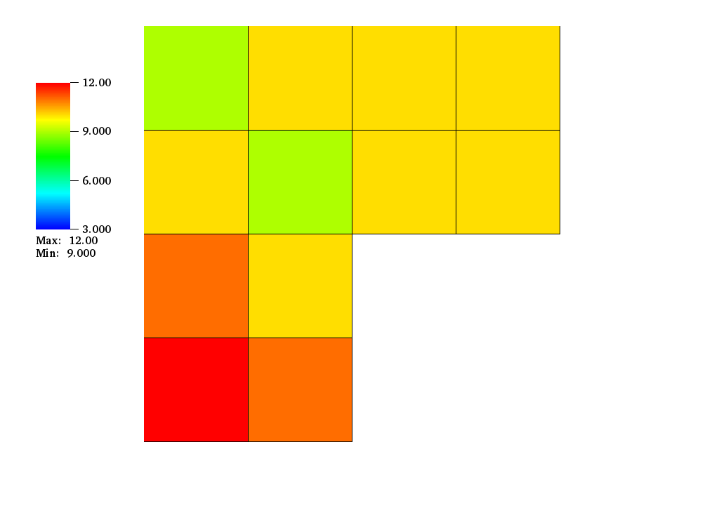
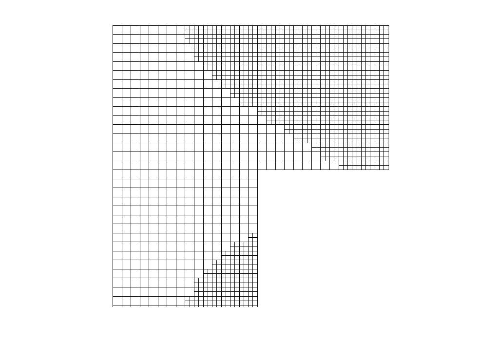
Figure 1: Example 1. Left: Final mesh after 11 $hp$-adaptive refinement steps, with color indicating the polynomial degrees. Right: Final mesh after 7 $h$-adaptive refinement steps. Both meshes have approximately the same number of degrees of freedom.

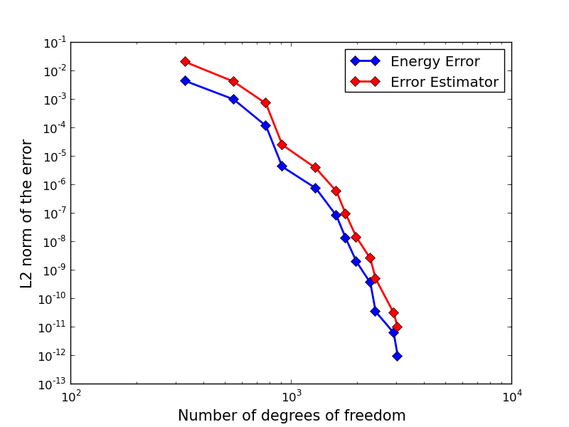
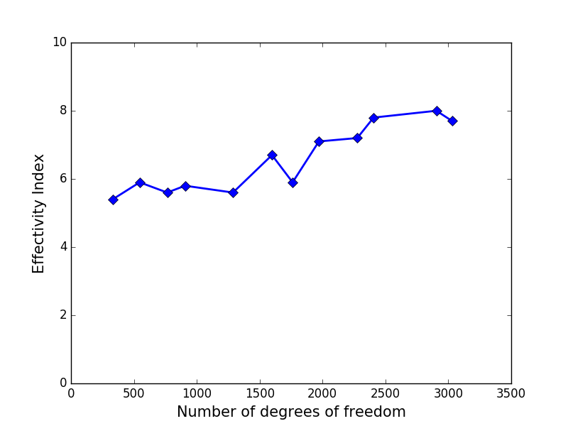
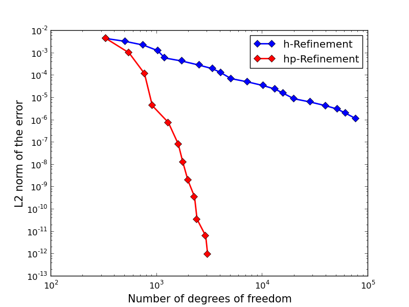
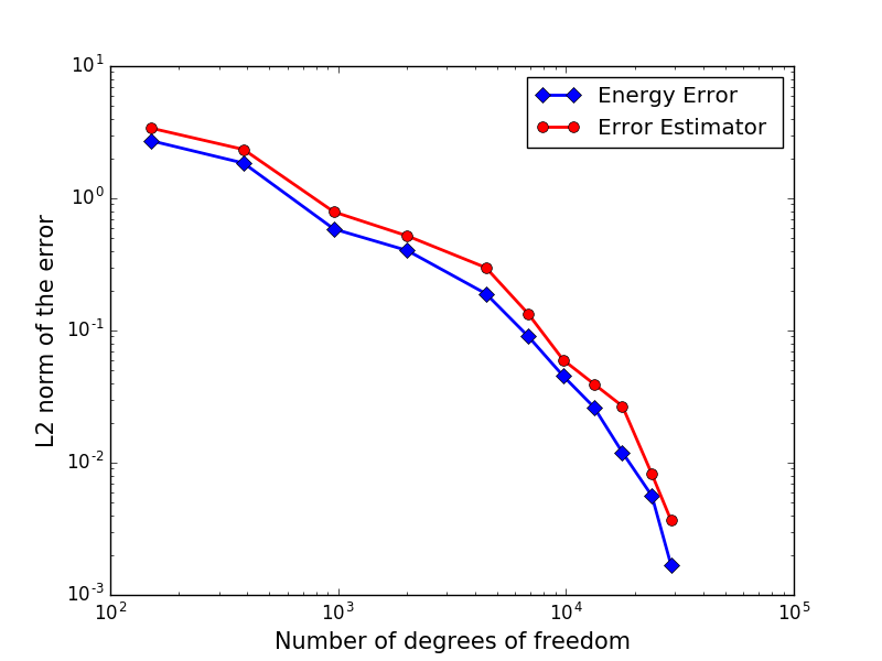
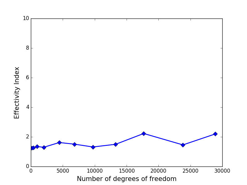
Fig. 1 shows meshes after a number of cycles if $hp$-refinement is allowed, or if we only do $h$-refinement. Unsurprisingly, and confirming expectations, given the smooth nature of the exact solution, the $hp$-adaptive strategy consistently chooses $p$-refinement. Fig. 2 presents the decay of the energy error and the a posteriori error estimator as a function of number of degrees of freedom. The graph both demonstrates the exponential convergence rate, and also that the $hp$-error estimator is a sharp upper bound for the energy error – validating this as an efficient and reliable a posteriori error estimator. We observe from the effectivity index graph in Fig. 2 that the $I_{\text{eff}}$ remains bounded in the range $5.4\leqslant I_{\text{eff}}\leqslant 8.1$.

The figure’s right panel also shows a comparison of errors for $h$- and $hp$-adaptive refinement strategies. This plot clearly shows the superiority of $hp$-AFEM over the $h$-AFEM.

Figure 2: Example 1. Left: Comparison of the energy error and the error estimator for an $hp$-adaptive computation. Center: Effectivity indices $I_{\text{eff}}$ for the same computation. Right: A comparison of the errors for this computation with the errors obtained through pure $h$-refinement.

6.2 Example 2

On the same $L$-shaped domain, we now choose right hand side and boundary values so that we reproduce the singular solution of [19], which reads in polar coordinates as

$$u(r,\varphi) =r^{\alpha}\left[\begin{matrix}\cos(\varphi)\psi^{{}^{\prime}}(\varphi)+(1+\alpha)\sin(\varphi)\psi(\varphi)\\ \sin(\varphi)\psi^{{}^{\prime}}(\varphi)-(1-\alpha)\cos(\varphi)\psi(\varphi)\end{matrix}\right],$$

$$\varrho(r,\varphi) =-r^{\alpha-1}\frac{(1+\alpha)^{2}\psi^{{}^{\prime}}(\varphi)+\psi^{{}^{\prime\prime\prime}}(\phi)}{1-\alpha},$$

where

$$\psi(\varphi)=\frac{\sin((1+\alpha)\varphi)\cos(\alpha\omega)}{1+\alpha}-\cos((1+\alpha)\varphi)\\ -\frac{\sin((1-\alpha)\varphi)\cos(\alpha\omega)}{1-\alpha}+\cos((1-\alpha)\varphi),$$

and $\omega=\frac{3\pi}{2}$. Here $\alpha$ is the smallest positive solution of $\sin(\alpha\omega)+\alpha\sin(\omega)=0$ and is $\alpha\approx 0.54448373678246$. We choose the same initial triangulation, but this time start with $\mathcal{Q}_{2}^{2}\times\mathcal{Q}_{1}$ elements on all cells. We use $\theta=0.85$.

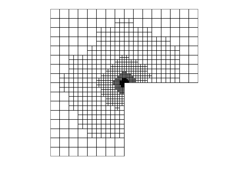
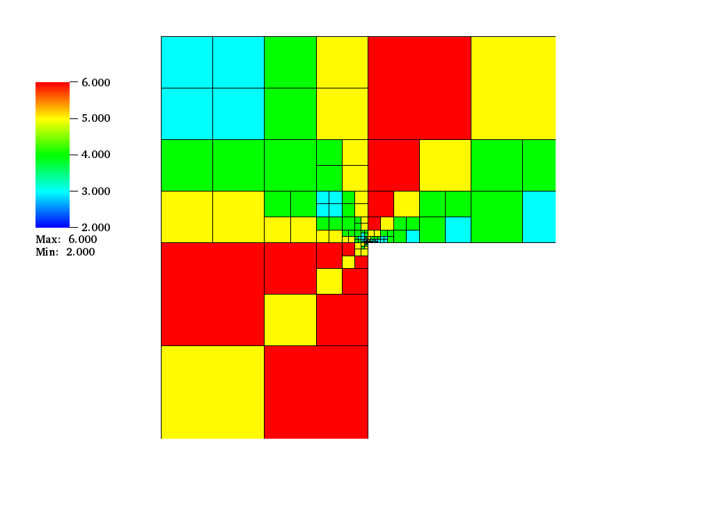
Fig. 3 again shows $hp$- and $h$-adaptively refined meshes generated by our error estimator. The corner singularity in the solution is apparent. A comparison of error and error estimator, efficiency indices, and a comparison between $hp$- and $h$-adaptively refinement strategies is shown in Fig. 4. In particular, the efficiency indices again remain bounded.

Figure 3: Example 2. Left: Final mesh after 10 $hp$-adaptive refinement steps, with color indicating the polynomial degrees. Right: Final mesh after 12 $h$-adaptive refinement steps. Both meshes have approximately the same number of degrees of freedom.

Figure 4: Example 2. Left: Comparison of the energy error and the error estimator for an $hp$-adaptive computation. Center: Effectivity indices $I_{\text{eff}}$ for the same computation. Right: A comparison of the errors for this computation with the errors obtained through pure $h$-refinement.

6.3 Example 3

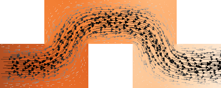
As our last example, we consider a less contrived flow field of a fluid moving through a pipe with a bend. The exact solution is here not known, but the solution on a very fine grid is shown in Fig. 5.

For this case, we prescribe homogeneous Dirichlet boundary condition on the sides of the pipe; for the inlet and outlet, we prescribe parabolic velocity boundary conditions. The adaptive algorithms uses $\theta=0.75$ and starts with 28 equally sized cells. The meshes generated by $h$-adaptive refinement are shown in Figure 5.

Figure 5: Example 3. Left: Pressure field and velocity vectors on a fine mesh. Right: The mesh after 12 $h$-adaptive refinement steps.

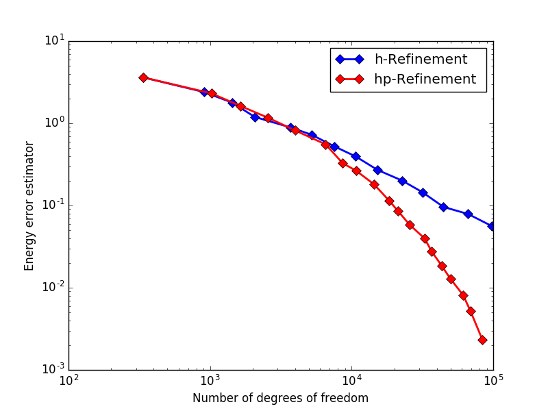
A comparison between the $h$- and $hp$-adaptively generated meshes in Fig.s 5 and 6 shows the expected pattern of h-refinement where the solution is not smooth, and $p$ refinement (if allowed) where the solution is smooth. Because the exact solution is not known, it is not possible to compare the exact errors for these two strategies; however, having established the quality of our error estimator in the previous example, we can compare how quickly the error estimates are reduced for both strategies, with results shown in Fig. 7 – clearly showing the superiority of $hp$ refinement.

Figure 6: Example 3. Mesh generated after 16 $hp$-adaptive steps, where the color bar indicates the polynomial degrees

Figure 7: Example 3. Comparison of the energy error estimator with $h$- and $hp$-adaptive mesh refinement.

7 Conclusion

In the spirit of previous work by Melenk on other equations (see [28, 29]), we have here introduced a residual-based a posteriori error estimator for the Stokes problem for continuous, $hp$-adaptive finite element methods (AFEM). In particular, we have introduced a family $\eta_{\alpha},\alpha\in[0,1]$ of residual based error estimators. We then proved upper and lower bounds for the estimators applied to the Stokes problems. We were inspired by Dörfler and Heuveline’s work [21] for one-dimensional problems and later work on higher space dimensions by Bürg [16], and introduced an $hp$-adaptive refinement algorithm for our application. In order to decide which refinement gives the best possible $hp$-refinement, in terms of the largest error reduction, we solve local patch problems in parallel for each individual cell. The numerical examples demonstrate the exponential convergence rate for $hp$-AFEM in comparison with $h$-AFEM. They also show the efficiency and reliability of the estimator with respect to the norm of the exact error.

8 Acknowledgements

This material is based upon work supported by the U.S. Department of Energy, Office of Science, under contract number DE-AC05-00OR22725. AG and WB’s work was supported by the National Science Foundation under award OCI-1148116 as part of the Software Infrastructure for Sustained Innovation (SI2) program. WB was also supported by the Computational Infrastructure in Geodynamics initiative (CIG), through the National Science Foundation under Awards No. EAR-0949446 and EAR-1550901, administered by The University of California – Davis.

References

• [1] M Ainsworth and J. T. Oden, A posteriori error estimation in finite element analysis, Comput. Methods. Appl. Mech. Eng., 142 (1997), pp. 1–88.
• [2] M. Ainsworth and B. Senior, An adaptive refinement strategy for hp-finite-element computations, Appl. Numer. Math., 26 (1998), pp. 165–178.
• [3] D. Arndt, W. Bangerth, D. Davydov, T. Heister, L. Heltai, M. Kronbichler, M. Maier, J.-P. Pelteret, B. Turcksin, and D. Wells, The deal.II library, version 8.5, Journal of Numerical Mathematics, 25 (2017), pp. 137–146.
• [4] D. N. Arnold, F. Brezzi, and M. Fortin, A stable finite element for the Stokes equations, Calcolo, 21 (1984), pp. 337–344.
• [5] I. Babuška, Error estimates for adaptive finite element computations, SIAM J. Math. Anal.J. Numer. Anal., 15(4) (1978), pp. 736–754.
• [6] I. Babuška and M. R. Dorr, Error estimates for the combined h- and p-versions of the finite element method, Numer. Math., 37(2) (1981), pp. 257–277.
• [7] I. Babuška and W. C. Rheinboldt, A posteriori error estimates for the finite element method, Int. J. Numer. Methods Eng., 12 (1978), pp. 1597–1615.
• [8]  , Adaptive approaches and reliability estimations in finite element analysis, Comput. Meth. Appl. Mech. Engrg., 17 (1979), pp. 519–540.
• [9] I. Babuška, B. Szabó, and I.N. Katz, The p-version of the finite element method, SIAM J. Numer. Anal., 18 (1981), pp. 515–545.
• [10] W. Bangerth, R. Hartmann, and G. Kanschat, deal.II a general purpose object oriented finite element library, ACM Trans. Math. Software, 33(4) (2007), pp. 24/1–24/27.
• [11] W. Bangerth and O. Kayser-Herold, Data structures and requirements for hp𝑝hp finite element software, ACM Trans. Math. Softw., 36 (2009), pp. 4/1–4/31.
• [12] W. Bangerth and R. Rannacher, Adaptive Finite Element Methods for Differential Equations, Birkhäuser Verlag, 2003.
• [13] C. Bernardi, R. G. Owens, and J. Valenciano, An error indicator for mortar element solution to the Stokes problem, SIAM J. Numer. Anal., 21 (2001), pp. 857–886.
• [14] F. Brezzi, On the Existence, Uniqueness, and Approximation of Saddle-Point Problems Arising from Lagrangian Multipliers, RAIRO Anal. Num., 8 (1974), pp. 129–151.
• [15] M. Bürg, A residual-based a posteriori error estimator for the hp-finite element method for Maxwell’s equations, Appl. Numer. Math., 62 (2012), pp. 922–940.
• [16] M. Bürg and W. Dörfler, Convergence of an adaptive hp finite element strategy in higher space-dimensions, Appl. Numer. Math., 61 (2011), pp. 1132–1146.
• [17] Ph. Clément, Approximation by Finite Element Functions Using Local Regularization, RAIRO Anal. Num, 9 (1975), pp. 77–84.
• [18] M. Costabel, M. Dauge, and C. Schwab, Exponential convergence of hp-FEM for maxwell’s equations with weighted regularization in polygonal domains, M3AS, 15(4) (2005), pp. 575–622.
• [19] M. Dauge, Stationary Stokes and Navier-Stokes systems on two- or three-dimensional domains with corners, part i: Linearized equations, SIAM J. Math. Anal., 20 (1989), pp. 74–97.
• [20] L. Demkowicz, W. Rachowicz, and Ph. Devloo, A fully automatic hp-adaptivity, J. Sci. Comput., 17 (2002), pp. 127–155.
• [21] W. Dörfler and V. Heuveline, Convergence of an adaptive hp finite element strategy in one space dimension, Appl. Numer. Math., 57 (2007), pp. 1108–1124.
• [22] T. Eibner and J.M. Melenk, An adaptive strategy for hp-FEM based on testing for analyticity, Comput. Mech., 39 (2007.), pp. 575–595.
• [23] A. Ern and J. L. Guermond, Theory and Practice of Finite Elements, 2013.
• [24] V. Girault and P. A. Raviart, Finite Element Approximation of the Navier-Stokes Equations. Series in Computational Mathematics., 1986.
• [25] V. Heuveline and R. Rannacher, Duality-based adaptivity in the hp-finite element method, J. Numer. Math., 11(2) (2003), pp. 95–113.
• [26] P. Houston, D. K. Schötzau, and T. P. Wihler, hp𝑝hp-adaptive Discontinuous Galerkin finite element methods for the Stokes problem, in European Congress on Computational Methods in Applied Sciences and Engineering (ECCOMAS), 2004.
• [27] J.M. Melenk and C. Schwab, hp-FEM for reaction-diffusion equations, robust exponential convergence, SIAM J. Numer. Anal., 35 (1998.), pp. 1520–1557.
• [28] J. M. Melenk, hp-interpolation of nonsmooth functions and an application to hp-a posteriori error estimation, SIAM J. Numer. Anal., 43 (2005), pp. 127–155.
• [29] J. M. Melenk and B. I. Wohlmuth, On residual-based a posteriori error estimation in hp-FEM, Adv. in Comput. Math., 15 (2001), pp. 311–331.
• [30] W. Rachowicz, J.T. Oden, and L. Demkowicz, Toward a universal h-p adaptive finite element strategy part 3. design of h-p meshes, Comput. Meth. Appl. Mech. Engrg., 77(1-2) (1989), pp. 181–212.
• [31] D. Schötzau and C. Schwab, Exponential convergence in a Galerkin least squares hp-FEM for Stokes flow, IMA J. Numer. Anal., 21 (2001), pp. 53–80.
• [32] CH. Schwab, p- and hp-Finite Element Methods, 1998.
• [33] L. R. Scott and S. Zhang, Finite Element Interpolation of Nonsmooth Functions Satisfying Boundary Conditions, Math. Comput., 54 (1990), pp. 483–493.
• [34] B. Szabó and I. Babuška, Finite Element Analysis, 1991.
• [35] R. Verfürth, A posteriori error estimator for the Stokes equations, Numer. Math., 55 (1989), pp. 309–325.
• [36] R. Verfürth, A review of a posteriori error estimation and adaptive mesh-refinement techniques, Wiley, Chichester, 1996.
• [37] T. P. Wihler, An hp-adaptive strategy based on continuous sobolev embeddings, J. Comput. Appl. Math, 235 (2011), pp. 2731–2739.