Numerical approximation of a mechanochemical
interface
model for skin appendage††thanks: This work was partially supported by grants
from the Swiss National Science Foundation (FNSNF, grants 31003A_140785
and SINERGIA CRSII3_132430), by the SystemsX.ch initiative (project Epi-PhysX);
and by the Engineering and Physical Sciences Research Council (EPSRC, research grant EP/R00207X/1).
Abstract
We introduce a model for the mass transfer of molecular activators and inhibitors in two media separated by an interface, and study its interaction with the deformations exhibited by the two-layer skin tissue where they occur. The mathematical model results in a system of nonlinear advection-diffusion-reaction equations including cross-diffusion, and coupled with an interface elasticity problem. We propose a Galerkin method for the discretisation of the set of governing equations, involving also a suitable Newton linearisation, partitioned techniques, non-overlapping Schwarz alternating schemes, and high-order adaptive time stepping algorithms. The experimental accuracy and robustness of the proposed partitioned numerical methods is assessed, and some illustrating tests in 2D and 3D are provided to exemplify the coupling effects between the mechanical properties and the advection-diffusion-reaction interactions involving the two separate layers.
Key words: Elasticity-diffusion problem; Interface coupling; Pattern formation; Skin appendage modelling; Finite element methods; Adaptive time stepping.
Mathematics subject classifications (2000): 92C15, 35Q92, 65M60, 74S05, 35K57, 74A50.
1 Introduction and modelling considerations
Reliable modelling of mechanochemical properties of composite materials is of key importance in a variety of engineering, material science and life science applications. These include tissue engineering, wound healing manipulation, bone fracture repair, design of photovoltaic devices, polymer adhesion, and many others. Of special interest to us are the two-way interactions between, on one hand, biological tissue deformation and, on the other hand, migration and proliferation of certain cell types during organismal development.
One application of such a general model is the study of the vertebrate skin appendage development and evolution, especially their diversity of forms (such as hairs, spines, feathers, and scales; [25, 36, 37, 44]), and spatial organisations. Note that we have recently shown that all skin appendages are homologous structures developing from an anatomical placode and associated signalling molecules [17].
Turing proposed in his seminal work [59] that pattern formation in biological systems could be explained by a system of diffusion and interacting chemicals that he called ’morphogens’. Many subsequent studies [33, 44, 52, 50] investigated biological patterning in the framework of such purely chemical reaction-diffusion models. However, as already suggested by Turing [59], mechanical aspects might also be relevant to biological patterning processes. During the last decade, biological experiments have clearly indicated that not only chemical (pattern of morphogen concentrations), but also mechanical (stresses and strains), parameters are key to skin development [1, 3, 25, 42, 58] and are synchronised during embryonic development [40].
Although the full detailed underlying mechanisms are still incompletely understood, authors have attempted to integrate both chemical and mechanical parameters in their mathematical models of skin patterning [41, 43]. The various proposed mechanochemical models differ by the nature of the interactions between morphogen concentration and mechanics. For instance, while in [39, 56] mechanical responses are directly triggered by chemical signalling, other models [38, 39] propose that migration of cells directly generate local forces on the tissue. Such interactions between cells and morphogens can be complemented with chemical and mechanical exchanges between the two layers (dermis and epidermis) that constitutes the skin [15, 51]. In one example [6], a three-chemical species model of limb bud development integrates growth velocity of the tissue normal to the limb surface and that directly depends on the local concentration of fibroblast growth factor. Other models consider the tissue growth as a liquid displacement [13], or aggregation of cells is the result of a chemical pre-pattern.
Here we focus on the computational modelling of mechanochemical interactions (inspired by [15] and [51]) based on simple reaction-diffusion systems governing the relations between, on one hand, the concentration of morphogenic proteins and cells densities and, on the other hand, mechanical stresses and strains. The mathematical description proposed in these two references is sufficiently general to be applied to multiple biological contexts (e.g., angiogenesis, fingerprint formation, cartilage condensation [41]), justifying the numerical algorithm presented here. Experimental evidence shows that the skin short-term and low-amplitude response to mechanical stimuli is that of an elastic solid [16]. We therefore assume that the two-layer domain of the skin (dermis and epidermis) can deform according to its inherent mechanical response, and that it is affected isotropically via an internal force that depends on the signalling factors. In addition, given the long spatio-temporal scale of the organismal developmental process, short-term fluctuations and inertial effects can probably be safely discarded to simplify the mathematical model [38]. We therefore adopt the two following fundamental assumptions: (i) the equilibrium of forces in the system is established by a quasi-static balance of linear momentum, and (ii) chemical species, governed by an advection-diffusion reaction (ADR) system, affect the medium deformation (through coupling functions). The chemical species’ dynamics represents the spatio-temporal evolution of two morphogenic proteins and/or of cells that trigger and control the internal forces affecting the momentum balance. In turn, cell motion induces local and global traction forces on the elastic body, leading to substrate deformations [42]. We point out that cell motility depends on different factors that include kineses (increase in motile activity without any directional component), taxes (directed motion up or down a gradient), and guidances (motion directed by substratum cues, also called contact guidance) [39] that can also act locally or globally. Although long-range effects can be implemented through high-order spatial derivatives (appearing in the ADR or force conservation equations), we will here incorporate only short-range effects because our focus is on the numerical and algorithmic aspects of interface problems (such as the dermis-epidermis interactions in the skin).
As suggested elsewhere [15], here we distinguish between the two very different cellular dynamics of the dermis and the epidermis. Whereas we adopted a general logistic growth mitotic rate and non-negligible short range cell diffusion [40] in the dermis, we account for a zero production rate of cells and very small diffusivities in the equations governing epidermal variables [1, 51]. This difference of treatment in the two tissues is justified by their respective structures: cells in epidermal tissue form sheets of adjoined interacting cells, while mesenchymal cells in the dermis are more mobile and separated by substantial extracellular matrix. However, as epidermal cells are not completely attached to each other and can rearrange topologically [1], we assume in both dermis and epidermis that all diagonal terms in the diffusivity matrices are strictly positive.
Regarding the interface problem between dermis and epidermis, we considered multiple methods for numerical approximation of linear elasticity using mixed finite elements: parallel and sequential Schwarz iterations using various interface conditions based on boundary element-finite couplings [23], -mortar [9], Nitsche [8], multiscale settings [11], or matching interface algorithms [62]. We finally chose a Schwarz iteration method with domain decomposition where the coupled set of mechanochemical equations is solved separately on each side of the interface, imposing mixed-type (Robin) boundary conditions, i.e., both fluxes and density values are equal in both tissues at their interface. A rich body of literature deals with choosing the weighting coefficients on the Robin interface conditions in order to optimise the convergence of the alternating Schwarz algorithms under different scenarios (see e.g. [12, 21, 26, 55] and references therein). As the optimal weighting scheme tends to be problem-dependent and might change substantially for diffusion, elasticity, or fluid-oriented problems, we will only describe general schemes and mention which specific weighting best suits the problems we investigate here.
Here, we define a family of finite element methods for the semi-discretisation of the problem, where the classical MINI-element [5] is used for the approximation of both displacement and pressure on each subdomain, whereas piecewise linear and continuous elements are used to discretise the vector of species concentration. Concerning the fully-discrete (spatial and time discretisation) scheme for the model problem, we apply an adaptive time-stepping strategy based on diagonally-implicit Runge-Kutta methods. This so-called TR-BDF2 method was introduced in the context of electronic circuit simulation [7] (see also [10, 29, 19] for further details) and has the advantage of using the same Newton iteration matrix to solve different temporal stages within a time step, a particularly interesting feature when addressing large systems of ODEs. The step size adaptivity exploits classical automatic control techniques used in the integration of so-called stiff systems [27, 28], i.e., problems that tend to be numerically unstable.
This article is organised in the following manner. The remainder of this section contains preliminary notation and generalities to be used throughout the paper. Section 2 provides a detailed description of the differential equations constituting the model problem, with special emphasis on the coupling occurring at the interface. In Section 3, we introduce the Galerkin method, we present the adaptive time discretisation, and we specify algorithmic considerations. Section 4 contains a collection of computational tests focusing on the accuracy of the numerical schemes and on the suitability of the model equations to represent mechanochemical problems. We close with a summary and discuss potential extensions of the model in Section 5.
Throughout the paper, we let , denote a deformable body with polyhedral boundary , and denote by the outward unit normal vector on . Moreover, given a generic domain , , for two vectorial functions will denote their inner product as , whereas if is a dimensional surface then their pairing will be written as . In addition, by we will denote the space of polynomial functions of degree defined on the domain , and stands for the identity matrix in . Finally, we will employ to denote a generic null vector or the zero operator.
2 Set of governing equations
Linear elastic solids.
We assume that the domain is disjointly divided into two connected subdomains (with different material properties) denoted by and , respectively, whose intersection constitutes the interface between the regions and is denoted . On we define a part of the boundary related to the exposed surface, denoted as (see Figure 2.1).
This heterogeneity of the skin (corresponding to the presence of an homogeneous dermis and an homogeneous epidermis, occupied by and , respectively) is accounted for by the spatially-dependent (but locally constant) Lamé coefficients
We also suppose that the two-layered elastic medium is nearly incompressible, so, in view of avoiding the well-known phenomenon of volumetric locking (inability of some discrete spaces to approximate the true displacement while satisfying incompressibility, see e.g. [9]), a mixed formulation is adopted in terms of displacements and the pressure , with D,E (although the interpretation of as pressure holds exclusively in the incompressibility limit where takes on quite large values). For all , and given a body force (whose specific form depends on the vector ; see equation (2.5) below) applied on each domain, we resolve the displacement / pressure pair on each subdomain, satisfying spring conditions at the surface boundary (Robin conditions), having clamped boundaries elsewhere, and assuming an adhesion condition at the interface (matching displacements and preservation of traction forces imply continuity of the medium across ). Then the global linear Navier-Lamé problem adopts the form
| (2.1) | |||||
where is the tensor of infinitesimal strains (symmetric gradient of displacement), is the Cauchy stress tensor, and is the Robin coefficient. The extension to non-homogeneous displacement conditions () can be handled in a standard way by adding suitable liftings on the data. Below, we use the asterisk superscript D,E to denote quantities related to each subdomain, and we adopt the convention that the unit normal vector on the interface is pointing from to .
We stress that modelling the development of soft tissue and cells, in terms of mechanical dynamic behaviour is still an active area of research [2, 61]. Biological tissues, depending on the nature of the constituent cells, present a large variability in their elastic properties (including viscous, nonlinear, or nonlocal effects) which can change substantially through spatio-temporal scales [35, 45, 61]. Some recent analyses were based on nonlinear St. Venant-Kirchhoff descriptions [35], including viscoelastic terms [2, 39, 57, 59], and even fluid dynamics, as mentioned in [61]. A general consensus on how to represent mechanical properties of the skin tissue under morphogenesis is not yet available. Hence, our description will be restricted to classical linear elastic materials because it accurately represents small tissue deformations manifested during the first stage of skin appendage formation.
Advection-diffusion-reaction equations on an underlying deforming medium.
Let us focus on the spatio-temporal interaction of the densities of species . We assume that all constituent species are equi-present at each spatial point (i.e., they are spatially continuous), so applying the Reynolds transport theorem to their mass conservation (assuming zero-flux boundary conditions at the surface and continuity of fluxes and densities at the interface) leads to the system
| (2.2) | |||||
Here is a (not necessarily diagonal, but positive definite) tensor of self- and cross-diffusion rates, is a vectorial function containing the reaction kinetics of the system and representing the production and degradation of species concentration on each subdomain ; and the term encodes an additional coupling contribution (detailed in equation (2.5) below). The system is endowed with adequate initial conditions for , and the general form (2.2) accommodates either dimensional or dimensionless descriptions.
Here,we focus on two levels of model complexity. Firstly, we define a simple two-variable activator-inhibitor model with quadratic reaction terms due to Gierer-Meinhardt (cf. [24]):
| (2.3) |
where is the short-range autocatalytic substance and is the long-range antagonist; and the ’s are positive model parameters.
Second, we introduce a more general model of skin appendages development were is the cell density, is the density of the extracellular matrix, and are the concentrations of two morphogen signalling chemical compounds. All quantities are assumed to diffuse, so none of the diagonal terms in is zero (nevertheless, self-diffusion for cell concentration in the epidermis and the matrix density in the two tissues, will be very small in comparison to the other values in the diagonal of ), and we discard higher order terms (derivative with order higher than two) representing haptotaxis and non-local effects in the cell migration fluxes. The reactions consist in a logistic relation for the mitotic rate, a zero rate of matrix material secretion, and the production, as well as degradation, of morphogens:
| (2.4) |
where is the maximum cell density, and ’s are positive model constants. The specifications in (2.4) have been adapted from the skin pattern formation model proposed in [15]. Similar models can be found in the context of cell migration, angiogenesis, follicle differentiation, or mesenchymal morphogenesis (see e.g. [1, 34, 37, 43, 60]).
Coupling mechanisms.
Extensive experimental evidence indicates that both biochemical and mechanical processes work in concert during pattern formation (see for instance [1, 2, 25, 30, 35, 53]). In the specific context of skin appendage formation, signalling pathways control cell movements that eventually lead to mechanical tissue deformation due to cell aggregation [1, 25, 53]. These interactions can be represented by diverse local or non-local processes including advection, cytoskeleton regulation, chemical gradients, active stress, strain dependent diffusivity, and many others [40, 38]. In the present model we opt for including only local variations of the ADR and mechanical variables. This simplification rules out some phenomena such as inter-cellular force transmission through cytoskeleton, nonlinear interactions (e.g., cells sensing, through filopodia, long-range variations), or anisotropy effects, which can be of special importance in some biological contexts [15, 34]. Nonetheless, as suggested in [38], local models such as the one we use here, may suffice to reproduce accurately a variety of mechanical processes without the need for additional constitutive relations.
The PDE-based model (2.1)-(2.2) (written in Eulerian form and solving for displacements, solid pressure, and molecular variables) assumes that changes in the chemical concentrations do not affect the mechanical properties of the solid, nor the Lamé constants; the species only act as forcing terms on the momentum balance, i.e., the intensity of the deformation will depend locally on the gradient of the species concentrations. Conversely, we here suppose that the body deformation affects the species dynamics by means of advection and through the term on the right-hand side in (2.2), carrying local information about the medium dilation. Therefore, we set
| (2.5) |
where are model parameters. Note that the form of is equivalent to considering a stress component depending on the concentrations of some , that is , where is an effective elastic stress. Similar coupling conditions can be found in [22, 31, 49].
2.1 Weak formulation for the multidomain problem
Multiplying (2.1)-(2.2) by suitable test functions, integrating by parts over each region , and exploiting the boundary and interface conditions, we arrive at the following primal-mixed variational problem associated to the elasticity-ADR problem: For , find such that
| (2.6) | |||||
where is the coefficient associated to the Robin boundary condition at the surface, and the specific boundary treatment implies that adequate functional spaces are
Linear and nonlinear forms (lowercase and uppercase, respectively) involved in (2.6) are defined as
The unique solvability of (2.6) has not yet been addressed in the literature, however related results concerning the coupling of linearised mechanics and reaction-diffusion systems have been recently addressed in the context of cardiac and plant cell biomechanics [4, 46].
Treating the interface: a non-overlapping continuous Schwarz method.
As mentioned previously, the treatment of the interface (here, between the epidermis and dermis) is an important issue for interacting media problems and this paragraph will focus on its realisation. Regarding the geometric separation between the problems defined on each side of the interface, we remark that (2.6) is valid in particular if we consider a solution globally defined in . Nevertheless, in the discrete case we aim at solving two separate problems on each subdomain and therefore we require to impose jump conditions in an adequate manner. We adopt a non-overlapping Schwarz iteration based on Robin-Robin type interface conditions for the ADR system
| (2.7) |
where denotes the Robin transmission operator, and are nonnegative acceleration constants satisfying (see, for instance [32] and [18, 47]). On the other hand, the adhesion interface condition featured by the elasticity problem is incorporated through the following relation
| (2.8) |
where is a transmission operator associated to the elasticity problem, and is another acceleration constant. The classical iterative Schwarz algorithm (still continuous and still nonlinear) then reads: For and for , find such that
| (2.9) | |||||
where
and the superscript D,E denotes quantities in the subdomain opposite to . Here we have dropped the explicit time-dependence whenever clear from the context.
3 A finite element method and its splitting scheme
In this section we detail a Rothe-type strategy employed to numerically solve the set of governing equations (2.1)-(2.2). We first apply a discretisation in space written as a primal-mixed Galerkin formulation, which we later combine with fixed-point schemes and a Schwarz iterative algorithm decoupling the problem into four main blocks corresponding to each side of the interface, and to the elasticity and ADR equations. Then we discuss the time discretisation based on an adaptive scheme and operator splitting.
3.1 Nonlinear, partitioned Galerkin formulation
Let us denote by a shape-regular simplicial partition of by triangles (for , or tetrahedra for ) of diameter and define the global meshsize as . For clarity of the presentation, we assume that the two meshes (associated with each subdomain) match at the interface. We will seek the approximation of , in the finite dimensional product space
| (3.1) |
to be made precise below. Then, the semidiscrete Galerkin scheme associated to the Schwarz alternating algorithm (2.9) and a fixed-point decoupling of elasticity and ADR subproblems can be recast in the following partitioned form, iterated until convergence: For a given , and given , find the next iteration from the sequential system
| (3.2) | |||
| (3.3) | |||
| (3.4) | |||
| (3.5) |
Note that the order in which these blocks are solved is arbitrary. We also note that the blocks (3.2),(3.5) still constitute nonlinear problems, that we solve through inner Newton iterations. Alternatively, one can commute the domain decomposition method and the nonlinear solvers, in such a way that the nonlinearly coupled set of equations can be solved monolithically on each subdomain. Further details on the choice we adopt here, are provided in Algorithm 1, below. Finally we remark that the sequential steps (3.2)-(3.5) can be regarded as a block Gauss-Seidel iteration applied to the fully monolithic differential-algebraic system.
For the discretisation of the elasticity equations in mixed form, we require the discrete spaces in (3.1) to be inf-sup stable. In our implementation we choose the so-called MINI elements [5], characterised by
where is the space of cubic bubble functions defined locally on an element ; and we employ the space of conforming Lagrangian finite elements for the approximation of the species concentrations
The discretisation (3.2)-(3.5) leads to the following system of equations
| (3.6) | ||||
| (3.7) | ||||
where the superscript may be replaced by the appropriate index associated to the Schwarz algorithm. We readily observe that only (3.6) is a nonlinear ODE system, whereas the matrix form of the elasticity sub-problem consists of a linear system. The subscript in emphasises that the matrix is directly dependent on displacements.
3.2 Adaptive timestep scheme
The family of fully-discrete methods that we use here is based on adaptive, embedded Runge-Kutta schemes of order 2 and 3 (RK23). For a generic ODE system , we recall that the main step in the classical RK23 scheme reads
with stages, and where the two approximations are of order and , respectively. As in classical embedded RK methods, here the coefficients coincide in both approximations; however the coefficients differ in order to attain the expected convergence orders (in general one chooses , cf. [27]). Even when the stability properties of the two schemes do not match, embedded RK methods provide a rather non-expensive estimator for the local error (of the less accurate solution) which is then directly used in the control of the timestep [27, 28]. The specific description of the controller used here is presented in Algorithm 2, below.
| 0 | 0 | 0 | 0 |
|---|---|---|---|
| 0 | |||
| 1 | |||
The RK23 scheme is used together with the TR-BDF2 method (see [7]), which is a particular class of Diagonally Implicit Runge-Kutta (DIRK) methods (that is, for , and at least one ) [27]. The scheme is characterised by the following Butcher’s tableau reported in Table 3.1, where , , and .
As established in [29], the A-stability, the stiffly accuracy (, for ), as well as the strong S-stability of the method are guaranteed by the coefficients used in Table 3.1. An appealing advantage of this scheme is that, for each step, only two implicit stages are required (where one can reuse the same Newton iteration matrix) while one stage is explicit. In this regard, the method is closely related to singly DIRK (SDIRK) methods (where all diagonal coefficients are equal and the first stage is explicit) [29]. In addition, TR-BDF2 falls in the class of First-Same-As-Last (FSAL) RK schemes, i.e. methods where the current explicit stage coincides with the last stage of the previous step, therefore decreasing the overall computational cost.
Based on Table 3.1, and considering (where we have removed the Schwarz index whenever clear from the context), we can recast the intermediate stages as
These problems should be solved through Newton iterations before moving to the next timestep. Alternatively, and as suggested in [28], one can apply the change of variables and rewrite the problem accordingly. Doing so results in decreasing round-off errors and serves in reducing the cost to compute . We follow this approach and modify the superscripts , and , to obtain the following full discretisation of the ODE system:
with
This nonlinear system is solved by means of Newton steps as follows
where
We finally point out that an additional reduction of computational cost occurs due to the fact that the local error can be accessed by the simple relation
avoiding the explicit storage and computation of .
3.3 Algorithmic details
Overall solution algorithm. The global numerical scheme to solve the mechanochemical model is summarised in Alg. 1. After assigning suitable initial conditions , , , projected to the corresponding finite element spaces, we use the non-overlapping Schwarz method (3.2)-(3.5) to produce a solution until time . Two important points stand out from this master algorithm. First, only the ADR equations are solved through the embedded RK method within the TR-BDF2 method (see Alg. 1, Line 8, detailed in Alg. 2), whereas the elasticity subproblem is solved by an implicit method (cf. Line 11 in Alg. 1). Furthermore, the velocity in the advection term is approximated from the solid displacement using a backward Euler scheme (cf. Alg. 1, Line 10 and 12). Second, the computation performed in Alg. 1, Line 5 and 18, represents an alternative way of performing the explicit first stage of the RK scheme [29]. Such a rescaling must be executed at each modification of the timestep, so that one starts with an adequate value for when entering Line 8 of Alg. 1. An additional benefit of the rescaling is that it improves the stability of the overall stiff problem, and at the same time avoids unnecessary function evaluations.
Adaptive Runge-Kutta method. The RK procedure is detailed in Alg. 2 and it features a similar structure as the ODE solver ode23tb in MATLAB. Again, we highlight two major components: the one-step RK resolution and the adaptive setting of the timesteps. Line 2 in Alg. 2 represents stage 2 of the RK method, i.e., the first implicit stage (S1). As the scheme is implicit, we initialise the tangent system associated to the Newton iteration. These matrices will actually be assembled only if the Boolean mjcontrol is true, and this switch is described in Alg. 4, below. Should mjcontrol be false, the mass-Jacobian blocks are evaluated at each Newton step (see Alg. 2, specifically Line 8). We also stress that the initial guess for the rescaled derivative can be simply taken as , since extrapolating the derivative of the interpolant from the previous step does not improve accuracy nor efficiency. Next, when updating the solutions we also change the Robin transmission conditions so that the Schwarz algorithm is performed at the same time (see Line 14 in Alg. 2). In order to retrieve and , a second Newton step is necessary within the implicit stage (S2), the particularity of which is the evaluation of the initial guess , by extrapolation of the derivatives of the cubic Hermite interpolant from to [29].
The algorithm also focuses on the automatic determination of each timestep, in view of the stability of the time integration of stiff problems. The process is designed to reject the overall step if one of the two implicit stages fails or if the local error is too large. The potential rejection at an implicit stage is monitored by the Boolean variables rejectS1 and rejectS2, which are switched on according to the value of the residual in the Newton iteration described in Alg. 3. How the value is actually computed may affect the performance of the algorithm (see e.g. [54]). For a generic residual vector of length , here we adopt the rescaled maximum norm
where is the local maximum of the solution vector at the -th Newton step, and it is reinitialised as , where . This process is summarised in Line 1 from Alg. 2.
We recall (see Line 1 of Alg. 3) that the residual in the Newton step is simply the norm of the current increment . The loop can break under different cases. For instance, if the residual is smaller than a given threshold, then Line 2 terminates the step. Otherwise, the linear convergence of the overall scheme (see e.g. [28]) implies that one can evaluate the iteration error using the residual together with the inequality , with . This experimental rate is reset to zero at each mass-stiffness assembly so that it depends on the Newton iteration matrix [48]. The rate is then estimated using (see Line 20) with two successive iterations and the current error. We consider that the algorithm has converged if the error is smaller than times a fixed tolerance. A given stage is therefore rejected if at least one of the following situations occurs: (a) the convergence rate is larger than 1 (cf. Line 16); (b) the maximum number of iterations is reached (cf. [28] and Line 23); and (c) For any , we have (cf. Line 26). Point (c) represents a rough estimate of the iteration error expected after iterations.
Should a stage be rejected, one moves to Line 25 in Alg. 2 and reduces the timestep by a factor (independently of the mass matrix assembly). Then, Line 31 checks whether both mass and Jacobian matrices have been updated. Finally, Line 36 verifies that the local error estimation remains below a prescribed tolerance. Based on the estimators for the scaled derivatives we proceed to compute the local asymptotic error as a result from the linear system stated in Line 42 of Alg. 2. This step is necessary as the boundedness of the raw estimator is not always guaranteed [28].
Next, we select the maximum error between these two estimators as an approximation of the timestep error. In contrast with [28], we do not observe here the so-called hump phenomenon intrinsic to automatic step methods, so we do not require an additional correction step. We only update the timestep in an automatic fashion (thanks to the sequence of rejection procedures), capturing correctly the dynamics of the integrated system. When all errors are lower than the corresponding tolerance, the timestep is accepted and the interface elasticity problem is solved in Line 11 from Alg. 1. We stress that the algorithm will stop if .
Alg. 4 permits to control the mass-stiffness assembly. This procedure consists of a number of controllers, including the aforementioned mjcontrol (see a list in Table 3.2). The state modification of these variables depends on step-size revaluation, which itself depends on the rejected stage of the RK method. Notice that Mcurrent and Jcurrent control whether the mass and Jacobian matrices are evaluated at each new timestep (if this timestep is rejected at least once). For models such as (2.2), the label Mcurrent is always true. However if we want to solve the interface problem using e.g. a level-set approach, then the mass matrix needs to be recomputed and the controller can be exploited.
| mjcontrol | Switch to reuse Newton iteration matrices over two implicit stages |
| needNewM | Need to evaluate mass matrix |
| needNewJ | Need to evaluate Jacobian matrix |
| needNewMJ | Need to evaluate mass-Jacobian matrix |
| Mcurrent | Appropriate mass matrix for the current timestep |
| Jcurrent | Appropriate Jacobian matrix for the current timestep |
4 Numerical tests
This section contains a set of examples assessing the experimental spatio-temporal convergence of our primal-mixed method, and also illustrates its use in two mechanochemical interface problems. The implementation is carried out with the open-source finite element library FreeFem++ [20], and all sparse linear systems are solved with distributed direct methods (MUMPS and UMFPACK).
| , , , , , , , |
| , , , , , , , , , |
| , , , e5, , , , e5, |
Example 1: Experimental accuracy against manufactured solutions.
Let us consider a rectangular domain divided into the dermis and epidermis subdomains. The initial position of the interface is characterised by the segment , and the external surface is . The main goal of our first series of tests is to analyse the convergence of the spatial discretisation. We therefore focus on a stationary problem where no advection occurs in the morphogen model. We construct smooth exact solutions, defined as follows:
| (4.1) |
and set , , , , and . The functions in (4.1) are used to construct the Dirichlet datum for the displacements on as well as the flux conditions imposed on the morphogens at the boundary . Suitable non-homogeneous forcing terms are also set using these closed-form solutions. We choose the two-species Gierer-Meinhardt reaction model (2.3), and adopt the coupling terms as in (2.5). Model parameters are chosen as in Table 4.1.
| Space convergence | ||||||||||
| DoF | ||||||||||
| 48 | 0.5207 | 5.6275 | – | 3.5698 | – | 1175.8 | – | 2.2114 | – | |
| 108 | 0.2828 | 4.1858 | 0.5794 | 2.6495 | 0.4886 | 444.12 | 1.9061 | 1.2433 | 0.9437 | |
| 280 | 0.1736 | 2.6223 | 0.7956 | 1.8701 | 0.7133 | 129.18 | 2.1008 | 0.6340 | 1.3790 | |
| 900 | 0.0889 | 1.4380 | 0.9447 | 0.9974 | 0.9398 | 37.750 | 1.9344 | 0.2178 | 1.5973 | |
| 3264 | 0.0432 | 0.7485 | 0.9844 | 0.4852 | 0.9978 | 11.335 | 1.8138 | 0.0801 | 1.3849 | |
| 12276 | 0.0218 | 0.3829 | 0.9890 | 0.2480 | 0.9788 | 3.6282 | 1.6805 | 0.0409 | 0.9624 | |
| 47320 | 0.0110 | 0.1970 | 0.9695 | 0.1326 | 0.9217 | 1.4185 | 1.3701 | 0.0252 | 0.9748 | |
| 186276 | 0.0055 | 0.1065 | 0.9928 | 0.0684 | 0.9605 | 0.7001 | 0.9599 | 0.0141 | 0.9635 | |
| DoF | Iter | |||||||||
| 48 | 0.5207 | 0.0605 | – | 1.2176 | – | 0.0423 | – | 0.5038 | – | 4 |
| 108 | 0.2828 | 0.0255 | 1.6925 | 0.6149 | 1.3372 | 0.0192 | 1.2900 | 0.3408 | 0.6409 | 4 |
| 280 | 0.1736 | 0.0081 | 1.9584 | 0.2545 | 1.5009 | 0.0093 | 1.4921 | 0.2226 | 0.8723 | 4 |
| 900 | 0.0889 | 0.0024 | 1.9235 | 0.1201 | 1.1808 | 0.0029 | 1.7335 | 0.1131 | 1.0121 | 4 |
| 3264 | 0.0432 | 0.0006 | 1.9717 | 0.0596 | 1.0563 | 0.0011 | 1.2942 | 0.0537 | 1.0313 | 4 |
| 12276 | 0.0218 | 0.0002 | 1.9373 | 0.0299 | 1.0180 | 0.0006 | 1.9020 | 0.0275 | 0.9765 | 4 |
| 47320 | 0.0110 | 3.61e-5 | 1.9734 | 0.0150 | 1.0061 | 3.70e-5 | 1.9258 | 0.0151 | 0.9848 | 4 |
| 186276 | 0.0055 | 9.02e-6 | 1.8221 | 0.0075 | 1.0020 | 9.12e-6 | 1.8300 | 0.0065 | 0.9730 | 4 |
| Time convergence | |||||
|---|---|---|---|---|---|
| avg(iter) | |||||
| 0.0100 | 0.2002 | – | 0.0881 | – | 3 |
| 0.0050 | 0.0982 | 1.1294 | 0.0292 | 1.1752 | 3 |
| 0.0025 | 0.0230 | 1.9301 | 0.0094 | 1.7388 | 3 |
| 0.0013 | 0.0056 | 1.9614 | 0.0024 | 1.7929 | 3 |
| 0.0006 | 0.0016 | 1.9811 | 0.0006 | 1.9952 | 3 |
| 0.0002 | 0.0004 | 1.9937 | 0.0002 | 1.9874 | 3 |
We proceed to generate a sequence of successively refined unstructured triangular meshes for both subdomains, and compute errors between exact and approximate numerical solutions (recall that we are solving for the steady version of the coupled problem) on each refinement level. For a generic scalar or vector field we will denote errors and convergence rates as follows
where and denote errors computed on two consecutive meshes of sizes and , respectively. The outcome of the convergence test (using the MINI-element for the approximation of displacement and pressure, and Lagrangian finite elements for the species concentration) is presented in the first part of Table 4.2, which indicates that the method converges optimally. Four Newton iterations are sufficient for each mesh to reach the tolerance of e-5, and the stopping criterion is based on the norm of the total residual. The time convergence is assessed by taking a fine mesh of size and computing approximate solutions to the transient coupled problem (2.1),(2.2) compared against the exact displacement and pressure from (4.1) whereas the species concentrations are now
with . Errors and convergence rates are measured and denoted as follows
where denote errors computed using two consecutive timesteps and , respectively. The second block in Table 4.2 shows an asymptotic second order convergence, as expected from the use of the TR-BDF2 time stepping algorithm (see also [10, 19]).
| 2000 | |||||
| 0.5 | 10 | ||||
| 0.3 | 0.1 | ||||
| 0.2 | 5.0 | ||||
Example 2: Cross-diffusion effects in a two-dimensional morphogen interface model.
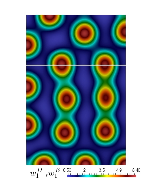
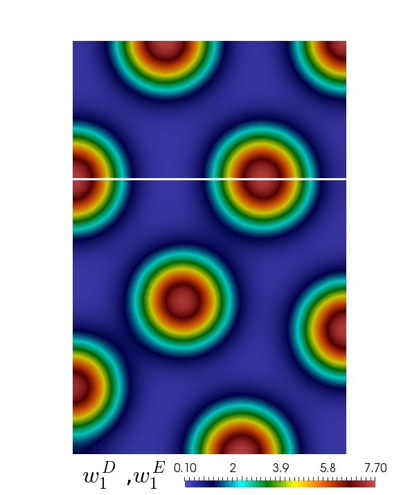
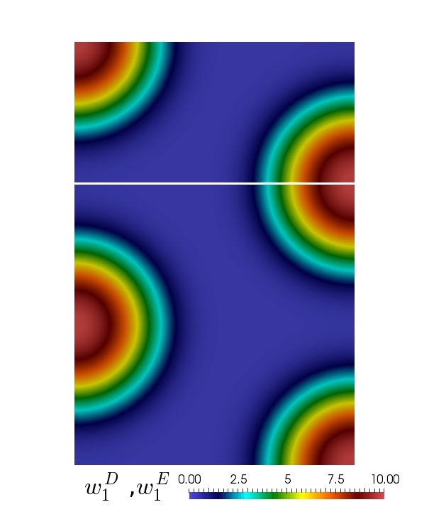
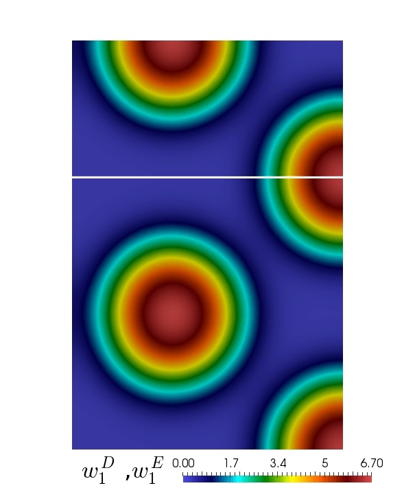
In this example we focus our attention on the effect of cross-diffusion in (2.2). We consider again the Gierer-Meinhardt kinetics (2.3), now decoupled from the linear elasticity equations (2.1). We impose the same reaction parameters on both sides of the interface , , , we set the diffusion coefficients , , and choose the acceleration transmission constants . The domains of interest are the blocks and , which we discretise into unstructured meshes with 16360 and 8032 triangular elements, respectively. Initial concentrations are set according to
where is a uniformly distributed random field with variance . We employ the adaptive time-stepping method described in Algorithm 2 with controller parameters defined as in Table 4.3. We simulate the process until , and display the resulting numerical solutions on Figure 4.1.
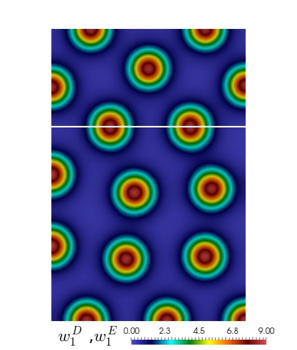
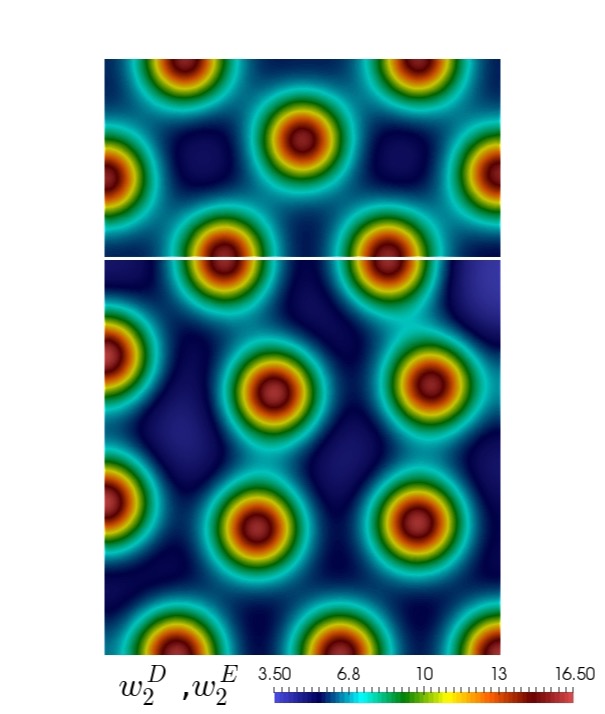
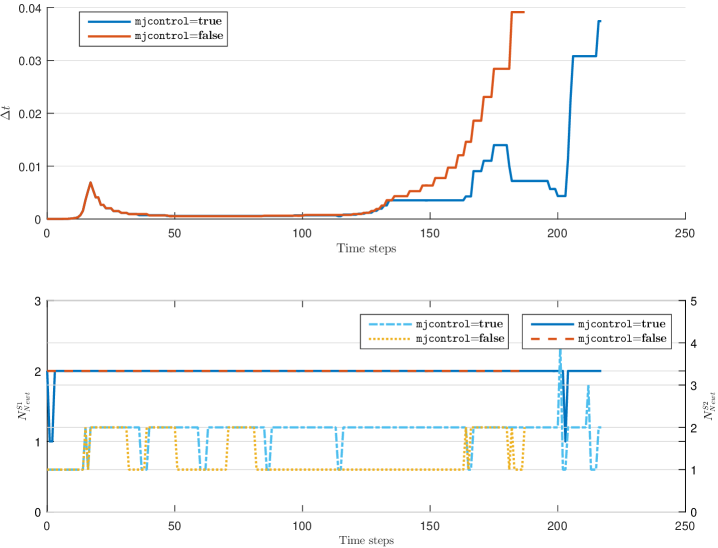
In Figure 4.2 we observe that the adaptive time stepping behaves differently depending on whether one reuses or not the Newton iteration matrices over the implicit stages (this feature is turned on/off by the parameter mjcontrol). For each case, we observe an increase of as the system reaches a steady state. The spatial patterns generated by the two approaches practically coincide and therefore are not shown. However, we observe that the case does not show a marked increase of the timestep when the system reaches stationary patterns. Additionally, we observe that reusing the iteration matrix leads to a slight increase in the number of Newton iterations in the S2 stage.
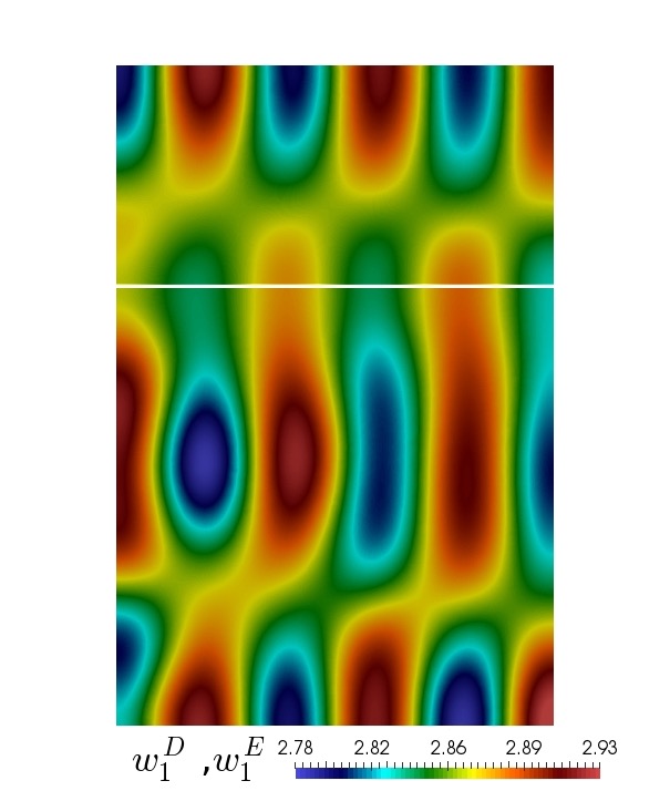
In addition, we test our algorithm for both linear and nonlinear cross-diffusion terms defined as
or
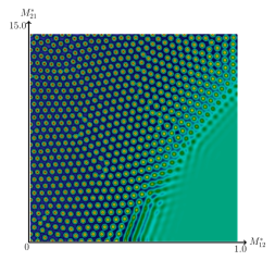
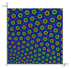
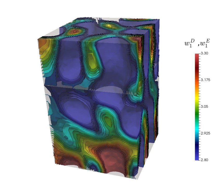
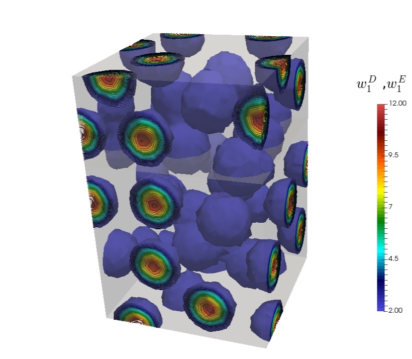
where , () are real constants. For these simulations we impose , . As illustrated in Figure 4.3, the final patterns adopt different structures according to the cross-diffusion matrix employed. While the specific nonlinear cross-diffusion matrix modifies the size of -concentration spots without changing its structure, the linear one (and depending on the parameter values) can change from spots to striped patterns. Furthermore, nonlinear cross-diffusion induces a more visible impact on the distance between high concentration regions, when compared to the linear case. Space-parameter plots illustrate this phenomenon in Figure 4.4. For both cross-diffusion models, we vary spatially the values , , and and from 0 to 1; always checking that the cross-diffusion matrices remain positive definite. The linear cross-diffusion particularly affects the type of patterns that are generated but does not significantly change length scale of the pattern. Nonlinear diffusion, on the other hand, affects directly the pattern length scale without altering the general pattern structure produced by the system. These observations are confirmed in 3D domains as well (cf. 4.5 ).

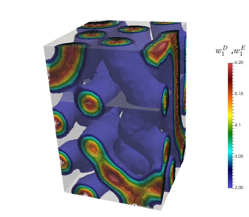
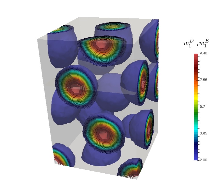
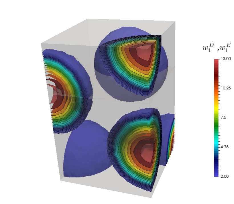
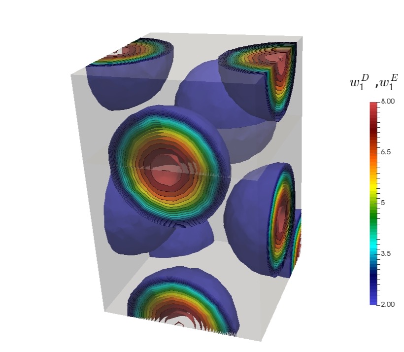
Example 3: A simplified activator-inhibitor model on an elastic 2D domain.
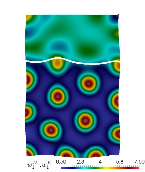
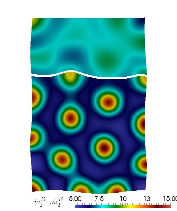
With the objective of testing the time-adaptive algorithms now applied to the mechanochemical coupled problem, we add the elasticity components to the reaction kinetics (2.3) of Example 2 (with the same parameters and mesh). The Young moduli and Poisson ratios defining the material properties of the medium are now , , , . Displacements are prescribed on the boundary according to . Additionally, we impose , and . The medium is initially at rest and stress-free (zero displacement and pressure on the whole domain) and we re-use the initial conditions of the morphogen concentrations defined in the previous test. We use Algorithm 2 with controller parameters defined again as in Table 4.3, except for and . The process is simulated until .
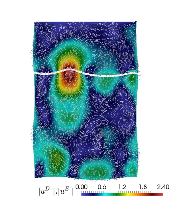
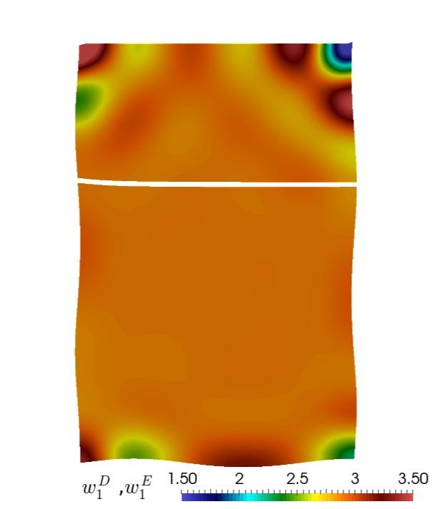
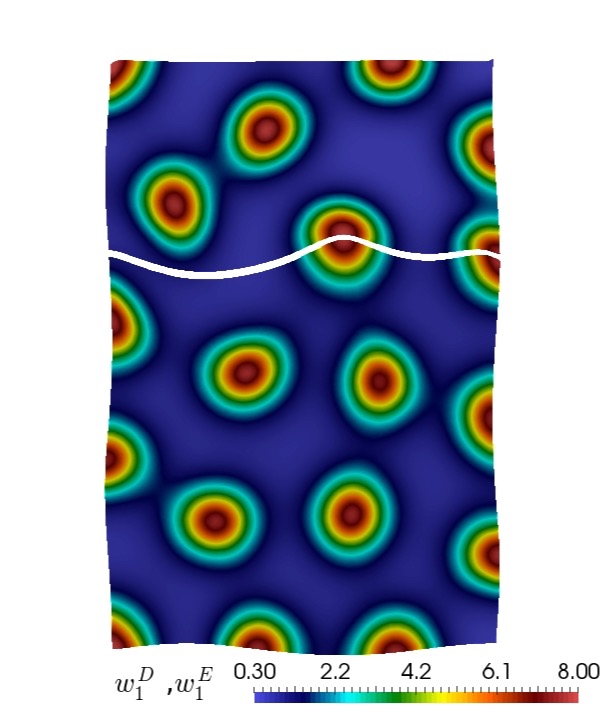
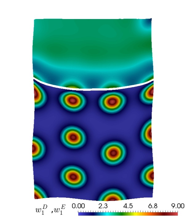
Figure 4.6 presents the final patterns generated by the morphogen concentrations and also the zones of high displacement. On the bottom layer the pattern is similar to the one in Figure 4.1 (in terms of magnitude and spatial structure). For the layer with smaller Poisson ratio, the patterns tend to homogenise and eventually disappear. This phenomenon highlights the effects of mechanical properties on the morphogen dynamics, and we also note that deformations are larger near the interface and close to the bottom boundary of .
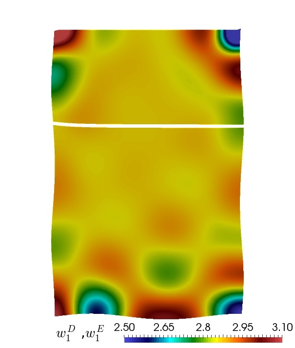
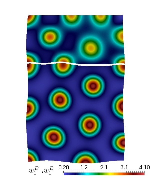
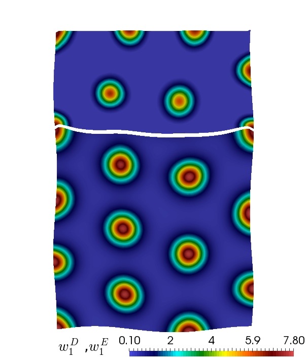
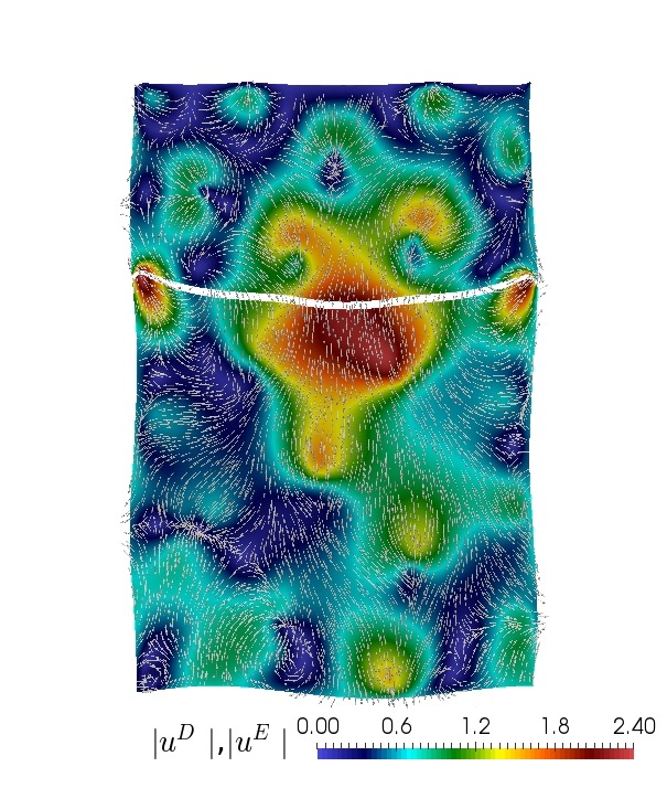
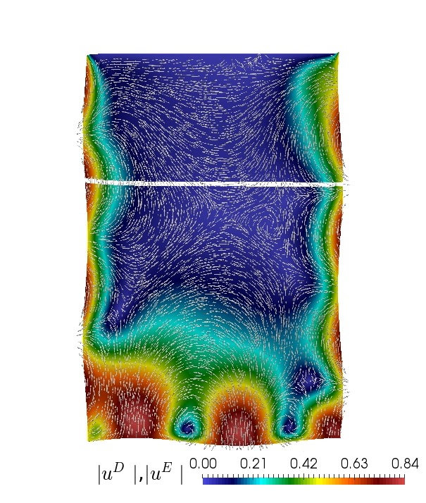
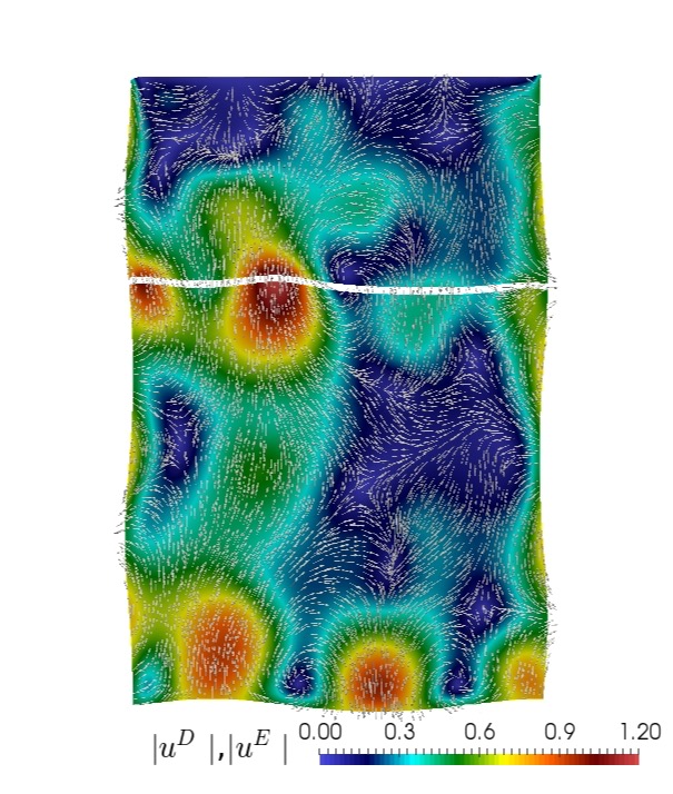
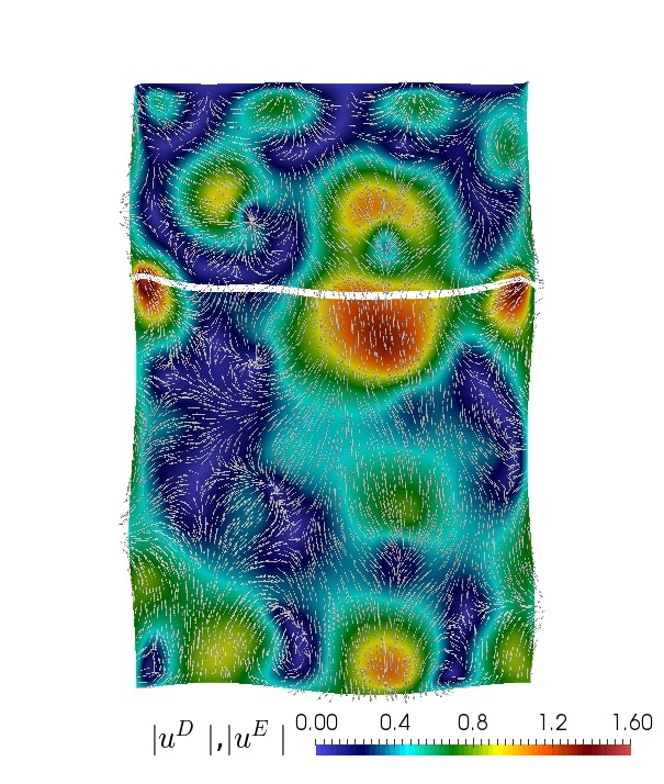
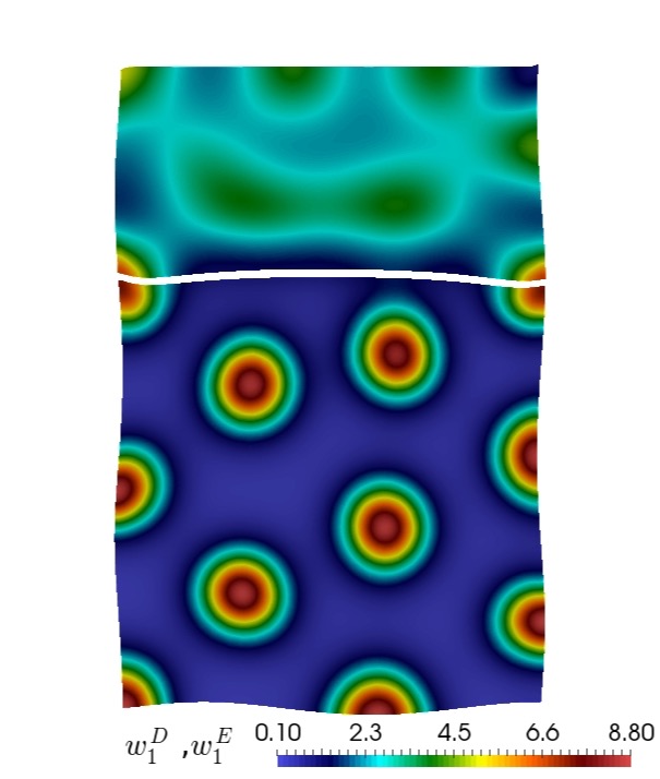
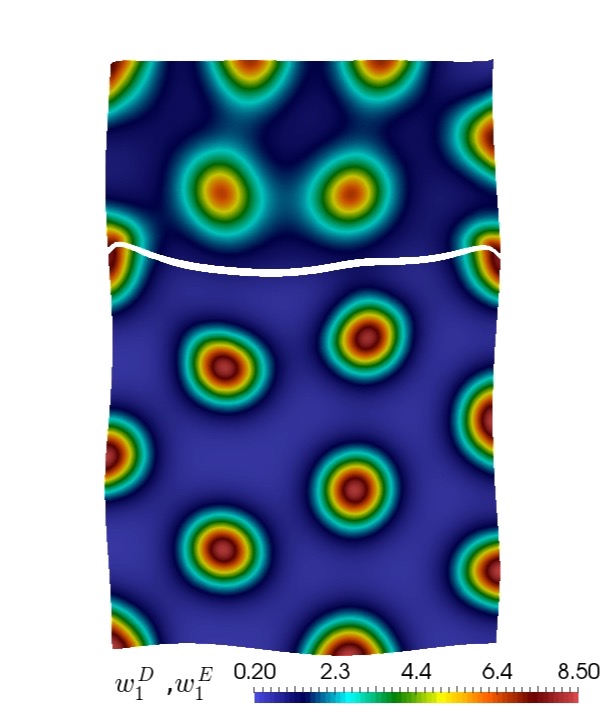
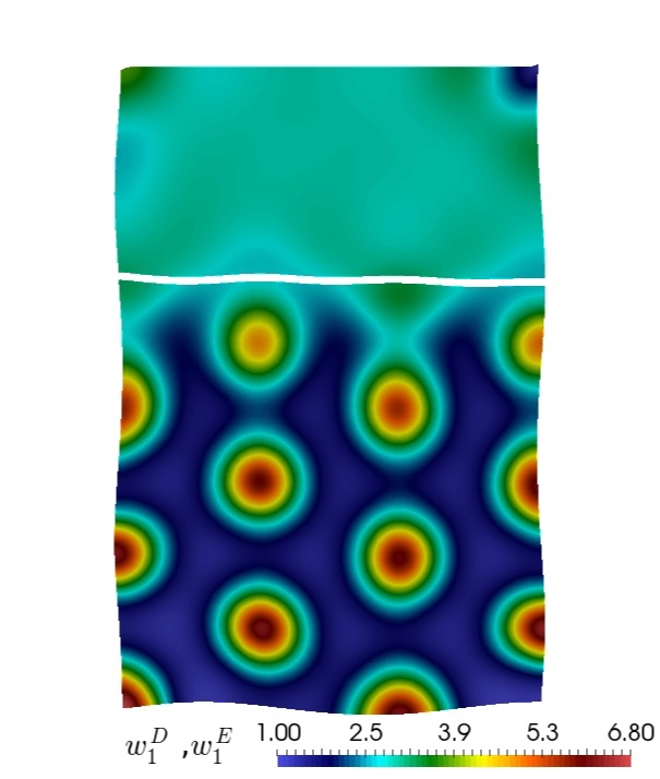
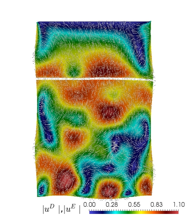
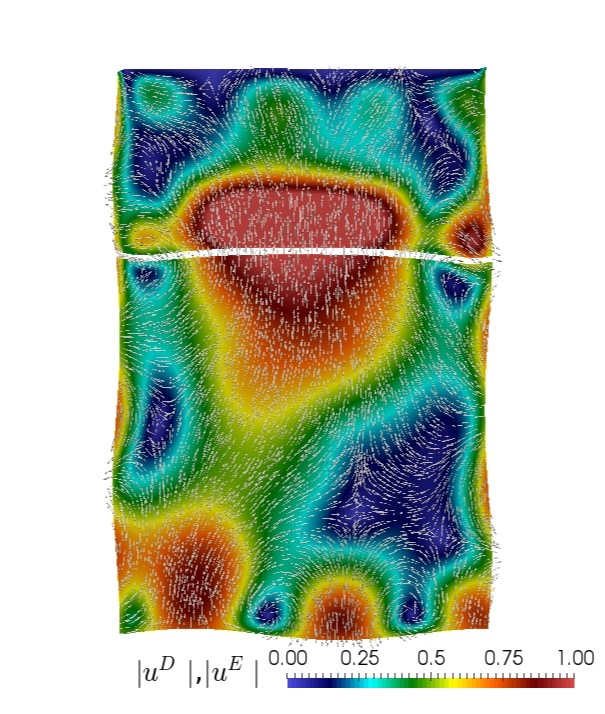
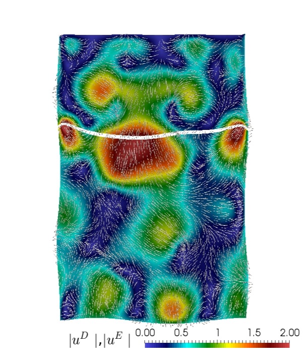
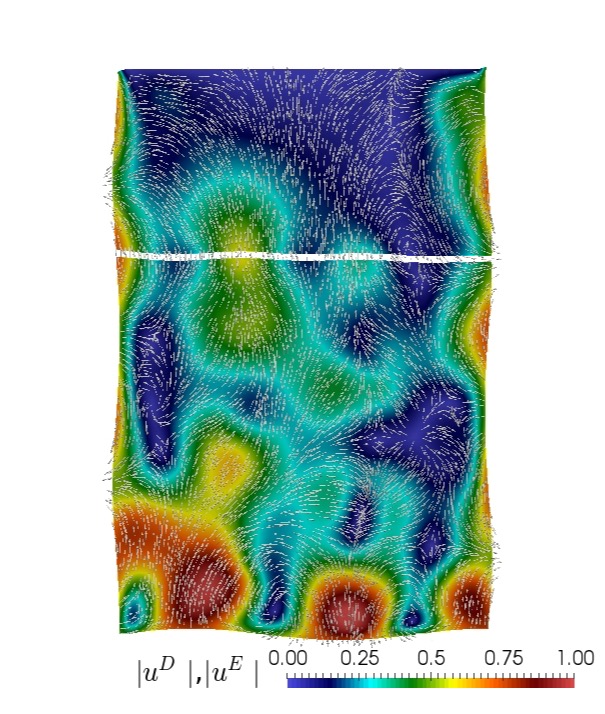
We next test the influence of the reaction and mechanical coupling parameters on the final pattern, and typical results are depicted in Figure 4.7. Perturbations of the ADR coefficients are responsible for considerable variations on the species concentration spatial distribution as well as on the deformation profiles produced by the model. For instance, we observe that the size and shape of morphogens concentration patterns induce differences on the deformation of the interface . Conversely, differences on the mechanical response of each subdomain also directly impact on the chemical species distribution, at the interface. Surprisingly, varying the coupling parameters does not substantially impact the length scale but rather make these patterns to disappear altogether.
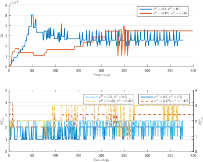
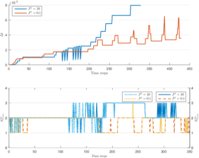
We also inspected the effect of the acceleration constants of the ADR interface conditions together with the degree of material heterogeneity (how different the Lamé parameters are in each subdomain) on the timestep evolution and on the Newton iteration count. For these simulations we fix mjcontrol = true in order to inspect also the efficiency on the update of the Jacobian matrix throughout the simulation. Some of these results are collected in Figure 4.8. The value represents the number of iterations corresponding to accepted timesteps. For this case we observe that is of the order of and progressively increases with the simulation time and the consolidation of the spatial patterns. The algorithm readily detects when the process approaches a steady state, leading to a fast increase of the timestep. However, as show in the case using , this behaviour depends on the choice of model parameters and oscillations might appear, indicating a suboptimal adaptive time stepping. Moreover, changing the value of the acceleration constants may also affect the simulation time, the deformed interface, and the pattern structures. In all our experiments, we observe that accepted steps converge in less than 4 iterations in both stages of the RK method.
Example 4: Simulation of the full-3D appendage model.
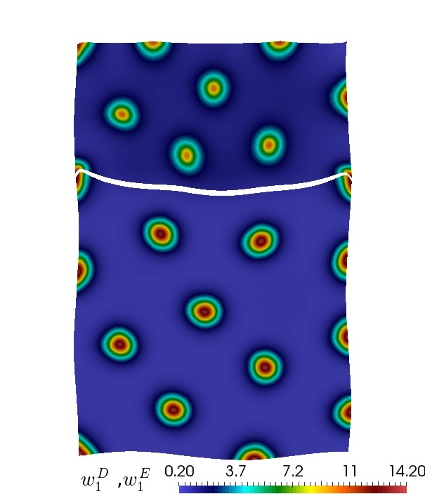
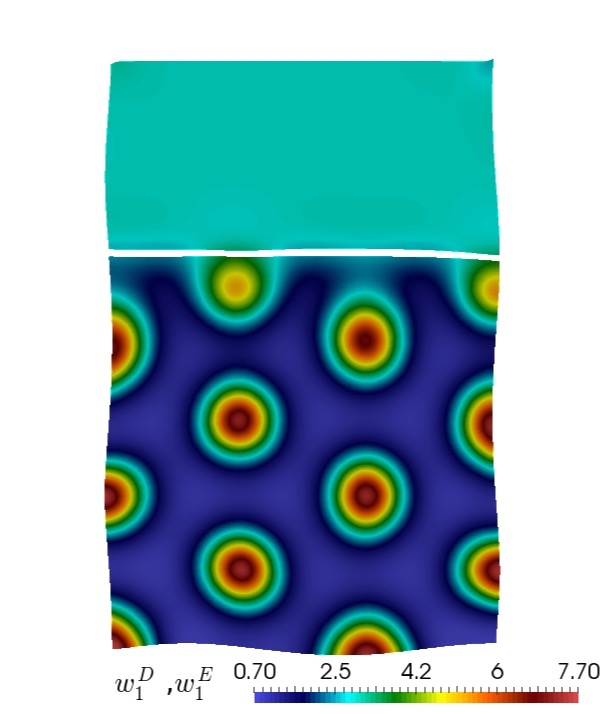
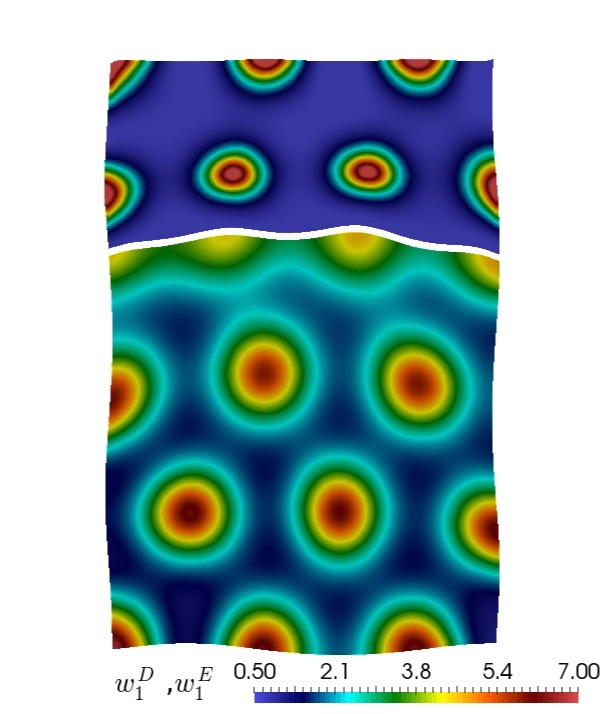
We finally turn to the simulation of the mechanochemical interaction in the context of skin appendage using a 3D slab as computational domain, and focusing on the reaction model proposed in (2.4). Model parameters are chosen according to Table 4.4. The domains of interest are the blocks and , which we discretise into unstructured meshes with 104360 and 60067 tetrahedral elements, respectively. Initial concentrations are set according to steady state solutions obtain from (2.4), perturbed with a uniformly distributed random variable with variance . The adaptive method described in Algorithm 2 is employed with controller parameters as in Table 4.3, except for and . The process is run until .
| , , , , , , , , , , |
| , , , , , , , |
| , , , |
The results are presented in Figure 4.9, showing a clear shift in species (cell, matrix and morphogens) concentration patterns across the interface, with the exception of species (explained by the similarity in the reaction description (2.4)). The uniform Lamé constants on both domains and the Robin conditions imply that deformation patterns are of comparable magnitude throughout , and the zones of high deformations are concentrated near the domain boundary. Different mechanochemical patterns can be produced by changing the coupling and reaction parameters, and a specific study on linear and nonlinear stability will be carried out in a forthcoming contribution. At this stage we can already observe that for , for example, only the dermis species possesses a production term (with logistic growth) while the dynamics on the epidermis is described by a convection-diffusion process. This explains why the concentration variation in the dermis is much smaller than in the epidermis layer. For and we observe a similar behaviour, but having a larger variation on the -axis for a specific layer ( for , for ). This is due to some chemical species being produced only on a specific layer (see (2.4)) and the relevant concentration decreases rapidly, due to metabolism degradation, as one moves away from that layer.
5 Concluding remarks
We have introduced a mechanochemical model for the simulation of basic processes related to skin appendage patterning mechanisms. The two-way coupling between linear elasticity and advection-diffusion-reaction systems is achieved through a mechanical term depending on the gradient of the chemical species, and a pressure-dependent source term representing production of species. A weak formulation in a multidomain setting was introduced, and we presented a partitioned fixed-point and Schwarz algorithm to decouple the system into four principal blocks (the two domains, dermis and epidermis, being treated for advection-diffusion-reaction and mechanics). The space discretisation uses MINI-elements for the approximation of the displacement-pressure pair, and piecewise linear and continuous Lagrange elements for the species concentrations. A trapezoidal BDF2 method combined with adaptive Runge-Kutta schemes is used as a time advancing strategy, and algorithmic details are provided. The convergence properties of the proposed methods were studied in detail, and a set of numerical tests addresses pattern generation and the deformation of the interface.
Anomalous diffusivity (e.g., fractional, stress- or strain-dependent diffusion [14]) was not considered here. Further work is also needed on the detailed linear stability analysis associated to the coupling mechanisms for the specific models at hand, as well as on the application of the developed methods in the simulation of more complex phenomena. Future work will also address extension of our model to non-linear elasticity and viscoelasticity and theoretical considerations on the convergence properties of partitioned and monolithic schemes.
References
- [1] L. Ahtiainen, S. Lefebvre, P.H. Lindfors, E. Renvoisé, V. Shirokova, M.K. Vartiainen, I. Thesleff, and M.L. Mikkola, Directional cell migration, but not proliferation, drives hair placode morphogenesis. Develop. Cell (2014), 28(5):588–602.
- [2] R. Allena, J.J. Muñoz, and D. Aubry, Diffusion-reaction model for Drosophila embryo development. Comput. Methods Biomech. Biomed. Engrg. (2013), 16(3):235–248.
- [3] A. Aman and T. Piotrowski, Cell migration during morphogenesis, Dev. Biol. (2010), 341(1):20–33.
- [4] B. Andreianov, M. Bendahmane, A. Quarteroni, and R. Ruiz-Baier, Solvability analysis and numerical approximation of linearized cardiac electromechanics, Math. Models Meth. Appl. Sci. (2015), 25(05):959–993.
- [5] D.N. Arnold, F. Brezzi, and M. Fortin, A stable finite element for the Stokes equations. Calcolo (1984), 21:337–344.
- [6] A. Badugu, C. Kraemer, P. Germann, D. Manshykau, and D. Iber, Digit patterning during limb development as a result of the BMP-receptor interaction, Sci Rep. (2012), 2:991.
- [7] R.E. Bank, W.M. Coughran Jr, W. Fichtner, E.H. Grosse, D.J. Rose, and R.K. Smith, Transient simulation of silicon devices and circuits, IEEE Trans. Comput.-Aided Design (1985), 4:436–451.
- [8] R. Becker, E. Burman, and P. Hansbo, A Nitsche extended finite element method for incompressible elasticity with discontinuous modulus of elasticity, Comput. Methods Appl. Mech. Engrg. (2009), 198:3352–3360.
- [9] F. BenBelgacem, L.K. Chilton, and P. Seshaiyer, The -mortar finite-element method for the mixed elasticity and Stokes problems, Comput. Math. Appl. (2003), 46:35–55.
- [10] L. Bonaventura and A. Della Rocca, Unconditionally strong stability preserving extensions of the TR-BDF2 method, J. Sci. Comput. (2017), 70:859–895.
- [11] M. Buck, O. Iliev, and H. Andrä, Multiscale finite element coarse spaces for the application to linear elasticity, Central Eur. J. Math. (2013), 11(4):680–701.
- [12] W. Chen, X. Xu, and S. Zhang, On the optimal convergence rate of a Robin-Robin domain decomposition method, J. Comput. Math. (2014), 32(4):456–475.
- [13] A. Chertock, K. Fellner, A. Kurganov, A. Lorz, and P.A. Markowich, Sinking, merging and stationary plumes in a coupled chemotaxis-fluid model: a high-resolution numerical approach, J. Fluid Mech. (2012), 694:155–190.
- [14] C. Cherubini, S. Filippi, A. Gizzi, and R. Ruiz-Baier, A note on stress-driven anisotropic diffusion and its role in active deformable media, J. Theor. Biol. (2017), 430(7):221–228.
- [15] G.C. Cruywagen and J.D. Murray, On a tissue interaction model for skin pattern formation, J. Nonl. Sci. (1992), 2(2):217–240.
- [16] R. Dillon and H.G. Othmer, A mathematical model for outgrowth and spatial patterning of the vertebrate limb bud, J. Theor. Biol. (1999), 197:295–330.
- [17] N. Di-Poï and M.C. Milinkovitch, The anatomical placode in reptile scale morphogenesis indicates shared ancestry among skin appendages in amniotes, Sci. Adv. (2016), 2(6).
- [18] V. Dolean, P. Jolivet, and F. Nataf, An Introduction to Domain Decomposition Methods. Algorithms, Theory, and Parallel Implementation, SIAM Philadelphia, PA, USA (2015).
- [19] J.D. Edwards, J.E. Morel, and D.A. Knoll, Nonlinear variants of the TR/BDF2 method for thermal radiative diffusion, J. Comput. Phys. (2011), 230:1198–1214.
- [20] F. Hecht, New development in FreeFem++, J. Numer. Math. (2012), 20(3-4):251–265.
- [21] M.J. Gander, F. Magoules, and F. Nataf, Optimized Schwarz methods without overlap for the Helmholtz equation, SIAM J. Sci. Comput. (2002), 24:38–60.
- [22] G.N. Gatica, B. Gomez-Vargas, and R. Ruiz-Baier, Analysis and mixed-primal finite element discretisations for stress-assisted diffusion problems, Comput. Methods Appl. Mech. Engrg. (2018), 337.
- [23] G.N. Gatica and W.L. Wendland, Coupling of mixed finite elements and boundary elements for a hyperelastic interface problem, SIAM J. Numer. Anal. (1997), 34(6):2335–2356.
- [24] A. Gierer and H. Meinhardt, A theory of biological pattern formation, Kybernetik (1972), 12:30–39.
- [25] J.D. Glover, K.L. Wells, F. Matthäus, K.J. Painter, W. Ho, J. Riddell, J.A. Johansson, M.J. Ford, C.A.B. Jahoda, V. Klika, R.L. Mort, and D.J. Headon, Hierarchical patterning modes orchestrate hair follicle morphogenesis, PLOS Bio. (2007), 15(7):1–31.
- [26] P. Gosselet and C. Rey, Non-overlapping domain decomposition methods in structural mechanics, Arch. Comput. Methods Engrg. (2007), 13(4):515–572.
- [27] E. Hairer, S.P. Nørsett, and G. Wanner, Solving Ordinary Differential Equations I, Nonstiff Problems. Springer Series in Computational Mathematics. Springer New York, 2008.
- [28] E. Hairer and G. Wanner, Solving Ordinary Differential Equations II, Stiff and Differential-Algebraic Problems. Springer Series in Computational Mathematics. Springer New York, 2010.
- [29] M.E. Hosea and L.F. Shampine, Analysis and implementation of TR-BDF2, Appl. Num. Math. (1996), 20(1):21–37.
- [30] T. Lecuit and P.-F. Lenne, Cell surface mechanics and the control of cell shape, tissue patterns and morphogenesis, Nat. Rev. Mol. Cell. Biol. (2007), 8(8):633–644.
- [31] P. Lenarda, M. Paggi, and R. Ruiz Baier, Partitioned coupling of advection-diffusion-reaction systems and Brinkman flows, J. Comput. Phys. (2017), 344:281–302.
- [32] P.L. Lions, On the Schwarz alternating method. III: a variant for non-overlapping subdomains, In: T.F. Chan, R. Glowinski, J. Périaux, and O. Widlund, editors, Third International Symposium on Domain Decomposition Methods for Partial Differential Equations, held in Houston, Texas, March 20-22, 1989, Philadelphia, PA, 1990. SIAM.
- [33] R.T. Liu, S.S. Liaw, and P.K. Maini, Two-stage Turing model for generating pigment patterns on the leopard and the jaguar, Phys. Rev. E (2006), 74(1):011914.
- [34] D. Manoussaki, A mechanochemical model of angiogenesis and vasculogenesis, ESAIM: Math. Model. Numer. Anal. (2003), 37(04):581–599.
- [35] M. Mercker, F. Brinkmann, A. Marciniak-Czochra, and T. Richter, Beyond Turing: mechanochemical pattern formation in biological tissues, Biol. Dir. (2016), 11(1):22–37.
- [36] S.E. Millar, Molecular mechanisms regulating hair follicle development, J. Inv. Derm. (2002), 118(2):216–225.
- [37] S.A. Montandon, A.C. Tzika, A.F. Martins, B. Chopard, and M.C. Milinkovitch, Two waves of anisotropic growth generate enlarged follicles in the spiny mouse, EvoDevo (2014), 5:33.
- [38] P. Moreo, E.A. Gaffney, J.M. García-Aznar, and M. Doblaré, On the modelling of biological patterns with mechanochemical models: Insights from analysis and computation, Bull. Math. Biol. (2010), 72:400–431.
- [39] J.D. Murray and G.F. Oster, Generation of biological pattern and form, IMA J. Math. Appl. Med. Biol. (1984), 1(1):51–75.
- [40] J.D. Murray, P.K. Maini, and R.T. Tranquillo, Mechanochemical models for generating biological pattern and form in development, Phys. Reports (1988), 171(2):59–84.
- [41] J.D. Murray, Mathematical Biology II: Spatial Models and Biomedical Applications. Interdisciplinary Applied Mathematics. Springer New York, 2006.
- [42] T. Oliver, J. Lee, and K. Jacobson, Forces exerted by locomoting cells, Cell Biol. (1994), 5(3):139–147.
- [43] G.F. Oster, J.D. Murray, and A.K. Harris, Mechanical aspects of mesenchymal morphogenesis, Development (1983), 78(1):83–125.
- [44] K.J. Painter, G.S. Hunt, K.L. Wells, J.A. Johansson, and D.J. Headon, Towards an integrated experimental–theoretical approach for assessing the mechanistic basis of hair and feather morphogenesis, Interface Focus (2012), 2(4):433–450.
- [45] M. Pawlaczyk, M. Lelonkiewicz, and M. Wieczorowski, Age-dependent biomechanical properties of the skin, Postepy. Dermatol. Alergol. (2013), 30(5):302–306.
- [46] M. Ptashnyk and B. Seguin, Homogenization of a system of elastic and reaction-diffusion equations modelling plant cell wall biomechanics, ESAIM: Math. Model. Numer. Anal. (2016), 50(2):593–631.
- [47] A. Quarteroni and A. Valli, Domain Decomposition Methods for Partial Differential Equations, Oxford Science Publications, Oxford (1999).
- [48] C. Remani, Numerical Methods for Solving Systems of Nonlinear Equations, 2012, Lakehead University, Thunder Bay, Ontario, Canada.
- [49] R. Ruiz-Baier, Primal-mixed formulations for reaction-diffusion systems on deforming domains, J. Comput. Phys. (2015), 299:320–338.
- [50] S. Sick, S. Reinker, J. Timmer, and T. Schlake, WNT and DKK Determine Hair Follicle Spacing Through a Reaction-Diffusion Mechanism, AAAS (2006), 314(5804):1447–1450.
- [51] L.J. Shaw and J.D. Murray, Analysis of a model for complex skin patterns, SIAM J. App. Math. (1990), 50(2):628–648.
- [52] H. Shoji, A. Mochizuki, Y. Iwasa, M. Hirata, T. Watanabe, S. Hioki, and S. Kondo, Origin of directionality in the fish stripe pattern, Dev. Dyna. (2003), 226(4):627-633.
- [53] A.E. Shyer, A.R. Rodrigues, G.G. Schroeder, E. Kassianidou, S. Kumar, and R.M. Harland, Emergent cellular self-organization and mechanosensation initiate follicle pattern in the avian skin, Science (2017), 357(6353):811–815.
- [54] G. Søderlind, Automatic control and adaptive time-stepping, Num. Alg. (2002), 31(1):281–310.
- [55] L. Qin and X. Xu, Optimized Schwarz methods with Robin transmission conditions for parabolic problems, SIAM J. Sci. Comput. (2008), 31:608–623.
- [56] A. Quarteroni, T. Lassila, S. Rossi, and R. Ruiz-Baier, Integrated Heart – Coupling multiscale and multiphysics models for the simulation of the cardiac function, Comput. Methods Appl. Mech. Engrg. (2017), 314:345–407.
- [57] A. Tosin, Mechanics and chemotaxis in the morphogenesis of vascular networks, B. Math. Biol. (2006), 68(7):1819–1836.
- [58] L. Tranqui and P. Tracqui, Mechanical signalling and angiogenesis. The integration of cell–extracellular matrix couplings, C.R. Acad. Sci. (2000), 323(1):31-47.
- [59] A.M. Turing, The chemical basis of morphogenesis, Phil. Trans. R. Soc. London B (1990), 237:37–72.
- [60] B.L. Vaughan, R.E. Baker, D. Kay, and P.K. Maini, A modified Oster-Murray-Harris mechanical model of morphogenesis, SIAM J. Appl. Math. (2013), 73:2124–2142.
- [61] M.A. Wyczalkowski, Z. Chen, B.A. Filas, V.D. Varner, and L.A. Taber, Computational models for mechanics of morphogenesis, Birth Defects Res. (2012), 92(6):132–152.
- [62] B. Wang, K. Xia, and G.W. Wei, Matched interface and boundary method for elasticity interface problems, J. Comput. Appl. Math. (2015), 285:203–225.