Lidar Cloud Detection with Fully Convolutional Networks

Abstract

In this contribution, we present a novel approach for segmenting laser radar (lidar) imagery into geometric time-height cloud locations with a fully convolutional network (FCN). We describe a semi-supervised learning method to train the FCN by: pre-training the classification layers of the FCN with image-level annotations, pre-training the entire FCN with the cloud locations of the MPLCMASK cloud mask algorithm, and fully supervised learning with hand-labeled cloud locations. We show the model achieves higher levels of cloud identification compared to the cloud mask algorithm implementation.

1 Introduction

The vertical distribution of clouds from active remote sensing instrumentation is a widely used data product from global atmospheric measuring sites. The presence of clouds can be expressed as a time versus vertical height binary cloud mask (cloud 1, no cloud 0) and is a primary input for climate modeling efforts and cloud formation studies. Ground-based lidars have routinely been employed to provide these cloud masks. Current cloud detection algorithms used to retrieve these masks from lidar data, however, do not always accurately identify the cloud boundaries and tend to oversample or over-represent the cloud. This translates as uncertainty for assessing the radiative impact of clouds and tracking changes in cloud climatologies. Additionally, such algorithms require significant effort to develop and maintain and are sensitive to instrument changes and accurate instrument calibration.

Machine learning has only recently been applied to the atmospheric science domain and in particular cloud retrievals from lidar data. Previous applications of machine learning to lidar data have been primarily focused on airborne lidar instruments for tasks such as estimating vegetation height and canopy cover [15] and estimating forest biomass [5]. Recently, a neural network was trained to detect clouds from satellite data, but in a limited setting with supervised learning [6]. However, deep learning techniques have not been used for cloud detection from ground-based lidar instruments.

In our work, we present a method for using FCNs to detect clouds from MPL data that surpasses an implementation of the well-established Wang and Sasson cloud mask algorithm [17]. We develop a semi-supervised learning method to train the FCN, involving pre-training the “classification” weights of the model with image-level annotations and pre-training the entire model with noisy annotations. We demonstrate the trained FCN model performs better than the established algorithm and verify our learning methodology improves the model performance compared to only using end-to-end supervised learning.

The remainder of this paper is organized as follows. In section 2, we introduce the lidar system and data used for this study. In section 3, we discuss some related work on using FCNs for image segmenation and semi-supervised learning methods. Section 4 outlines the preprocessing of our training and test data and sections 5 and 6 describe our model architecture and training methodology. Section 7 describes and analyzes our cloud segmentation results. We conclude with some suggestions for future work in section 8.

2 Dataset

For this study we use lidar data from micropulse lidar (MPL) systems deployed by the the Atmospheric Radiation Measurement (ARM). The MPL system operate by emitting a low energy laser pulse (~10 $\mu$J) combined with high pulse rate (2500 Hz). Pulses are emitted in an alternating linearly and circularly polarized state and each return signal that is scattered back is collected using a photon detector. The return signal from each pulse is time-resolved to provide the vertical height of the aerosol particles or cloud droplets that are responsible for the scattering. These return signals measured by the photon detector are processed and combined to then provide vertical profiles of the atmospheric structure as attenuated backscatter. Additionally, the linear depolarization ratio (LDR) can be calculated from the linear and circularly return signals to help determine cloud phase (liquid, ice or mixed) as well distinguishing aerosol and clear air. A detailed description of the MPL data processing is given by Campbell et al. [2] and the calculation of the LDR is provided in Flynn et al. [4].

The MPL data stream used is sgp30smplcmask1zwangC1 from the Southern Great Plains (SGP) C1 facility located near Lamont Oklahoma [13]. This location is selected because this observatory is the world’s largest and most extensive climate research facility and focal point for modeling and forecasting efforts. We selected data from January 2010 to December 2016 to train the model. One 30smplcmask1zwang data file contains a 24-hour period of lidar profiles at 30 second temporal resolution and 30 m vertical resolution out to 18km (667 x 2880 data points). We use the total attenuated backscatter, linear depolarization ratio (LDR) as well as a cloud mask product using an algorithm based on Wang and Sassen [17]. The implemented algorithm relies in part on the strong change in the slope of the backscatter that is observed in the presence of clouds and distinguishing clouds from noise or an aerosol layer by inspecting the ratio of extinction of the lidar signal to the backscatter [14]. This cloud mask product, MPLCMASK, is used to compare the model’s performance and pre-train the model.

3 Related work

An FCN is a neural network that contains convolutional layers, but no fully-connected layers. Long et al. [10] show how FCNs can be used to accurately segment images semantically with pixel-to-pixel predictions. The advantage of FCNs is they can be trained with end-to-end, pixel-to-pixel operations which increase learning and inference and allow for fusion of finer and coarser features to help performance [10]. Several applications of FCNs in scientific domains include: biomedical imaging for cells [12], brain tumor segmentation [7], uranium particle identification from mass spectrometry imagery [16], and mitigating radio frequency interference signals in radio data [1]. We use an image-segmentation approach with an FCN model for several reasons. First, it is easy to translate our problem, identify clouds from MPL data, to an image segmentation problem. The input data can be treated as an image by having each measurement act as a color channel. Then, our “image” is a two-channel image, with the backscatter as one channel and the LDR as the other. Then, the problem becomes segmenting the input image for regions of clouds and as previously stated, FCN’s have been very successful performing pixel-by-pixel image segmentation. Visual interpretation of cloud features in lidar images is very similar to a segmentation approach, which takes advantage of global and local features within an image thus suggesting FCNs are an appropriate and natural choice.

An advancement in deep convolutional networks for image segmentation has been the use of weakly-supervised and semi-supervised learning techniques to train the networks. Hong et al. [8] proposes a deep neural network consisting of a classification network, a segmentation network, and bridging layers connecting the two networks. By separating the network, they train each part of the network independently, training the classification network with image-level annotations and the segmentation network with full image semantic segmentations. Their semi-supervised approach is competitive against other semi- and weakly-supervised trained models. Papandreou et al. [11] uses weakly (bounding-box and image-level) annotated images to train deep convolutional neural networks. They show that training with a small amount of pixel-level annotated images combined with a large amount of weakly annotated images results in performance very close to that of training on only pixel-level annotations. Similarly, Weihman et al. [18] demonstrated using end-to-end unsupervised learning as a pre-training step on FCNs produces models that perform statistically similar to their fully supervised counterparts. By adding a reconstruction output layer, their model is able to use the reconstruction loss as weighted component of the loss function and slowly transition to the segmentation loss during training. The advantage of these techniques is models can be trained using large amounts of unlabeled and weakly labeled data while requiring minimal ground truth data. This is applicable to our work since manually create a binary cloud mask for lidar data is a time and labor intensive process, resulting in a small dataset of hand-labeled data. Leveraging these training methodologies removes the need for large datasets of hand-labeled cloud masks without sacrificing model performance.

4 Data preprocessing and preparation

Figure 1: Example of MPL backscatter profile (left) and LDR (right). From January 1st, 2015 (time bins 0-880).

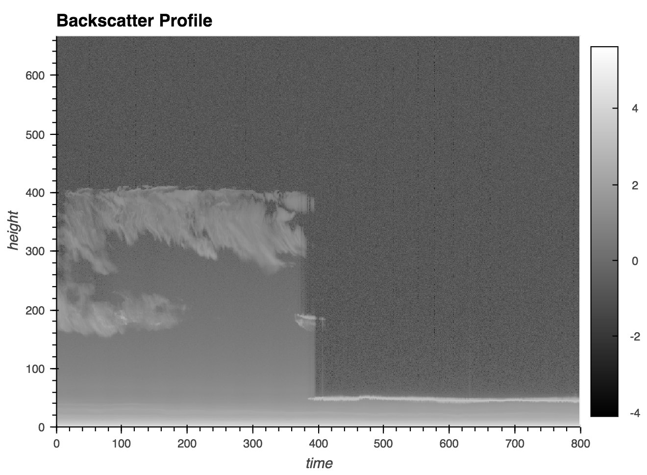
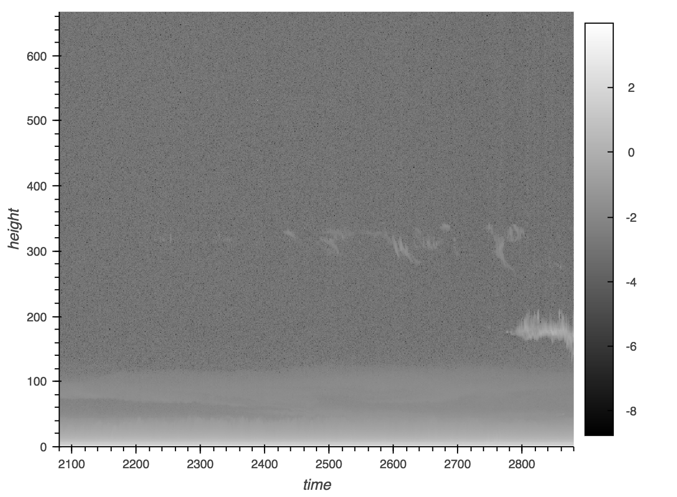
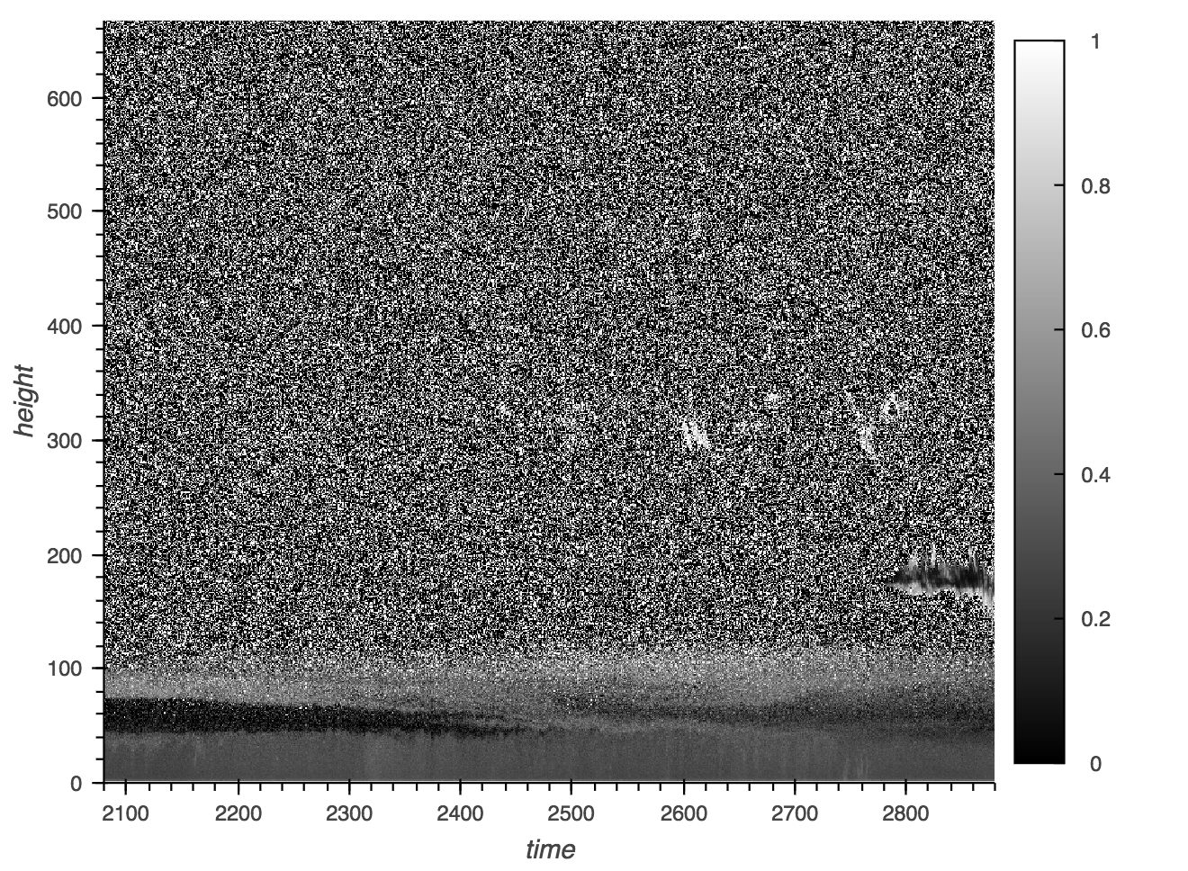
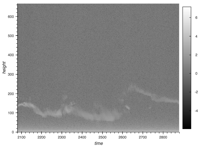
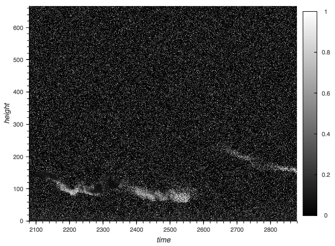
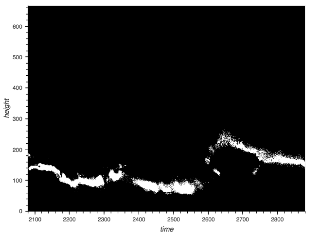
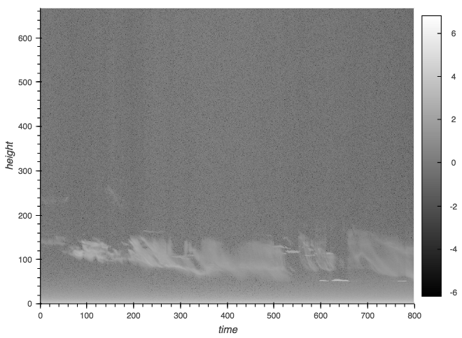
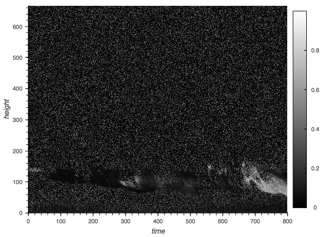
To improve the visualization of the lidar imagery we take the log of the attenuated backscatter. Any missing values, infinite values, or not-a-number (NaN) values are then set to the daily minimum value. Each day is then zero-centered by subtracting the mean from the backscatter and normalized by dividing by the standard deviation of the backscatter mean. The LDR valid data range is between 0 and 1. Missing values and NaNs are set to 0, any values greater than 1 are set to 1 and values less than 0 are set to 0. Figure 1 shows an example of the backscatter and LDR images.

To train and test the model, 82 days of ground truth are hand labeled by a lidar expert with extensive experience with the MPL data. This ground truth consists of cloud masks that have been labeled using the attenuated backscatter and LDR measurements to visually identify the cloud locations. There are 54 days (30 from January 2015, 24 from February 2015) are used for training and validation and 28 (March 2015) are held out for testing.

Given the small amount of hand-labeled data, we increase the amount of data eightfold by splitting each day into quarters time-wise with some overlap (667 x 800) and adding the horizontally flipped version of each quarter day to the dataset. The data was split so that each quarter mostly identified a unique part of the profile and to have max-pooling operations reduce the time dimension more evenly. The quarter days are determined by: time bins 0-800, time bins 680-1480, time bins 1400-2200, and time bins 2080-2880.

We divide the data into four separate disjoint datasets for training and testing:

Classification dataset   For pre-training the classification part of the model, a set of 1780 quarter days is used with image-level annotations identifying whether the quarter days contains clouds. A quarter day is marked as containing clouds if the MPLCMASK contains clouds. It is acceptable to use the MPLCMASK to identify if the quarter day has cloud since the main issue with the product is that it oversamples the cloud boundaries, not misidentify whether clouds exist at a given time. Thus, the product can still capture whether there are clouds in the image. The dataset is divided evenly between quarter days with clouds (890) and without clouds (890).

Noisy dataset   For pre-training the entire model, a set of 4200 quarter days is used (4000 with clouds, 200 without clouds). The ground truth data for this set is the MPLCMASK product. We treat the MPLCMASK product as noisy annotations, since the mask oversamples the shape of the clouds and merges cloud boundaries. No hand-labeled days used for training are included in this dataset.

Hand-labeled dataset   The dataset for supervised training and fine-tuning the model consists of 432 quarter days (362 with cloud, 70 without). This consist of the January and February 2015 lidar data. The ground truth data for this set is the hand-labeled data.

Holdout dataset   Finally, the March 2015 hand-labeled data is used as a hold-out dataset to test the full segmentation model results. This consists of 224 quarter days (172 with cloud, 52 without).

5 Model architecture

Figure 2: Diagram of classification neural network trained to identify if lidar data has a cloud

We use the U-net model design [12] as our base FCN model architecture. The U-net design consists of downsampling the input image then upscaling back to the original size in a series of convolutional layers and deconvolutional layers. In the same spirit of the Hong et al. decoupled network [8], the model is divided into two parts during training: the classification part of the model and the segmentation part.

5.1 Classification model

The model input is the quarter day backscatter profiles and LDR data (667 x 800 x 2). The first layer is a 28 x 1 convolution with stride of 1 that reduces the data size to 640 x 800 x 2. The initial size reduction is done to ensure the downsampling (and later on upsampling) dimension changes are consistent throughout the entire model. Next are five convolutional-pooling blocks. Each block contains two 3 x 3 convolutions layers with stride of 1 with rectified linear unit (ReLU) activation function and a 2 x 2 max pooling layer with dropout. The first convolutional layer doubles the depth size in each block except for the first one, which increase the depth size from 2 to 16. This is followed by a 20 x 25 convolutional layer with stride of 1 with ReLU and dropout to flatten the layer. Next are two dense layers, the first using batch normalization and ReLU and the second using a softmax activation function to reduce to a 1 x 2 output. The first index in the output array is the probability the input data does not contain a cloud and the seconds is the probability the input data contains a cloud. Figure 2 shows the classification model.

5.2 Segmentation model

Figure 3: Diagram of fully convolutional neural network trained to identify clouds from lidar data

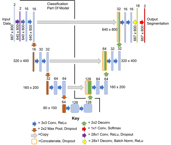
The segmentation model architecture uses the same structure as the classification model up to and including the last 80 x 100 x 128 convolutional output (excluding the max-pooling and dropout layer). The convolutional output is connected to three deconvolutional blocks. Each deconvolutional block consists of a deconvolutional layer that upsamples the image size by 2 and reduces the number of filters by a factor of 2. This is concatenated with the output of the last convolutional layer of the same image size as the output of the deconvolution layer, followed by two 3 x 3 convolutional layers. These "skip" connections help transfer higher level features from earlier convolutions later in model training. We use a 28 x 1 deconvolution layer with batch normalization and ReLU activation to return the data to the initial time and height dimensions (667 x 800). Finally, the model performs a 1 x 1 convolutional layer with softmax activation function to create the output layer. The output layer is the softmax probability for each time-height point whether it is a cloud or not a cloud. A point is identified as being a cloud if it has a probability greater than or equal to 50% of being a cloud. Figure 3 shows the full segmentation model and notes the layers from the classification model that are reused.

6 Training

The FCN model is trained in three stages. First, the classification model in figure 2 is trained using the image-level annotations from the classification dataset. Then, we transfer the classification weights from the model (the weights from the layers on the "classification" side in figure 3) to the segmentation model. Second, we pre-train the FCN segmentation model with the noisy annotations of the noisy dataset. This is similar to using unsupervised pre-training, since it involves training the model on data that is not the desired output to improve the overall performance. However, unsupervised pre-training tends to involve reconstructing the input data for the output while the noisy annotations (the MPLCMASK product) are semantically related to the desired output (the hand-labeled cloud mask). By transferring the weights of the classification model and training on the noisy annotations, we reduce the segmentation search space of the entire model to make it easier to train the model with a limited sample of full segmentation labels. Finally, the FCN segmentation model is trained and fine-tuned using the hand-labeled dataset with the hand-labeled cloud mask as ground truth.

Training for the classification weights and pre-training the segmentation model is done over 100 epochs and fine-tuning the segmentation model is done over 300 epochs. We did not deem it necessary to train the classification model or pre-train the entire model for longer than 100 epochs, since we are transferring the weights from the training steps and the end goal is not the best cloud classification model or a mimic of the MPLCMASK product. We use a batch size of 32 for pre-training the classification model and 10 for pre-training and training the segmentation model. We use accuracy for the loss function of the classification model and categorical cross entropy for the loss function of the segmentation model. Each training step uses an Adam optimizer [9] and a 70-15-15 train-val-test split of the dataset.

Table 1: Best hyper-parameters for each model training

Training step	learning rate	dropout	decay rate
1) Image-level annotation	0.001	0.5	0.0
2) Noisy annotation	0.00059	0.2	0.0
3) Hand-labeled annotations	0.001	0.0	0.0

In each training phase, we perform a hyperparameter search over the learning rate, dropout, and decay rate. For each set of models in the search, we keep the weights from the epoch where the model has the best validation score (accuracy for classification model, F1-score for segmentation model). Then, we select the model with the highest validation score. For the final training step, the selected model is the one with best F1-score on the hold-out dataset. Table 1 lists the best parameters for each training step.

For the FCN segmentation model, we use precision (% of predicted clouds that are actual clouds), recall (% of clouds that are predicted as clouds), and F1-score (harmonic mean of the precision and recall) as our performance metrics. Each of the metrics are calculated over the entire dataset, and not per input image. We use F1-score for the segmentation model instead of accuracy since only a very small set of the time-height points in the hand-labeled ground truth are labeled as clouds. In the hold-out dataset, only %5.79 of points are clouds and in the hand-labeled dataset, only %4.65 of points are clouds. As such, the accuracy measurement (sum of the true positive clouds and true negative non-clouds divided by the total number of points) gets skewed extremely high because the number of non-cloud points heavily outweighs the number of cloud points. For example, if there are 100 points of which 90 are non-cloud and 10 are cloud and the model correctly identifies 90 non-cloud and 1 cloud, then the accuracy is 91% despite only correctly identifying 10% of the cloud points.

The model is implemented with the Keras python module [3]. We train the model on a computer cluster with Dual Intel Broadwell E5-2620 v4 @ 2.10GHz CPUs node with 64GB 2133Mhz DDR4 memory and dual NVIDIA P100 12GB PCI-e based GPUs.

7 Results

Table 2: Model performance on test split of hand-labeled dataset

Method	F1-Score	Precision	Recall
MPLCMASK product	0.5892	0.4423	0.8795
No pre-training	0.792	0.7301	0.8653
No noisy annotation pre-training	0.8126	0.7795	0.8487
FCN segmentation model	0.8777	0.8637	0.8998

Table 3: Model performance on holdout dataset (March 2015)

Method	F1-Score	Precision	Recall
MPLCMASK product	0.65	0.5072	0.9049
No pre-training	0.8263	0.7801	0.8783
No noisy annotation pre-training	0.8242	0.7938	0.857
FCN segmentation model	0.8508	0.8336	0.8687

Overall, the FCN segmentation model outperforms the MPLCMASK product. For the test split of the hand-labeled dataset (table 2) and the holdout dataset (table 3), the FCN model has an F1-score of 0.8777 and 0.8508, respectively. This exceeds the performance of the MPLCMASK (0.5892 and 0.65, respectively). The FCN model precision is almost double, indicating the model correctly identifies more clouds than the MPLCMASK product by a factor of 2. Thus, the model is able to captures more of the cloud detail in the output than the MPLCMASK. We note that the FCN model slightly underperforms against the algorithm in recall in the holdout dataset (0.8687 and 0.9049, respectively), but outperforms the algorithm in the test split (0.8998 and 0.89, respectively).

(a) backscatter

(b) ldr

(c) hand-labeled

(d) model

(e) MPLCMASK

Figure 4: Cloud segmentation results for several days (top to bottom: March 13th, March 16th, March 26th, 2015). (a): MPL backscatter profile. (b): MPL linear depolarization ratio. (c): hand-labeled cloud mask. (d): segmentation model output. (e): MPLCMASK cloud mask.

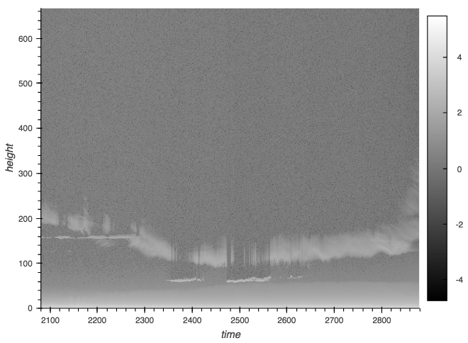
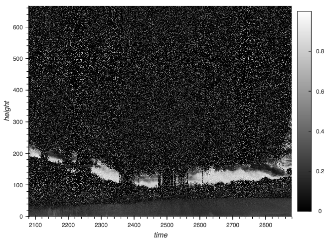
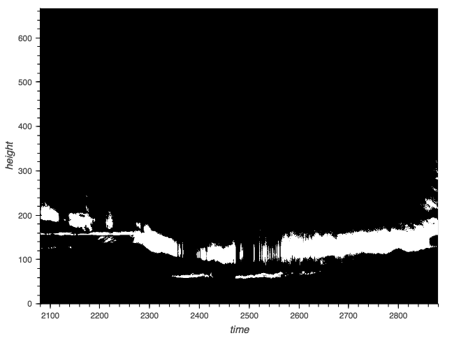
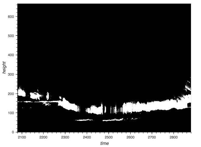
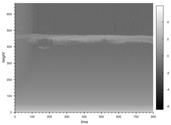
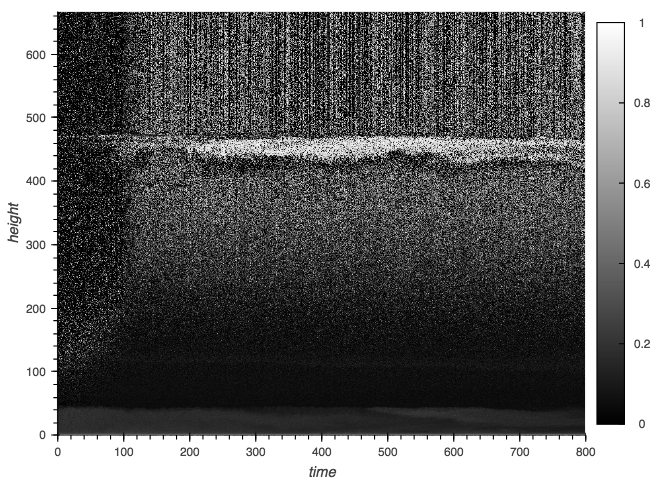
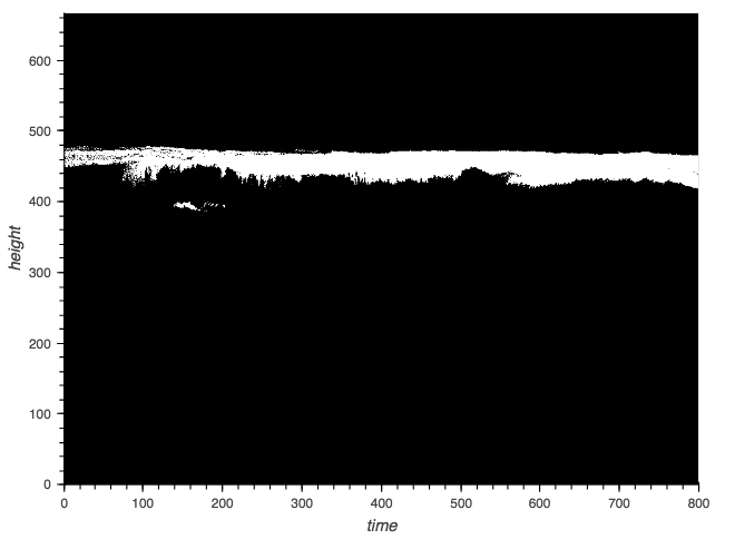
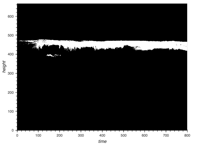
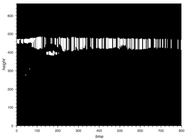
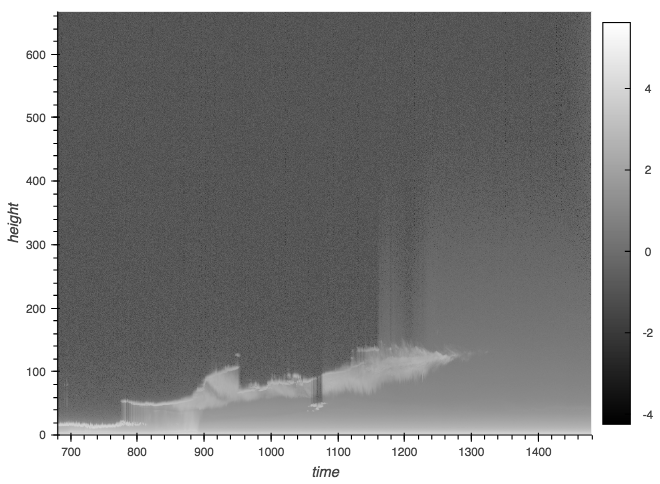
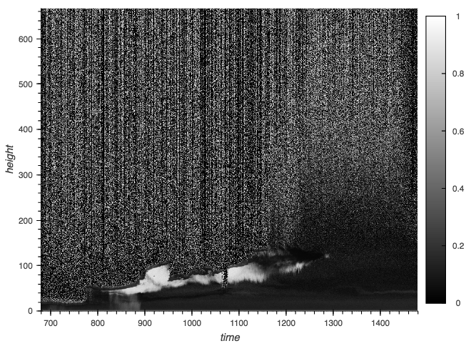
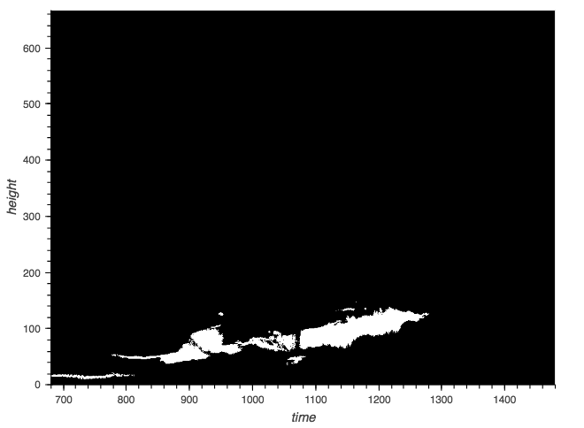
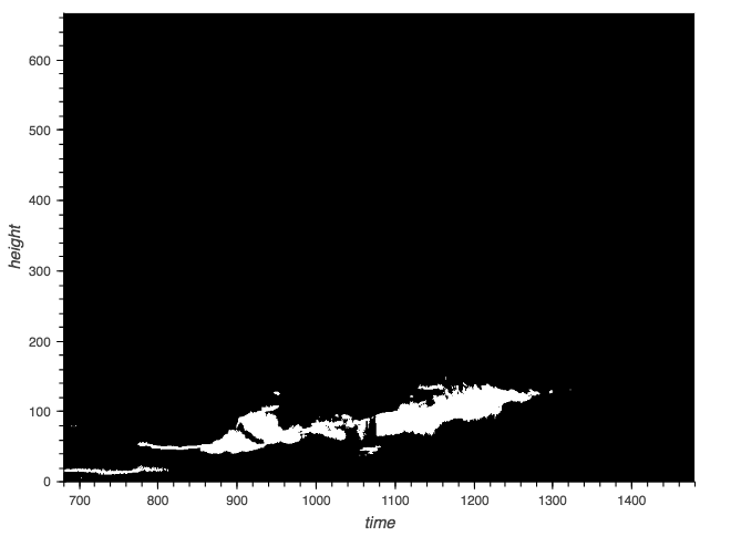
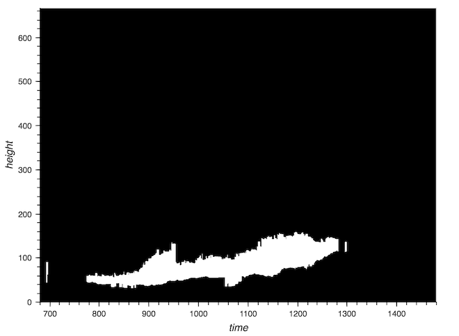
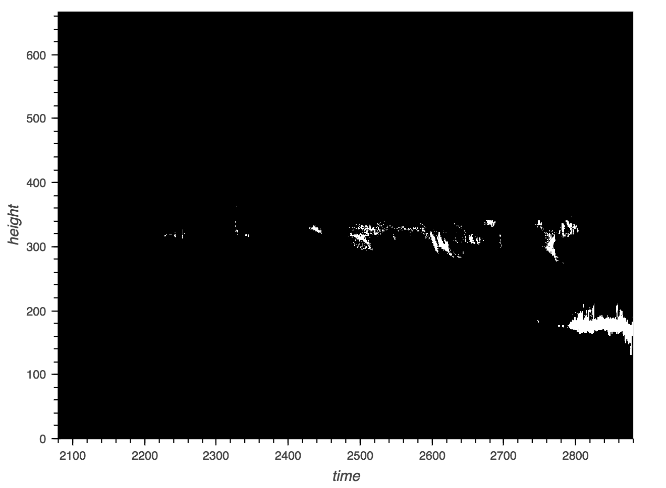
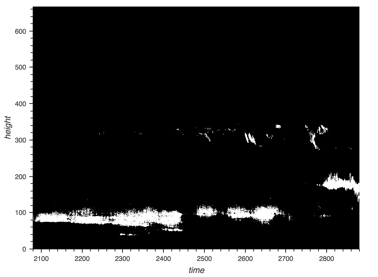
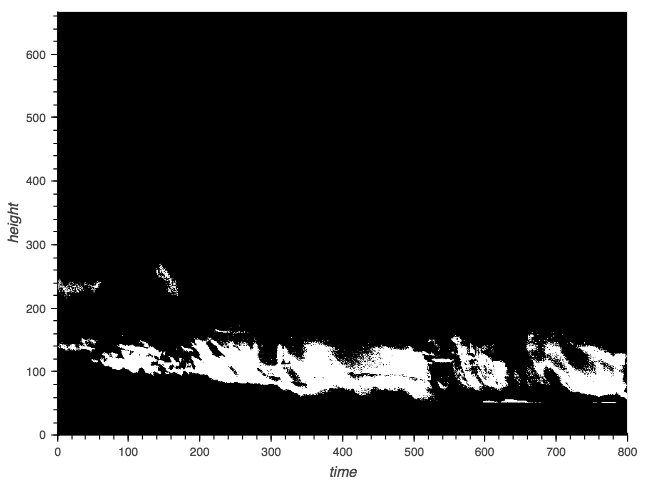
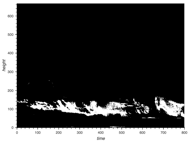
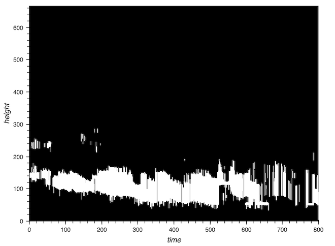
Figure 4 presents several qualitative results from the FCN model. As shown, the clouds identified by the model closely follow that of the hand-labeled mask. In the first and third examples (March 13th and March 26th), the model output is more detailed in contrast to the MPLCMASK product, which tends to exaggerate the cloud shape and size and merge multiple cloud layers. In the second example (March 16th), the MPLCMASK is unable to consistently detect the cloud layer as indicated by the vertical gaps in the mask.

7.1 Training methodology verification

To verify the training methodology, we train a FCN model without the first two training steps (i.e., no image-level and noisy annotation pre-training) and one without the second training step (no noisy annotation pre-training). For the second model, we use the same classification weights that were transferred to the best FCN model during the first training step. Additionally, we use the same hyperparameter search techniques to find the best model. As seen in table 3 (rows 2 and 3), both of these models have lower F1-scores (0.8263 and 0.8242) and precision (0.7801 and 0.7938) than the fully trained FCN model on the hold-out dataset. We do note the FCN model with no pre-training does have a slightly higher recall (0.8783) than the fully trained model. On the test-split of hand-labeled dataset, the fully trained FCN model outperforms both of them in each category (see rows 2 and 3 of table 2). Thus, the pre-training with the image-level and noisy annotated data increases the model’s overall performance.

(a) backscatter

(b) ldr

(c) hand-labeled

(d) model

(e) MPLCMASK

Figure 5: Cloud segmentation results for March 30th, 2015. (a): MPL backscatter profile. (b): MPL linear depolarization ratio. (c): hand-labeled cloud mask. (d): segmentation model output. (e): MPLCMASK cloud mask.

7.2 Misidentified aerosol-dust layers

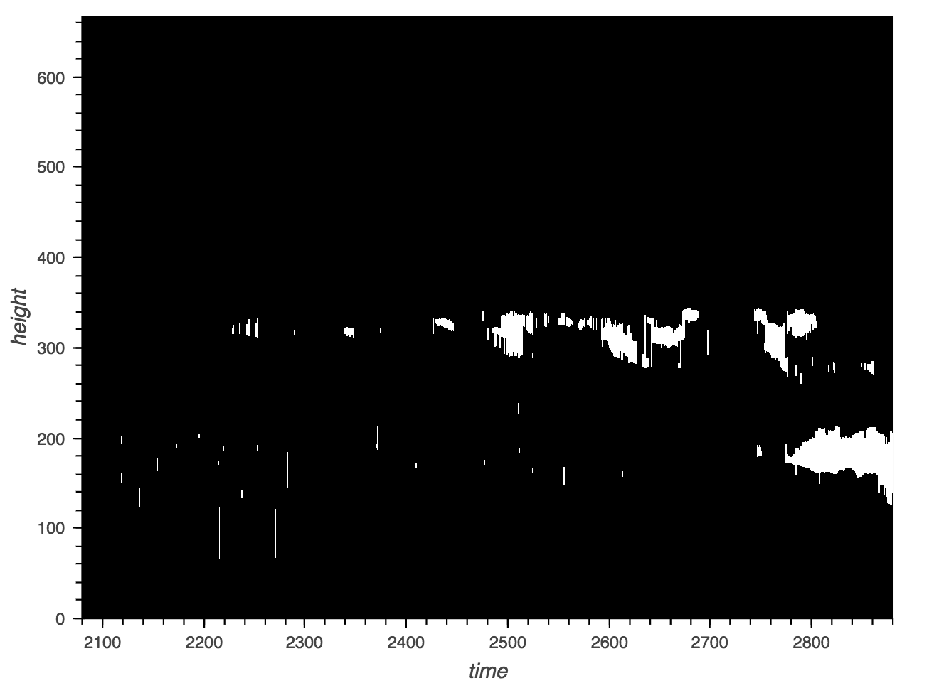
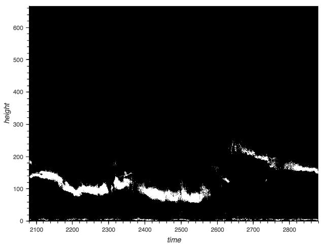
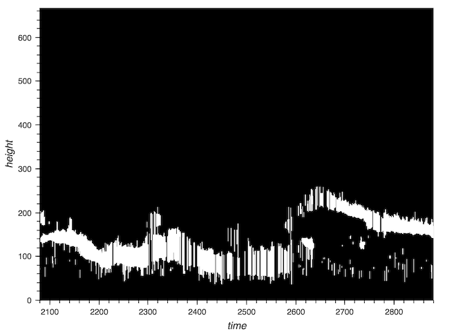
In the holdout dataset (March 2015), we discovered one day, last quarter of March 30th 2015, where the model performs very poorly (f1-score: 0.2929, precision: 0.1806, recall: 0.7752). The model incorrectly marks a layer in the lower height bins (see figure 5) as cloud. The attenuated backscatter of the scatterers in this layer visually appears similar to aerosol but the LDR values are close to that of an ice leading the model to label the layer cloud. This layer is not observed in images from a ceilometer, a second co-located lidar system at the SGP, on this same day. The ceilometer has a longer wavelength and is less sensitive to detecting smaller particles such as aerosol. This suggest this layer is likely aerosol, possibly related to local agricultural activity. Looking closer at the training data, there are no days in January or February 2015 that had similar aerosol layers. Thus, the model did not have the opportunity to train on these edge cases and did not learn to ignore this layer.

(a) backscatter

(b) ldr

(c) hand-labeled

(d) model

(e) MPLCMASK

Figure 6: Model results for MPL data at the Oliktok site: Top row is May 11th, 2016 (bins 2080 to 2880), bottom row is May 13, 2015 (bins 0 to 800). (a): MPL backscatter profile. (b): MPL linear depolarization ratio. (c): hand-labeled cloud mask. (d): segmentation model output. (e): MPLCMASK cloud mask.

7.3 Test on MPL data from different facility

In addition, we test the FCN model on MPL data from the ARM Oliktok mobile facility on the north slope of Alaska to see how well the model performs on data from a different site location [13] since different sites have different atmospheric properties and weather that can affect the input data. We randomly select 14 days from May 2016 to hand-label and run the model on. The model performs reasonably well on the Oliktok data, achieving an F1-score of 0.8045 (0.8478 precision, 0.7654 recall). This performs much better than the MPLCMASK product, which has an F1-score of 0.4185 (0.371 precision, 0.48 recall). Several qualitative results can be seen in figure 6. While the FCN model does perform noticeably worse on the Oliktok data in contrast to the holdout data from the SGP site, the results are encouraging. We believe if we use transfer learning and train the model on data from the Oliktok site, we can improve the model’s performance on the Oliktok site data and its overall performance.

8 Conclusion

We successfully use train a FCN to segment clouds from lidar imagery. We show our semi-supervised training method outperformed the MPLCMASK data product and verify it improves the overall performance of the model. Likewise, we analyze model performance on lidar data from different observations sites (mid-latitude versus polar) and potential transfer learning to make the model more robust. Initial results are promising, but requires further investigation. In the future, we want to investigate if data seasonality (winter vs. summer) impacts model training and cloud detection. Another area of interest is applying our model to satellite lidar data from the Cloud-Aerosol Lidar and Infrared Pathfinder Satellite Observation (CALIPSO) satellite and to lidar data from High Spectral Resolution Lidar (HSRL) systems. Furthermore, we are interested in if adding another input data channel, specifically a ceilomoter lidar data, improves model performance.

Acknowledgements

The research described in this work is part of the Deep Science for Scientific Discovery Initiative at Pacific Northwest National Laboratory. It was conducted under the Laboratory Directed Research and Development Program at PNNL, a multiprogram national laboratory operated by Battelle for the U.S. Department of Energy. This research was performed using PNNL Institutional Computing at Pacific Northwest National Laboratory. Also, we would like to thank the Pacific Northwest National Laboratory 2017 Quickstarter Initiative for initial funding for this work. Additionally, we would like to thank the Atmospheric Radiation Measurement (ARM) Data Center for the 30smplcmask1zwang data stream data.

References

- [1] Joel Akeret, Chihway Chang, Aurelien Lucchi, and Alexandre Refregier. Radio frequency interference mitigation using deep convolutional neural networks. Astronomy and computing, 18:35–39, 2017.
- [2] James R. Campbell, Dennis L. Hlavka, Ellsworth J. Welton, Connor J. Flynn, David D. Turner, James D. Spinhirne, V. Stanley Scott III, and I. H. Hwang. Full-time, eye-safe cloud and aerosol lidar observation at atmospheric radiation measurement program sites: Instruments and data processing. Journal of Atmospheric and Oceanic Technology, 19(4):431–442, 2002.
- [3] François Chollet et al. Keras. https://github.com/keras-team/keras, 2015.
- [4] Connor J. Flynna, Albert Mendozaa, Yunhui Zhengb, and Savyasachee Mathurb. Novel polarization-sensitive micropulse lidar measurement technique. Opt. Express, 15(6):2785–2790, Mar 2007.
- [5] Colin J. Gleason and Jungho Im. Forest biomass estimation from airborne lidar data using machine learning approaches. Remote Sensing of Environment, 125:80 – 91, 2012.
- [6] L. Gómez-Chova, G. Mateo-García, J. Muñoz-Marí, and G. Camps-Valls. Cloud detection machine learning algorithms for proba-v. In 2017 IEEE International Geoscience and Remote Sensing Symposium (IGARSS), pages 2251–2254, July 2017.
- [7] Mohammad Havaei, Axel Davy, David Warde-Farley, Antoine Biard, Aaron Courville, Yoshua Bengio, Chris Pal, Pierre-Marc Jodoin, and Hugo Larochelle. Brain tumor segmentation with deep neural networks. Medical Image Analysis, 35:18–31, 2018/03/09 2017.
- [8] Seunghoon Hong, Hyeonwoo Noh, and Bohyung Han. Decoupled deep neural network for semi-supervised semantic segmentation. CoRR, abs/1506.04924, 2015.
- [9] Diederik P. Kingma and Jimmy Ba. Adam: A method for stochastic optimization. CoRR, abs/1412.6980, 2014.
- [10] Jonathan Long, Evan Shelhamer, and Trevor Darrell. Fully convolutional networks for semantic segmentation. In The IEEE Conference on Computer Vision and Pattern Recognition (CVPR), June 2015.
- [11] George Papandreou, Liang-Chieh Chen, Kevin P Murphy, and Alan L Yuille. Weakly-and semi-supervised learning of a deep convolutional network for semantic image segmentation. In Proceedings of the IEEE international conference on computer vision, pages 1742–1750, 2015.
- [12] O. Ronneberger, P.Fischer, and T. Brox. U-net: Convolutional networks for biomedical image segmentation. In Medical Image Computing and Computer-Assisted Intervention (MICCAI), volume 9351 of LNCS, pages 234–241. Springer, 2015. (available on arXiv:1505.04597 [cs.CV]).
- [13] Chitra Sivaraman and Jennifer Comstock. Micropulse lidar cloud mask (30smplcmask1zwang). jan 2010 - dec 2016, 36 36 18.0 n, 97 29 6.0 w; 70 29 42 n, 149 53 9.6 w: Southern great plains central facility (c1), olikiok point (m1), 2011.
- [14] Chitra Sivaraman and Jennifer Comstock. Micropulse lidar cloud mask value-added product technical report. 2011.
- [15] Daniela Stojanova, Panče Panov, Valentin Gjorgjioski, Andrej Kobler, and Sašo Džeroski. Estimating vegetation height and canopy cover from remotely sensed data with machine learning. Ecological Informatics, 5(4):256 – 266, 2010.
- [16] Jay G. Tarolli, Benjamin E. Naes, Lamar Butler, Keeyahna Foster, Caleb M. Gumbs, Andrea L. Howard, and David Willingham. Fully convolutional neural network for removing background in noisy images of uranium bearing particles. Analyst, 142:1499–1511, 2017.
- [17] Zhien Wang and Kenneth Sassen. Cloud type and macrophysical property retrieval using multiple remote sensors. Journal of Applied Meteorology, 40(10):1665–1682, 2001.
- [18] S. Wiehman, S. Kroon, and H. de Villiers. Unsupervised pre-training for fully convolutional neural networks. In 2016 Pattern Recognition Association of South Africa and Robotics and Mechatronics International Conference (PRASA-RobMech), pages 1–6, Nov 2016.