Chemotaxis on networks:
Analysis and numerical approximation
Abstract.
We consider the Keller-Segel model of chemotaxis on one-dimensional networks. Using a variational characterization of solutions, positivity preservation, conservation of mass, and energy estimates, we establish global existence of weak solutions and uniform bounds. This extends related results of Osaki and Yagi to the network context. We then analyze the discretization of the system by finite elements and an implicit time-stepping scheme. Mass lumping and upwinding are used to guarantee the positivity of the solutions on the discrete level. This allows us to deduce uniform bounds for the numerical approximations and to establish order optimal convergence of the discrete approximations to the continuous solution without artificial smoothness requirements. In addition, we prove convergence rates under reasonable assumptions. Some numerical tests are presented to illustrate the theoretical results.
Keywords: Chemotaxis, partial differential equations on networks, global solutions, finite elements, mass lumping, upwind discretization
AMS-classification (2000): 35K15, 35R02, 65M60, 92C17
1. Introduction
Back in the 1970s, Keller and Segel [23] introduced their celebrated model of chemotaxis describing the collective movement of cellular organisms in response to the distribution of a chemical substance. According to [8, 19], the minimal system given by
serves as a prototype for studying many interesting mathematical aspects of chemotaxis. In the context of biological applications, denotes the density of the population of interest and is the concentration of the chemoattractant. The differential equations are usually augmented by homogeneous Neumann boundary conditions which leads to global conservation of the population and to preservation of positivity in both variables.
The analysis of this parabolic-parabolic model of chemotaxis is well understood by now. Local existence of a unique solution was proven by Yagi in [36] and global existence was established by Nagai, Senba, and Yoshida [25] under a smallness condition on the initial data. For large initial mass, blow-up in finite time was demonstrated in [15, 22] for dimension . Finite-time blow-up cannot occur in dimension and thus solutions for the nonlinear parabolic system exist globally in time [18, 28]. We refer to [19, 21] for an overview about various models of chemotaxis and further theoretical results.
Apart from the analysis, also the numerical approximation of chemotaxis models has attracted significant interest in the literature. Nakaguchi and Yagi [26] proposed fully discrete schemes obtained by Galerkin approximation in space and Runge-Kutta methods in time, and they established convergence rates under appropriate smoothness assumptions on the true solution. Filbet [13] studied finite volume approximations and proved convergence also for non-smooth solutions. Higher order schemes have been studied in [7, 11]. In order to retain the conservation of mass and the positivity of the numerical solution, Saito [31] proposed and analyzed an upwind finite element scheme for multidimensional problems; a slightly different approach was considered [32]. Let us also mention recent work [3, 14, 27] concerning the approximation of hyperbolic models of chemotaxis.
In this paper, we study chemotaxis on one-dimensional networks modeled by a system of partial differential-algebraic equations on finite metric graphs [24]. A one-dimensional version of the minimal system is imposed on every edge of the graph and complemented by algebraic coupling conditions at the vertices to ensure continuity of the solution and conservation of mass across junctions. A corresponding system has been proposed and investigated by Borsche et al. [2], who considered a positivity preserving finite volume discretization and established the well-posedness of their scheme. Let us also mention recent work by Camilli and Corrias [6], who considered problems with constant coefficients and proved well-posedness by perturbation arguments and using the mapping properties of the heat semi-group on networks. Numerical methods for hyperbolic models of chemotaxis on networks were investigated by Bretti et al. [5].
Before we proceed, let us briefly discuss the main contributions of our manuscript: By extending the functional analytic framework of Osaki and Yagi [28], we consider the chemotaxis problem on networks as a semilinear parabolic system which allows us to establish existence of a local solution by Galerkin approximation, energy estimates, and perturbation arguments. Following the ideas of [20, 28], we further show that the solution remains positive, provided that the initial values are positive, and we prove that the total mass of the population is conserved for all time. This yields uniform a-priori estimates for the -norm of the density and allows us to derive sharper energy estimates by which we can show that the solution can at most grow polynomially in time and hence exists globally. These results can be seen as a natural generalization of those in [20, 28] to one-dimensional networks. However, we use somewhat different energy estimates in our proofs which allows us to apply our analysis also to problems with discontinuous model parameters and to networks of rather general topology. Our method of proof also differs from that in [6] and our results are more general, in particular, our analysis covers the case of non-constant and discontinuous coefficients. As preparation for the second part of the manuscript, we also establish higher regularity of solutions.
After having proved the global existence and uniqueness of solutions, we turn to their systematic numerical approximation. For the discretization, we here consider a Galerkin approximation in space by finite elements combined with an implicit time-stepping scheme. In order to ensure positivity of the discrete solutions, we employ a mass-lumping strategy and an upwind discretization for the convective term. The resulting scheme has a similar structure as that considered by Saito [31] for chemotaxis problems in multiple dimensions, but the formulation of our scheme is closer to that of the continuous problem, which facilitates the analysis substantially. Some alternative but related approaches can be found in [13] and [32]. Using similar methods of proof as on the analytical level, we derive uniform bounds for the discrete approximations and we establish convergence of the numerical solution and order optimal convergence rates under reasonable smoothness assumptions. Our analysis is somewhat sharper and more general than that presented in [31]. In particular, we do not require a strong restriction on the time step to guarantee the stability of our fully discrete scheme and we obtain convergence in the general case without artificial smoothness assumptions.
The remainder of the manuscript is organized as follows: In Section 2, we introduce our notation and the problem under investigation, and we give a variational characterization of solutions which will be the basis for the rest of the manuscript. In Section 3, we establish the existence and uniqueness of solutions and derive uniform bounds that grow at most polynomially in time. In addition, we prove higher regularity of solutions under natural smoothness and compatibility conditions on the initial data. The numerical approximation is introduced in Section 4 and we establish uniform global bounds for the discrete solutions. In Sections 5 and 6, we prove the convergence of discrete solutions to the true solution and we establish order optimal convergence rates under reasonable smoothness assumptions. For illustration of our theoretical findings, we present some numerical tests in Section 7 and we close the presentation with a short summary and a discussion of possible directions for future research.
2. Preliminaries
We start by introducing our notation and then formally state the chemotaxis problem on the network to be considered for the rest of the paper.
2.1. Network topology
Let be a finite directed and connected graph [1] with vertices and edges . To any edge pointing from vertex to , we set and . The matrix with entries then is the incidence matrix of the graph. For any , we denote by the set of edges starting or ending at , and for we define . We further denote by the set of boundary vertices and call the set of interior vertices. A small example illustrating our notation is presented in Figure 2.1.
2.2. Function spaces
To any edge we associate a positive length and with some abuse of notation, we always identify the topological edge with the geometric interval in the sequel. Let be the vector with entries . Following the notation of [24], we call the triple a metric graph. We further denote by
the space of square integrable functions on which is a Hilbert space when equipped with the natural scalar product
The corresponding norm is given by and the spaces , are defined accordingly. In addition, we will also make use of the function space
consisting of continuous functions with square integrable weak derivatives. This space is complete when equipped with the norm defined by . We denote by the dual space of consisting of continuous linear functionals . Note that by continuity and density, the scalar product can be extended to the duality product on , for which we use the same symbol.
For and some Banach space , we denote by the space of measurable functions with values and with finite norm . Spaces of differentiable functions in time are denoted by and equipped with their natural norms. As usual, we write for convenience. Let us recall that the embedding of the energy space
into is continuous, which can be proven with similar arguments as on single intervals. As a consequence, the evaluation is well-defined for functions and one has a uniform bound
with a constant independent of ; we refer to [12] for details and further references.
2.3. Problem statement
Let be a finite directed metric graph as introduced above. On every edge , the chemotactic movement shall be described by
| (2.1) | |||||
| (2.2) |
with model parameters to be specified below. Recall that denotes the restriction of a function onto the edge . In addition to the above equations, we assume that the solution is continuous across vertices, i.e.,
| (2.3) |
and we require that the population and concentration are conserved at all vertices, i.e.,
| (2.4) | |||||
| (2.5) |
These conditions imply that no mass is gained or lost at interior vertices or across the boundary of the network. To complete the definition of our model problem, we finally assume to have knowledge of the initial values
| (2.6) |
Any pair of sufficiently regular functions , for instance, continuously differentiable in time and twice continuously differentiable in space on every edge, will be called a regular solution of (2.1)–(2.6) on , if it satisfies the equations in a pointwise sense.
2.4. Variational characterization of solutions
Throughout our analysis, we will make use of the following weak characterization of regular solutions.
Lemma 2.1.
Proof.
Let us start with the second identity. Multiplication of (2.2) by a test function on every edge , integration over , and summation over all edges leads to
Via integration-by-parts on every edge , the last term can be transformed to
Note that by definition of . Exchanging the order of summation and using the continuity condition (2.3), which implies that for some and all , the last term can be further evaluated as
For the last equality, we made use of the coupling condition (2.5). A combination of the above formulas already yields the second identity of the lemma, and the first one can be derived with very similar arguments. ∎
Remark 2.2.
The equations (2.7)–(2.8) also make sense for less regular functions, e.g.,
The particular choice of these spaces will become clear from our analysis. Such a pair of functions which satisfies (2.7)–(2.8) for a.a. will be called a weak solution of problem (2.1)–(2.5). Note that the first term in (2.7) has to be interpreted as a duality product here. By standard embedding results [12], one can see that which allows to satisfy the initial values in a reasonable way.
3. Well-posedness
In order to guarantee the existence and uniqueness of solutions of problem (2.1)–(2.6), we make the following assumptions on the parameters and the initial values.
-
(A1)
such that as well as and uniformly a.a. on for some positive constants . For ease of presentation, we additionally assume that the coefficients are constant on every edge .
-
(A2)
and with and
We will denote by the bounds for the coefficients.
3.1. Local solvability
Using standard arguments for semilinear parabolic problems, one can now establish the local well-posedness of the problem under consideration.
Theorem 3.1.
Let (A1)-(A2) hold. Then there exists a time horizon , depending on the geometry of the graph, on the bounds for the coefficients, and inverse monotonically on , , such that the system (2.1)–(2.6) has a unique local weak solution
and the norm of the solution can be bounded by the norm of the initial data.
A detailed proof is given in the appendix. Let us mention already here that the particular functional analytic setting allows to consider (2.1)–(2.6) as a semilinear parabolic system and the result can thus be proven by a fixed-point argument. The positivity of the initial values in assumption (A2) is not required for the local existence.
3.2. Global solutions
As a next step, we now show that the norm of the solution does not blow up in finite time and, therefore, the solution exists globally.
Theorem 3.2.
Similarly as in [20, 28], our proof is based on conservation and positivity preservation of solutions, which we state explicitly as a preparatory result.
Lemma 3.3.
Let (A1)–(A2) hold and let be the local weak solution guaranteed by Theorem 3.1. Then
Moreover, the solution is positive, i.e., and on for a.a. .
Proof.
The first assertion follows by testing (2.7) with . Now let denote the negative part of . Testing equation (2.7) with , we conclude that
From Theorem 3.1, we deduce that for a.a. . Using Lemma A.1, we thus obtain
where only depends on and . Choosing allows to absorb the first term in the left hand side of the energy estimate, and by Lemma A.2, we deduce that
in the last identity we used that . This shows that on its domain of existence. The non-negativity of can then be derived with similar arguments. ∎
Proof of Theorem 3.2
The positivity of the solution is already guaranteed by Lemma 3.3. The remaining proof of the a-priori estimate then proceeds in several steps.
Step 1: As a direct consequence of Lemma 3.3, we obtain that
| (3.1) |
for all . Using this identity, we further deduce from (2.8), by testing with and integration over time, that
| (3.2) |
Note that is a polynomial in whose coefficients depend continuously on the data.
Step 2: Testing (2.8) with yields
Here we used (3.1) and Lemma A.1 for the second estimate, and employed (3.2) and Young’s inequality for the third estimate. Note that is again a polynomial of with coefficients depending continuously on the problem data. By some elementary computations and integration with respect to time, we further obtain
| (3.3) |
with polynomial depending only on and .
Step 3: Testing equation (2.8) with yields the estimate
with and . Here we used Lemma A.1 and (3.1) in the second estimate, and Young’s inequality for the third. By integration in time, we get
| (3.4) |
with constant and polynomial whose coefficients again depend continuously on the data. By squaring the previous estimate, we further get
| (3.5) |
with and . In the derivation of this estimate, we used Hölder’s inequality to bound the term from above.
Step 4: Testing equation (2.7) with leads to
with constant . From (3.4) and (3.5), we can deduce that
Together with the estimate (3.3) and using Young’s inequality, one can then see that
The coefficients of the polynomial again depend continuously on the problem data.
Step 5: Inserting the last expression in the first estimate of Step 4, slightly rearranging the terms, and integrating with respect to time now yields
| (3.6) |
with polynomial whose coefficients depend continuously on the data. This is the required estimate for . A combination with (3.3) and (3.4) yields the bounds for . ∎
3.3. Higher regularity
We now state some bounds for the solution in stronger norms which are obtained under the assumption that the initial values have higher regularity and satisfy the usual compatibility conditions. We thus assume in the following that
-
(A3)
and ,
where is the space of regular fluxes and the space of piecewise smooth functions with appropriate regularity on the individual edges . Under these assumptions, one can show that the solution in fact enjoys higher regularity.
Theorem 3.4.
Let (A1)–(A3) hold. Then the solution of Theorem 3.2 satisfies
| (3.7) | ||||
| (3.8) |
4. Discretization
We now turn to the systematic discretization of the chemotaxis problem on networks by a finite element method in space and an implicit time stepping scheme.
4.1. Notation
Let be the interval represented by the edge and let be a uniform mesh of with subintervals of length . The global mesh is then defined by and is the global mesh size. Furthermore, let , be the vertices of the mesh . We denote by
and the spaces of piecewise polynomials on and , respectively, and by the space of polynomials of degree on the element . Note that , but in general .
For the approximation of the population density and the concentration in space, we consider the finite element space
| (4.1) |
of continuous and piecewise linear functions over the mesh . We further denote by the standard -orthogonal projection onto , defined by
Recall that is uniformly bounded on and on . Moreover,
| (4.2) |
for all with and . These estimates are readily proven by the standard approximation error estimates for the -projection, inverse inequalities, and interpolation arguments; see [4] for details.
Let us now turn to the time discretization. We choose a time step size and set for . For any given sequence , we denote by
| (4.3) |
the backward difference quotient with respect to the given time discretization. Let us note that for any scalar product with associated norm , there holds
which can be verified by some basic calculations. As a direct consequence, one has
| (4.4) |
which will be frequently used to derive discrete energy estimates in our analysis below.
4.2. Auxiliary results
In order to guarantee the positivity of solutions also on the discrete level, some modifications of the standard Galerkin approach will be required. In the following, we introduce the main ingredients and present some basic results.
Quasi-interpolation
For the approximation of the initial values, we will use a quasi-interpolation operator , which is defined by
| (4.5) |
where is the element patch around the vertex of the mesh . Let us recall that the operator is linear and continuous with
| (4.6) |
for all with ; see [4, 9] for details. Moreover, the operator is positivity-preserving, i.e.,
| (4.7) |
which follows directly from the construction (4.5) via local averaging.
Mass-lumping
It is well-known that some sort of mass lumping is required to ensure a discrete maximum principle for the finite element approximation of parabolic problems, see e.g. [33]. To this end, we define for the lumped scalar product
where denotes the linear interpolation of the function . This corresponds to using numerical integration on every element by the trapezoidal rule. One can verify by simple calculations that the induced norm
is equivalent to the standard -norm on the finite element space , i.e.,
| (4.8) |
Upwinding
As a final ingredient for our discretization scheme, we now describe the upwind technique for the convective term. Let be given. Then for any , we define on every element by
| (4.9) |
Note that for any , the operator is linear and bounded, i.e.,
| (4.10) |
Moreover, the piecewise constant function interpolates at the vertices and, therefore, standard Taylor estimates yield
| (4.11) |
for all with a uniform constant independent of the mesh.
4.3. Definition of the discretization scheme
We are now in the position to formulate our numerical approximation scheme for the weak formulation of problem (2.1)–(2.6).
Problem 4.1.
Set , . Then for , find with
| (4.12) | ||||
| (4.13) |
We will show below that the discrete solution is well-defined, that the scheme is positivity preserving, and that the total population is conserved for all time. For our analysis, we will need some auxiliary results which we state next.
4.4. Algebraic properties
Let us start with summarizing some algebraic properties of the discretization scheme (4.12)–(4.13). We denote by the nodal basis of the finite element space defined by
| (4.14) |
Now let be the coordinate vector of the function with respect to this basis given by . From the particular form of the basis functions , one can directly deduce that
| (4.15) |
Moreover, the discretized system (4.12)–(4.13) can be written in algebraic form as
with system matrices defined by
and
From the definition of the matrices, one can immediately deduce the following properties.
Lemma 4.2.
(a) For any , the matrix is diagonal. If , then for all . (b) For with , the matrix satisfies , for , and . (c) Let . Then the matrix satisfies , for all , and .
Proof.
Note that the entries of all system matrices are defined by integrals over the network which can be split into integrals over individual elements respectively.
(a) By definition of the matrix , one has with element contributions given by for . The properties in (a) then follow directly from (4.14).
(b) In a similar manner, we can decompose as with the non-zero entries of for the element given by
and else. The properties in (b) then follow by summation over all elements.
(c) The matrix can again be split into element contributions. Now let for . Then the non-zero entries of are given by
for and else. The properties in assertion (c) then follow directly from these observations by summation over all elements. ∎
4.5. Well-posedness, conservation, and positivity
As a direct consequence of the algebraic properties stated in the previous lemma, we obtain the following result.
Lemma 4.3.
Let (A1)–(A2) hold. Then Problem 4.1 has a unique solution . Moreover, and , for all .
Proof.
Let , denote the coordinate vectors for the functions and . Using (A2), (4.7), (4.15), and the definition of the initial values, one can see that and . Moreover, the algebraic system defining the solution at iteration can be rewritten as
| (4.16) | ||||
| (4.17) |
From the algebraic properties stated in Lemma 4.2 and the assumptions (A1) on the model parameters, one can deduce that the system matrices and are strictly diagonally dominant. This shows that the two linear systems (4.16) and (4.17) can be solved uniquely. Existence of a unique discrete solution for all then follows by induction. From Lemma 4.2, one can further deduce that and have positive entries and that the system matrices and are M-matrices; see [29] for details. By the inverse positivity of M-matrices one can thus infer that and , if and . Positivity of the discrete solution for all then follows by induction and noting that , ; see above. The conservation property finally follows by testing (4.12) with . ∎
Remark 4.4.
A related algebraic argument was used by Saito in [31] to establish positivity of the discrete solution. In that work, however, a strong smallness condition on the time step size was required to ensure that the system matrices are row-wise diagonally dominant. Here we use the fact that the matrices and are column-wise diagonally dominant for any which, together with the sign conditions on the entries, is sufficient to prove the M-matrix property. This allows us to avoid the strong smallness condition on . The same argument should allow to improve the analysis for the method of [31].
4.6. Uniform a-priori bounds
With similar reasoning as on the continuous level, we are now able to derive uniform bounds also for the discrete solutions.
Theorem 4.5.
Let (A1)–(A2) hold and be the solution of Problem 4.1. Then
with a polynomial whose coefficients only depend on the problem data.
Proof.
The proof of Theorem 3.2 applies almost verbatim. In particular, the constants and polynomial functions appearing in the proof are of the same form as those appearing in Theorem 3.2. For convenience of the reader, we repeat the main steps. All estimates will hold uniformly for all time steps .
Step 1: As a direct consequence of Lemma 4.3, we obtain
Without loss of generality we may set by altering either of the two constants in the respective proofs. Testing (4.13) with and using the positivity of , we get
From the uniform bound on and induction, we thus deduce that
Note that the polynomial has the same form as that in the proof of Theorem 3.2.
Step 2: Testing (4.13) with and using (4.4) leads to
with the same polynomial as in the proof of Theorem 3.2. Summation over yields
Step 3: By testing equation (4.13) with and proceeding with the same arguments as in the proof of Theorem 3.2, one arrives at
Squaring this estimate and some elementary estimates further lead to
The constant and the polynomial are again of the same form as those in Theorem 3.2.
Step 4: We now turn to the estimates for . By testing (4.12) with , using (4.4), and proceeding in the same manner as in the proof of Theorem 3.2, we get
From the previous estimates for , we may then further deduce that
and this bound holds with the same polynomial as in the proof of Theorem 3.2.
Step 5: A combination of the estimates in Step 4 now leads to
which yields the desired bound for . The corresponding estimates for then follow by inserting this bound into the estimates of Step 2 and Step 3. ∎
Let us emphasize that all arguments used for the analysis of the problem on the continuous level carry over to the discrete setting almost verbatim. The reason for this is that by its variational character, the proposed method with mass lumping, upwinding, and implicit time integration inherits all important structures of the continuous problem.
5. Convergence
Based on the uniform bounds of the discrete solution provided by Theorem 4.5, we now establish the convergence of the discretization scheme towards the unique solution of the continuous problem without additional regularity assumptions. For a convenient presentation of our results, we will interpret the discrete functions as (piecewise) continuous functions of time. Such extensions will be denoted with double subscripts .
Theorem 5.1.
Proof.
The proof is based on standard arguments for the analysis of nonlinear parabolic problems, see e.g. [30]. We therefore only sketch the main arguments.
Step 1a: Let be piecewise constant in time with values given by and for . Furthermore, let and be piecewise constant in time with values and for . Then from the variational characterization (4.12)–(4.13), one can deduce that
for all test functions and , and for a.a. .
Step 1b: From the a-priori estimates of Theorem 4.5 and the weak compactness of bounded sets in reflexive Banach spaces [30], one may deduce that there exist limit functions and with
as well as
This implies that and in ; see [30] for details.
It remains to show that satisfies (2.7)–(2.8) and that the initial values satisfy and . We start with verifying (2.8).
Step 2a: Recall that denotes the -orthogonal projection onto . Then
By the weak convergence of in , we infer that for all as . From the density of in , the approximation properties of the -projection , and the quasi-uniformity of the mesh , one can see that with . The uniform boundedness of in the norm of therefore yields that for all when . Now let be linear operators defined by
Then by the uniform bounds for the discrete solution and the quasi-uniformity of the mesh , one can see that
for and all . Recall that is the space of piecewise smooth functions. Thus, the family of linear operators is uniformly bounded on and for which is dense in . Hence, for all by the Banach-Steinhaus theorem [16]. In summary, we thus have shown that
for all and all as . It then follows from Lebesgue’s differentiation theorem [12] that
for all and for a.a. .
Step 2b: In a similar manner, one can show that
for all and for a.a. . This shows that satisfies equation (2.8).
We next turn to the verification of identity (2.7).
Step 3a: With the very same arguments as above, one can show that
for all and for a.a. as . It thus remains to establish the convergence for the convective term, which we do next.
Step 3b: Let us define linear operators by
Then from the uniform bounds for the discrete solution , the -stability of the -projection on the quasi-uniform mesh , and (4.10), one can deduce that
This shows that the family of operators is uniformly bounded for all . As a next step, we decompose
By the Aubin-Lions lemma [30], we know that in . Moreover, in and in . This implies that
for all and for any test function . From the estimate (4.11), we therefore deduce that . Using the -stability of the -projection and the uniform a-priori bounds for the discrete solution , one can then see that
In summary, we thus have shown that
for all . With the assertions of Step 3a, this shows that solves (2.7).
Step 4: From the estimates for the quasi-interpolation operator stated in Section 2, one can deduce that in for all . Together with the continuity of the trace mapping for the space , this yields and .
6. Error estimates
Under suitable smoothness assumptions on the true solution, we can now also derive quantitative convergence rates. The aim of this section is to prove the following result.
Theorem 6.1.
Let (A1)–(A3) hold and assume that the solution of (2.1)–(2.6) satisfies (3.7)–(3.8). Moreover, let be the solution of Problem 4.1 and denote by its linear piecewise interpolation in time. Then
with constant that only depends on the bounds for the coefficients, the time horizon , the geometry of the network, and the norm of the solution in (3.7)–(3.8).
In the usual way [34, 35], we decompose the errors in the two solution components via
| (6.1) | ||||
| (6.2) |
into approximation and discrete error components. For our analysis, we choose the operator as the -orthogonal projection onto defined by
| (6.3) |
In the following two sections, we derive bounds for the two error contributions of the individual solution components, and we then complete the proof of the above theorem.
6.1. Approximation error
We start with summarizing some elementary properties of the -projection defined above. These are well-known for a single edge , see e.g. [4], and can be generalized easily to the network setting.
Lemma 6.2.
For any , we have and
with uniform constant . If , then
Here denotes the norm of the broken derivative .
As a direct consequence of these estimates, we obtain the following bounds for the approximation error contributions in the above error splitting.
Lemma 6.3.
For the proof of the corresponding estimates for the discrete error components
we require a number of auxiliary results which are stated and proved in the next section.
6.2. Auxiliary results
As a preliminary step, we now state estimates for some terms that will arise in the analysis of the discrete error components , below.
Lemma 6.4.
Let , then for any ,
Proof.
Let us note that the numerical integration is exact, if the product is piecewise linear. By the Bramble-Hilbert lemma and scaling arguments, one can then see that
Since , one can further compute
Via an inverse inequality, the second term can be bounded by . The result then follows by combination of the last two inequalities, summation over all elements, and application of the Cauchy-Schwarz inequality. ∎
Using the properties of the -projection , we can derive the following bounds.
Lemma 6.5.
Let . Then for any ,
Proof.
As a next step, we derive an estimate for the errors introduced through mass lumping and the approximation of the time derivatives by finite differences.
Lemma 6.6.
Let . Then for any ,
Proof.
We start with splitting the error by
By Lemmas 6.4 and 6.5, we readily obtain
In the second step, we used the fundamental theorem of calculus the Cauchy-Schwarz, and Young’s inequality. The second term can be further estimated by
Here we used Taylor expansion and the Cauchy-Schwarz inequality for the first term, the norm equivalence (4.8) for the second, and applied Young’s inequality to split the product. A combination of the two estimates for and yields the assertion. ∎
As a last step in our preliminary considerations, we now derive a bound for the error introduced through the upwinding strategy.
Lemma 6.7.
Let be given, and let denote the corresponding upwind operator as defined in (4.9). Then for all ,
Recall that and are the discrete error contributions.
Proof.
By application of the Cauchy-Schwarz and Young’s inequality, we obtain
Using triangle inequalities, the first term can be further estimated by
Before turning to the estimation of the individual terms, let us make a preliminary observation. From the embedding of in , the bounds for in (3.7), and the estimates of Theorem 4.5, we obtain
| (6.4) |
and these bounds hold uniformly for all . With the aid of Hölder’s inequality, Taylor estimates, and the Cauchy-Schwarz inequality, we can then estimate the first term in the above error expansion by
For the second term, we introduce temporal averages for the function . Then by the Hölder and triangle inequalities, and using the bound (6.4), we get
For the third term in the above estimate, we get
Using Hölder’s inequality, the uniform bounds for provided by Theorem 4.5, and similar reasoning as in the estimate of the term , we obtain
In the last step, we employed Taylor estimates, the Cauchy-Schwarz inequality, and the properties of the -projection. By the estimate (4.11) for the upwind projection and similar arguments as before, the fifth term can be estimated by
Using the interpolation inequality (A.2) and the uniform bounds (6.4) for the discrete solution, the last term can finally be bounded by
The assertion of the lemma now follows by squaring the estimates of the terms (i)–(vi), and combination with the first inequality of the proof. ∎
6.3. Estimates for the discrete error
We are now in the position to derive the following bounds for the discrete error contributions.
Lemma 6.8.
Proof.
From the variational characterization of and , one can see that
As in the proof of the preceding lemma, we have for all ,
The remaining terms on the right hand side can be estimated by the previous lemmas. Testing with and using some elementary computations, one thus obtains
Choosing allows to absorb the first term on the right hand side by the left hand side of the inequality. Multiplication by , summation over , and using the bounds (3.7)–(3.8) further yields
| (6.5) |
From the variational equations characterizing and , we obtain that
As before, we denote by the temporal averages of the function on the subinterval . We then have for all ,
Here, we have used the equivalence of the norms (4.8) for the first term, Lemma 6.4 for the second term, as well as Taylor estimates and the properties of the -projector. In the same way, we obtain for all ,
The remaining terms on the right hand side can now be estimated by the results of the previous section. Choosing and some elementary computations, we thus arrive at
With , the first term on the right hand side can be absorbed in the left hand side. Multiplying by , summing over , and using the bounds (3.7)–(3.8), we obtain
| (6.6) |
An application of the discrete Gronwall lemma (A.3) further yields
Inserting this estimate into (6.5) and applying the discrete Gronwall lemma (A.3) once more, we can conclude that
| (6.7) |
This is the required estimate for the first component of the discrete error. Using this estimate in (6.6) yields the bound for the second component of the discrete error. ∎
6.4. Proof of Theorem 6.1
7. Numerical illustration
In this section, we illustrate the theoretical results of the paper by some numerical tests.
7.1. Tripod network
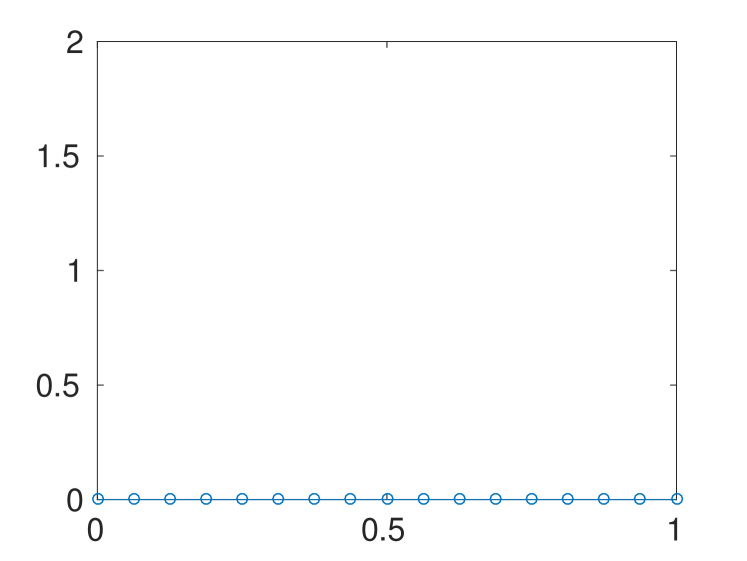
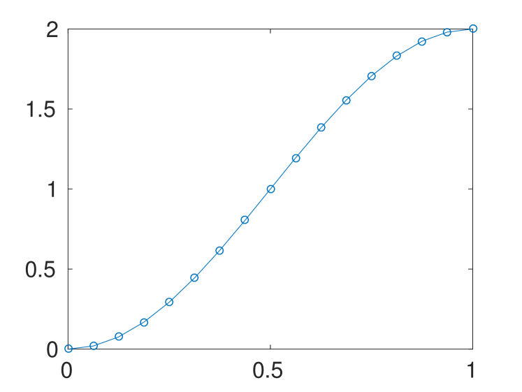
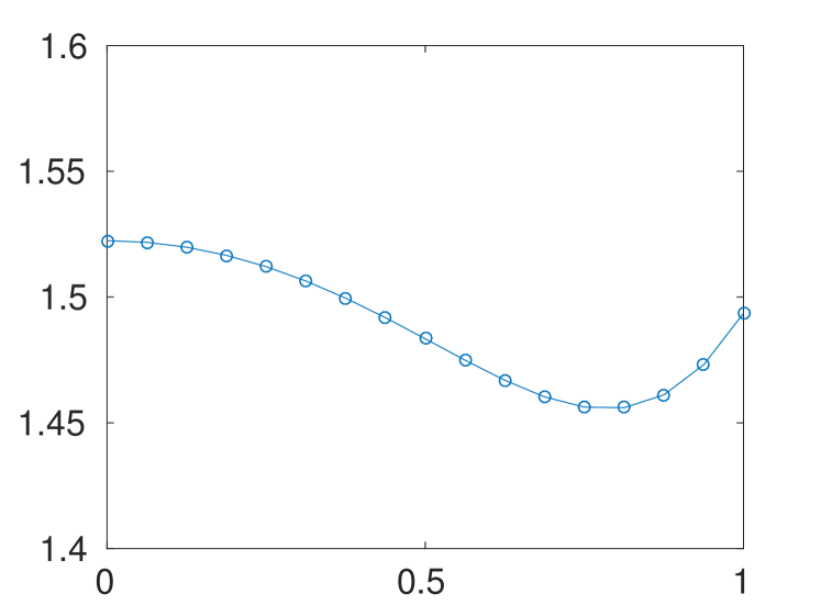
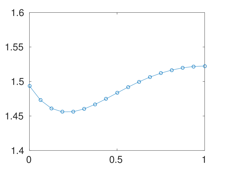
Let us start with verifying the convergence rates obtained in Section 4. To this end, we study the chemotaxis problem on a network consisting of three pipes meeting at a junction; see Figure 2.1. We choose the edge lengths and the parameters , for . For the initial values we let
In the following, we present the time-evolution of the two concentrations with discretization parameters . This setup leads to the occurrence of a peak of both concentrations at vertex . The time-evolution is illustrated in figures 7.1 and 7.2.

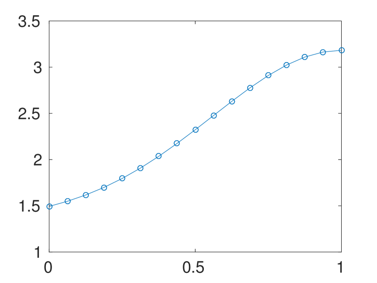
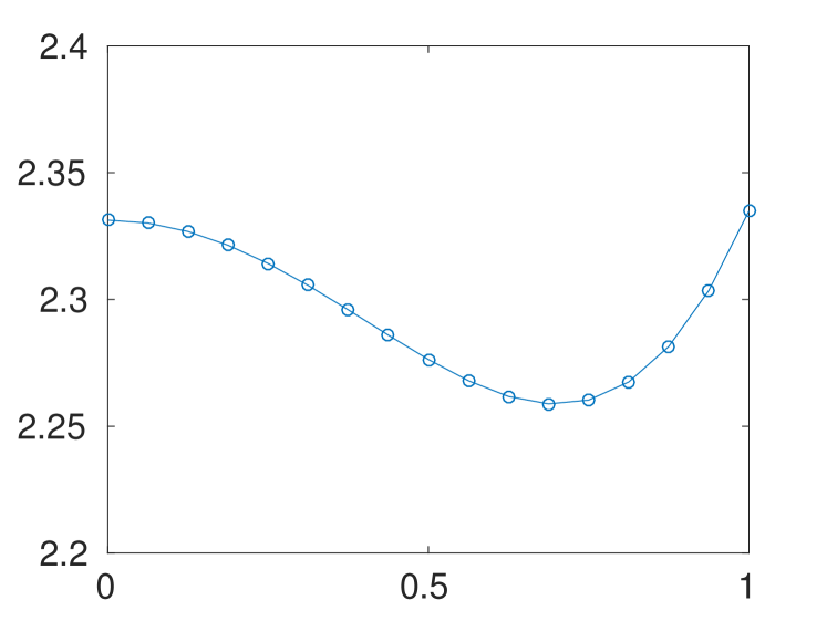
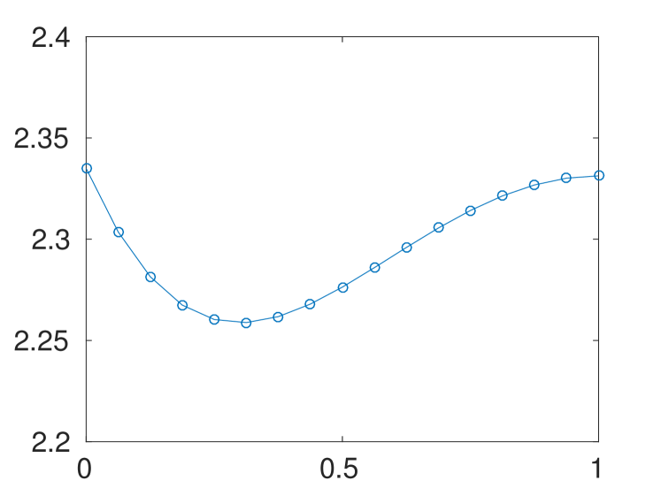
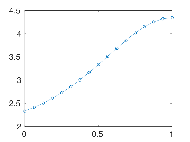
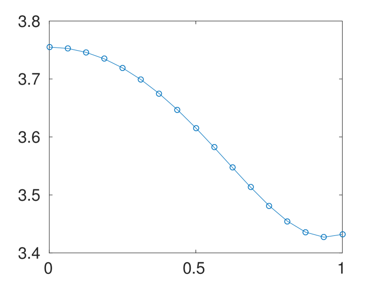
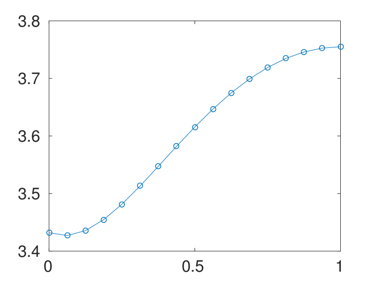
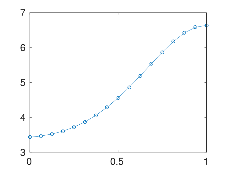
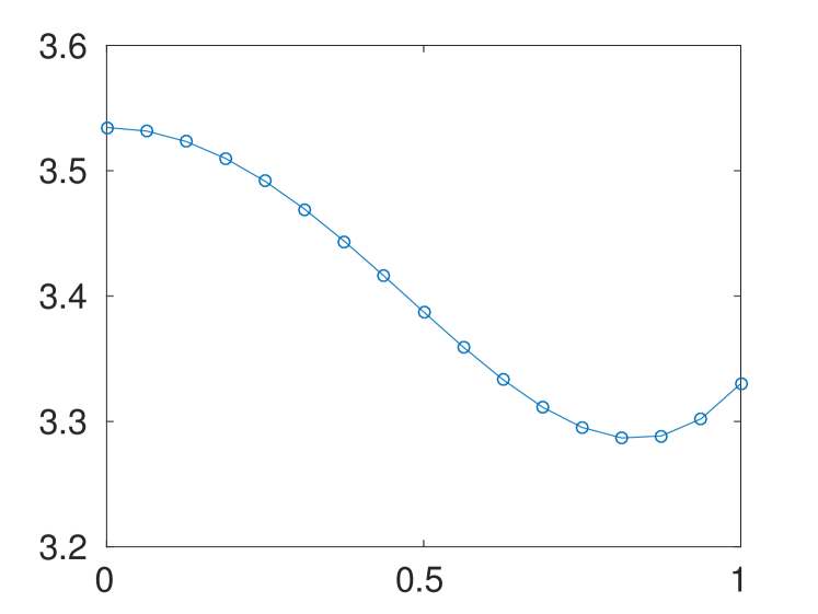
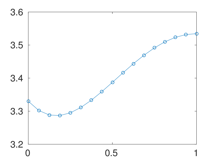
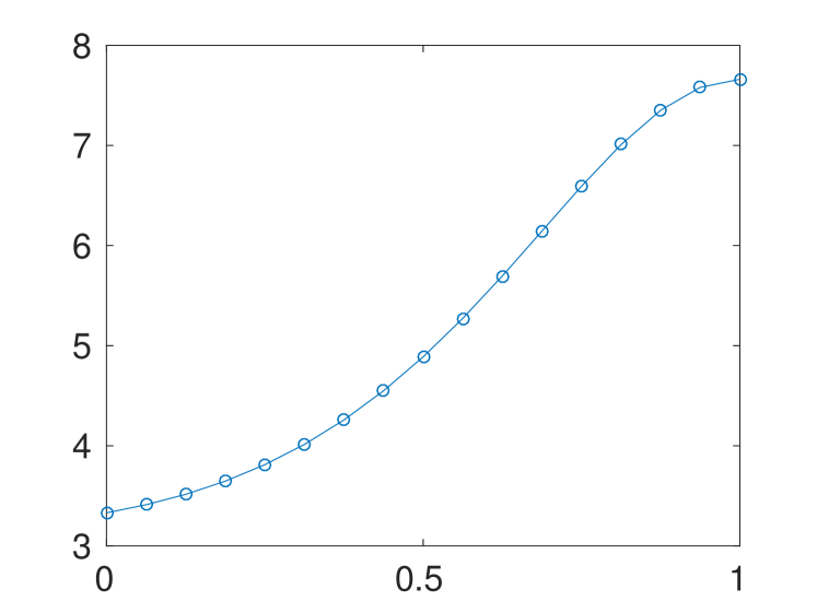
In order to verify the theoretical convergence rates obtained in section 6, we proceed as follows: Since no analytical solution is available for this test case, we use the difference between the numerical solutions on two different meshes with meshsize and as an approximation for the actual error. Since the method has been proven to converge with a given rate, this yields accurate approximations for the true error. The results obtained in our numerical tests are presented in Table 7.1 and 7.2.
| eoc | eoc | ||||
|---|---|---|---|---|---|
| 0.096656 | – | 0.008712 | – | ||
| 0.049195 | 0.97 | 0.004392 | 0.99 | ||
| 0.024821 | 0.99 | 0.002205 | 0.99 | ||
| 0.012467 | 1.00 | 0.001105 | 1.00 | ||
| 0.006248 | 1.00 | 0.000553 | 1.00 |
| eoc | eoc | ||||
|---|---|---|---|---|---|
| 0.027456 | – | 0.002500 | – | ||
| 0.013808 | 0.99 | 0.001252 | 1.00 | ||
| 0.006947 | 0.99 | 0.000627 | 1.00 | ||
| 0.003499 | 0.99 | 0.000313 | 1.00 | ||
| 0.001766 | 0.99 | 0.000156 | 1.00 |
As predicted by our theoretical results in Section 6, we observe first order of convergence in both solution components and norms used for our analysis.
7.2. Block network
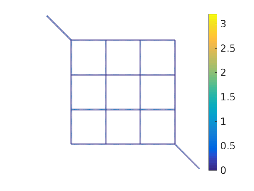
As a second test case, we consider an example proposed in [2], namely the block network depicted in Figure 7.3.
The set of edges is here partitioned into two disjoint subsets
of pipes with different physical properties. The lengths of the pipes are chosen as for all , but the model parameters are chosen differently by
The initial values for the two solution components are simply chosen as
In order to get an interesting behavior, the boundary conditions at the two ports of the network are chose as follows:
This means that the bacteria with density enter the network at node and they are expected to move towards where the chemoattractant is added. Due to the different properties of the individual pipes, we expect the bacteria to move along the red path highlighted in Figure 7.3. Some snapshots of the solution and computed with meshsize and time step are shown in Figures 7.4 and 7.5.
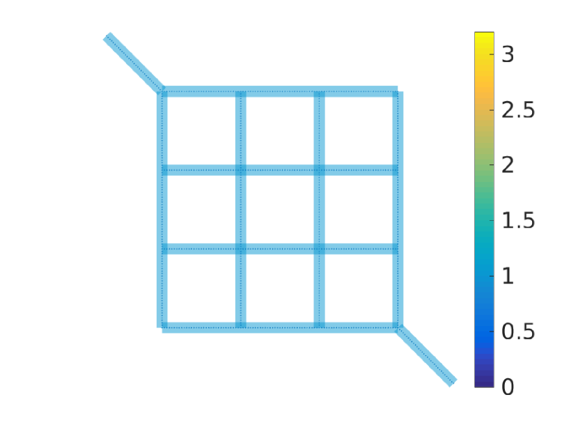
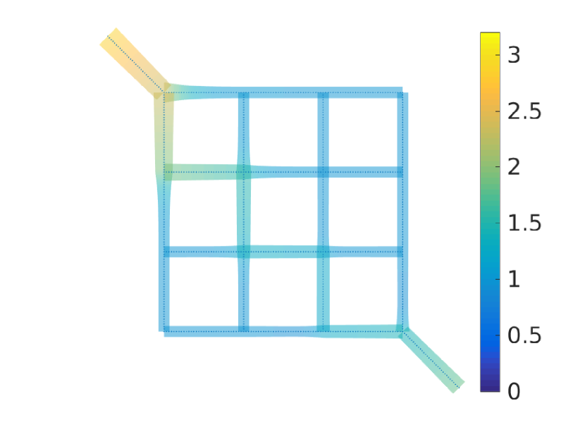
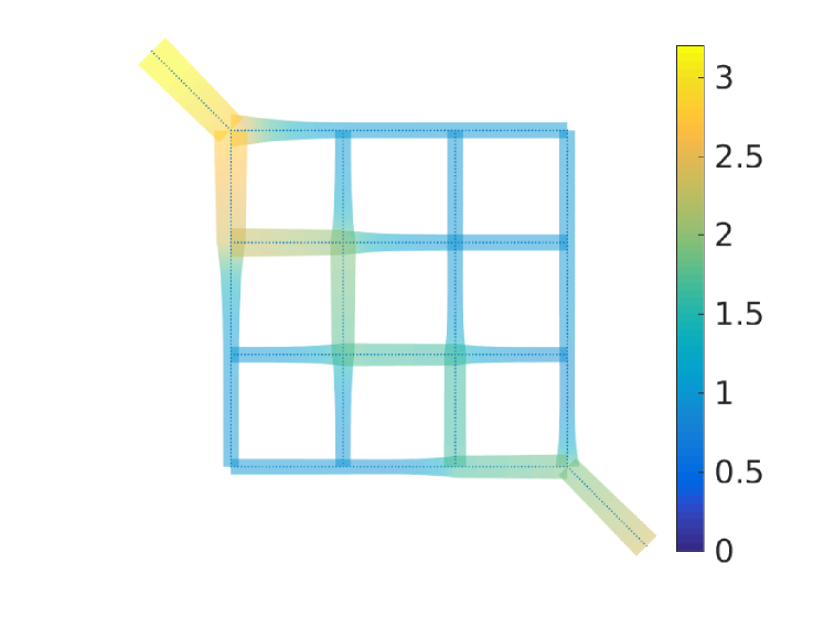
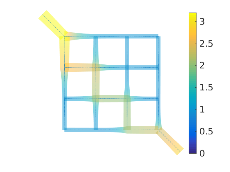
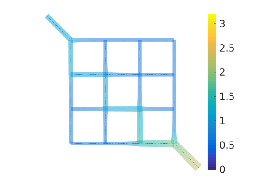
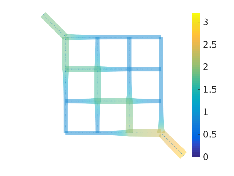
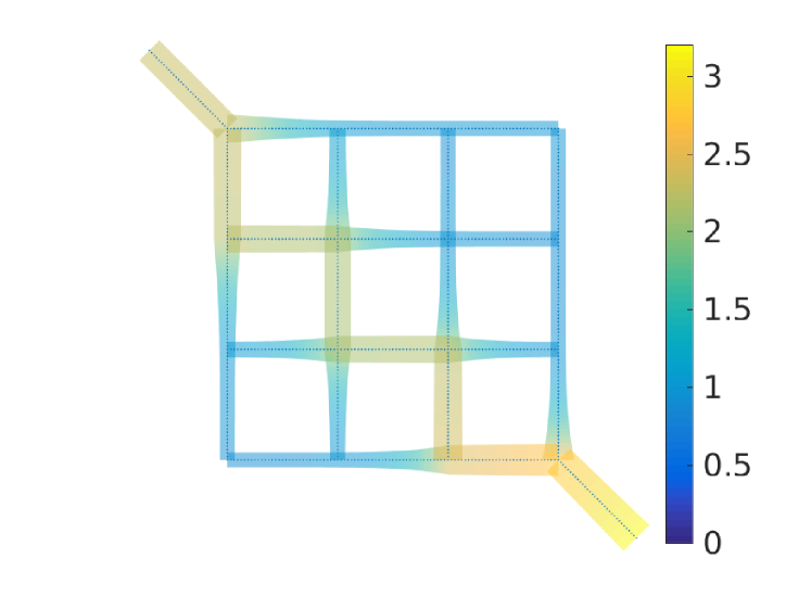
As can be seen from the images, both solution components are smooth and the system behavior seems to be computed correctly as expected.
8. Summary and discussion
In this paper, we considered a chemotaxis model on networks described by a system of partial differential-algebraic equations, which can be seen as a natural generalization of the minimal model to the network context. By extending the results of Osaki and Yagi, we were able to establish global existence and uniqueness of solutions based on perturbation arguments for semilinear evolution problems, conservation of mass, and positivity of the solutions. In addition, we derived regularity estimates for the solutions.
The arguments of the proofs were developed in a way that allowed us to prove the global existence and uniqueness of solutions also for numerical approximations obtained by a finite element discretization with mass lumping and upwinding and an implicit Euler method for time integration. The discrete approximations could be shown to converge to the unique global solution of the chemotaxis problem without artificial smoothness requirements on the solution. In addition, we could establish order optimal convergence rates under minimal smoothness assumptions.
The arguments used for the analysis of the finite element method presented in this paper may be used to improve also the convergence results of the method of Saito [31], in particular, to get rid of the strong stepsize restrictions needed there. Also a generalization to chemotaxis models with nonlinear coefficients seems possible to some extent. A class of problem that would certainly deserve further considerations, also from a numerical point of view, are models of haptotaxis, where no diffusion is present in the equation governing the chemoattractant.
Acknowledgements
The authors are grateful for financial support by the German Research Foundation (DFG) via grants IRTG 1529, TRR 146, and TRR 154 and by the “Excellence Initiative” of the German Federal and State Governments via the Graduate School of Computational Engineering GSC 233 at Technische Universität Darmstadt.
Appendix
In the following sections, we present some auxiliary results that were used in our analysis and we provide complete proofs for some results mentioned in the paper.
Appendix A Auxiliary results
The following embedding inequalities are used several times in our proofs.
Lemma A.1.
Let be a finite metric graph. Then for any ,
| (A.1) | ||||
| (A.2) |
for all with a constant only depending on the geometry of the graph.
Proof.
The assertions follow by applying the classical Gagliardo-Nirenberg inequality on every edge, summation over all edges, using the equivalence of the -norms on finite sequences, and application of Young’s inequality. ∎
We also require the following continuous and discrete version of Gronwall’s inequality.
Lemma A.2 (Gronwall’s lemma, see [12]).
Assume is a nonnegative, absolutely continuous function and are nonnegative, integrable functions on such that
Then
Lemma A.3 (Discrete Gronwall’s lemma, see [17]).
Let and for be nonnegative numbers such that
Further suppose that for and set . Then
| (A.3) |
Appendix B Proof of Theorem 3.1
For convenience of the reader, we now present a complete proof of Theorem 3.1. As a first step, we consider the following linearized variational equations
| (B.1) | |||||
| (B.2) |
where is some given function. In the following lemmas, we summarize the main results about well-posedness of the corresponding initial value problem and derive a-priori estimates for its solutions.
Lemma B.1.
Let (A1) hold and . Then for any and any , there exists a unique weak solution of equation (B.2) with initial value . Moreover, the solution can be bounded by
for a..e with . If , then additionally
with constant depending only on the bounds in (A1).
Proof.
Existence of a unique weak solution follows by Galerkin approximation and standard arguments; see [10, 12] for details. To keep track of the constants, we give a short proof of the a-priori estimates. Testing the variational equation (B.2) with yields
Here we used the bounds for the coefficients for the first step and Young’s inequality with for the second. An application of Lemma A.2 with further yields
The first estimate then follows by noting that , which follows by the Cauchy-Schwarz inequality, and some further elementary computations. For the second bound of the lemma, we test (B.2) with which yields
By rearranging the terms, integration in time, and using assumption (A1), we obtain
This yields the second estimate and completes the proof of the lemma. ∎
As a next step, we now derive a-priori estimates for the second solution component.
Lemma B.2.
Let (A1) hold and . Then for any and , there exists a unique weak solution of (B.1) with initial value . Moreover, the solution can be bounded by
with constant that only depends on the graph, on the bounds in assumption (A1), and on the norm of the data.
Proof.
Testing (B.1) with , we obtain via assumption (A1) that
where we used Lemma A.1 to estimate . Choosing and applying Young’s inequality yields
with a constant . Inserting this expression in the above estimate, rearranging some of the terms, and applying Lemma A.2 further yields
The result then follows by taking the maximum over on both sides. ∎
By combination of the two previous results, we directly obtain the following assertion.
Lemma B.3.
Based on the previous results, we can define a mapping
| (B.3) |
where with norm and where is the first component of the solution of (B.1)–(B.2) with initial values and . By application of Lemma B.3, we can immediately deduce the following result.
Lemma B.4.
For any , , and , the mapping is well defined on . Moreover, for any there exists such that for all , maps into itself.
Proof.
The assertion follows directly from the previous lemmas. ∎
With similar arguments as employed for the proof of the assertions stated in the previous section, we can show that is Lipschitz continuous on .
Lemma B.5.
Let (A1) hold and let , and be given as in Lemma B.4. Then for any , we have
with Lipschitz constant and constants independent of .
Proof.
Let and denote the solutions of (B.1)–(B.2) with the same initial values and but with different data and . Then
for all suitable test functions and . In addition, . With similar arguments as in the proof of Lemma B.1, one can see that
| (B.4) |
Next observe that satisfies and, in addition, there holds
for any suitable test function and a.a. . By choosing and applying some elementary manipulations, one can deduce that
With similar arguments as were used to bound the term in the proof of Lemma B.2, the first term can be further estimated by
with depending on the graph, on the bounds in assumption (A1), on the norms and of the initial values, as well as on and as required. Using Lemma B.2, Lemma A.1, and (B.4), the second term can be estimated by
with depending on the problem data like as required. A combination of these estimates and an application of Lemma A.2 finally yields the result. ∎
Problem (2.1)–(2.6) is equivalent to the fixed-point problem . As a direct consequence of the previous Lemmas, one can see that for all with chosen sufficiently small, maps into itself and is a contraction. Hence, Banach’s fixed-point theorem guarantees the existence of a unique fixed-point with . An application of Lemma B.3 then yields the assertion of the theorem.
Appendix C Proof of Theorem 3.4
By formally differentiating the system (2.1)–(2.2) we obtain
| (C.1) | ||||
| (C.2) |
where and are the derivatives of the solution . Similarly as in the previous section, we will prove existence of local solutions via Banach’s fixed-point theorem. To this end, we consider the following linearized system
| (C.3) | |||
| (C.4) |
for all and with given.
Lemma C.1.
Proof.
It suffices to prove the a-priori estimate. Existence of a unique solution can then be obtained by Galerkin approximation. According to Lemma B.1, we have
for a.a. . Testing (C.3) with we obtain the differential inequality
Integrating between and , using that , applying the interpolation inequality (A.2) and Gronwall’s lemma, we arrive at
The bound of the lemma is then obtained by taking the supremum over on both sides. ∎
Similarly to the previous section, we can now define the fixed-point map
| (C.5) |
where is chosen as before and where denotes the first component of the solution of system (C.3)–(C.4) with given initial values and . By the previous lemma, is well-defined and maps into itself. As a next step, we verify that is a contraction, if is chosen sufficiently small.
Lemma C.2.
Let the assumptions of Lemma C.1 be valid. Then
with Lipschitz constant , where are constants and are polynomials of that only depend on the problem data and the geometry of the graph.
Proof.
Let and be two solutions of (C.3)–(C.4) with the same initial values and , but with different data . With the same arguments as in the proof of Lemma B.5, we obtain
| (C.6) |
Moreover, the difference satisfies and
By choosing , one can then deduce that
Applying the interpolation inequality (A.2), the estimate (C.6), and using the polynomial bounds from Theorem 3.2, we can deduce the assertion of the theorem by integration and an application of Gronwall’s lemma. ∎
Proof of Theorem 3.4
Lemma C.2 shows that is a contraction on for sufficiently small. By Banach’s fixed-point theorem, the system (C.1)–(C.2) thus has a unique local solution. Since the system is linear w.r.t. and we can extend the solution to arbitrary time-intervals via a bootstrap argument. The condition (A3) of Theorem 3.4 guarantees that and . The piecewise -bound of Theorem 3.4 is obtained from the strong form (2.1)–(2.2) of the system and the previous estimates.
References
- [1] C. Berge. Graphs. 2nd rev. North-Holland, Amsterdam, New York, Oxford, 1985.
- [2] R. Borsche, S. Göttlich, A. Klar, and P. Schillen. The scalar Keller-Segel model on networks. Math. Model. Meth. Appl. Sci., 24:221–247, 2014.
- [3] R. Borsche, J. Kall, A. Klar, and T. N. H. Pham. Kinetic and related macroscopic models for chemotaxis on networks. Math. Models Methods Appl. Sci., 26:1219–1242, 2016.
- [4] S. C. Brenner and L. R. Scott. The Mathematical Theory of Finite Element Methods. Springer, 2008.
- [5] G. Bretti, R. Natalini, and M. Ribot. A hyperbolic model of chemotaxis on a network: a numerical study. ESAIM: Math. Model. Numer. Anal., 48:231–258, 2014.
- [6] F. Camilli and L. Corrias. Parabolic models for chemotaxis on weighted networks. J. Math. Pures Appl., 108:459–480, 2017.
- [7] A. Chertock, Y. Epshteyn, H. Hu, and A. Kurganov. High-order positivity-preserving hybrid finite-volume-finite-difference methods for chemotaxis systems. Adv. Comput. Math., 44:327–350, 2017.
- [8] S. Childress and J. K. Percus. Nonlinear aspects of chemotaxis. Math. Biosciences, 56:217–237, 1981.
- [9] P. Clément. Approximation by finite element functions using local regularization. 9:77–84, 1975.
- [10] R. Dautray and J.-L. Lions. Mathematical analysis and numerical methods for science and technology. Vol. 5. Springer-Verlag, Berlin, 1992. Evolution problems. I, With the collaboration of Michel Artola, Michel Cessenat and Hélène Lanchon, Translated from the French by Alan Craig.
- [11] Y. Epshteyn. Discontinuous Galerkin methods for the chemotaxis and haptotaxis models. J. Comput. Appl. Math., 224:168–181, 2009.
- [12] L. Evans. Partial differential equations. American Mathematical Society, 2010.
- [13] F. Filbet. A finite volume scheme for the Patlak-Keller-Segel chemotaxis model. Numer. Math., 104:457–488, 2006.
- [14] L. Gosse. Asymptotic-preserving and well-balanced scheme for the 1D Cattaneo model of chemotaxis movement in both hyperbolic and diffusive regimes. J. Math. Anal. Appl, pages 964–983, 2012.
- [15] M. A. Herrero and J. J. L. Velázquez. A blow-up mechanism for a chemotaxis model. Ann. Scuola Normale Superiore, 24:633–683, 1997.
- [16] H. G. Heuser. Functional analysis. John Wiley & Sons, Ltd., Chichester, 1982. Translated from the German by John Horváth, A Wiley-Interscience Publication.
- [17] J. G. Heywood and R. Rannacher. Finite-element approximation of the nonstationary navier–stokes problem. part iv: Error analysis for second-order time discretization. SIAM J. Numer. Anal., 27:353–384, 1990.
- [18] T. Hillen and K. Painter. Global existence for a parabolic chemotaxis model with the preventiona of overcrowding. Adv. Appl. Math., 26:280–301, 2001.
- [19] T. Hillen and K. J. Painter. A user’s guide to pde models for chemotaxis. J. Math. Biol., 58:183, 2009.
- [20] T. Hillen and A. Potapov. The one-dimensional chemotaxis model: global existence and asymptotic profile. Math. Meth. Appl. Sci., 27:1783–1801, 2004.
- [21] D. Horstmann. From 1970 util present: the Keller-Segel model in chemotaxis and its consequences I. Jahresberichte DMV, 105, 2003.
- [22] W. Jäger and S. Luckhaus. On explosions of solutions to a system of partial differential equations modelling chemotaxis. Trans. Am. Math. Soc., 329:817–824, 1992.
- [23] E. F. Keller and L. A. Segel. Model for chemotaxis. J. Theor. Biology, 30:225–234, 1971.
- [24] D. Mugnolo. Semigroup methods for evolution equations on networks. Springer, 2014.
- [25] T. Nagai, T. Senba, and K. Yoshida. Application of the Moser-Trudinger inequality to a parabolic system of chemotaxis. Funkc. Ekvacioj, 40:411–433, 1997.
- [26] E. Nakaguchi and A. Yagi. Full discrete approximations by Galerkin method for chemotaxis growth model. Nonlin. Anal., 47:6097–6107, 2001.
- [27] R. Natalini and M. Ribot. Asymptotic high order mass-preserving schemes for a hyperbolic model of chemotaxis. SIAM J. Numer. Anal., 50:883–905, 2012.
- [28] K. Osaki and A. Yagi. Finite eimensional attractor for one-dimensional Keller-Segel equations. Funkcialaj Ekvacioj, 44:441–469, 2001.
- [29] R. J. Plemmons. -matrix characterizations. I. Nonsingular -matrices. Linear Algebra and Appl., 18:175–188, 1977.
- [30] T. s. Roubí ček. Nonlinear partial differential equations with applications, volume 153 of International Series of Numerical Mathematics. Birkhäuser/Springer Basel AG, Basel, second edition, 2013.
- [31] N. Saito. Error analysis of a conservative finite-element approximation for the keller-segel system of chemotaxis. Commun. Pure Appl. Anal, 11:339–364, 2012.
- [32] R. Strehl, A. Sokolov, D. Kuzmin, D. Horstmann, and S. Turek. A positivity-preserving finite element method for chemotaxis problems in 3D. J. Comput. Appl. Math., 239:290–303, 2013.
- [33] V. Thomée. Galerkin finite element methods for parabolic problems, volume 25 of Springer Series in Computational Mathematics. Springer-Verlag, Berlin, second edition, 2006.
- [34] R. S. Varga. Functional Analysis and Approximation Theory in Numerical Analysis. CBMS-NSF Regional Conference Series in Applied Mathematics. SIAM, Philadelphia, 1971.
- [35] M. F. Wheeler. A priori error estimates for Galerkin approximations to parabolic partial differential equations. SIAM J. Numer. Anal., 10:723–759, 1973.
- [36] A. Yagi. Norm behavior of solutions to the parabolic model of chemotaxis. Mathematica Japonica, 45:241–265, 1997.