Solitary Waves in a Parabolic Potential: Existence, Stability, and Collisional Dynamics
Abstract
We explore a model with an added external parabolic potential term. This term dramatically alters the spectral properties of the system. We identify single and multiple kink solutions and examine their stability features; importantly, all of the stationary structures turn out to be unstable. We complement these with a dynamical study of the evolution of a single kink in the trap, as well as of the scattering of kink and anti-kink solutions of the model. We see that some of the key characteristics of kink-antikink collisions, such as the critical velocity and the multi-bounce windows, are sensitively dependent on the trap strength parameter, as well as the initial displacement of the kink and antikink.
1 Introduction
Models of the sine-Gordon (sG) ussg and more generally of the nonlinear Klein-Gordon type, such as belova have been studied intensely via a combination of analytical and numerical techniques for well over three decades now. Part of the reason for this widespread appeal concerns the diverse set of physical applications for which such models have been argued to be of relevance. These start from the simplest (coupled torsion pendula, motion of dislocations etc. in the case of the discrete sG braun ) and extend far and wide. Case examples include, but are not limited to structural phase transitions behera ; gufan , domain walls arising in cosmological models vilenkin01 ; anninos , simple polymeric models, as well as models of uniaxial ferroelectrics; see, e.g., Ch. 9 in Vach .
However, there is another source of the fascination, especially from an applied mathematics perspective, in non-integrable models such as . This has to do with their remarkable properties related to the collisional dynamics of kinks and anti-kinks. There, resonant phenomena between translational, internal and extended modes have been identified and and a phenomenological “resonance energy exchange mechanism” campbell has been used to characterize features such as the “multi-bounce windows”, the fractal emergence of such windows, and the universal nature of these phenomena not only in , but also in other models such as the double, and the parametric sG equations campbell ; Campbell1 ; anninos . While recent years have seen both a more rigorous mathematical analysis goodman2 and an experimental realization of a system reminiscent of the effective kink-antikink interactions goodman , there have also been further studies causing a renewed interest in the phenomenological approach and towards posing new questions. For instance, particular variations of the model have been shown numerically to possess multi-bounce windows without possessing internal modes shnir1 . It has also been found that by parametrically deforming the model, one can introduce more internal modes and suppress the two-bounce windows simas . Lastly, the recent work of weigel ; weigel2 has performed a careful bookkeeping of the collective coordinate approaches intended to provide an effective description of the collision events. In so doing, a number of nontrivial problems regarding both computing with such reduced models and the conclusions drawn from them have arisen. Thus, despite its time-honored tradition, the study of kink-antikink collisions in non-integrable models remains a surprisingly active field of investigation to this day gani1 ; danial ; gani2 ; gani3 ; gani4 .
In the present work, we examine a different variant of the problem, considering the scenario where an external potential has been imposed on the field theory. In particular, motivated by the extensive work on atomic Bose-Einstein condensates (BEC), we consider a parabolic trap, which in the latter context emulates the role of a generic magnetic confinement pethick ; stringari ; darkbook . This possibility turns out to alter dramatically the properties of the kink waveforms. In particular, even the single kink turns out to be dynamically unstable in the emerging energy landscape. We examine the case of the single kink and its existence, stability and dynamic properties, as well as that of the kink-antikink state. In the latter, we examine the kink-antikink collisions and attempt to capture them by means of low dimensional collective coordinate models. We highlight both the favorable, as well as the unfavorable traits of these models with respect to their ability to capture the full PDE dynamics and raise some relevant possibilities towards future studies.
2 The Model, Calculational Approach and Ground State
Our starting point for the considerations that follow is the classical equation with an added -dependent trapping term:
| (1) |
where the potential function is given by
| (2) |
is the trap strength constant and typically (in settings related to our motivating example of atomic BECs pethick ; stringari ; darkbook ) assumes values in . However, we mostly restrict our attention to the dynamics for , using for most of the data runs 111Although the BEC example is simply of motivating nature, it turns out that in that setting plays the role of longitudinal to transverse trapping, hence to achieve effective one-dimensionality of the system the condition needs to be enforced. This is what motivates our selection here too.. The case has been well-studied in the past and in its analysis, the perturbation theory and collective coordinate methods have been used anninos ; belova ; campbell ; sugiyama ; weigel . We extend these methods to study our variant bearing a trapping in different parameter regimes.
To explore the properties of Eq. (1) we employ the following numerical scheme. First, we use a fourth-order central difference in space (see e.g. anninos ; roy for this and other similar difference schemes). The resulting system of ordinary differential equations is then evolved in time using fourth-order Runge-Kutta methods, ensuring the accuracy of the conservation of the energy. The average value of the energy is of O(1), while the deviations from the mean are no more than O(). We apply free boundary conditions, although as we shall see below this is generally inconsequential because the field effectively vanishes well before the edge of our computational domain. For all our data runs, a spatial step size of was used. Our computations typically use and a spatial grid running in the interval . For smaller values of , we use a larger interval as necessary to ensure the decay of the wavefunction within the computational domain.
The stationary ground state of the system solves the ordinary differential equation (ODE)
| (3) |
is not known explicitly but in the case , it is well-estimated by the Thomas-Fermi (TF) approximation which neglects the spatial variation of (again motivated by similar considerations in atomic condensates pethick ; stringari ) defined by
| (4) |
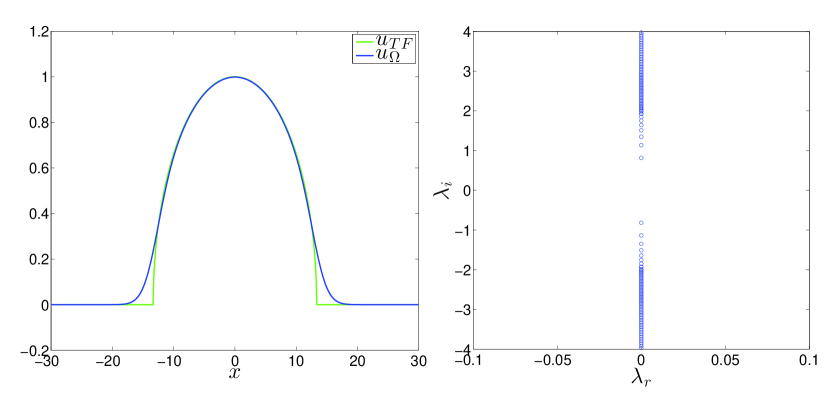
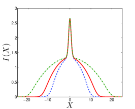
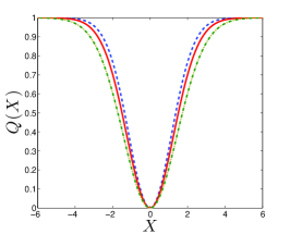
Eq. (4) solves Eq. (3) when the term is neglected. We use this approximation as our initial guess for the Newton-Raphson iterations converging to the true numerical ground state of the system. The comparison of the TF approximation with the true numerical result is given in Fig. 1. At the level of the TF approximation, we note that the ground state is zero whenever , where , which gives
| (5) |
As we can observe in the figure, the TF approximation is very good except for the vicinity of , where its disagreement with the true ground state has been quantified in a series of rigorous studies gallo ; karali .
To study the stability of the ground state, we consider the linearization around the solution using the ansatz:
| (6) |
Here is the numerically obtained ground state, and represent the corresponding eigenvalues and eigenvectors of the linearization. The equation that these satisfy at is of the form:
| (7) |
For the ground state we find, as is shown in the right panel of Fig. (1) that all the eigenvalues lie on the imaginary axis, hence the relevant state is spectrally stable; for instability to arise, at least one of the relevant eigenstates should correspond to growth, i.e., to Re.
3 Single Kink Solutions
We now turn to excited states in the system in the form of kinks and anti-kinks, as well as bound states thereof. We start with the single static kink whose solution is not known explicitly but can be numerically approximated by
| (8) |
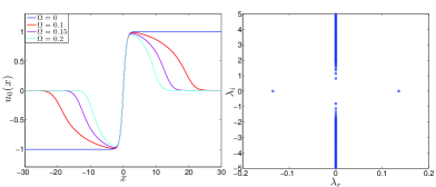
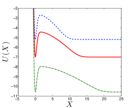
once again in the TF approximation. For various values of , the numerically calculated solutions are shown in Figure 2.
In the figure, also the spectrum of linearization around the single kink is shown (right panel). We see that in all the cases of nonzero , there exists a pair of nonzero real eigenvalues. More concretely, the eigenvalue pair that used to be at due to translational invariance now exists as real and leads to the instability of the kink, which is progressively stronger, the larger the value of .
3.1 Numerical Results (PDE)
We now examine the dynamical evolution of such unstable kinks. As a means of obtaining moving kink solutions (or antikink solutions ) of (1), we can employ the Lorentz transformation, where , where is the initial position and is the velocity of the moving kink. The initial conditions of the PDE are
Of course the model in the presence of the potential is no longer Lorentz invariant (as it is in the case of ). Nevertheless, our results have shown that from a numerical perspective producing a Lorentz-boosted kink and multiplying it by the (stationary) TF background is an efficient method to produce “moving” waveforms starting from standing ones.
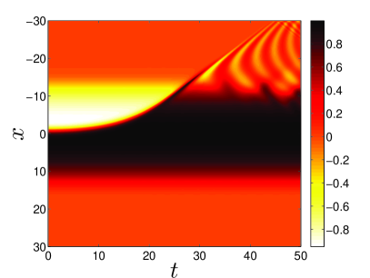
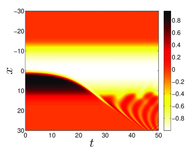
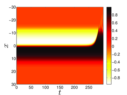
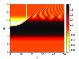
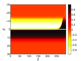
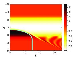
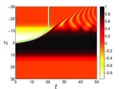
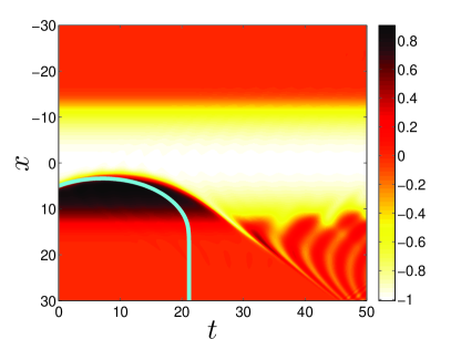
The presence of the the trapping term causes the velocity of the kink not to remain constant (as it would under stationary initialization in the untrapped, translationally invariant problem). When the initial velocity () is zero, the numerical results show that the motion of the kink solution depends sensitively on its starting position. When the kink starts to the left of the origin (), the kink slides to the left, accelerating as it does so. If the kink starts to the right of the origin (), then it slides to the right. In both cases, the kink eventually ends up being expelled from the system. Fig. 3 shows examples of initializing the kink both to the left and to the right of the fixed point at with no speed and illustrates how the kink slides along the side where it starts. This corroborates in a definitive way the results of the stability analysis in that the kink now (in the presence of the parabolic trap) encounters a saddle point at (the center of the trap). Hence, on each side of this unstable equilibrium, it will slide along the unstable manifold. In fact, it is interesting to note that in panel (c) of the figure the kink is initialized at (up to numerical roundoff error). We can see that in that case, it stays at the origin for a long time, until eventually the projection of the roundoff error in the unstable eigendirection grows to O and kicks the kink away from the unstable equilibrium (in the case of this particular example its center moves to , but it can just as well move to the , depending on the perturbation).
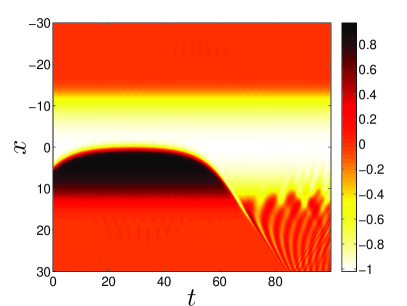
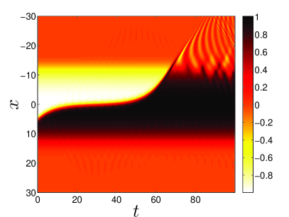
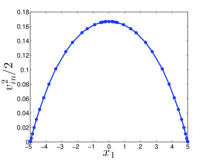
With nonzero initial velocity, the behavior of the kink depends on the magnitude of the velocity. For a kink starting away from the origin, the saddle point at the represents a finite (potential) energy barrier which the kink must overcome to break through to the other side. Given sufficient kinetic energy, a kink moving towards the origin will overcome this potential energy barrier. On the other hand, if the velocity (and hence the kinetic energy of the kink is “subcritical”, i.e., below the value needed to overcome the potential barrier) then the kink will bounce off the barrier and return to be expelled on the side that it started. Fig. 4 (a),(b) demonstrate these two scenarios in a convincing way numerically. In particular, between and of the left and right panel, respectively, there is clearly a critical velocity as the former results in a bounce-back of the kink from , while the latter leads to its transmission through the barrier and on to the other side. For any , the kink stops at , called a turning point and then moves in the opposite direction. The Fig. 4 (c) shows the relation between the effective potential approximated by the associated kinetic energy (per unit mass) and the turning point . Of course, in a way consistent with the above picture, if the kink is initially moving away from the origin, then it will continue to move away and gradually accelerate over time.
3.2 Collective Coordinate Approach (ODE)
In this section we formulate a “collective coordinate” (CC) approach for the dynamics for the single kink. Our aim is to reduce the full PDE with infinitely many degrees of freedom to an ODE model with a single degree of freedom. This is partly driven by previous CC studies of the motion of a kink in the homogeneous case (), including the work of Sugiyama sugiyama (see also anninos ). It is also importantly motivated by the nature of the motion in the vicinity of the saddle point discussed above, and by the desire to obtain a simplified description of this motion.
To begin, we note that the full PDE conserves the energy (Hamiltonian)
| (9) |
where the kinetic and potential energies of the kink, respectively, are
The corresponding Lagrangian is
| (10) | ||||
Assuming that we operate in the TF limit of , we seek to characterize the kink motion by utilizing the ansatz
where is the time-dependent displacement of the kink from the origin and is the ground state of the system in the presence of the trap. Then, the Lagrangian becomes as follows:
where
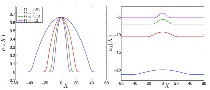
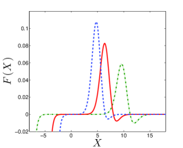
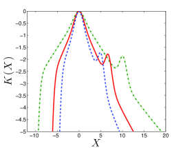
Since we have an extremely accurate numerical solution for , we compute the coefficients and and solve the Euler-Lagrange equation numerically. Fig. 5 shows the plots of and as a function of for various values of . By applying the Euler-Lagrange equation, we obtain the dynamical evolution:
| (11) | ||||
We solve these equations numerically by using the initial conditions and where is the initial position of the kink and is the initial velocity of the kink. We use MATLAB’s built-in fourth-order Runge–Kutta variable-step size solver ode45 with built-in error control. Note that here, overdots denote time derivatives.
Connection to Numerical Results
We now compare our full numerical results (PDE) with the findings of the CC ODE Method. The numerical CC computations show that when the initial velocity is zero (), with nonzero displacement ( or ), the ODE results agree with PDE results quite well up to the time/location when/where the kink is expelled from the system; from there on the kink cannot be clearly discerned anyway, and hence it is not particularly meaningful to seek to track it in the PDE or to match it to the ODE results. Fig. 6(a) and (c) show that when and , with zero initial velocity, both results mostly agree until when the kink is expelled from the TF background.
In the case of zero displacement () and zero velocity () of Fig. 6(b), both the ODE and the PDE show the kink as residing on the saddle point for a long time interval. In the ODE case, the absence of additional degrees of freedom and the conservation of the energy does not allow the kink to depart from the unstable equilibrium over the time horizons considered. In the infinite dimensional system, the instability is manifested at .
When the initial velocity is nonzero, we find similar results. The ODE results agree with the PDE results until the ODE kink is expelled from the system. Fig. 7 (a) exhibits the ODE and PDE agreement until when and . Fig. 7 (b) exhibits this type of agreement until when and . In summary, we can infer that while the kink remains within the region where the TF background is accurate, the CC method appears to yield an excellent qualitative and a very good quantitative characterization of the resulting motion.
4 Kink-Antikink Solutions
Armed with our understanding of the single kink energy landscape, we now turn to case of a kink-antikink pair. Such a state can in fact be stationary in our model, although it is never genuinely stationary in the case of . The reason is fairly similar to the corresponding existence of a stationary state in a nonlinear Schrödinger (NLS) model with a trap analyzed in detail, e.g., in coles . However, there is a crucial difference. In the latter case, the trap has a restoring contribution, while the dark solitons (the kinks) of the NLS repel each other. Here, the situation is reversed: namely, as we saw in the previous section, the trap tends to expel the kink, while (as is known from the study of kink-antikink interactions in the homogeneous case) the kink and antikink attract each other anninos ; campbell , i.e., the role of both contributions is reversed. As a result, the equilibrium point instead of being a center as it is in the case of NLS, here, again, it is a saddle. Indeed, if the kink pair is separated by a small distance, then the interaction prevails and forces the kinks to approach each other. On the other hand, a large separation leads to a dominant effect due to the trap, and the kink-antikink pair are pushed apart.
The static kink-antikink solution of (1) can be numerically approximated by
| (12) |
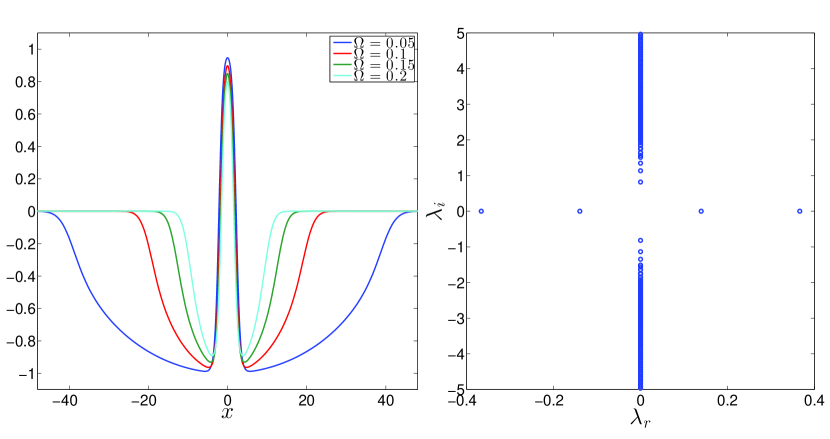
where is unique and dependent on . We define that particular as , since it operates as a critical value separating between expulsion from and attraction of the kink and antikink to the center. For various values of , the numerically calculated stationary kink-antikink solutions are shown in Figure 8. As usual, the right panel of the figure identifies the spectrum of the linearized operator about the static (in this case kink-antikink) solution. Here, we get two pairs of real eigenvalues, indicating instability. The pattern of the spectral problem is thus transparent: for one kink, there is a single unstable mode, for two kinks, two such modes and so on. Another way to state this is that all the negative energy eigenstates of coles pertaining to the normal modes of vibration of the kinks in the real-field version of the model lead to unstable eigendirections.
4.1 Numerical Results (PDE)
We can obtain moving kink-antikink solutions by picking the initial conditions
where , are the initial positions and are the velocities of the moving kink and antikink. Once again, we utilize the (no longer representing an invariance) Lorentz boost and find it to be an efficient method of producing moving kinks-antikinks.
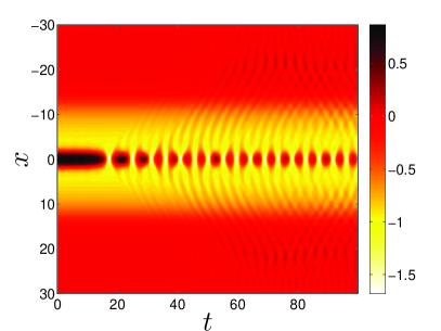
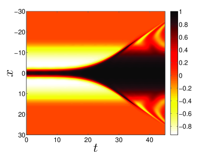
Fig. 9 shows that when the velocity of the kink and antikink is initially zero, then for any (for ), the kink-antikink system forms a bound state. For any , the system exhibits expulsion. This confirms our spectral understanding of the relevant equilibrium representing a saddle point. Now the unstable manifold consists of two eigendirections, namely the in-phase and out-of-phase motion of the pair, although here only the out-of-phase mode is excited.
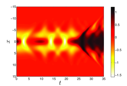
When , the kink-antikink system is relatively insensitive to changes in the initial position (provided that the kinks are not too close). This, however, changes in the presence of the parabolic trapping term. For sufficiently small, the kink and antikink approach each other and collapse into a bound state for small input velocities, even with zero initial velocity. For and initial velocities sufficiently large we observe the typical behaviors that are familiar from the homogeneous case campbell ; anninos : reflection, -bounce windows (i.e., windows where the kinks escape each other’s attraction upon collisions), and “bion/breather” eilbeck ; campbell formation (i.e., emergence of a bound state that oscillates in time and gradually decays). In fact, the types of resonance windows observed in the homogeneous case campbell ; anninos ; goodman2 persist in the inhomogeneous case and present a similar type of pattern. A visualization of this can be seen in Fig. 10. In this figure and in subsequent figures, we opt not to plot velocities for which four or more bounces occur, as the windows become exceedingly narrow for this many bounces and it is not practical to display them together with one- and two-bounce windows. Just as when , the regions in between resonance windows correspond to “bion” formation (numerically these are treated as events with many bounces, so they are omitted from the figures).
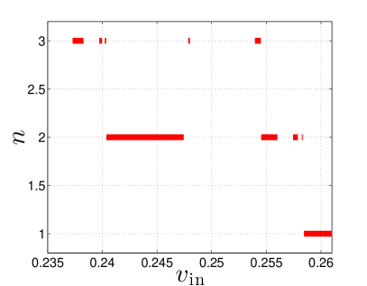
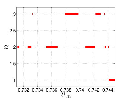
For , the presence of the saddle point of the energy once again imposes a barrier that the kinks need to overcome in order to interact. Thus, in this case, there is a critical velocity associated to , which we denote by , such that whenever and the kinks do not have enough kinetic energy to reach the origin, so they stop (at a turning point) before they reach it. Then they recede towards spatial infinity without ever having collided.
If both and , then the kinks will have enough kinetic energy to overcome the barrier, reach the origin and collide, and then we observe the typical phenomena associated with the model, including most notably the existence of multi-bounce windows. These can be visualized in Figs. 10 and 16 with both small and large separation , respectively. The velocity interval data that was used to create these figures is contained in Tables 1–4 in Appendix A.
4.2 Collective Coordinate Approach (ODE)
To complement our PDE simulations, we formulate a collective coordinate model for a kink-antikink configuration. As before, our aim is to reduce the full PDE with infinitely many degrees of freedom to a simple model with two degrees of freedom in a way similar to what has been previously done in the homogeneous case campbell ; anninos ; goodman2 ; goodman . To account for the internal modes of the kink and antikink, we introduce a new unknown , representing the amplitude of the internal mode. We use only one function for both modes since the collision picture is symmetric between kink and antikink, so we expect the amplitudes of the kink mode and antikink mode to coincide if the initial configuration is symmetric. Our corresponding ansatz in this case will be:
| (13) |
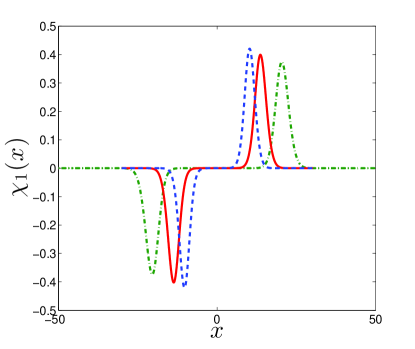
where , and is an eigenfunction corresponding to the smallest positive eigenfrequency that satisfies the linearization equation for a single kink.
The particular eigenfunction we chose is given in Figure 11 for three different values.
Surprisingly, these modes are related chiefly to the background state rather than to the internal vibrational mode of the kink. More specifically, they are localized near . In the homogenous model, the only nonzero discrete eigenfrequency corresponds to the internal vibrational mode, and it is this mode that is used for the collective coordinate ansatz. For our model, the mode with the smallest eigenfrequency results in a better match of collective coordinate and PDE results than when the (analogue of the homogeneous case kink) internal mode is used. This may be due to the former mode incorporating more adequately the role of the potential-induced background, although, admittedly, this issue warrants further theoretical investigation.
As proposed in sugiyama , we work on a reduced effective Lagrangian that captures the fundamental features. The derivations of the formulas are in Appendix B.
| (14) |
Figs. 12 and 13 show the collective coordinate coefficients as functions of for various values of .
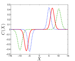
The Euler-Lagrange equations in this case with respect to and give
| (15) | ||||
Here, overdots denote time derivatives. We solve these equations numerically by using the initial conditions , , and where is the initial half-distance between the kink and the antikink, and is the initially prescribed speed of the kink (and anti-kink). Note that this is the reduced system where the higher order terms of and are ignored. We make this assumption based on the previous work sugiyama , that higher terms of and can be dropped because they are small. The expressions involving integrals which are -dependent in Eqs. (15) are computed by numerical integration.
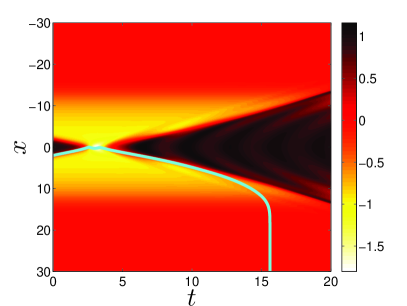
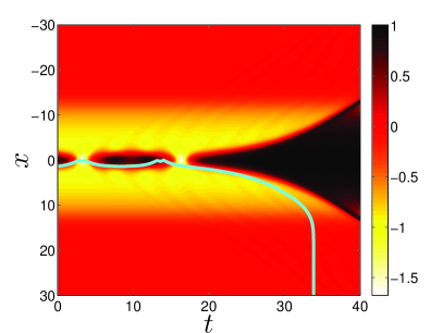
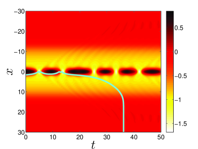
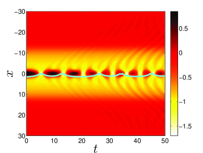
For values not much larger than the value considered so far (of ), the phenomenology is virtually identical to that of the previous section. All of the interactions we have come across so far, namely bions, multi-bounce interactions, and expulsion, are observed for kink-antikink systems as the initial velocity is varied. Figure 16 shows the presence of two- and three-bounce windows and a threshold reflection velocity for and . However, the widths of existing bounce windows shrink drastically as the trap strength is increased. Increasing from to as in the same figure shrinks the resonance windows by approximately a factor of . Our collective coordinate model also exhibits these features – it is capable of capturing one- and two-bounce interactions, and exhibits the same sensitive dependence on the initial speed we observe when is small for configurations with more bounces. Examples can be seen in Figure 17.
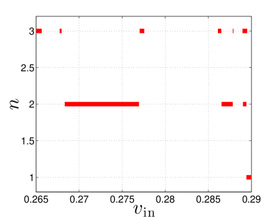
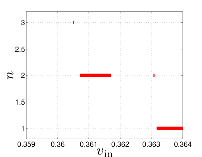
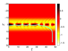
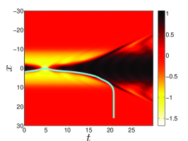
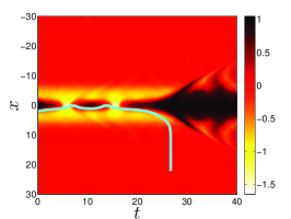
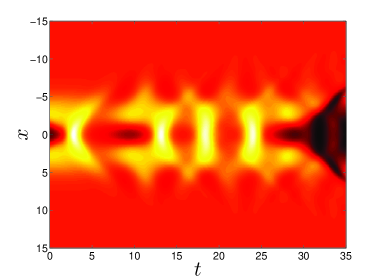
Thus far we have confined ourselves to the case . However, the behaviors for larger are interesting in their own right and can differ significantly from those observed for weak trapping. Intuitively, we expect that a large value of will constrain the dynamics severely (as it only allows the kinks to move within a restricted TF region). Our numerical simulations suggest that two-bounce and three-bounce still exist there, yet they are extremely narrow and shrink rapidly as increases. Figure 18 shows some prototypical examples of multi-bounce cases for .
5 Conclusions and Future Challenges
In this work we have taken the well-known model in a novel direction: motivated by considerations in atomic BECs where a complex variant of the model is examined in the presence of an external potential, we have explored how the standard phenomenology is affected by a parabolic trapping. We have found that the results can be fundamentally different in comparison to the standard homogeneous (untrapped) case. In particular, even the single kink state is dynamically unstable, representing a saddle point in configuration space and leading to the expulsion of the kink from the trap center of symmetry. Moreover, in the presence of multiple kinks and anti-kinks, the number of coherent structures determines the number of unstable eigendirections (and the dimension of the corresponding unstable manifold). It is interesting to also observe the reverse role of the potential and of the kink-antikink interaction in comparison with the atomic BEC case. These features generally favor the expulsion of the kinks from the system unless the kinks are sufficiently close to each other that their interaction dominates. In that setting, -bounce windows may still be present, although these windows were found to shrink radically as the potential parameter is increased. Lastly, we have developed a collective coordinate low-dimensional ODE approach, under relevant approximations (such as the truncation of the higher power terms) which yields, especially for low numbers of bounces, reasonably consonant results between the PDE field theory and the ODEs. On the other hand, when presenting a more “complete” variant of the equations, issues similar to those encountered by weigel ; weigel2 in the homogeneous variant of the model emerge. Indeed, the prospect of resolving these collective coordinate issues and improving the ODE models in this inhomogeneous variant (and even for the homogeneous case within the model) is an important avenue for possible future work.
From a mathematical standpoint, understanding better the stability properties of the model (e.g. proving rigorously the eigenvalue estimate in the case of kinks, as likely possessing unstable eigendirections) could be an interesting direction for further work. Also, extending inhomogeneous model considerations to other models of recent interest such as the shnir1 ; weigel ; gani1 ; danial ; usrecent , and models gani4 ; gani5 ; ivanrecent would be valuable in understanding the genericity (or not) of the conclusions drawn in this study. Some of these directions are currently under consideration and will be reported in future publications.
6 Tables for bounce windows
We list the velocity intervals that result in multi-bounce windows when the initial velocity is picked within these intervals. In Tables 1–2, we list those intervals for a small separation () and a big separation () with . In Tables 3–4, we list those intervals for bigger values of ( and respectively) with fixed .
| 3 | 0.23729 | 0.23827 | 0.00098 |
|---|---|---|---|
| 3 | 0.23973 | 0.23996 | 0.00023 |
| 3 | 0.24023 | 0.24035 | 0.00012 |
| 2 | 0.24038 | 0.24744 | 0.00706 |
| 3 | 0.24786 | 0.24801 | 0.00015 |
| 3 | 0.25396 | 0.2545 | 0.00054 |
| 2 | 0.25453 | 0.25601 | 0.00148 |
| 2 | 0.25754 | 0.25787 | 0.00033 |
| 2 | 0.25824 | 0.25831 | 0.00007 |
| 2 | 0.2584 | 0.25841 | 0.00001 |
| 2 | 0.73116 | 0.7314 | 0.00024 |
|---|---|---|---|
| 2 | 0.73260 | 0.7331 | 0.00050 |
| 3 | 0.73327 | 0.73331 | 0.00004 |
| 2 | 0.73527 | 0.73686 | 0.00159 |
| 3 | 0.73791 | 0.73981 | 0.0019 |
| 2 | 0.74083 | 0.74214 | 0.00131 |
| 3 | 0.74226 | 0.74228 | 0.00002 |
| 3 | 0.74346 | 0.74353 | 0.00007 |
| 2 | 0.74355 | 0.74376 | 0.00021 |
| 2 | 0.74401 | 0.74411 | 0.0001 |
| 3 | 0.26501 | 0.26565 | 0.00064 |
|---|---|---|---|
| 3 | 0.26775 | 0.26796 | 0.00021 |
| 2 | 0.26833 | 0.27694 | 0.00861 |
| 3 | 0.27703 | 0.27756 | 0.00053 |
| 3 | 0.28611 | 0.28649 | 0.00038 |
| 2 | 0.28654 | 0.28783 | 0.00129 |
| 3 | 0.28784 | 0.2879 | 0.00006 |
| 3 | 0.28896 | 0.28897 | 0.00001 |
| 2 | 0.28902 | 0.28941 | 0.00039 |
| 3 | 0.3605 | 0.36054 | 0.00004 |
|---|---|---|---|
| 2 | 0.36073 | 0.36171 | 0.00098 |
| 2 | 0.36307 | 0.3631 | 0.00003 |
7 Derivation of the coefficients in Eq. (14)
We define and , and . Then Eq. (13) becomes
| (16) |
Substituting (16) into Eq. (10) gives
| (17) | ||||
To handle the terms we first write where and . Then using the Taylor series expansion, we get
| (18) | ||||
The corresponding reduced Lagrangian (ignoring higher order terms) that is used in our simulations is given by Eq. (14). Applying Euler-Lagrange equations, we obtain Eq. (15).
We will list the formulae of the coefficients below. Note that they are all functions of . Since is not known explicitly, the coefficients presented are in the integral form. These coefficients are calculated numerically.
References
- (1) N. Manton, P. Sutcliffe, Topological Solitons, Cambridge University Press (Cambridge, 2004).
- (2) D.K. Campbell, J.F. Schonfeld, and C.A. Wingate, Physica 9D, 1 (1983).
- (3) T. Sugiyama, Prog. Theor. Phys. 61, 1550 (1979).
- (4) J. Cuevas-Maraver, P.G. Kevrekidis, F. Williams, The sine-Gordon Model and its Applications, Springer-Verlag (Heidelberg, 2014).
- (5) T.I. Belova and A.E. Kudryavtsev, Phys. Usp. 40, 359 (1997).
- (6) O.M. Braun, Yu. Kivshar, The Frenkel-Kontorova Model, Concepts, Methods and Applications, Springer-Verlag (Berlin, 2010).
- (7) S.N. Behera and A. Khare, Pramana (J. of Phys.) 15, 245 (1980).
- (8) Y.M. Gufan, Structural Phase Transitions [in Russian], Nauka (Moscow, 1982).
- (9) A. Vilenkin and E.P.S. Shellard, Cosmic Strings and Other Topological Defects, Cambridge University Press (Cambridge, 2000).
- (10) P. Anninos, S. Oliveira, and R.A. Matzner, Phys. Rev. D 44, 1147 (1991).
- (11) T. Vachaspati, Kinks and Domain Walls: An Introduction to Classical and Quantum Solitons, Cambridge University Press (Cambridge, 2006).
- (12) D.K. Campbell and M. Peyrard, Physica D 18, 47 (1986); ibid. 19, 165 (1986).
- (13) R.H. Goodman and R. Haberman, SIAM J. Appl. Dyn. Sys. 4, 1195 (2005).
- (14) R.H. Goodman, A. Rahman, M.J. Bellanich, ane C.N. Morrison, Chaos 25, 043109 (2015).
- (15) P. Dorey, K. Mersh, T. Romanczukiewicz, and Y. Shnir, Phys. Rev. Lett. 107, 091602 (2011).
- (16) F.C. Simas, A.R. Gomes, K.Z. Nobrega and J.C.R.E. Oliveira, JHEP 09, 104 (2016).
- (17) H. Weigel, J. Phys. Conf. Ser. 482, 012045 (2014).
- (18) I. Takyi and H. Weigel, Phys. Rev. D 94, 085008 (2016).
- (19) V.A. Gani, A.E. Kudryavtsev, and M.A. Lizunova, Phys. Rev. D 89, 125009 (2014).
- (20) A.M. Marjaneh, V.A. Gani, D. Saadatmand, S.V. Dmitriev, and K. Javidan, JHEP 2017, 28 (2017).
- (21) V.A. Gani, A.E. Kudryavtsev, M.A. Lizunova Phys. Rev. D 89, 125009 (2014).
- (22) A.M. Marjaneh, V.A. Gani, D. Saadatmand, S.V. Dmitriev, K. Javidan, JHEP 07, 028 (2017).
- (23) E. Belendryasova, V.A. Gani, arXiv:1708.00403.
- (24) C. J. Pethick and H. Smith, Bose-Einstein condensation in dilute gases (Cambridge University Press, Cambridge, 2002).
- (25) L. P. Pitaevskii and S. Stringari, Bose-Einstein Condensation, Oxford University Press (Oxford, 2003).
- (26) J. Dorignac, J.C. Eilbeck, M. Salerno, and A.C. Scott, Phys. Rev. Lett. 93, 025504 (2004).
- (27) D. J. Frantzeskakis, and R. Carretero-González, The Defocusing Nonlinear Schrödinger Equation, SIAM (Philadelphia, 2015).
- (28) I. Roy, S.V. Dmitriev, P.G. Kevrekidis, A. Saxena, Phys. Rev. E 76, 026601 (2007).
- (29) C. Gallo, D. Pelinovsky, Asympt. Anal. 73, 53 (2011).
- (30) G. Karali, C. Sourdis, Arch. Rat. Mech. Anal. 217, 439 (2015).
- (31) M.P. Coles, D.E. Pelinovsky, P.G. Kevrekidis, Nonlinearity 23, 1753 (2010).
- (32) A. Demirkaya, R. Decker, P. G. Kevrekidis, I. C. Christov, A. Saxena, JHEP 2017(12), 71 (2017).
- (33) R.V. Radomskiy, E.V. Mrozovskaya, V.A. Gani, I.C. Christov J. Phys.: Conf. Ser. 798, 012087 (2017)
- (34) A. Khare, I.C. Christov, and A. Saxena Phys. Rev. E 90, 023208 (2014).