A semi-Lagrangian scheme for Hamilton-Jacobi equations on networks with application to traffic flow models.

Abstract

We present a semi-Lagrangian scheme for the approximation of a class of Hamilton-Jacobi-Bellman equations on networks. The scheme is explicit and stable under some technical conditions. We prove a convergence theorem and some error estimates. Additionally, the theoretical results are validated by numerical tests. Finally, we apply the scheme to simulate traffic flows modeling problems.

1 Introduction

The attention to the study of linear and nonlinear partial differential equations on networks raised consistently in the last decades motivated by the extensive use of systems like roads, pipelines, and electronic and information networks.

In particular, extensive literature has been developed for vehicular traffic systems modeled through conservation laws. Existence results can be found in garavello2006traffic , and some partial uniqueness results (for a limited number of intersecting roads) in garavello2007conservation ; andreianov2011theory . Nonetheless, the lack of uniqueness on the junction point obliges to add some additional conditions that may be ambiguous or difficult to derive. More recently, another kinds of macroscopic models appears. These models rely on the Moskowitz function and make appear an Hamilton-Jacobi equation (see newell ).

The theory of Hamilton-Jacobi (HJ) equations on networks is very recent. It is difficult to extend the classic framework to the network context because these equations do not have in general regular solutions and the notion of weak solution (viscosity solution) must be adapted to preserve some properties on the junction points. An additional difficulty comes from possible discontinuities on data of the problem. Some theoretical results are contained in the early works achdou2013hamilton ; camilli2018flame ; imbert2013flux ; imbert2013hamilton ; schieborn2013viscosity where, using some appropriate definitions of weak solutions, the authors prove the well-posedness of the problem. We also refer to the works barles2016flux ; LionsSouganidis for simplified proof of uniqueness. Concerning numerical schemes for this kind of equations, there is very few theoretical results. Let us mention the finite differences scheme proposed in camilli2018flame ; costeseque2015convergent and the paper imbert2015error in which they prove some error estimates for this scheme.

In this paper, we adopt the notion of solutions as introduced in imbert2013flux , which has some good advantages in term of generality, and we introduce a new numerical scheme for HJ equations on a network. For the sake of simplicity, we consider a simplified network (a junction), but the result can be extended to a more general class of problems, including more complex structures.

We propose a semi-Lagrangian (SL) scheme by discretizing the dynamic programming principle presented in imbert2013flux . This scheme generalizes what introduced in camilli2013approximation , and it enables discrete characteristics to cross the junctions. This property makes the scheme absolutely stable, allowing large time steps, and it is the main advantage compared to finite differences and finite elements schemes. We prove consistency and monotonicity which imply the convergence of the scheme.

We also derive some consistency errors for the numerical solution that we can obtain in two different cases: for state independent Hamiltonians, where controls are constant along the arcs, and in a more general scenario. In the simplified case, we obtain a first order convergence estimate. In the second case, the key result is a consistency estimate that leads to an a priori error estimate. The proof is obtained combining some techniques derived from the papers on regional optimal control problems barles2013bellman ; barles2016flux .

Structure of the paper:

in Section 2 we recall some basic notions for junction networks, the definition of flux-limited viscosity solutions and the relation with optimal control problems on networks. In Section 3, we derive the SL scheme and prove its basic properties: consistency, monotonicity, and convergence. In Section 4, we present the main result (Theorem 4.2) concerning the error estimate. In Section 5, we discuss the connection between HJ equations and traffic flow model. Finally, in Section 6, we show through numerical simulations the efficiency and the accuracy of our new method.

2 Hamilton-Jacobi equations on networks

A network is a domain composed of a finite number of nodes connected by a finite number of edges. To simplify the description of such system we focus on the case of a junction, which is a network composed of one node and a finite number of edges. We follow imbert2013flux and the notations therein to describe the problem.
Given a positive number $N$, a junction $J$ is a network of $N$ half lines $J_{i}:=\{k\,e_{i},k\in{\mathbb{R}}^{+}\}$ (where each line is isometric to $[0,+\infty)$ and $e_{i}$ is a unitary vector centered in $0$) connected in a junction point that we conventionally place at the origin. We then have

$$J:=\bigcup_{i=1,...,N}J_{i},\quad J_{i}\cap J_{j}=\{0\},\quad\forall i\neq j,\quad i,j\in\{1,...,N\}.$$

Figure 1: Junction with $N=5$ edges.

We consider the geodesic distance function on $J$ given by

$$d(x,y)=\left\{\begin{array}[]{lll}|x-y|,&&\hbox{if $x,y\in J_{i}$ for one $i\in\{1,...,N\}$},\\ |x|+|y|,&&\hbox{otherwise.}\end{array}\right.$$

For a real-valued function $u$ defined on $J$, $\partial_{i}u(x)$ denotes the (spatial) derivative of $u$ at $x\in J_{i}$ and the gradient of $u$ is defined as:

$$u_{x}:=\left\{\begin{array}[]{lll}\partial_{i}u(x)&&\hbox{if }x\in J_{i}\setminus\{0\},\\ \left(\partial_{1}u(x),\partial_{2}u(x),...,\partial_{N}u(x)\right)&&\hbox{if }x=0.\end{array}\right.$$ (1)

We can now describe our problem. Consider the following evolutive HJ equation on the network $J$

$$\left\{\begin{array}[]{ll}\partial_{t}u(t,x)+H_{i}(x,u_{x}(t,x))=0&\hbox{ in }(0,T)\times J_{i}\setminus\{0\},\\ \partial_{t}u(t,x)+F_{A}(u_{x}(t,x))=0&\hbox{ in }(0,T)\times\{0\},\end{array}\right.$$ (2)

with the initial condition

$$u(0,x)=u_{0}(x)\quad\hbox{ for }x\in J,$$ (3)

where $u_{0}(x)$ is globally Lipschitz continuous on $J$. We suppose that standard assumptions on the Hamiltonian $H$ (cf. i.e. BardiCapuz@incollection ) hold:

• (Regularity) for all $L>0$ there exists a modulus of continuity $\omega_{L}$ such that for all $|p|,|q|\leq L$ and $x\in J_{i}$

  $$|H_{i}(x,p)-H_{i}(x,q)|\leq\omega_{L}(|p-q|);$$

  in addition, $H(\cdot,p)$ is Lipschitz continuous w.r.t. the space variable.

• (Uniform coercivity) $H_{i}(x,p)\rightarrow+\infty$ for $|p|\rightarrow+\infty$ uniformly for every $x\in J_{i}\cup\{+\infty\}$, $i=1,...,N$;

• (Convexity) $\{H_{i}(x,\cdot)\leq\lambda\}$ is convex for every choice of $\lambda\in{\mathbb{R}}$ and a fixed $x\in J$.

Using the convexity hypothesis and the coercivity, there exists a $\hat{p}_{i}$ such that the Hamiltonian $H_{i}$ is non-increasing in $(-\infty,\hat{p}_{i}]$ and non-decreasing in $[\hat{p}_{i},\infty)$. We introduce the (respectively) non-increasing and non-decreasing functions

$$H^{-}_{i}(x,p):=\left\{\begin{array}[]{ll}H_{i}(x,p)&\hbox{for }p\leq\hat{p}_{i}\\ H_{i}(x,\hat{p}_{i})&\hbox{for }p>\hat{p}_{i}\end{array}\right.\hbox{ and }H^{+}_{i}(x,p):=\left\{\begin{array}[]{ll}H_{i}(x,p)&\hbox{for }p\geq\hat{p}_{i}\\ H_{i}(x,\hat{p}_{i})&\hbox{for }p<\hat{p}_{i}.\end{array}\right.$$

Given a parameter $A\in{\mathbb{R}}\cup\{-\infty\}$ (flux limiter), we define the operator $F_{A}:{\mathbb{R}}^{N}\rightarrow{\mathbb{R}}$ on the junction point as

$$F_{A}(p):=\max\left(A,\max_{i=1,...,N}H^{-}_{i}(0,p_{i})\right).$$ (4)

In order to introduce the notion of viscosity solution, we introduce the class of test functions. For $T>0$, set $J_{T}=(0,T)\times J$. We define the class of test functions on $J_{T}$ and on $J$ as

$$C^{k}(J_{T})=\{\varphi\in C(J_{T}),\,\forall i=1,\dots,N,\,\varphi\in C^{k}((0,T)\times J_{i})\},$$

$$C^{k}(J)=\{\varphi\in C(J),\,\forall i=1,\dots,N,\,\varphi\in C^{k}(J_{i})\}.$$

We recall also the definition of upper and lower semi-continuous envelopes $u^{*}$ and $u_{*}$ of a (locally bounded) function $u$ defined on $[0,T)\times J$,

$$u^{*}(t,x)=\limsup_{(s,y)\rightarrow(t,x)}u(s,y)\quad\hbox{ and }\quad u_{*}(t,x)=\liminf_{(s,y)\rightarrow(t,x)}u(s,y).$$

We say that a test function $\varphi$ touches a function $u$ from below (respectively from above) at $(t,x)$ if $u-\varphi$ reaches a minimum (respectively maximum) at $(t,x)$ in a neighborhood of it.

Definition 1 (Flux-limited solutions)

Assume that the Hamiltonians satisfy (H1)-(H3) and let $u:[0,T)\times J\rightarrow{\mathbb{R}}$.

• We say that $u$ is a flux-limited sub-solution (resp. flux-limited super-solution) of (2) in $(0,T)\times J$ if for all test function $\varphi\in C^{1}(J_{T})$ touching $u^{*}$ from above (resp. $u_{*}$ from below) at $(t_{0},x_{0})\in J_{T}$, we have

  $$\begin{array}[]{lll}\varphi_{t}(t_{0},x_{0})+H_{i}(x_{0},\varphi_{x}(t_{0},x_{0}))\leq 0&\quad\hbox{ (resp. $\geq 0$) }&\hbox{ if $x_{0}\in J_{i}$},\\ \varphi_{t}(t_{0},x_{0})+F_{A}(\varphi_{x}(t_{0},x_{0}))\leq 0&\quad\hbox{ (resp. $\geq 0$)}&\hbox{ if $x_{0}=0$}.\end{array}$$ (5)

• We say that $u$ is a flux-limited sub-solution (resp. flux-limited super-solution) of (2) on $[0,T)\times J$ if additionally

  $$u^{*}(0,x)\leq u_{0}(x)\quad{\hbox{(resp. }}u_{*}(0,x)\geq u_{0}(x)){\hbox{ for all}}\;x\in J.$$ (6)

• We say that $u$ is a flux-limited solution if $u$ is both a flux-limited sub-solution and a flux-limited super-solution.

Thanks to the work of Imbert and Monneau imbert2013flux , we have the following result which gives an equivalent definition of viscosity solutions for (2). We use this equivalent definition in particular in the definition of the consistency in Section 3.

Theorem 2.1 (Equivalent definition for sub/super-solutions)

Let $\bar{H}^{0}=\max_{j}\min_{p}H_{j}(p)$ and consider $A\in[\bar{H}^{0},+\infty)$. Given solutions $p_{i}^{A}\in\mathbb{R}$ of

$${H}_{i}\left(p_{i}^{A}\right)={H}^{+}\left(p_{i}^{A}\right)=A$$ (7)

let us fix any time independent test function $\phi^{0}(x)$ satisfying, for $i=1,\dots,N$,

$$\partial_{i}\phi^{0}(0)=p_{i}^{A}.$$

Given a function $u:(0,T)\times J\rightarrow\mathbb{R}$, the following properties hold true.

i) If $u$ is an upper semi-continuous sub-solution of (2) with $A=H_{0}$, for $x\neq 0$, satisfying

$$u(t,0)=\limsup_{(s,y)\rightarrow(t,0),\ y\in R^{*}_{i}}u(s,y),$$ (8)

then $u$ is a $H_{0}$-flux limited sub-solution.

ii) Given ${A}>H_{0}$ and $t_{0}\in(0,T)$, if $u$ is an upper semi-continuous sub-solution of (2) for $x\neq 0$, satisfying (8), and if for any test function $\varphi$ touching $u$ from above at $(t_{0},0)$ with

$$\varphi(t,x)=\psi(t)+\phi^{0}(x),$$ (9)

for some $\psi\in C^{2}\left((0,+\infty)\right)$, we have

$$\varphi_{t}+F_{A}\left(\varphi_{x}\right)\leq 0\quad\mbox{at }(t_{0},0),$$

then $u$ is a ${A}$-flux limited sub-solution at $(t_{0},0)$.

iii) Given $t_{0}\in(0,T)$, if $u$ is a lower semi-continuous super-solution of (2) for $x\neq 0$ and if for any test function $\varphi$ satisfying (9) touching $u$ from above at $(t_{0},0)$ we have

$$\varphi_{t}+F_{A}\left(\varphi_{x}\right)\geq 0\quad\mbox{at }(t_{0},0),$$

then $u$ is a ${A}$-flux limited super-solution at $(t_{0},0)$.

2.1 Optimal control interpretation and dynamic programming principles

We describe a natural application of equations (2) for a finite-horizon optimal control problem on the network $J$. We recall several results contained in imbert2013flux that are useful in the next sections.
Let us define the set of admissible dynamics on the network $J$ connecting the point $(s,y)$ to $(t,x)$ as

$$\Gamma_{s,y}^{t,x}:=\left\{\begin{array}[]{ll}(X(\cdot),\alpha(\cdot))\in{\rm{Lip}}([s,t];J)\times L^{\infty}([s,t];{\mathbb{R}}^{N+1})\\ \dot{X}(\tau)=\alpha(\tau),\quad\tau\in[s,t]\\ X(s)=y,\quad X(t)=x\end{array}\right\}.$$ (10)

We denote by $(\alpha_{0},\alpha_{1},...,\alpha_{N})$ the $N+1$ components of the control function $\alpha:(0,T)\rightarrow{\mathbb{R}}^{N+1}$, where $\alpha_{i}(t)$ is the control function defined on the branch $J_{i}$ for $i=1,...,N$ and $\alpha_{0}(t)$ is the control function defined on the junction point.
We define a cost function,

$$L(x,\alpha):=\left\{\begin{array}[]{ll}L_{i}(x,\alpha_{i})&\hbox{if }x\in J_{i},\\ L_{0}(\alpha_{0})&\hbox{if }x=0,\end{array}\right.$$

where for $i=1,\dots,N$ and we assume the following

• $L_{i}:{\mathbb{R}}^{+}\times{\mathbb{R}}\rightarrow{\mathbb{R}}$ are strictly convex (w.r.t. the second argument) and uniformly Lipschitz continuous functions,

• $L_{i}$ are strongly coercive w.r.t. the control argument uniformly in $x$ ($L_{i}(x,\alpha_{i})/|\alpha_{i}|\rightarrow+\infty$ for $|\alpha_{i}|\rightarrow+\infty$ uniformly in $x\in{\mathbb{R}}^{+}$).

In addition, $L_{0}:{\mathbb{R}}\rightarrow{\mathbb{R}}$ is defined as

$$L_{0}(\alpha_{0}):=\left\{\begin{array}[]{ll}\bar{L}_{0}&\quad\hbox{if }\alpha_{0}=0,\\ +\infty&\quad\hbox{otherwise,}\end{array}\right.$$

for a given $\bar{L}_{0}\in{\mathbb{R}}$. We define the value function of the optimal control problem as

$$u(t,x)=\inf_{y\in J}\inf_{(X(\cdot),\alpha(\cdot))\in\Gamma^{t,x}_{0,y}}\left\{u_{0}(X(0))+\int_{0}^{t}L(X(\tau),\alpha(\tau))d\tau\right\}.$$ (11)

It has been proved in imbert2013flux that the following dynamic programming principle (DPP) holds.

Proposition 1

For all $x\in J$, $t\in(0,T]$, $s\in[0,t)$, the value function $u$ defined in (11) satisfies

$$u(t,x)=\inf_{y\in J}\inf_{(X(\cdot),\alpha(\cdot))\in\Gamma^{t,x}_{s,y}}\left\{u(s,X(s))+\int_{s}^{t}L(X(\tau),\alpha(\tau))d\tau\right\}.$$ (12)

A direct approximation of the DPP (12) is the basis for the scheme which we describe in the next section.
The following Theorem characterizes the value function (11) as the solution of a HJ equation (for the proof see imbert2013flux ).

Theorem 2.2

The value function $u$ defined in (11) is the unique viscosity solution of (2) with

$$H_{i}(x,p):=\sup_{\alpha_{i}\in{\mathbb{R}}}\left\{\alpha_{i}\,p-L_{i}(x,\alpha_{i})\right\},\hbox{ and }A=-\bar{L}_{0}.$$ (13)

Proposition 2

Under assumption (A1)-(A2) the following assertions hold true:

1. for every $x\in{\mathbb{R}}^{+}\cup\{+\infty\}$, $\alpha_{i}\in\arg\sup_{\alpha_{i}\in{\mathbb{R}}}\{\alpha_{i}p-L_{i}(x,\alpha_{i})\}$ is bounded.

2. the non increasing part of $H_{i}(x,p)$ with respect of $p_{i}$ is given by

   $$H^{-}_{i}(x,p_{i})=\sup_{\alpha_{i}\leq 0}\{\alpha_{i}p_{i}-L_{i}(x,\alpha_{i})\}.$$

furthermore the Hamiltonian (13) satisfies properties $({\bf{H1}})-({\bf{H3}})$.

Proof

From assumption (A1)-(A2), $\alpha_{i}p-L_{i}(x,\alpha_{i})$ is a continuous function (negatively) coercive therefore there exists a compact interval $[-\mu,\mu]$, $\mu\in{\mathbb{R}}$, such that

$$\sup_{\alpha_{i}\in{\mathbb{R}}}\left\{\alpha_{i}\,p-L_{i}(x,\alpha_{i})\right\}=\sup_{\alpha_{i}\in[-\mu,\mu]}\left\{\alpha_{i}\,p-L_{i}(x,\alpha_{i})\right\}.$$

Then, $i)$ holds. Assertion $ii)$ follows from Lemma 6.2 in imbert2013flux .
From $i)$, we have

$$H_{i}(x,p)-H_{i}(x,q)\leq\bar{\alpha}|p-q|$$

where $\bar{\alpha}$ is the minimizer in $H_{i}(x,q)$. Exchanging the role of $p,q$, we get (H1).
Taking $\alpha=1$ in (13) we have

$$H_{i}(x,p)\geq p-L_{i}(x,1).$$

The same argument for $\alpha=-1$ gives $H_{i}(x,p)\rightarrow+\infty$ for $|p|\rightarrow+\infty$, then (H2) holds. Finally (H3) holds since $H_{i}$ is the superior envelope of convex functions. ∎

3 Numerical resolution: a semi-Lagrangian scheme

Let us introduce a uniform discretization of the network $(0,T)\times J$. The choice of a uniform discretization is not restrictive, and the scheme can be easily extended to non-uniform grids. Given $\Delta t$ and $\Delta x$ in ${\mathbb{R}}^{+}$, we define $\Delta=(\Delta x,\Delta t)$, $N_{T}=\lfloor T/\Delta t\rfloor$ ($\lfloor\cdot\rfloor$ is the truncation operator) and

$$\mathcal{G}^{\Delta}:=\{t_{n}:n=0,\dots,N_{T}\}\times J^{\Delta x}$$

where

$$J^{\Delta x}:=\bigcup_{i=1,...,N}J_{i}^{\Delta x},\quad J_{i}^{\Delta x}=\{k\Delta x\,e_{i}:k\in\mathbb{N}\}.$$

We call $t_{n}=t_{n}$ for $n=0,\dots,N_{T}$ and we derive a discrete version of the dynamic programming principle (2) defined on the grid $\mathcal{G}^{\Delta}$. To do so, as usual in first-order SL schemes, we discretize the trajectories in $\Gamma^{t_{n+1},x}_{t_{n},y}$ by one step of Euler scheme. For $i\in\{1,\dots,N\}$, let $x\in J_{i}$ and let $\alpha\in{\mathbb{R}}^{N+1}$ be such that $\alpha_{i}\Delta t\leq|x|$, then the approximated trajectory gets

$$x\simeq y+\alpha_{i}\Delta t.$$

In this case, the discrete backward trajectory $x-\Delta t\alpha_{i}$ remains on $J_{i}$, and, by also applying a rectangle formula, the discrete version of (12) at the point $(t_{n+1},x)$ is

$$u(t_{n+1},x)\simeq u(t_{n},x-\alpha_{i}\Delta te_{i})+\Delta tL_{i}(x,\alpha_{i}).$$

In opposite case $\alpha_{i}\Delta t>|x|$, the discrete trajectory has passed through the junction. Denoting $s_{0}\in[0,\Delta t-\frac{|x|}{\alpha_{i}}]$ the time spent by the trajectory at the junction point, $J_{j}$ the arc from which the trajectory comes and $\hat{t}:=\left(\Delta t-s_{0}-\frac{|x|}{\alpha_{i}}\right)$ the time spent by the trajectory on the arc $J_{j}$, the approximation of (12) at the point $(t_{n+1},x)$ becomes

$$u(t_{n+1},x)\simeq u\left(t_{n},-\alpha_{j}\hat{t}e_{j}\right)+\hat{t}\,L_{j}(0,\alpha_{j})+s_{0}L_{0}(\alpha_{0})+\frac{|x|}{\alpha_{i}}L_{i}(x,\alpha_{i}).$$

We call $B(J^{\Delta x})$ and $B(\mathcal{G}^{\Delta})$ the spaces of bounded functions defined respectively on $J^{\Delta x}$ and on $\mathcal{G}^{\Delta}$. To compute the value function on the foot of the discrete trajectories, which, in general, are not grid nodes, we approximate these values by a piecewise linear Lagrange interpolation $\mathbb{I}[\hat{u}](z)$, where $u\in B(J^{\Delta x})$ and $z\in J$. The basic properties of the interpolation operator are summarized in the following lemma (for the proof see for instance QSS07 ).

Lemma 1

Given the piecewise linear interpolation operator $\mathbb{I}:B(J^{\Delta x})\times J\rightarrow{\mathbb{R}}$ and a function $\varphi\in C(J)$, we denote by $\hat{\varphi}$ the collection of values $\{\varphi(x_{k})\}_{x_{k}\in J^{\Delta x}}$. We have the following properties:

• (Monotonicity) If $\psi\in C(J)$ such that $\psi(x)\leq\varphi(x)$ for every $x\in J^{\Delta x}$ then

  $$\mathbb{I}[\hat{\psi}](x)\leq\mathbb{I}[\hat{\varphi}](x),\quad\hbox{for all }x\in J.$$

• (Polynomial base) There exists a set $\{\phi_{i}\}_{i=I}$ ($I$ is the set of the indexes of the elements of $J^{\Delta x}$) of lagrangian bases QSS07 , such that $\phi_{i}(x_{k})=\delta_{i,k}$ where $\delta$ is the Kronecker symbol; and

  $$\mathbb{I}[\hat{\varphi}](x)=\sum_{i\in I}\varphi(x_{i})\phi_{i}(x),\quad\hbox{for all }x\in J.$$

• (Error estimate) If $\varphi\in W^{s,\infty}(J)$ with $s=1,2$, then there exists a constant $C>0$ such that

  $$|\mathbb{I}[\hat{\varphi}](x)-\varphi(x)|\leq C\Delta x^{s},\quad\hbox{for all }x\in J.$$

• (Error estimate, smooth case) If $\varphi\in C^{2}(J)$ then

  $$|\mathbb{I}[\hat{\varphi}](x)-\varphi(x)|\leq\frac{1}{2}\sup_{\xi\in[a,b]}|\varphi_{xx}(\xi)|\;\left|\prod_{i=1}^{2}(x-x_{i})\right|,$$ (14)

  for all $x\in[x_{1}=a,x_{2}=b]\in J$.

We finally define a fully discrete numerical operator $S:B(\mathcal{G}^{\Delta})\times J^{\Delta x}\to{\mathbb{R}}$ as, if $x\in J_{i}$

$$S[\hat{v}](x):=\min\left\{\begin{array}[]{ll}\inf\limits_{\alpha,\alpha_{i}<\frac{|x|}{\Delta t}}\mathbb{I}[\hat{v}](x-\alpha_{i}\Delta te_{i})+\Delta tL_{i}(x,\alpha_{i}),\\ \inf\limits_{\alpha,\alpha_{i}\geq\frac{|x|}{\Delta t}}\inf\limits_{s_{0}\in[0,\Delta t-\frac{|x|}{\alpha_{i}}]}\min\limits_{j,\alpha_{j}\leq 0}\left\{\mathbb{I}[\hat{v}]\left(-\left(\Delta t-s_{0}-\frac{|x|}{\alpha_{i}}\right)\alpha_{j}e_{j}\right)\right.\\ \left.\phantom{tu}+\left(\Delta t-s_{0}-\frac{|x|}{\alpha_{i}}\right)L_{j}(0,\alpha_{j})+s_{0}L_{0}(\alpha_{0})+\frac{|x|}{\alpha_{i}}L_{i}(x,\alpha_{i})\right\},\end{array}\right.$$

and, if $x=0$

$$S[\hat{v}](x):=\inf\limits_{\alpha,j,\alpha_{j}\leq 0}\inf\limits_{s_{0}\in[0,\Delta t]}\left\{\mathbb{I}[\hat{v}]\left(-\left(\Delta t-s_{0}\right)\alpha_{j}e_{j}\right)\right.\\ \left.+\left(\Delta t-s_{0}\right)L_{j}(0,\alpha_{j})+s_{0}L_{0}(\alpha_{0})\right\}.$$

We define recursively the discrete solution $w\in B(\mathcal{G}^{\Delta})$ as

$$w(t_{n+1},x)=S[\hat{w}^{n}](x),\quad n=0,\dots,N_{T}-1,\;x\in J^{\Delta x}$$ (15)

where $w^{n}:=\{w(t_{n},x)\}_{x\in J^{\Delta x}}$ for $n=0,\dots,N_{T}-1$ and $w^{0}=\{u_{0}(x)\}_{x\in J^{\Delta x}}$.

Next, we prove some basic properties satisfied by the scheme (15), assuming that assumptions (A1)-(A2) hold.

Proposition 3 (Monotonicity)

The numerical scheme (15) is monotone, i.e. given two discrete functions $v_{1},v_{2}\in B(J^{\Delta x})$ such that $v_{1}\leq v_{2}$ we have

$$S[\hat{v}_{1}](x)\leq S[\hat{v}_{2}](x),\quad\forall x\in J^{\Delta x}.$$

Proof

Let us fix a $x\in J^{\Delta x}_{i}$. We assume that the trajectory relative to $v_{1}$ passes through the junction and the one relative to $v_{2}$ does not. The other cases are easier and they can be treated in a similar way. Let us call $(\bar{\alpha}_{i},\bar{s}_{0},\bar{j},\bar{\alpha}_{\bar{j}},\bar{\alpha}_{0})$ the optimal strategy relative to $v_{1}$, and let us call $\hat{\alpha}_{i}$ the optimal control relative to $v_{2}$. The optimal controls are bounded since Prop. 2 holds. We have

$$\begin{split}S[\hat{v}_{1}](x)=\mathbb{I}[\hat{v}_{1}]\left(-\left(\Delta t-\bar{s}_{0}-\frac{|x|}{\bar{\alpha}_{i}}\right)\bar{\alpha}_{\bar{j}}e_{\bar{j}}\right)+\left(\Delta t-\bar{s}_{0}-\frac{|x|}{\bar{\alpha}_{i}}\right)L_{j}(0,\bar{\alpha}_{\bar{j}})\\ +\bar{s}_{0}L_{0}(\bar{\alpha}_{0})+\frac{|x|}{\alpha_{i}}L_{i}(x,\hat{\alpha}_{i})\leq\mathbb{I}[\hat{v}_{1}](x-\hat{\alpha}_{i}\Delta te_{i})+\Delta tL_{i}(x,\hat{\alpha}_{i})=S[\hat{v}_{2}](x).\end{split}$$

∎

Proposition 4

Let $w(t_{n},x)$ be a solution of (15). If $u_{0}$ is uniformly Lipschitz continuous then for $x,y\in J^{{\Delta x}}$ there exists a $C>0$ such that

$$\left|w(t_{n},x)-w(t_{n},y)\right|\leq C\,(\Delta t+d(x,y))\quad n=0,\dots,N_{t}$$

Proof

In this proof, we denote by $C$ a universal constant that depends only on $L_{i}$ and that may change line to line and with $L_{f}$ the Lipschitz constant of a generic function $f$.
Let just assume that $x,y\in J_{i}\cap J^{\Delta x}$. The latter is not restrictive since if $x\in J_{j}\cap J^{\Delta x},y\in J_{i}\cap J^{\Delta x}$ with $j\neq i$, we come back to the case of a comparison between point belonging to the same arc writing

$$\left|w(t_{n},x)-w(t_{n},y)\right|\leq\left|w(t_{n},x)-w(t_{n},0)\right|+\left|w(t_{n},0)-w(t_{n},y)\right|.$$

We call $\bar{\alpha}_{i}$ the optimal control of $S[w^{n-1}](y)$ associated to the i-arc. We consider three different cases:

1. $\bar{\alpha}_{i}<|y|/{\Delta t}$ with $y\neq 0$.
   In this case, we consider $\alpha_{i}$ such that

   $$x-\Delta t\alpha_{i}e_{i}=y-\Delta t\bar{\alpha}_{i}e_{i}.$$

   This means in particular that

   $$|\alpha_{i}-\bar{\alpha}_{i}|=\frac{|x-y|}{\Delta t}$$ (16)

   Using the suboptimal control $\alpha_{i}$ for $S[\hat{w}^{n-1}](x)$ yields

   $$w(t_{n},x)-w(t_{n},y)\leq\mathbb{I}[\hat{w}^{n-1}]\left(-\left(x-\alpha_{i}\Delta te_{i}\right)\right)+\Delta tL_{i}(x,\alpha_{i})\\ -\mathbb{I}[\hat{w}^{n-1}]\left(-\left(y-\bar{\alpha}_{i}\Delta te_{i}\right)\right)-\Delta tL_{i}(y,\bar{\alpha}_{i})\leq\Delta tL_{L_{i}}|\alpha_{i}-\bar{\alpha}_{i}|\leq L_{L_{i}}|x-y|$$

2. $0<\frac{|y|}{\Delta t}\leq\bar{\alpha}_{i}$. This means in particular that the discrete trajectory starting from $y$ passes through the junction. We denote by $(\bar{\alpha}_{i},\bar{s}_{0},\bar{\alpha}_{0},\bar{j},\bar{\alpha}_{\bar{j}})$ the optimal control associated with $S[\hat{w}^{n-1}](y)$. We distinguish two sub cases:

   • $x=0$. In this case, we choose the suboptimal control $(\bar{s}_{0}+\frac{|y|}{\bar{\alpha}_{i}},\bar{\alpha}_{0},\bar{j},\bar{\alpha}_{\bar{j}})$ (if $\bar{\alpha}_{0}\neq 0$, we replace it by $0$ in order to stay in the origin) and get

     $$w(t_{n},x)-w(t_{n},y)$$

     $$\leq \mathbb{I}[\hat{w}^{n-1}]\left(-\left({\Delta t}-\bar{s}_{0}-\frac{|y|}{\bar{\alpha}_{i}}\right)\bar{\alpha}_{\bar{j}}e_{\bar{j}}\right)+\left({\Delta t}-\bar{s}_{0}-\frac{|y|}{\bar{\alpha}_{i}}\right)L_{\bar{j}}(0,\bar{\alpha}_{\bar{j}})$$

     $$+\left(\bar{s}_{0}+\frac{|y|}{\bar{\alpha}_{i}}\right)L_{0}(\bar{\alpha}_{0})-\mathbb{I}[\hat{w}^{n-1}]\left(-\left(\Delta t-\bar{s}_{0}-\frac{|y|}{\bar{\alpha}_{i}}\right)\bar{\alpha}_{\bar{j}}e_{\bar{j}}\right)$$

     $$-\left(\Delta t-\bar{s}_{0}-\frac{|y|}{\bar{\alpha}_{i}}\right)L_{\bar{j}}(0,\bar{\alpha}_{\bar{j}})\ -\bar{s}_{0}L_{0}(\bar{\alpha}_{0})-\frac{|y|}{\bar{\alpha}_{i}}L_{i}(y,\bar{\alpha}_{i})$$

     $$\leq \frac{|y|}{\bar{\alpha}_{i}}\left(L_{0}(\bar{\alpha}_{0})-L_{i}(y,\bar{\alpha}_{i})\right).$$ (17)

     If $\bar{\alpha}_{i}\geq 1$, using that $L_{i}$ is Lipschitz continuous, we get that there exists a constant $C$ (depending only on $L_{i}(y,0)$ and the Lipschitz constant of $L_{i}$) such that

     $$\frac{|L_{i}(y,\bar{\alpha}_{i})|}{|\bar{\alpha}_{i}|}\leq C.$$

     Injecting the estimate above in (2.i)) and using that $L_{0}(0)$ is bounded, we get

     $$w(t_{n},x)-w(t_{n},y)\leq C|y|=Cd(x,y).$$

     If $\bar{\alpha}_{i}\leq 1$, since $L_{0}(0)$ and $L_{i}(\bar{\alpha}_{i})$ are bounded, we get that there exists a constant $C$ such that

     $$w(t_{n},x)-w(t_{n},y)\leq C\frac{|y|}{\bar{\alpha}_{i}}\leq C\Delta t.$$

     We finally get that in all the cases,

     $$w(t_{n},x)-w(t_{n},y)\leq C\left(\Delta t+d(x,y)\right).$$

   • $|x|>0$. In this case, we choose $\alpha_{i}$ such that $\frac{|x|}{\alpha_{i}}=\frac{|y|}{\bar{\alpha}_{i}}$. This implies in particular that

     $$x-\frac{|x|}{\alpha_{i}}\alpha_{i}e_{i}=y-\frac{|x|}{\alpha_{i}}\bar{\alpha}_{i}e_{i}$$

     and so

     $$\frac{|x|}{\alpha_{i}}|\alpha_{i}-\bar{\alpha}_{i}|=|x-y|=d(x,y).$$

     Using the suboptimal control $(\alpha_{i},\bar{s}_{0},\bar{\alpha}_{0},\bar{j},\bar{\alpha}_{\bar{j}})$ for $S[w^{n-1}](x)$, we get

     $$w(t_{n},x)-w(t_{n},y)\\ \leq\mathbb{I}[\hat{w}^{n-1}]\left(-\left({\Delta t}-\bar{s}_{0}-\frac{|x|}{\alpha_{i}}\right)\bar{\alpha}_{\bar{j}}e_{\bar{j}}\right)+\left({\Delta t}-\bar{s}_{0}-\frac{|x|}{\alpha_{i}}\right)L_{\bar{j}}(0,\bar{\alpha}_{\bar{j}})\\ +\bar{s}_{0}L_{0}(\bar{\alpha}_{0})+\frac{|x|}{\alpha_{i}}L_{i}(x,\alpha_{i})-\mathbb{I}[\hat{w}^{n-1}]\left(-\left(\Delta t-\bar{s}_{0}-\frac{|y|}{\bar{\alpha}_{i}}\right)\bar{\alpha}_{\bar{j}}e_{\bar{j}}\right)\\ -\left(\Delta t-\bar{s}_{0}-\frac{|y|}{\bar{\alpha}_{i}}\right)L_{\bar{j}}(0,\bar{\alpha}_{\bar{j}})-\bar{s}_{0}L_{0}(\bar{\alpha}_{0})-\frac{|y|}{\bar{\alpha}_{i}}L_{i}(y,\bar{\alpha}_{i})\\ \leq L_{L_{i}}\frac{|x|}{\alpha_{i}}|\alpha_{i}-\bar{\alpha}_{i}|\leq L_{L_{i}}d(x,y)$$

3. $y=0$. We denote by $(\bar{s}_{0},\bar{\alpha}_{0},\bar{j},\bar{\alpha}_{\bar{j}})$ the optimal control associated to the operator $S[w^{n-1}](y)$. We distinguish two sub-cases again:

   • : $\bar{s}_{0}=\Delta t$. We choose $\alpha_{i}\geq\max(1,\frac{|x|}{\Delta t})$ and the suboptimal control $(\alpha_{i},\bar{s}_{0}-\frac{|x|}{\alpha_{i}},\bar{\alpha}_{0})$ for $S[w^{n-1}](x)$. We then get

     $$w(t_{n},x)-w(t_{n},y)\\ \leq\mathbb{I}[\hat{w}^{n-1}]\left(0\right)+\left(\bar{s}_{0}-\frac{|x|}{\alpha_{i}}\right)L_{0}(\bar{\alpha}_{0})+\frac{|x|}{\alpha_{i}}L_{i}(x,\alpha_{i})-\mathbb{I}[\hat{w}^{n-1}]\left(0\right)\\ -\bar{s}_{0}L_{0}(\bar{\alpha}_{0})\leq\frac{|x|}{\alpha_{i}}\left(L_{i}(x,\alpha_{i})-L_{0}(\bar{\alpha}_{0})\right)\leq L_{L_{i}}d(x,y)$$

     Using that $L_{i}$ is Lipschitz continuous, we get that there exists a constant $C$ (depending only on $L_{i}(0),L_{0}(0)$ and on the Lipschitz constant of $L_{i}$) such that

     $$\frac{|L_{i}(x,\bar{\alpha}_{i})|+|L_{0}(\bar{\alpha}_{0})|}{|\bar{\alpha}_{i}|}\leq C.$$

     This implies that

     $$w(t_{n+1},x)-w(t_{n+1},y)\leq C|x|=Cd(x,y).$$

   • : $\bar{s}_{0}<\Delta t$. We choose $\alpha_{i}\geq\max(1,|\bar{\alpha}_{\bar{j}}|)$ such that

     $$\frac{|x|}{\alpha_{i}}\leq\frac{\Delta t-\bar{s}_{0}}{2}\quad{\rm and}\quad\frac{\Delta t-\bar{s}_{0}}{\Delta t-\bar{s}_{0}-\frac{|x|}{\alpha_{i}}}|\bar{\alpha}_{\bar{j}}|\leq\alpha_{i}.$$ (18)

     We also set

     $$\alpha_{\bar{j}}=\frac{\Delta t-\bar{s}_{0}}{\Delta t-\bar{s}_{0}-\frac{|x|}{\alpha_{i}}}\bar{\alpha}_{\bar{j}},$$

     which satisfies in particular $\alpha_{i}\geq|\alpha_{\bar{j}}|.$ Taking the suboptimal control $(\alpha_{i},\bar{s}_{0},\bar{\alpha}_{0},\bar{j},\alpha_{\bar{j}})$ for $S[w^{n-1}](x)$, we get

     $$w(t_{n},x)-w(t_{n},y)\leq\mathbb{I}[\hat{w}^{n-1}]\left(-\left({\Delta t}-\bar{s}_{0}-\frac{|x|}{\alpha_{i}}\right)\alpha_{\bar{j}}e_{\bar{j}}\right)\\ +\left({\Delta t}-\bar{s}_{0}-\frac{|x|}{\alpha_{i}}\right)L_{\bar{j}}(0,\alpha_{\bar{j}})+\bar{s}_{0}L_{0}(\bar{\alpha}_{0})+\frac{|x|}{\alpha_{i}}L_{i}(x,\alpha_{i})\\ -\mathbb{I}[\hat{w}^{n-1}]\left(-\left(\Delta t-\bar{s}_{0}\right)\bar{\alpha}_{\bar{j}}e_{\bar{j}}\right)-\left(\Delta t-\bar{s}_{0}\right)L_{\bar{j}}(0,\bar{\alpha}_{\bar{j}})-\bar{s}_{0}L_{0}(\bar{\alpha}_{0})\\ \leq\frac{|x|}{\alpha_{i}}\left(L_{i}(x,\alpha_{i})-L_{\bar{j}}(0,\alpha_{\bar{j}})\right)+(\Delta t-\bar{s}_{0})\left(L_{\bar{j}}(0,\alpha_{\bar{j}})-L_{\bar{j}}(0,\bar{\alpha}_{\bar{j}})\right)\\ \leq\frac{|x|}{\alpha_{i}}\left(L_{i}(x,\alpha_{i})-L_{\bar{j}}(0,\alpha_{\bar{j}})\right)+(\Delta t-\bar{s}_{0})L_{L_{\bar{j}}}|\alpha_{\bar{j}}-\bar{\alpha}_{\bar{j}}|.$$ (19)

     Using that $\alpha_{i}\geq 1$, we get that $\frac{|L_{i}(x,\alpha_{i})}{\alpha_{i}}\leq C$. In the same way (using that $\alpha_{i}\geq\alpha_{\bar{j}}$)

     $$\frac{|L_{\bar{j}}(0,\alpha_{\bar{j}})|}{\alpha_{i}}\leq\frac{1}{\alpha_{i}}\left(L_{\bar{j}}(0,0)+L_{L_{\bar{j}}}|\alpha_{\bar{j}}|\right)\leq L_{\bar{j}}(0,0)+L_{L_{\bar{j}}}\frac{|\alpha_{\bar{j}}|}{\alpha_{i}}\leq C.$$

     Finally, using the definition of $\alpha_{\bar{j}}$, we get

     $$(\Delta t-\bar{s}_{0})|\alpha_{\bar{j}}-\bar{\alpha}_{\bar{j}}|=|x|\frac{|\alpha_{\bar{j}}|}{\alpha_{i}}\leq|x|.$$

     Injecting these estimates in (19), we arrive to

     $$w(t_{n},x)-w(t_{n},y)\leq C|x|=Cd(x,y).$$

∎

Proposition 5 (Stability)

Let $w(t_{n},x)$ be a solution of (15), then there is a positive constant $K$ such that for any $(t_{n},x)\in\mathcal{G}^{\Delta}$

$$|w(t_{n},x)-u_{0}(x)|\leq Kt_{n}.$$

Proof

Let $K\in{\mathbb{R}}$ be such that

$$K\geq\max\left\{\sup_{x\in J^{\Delta x}}\frac{[S[\hat{u}^{0}](x)-u_{0}(x)]^{+}}{{\Delta t}},\sup_{x\in J^{\Delta x}}\frac{[u_{0}(x)-S[\hat{u}^{0}](x)]^{+}}{{\Delta t}}\right\},$$

where $u^{0}:=\{u_{0}(x)\}_{x\in J^{\Delta}}$. The discrete function $\overline{u}(x,t_{n}):=u_{0}(x)+Kt_{n}$ is a super discrete solution, i.e. $\overline{u}(x,t_{n+1})\geq S[\hat{\overline{u}}(\cdot,t_{n})](x)$ for all $(x,t_{n})\in\mathcal{G}^{\Delta}$. In fact, since for all $(x,t_{n})\in\mathcal{G}^{\Delta}$

$$K{\Delta t}+Kt_{n}\geq\sup_{x\in J^{\Delta x}}[S[\hat{u}^{0}](x)-u_{0}(x)]^{+}+Kt_{n}\geq S[\hat{u}^{0}](x)-u_{0}(x)+Kt_{n},$$

we have

$$\overline{u}(x,t_{n+1})=u_{0}(x)+Kt_{n+1}\geq u_{0}(x)+S[\hat{u}^{0}](x)-u^{0}(x)+Kt_{n}=S[\hat{\overline{u}}(\cdot,t_{n})](x).$$

The discrete function $\underline{u}(x,t_{n}):=u_{0}(x)-Kt_{n}$ is a sub discrete solution, i.e.

$$\underline{u}(x,t_{n+1})\leq S[\hat{\underline{u}}(\cdot,t_{n})](x),\hbox{for all }(x,t_{n})\in\mathcal{G}^{\Delta}.$$

In fact, since for all $(x,t_{n})\in\mathcal{G}^{\Delta}$

$$K{\Delta t}+Kt_{n}\geq\sup_{x\in J^{\Delta x}}[u_{0}(x)-S[\hat{u}^{0}](x)]^{+}+Kt_{n}\geq u_{0}(x)-S[\hat{u}^{0}](x)+Kt_{n},$$

we have

$$\underline{u}(x,t_{n+1})=u_{0}(x)-Kt_{n+1}\geq u_{0}(x)-(u_{0}(x)-S[\hat{u}^{0}](x)+Kt_{n})=S[\hat{\underline{u}}(\cdot,t_{n})](x).$$

By monotonicity, we have that $\underline{u}(x,t_{n})\leq w(x,t_{n})\leq\overline{u}(x,t_{n})$ for any $(x,t_{n})\in\mathcal{G}^{\Delta}$ and this implies the conclusion.

∎

Remark 1 (Bounded control)

By Prop. 5, $w$ solution of (15) is bounded and then the discrete problem (15) is well posed. We observe also that the same argument of Proposition 2 (based on (A2)) can be used to prove that the control $\alpha$ in (15) is bounded. We call

$$\mu=\sup\limits_{(x,t)\in J\times(0,T]}\max\limits_{i=1,...,n}|\alpha_{i}^{*}|,$$ (20)

the maximal absolute value of the optimal control.

Proposition 6

Given $\Delta t>0$ and $\Delta x>0$, let us assume

$${\mu}\frac{\Delta t}{\Delta x}\leq 1$$ (21)

(with $\mu$ as in (20)), then for any $\varphi\in C^{2}(J)$ the following consistency error estimates hold for the scheme (15):

$$i)\hbox{ if }x\in J_{i}^{*},\quad\left|\frac{\varphi(x)-S[\hat{\varphi}](x)}{{\Delta t}}-H_{i}(\varphi_{x}(x))\right|\leq K\|\varphi_{xx}\|_{\infty}\left(\frac{{\Delta x}^{2}}{{\Delta t}}+{\Delta t}\right),$$ (22)

$$ii)\hbox{ if }x=0,\quad\left|\frac{\varphi(x)-S[\hat{\varphi}](x)}{{\Delta t}}-F_{A}(\varphi_{x}(x))\right|\leq K\|\varphi_{xx}\|_{\infty}\left(\frac{{\Delta x}^{2}}{{\Delta t}}+{\Delta t}\right),$$ (23)

where $K$ is a positive constant.

Proof

$i)$ Let $x\in J_{i}$. We remark that the condition (21) implies in particular that the scheme reads

$$S[\hat{\varphi}](x)= \inf_{\alpha_{i}<\frac{|x|}{{\Delta t}}}(\mathbb{I}[\hat{\varphi}](x-{\Delta t}\alpha_{i}e_{i})+{\Delta t}L_{i}(x,\alpha_{i}))$$

$$= \inf_{\alpha_{i}\in{\mathbb{R}}}(\mathbb{I}[\hat{\varphi}](x-{\Delta t}\alpha_{i}e_{i})+{\Delta t}L_{i}(x,\alpha_{i})).$$

By (14) and by Taylor expansion we have

$$\mathbb{I}[\hat{\varphi}](x-{\Delta t}\alpha_{i}e_{i})=\varphi(x)-{\Delta t}\alpha_{i}\partial_{i}\varphi(x)+\mathcal{O}({\Delta t}^{2}+\Delta x^{2}),$$

then

$$\frac{\varphi(x)-S[\hat{\varphi}](x)}{{\Delta t}}= -\inf_{\alpha_{i}\in{\mathbb{R}}}\left(-\alpha_{i}\partial_{i}\varphi(x)+L_{i}(x,\alpha_{i})\right)+\mathcal{O}\left({\Delta t}+\frac{{\Delta x}^{2}}{{\Delta t}}\right)$$

$$= \sup_{\alpha_{i}\in{\mathbb{R}}}\left(\alpha_{i}\partial_{i}\varphi(x)-L_{i}(x,\alpha_{i})\right)+\mathcal{O}\left({\Delta t}+\frac{{\Delta x}^{2}}{{\Delta t}}\right)$$

$$= H_{i}(\varphi_{x}(x))+\mathcal{O}\left(\frac{{\Delta x}^{2}}{{\Delta t}}+{\Delta t}\right).$$

$ii)$ Let $x=0$. In this case

$$S[\hat{\varphi}](0)=\inf_{s_{0}\in[0,{\Delta t}]}\min_{j,\alpha_{j}\leq 0}(\mathbb{I}[\hat{\varphi}](-({\Delta t}-s_{0})\alpha_{j}e_{j})+({\Delta t}-s_{0})L_{j}(0,\alpha_{j})+s_{0}L_{0}(\alpha_{0})).$$

Let us define $K_{{\Delta t}}:=\frac{s_{0}}{{\Delta t}}$, since $s_{0}\in[0,{\Delta t}]$ we have $K_{{\Delta t}}\in[0,1]$. Again by Taylor expansion, by Prop. 2 and by (14), we have

$$\frac{\varphi(0)-S[\hat{\varphi}](0)}{{\Delta t}}+\mathcal{O}\left({\Delta t}+\frac{{\Delta x}^{2}}{{\Delta t}}\right)$$

$$= -\inf_{{{K_{{\Delta t}}\in[0,1]}}}\min_{j,\alpha_{j}\leq 0}\left(-(1-K_{{\Delta t}})\alpha_{j}\partial_{j}\varphi(0)+(1-K_{{\Delta t}})L_{j}(0,\alpha_{j})+K_{{\Delta t}}L_{0}(\alpha_{0})\right)$$

$$= -\inf_{K_{{\Delta t}}\in[0,1]}\left[(1-K_{{\Delta t}})\underset{j,\alpha_{j}\leq 0}{\min}\left(-\alpha_{j}\partial_{j}\varphi(0)+L_{j}(0,\alpha_{j})\right)+K_{{\Delta t}}\min_{\alpha_{0}}\left(L_{0}(\alpha_{0})\right)\right]$$

$$= \sup_{K_{{\Delta t}}\in[0,1]}\left[(1-K_{{\Delta t}})\underset{j,\alpha_{j}\leq 0}{\max}\left(\alpha_{j}\partial_{j}\varphi(0)-L_{j}(0,\alpha_{j})\right)+K_{{\Delta t}}\max_{\alpha_{0}}\left(-L_{0}(\alpha_{0})\right)\right]$$

$$= \sup_{K_{{\Delta t}}\in[0,1]}\left\{(1-K_{{\Delta t}})\,\underset{j}{\max}{\,H_{j}^{-}(\partial_{j}\varphi(0))}+K_{{\Delta t}}A\right\}$$

$$= \max\left(\underset{j}{\max}\,{H_{j}^{-}(\partial_{j}\varphi(0))},A\right).$$

This ends the proof of the proposition.

∎

Remark 2 (Counterexample for consistency errors)

The case that we study behaves differently from classic SL schemes, where consistency error estimate is not limited by a CFL-like condition. This difference is due to the presence of discontinuities on the Hamiltonians in correspondence with the junction point. We provide a counterexample clarifying the scenario.

Let us consider a simple junction $J:=J_{1}\cup J_{2}=(-\infty,0]\cup[0,+\infty)$, provided with the Hamiltonians

$$H_{1}(p)=\frac{|p|^{2}}{2}-1=\max_{\alpha_{1}}\left(\alpha_{1}\cdot p-\frac{\alpha_{1}^{2}}{2}-1\right),\;H_{2}(p)=\max_{\alpha_{2}}\left(\alpha_{2}\cdot p-\frac{\alpha^{2}_{2}}{2}-2\right),$$

and the flux limiter $A=-1=\max\min_{p}H_{i}(p)$ (small enough to not be considered). We check the consistency at $x=\Delta x$ for the smooth function $\varphi=1-x$. We can check that the scheme (15) reads, if $\alpha_{2}\leq\Delta x/\Delta t$

$$S[\varphi](\Delta x)=\inf_{\alpha_{2}}\left(1+(\Delta x-\alpha_{2}\Delta t)+{\Delta t}\left(\frac{\alpha_{2}^{2}}{2}+2\right)\right)=1+{\Delta x}+\frac{3}{2}{\Delta t}$$ (24)

(the minimum is reached for $\alpha_{2}=1$) and if $\alpha_{2}>\Delta x/\Delta t$

$$S[\varphi](\Delta x)=\\ \inf_{\alpha_{2}}\inf_{\alpha_{1}}\left[1+\left({\Delta t}-\frac{{\Delta x}}{\alpha_{2}}\right)\alpha_{1}+\left({\Delta t}-\frac{{\Delta x}}{\alpha_{2}}\right)\left(\frac{\alpha_{1}^{2}}{2}+1\right)+\frac{{\Delta x}}{\alpha_{2}}\left(\frac{\alpha_{2}^{2}}{2}+2\right)\right]\\ =1+\sqrt{3}\Delta x+\frac{\Delta t}{2},$$ (25)

where the minimum corresponds to $\alpha_{1}=-1$ and $\alpha_{2}=\sqrt{3}$. The minimum between the two options depends on the rate ${\Delta t}/{\Delta x}$: simply comparing the two output we notice that for $\frac{{\Delta t}}{{\Delta x}}\leq\sqrt{3}-1$ the scheme assumes the form (24), while if $\frac{{\Delta t}}{{\Delta x}}>\sqrt{3}-1$, (25). We notice that (24) is consistent with the equation since

$$\frac{\varphi({\Delta x})-S[\varphi](\Delta x)}{{\Delta t}}-H_{2}(\varphi_{x}(\Delta x))=\\ \frac{1+\Delta x-(1+{\Delta x}+3/2{\Delta t})}{{\Delta t}}-\left(\frac{|\varphi_{x}(\Delta x)|^{2}}{2}-2\right)=0$$

while instead for (25)

$$\frac{\varphi({\Delta x})-S[\varphi](\Delta x)}{{\Delta t}}-H_{2}(\varphi_{x}(\Delta x))=\\ \frac{1+\Delta x-(1+\sqrt{3}{\Delta x}+1/2{\Delta t})}{{\Delta t}}-\left(\frac{|\varphi_{x}(\Delta x)|^{2}}{2}-2\right)=1+\sqrt{3}\left(\frac{{\Delta x}}{{\Delta t}}\right).$$

The latter means that if $\frac{{\Delta t}}{{\Delta x}}>\sqrt{3}-1$, no consistency error can be found for the scheme (15).

It is worth to underline that consistency (without consistency error estimate) holds without assuming (21), and consequently the scheme is convergent without any CFL condition, as we show at the end of this section.

Definition 2

Let $x\in J$ and $(\Delta x_{m},{\Delta t}_{m})\to 0$ as $m\to\infty$. Let $y_{m}\in J^{\Delta x_{m}}$ be a sequence of grid points such that $y_{m}\to x$ as $m\to\infty$. The scheme $S_{{\Delta t}}$ is said to be consistent with (2) if the following properties hold:

• If $x\in J_{i}$, for all test function $\varphi\in C^{2}(J)$, we have

  $$\frac{\varphi(y_{m})-S[\hat{\varphi}](y_{m})}{{\Delta t}}\to H_{i}(\varphi_{x}(x))\quad{\textrm{as}}\;m\to\infty,$$ (26)

• If $x=0$, for all test function $\varphi\in C^{2}(J)$ such that $\partial_{i}\varphi(0)=p_{i}^{A}$ for $i=1,\dots,N$, where $p_{i}^{A}\in{\mathbb{R}}$ are such that $H_{i}(p_{i}^{A})=H^{+}_{i}(p_{i}^{A})=A$ and $H_{i}^{+}(p):=\sup_{\alpha_{i}\geq 0}(\alpha_{i}\cdot p-L_{i}(\alpha))$, we have

  $$\frac{\varphi(y_{m})-S[\hat{\varphi}](y_{m})}{{\Delta t}_{m}}\to F_{A}(\varphi_{x}(x))\quad{\textrm{as}}\;m\to\infty.$$ (27)

Proposition 7

Assume that $\Delta x^{2}/{\Delta t}\to 0$ Then, the scheme (15) is consistent according to Definition 2.

Proof

Let us consider a sequence $y_{m}$ such that $y_{m}\to x$ as $\Delta_{m}\rightarrow(0,0)$. For notational convenience we drop the index $m$ of the sequence of grid points. In case the limit point $x$ is not on the junction since $x$ is fixed for every sequence $({\Delta x}_{m},{\Delta t}_{m})\rightarrow(0,0)$, $y$ definitely verifies $|y|>\mu\Delta t_{m}$ independently from the rate ${\Delta t}_{m}/{\Delta x}_{m}$. Then, the consistency follows as Case 1 in the proof of Prop. 6 (without the condition $\Delta t/\Delta x\leq 1/\mu$).

The situation is more complex when the limit point $x$ is $0$. If $y\equiv 0$, this case is equivalent to Case 2 in the proof of Prop. 6. If $y$ is such that $y\to 0$ and $y\neq 0$, up to a subsequence, we can assume that $y\in J_{i}$, for some $i$ independent of $m$. In that case, the optimal trajectory can cross the junction in one time step. Let $\varphi\in C^{2}(J)$ such that $\partial_{i}\varphi(0)=p_{i}^{A}$ for $i=1,\dots,N$ and let us define the two quantities:

$$\mathcal{I}_{1}:= \inf_{\alpha_{i}<\frac{|y|}{{\Delta t}}}(\mathbb{I}[\hat{\varphi}](y-{\Delta t}\alpha_{i}e_{i})+{\Delta t}L_{i}(y,\alpha_{i})),$$

$$\mathcal{I}_{2}:= \inf\limits_{\alpha,\alpha_{i}\geq\frac{|y|}{\Delta t}}\inf\limits_{s_{0}\in[0,\Delta t-\frac{|y|}{\alpha_{i}}]}\min\limits_{j,\alpha_{j}\leq 0}\left\{\mathbb{I}[\hat{\varphi}]\left(-\left(\Delta t-s_{0}-\frac{|y|}{\alpha_{i}}\right)\alpha_{j}e_{j}\right)\right.$$

$$\left.\hskip 28.45274pt+\left(\Delta t-s_{0}-\frac{|y|}{\alpha_{i}}\right)L_{j}(\alpha_{j})+s_{0}L_{0}(\alpha_{0})+\frac{|y|}{\alpha_{i}}L_{i}(\alpha_{i})\right\}.$$

We remark that $S[\varphi](y)=\min(\mathcal{I}_{1},\mathcal{I}_{2}).$ We begin with the term $\mathcal{I}_{1}$. Using (14) and a Taylor expansion, we get

$$\mathcal{I}_{1}= \inf_{\alpha_{i}\leq\frac{|y|}{{\Delta t}}}\left\{\varphi(y)-\alpha_{i}{\Delta t}\partial_{i}\varphi(y)+{\Delta t}L_{i}(y,\alpha_{i})\right\}+\mathcal{O}({\Delta x}^{2}+{\Delta t}^{2})$$

$$= \varphi(y)-{\Delta t}\sup_{\alpha_{i}\leq\frac{|y|}{{\Delta t}}}\left\{\alpha_{i}\partial_{i}\varphi(y)-L_{i}(y,\alpha_{i})\right\}+\mathcal{O}({\Delta x}^{2}+{\Delta t}^{2})$$ (28)

Using that

$$\sup_{\alpha_{i}\leq\frac{|y|}{{\Delta t}}}\left\{\alpha_{i}\partial_{i}\varphi(y)-L_{i}(y,\alpha_{i})\right\}\leq \sup_{\alpha_{i}\in{\mathbb{R}}}\left\{\alpha_{i}\partial_{i}\varphi(y)-L_{i}(y,\alpha_{i})\right\}$$

$$= H_{i}(y,\partial_{i}\varphi(y))=A+o(1),$$

we deduce that

$$\mathcal{I}_{1}\geq\varphi(y)-{\Delta t}A+{\Delta t}\,o(1)+\mathcal{O}({\Delta x}^{2}+{\Delta t}^{2}).$$ (29)

For the term $\mathcal{I}_{2}$, with (14), adding into the argument of $\varphi$ the term $y-\frac{|y|}{\alpha_{i}}\alpha_{i}e_{i}=0$ and using the Taylor expansion twice we obtain

$$\mathbb{I}[\varphi]\left(-\left(\Delta t-s_{0}-\frac{|y|}{\alpha_{i}}\right)\alpha_{j}e_{j}\right)=\\ \varphi(y)-\frac{|y|}{\alpha_{i}}\alpha_{i}\partial_{i}\varphi(y)-\left(\Delta t-s_{0}-\frac{|y|}{\alpha_{i}}\right)\alpha_{j}\partial_{j}\varphi(0)+\mathcal{O}(\Delta t^{2}+{\Delta x}^{2}).$$

This implies

$$\mathcal{I}_{2}+\mathcal{O}({\Delta t}^{2}+{\Delta x}^{2})$$

$$= \inf_{\alpha_{i}\geq\frac{|y|}{\Delta t}}\inf_{s_{0}\in[0,{\Delta t}-\frac{|y|}{\alpha_{i}}]}\bigg{\{}\min_{j}\min_{\alpha_{j}\leq 0}\left\{-\left(\Delta t-s_{0}-\frac{|y|}{\alpha_{i}}\right)(\alpha_{j}\partial_{j}\varphi(0)-L_{j}(0,\alpha_{j}))\right\}$$

$$\quad\hskip 56.9055pt+\varphi(y)-\frac{|y|}{\alpha_{i}}(\alpha_{i}\partial_{i}\varphi(y)-L_{i}(y,\alpha_{i}))+s_{0}L_{0}(\alpha_{0})\bigg{\}}$$

$$=\varphi(y)+\inf_{\alpha_{i}\geq\frac{|y|}{\Delta t}}\inf_{s_{0}\in[0,{\Delta t}-\frac{|y|}{\alpha_{i}}]}\bigg{\{}-\frac{|y|}{\alpha_{i}}(\alpha_{i}\partial_{i}\varphi(y)-L_{i}(y,\alpha_{i}))+s_{0}L_{0}(\alpha_{0})$$

$$\quad\hskip 56.9055pt-\left(\Delta t-s_{0}-\frac{|y|}{\alpha_{i}}\right)\max_{j}\max_{\alpha_{j}\leq 0}\left\{(\alpha_{j}\partial_{j}\varphi(0)-L_{j}(0,\alpha_{j}))\right\}\bigg{\}}$$

$$=\varphi(y)+\inf_{\alpha_{i}\geq\frac{|y|}{\Delta t}}\inf_{s_{0}\in[0,{\Delta t}-\frac{|y|}{\alpha_{i}}]}\bigg{\{}-\frac{|y|}{\alpha_{i}}(\alpha_{i}\partial_{i}\varphi(y)-L_{i}(y,\alpha_{i}))+s_{0}L_{0}(\alpha_{0})$$

$$\quad\hskip 56.9055pt-\left(\Delta t-s_{0}-\frac{|y|}{\alpha_{i}}\right)\max_{j}H_{j}^{-}(0,\partial_{j}\varphi(0))\bigg{\}}$$

Using $\max_{j}H_{j}^{-}(0,\partial_{j}\varphi(0))=\max_{j}\min_{p}H_{j}(p)=\bar{H}^{0}$, and $L_{0}(\alpha_{0})=-A$, we deduce that (we use $\bar{H}^{0}\leq A$)

$$\mathcal{I}_{2}+\mathcal{O}({\Delta t}^{2}+{\Delta x}^{2})$$

$$=\varphi(y)+\inf_{\alpha_{i}\geq\frac{|y|}{\Delta t}}\bigg{\{}-\frac{|y|}{\alpha_{i}}(\alpha_{i}\partial_{i}\varphi(y)-L_{i}(y,\alpha_{i}))$$

$$\hskip 85.35826pt+\inf_{s_{0}\in[0,{\Delta t}-\frac{|y|}{\alpha_{i}}]}\left\{s_{0}(\bar{H}^{0}-A)-\left({\Delta t}-\frac{|y|}{\alpha_{i}}\right)\bar{H}^{0}\right\}\bigg{\}}$$

$$=\varphi(y)+\inf_{\alpha_{i}\geq\frac{|y|}{\Delta t}}\bigg{\{}-\frac{|y|}{\alpha_{i}}(\alpha_{i}\partial_{i}\varphi(y)-L_{i}(y,\alpha_{i}))-\left({\Delta t}-\frac{|y|}{\alpha_{i}}\right)A\bigg{\}}$$ (30)

$$=-{\Delta t}\,A+\varphi(y)-\sup_{\alpha_{i}\geq\frac{|y|}{\Delta t}}\bigg{\{}\frac{|y|}{\alpha_{i}}(\alpha_{i}\partial_{i}\varphi(y)-L_{i}(y,\alpha_{i})-A)\bigg{\}}$$

Using $\frac{|y|}{\alpha_{i}}\leq{\Delta t}$ in the last sup, and $\alpha_{i}\partial_{i}\varphi(y)-L_{i}(y,\alpha_{i})-A\leq o(1)$, we get

$$\mathcal{I}_{2}+\mathcal{O}({\Delta t}^{2}+{\Delta x}^{2})\geq-{\Delta t}\,A+\varphi(y)+{\Delta t}o(1).$$ (31)

Using (29) and (31), we finally get

$$S[\varphi](y)=\min(\mathcal{I}_{1},\mathcal{I}_{2})\geq-{\Delta t}A+\varphi(y)+{\Delta t}o(1)+\mathcal{O}({\Delta t}^{2}+{\Delta x}^{2}).$$ (32)

We now want to show that this inequality is in fact an equality. We denote by $\bar{\alpha}_{i}$ the solution of

$$\sup_{\alpha_{i}\in{\mathbb{R}}}\{\alpha_{i}\partial_{i}\varphi(y)-L_{i}(y,\alpha_{i})\},$$

and we distinguish two cases. Firstly, we consider the case $\bar{\alpha}_{i}\leq\frac{|y|}{{\Delta t}}$. This implies in particular that

$$\sup_{\alpha_{i}\leq\frac{|y|}{{\Delta t}}}\{\alpha_{i}\partial_{i}\varphi(y)-L_{i}(y,\alpha_{i})\}= \sup_{\alpha_{i}\in{\mathbb{R}}}\{\alpha_{i}\partial_{i}\varphi(y)-L_{i}(y,\alpha_{i})\}$$

$$= H_{i}(y,\partial_{i}\varphi(y))=A+o(1).$$

Using (3), we deduce that

$$\mathcal{I}_{1}=-{\Delta t}A+\varphi(y)+{\Delta t}o(1)+\mathcal{O}({\Delta t}^{2}+{\Delta x}^{2})$$

and so (32) is an equality.

We now consider the case $\bar{\alpha}_{i}\geq\frac{|y|}{{\Delta t}}$. We define

$$\bar{\mathcal{I}}_{2}:=\sup_{\alpha_{i}\geq\frac{|y|}{\Delta t}}\bigg{\{}\frac{|y|}{\alpha_{i}}(\alpha_{i}\partial_{i}\varphi(y)-L_{i}(y,\alpha_{i})-A)\bigg{\}}.$$

Using that $0\leq\frac{|y|}{\alpha_{i}}\leq{\Delta t}$ and that $\alpha_{i}\partial_{i}\varphi(y)-L_{i}(y,\alpha_{i})-A\leq o(1)$, we get

$${\Delta t}\,o(1)\geq\bar{\mathcal{I}}_{2}\geq {\Delta t}\left\{\sup_{\alpha_{i}\geq\frac{|y|}{\Delta t}}\left\{\frac{|y|}{\alpha_{i}}(\alpha_{i}\partial_{i}\varphi(y)-L_{i}(y,\alpha_{i})\right\}-A\right\}$$

$$= {\Delta t}(H_{i}(y,\partial_{i}\varphi(y))-A)={\Delta t}\,o(1).$$

This implies again that (32) is an equality and ends the proof.

∎

Theorem 3.1 (Convergence)

Assume that $\frac{{\Delta x}^{2}}{{\Delta t}}\to 0$ and let $T>0$ and $u_{0}$ be a Lipschitz continuous function on $J$. Then the numerical solution of (15) $w(t,x)$ converges locally uniformly as $\Delta\to(0,0)$ to the unique (weak) viscosity solution $u(t,x)$ of (2) on any compact set $\mathcal{K}$ contained in the domain $(0,T)\times J$, i.e.

$$\limsup_{\Delta x,\Delta t\rightarrow 0}\sup_{(t,x)\in\mathcal{K}\cap\mathcal{G}^{\Delta}}|w(t,x)-u(t,x)|=0.$$

Proof

Since the scheme is consistent (for a subsequence verifying ${\Delta x}^{2}/{\Delta t}\to 0$), monotone and stable. We can follow BS91 ; costeseque2015convergent ; imbert2013flux and obtain the result. Note that the choice of the test functions in the definition of the consistency at the junction is consistent with Theorem 2.1 ii) ∎

4 Convergence estimates

In this section, we introduce the main result of the paper. We formulate the result under two possible cases: firstly for special Hamiltonians, and secondly in a more generic scenario.

4.1 Space independent Hamiltonians.

We suppose

• the lagrangians $L_{i}(x,\alpha_{i})\equiv L_{i}(y,\alpha_{i})$ for every choice of $x,y\in J_{i}$.

We observe that as consequence of (A3) the optimal control $\bar{\alpha}_{i}$ is constant along the arc.

Theorem 4.1

Let (A1)-(A3) verified. Considered $u$ a viscosity solution of (2), and $w$ a solution of the scheme (15). Then, there exists a positive constant $C$ depending only on the Lipschitz constant of $u$ such that

$$\sup_{(t,x)\in\mathcal{G}^{\Delta}}|u(t,x)-w(t,x)|\leq CT\Delta x.$$ (33)

Proof

The proof is made by induction assuming that for $n\geq 1$

$$|w^{n-1}(x)-u(t_{n-1},x)|\leq(n-1)C\Delta x\quad\forall x\in J^{\Delta x}.$$ (34)

Note that it is clearly satisfy for $n=1$. We then want to show that

$$|w^{n}(x)-u(t_{n},x)|\leq nC\Delta x\quad\forall x\in J^{\Delta x}.$$

From Proposition 1, we know that

$$u(t_{n},x):=\\ \inf_{y\in J}\inf_{(X(.),\alpha(.))\in\Gamma_{t_{n-1},y}^{t_{n},x}}\left\{u(t_{n-1},y)+\int\limits_{t_{n-1}}^{t_{n}}L(X(\tau),\alpha(\tau))d\tau\right\}.$$ (35)

We call $\bar{\alpha}=(\bar{\alpha}_{0},\bar{\alpha}_{1},...,\bar{\alpha}_{N})$ and $\bar{s}_{0}$ the optimal argument of $S[w^{n-1}](x)$ and we treat only the case where $x\in J^{i}\backslash\{0\}$ and $|x|/\bar{\alpha}_{i}<{\Delta t}$ (this corresponds to the more difficult case in which the optimal trajectory cross the junction). We also denote by $\bar{X}(t)$ (with $t\in[t_{n-1},t_{n}]$) the trajectory obtained applying the control $\bar{\alpha}$. Clearly such trajectory belongs to $\Gamma_{t_{n-1},\bar{X}(t_{n-1})}^{t_{n},x}$ with $\bar{X}(t_{n-1})=\left(\Delta t-s_{0}-\frac{|x|}{\bar{\alpha}_{i}}\right)e_{j}$ and

$$\left\{\begin{array}[]{ll}\bar{X}(t)\in J_{i}&\hbox{ for }t\in\left[t_{n}-\frac{|x|}{\bar{\alpha}_{i}},t_{n}\right),\vspace{0.2cm}\\ \bar{X}(t)=0&\hbox{ for }t\in\left[t_{n}-\frac{|x|}{\bar{\alpha}_{i}}-\bar{s}_{0},t_{n}-\frac{|x|}{\bar{\alpha}_{i}}\right),\vspace{0.2cm}\\ \bar{X}(t)\in J_{j}&\hbox{ for }t\in\left[t_{n-1},t_{n}-\frac{|x|}{\bar{\alpha}_{i}}-\bar{s}_{0}\right].\end{array}\right.$$ (36)

Then

$$u(t_{n},x)-w^{n}(x)$$

$$= \inf_{y\in J}\inf_{(X,\alpha)\in\Gamma_{t_{n-1},y}^{t_{n},x}}\left[u(t_{n-1},y)+\int\limits_{t_{n-1}}^{t_{n}}L(X(\tau),\alpha(\tau))d\tau\right]-S[w^{n}](x)$$

$$\leq u(t_{n-1},X(t_{n-1}))+\int_{t_{n-1}}^{t_{n}}L(X(\tau),\alpha(\tau))d\tau-S[w^{n}](x)$$

$$\leq u(t_{n-1},X(t_{n-1}))-\mathbb{I}[w^{n-1}](\bar{X}(t_{n-1}))|$$

$$+\int_{0}^{{\Delta t}-\frac{|x|}{\bar{\alpha}_{i}}-\bar{s}_{0}}L(\bar{X}(\tau),\bar{\alpha}(\tau))d\tau-\left(\Delta t-\bar{s}_{0}-\frac{|x|}{\bar{\alpha}_{i}}\right)L_{j}(\bar{\alpha}_{j})$$

$$+\int\limits_{\Delta t-\bar{s}_{0}-\frac{|x|}{\bar{\alpha}_{i}}}^{\Delta t-\frac{|x|}{\bar{\alpha}_{i}}}L(\bar{X}(\tau),\bar{\alpha}(\tau))d\tau-s_{0}L_{0}(\bar{\alpha}_{0})+\int\limits_{\Delta t-\frac{|x|}{\bar{\alpha}_{i}}}^{{\Delta t}}L(\bar{X}(\tau),\bar{\alpha}(\tau))d\tau-\frac{|x|}{\bar{\alpha}_{i}}L_{i}(\bar{\alpha}_{i}).$$

Using that $L(.,\alpha)$ is constant along an arc, we deduce that the cost terms cancel. Moreover, using that

$$u(t_{n-1},X(t_{n-1}))-\mathbb{I}[w^{n-1}](\bar{X}(t_{n-1}))|$$

$$= u(t_{n-1},X(t_{n-1}))-\mathbb{I}[u(t_{n-1},\cdot)](X(t_{n-1}))+(n-1)C{\Delta x}$$

$$+\mathbb{I}[u(t_{n-1},\cdot)-(n-1)C{\Delta x}](X(t_{n-1}))+\mathbb{I}[w^{n-1}](\bar{X}(t_{n-1}))$$

$$\leq nC\Delta x,$$

where we have used Lemma 1 (iii) to control the first term and Lemma 1 (i) joint to (34) for the last one. This implies that

$$u(t_{n},x)-w^{n}(x)\leq nC\Delta x.$$

For the inverse inequality, we invert the whole argument. An additional difficulty comes for the choice of the good control for the $S[w^{n-1}]$ term. We proceed considering a continuous optimal control $\bar{\alpha}(\cdot)$ for $u(t_{n},x)$ in (35). Without loss of generality we assume that the associated trajectory $\bar{X}(t)$ is such that

$$\left\{\begin{array}[]{lll}\bar{X}(t)\in J_{i},&&\quad\hbox{ for }t\in\left(\bar{t}_{2},t_{n}\right],\\ \bar{X}(t)=0,&&\quad\hbox{ for }t\in\left(\bar{t}_{1},\bar{t}_{2}\right],\\ \bar{X}(t)\in J_{j},&&\quad\hbox{ for }t\in\left[t_{n-1},\bar{t}_{1}\right],\end{array}\right.$$ (37)

Indeed, we can exclude that an optimal trajectory pass in one other arc or touch multiple times the junction point thanks to the convexity of the functions $L$. In fact, in such case, it would be necessary for an optimal trajectory to pass twice for the same point, i.e. $X(\tilde{t}_{1})=\tilde{x}$ and $X(\tilde{t}_{2})=\tilde{x}$, with $X(t)\neq\tilde{x}$ for $t\in(\tilde{t}_{1},\tilde{t}_{2})$. This means that since $\dot{X}(t)=\bar{\alpha}(t)$, we have that

$$\int_{\tilde{t}_{1}}^{\tilde{t}_{2}}\bar{\alpha}(\tau)d\tau=X(\tilde{t}_{1})-X(\tilde{t}_{2})=0.$$

Then, the average control on $[\tilde{t}_{1},\tilde{t}_{2}]$ is zero. Using the strict convexity and the Jensen’s inequality, we find that the optimal control $\bar{\alpha}$ should be zero. This contradicts the definition of $X$.

We can now build a discrete control and an associated trajectory $(\hat{\alpha},\hat{X})$ for $S[\hat{\varphi}](x)$ such that

$$\hat{\alpha}_{i}=\frac{|x|}{t_{n}-\bar{t}_{2}}=\frac{1}{t_{n}-\bar{t}_{2}}\int^{t_{n}}_{\bar{t}_{2}}\bar{\alpha}_{i}(\tau)d\tau,\quad\hat{s}_{0}=\bar{t}_{2}-\bar{t}_{1},$$

$$\hat{\alpha}_{j}=\frac{1}{\bar{t}_{1}-t_{n-1}}\int_{t_{n-1}}^{\bar{t}_{1}}\bar{\alpha}_{j}(\tau)d\tau.$$

Then, for construction $\hat{X}(t_{n-1})=\bar{X}(t_{n-1})$ and

$$S[w^{n-1}](x)-u(t_{n},x)$$

$$= S[w^{n-1}](x)-u(t_{n-1},y)+\int_{t_{n-1}}^{t_{n}}L(\bar{X}(\tau),\bar{\alpha}(\tau))d\tau$$

$$\leq \mathbb{I}[w^{n-1}](\hat{X}(t_{n-1}))-u(t_{n-1},\bar{X}(t_{n-1}))$$

$$+\left(\left(\Delta t-\bar{t}_{2}\right)L_{i}(\hat{\alpha}_{i})-\int_{\bar{t}_{2}}^{\Delta t}L(\bar{X}(\tau),\bar{\alpha}(\tau))d\tau\right)$$

$$+\left((\bar{t}_{2}-\bar{t}_{1})L_{0}-\int_{\bar{t}_{1}}^{\bar{t}_{2}}L(\bar{X}(\tau),\bar{\alpha}(\tau))d\tau\right)$$

$$+\left(\bar{t}_{1}L_{j}(\hat{\alpha}_{j})-\int_{t_{n-1}}^{\bar{t}_{1}}L(\bar{X}(\tau),\bar{\alpha}(\tau))d\tau\right).$$

Using Jensen’s inequality knowing that the $L$-functions are convex, we get

$$\bar{t}_{1}L_{j}(\hat{\alpha}_{j})-\int_{t_{n-1}}^{\bar{t}_{1}}L(\bar{X}(\tau),\bar{\alpha}(\tau))d\tau$$

$$= \bar{t}_{1}L_{j}\left(\frac{1}{\bar{t}_{1}-t_{n-1}}\int_{t_{n-1}}^{\bar{t}_{1}}\bar{\alpha}_{j}(\tau)d\tau\right)-\int_{t_{n-1}}^{\bar{t}_{1}}L_{j}(\bar{\alpha}_{j}(\tau))d\tau$$

$$\leq \int_{t_{n-1}}^{\bar{t}_{1}}L_{j}(\bar{\alpha}_{j}(\tau))d\tau-\int_{t_{n-1}}^{\bar{t}_{1}}L_{j}(\bar{\alpha}_{j}(\tau))d\tau=0$$

The two others cost terms can be treat in a similar way. Finally, using that

$$\mathbb{I}[w^{n-1}](\hat{X}(t_{n-1}))-u(t_{n-1},\bar{X}(t_{n-1}))\leq\mathbb{I}[w^{n-1}](\hat{X}(t_{n-1}))\\ -\mathbb{I}[u(t_{n-1},\cdot)+(n-1)C{\Delta x}](\bar{X}(t_{n-1}))+\mathbb{I}[u(t_{n-1},\cdot)](\bar{X}(t_{n-1}))\\ +(n-1)C{\Delta x}-u(t_{n-1},\bar{X}(t_{n-1}))\leq nC{\Delta x}$$

where we have used Lemma 1 (i) joint to (34) to control the first term and Lemma 1 (iii) for the last one. This implies that

$$w^{n}(x)-u(t_{n},x)\leq nC\Delta x$$

and concludes the proof. ∎

4.2 Space dependent Hamiltonians

We prove an error estimate for stable schemes for which a consistency error estimate holds.

Theorem 4.2

Considered $u$ a viscosity solution of (2), and $w$ a solution of a scheme for which the results Lemma 3 (monotonicity), Prop. 5 (stability) and a result similar to Prop. 6 (consistency error estimate) hold, then there exists a positive constant $C$ independent from $\Delta t$ and $\Delta x$ such that

$$\sup_{(t,x)\in\mathcal{G}^{\Delta}}|u(t,x)-w(t,x)|\leq CT\left(\frac{\mathcal{E}(\Delta t,\Delta x)}{\sqrt{\Delta t}}+\sqrt{\Delta t}\right)+\sup_{x\in J^{{\Delta x}}}|u_{0}(x)-w(0,x)|;$$ (38)

being $\mathcal{E}(\Delta t,\Delta x)$ the consistency error of the scheme.

Corollary 1

In the specific case of the scheme (15), if we assume moreover (21), we have

$$\sup_{(t,x)\in\mathcal{G}^{\Delta}}|u(t,x)-w(t,x)|\leq C\left(\sqrt{\Delta t}+\frac{\Delta x^{2}}{\sqrt{\Delta t^{3}}}\right).$$ (39)

Proof

As standard in this kind of proof, we only prove that

$$u(t,x)-w(t,x)\leq C\left(\frac{\mathcal{E}(\Delta t,\Delta x)}{\sqrt{\Delta t}}+\sqrt{\Delta t}\right)+\sup_{x\in J^{{\Delta x}}}|u_{0}(x)-w(0,x)|\quad\hbox{in }\mathcal{G}^{\Delta},$$ (40)

since the reverse inequality is obtained with small modifications. Assume that $T\leq 1$ (the case $T\geq 1$ is obtained by induction).

For $i\in\{1,\dots,N\}$ and $j\in\mathbb{N}$, wet set $x_{j}^{i}=j\Delta xe_{i}$. We then define the extension in the continuous space of $w$ by

$$w_{\#}(t_{n},x)=\mathbb{I}[\hat{w}(t_{n},\cdot)](x).$$

Firstly, we assume that

$$u_{0}(x_{j}^{i})\geq w_{\#}(0,x_{j}^{i})\quad{\rm for\;all\;}i\in\{0,\dots,N\}{\rm\;and\;}j\in\mathbb{N}.$$

We define

$$0\leq\mu_{0}:=\sup_{x\in J}\{|u_{0}(x)-w_{\#}(0,x)|\},$$

and we assume that $\mu_{0}\leq K$. For every $\beta,\eta\in(0,1)$ and $\sigma>0$, we define the auxiliary function, $\hbox{ for }(t,s,x)\in[0,T)\times\{t_{n}:n=0,\dots,N_{T}\}\times J$

$$\psi(t,s,x):=u(t,x)-w_{\#}(s,x)-\frac{(t-s)^{2}}{2\eta}-\beta|x|^{2}-\sigma t,\\$$

Using Proposition 5, the inequality $|u(x,t)-u_{0}(x)|\leq C_{T}$ (which holds for the continuous solution, see Theorem 2.14 in imbert2013flux ), we deduce that $\psi(t,s,x)\to-\infty$ as $|x|\to+\infty$ and then the function $\psi$ achieves its maximum at some point $({\overline{t}}_{\beta},{\overline{s}}_{\beta},{\overline{x}}_{\beta})$. In particular, we have

$$\psi({\overline{t}}_{\beta},{\overline{s}}_{\beta},{\overline{x}}_{\beta})\geq\psi(0,0,0)=u_{0}(0)-w_{\#}(0,0)\geq 0.$$

We denote by $K$ several positive constants only depending on the Lipschitz constants of $u$.

Case 1: ${\overline{x}}_{\beta}\in J_{i}\setminus\{0\}$.
In this case, we duplicate the space variable by considering, for $\varepsilon\in(0,1)$,

$$\psi_{1}(t,s,x,y)= u(t,x)-w_{\#}(s,y)-\frac{(t-s)^{2}}{2\eta}-\frac{d(x,y)^{2}}{2\varepsilon}-\frac{\beta}{2}(|x|^{2}+|y|^{2})-\sigma t$$

$$-\frac{\beta}{2}|x-{\overline{x}}_{\beta}|^{2}-\frac{\beta}{2}|y-\bar{x}_{\beta}|^{2}-\frac{\beta}{2}|t-{\overline{t}}_{\beta}|^{2}-\frac{\beta}{2}|s-{\overline{s}}_{\beta}|^{2},$$

$$\hbox{ for }(t,s,x,y)\in[0,T)\times\{t_{n}:n=0,\dots,N_{T}\}\times J\times J.$$

Using Proposition 5 again, the inequality $|u(x,t)-u_{0}(x)|\leq C_{T}$, and the fact that $u_{0}$ is Lipschitz continuous, we deduce that $\psi_{1}(t,s,x,y)\to-\infty$ as $|x|,|y|\to+\infty$ and then the function $\psi_{1}$ achieves its maximum at some point $({\overline{t}},{\overline{s}},{\overline{x}},{\overline{y}})$, i.e.

$$\psi_{1}({\overline{t}},{\overline{s}},{\overline{x}},{\overline{y}})\geq\psi_{1}(t,s,x,y)\quad\hbox{ for all }(t,x),(s,y)\in[0,T)\times J.$$

It is also easy to show that $({\overline{t}},{\overline{s}},{\overline{x}},{\overline{y}})\to({\overline{t}}_{\beta},{\overline{s}}_{\beta},{\overline{x}}_{\beta},{\overline{x}}_{\beta})$ as $\varepsilon$ goes to zero and so ${\overline{x}},{\overline{y}}\in J_{i}\setminus\{0\}$, for $\varepsilon$ small enough.

Step 1. (Basic estimates). The maximum point of $\psi_{1}$ satisfy the following estimates:

$$d({\overline{x}},{\overline{y}})\leq K\varepsilon,\quad|{\overline{t}}-{\overline{s}}|\leq K\eta.$$ (41)

$$\beta\left(|{\overline{x}}|^{2}+|\bar{y}|^{2}\right)\leq{K},\quad\beta\left(|\bar{x}-\bar{x}_{\beta}|^{2}+|\bar{y}-\bar{x}_{\beta}|^{2}+|\bar{t}-\bar{t}_{\beta}|^{2}+|\bar{s}-\bar{s}_{\beta}|^{2}\right){\leq K}$$ (42)

From

$$\psi_{1}({\overline{t}},{\overline{s}},{\overline{x}},{\overline{y}})\geq\psi_{1}({\overline{t}}_{\beta},{\overline{s}}_{\beta},{\overline{x}}_{\beta},{\overline{x}}_{\beta}){=}\psi({\overline{t}}_{\beta},{\overline{s}}_{\beta},{\overline{x}}_{\beta})\geq 0,$$

we get, (using $0\geq-(\bar{t}-\bar{s})^{2}/2\eta-d(\bar{x},\bar{y})^{2}/2\varepsilon-\sigma\bar{t}$)

$$\frac{\beta}{2}(|\bar{x}|^{2}+|\bar{y}|^{2})+\frac{\beta}{2}\left(|\bar{x}-\bar{x}_{\beta}|^{2}+|\bar{y}-\bar{x}_{\beta}|^{2}+|\bar{t}-\bar{t}_{\beta}|^{2}+|\bar{s}-\bar{s}_{\beta}|^{2}\right)$$

$$\leq u(\bar{t},\bar{x})-w_{\#}(\bar{s},\bar{y})\leq u_{0}(\bar{x})-w_{\#}(0,\bar{y})+K\bar{t}+K\bar{s}\leq K(1+|\bar{x}|+|\bar{y}|)$$ (43)

where we have used Proposition 5 (extended to all the points of $J$ thanks to the monotonicity of the interpolation operator Lemma 1) and (imbert2013flux, , Theorem 2.14) for the second inequality and the fact that $T\leq 1$ for the last one. Using Young’s inequality, (i.e. the fact that $|\bar{x}|\leq 1/\beta+\beta/4|\bar{x}|^{2}$ since $(\beta/2|\bar{x}|-1)^{2}\geq 0$) (4.2) implies in particular that

$$\frac{\beta}{2}(|\bar{x}|^{2}+|\bar{y}|^{2})\leq K\left(1+\frac{2}{\beta}+\frac{\beta}{4}(|\bar{x}|^{2}+|\bar{y}|^{2})\right).$$

Multiplying by $\beta$ and using the fact that $\beta\leq 1$, we finally deduce that

$$\beta|\bar{x}|,\;\beta|\bar{y}|\leq K.$$

Using (4.2) again, the equation above implies that

$$\beta\left(|\bar{x}-\bar{x}_{\beta}|^{2}+|\bar{y}-\bar{x}_{\beta}|^{2}+|\bar{t}-\bar{t}_{\beta}|^{2}+|\bar{s}-\bar{s}_{\beta}|^{2}\right)\leq K\left(1+\frac{1}{\beta}\right)$$

and so

$$\beta\left(|\bar{x}-\bar{x}_{\beta}|+|\bar{y}-\bar{x}_{\beta}|+|\bar{t}-\bar{t}_{\beta}|+|\bar{s}-\bar{s}_{\beta}|\right)\leq K.$$

From $\psi_{1}({\overline{t}},{\overline{s}},{\overline{x}},{\overline{y}})\geq\psi_{1}({\overline{t}},{\overline{s}},{\overline{y}},{\overline{y}})$ we get

$$\frac{d({\overline{x}},{\overline{y}})^{2}}{2\varepsilon}\leq u({\overline{t}},{\overline{x}})-u({\overline{t}},{\overline{y}})+\frac{\beta}{2}(|\bar{y}|^{2}-|{\overline{x}}|^{2})+\frac{\beta}{2}(|\bar{y}-\bar{x}_{\beta}|^{2}-|\bar{x}-\bar{x}_{\beta}|^{2})\\ \leq Kd(\bar{x},\bar{y})+\frac{\beta}{2}(|\bar{x}|+|\bar{y}|)d(\bar{x},\bar{y})+\frac{\beta}{2}(|\bar{x}-\bar{x}_{\beta}|+|\bar{y}-\bar{x}_{\beta}|)d(\bar{x},\bar{y})\leq Kd(\bar{x},\bar{y})$$ (44)

which implies the first estimate of (41). The second bound in (41) is deduced from $\psi({\overline{t}},{\overline{s}},{\overline{x}},{\overline{y}})\geq\psi({\overline{s}},{\overline{s}},{\overline{x}},{\overline{y}})$ in the same way.

If we include the estimate

$$u(\bar{t},\bar{x})-w_{\#}(\bar{s},\bar{y})\leq u_{0}(\bar{x})+K\bar{t}-w_{\#}(0,\bar{y}){+K\bar{s}}\leq K(\mu_{0}+d(\bar{x},\bar{y})+{1})\leq{K}$$

in the first part of (4.2), we finally deduce (42).

Step 2. (Viscosity inequalities). We claim that for $\sigma$ large enough, the supremum of $\psi_{1}$ is achieved for ${\overline{t}}=0$ or ${\overline{s}}=0$. We prove the assertion by contradiction. Suppose ${\overline{t}}>0$ and ${\overline{s}}>0$.

Using the fact that $(t,x)\to\psi_{1}(t,\bar{s},x,\bar{y})$ has a maximum in $(\bar{x},\bar{t})$ and that $u$ is a sub solution, we get

$$\frac{\bar{t}-\bar{s}}{\eta}+\sigma+\beta(\bar{t}-\bar{t}_{\beta})+H_{i}\left(\frac{d(\bar{x},\bar{y})}{\varepsilon}+\beta|\bar{x}|+\beta(|\bar{x}-\bar{x}_{\beta}|)\right)\leq 0.$$ (45)

Since $\bar{s}>0$ we know that $\psi_{1}(\bar{t},\bar{s},\bar{x},\bar{y})\geq\psi_{1}(\bar{t},\bar{s}-\Delta t,\bar{x},y)$ for a generic $y$ and, by defining $\varphi(s,y)=-\left(\frac{(\bar{t}-s)^{2}}{2\eta}+\frac{d(\bar{x},y)^{2}}{2\varepsilon}+\frac{\beta}{2}|y|^{2}+\frac{\beta}{2}|y-\bar{x}_{\beta}|^{2}+\frac{\beta}{2}|s-\bar{s}_{\beta}|^{2}\right)$, it implies that for a generic $y$ holds

$$w_{\#}(\bar{s},\bar{y})-\varphi(\bar{s},\bar{y})\leq w_{\#}(\bar{s}-\Delta t,y)-\varphi(\bar{s}-\Delta t,y).$$

In particular, we have that for any $z\in J^{{\Delta x}}$

$$w_{\#}(\bar{s},\bar{y})-\varphi(\bar{s},\bar{y})\leq w(\bar{s}-\Delta t,z)-\varphi(\bar{s}-\Delta t,z).$$

By the monotonicity of the scheme and the fact that the scheme commutes by constant, i.e. $S[\hat{\varphi}+C](z)=S[\hat{\varphi}](z)+C$ for any constant $C$, choosing $C=w_{\#}(\bar{s},\bar{y})-\varphi(\bar{s},\bar{y})$ we get for any $z\in J^{{\Delta x}}$

$$w(\bar{s},z)=S[\hat{w}(\bar{s}-\Delta t)](z)\geq S[\hat{\varphi}(\bar{s}-\Delta t)](z)+C.$$

By the monotonicity of the interpolation operator, this implies

$$w_{\#}(\bar{s},\bar{y})=\mathbb{I}[\hat{w}(\bar{s},\cdot)](\bar{y})\geq\mathbb{I}[S[\hat{\varphi}(\bar{s}-\Delta t)](\cdot)](\bar{y})+w_{\#}(\bar{s},\bar{y})-\varphi(\bar{s},\bar{y}),$$

Simplifying by $w_{\#}(\bar{s},\bar{y})$, we get

$$-\sum_{i}\phi_{i}(\bar{y})S[\hat{\varphi}(\bar{s}-\Delta t)](y_{i})=-\mathbb{I}[S[\hat{\varphi}(\bar{s}-\Delta t)](\cdot)](\bar{y})\geq-\varphi(\bar{s},\bar{y}),$$

where $\phi_{i}$ are the basis functions of the interpolation operator (cf. Lemma 1). Adding and subtracting $\mathbb{I}[\hat{\varphi}(\bar{s},\cdot)](\bar{y})-\mathbb{I}[\hat{\varphi}(\bar{s}-\Delta t,\cdot)](\bar{y})$ and dividing by $\Delta t$ , we get

$$\sum_{i}\phi_{i}(\bar{y})\left(\frac{\varphi(\bar{s}-\Delta t,y_{i})-S[\hat{\varphi}(\bar{s}-\Delta t)](y_{i})}{\Delta t}+\frac{\varphi(\bar{s},y_{i})-\varphi(\bar{s}-\Delta t,y_{i})}{\Delta t}\right)\\ \geq\mathcal{O}\left(\frac{(\Delta x)^{2}}{\varepsilon}\right),$$

where we have used the fact that $\varphi_{xx}=\mathcal{O}(\frac{1}{\varepsilon})$ joint to Lemma 1. We observe that $\frac{\varphi(\bar{s},y_{i})-\varphi(\bar{s}-\Delta t,y_{i})}{\Delta t}=\varphi_{s}(\bar{s},y_{i})+\mathcal{O}(\Delta t/\eta)$, then, using the consistency result – Prop 6, we arrive to

$$\sum\phi_{i}(\bar{y})\left(-\varphi_{s}(\bar{s},y_{i})+H_{i}(\varphi_{x}(\bar{s}-\Delta t,y_{i}))\right)\\ \geq\mathcal{O}\left(\frac{\Delta t}{\eta}+\frac{(\Delta x)^{2}}{\varepsilon}\right)+\frac{\mathcal{E}(\Delta t,\Delta x)}{\varepsilon}.$$

By the regularity of $\varphi$ and $H$ (Lipschitz continuous) and the interpolation error for Lipschitz function (see Lemma 1), there exists a positive constant $K$ such that

$$\varphi_{s}(\bar{s},\bar{y})+H_{i}(\varphi_{x}(\bar{s}-\Delta t,\bar{y}))\geq-K\left(\frac{\Delta t}{\eta}+\frac{(\Delta x)^{2}}{\varepsilon}\right)+\frac{\mathcal{E}(\Delta t,\Delta x)}{\varepsilon}.$$ (46)

We subtract (46) to (45) and expliciting $\varphi$, obtaining

$$\sigma+\beta(\bar{s}-\bar{s}_{\beta})+\beta(\bar{t}-\bar{t}_{\beta})+H_{i}\left(\frac{d(\bar{x},\bar{y})}{\varepsilon}+\beta|\bar{x}|+\beta(|\bar{x}-\bar{x}_{\beta}|)\right)\\ -H_{i}\left(\frac{d(\bar{x},\bar{y})}{\varepsilon}-\beta|\bar{y}|-\beta(|\bar{y}-\bar{x}_{\beta}|)\right)\leq K\left(\frac{\Delta t}{\eta}+\frac{(\Delta x)^{2}}{\varepsilon}\right)+\frac{\mathcal{E}(\Delta t,\Delta x)}{\varepsilon}.$$

Then, using that $H_{i}$ is Lipschitz continuous and the basic estimates of the Step 1, we arrive to

$$\sigma<K\sqrt{\beta}+K\left(\frac{\Delta t}{\eta}+\frac{(\Delta x)^{2}}{\varepsilon}\right)+\frac{\mathcal{E}(\Delta t,\Delta x)}{\varepsilon}=:\sigma^{*}.$$ (47)

Therefore, we have that for a $\sigma\geq\sigma^{*}$ at least one between $\bar{t}$ and $\bar{s}$ is equal to zero.

Step 3. (Conclusion). If $\overline{t}=0$ we have

$$\psi_{1}(0,\bar{s},\bar{x},\bar{y})\leq u_{0}(\overline{x})-w_{\#}(\overline{s},\overline{y})\leq u_{0}(\overline{x})-u_{0}(\overline{y})+C\overline{s}+\mu_{0}$$

$$\leq K\varepsilon+K\eta+\mu_{0}.$$

A similar argument applies if $\bar{s}=0$.

Taking $\sigma=\sigma^{*}$, we get

$$u(t,x)-w_{\#}(t,x)-\frac{\beta}{2}\left(|x|^{2}+|y|^{2}+|x-\bar{x}_{\beta}|^{2}+|y-\bar{x}_{\beta}|^{2}+|t-\bar{t}_{\beta}|^{2}+|s-\bar{s}_{\beta}|^{2}\right)$$

$$-\left(K\sqrt{\beta}+K\left(\frac{\Delta t}{\eta}+\frac{(\Delta x)^{2}}{\varepsilon}\right)+\frac{\mathcal{E}(\Delta t,\Delta x)}{\varepsilon}\right)T$$

$$\leq K\varepsilon+K\eta+\mu_{0}.$$

Sending $\beta\to 0$ and choosing $\varepsilon=\eta=\sqrt{{\Delta t}}$, we get the desired estimate.

Case 2: ${\overline{x}}_{\beta}=0$.
Firstly we observe that assuming

$$\sigma>K\sqrt{\beta}+K\left(\frac{\mathcal{E}(\Delta t,\Delta x)}{\varepsilon}+\frac{\Delta t}{\varepsilon}+\frac{\Delta x}{\varepsilon}\right)$$ (48)

(which is compatible with $\sigma>\sigma^{*}$) then, there exists a $\bar{A}\in\mathbb{R}$ such that

$$\frac{\bar{s}_{\beta}-\bar{t}_{\beta}}{\eta}-K\left(\frac{\mathcal{E}(\Delta t,\Delta x)}{\varepsilon}+\frac{\Delta t}{\varepsilon}\right)+K\sqrt{\beta}>\bar{A}>\frac{\bar{s}_{\beta}-\bar{t}_{\beta}}{\eta}-\sigma+K\sqrt{\beta}.$$ (49)

Using the fact that $(t,x)\to\psi(t,\bar{s}_{\beta},x)$ has a maximum in $(\bar{t}_{\beta},\bar{x}_{\beta})$ and that $u$ is a sub solution, we get

$$\frac{\bar{t}_{\beta}-\bar{s}_{\beta}}{\eta}+\sigma+F_{A}\left(\partial_{x}\varphi(\bar{t}_{\beta},0)\right)\leq 0,$$ (50)

with $\varphi(t,x)=w_{\#}(\bar{s}_{\beta},x)+\frac{(t-\bar{s}_{\beta})^{2}}{2\eta}+\beta|x|^{2}+\sigma t$ and from (50) and (49),

$$\bar{A}>F_{A}\left(\partial_{x}\varphi(\bar{t}_{\beta},0)\right).$$ (51)

We use (51) the definition of $F_{A}$, and the coercivity of the Hamiltonians to obtain the existence of values $\lambda_{i}$ such that

$$H_{i}(\lambda_{i})=H_{i}^{+}(\lambda_{i})=\bar{A}$$ (52)

(cf. Fig. 2) that will be useful in the following of the proof.

Figure 2: An example of $H^{+}_{i}$ functions.

Now we pass to identify the right test function to treat this case. We duplicate the space variable differently than in Case 1. We consider, for $\varepsilon\in(0,1)$,

$$\psi_{2}(t,s,x,y) =u(t,x)-w_{\#}(s,y)-\frac{(t-s)^{2}}{2\eta}-\frac{d(x,y)^{2}}{2\varepsilon}-\frac{\beta}{2}(|x|^{2}+|y|^{2})$$

$$-\sigma t-\left(h(x)+h(y)\right)-\frac{\beta}{2}(t-{\overline{t}}_{\beta})^{2}-\frac{\beta}{2}(s-{\overline{s}}_{\beta})^{2},$$

$$\hbox{ for }(t,s,x,y)\in[0,T)\times\{t_{n}:n=0,\dots,N_{T}\}\times J\times J.$$

where $h(x)=\lambda_{i}x$ if $x\in J_{i}$ and the $\lambda_{i}$ are defined in (52).

We denote by $({\overline{t}},{\overline{s}},{\overline{x}},{\overline{y}})$ the maximum point of $\Psi_{2}$ (we keep the same notation than the previous case, but they are possibly different points). We remark $({\overline{t}},{\overline{s}},{\overline{x}},{\overline{y}})\to({\overline{t}}_{\beta},{\overline{s}}_{\beta},{\overline{x}}_{\beta},{\overline{x}}_{\beta})$ as $\varepsilon\to 0$.

Step 2. (Viscosity inequalities). We claim that for $\sigma$ large enough, the supremum of $\psi_{1}$ is achieved for ${\overline{t}}=0$ or ${\overline{s}}=0$. We prove the assertion by contradiction. Suppose ${\overline{t}}>0$ and ${\overline{s}}>0$. We can have different scenarios: if ${\overline{x}}$ and ${\overline{y}}$ belong to the same arc (junction point excluded) the case is included in Case 1. If instead $\bar{x}\in J_{i}\setminus\{0\}$, $\bar{y}\in J_{j}$ ($\bar{x}$ and $\bar{y}$ belong to different arcs), we can repeat the same argument to obtain (45) with the test function $\psi_{2}$. We have:

$$\frac{\bar{t}-\bar{s}}{\eta}+\beta(\bar{t}-\bar{t}_{\beta})+\sigma+H_{i}\left(\frac{d(\bar{x},\bar{y})}{\varepsilon}+2\beta|\bar{x}|+\lambda_{i}\right)\leq 0.$$

Observing that the argument inside the Hamiltonian is bigger than $\lambda_{i}$, we use (52) arriving to

$$0\geq\frac{\bar{t}-\bar{s}}{\eta}+\beta(\bar{t}-\bar{t}_{\beta})+\sigma+H_{i}^{+}(\lambda_{i})=\frac{\bar{t}_{\beta}-\bar{s}_{\beta}}{\eta}+\sigma+\bar{A}+K\sqrt{\beta},$$

which contradicts (49). Then, this case cannot appear.

We pass to the last case to consider: $\bar{x}=0$, $\bar{y}\in J_{i}\setminus\{0\}$. First of all, we notice that the basic estimates (41)-(42) are still valid for $({\overline{t}},{\overline{s}},{\overline{x}},{\overline{y}})$ maximum point of $\psi_{2}$ since the added terms $h(x)$, $h(y)$ are easily included in the other linear elements of the estimates.

In this case, the difficulty comes comparing two Hamiltonians evaluated, respectively, on the junction point and on one arc. Using the subsolution property with the test function $\psi_{2}$, we have as first equation:

$$\frac{\bar{t}-\bar{s}}{\eta}+\beta(\bar{t}-\bar{t}_{\beta})+\sigma+F_{A}\left(\frac{-|\bar{y}|}{\varepsilon}+\lambda_{i}\right)\leq 0,$$ (53)

where

$$F_{A}\left(\frac{-|\bar{y}|}{\varepsilon}+\lambda_{i}\right)=\max\left(A,\,\max_{j}\left(H_{j}^{-}\left(\frac{-|\bar{y}|}{\varepsilon}+\lambda_{i}\right)\right)\right).$$

From the definition of $F_{A}$ it is also valid

$$\frac{\bar{t}-\bar{s}}{\eta}+\beta(\bar{t}-\bar{t}_{\beta})+\sigma+H^{-}_{i}\left(\frac{-|\bar{y}|}{\varepsilon}+\lambda_{i}\right)\leq 0.$$ (54)

Since $\bar{y}\in J_{i}\setminus\{0\}$ with the same argument to obtain (46) (but for the test function $\psi_{2}$) and using the consistency result, we have

$$\frac{\bar{t}-\bar{s}}{\eta}+\beta(\bar{s}-\bar{s}_{\beta})+H_{i}\left(\frac{-|\bar{y}|}{\varepsilon}-2\beta\bar{y}+\lambda_{i}\right)\geq K\left(\frac{\mathcal{E}(\Delta t,\Delta x)}{\varepsilon}+\frac{\Delta t}{\eta}+\frac{(\Delta x)^{2}}{\varepsilon}\right).$$

Now recalling that $H^{+}(\lambda_{i})=\bar{A}$,

$$\frac{\bar{t}-\bar{s}}{\eta}+\beta(\bar{s}-\bar{s}_{\beta})+H^{+}_{i}\left(\frac{-|\bar{y}|}{\varepsilon}-2\beta\bar{y}+\lambda_{i}\right)-K\left(\frac{\mathcal{E}(\Delta t,\Delta x)}{\varepsilon}+\frac{\Delta t}{\eta}+\frac{(\Delta x)^{2}}{\varepsilon}\right)$$

$$\leq \frac{\bar{t}-\bar{s}}{\eta}+\beta(\bar{s}-\bar{s}_{\beta})+H^{+}_{i}\left(\lambda_{i}\right)-K\left(\frac{\mathcal{E}(\Delta t,\Delta x)}{\varepsilon}+\frac{\Delta t}{\eta}+\frac{(\Delta x)^{2}}{\varepsilon}\right)$$

$$\leq \frac{\bar{t}_{\beta}-\bar{s}_{\beta}}{\eta}+K\sqrt{\beta}+\bar{A}-K\left(\frac{\mathcal{E}(\Delta t,\Delta x)}{\varepsilon}+\frac{\Delta t}{\eta}+\frac{(\Delta x)^{2}}{\varepsilon}\right)$$

$$<0$$

for $\varepsilon$ small enough, where we used $\beta(\bar{s}-\bar{s}_{\beta})\leq K\sqrt{\beta}$ (basic estimates). We can claim that

$$\frac{\bar{t}-\bar{s}}{\eta}+\beta(\bar{s}-\bar{s}_{\beta})+H_{i}^{-}\left(\frac{-|\bar{y}|}{\varepsilon}-2\beta\bar{y}+\lambda_{i}\right)\geq K\left(\frac{\mathcal{E}(\Delta t,\Delta x)}{\varepsilon}+\frac{\Delta t}{\eta}+\frac{(\Delta x)^{2}}{\varepsilon}\right).$$ (55)

We can finally subtract (55) to (53), obtaining the desired estimate on $\sigma$

$$\sigma\leq K\sqrt{\beta}+K\left(\frac{\mathcal{E}(\Delta t,\Delta x)}{\varepsilon}+\frac{\Delta t}{\varepsilon}+\frac{\Delta x}{\varepsilon}\right):=\sigma^{*}.$$ (56)

In this case we obtain a contradiction with (48). Then, We have that assuming $\sigma>\sigma^{*}$ at least one between ${\overline{t}}$ and ${\overline{s}}$ is equal to zero.

Step 3. (Conclusion). We obtain the same estimate as in Case 1.

It just remains to prove the general case (for which we do not assume that $u^{0}(x)\geq w_{\#}(0,x),\forall x\in J^{\Delta x}$). Remarking that $\bar{u}=u+\mu_{1}$ with $\mu_{1}=\sup_{x\in J^{\Delta x}}(w_{\#}(0,x)-u_{0}(x))$ is a solution of the same equation of $u$ but satisfying $\bar{u}(0,x)\geq w_{\#}(0,x),\forall x\in J^{\Delta x}$, we deduce that $\bar{u}$ satisfies

$$\sup_{(t,x)\in\mathcal{G}^{\Delta}}(u(t,x)+\mu_{1}-w(t,x))$$

$$\leq C\left(\frac{\mathcal{E}(\Delta t,\Delta x)}{\sqrt{\Delta t}}+\sqrt{\Delta t}\right)+\sup_{x\in J^{{\Delta x}}}|u_{0}(x)+\mu_{1}-w(0,x)|.$$

which implies (40) and ends the prooof of the Theorem.

∎

5 Application to traffic flows models

Traffic flow models aim to understand the motion of agents in structures such as highways or roads and to develop optimal networks avoiding congestions. Typically in these models, differently from crowd motion models cristiani2011multiscale , the dynamic is described on a finite number of one-dimensional pathways (e.g., travel lanes) connected by junction points. In a microscopic model, the behavior of every single agent is considered, whereas a macroscopic model considers the density of the agents. The relation between micro and macroscopic scale is still an active subject of research.

In the literature, most of the macroscopic models describe the evolution of the density of cars $\rho:J\times[0,T]\rightarrow[0,\rho_{\max}]$ through a system of conservation laws, see for instance garavello2016models ; camilli2016discrete . Recently, a different framework based on HJ has been proposed. The two models are connecting by duality properties. Following imbert2013hamilton , we introduce a cumulative density function

$$u(x,t)=g(t)+\frac{1}{\gamma_{i}}\int_{0}^{x}\rho(y,t)dy,\quad\hbox{ for }x\in J_{i}$$ (57)

where $\gamma_{i}$ are constant parameters modeling the incoming/outgoing fluxes for each arc $J_{i}$ at the junction points. The function $g(t)$ has to be determined with respect to the conservation of the total density and the initial conditions.

In the same work the authors show that considering $\rho$ solution of a conservation law with flux $f(\rho)$, $u(x,t)$ defined in (57) is formally the solution of (2) with the Hamiltonian as

$$H_{i}(p)=\left\{\begin{array}[]{ll}-\frac{1}{\gamma_{i}}f(\gamma_{i}p)&\hbox{ for $p\geq 0$ ('incoming' edges)},\\ -\frac{1}{\gamma_{i}}f(-\gamma_{i}p)&\hbox{ for $p<0$ ('outgoing' ones) }.\end{array}\right.$$ (58)

In forcadel2015homogenization , a similar macroscopic model of the form (2) is derived from a microscopic model by an homogenization procedure. The microscopic model is based on a system of ordinary differential equations describing the flow of each single agent. Generally the $f$-functions are often called fundamental diagram (cf. for various examples treiber2013traffic ), and they establish a relation between speed and density of the agents.

5.1 Network framework and boundary conditions

In realistic situations, traffic flows are defined on finite networks. We briefly extend our framework in the case of networks: we call $\mathcal{N}$ a network composed by $N$ edges $E_{i}$ isometric to a real interval $[a_{i},b_{i}]$ or, in the unbounded case to $[a_{i},\infty)$, and a collection of $M$ points $V_{i}$, called nodes, such that

$$\mathcal{N}:=\bigcup_{i=1,...,N}E_{i},\quad\mathcal{V}:=\{V_{i},\;i=1,...,M\}$$

and for any $i,j\in\{1,...,M\},\,i\neq j,$ if $E_{i}\cap E_{j}\neq\emptyset$, then, $E_{i}\cap E_{j}=V_{l},$ with $V_{l}\in\mathcal{V}$. Clearly, a junction can be represented by a network $\mathcal{N}$. Some details explaining how to extend the results obtained on a junction to a general network are contained in (imbert2013flux, , Appendix B), intuitively since the complexity of the dynamic can be described locally on one node of the network, the presence of multiple nodes does not drastically change the study.

Some conditions on in-flow, and out-flow boundaries need to be defined. We call $\mathcal{B}\subset\mathcal{V}$ the set that contains the boundary nodes of the network. We also assume that these nodes are simply connected, i.e. we assume that

$$\hbox{if }V_{i}\in\mathcal{B},\hbox{ there exists one and only one }j\in\{1,...,N\}\hbox{ s.t. }V_{i}\cap E_{j}\neq\emptyset.$$

Hence, we define two possible types of boundary conditions on $\mathcal{B}$. Let $\mathcal{B}_{N},\,\mathcal{B}_{D}$ be two sets such that $\mathcal{B}=\mathcal{B}_{N}\cup\mathcal{B}_{D}$, $\mathcal{B}_{N}\cap\mathcal{B}_{D}=\emptyset$ and let us consider

$$\left\{\begin{array}[]{ll}u_{x}(t,x)=f_{N}(t),&\hbox{if }x\in\mathcal{B}_{N},\\ u(t,x)=f_{B}(t),&\hbox{if }x\in\mathcal{B}_{D}.\end{array}\right.$$ (59)

The first equation corresponds to Neumann-like boundary conditions and it model traffic fluxes entering in the network. The second one is a Dirichlet-like condition, and it represents the cost to enter from inflow nodes.
We consider the following problem, strictly related to (2):

$$\left\{\begin{array}[]{ll}\partial_{t}u(t,x)+H_{i}(u_{x}(t,x))=0&\hbox{ in }(0,T)\times E_{i}\setminus\mathcal{V},\\ \partial_{t}u(t,x)+F_{A}(u_{x}(t,x))=0&\hbox{ in }(0,T)\times\mathcal{V}\setminus\mathcal{B}.\end{array}\right.$$ (60)

provided with (59). The theory discussed for a junction can also be extended to (60)-(59). Some hints can be found in imbert2013flux .

6 Numerical tests

In this section, we develop some tests showing the convergence and the efficiency of the scheme. Firstly, we consider two simple tests to verify the convergence error estimate proved in Section 4 numerically. Then, we focus on a complex case coming from traffic flows in a more realistic scenario.

Test 1

We consider a basic network composed by two edges connecting the nodes $(-1,0)$ and $(1,0)$ with a junction in $(0,0)$. This case can be seen as an 1D problem in $\Omega=\Omega_{1}\cup\Omega_{2}=[-1,0]\cup[0,1]=[-1,1]$ with a discontinuity on the Hamiltonian at the origin.
We consider the following Hamiltonian on $\Omega$:

$$H(x,p)=\left\{\begin{array}[]{lll}\frac{p^{2}}{2}-\frac{1}{2},&&x\in\Omega_{1}\\ \frac{p^{2}}{2}-1,&&x\in\Omega_{2}.\\ \end{array}\right.$$ (61)

This example has been used as a benchmark also in imbert2015error . Using the Legendre transform, we rewrite (61) as

$$H(x,p)=\left\{\begin{array}[]{lll}\displaystyle\max_{\alpha\in{\mathbb{R}}}\left(\alpha_{1}p-\frac{\alpha_{1}^{2}}{2}\right)-\frac{1}{2},&&x\in\Omega_{1}\\ \displaystyle\max_{\alpha\in{\mathbb{R}}}\left(\alpha_{2}p-\frac{\alpha_{2}^{2}}{2}\right)-1,&&x\in\Omega_{2},\\ \end{array}\right.$$ (62)

We chose the initial condition

$$u_{0}(x)=\sin(\pi|x|),$$ (63)

and we impose Dirichlet boundary conditions $u(t,-1)=u(t,1)=0$.

Figure 3: Initial solution and numerical solution at time $t=0.2$ (above) with various choices of the parameter $A$. Solution (stationary) at time $t=2$ (below) with various choices of the parameter $A$.

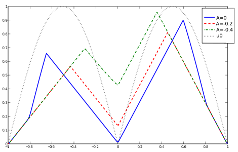
In Fig. 3, we show the numerical solution at time $t=0.1$ and $t=2$ for different choices of the parameter $A$ on the junction point $x=(0,0)$. We can observe as the asymmetry of the Hamiltonian with respect to the origin induces an asymmetric behavior of the solution. We can also observe how the choice of parameter $A$ influences globally the value function of the problem. In fact, when $A=0$ the optimal control in $x=0$ is simply $\alpha_{0}=0$ that corresponds to a zero cost, and since $u_{0}(0)=0$, the solution $u(t,0)=0$ for each $t\in[0,T].$ In the case of $A<0$ the situation is different: the control $\alpha_{0}=0$ does not correspond to a null cost. A trajectory, which remains on the junction point, entails a cost. Furthermore, we observe that for values of $|A|$ sufficiently large, the stationary solution does not change anymore. This is due to the fact that remaining in the junction point is no more a convenient choice.

In the case of $A=0$ and $A=-0.2$, we show the convergence rates. In absence of an analytic exact solution, we compare the approximated solution $w(T,x)$ with an approximation $u(T,x)$ obtained on a very fine grid with $\Delta x=10^{-4}$ and $\Delta t=\Delta x$. We evaluate the error with respect to the uniform discrete norm defined as following

$$E_{\infty}^{\Delta}:=\underset{x\in J^{\Delta x}}{\max}(|w(T,x)-u(T,x)|).$$ (64)

Figure 4: Graphic of $E_{\infty}^{\Delta}$($\circ$) with respect the space step, together with the line $K\Delta x$. Left $A=0$, with $K=4.5$, right $A=-0.2$, with $K=2$.

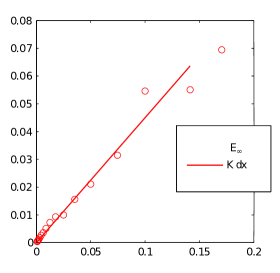
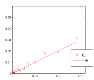
We show the results in Figure 4 for $T=0.2$ and $\Delta t=2.5\Delta x$. We observe in the case $A=0$ a linear decay of the $E^{\Delta}_{\infty}$ error, in particular, the $E^{\Delta}_{\infty}$ errors fit with a linear regression curve of ratio $K_{1}=4.5$. We also observe the same convergence order in the case $A=-0.2$, even though the linear convergence has a smaller ratio around $K_{1}=2$. We underline, by Theorem 4.1, that we aspect a convergence of order $1$ independently by the choice of ${\Delta t}$. This appears confirmed by the test.

Test 2

We consider still a simple junction network composed by three edges connecting the nodes $(0,1)$, $(-1,-1)$, $(1,-1)$ with the junction point placed in $(0,0)$.

Figure 5: Projection on the state coordinate plane of the Initial Condition (top left), numerical solution at time $t=0.4$ (top right), $t=0.8$ (bottom left) and $t=1.25$ (bottom right).

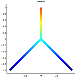
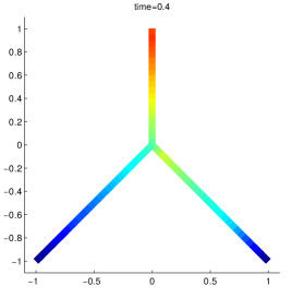
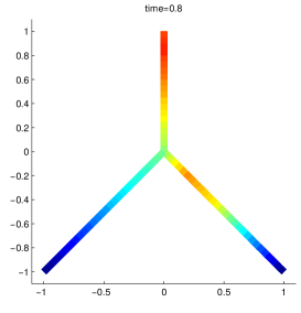
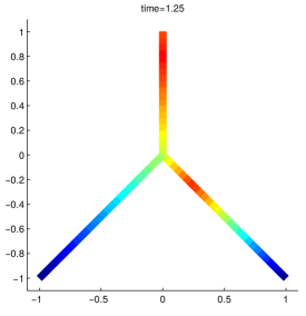
We denote by $J_{1}$ the edge connecting $(0,1)$ to $(0,0)$ and by $J_{2}$, $J_{3}$ the edges connecting $(0,0)$ to $(1,-1)$ and $(-1,-1)$, respectively. The cost function $L_{i},i=0,1,2,3$ are defined as follows

$$L_{i}(\alpha_{i})=\left\{\begin{array}[]{ll}\frac{\alpha_{i}^{2}}{2}+1&\hbox{ if }i=1,3,\\ \frac{\alpha_{i}^{2}}{2}+2&\hbox{ if }i=2,0.\end{array}\right.$$

We impose Dirichlet boundary conditions on the boundary nodes:

$$u(t,x)=\left\{\begin{array}[]{ll}0&\hbox{ if }x=\{(-1,-1),(1,-1)\}\\ \sqrt{2}+1&\hbox{ if }x=\{(0,1)\}.\end{array}\right.$$

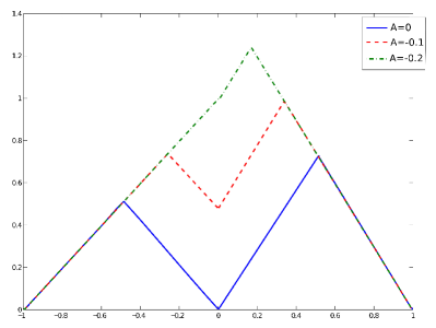
The initial value $u_{0}$ is chosen as the restriction of $1+x_{2}$ on $J$, where we denote $(x_{1},x_{2})=x$. In Figure 5, we show the color map of the initial condition and of the numerical solution at time $t=0.4,0.8,1.25$, projected on the state coordinate plane. We can observe that the initial datum $u_{0}$ (Fig. 5 left/top) quickly evolves to the stationary solution (Fig. 5 right/bottom), which represents a weighted distance from the boundary points, with exit costs equal to the Dirichlet boundary conditions.

We compare the approximate solution at $T=2$ with the exact solution of the corresponding stationary problem; this makes sense since the approximate solution has already reached the steady state at time $T=2$. The exact steady state solution is

$$u(x)=\left\{\begin{array}[]{ll}\sqrt{2}+x_{2},&\hbox{ if }x\in J_{1},\\ \min\left(2\sqrt{(x_{1}-1)^{2}+(x_{2}+1)^{2}},\sqrt{2}+2\sqrt{x_{1}^{2}+x_{2}^{2}}\right),&\hbox{ if }x\in J_{2},\\ \sqrt{(x_{1}+1)^{2}+(x_{2}+1)^{2}},&\hbox{ if }x\in J_{3}.\end{array}\right.$$ (65)

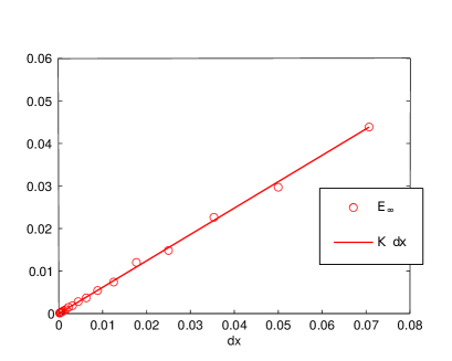
In Figure 6, we show the behavior of the error (64) for various values of $\Delta$, fixing the ratio between the spatial and the time step as $\Delta t=2.5\Delta x$. We underline that this is possible thanks to the stability property of SL methods for large time steps (i.e. the classical hyperbolic CFL condition falcone2014semi may not be verified). We observe as in the first test a linear decay of the $E^{\Delta}_{\infty}$ error.

Figure 6: Graphic of $E_{\infty}^{\Delta}$($\circ$) with respect the space step, together with the line $K\Delta x$ with $K=6.5$.

Test 3

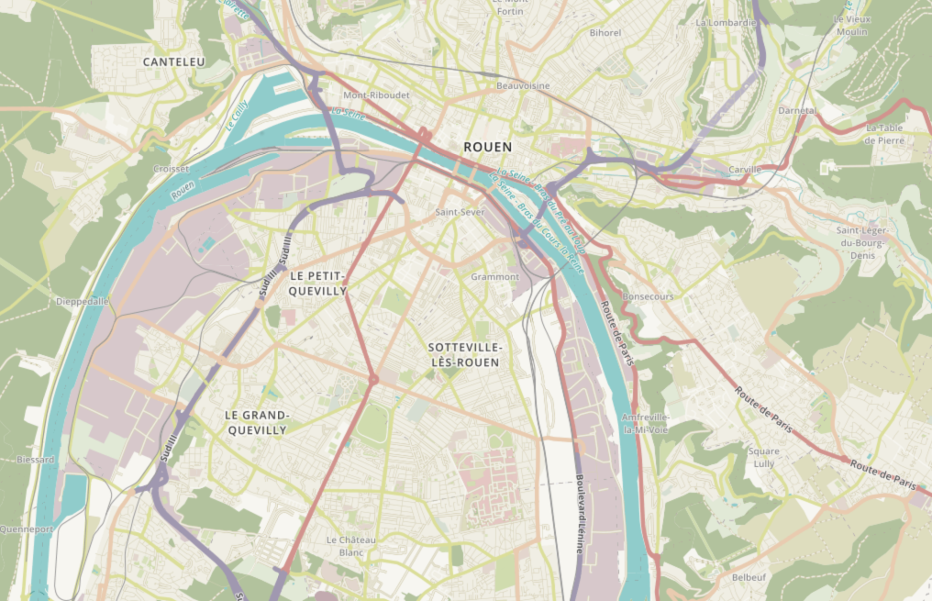
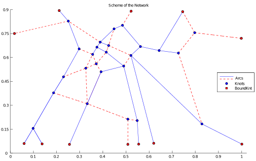
We conclude this section with a more realistic test where multiple edges are composing a complex traffic network. We consider the main network of the city of Rouen (Figure 7, above) and after some simplifications, we arrive at the network represented in Figure 7, below. Here the edges in continuous blue line are large capacity roads, and in dashed red are smaller roads. The network is contained in the planar set $[0,1200]\times[0,2100]\subset{\mathbb{R}}^{2}$, that corresponds to the pixels of the reference map from which we extracted the network. For practical purposes, we scale it in the domain $[0,1]^{2}$.

Figure 7: Map of the city of Rouen and simplified network modeling the structure of the road networks. In blue/solid line the bigger roads, in red/dotted line the smaller roads. The map $\copyright$ OpenStreetMap contributors.

Using the traffic flow interpretation of an HJ equation, as sketched in Section 5, we choose the initial datum $u(x,0)=v(x)$ where $v(x)$ is the solution of the following stationary HJ equation

$$\left\{\begin{array}[]{ll}|v_{x}(x)|=0.7-\frac{(x-(0.5,0.5))^{2}}{2},&x\in J\\ v(x)=0,&x\in\mathcal{B}.\end{array}\right.$$

This case can be viewed as a special case of the stationary state of (2), where the analysis is simpler since the Hamiltonian is continuous (cf. camilli2013approximation for a detailed presentation). This choice of the initial datum models higher concentration of vehicles in correspondence of the city center (center of the domain).

We are interested in the evolution of the density of the vehicles $\rho$. We could derive it using $\eqref{cum}$. This procedure may be nontrivial (cf. costeseque2015convergent ; imbert2013hamilton ) on the junctions and it is still a point that deserves further investigation. Instead, we adopt a numerical heuristic procedure using the relation $\rho(x,t)=-u_{x}(x,t)$ along every edge and defining

$$\rho(x,t)=-\sum_{i}\min(\partial_{i}u(x,t),0),\quad\hbox{if }x\in\mathcal{V}$$

where the spatial derivatives are approximated thorough standard finite differences. The numerical test that we present confirms that this procedure provides reasonable results.

We want to study the network in a case of an evacuation. We impose null Dirichlet boundary conditions on the exits of the network in correspondence of the red squares of Figure 7 (below). We adopt the simple Hamiltonian

$$H_{i}(p)=\left\{\begin{array}[]{ll}\frac{1}{\lambda_{i}}p^{2}-p&\hbox{ if $p\geq 0$ },\\ \frac{1}{\lambda_{i}}p^{2}+p&\hbox{ if $p<0$,}\end{array}\right.$$

where $\lambda_{i}$ is the capacity of the arc $i$ namely $\lambda_{i}=4/5$ in the red edges and $\lambda_{i}=1$ elsewhere.

Figure 8: Evolution of the approximation of the density of vehicles at time $t=0,0.5,1,1.5$.

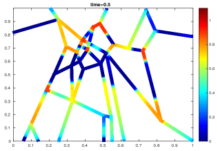
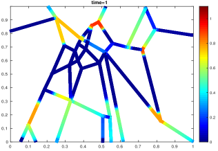
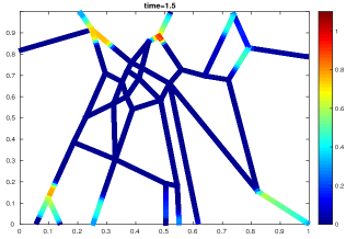
We observe that it is possible to obtain these Hamiltonians following imbert2013hamilton for the classic LWR model (cf. garavello2016models ) with flux $(1-\rho)\rho$ on the blue arcs and $(1-5/4\rho)\rho$ for the choice of $A=-0.4$. The red edges have then a reduced capacity compared to the blue ones.

We uniformly approximate the arcs using the discretization step ${\Delta x}=0.01$ and we sample the time with ${\Delta t}=0.05$. Due to the stability properties of the SL scheme no CFL condition is needed, and we can adopt large time steps, fundamental to approximate the behavior of the system for long time scenarios.

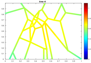
In Figure 8, we can see the initial distribution of the density and its evolution in various moments. We observe the following. First of all the density, starting from a smooth configuration (the initial data is for construction $\rho(t,x)=0.7-0.5(x-(0.5,0.5))^{2}$) rapidly concentrates reaching some areas of maximal density. Those congested areas typically appear before a junction point. It is an intrinsic characteristic already observed in traffic flows literature. This phenomenon can only become more evident in the case of merging bifurcations where the outgoing roads have a reduced capacity. This is the case of the junction in the proximity of the point $(0.5,0.82)$ where some congested areas are formed and take more time to disappear.

7 Acknowledgments

The first author was supported by the Indam GNCS project “Metodi numerici per equazioni iperboliche e cinetiche e applicazioni” and PGMO project VarPDEMFG. The second and third authors were partially supported by the European Union with the European regional development fund (ERDF, HN0002137) and by the Normandie Regional Council (via the M2NUM project).

References

- (1) Yves Achdou, Fabio Camilli, Alessandra Cutrì, and Nicoletta Tchou, Hamilton–jacobi equations constrained on networks, Nonlinear Differential Equations and Applications NoDEA 20 (2013), no. 3, 413–445.
- (2) Boris Andreianov, Kenneth Hvistendahl Karlsen, and Nils Henrik Risebro, A theory of l1-dissipative solvers for scalar conservation laws with discontinuous flux, Archive for rational mechanics and analysis 201 (2011), no. 1, 27–86.
- (3) Martino Bardi and Italo Capuzzo Dolcetta, Optimal control and viscosity solutions of Hamilton-Jacobi-Bellman equations, Birkauser, 1996.
- (4) Guy Barles, Ariela Briani, and Emmanuel Chasseigne, A bellman approach for two-domains optimal control problems in , ESAIM: Control, Optimisation and Calculus of Variations 19 (2013), no. 3, 710–739.
- (5) Guy Barles, Ariela Briani, Emmanuel Chasseigne, and Cyril Imbert, Flux-limited and classical viscosity solutions for regional control problems, arXiv preprint arXiv:1611.01977 (2016).
- (6) Guy Barles and Panagiotis E. Souganidis, Convergence of approximation schemes for fully nonlinear second order equations, Asymptotic Anal. 4 (1991), no. 3, 271–283.
- (7) Fabio Camilli, Elisabetta Carlini, and Claudio Marchi, A flame propagation model on a network with application to a blocking problem, to appear on DCDS-S October 2018 issue 11 (2018), no. 5.
- (8) Fabio Camilli, Adriano Festa, and Dirk Schieborn, An approximation scheme for a hamilton–jacobi equation defined on a network, Applied Numerical Mathematics 73 (2013), 33–47.
- (9) Fabio Camilli, Adriano Festa, and Silvia Tozza, A discrete hughes’ model for pedestrian flow on graphs, Networks & Heterogeneous Media 12 (2017), no. 1, 93–112.
- (10) Guillaume Costeseque, Jean-Patrick Lebacque, and Régis Monneau, A convergent scheme for hamilton–jacobi equations on a junction: application to traffic, Numerische Mathematik 129 (2015), no. 3, 405–447.
- (11) Emiliano Cristiani, Benedetto Piccoli, and Andrea Tosin, Multiscale modeling of granular flows with application to crowd dynamics, Multiscale Modeling & Simulation 9 (2011), no. 1, 155–182.
- (12) Maurizio Falcone and Roberto Ferretti, Semi-lagrangian approximation schemes for linear and hamilton-jacobi equations, vol. 133, SIAM, 2014.
- (13) Nicolas Forcadel and Wilfredo Salazar, Homogenization of second order discrete model and application to traffic flow, Differential and Integral Equations 28 (2015), no. 11/12, 1039–1068.
- (14) Mauro Garavello, Ke Han, and Benedetto Piccoli, Models for vehicular traffic on networks, vol. 9, American Institute of Mathematical Sciences (AIMS), Springfield, MO, 2016.
- (15) Mauro Garavello, Roberto Natalini, Benedetto Piccoli, and Andrea Terracina, Conservation laws with discontinuous flux, Networks & Heterogeneous Media 2 (2007), no. 1, 159–179.
- (16) Mauro Garavello and Benedetto Piccoli, Traffic flow on networks, vol. 1, American institute of mathematical sciences Springfield, 2006.
- (17) Jessica Guerand and Marwa Koumaiha, Error estimates for finite difference schemes associated with hamilton-jacobi equations on a junction, arXiv preprint arXiv:1502.07158 (2017).
- (18) Cyril Imbert and Régis Monneau, Flux-limited solutions for quasi-convex hamilton-jacobi equations on networks, Annales Scientifiques de l’ÉNS (2017), no. 50, 357–448.
- (19) Cyril Imbert, Régis Monneau, and Hasnaa Zidani, A hamilton-jacobi approach to junction problems and application to traffic flows, ESAIM: Control, Optimisation and Calculus of Variations 19 (2013), no. 1, 129–166.
- (20) Pierre-Louis Lions and Panagiotis Souganidis, Well-posedness for multi-dimensional junction problems with Kirchoff-type conditions, Atti Accad. Naz. Lincei Rend. Lincei Mat. Appl. 28 (2017), no. 4, 807–816. MR 3729588
- (21) Gordon F. Newell, A simplified theory of kinematic waves in highway traffic, part i: General theory, Transportation Research Part B: Methodological 27 (1993), no. 4, 281–287.
- (22) Alfio Quarteroni, Riccardo Sacco, and Fausto Saleri, Numerical mathematics, Texts in Applied Mathematics 37, Springer-Verlag Berlin Heidelberg, 2007.
- (23) Dirk Schieborn and Fabio Camilli, Viscosity solutions of eikonal equations on topological networks, Calculus of Variations and Partial Differential Equations (2013), 1–16.
- (24) Martin Treiber and Arne Kesting, Traffic flow dynamics, Traffic Flow Dynamics: Data, Models and Simulation, Springer-Verlag Berlin Heidelberg (2013).