Convolutional Generative Adversarial Networks with Binary Neurons for Polyphonic Music Generation
Abstract
It has been shown recently that deep convolutional generative adversarial networks (GANs) can learn to generate music in the form of piano-rolls, which represent music by binary-valued time-pitch matrices. However, existing models can only generate real-valued piano-rolls and require further post-processing, such as hard thresholding (HT) or Bernoulli sampling (BS), to obtain the final binary-valued results. In this paper, we study whether we can have a convolutional GAN model that directly creates binary-valued piano-rolls by using binary neurons. Specifically, we propose to append to the generator an additional refiner network, which uses binary neurons at the output layer. The whole network is trained in two stages. Firstly, the generator and the discriminator are pretrained. Then, the refiner network is trained along with the discriminator to learn to binarize the real-valued piano-rolls the pretrained generator creates. Experimental results show that using binary neurons instead of HT or BS indeed leads to better results in a number of objective measures. Moreover, deterministic binary neurons perform better than stochastic ones in both objective measures and a subjective test. The source code, training data and audio examples of the generated results can be found at https://salu133445.github.io/bmusegan/.
1 Introduction
Recent years have seen increasing research on symbolic-domain music generation and composition using deep neural networks [7]. Notable progress has been made to generate monophonic melodies [25, 27], lead sheets (i.e., melody and chords) [11, 8, 26], or four-part chorales [14]. To add something new to the table and to increase the polyphony and the number of instruments of the generated music, we attempt to generate piano-rolls in this paper, a music representation that is more general (e.g., comparing to leadsheets) yet less studied in recent work on music generation. As Figure 1 shows, we can consider an -track piano-roll as a collection of binary time-pitch matrices indicating the presence of pitches per time step for each track.
Dr.
Pi.
Gu.
Ba.
En.
Re.
S.L.
S.P.
Dr.
Pi.
Gu.
Ba.
En.
Re.
S.L.
S.P.
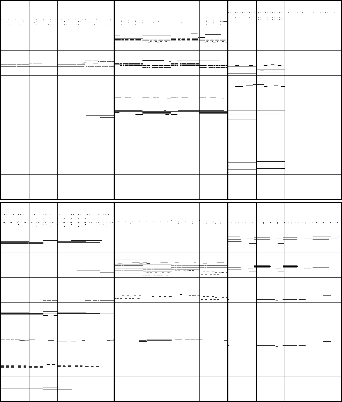
Generating piano-rolls is challenging because of the large number of possible active notes per time step and the involvement of multiple instruments. Unlike a melody or a chord progression, which can be viewed as a sequence of note/chord events and be modeled by a recurrent neural network (RNN) [21, 24], the musical texture in a piano-roll is much more complicated (see Figure 1). While RNNs are good at learning the temporal dependency of music, convolutional neural networks (CNNs) are usually considered better at learning local patterns [18].
For this reason, in our previous work [10], we used a convolutional generative adversarial network (GAN) [12] to learn to generate piano-rolls of five tracks. We showed that the model generates music that exhibit drum patterns and plausible note events. However, musically the generated result is still far from satisfying to human ears, scoring around on average on a five-level Likert scale in overall quality in a user study [10].111Another related work on generating piano-rolls, as presented by Boulanger-Lewandowski et al. [6], replaced the output layer of an RNN with conditional restricted Boltzmann machines (RBMs) to model high-dimensional sequences and applied the model to generate piano-rolls sequentially (i.e. one time step after another).
There are several ways to improve upon this prior work. The major topic we are interested in is the introduction of the binary neurons (BNs) [1, 4] to the model. We note that conventional CNN designs, also the one adopted in our previous work [10], can only generate real-valued predictions and require further postprocessing at test time to obtain the final binary-valued piano-rolls.222Such binarization is typically not needed for an RNN or an RBM in polyphonic music generation, since an RNN is usually used to predict pre-defined note events [22] and an RBM is often used with binary visible and hidden units and sampled by Gibbs sampling [6, 20]. This can be done by either applying a hard threshold (HT) on the real-valued predictions to binarize them (which was done in [10]), or by treating the real-valued predictions as probabilities and performing Bernoulli sampling (BS).
However, we note that such naïve methods for binarizing a piano-roll can easily lead to overly-fragmented notes. For HT, this happens when the original real-valued piano-roll has many entries with values close to the threshold. For BS, even an entry with low probability can take the value 1, due to the stochastic nature of probabilistic sampling.
The use of BNs can mitigate the aforementioned issue, since the binarization is part of the training process. Moreover, it has two potential benefits:
-
•
In [10], binarization of the output of the generator in GAN is done only at test time not at training time (see Section 2.1 for a brief introduction of GAN). This makes it easy for the discriminator in GAN to distinguish between the generated piano-rolls (which are real-valued in this case) and the real piano-rolls (which are binary). With BNs, the binarization is done at training time as well, so can focus on extracting musically relevant features.
-
•
Due to BNs, the input to the discriminator in GAN at training time is binary instead of real-valued. This effectively reduces the model space from to , where is the product of the number of time steps and the number of possible pitches. Training may be easier as the model space is substantially smaller, as Figure 2 illustrates.
Specifically, we propose to append to the end of a refiner network that uses either deterministic BNs (DBNs) or stocahstic BNs (SBNs) at the output layer. In this way, makes real-valued predictions and binarizes them. We train the whole network in two stages: in the first stage we pretrain and and then fix ; in the second stage, we train and fine-tune . We use residual blocks [16] in to make this two-stage training feasible (see Section 3.3).
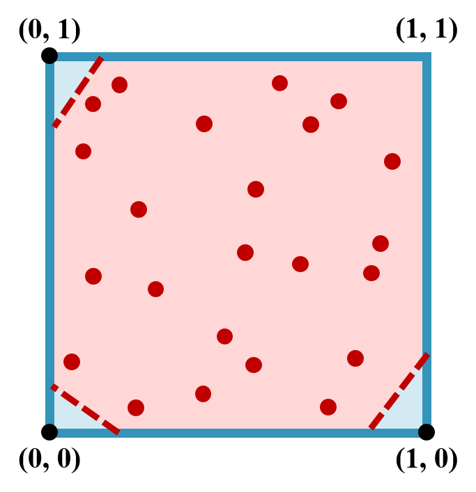
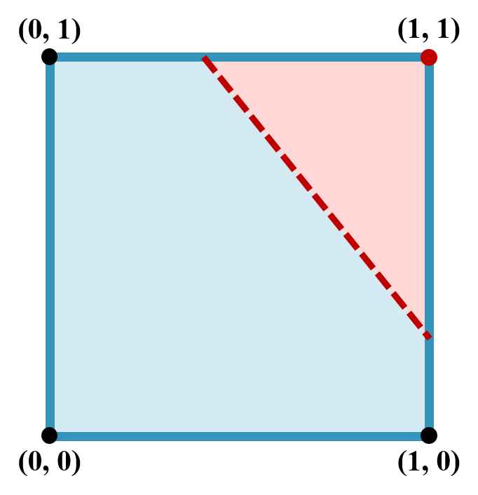
As minor contributions, we use a new shared/private design of and that cannot be found in [10]. Moreover, we add to two streams of layers that provide onset/offset and chroma information (see Sections 3.2 and 3.4).
The proposed model is able to directly generate binary-valued piano-rolls at test time. Our analysis shows that the generated results of our model with DBNs features fewer overly-fragmented notes as compared with the result of using HT or BS. Experimental results also show the effectiveness of the proposed two-stage training strategy compared to either a joint or an end-to-end training strategy.
2 Background
2.1 Generative Adversarial Networks
A generative adversarial network (GAN) [12] has two core components: a generator and a discriminator . The former takes as input a random vector sampled from a prior distribution and generates a fake sample . takes as input either real data or fake data generated by . During training time, learns to distinguish the fake samples from the real ones, whereas learns to fool .
An alternative form called WGAN was later proposed with the intuition to estimate the Wasserstein distance between the real and the model distributions by a deep neural network and use it as a critic for the generator [2]. The objective function for WGAN can be formulated as:
| (1) |
where denotes the real data distribution. In order to enforce Lipschitz constraints on the discriminator, which is required in the training of WGAN, Gulrajani et al. [13] proposed to add to the objective function of a gradient penalty (GP) term: , where is defined as sampling uniformly along straight lines between pairs of points sampled from and the model distribution . Empirically they found it stabilizes the training and alleviates the mode collapse issue, compared to the weight clipping strategy used in the original WGAN. Hence, we employ WGAN-GP [13] as our generative framework.
2.2 Stochastic and Deterministic Binary Neurons
Binary neurons (BNs) are neurons that output binary-valued predictions. In this work, we consider two types of BNs: deterministic binary neurons (DBNs) and stochastic binary neurons (SBNs). DBNs act like neurons with hard thresholding functions as their activation functions. We define the output of a DBN for a real-valued input as:
| (2) |
where denotes the unit step function and is the logistic sigmoid function. SBNs, in contrast, binarize an input according to a probability, defined as:
| (3) |
where denotes a uniform distribution.

2.3 Straight-through Estimator
Computing the exact gradients for either DBNs or SBNs, however, is intractable. For SBNs, it requires the computation of the average loss over all possible binary samplings of all the SBNs, which is exponential in the total number of SBNs. For DBNs, the threshold function in Eq. (2) is non-differentiable. Therefore, the flow of backpropagation used to train parameters of the network would be blocked.
A few solutions have been proposed to address this issue [1, 4]. One strategy is to replace the non-differentiable functions, which are used in the forward pass, by differentiable functions (usually called the estimators) in the backward pass. An example is the straight-through (ST) estimator proposed by Hinton [17]. In the backward pass, ST simply treats BNs as identify functions and ignores their gradients. A variant of the ST estimator is the sigmoid-adjusted ST estimator [9], which multiplies the gradients in the backward pass by the derivative of the sigmoid function. Such estimators were originally proposed as regularizers [17] and later found promising for conditional computation [4]. We use the sigmoid-adjusted ST estimator in training neural networks with BNs and found it empirically works well for our generation task as well.
3 Proposed Model
3.1 Data Representation
Following [10], we use the multi-track piano-roll representation. A multi-track piano-roll is defined as a set of piano-rolls for different tracks (or instruments). Each piano-roll is a binary-valued score-like matrix, where its vertical and horizontal axes represent note pitch and time, respectively. The values indicate the presence of notes over different time steps. For the temporal axis, we discard the tempo information and therefore every beat has the same length regardless of tempo.
3.2 Generator
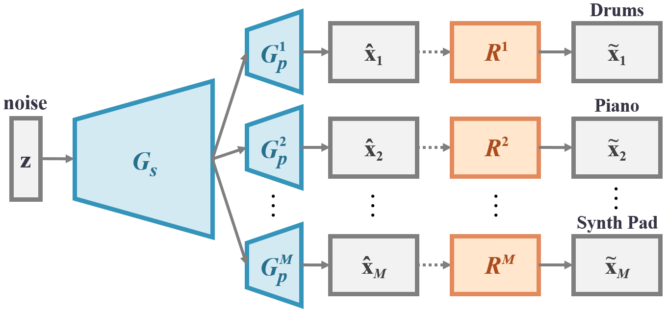
As Figure 3 shows, the generator consists of a “s”hared network followed by “p”rivate network , , one for each track. The shared generator first produces a high-level representation of the output musical segments that is shared by all the tracks. Each private generator then turns such abstraction into the final piano-roll output for the corresponding track. The intuition is that different tracks have their own musical properties (e.g., textures, common-used patterns), while jointly they follow a common, high-level musical idea. The design is different from [10] in that the latter does not include a shared in early layers.

| Dr. [10pt]Pi. [10pt]Gu. [10pt]Ba. [10pt]En. [4pt] | 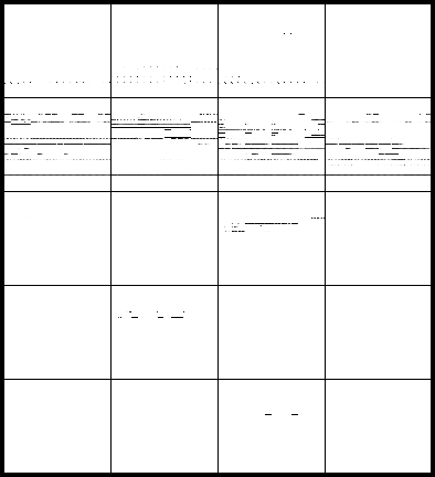 |
 |
 |
 |
 |
|---|---|---|---|---|---|
| (a) raw predictions | (b) pretrained (+BS) | (c) pretrained (+HT) | (d) proposed (+SBNs) | (d) proposed (+DBNs) |
3.3 Refiner
The refiner is composed of private networks , , again one for each track. The refiner aims to refine the real-valued outputs of the generator, , into binary ones, , rather than learning a new mapping from to the data space. Hence, we draw inspiration from residual learning and propose to construct the refiner with a number of residual units [16], as shown in Figure 4. The output layer (i.e. the final layer) of the refiner is made up of either DBNs or SBNs.
3.4 Discriminator
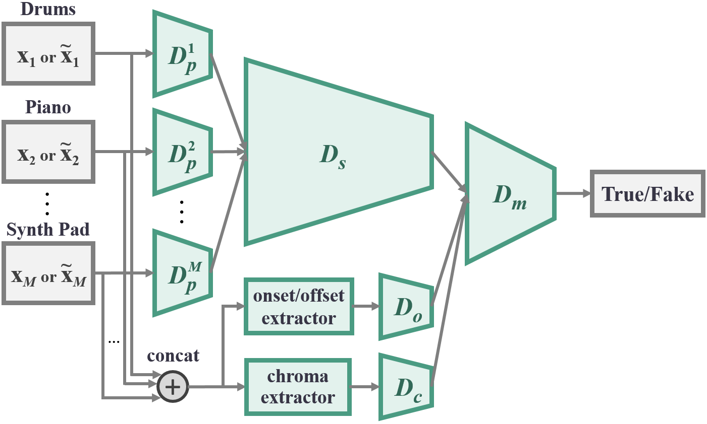
Similar to the generator, the discriminator consists of private network , , one for each track, followed by a shared network , as shown in Figure 5. Each private network first extracts low-level features from the corresponding track of the input piano-roll. Their outputs are concatenated and sent to the shared network to extract higher-level abstraction shared by all the tracks. The design differs from [10] in that only one (shared) discriminator was used in [10] to evaluate all the tracks collectively. We intend to evaluate such a new shared/private design in Section 4.5.
As a minor contribution, to help the discriminator extract musically-relevant features, we propose to add to the discriminator two more streams, shown in the lower half of Figure 5. In the first onset/offset stream, the differences between adjacent elements in the piano-roll along the time axis are first computed, and then the resulting matrix is summed along the pitch axis, which is finally fed to .
In the second chroma stream, the piano-roll is viewed as a sequence of one-beat-long frames. A chroma vector is then computed for each frame and jointly form a matrix, which is then be fed to . Note that all the operations involved in computing the chroma and onset/offset features are differentiable, and thereby we can still train the whole network by backpropagation.
Finally, the features extracted from the three streams are concatenated and fed to to make the final prediction.
3.5 Training
We propose to train the model in a two-stage manner: and are pretrained in the first stage; is then trained along with (fixing ) in the second stage. Other training strategies are discussed and compared in Section 4.4.
4 Analysis of the Generated Results
4.1 Training Data & Implementation Details
The Lakh Pianoroll Dataset (LPD) [10]333https://salu133445.github.io/lakh-pianoroll-dataset/ contains 174,154 multi-track piano-rolls derived from the MIDI files in the Lakh MIDI Dataset (LMD) [23].444http://colinraffel.com/projects/lmd/ In this paper, we use a cleansed subset (LPD-cleansed) as the training data, which contains 21,425 multi-track piano-rolls that are in 4/4 time and have been matched to distinct entries in Million Song Dataset (MSD) [5]. To make the training data cleaner, we consider only songs with an alternative tag. We randomly pick six four-bar phrases from each song, which leads to the final training set of 13,746 phrases from 2,291 songs.
We set the temporal resolution to 24 time steps per beat to cover common temporal patterns such as triplets and 32th notes. An additional one-time-step-long pause is added between two consecutive (i.e. without a pause) notes of the same pitch to distinguish them from one single note. The note pitch has 84 possibilities, from C1 to B7.
We categorize all instruments into drums and sixteen instrument families according to the specification of General MIDI Level 1.555https://www.midi.org/specifications/item/gm-level-1-sound-set We discard the less popular instrument families in LPD and use the following eight tracks: Drums, Piano, Guitar, Bass, Ensemble, Reed, Synth Lead and Synth Pad. Hence, the size of the target output tensor is (bar) (time step) (pitch) (track).
| training data | pretrained | proposed | joint | end-to-end | ablated-I | ablated-II | |||||||
|---|---|---|---|---|---|---|---|---|---|---|---|---|---|
| BS | HT | SBNs | DBNs | SBNs | DBNs | SBNs | DBNs | BS | HT | BS | HT | ||
| QN | 0.88 | 0.67 | 0.72 | 0.42 | 0.78 | 0.18 | 0.55 | 0.67 | 0.28 | 0.61 | 0.64 | 0.35 | 0.37 |
| PP | 0.48 | 0.20 | 0.22 | 0.26 | 0.45 | 0.19 | 0.19 | 0.16 | 0.29 | 0.19 | 0.20 | 0.14 | 0.14 |
| TD | 0.96 | 0.98 | 1.00 | 0.99 | 0.87 | 0.95 | 1.00 | 1.40 | 1.10 | 1.00 | 1.00 | 1.30 | 1.40 |
(Underlined and bold font indicate respectively the top and top-three entries with values closest to those shown in the ‘training data’ column.)
Both and are implemented as deep CNNs (see Appendix A for the detailed network architectures). The length of the input random vector is . consists of two residual units [16] shown in Figure 6. Following [13], we use the Adam optimizer [19] and only apply batch normalization to and . We apply the slope annealing trick [9] to networks with BNs, where the slope of the sigmoid function in the sigmoid-adjusted ST estimator is multiplied by after each epoch. The batch size is except for the first stage in the two-stage training setting, where the batch size is .
| (a) |  |
|---|---|
| (b) |  |
| (c) |  |
| (d) |  |
| (e) |  |
4.2 Objective Evaluation Metrics
We generate 800 samples for each model (see Appendix C for sample generated results) and use the following metrics proposed in [10] for evaluation. We consider a model better if the average metric values of the generated samples are closer to those computed from the training data.
-
•
Qualified note rate (QN) computes the ratio of the number of the qualified notes (notes no shorter than three time steps, i.e., a 32th note) to the total number of notes. Low QN implies overly-fragmented music.
-
•
Polyphonicity (PP) is defined as the ratio of the number of time steps where more than two pitches are played to the total number of time steps.
-
•
Tonal distance (TD) measures the distance between the chroma features (one for each beat) of a pair of tracks in the tonal space proposed in [15]. In what follows, we only report the TD between the piano and the guitar, for they are the two most used tracks.
4.3 Comparison of Binarization Strategies
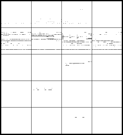
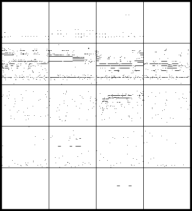
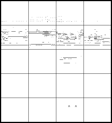
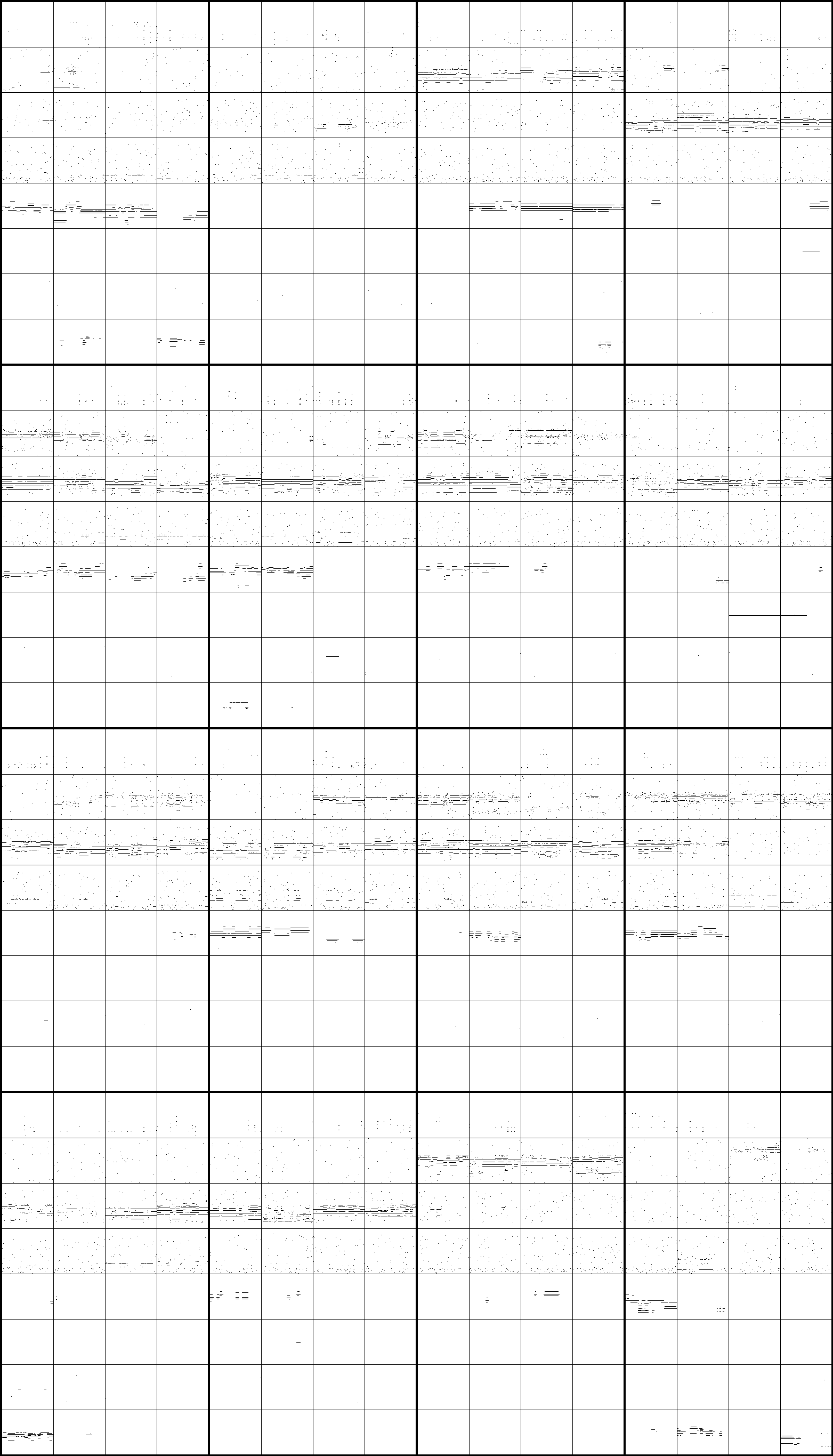
We compare the proposed model with two common test-time binarization strategies: Bernoulli sampling (BS) and hard thresholding (HT). Some qualitative results are provided in Figures 7 and 8. Moreover, we present in Table 1 a quantitative comparison among them.
Both qualitative and quantitative results show that the two test-time binarization strategies can lead to overly-fragmented piano-rolls (see the “pretrained” ones). The proposed model with DBNs is able to generate piano-rolls with a relatively small number of overly-fragmented notes (a QN of ; see Table 1) and to better capture the statistical properties of the training data in terms of PP. However, the proposed model with SBNs produces a number of random-noise-like artifacts in the generated piano-rolls, as can be seen in Figure 8(d), leading to a low QN of . We attribute to the stochastic nature of SBNs. Moreover, we can also see from Figure 9 that only the proposed model with DBNs keeps improving after the second-stage training starts in terms of QN and PP.
(a) 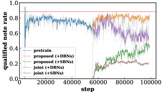
(b) 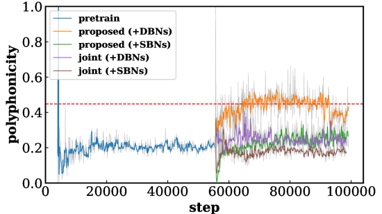
4.4 Comparison of Training Strategies
We consider two alternative training strategies:
-
•
joint: pretrain and in the first stage, and then train and (like viewing as part of ) jointly with in the second stage.
-
•
end-to-end: train , and jointly in one stage.
As shown in Table 1, the models with DBNs trained using the joint and end-to-end training strategies receive lower scores as compared to the two-stage training strategy in terms of QN and PP. We can also see from Figure 9(a) that the model with DBNs trained using the joint training strategy starts to degenerate in terms of QN at about 10,000 steps after the second-stage training begins.
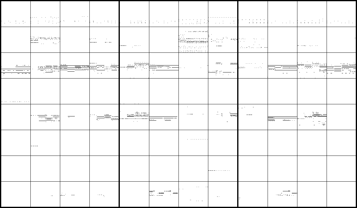
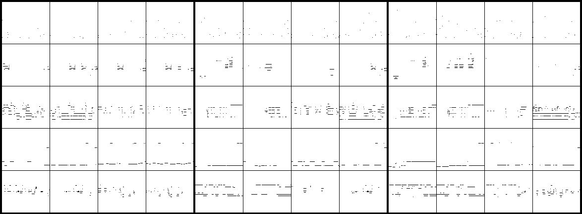
Figure 10 shows some qualitative results for the end-to-end models. It seems that the models learn the proper pitch ranges for different tracks. We also see some chord-like patterns in the generated piano-rolls. From Table 1 and Figure 10, in the end-to-end training setting SBNs are not inferior to DBNs, unlike the case in the two-stage training. Although the generated results appear preliminary, to our best knowledge this represents the first attempt to generate such high dimensional data with BNs from scratch (see remarks in Appendix D).
Dr.
Pi.
Gu.
Ba.
En.
Re.
S.L.
S.P.
Dr.
Pi.
Gu.
Ba.
En.
4.5 Effects of the Shared/private and Multi-stream Design of the Discriminator
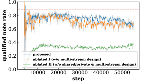
We compare the proposed model with two ablated versions: the ablated-I model, which removes the onset/offset and chroma streams, and the ablated-II model, which uses only a shared discriminator without the shared/private and multi-stream design (i.e., the one adopted in [10]).666The number of parameters for the proposed, ablated-I and ablated-II models is 3.7M, 3.4M and 4.6M, respectively. Note that the comparison is done by applying either BS or HT (not BNs) to the first-stage pretrained models.
As shown in Table 1, the proposed model (see “pretrained”) outperforms the two ablated versions in all three metrics. A lower QN for the proposed model as compared to the ablated-I model suggests that the onset/offset stream can alleviate the overly-fragmented note problem. Lower TD for the proposed and ablated-I models as compared to the ablated-II model indicates that the shared/private design better capture the intertrack harmonicity. Figure 11 also shows that the proposed and ablated-I models learn faster and better than the ablated-II model in terms of QN.
4.6 User Study
Finally, we conduct a user study involving 20 participants recruited from the Internet. In each trial, each subject is asked to compare two pieces of four-bar music generated from scratch by the proposed model using SBNs and DBNs, and vote for the better one in four measures. There are five trials in total per subject. We report in Table 2 the ratio of votes each model receives. The results show a preference to DBNs for the proposed model.
| with SBNs | with DBNs | |
|---|---|---|
| completeness* | 0.19 | 0.81 |
| harmonicity | 0.44 | 0.56 |
| rhythmicity | 0.56 | 0.44 |
| overall rating | 0.16 | 0.84 |
*We asked, “Are there many overly-fragmented notes?”
5 Discussion and Conclusion
We have presented a novel convolutional GAN-based model for generating binary-valued piano-rolls by using binary neurons at the output layer of the generator. We trained the model on an eight-track piano-roll dataset. Analysis showed that the generated results of our model with deterministic binary neurons features fewer overly-fragmented notes as compared with existing methods. Though the generated results appear preliminary and lack musicality, we showed the potential of adopting binary neurons in a music generation system.
In future work, we plan to further explore the end-to-end models and add recurrent layers to the temporal model. It might also be interesting to use BNs for music transcription [3], where the desired outputs are also binary-valued.
References
- [1] Binary stochastic neurons in tensorflow, 2016. Blog post on R2RT blog. [Online] https://r2rt.com/binary-stochastic-neurons-in-tensorflow.html.
- [2] Martin Arjovsky, Soumith Chintala, and Léon Bottou. Wasserstein generative adversarial networks. In Proc. ICML, 2017.
- [3] Emmanouil Benetos, Simon Dixon, Dimitrios Giannoulis, Holger Kirchhoff, and Anssi Klapuri. Automatic music transcription: challenges and future directions. Journal of Intelligent Information Systems, 41(3):407–434, 2013.
- [4] Yoshua Bengio, Nicholas Léonard, and Aaron C. Courville. Estimating or propagating gradients through stochastic neurons for conditional computation. arXiv preprint arXiv:1308.3432, 2013.
- [5] Thierry Bertin-Mahieux, Daniel P.W. Ellis, Brian Whitman, and Paul Lamere. The Million Song Dataset. In Proc. ISMIR, 2011.
- [6] Nicolas Boulanger-Lewandowski, Yoshua Bengio, and Pascal Vincent. Modeling temporal dependencies in high-dimensional sequences: Application to polyphonic music generation and transcription. In Proc. ICML, 2012.
- [7] Jean-Pierre Briot, Gaëtan Hadjeres, and François Pachet. Deep learning techniques for music generation: A survey. arXiv preprint arXiv:1709.01620, 2017.
- [8] Hang Chu, Raquel Urtasun, and Sanja Fidler. Song from PI: A musically plausible network for pop music generation. In Proc. ICLR, Workshop Track, 2017.
- [9] Junyoung Chung, Sungjin Ahn, and Yoshua Bengio. Hierarchical multiscale recurrent neural networks. In Proc. ICLR, 2017.
- [10] Hao-Wen Dong, Wen-Yi Hsiao, Li-Chia Yang, and Yi-Hsuan Yang. MuseGAN: Symbolic-domain music generation and accompaniment with multi-track sequential generative adversarial networks. In Proc. AAAI, 2018.
- [11] Douglas Eck and Jürgen Schmidhuber. Finding temporal structure in music: Blues improvisation with LSTM recurrent networks. In Proc. IEEE Workshop on Neural Networks for Signal Processing, 2002.
- [12] Ian J. Goodfellow et al. Generative adversarial nets. In Proc. NIPS, 2014.
- [13] Ishaan Gulrajani, Faruk Ahmed, Martin Arjovsky, Vincent Dumoulin, and Aaron Courville. Improved training of Wasserstein GANs. In Proc. NIPS, 2017.
- [14] Gaëtan Hadjeres, François Pachet, and Frank Nielsen. DeepBach: A steerable model for Bach chorales generation. In Proc. ICML, 2017.
- [15] Christopher Harte, Mark Sandler, and Martin Gasser. Detecting harmonic change in musical audio. In Proc. ACM MM Workshop on Audio and Music Computing Multimedia, 2006.
- [16] Kaiming He, Xiangyu Zhang, Shaoqing Ren, and Jian Sun. Identity mappings in deep residual networks. In Proc. ECCV, 2016.
- [17] Geoffrey Hinton. Neural networks for machine learning—using noise as a regularizer (lecture 9c), 2012. Coursera, video lectures. [Online] https://www.coursera.org/lecture/neural-networks/using-noise-as-a-regularizer-7-min-wbw7b.
- [18] Cheng-Zhi Anna Huang, Tim Cooijmans, Adam Roberts, Aaron Courville, and Douglas Eck. Counterpoint by convolution. In Proc. ISMIR, 2017.
- [19] Diederik P. Kingma and Jimmy Ba. Adam: A method for stochastic optimization. arXiv preprint arXiv:1412.6980, 2014.
- [20] Stefan Lattner, Maarten Grachten, and Gerhard Widmer. Imposing higher-level structure in polyphonic music generation using convolutional restricted Boltzmann machines and constraints. Journal of Creative Music Systems, 3(1), 2018.
- [21] Hyungui Lim, Seungyeon Rhyu, and Kyogu Lee. Chord generation from symbolic melody using BLSTM networks. In Proc. ISMIR, 2017.
- [22] Olof Mogren. C-RNN-GAN: Continuous recurrent neural networks with adversarial training. In NIPS Worshop on Constructive Machine Learning Workshop, 2016.
- [23] Colin Raffel. Learning-Based Methods for Comparing Sequences, with Applications to Audio-to-MIDI Alignment and Matching. PhD thesis, Columbia University, 2016.
- [24] Adam Roberts, Jesse Engel, Colin Raffel, Curtis Hawthorne, and Douglas Eck. A hierarchical latent vector model for learning long-term structure in music. In Proc. ICML, 2018.
- [25] Bob L. Sturm, João Felipe Santos, Oded Ben-Tal, and Iryna Korshunova. Music transcription modelling and composition using deep learning. In Proc. CSMS, 2016.
- [26] Li-Chia Yang, Szu-Yu Chou, and Yi-Hsuan Yang. MidiNet: A convolutional generative adversarial network for symbolic-domain music generation. In Proc. ISMIR, 2017.
- [27] Lantao Yu, Weinan Zhang, Jun Wang, and Yong Yu. SeqGAN: Sequence generative adversarial nets with policy gradient. In Proc. AAAI, 2017.
APPENDIX
Appendix A Network Architectures
We show in Table 3 the network architectures for the generator , the discriminator , the onset/offset feature extractor , the chroma feature extractor and the discriminator for the ablated-II model.
Appendix B Samples of the Training Data
Figure 12 shows some sample eight-track piano-rolls seen in the training data.
Appendix C Sample Generated Piano-rolls
Appendix D Remarks on the End-to-end Models
After several trials, we found that the claim in the main text that an end-to-end training strategy cannot work well is not true with the following modifications to the network. However, a thorough analysis of the end-to-end models are beyond the scope of this paper.
-
•
remove the refiner network ()
-
•
use binary neurons (either DBNs or SBNs) in the last layer of the generator ()
-
•
reduce the temporal resolution by half to time steps per beat
-
•
use five-track (Drums, Piano, Guitar, Bass and Ensemble) piano-rolls as the training data
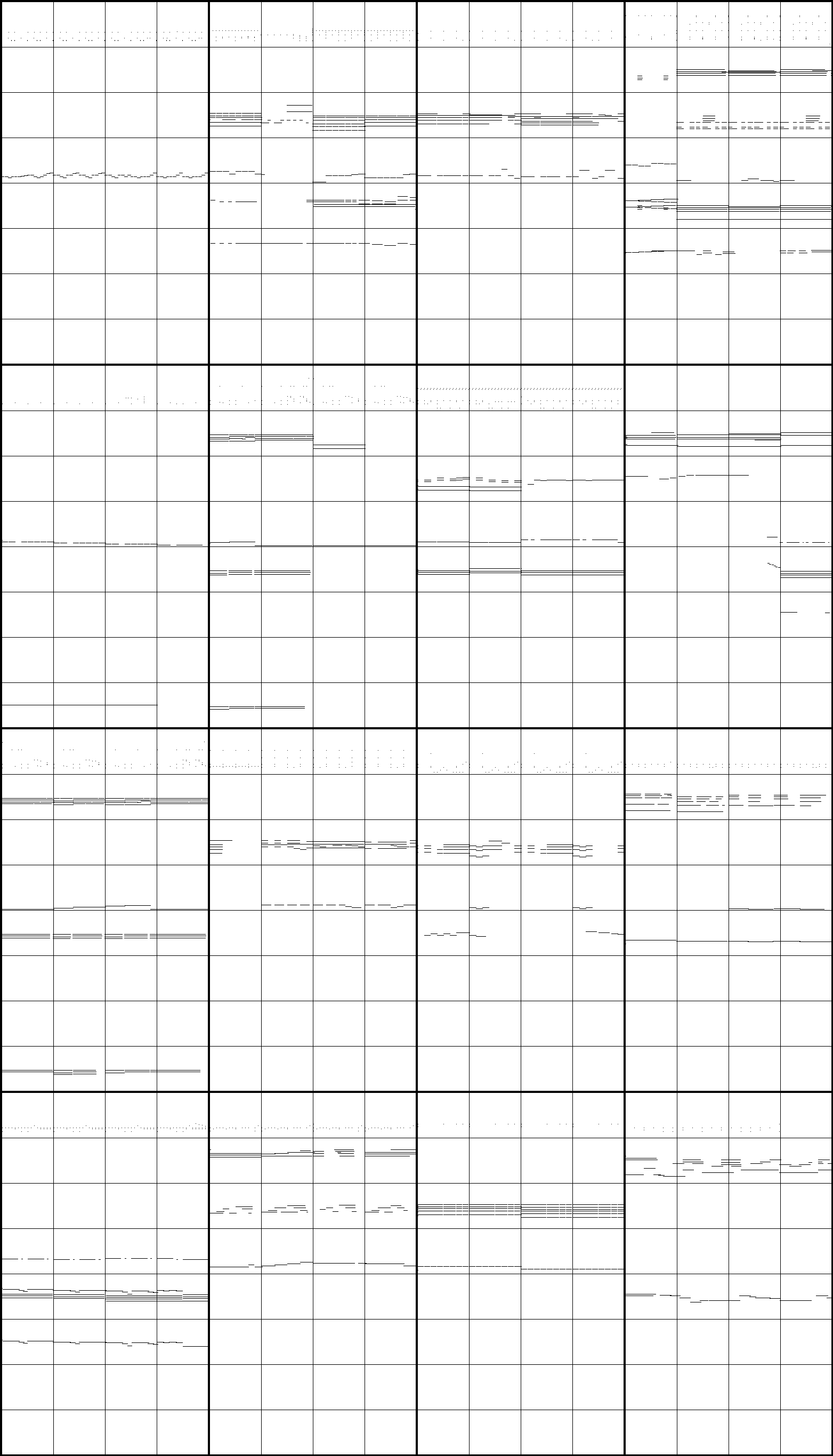
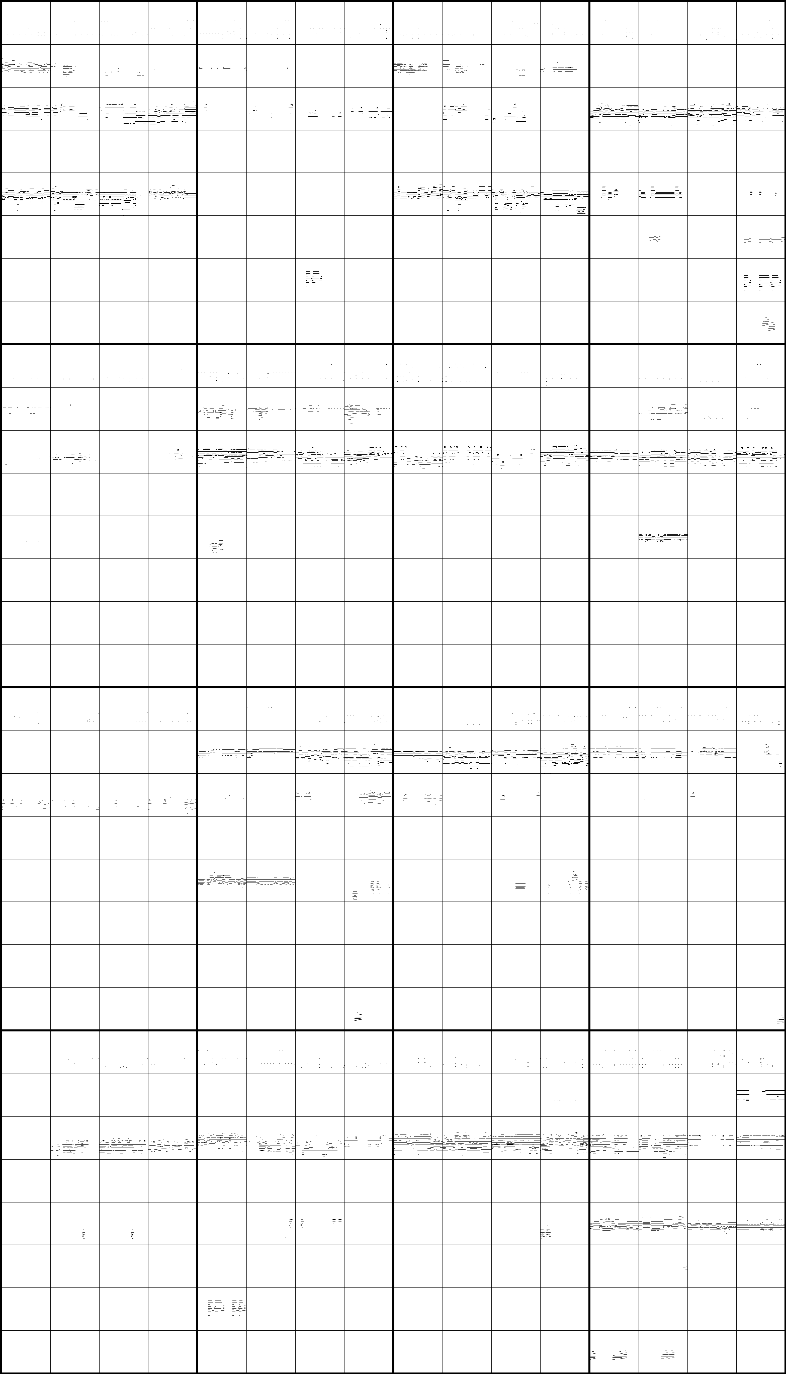
We show in Figure 15 some sample five-track piano-rolls generated by the modified end-to-end models with DBNs and SBNs.
| Input: | |||||||
|---|---|---|---|---|---|---|---|
| dense | |||||||
| reshape to channels | |||||||
| transconv | |||||||
| transconv | |||||||
| transconv | |||||||
| transconv | |||||||
| transconv | |||||||
| substream I | substream II | ||||||
| \cdashline2-7[1pt/1pt] transconv | |||||||
| transconv | |||||||
| concatenate along the channel axis | |||||||
| transconv | |||||||
| stack along the track axis | |||||||
| Output: | |||||||
(a) generator
| Input: | |||||||||
|---|---|---|---|---|---|---|---|---|---|
| split along the track axis | chroma stream | onset stream | |||||||
| substream I | substream II | ||||||||
| \cdashline2-7[1pt/1pt] conv | |||||||||
| conv | |||||||||
| concatenate along the channel axis | |||||||||
| conv | |||||||||
| concatenate along the channel axis | |||||||||
| conv | |||||||||
| conv | |||||||||
| concatenate along the channel axis | |||||||||
| conv | |||||||||
| dense | |||||||||
| dense | |||||||||
| Output: | |||||||||
(b) discriminator
| Input: | |||
|---|---|---|---|
| conv | |||
| conv | |||
| conv | |||
| Output: | |||
(c) onset/offset feature extractor
| Input: | |||
|---|---|---|---|
| conv | |||
| conv | |||
| Output: | |||
(d) chroma feature extractor
| Input: | |||
|---|---|---|---|
| conv | |||
| conv | |||
| conv | |||
| conv | |||
| conv | |||
| conv | |||
| conv | |||
| flatten to a vector | |||
| dense | |||
| Output: | |||
(e) discriminator for the ablated-II model
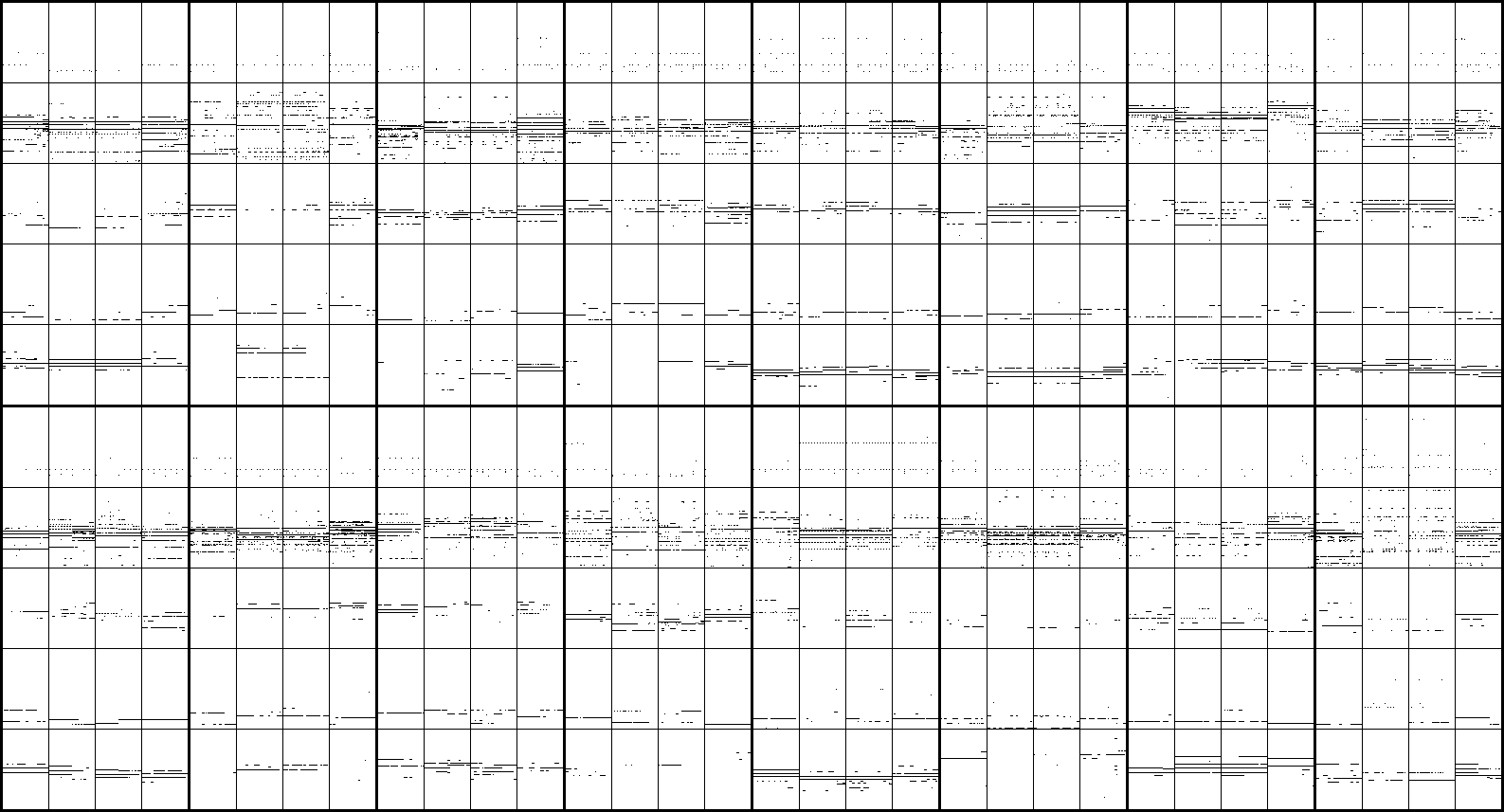
(a) modified end-to-end model (+DBNs)
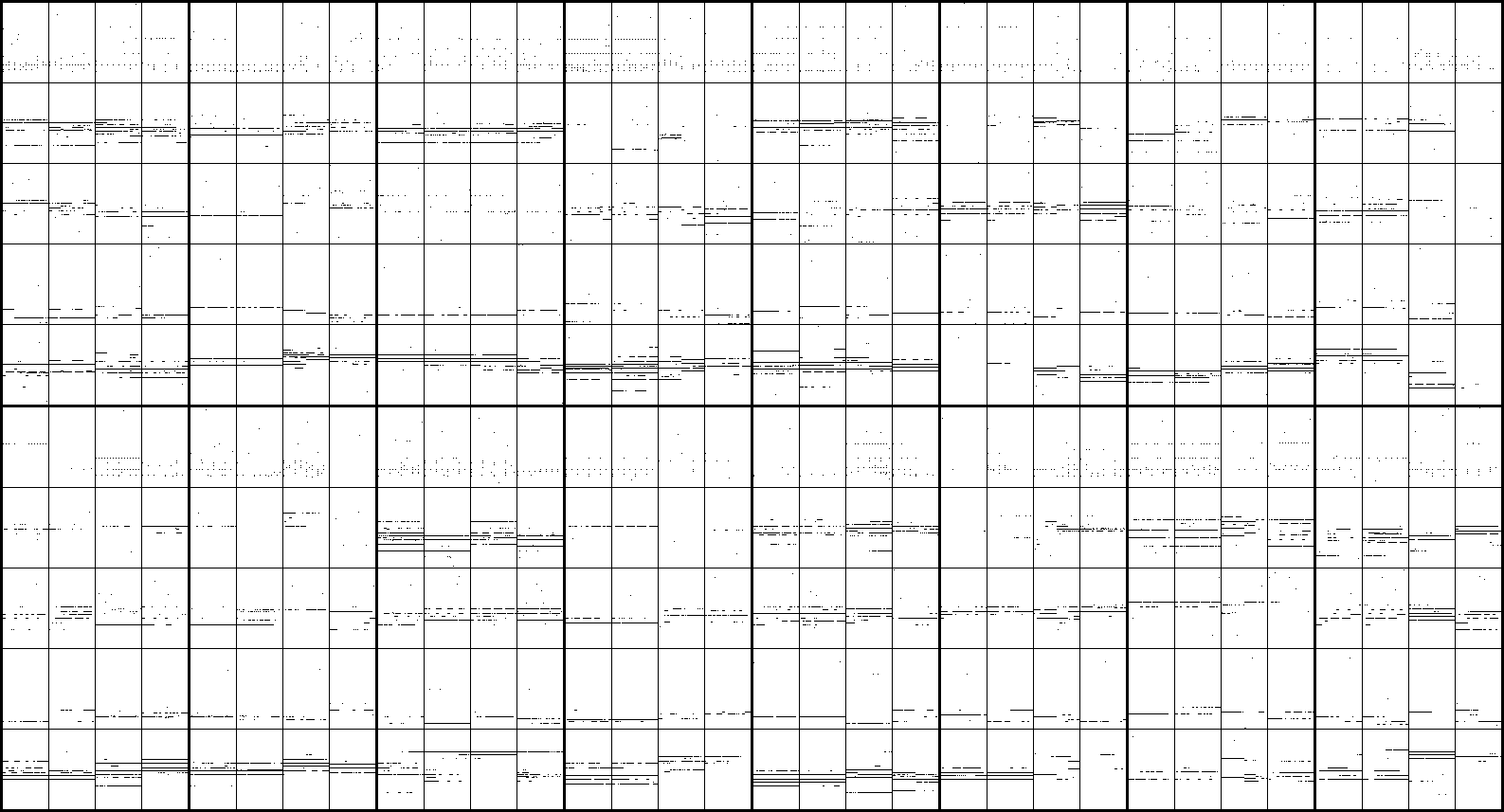
(b) modified end-to-end model (+SBNs)