Gaia Data Release 2: Using Gaia parallaxes
Abstract
Context. The second Gaia data release (Gaia DR2 ) provides precise five-parameter astrometric data (positions, proper motions, and parallaxes) for an unprecedented number of sources (more than billion, mostly stars). This new wealth of data will enable the undertaking of statistical analysis of many astrophysical problems that were previously infeasible for lack of reliable astrometry, and in particular because of the lack of parallaxes. However, the use of this wealth of astrometric data comes with a specific challenge: how can the astrophysical parameters of interest be properly inferred from these data?
Aims. The main focus of this paper, but not the only focus, is the issue of the estimation of distances from parallaxes, possibly combined with other information. We start with a critical review of the methods traditionally used to obtain distances from parallaxes and their shortcomings. Then we provide guidelines on how to use parallaxes more efficiently to estimate distances by using Bayesian methods. In particular we also show that negative parallaxes, or parallaxes with relatively large uncertainties still contain valuable information. Finally, we provide examples that show more generally how to use astrometric data for parameter estimation, including the combination of proper motions and parallaxes and the handling of covariances in the uncertainties.
Methods. The paper contains examples based on simulated Gaia data to illustrate the problems and the solutions proposed. Furthermore, the developments and methods proposed in the paper are linked to a set of tutorials included in the Gaia archive documentation that provide practical examples and a good starting point for the application of the recommendations to actual problems. In all cases the source code for the analysis methods is provided.
Results. Our main recommendation is to always treat the derivation of (astro-)physical parameters from astrometric data, in particular when parallaxes are involved, as an inference problem which should preferably be handled with a full Bayesian approach.
Conclusions. Gaia will provide fundamental data for many fields of astronomy. Further data releases will provide more data, and more precise data. Nevertheless, to fully use the potential it will always be necessary to pay careful attention to the statistical treatment of parallaxes and proper motions. The purpose of this paper is to help astronomers find the correct approach.
Key Words.:
astrometry – parallaxes – Methods: data analysis – Methods: statistical – catalogues1 Introduction
The Gaia Data Release 2 (Gaia DR2 ) Gaia Collaboration et al. (2018b) provides precise positions, proper motions, and parallaxes for an unprecedented number of objects (more than 1.3 billion). Like Hipparcos ESA (1997) in its day, the availability of a large amount of new astrometric data, and in particular parallaxes, opens the way to revisit old astrophysical problems and to tackle new ones. In many cases this will involve the inference of astrophysical quantities from Gaia astrometry, a task that is less trivial than it appears, especially when parallaxes are involved.
The naive use of the simple approach of inverting the parallax to estimate a distance can provide an acceptable estimate in a limited number of cases, in particular when a precise parallax for an individual object is used. However, one of the important contributions of Gaia DR2 will be the possibility of working with large samples of objects, all of them with measured parallaxes. In these cases a proper statistical treatment of the parallaxes in order to derive distances, especially (but not only) when the relative uncertainties are large, is mandatory. Otherwise, the effects of the observational errors in the parallaxes can lead to potentially strong biases. More generally, the use of full astrometric data to derive astrophysical parameters should follow a similar approach. A proper statistical treatment of the data, its uncertainties, and correlations is required to take full advantage of the Gaia results.
This paper is a complement for the Gaia consortium Gaia DR2 papers. We analyse the problem of the inference of distances (and other astrophysical parameters) from parallaxes. In Sect. 2 we start with a short review of the properties of the Gaia astrometric data. Then in Sect. 3 we review several of the most popular approaches to using measured parallaxes in astronomy and highlight their intricacies, pitfalls, and problems. In Sect. 4 we make recommendations on what we think is the appropriate way to use astrometric data. Finally, in Sect. 5 we link to some worked examples, ranging from very basic demonstrations to full Bayesian analysis, available as Python and R notebooks and source code from the tutorial section on the Gaia archive 111%Links␣to␣tutorialhttps://github.com/agabrown/astrometry-inference-tutorials/.
2 Gaia astrometric data
The Gaia astrometry, i.e. celestial coordinates, trigonometric parallaxes, and proper motions for more than one billion objects, results from the observations coming from the spacecraft instruments and their subsequent processing by the Gaia Data Processing and Analysis Consortium (DPAC). The astrometric processing is detailed in Gaia Collaboration et al. (2018c) and readers are strongly encouraged to familiarise themselves with the contents of that paper in order to understand the strengths and weaknesses of the published astrometry, and in particular of the parallaxes. The processed data was submitted to extensive validation prior to publication, as detailed in Gaia Collaboration et al. (2018a). This paper is also highly recommended in order to gain a proper understanding of how to use and how not to use the astrometric data. As a simple and striking example: a small number of sources with unrealistic very large positive and very large negative parallaxes are present in the data. Advice on how to filter these sources from the data analysis is provided in the Gaia DR2 documentation.
2.1 Uncertainties
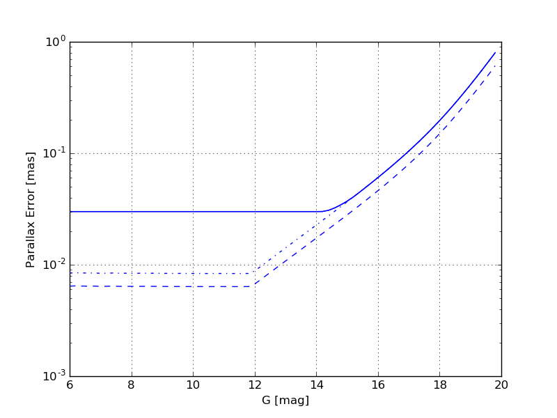
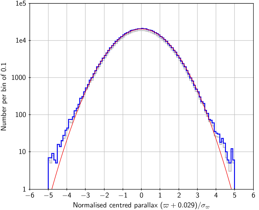
The published parallaxes, and more generally all astrometric parameters, are measured quantities and as such have an associated measurement uncertainty. These uncertainties are published, source per source, and depend mostly on position on the sky as a result of the scanning law and on magnitude. For parallaxes, uncertainties are typically around 0.04 mas for sources brighter than 14 mag, around 0.1 mas for sources with a magnitude around 17, and around 0.7 mas at the faint end, around 20 mag. The astrometric uncertainties provided in Gaia DR2 have been derived from the formal errors computed in the astrometric processing. Unlike for Gaia DR1 , the parallax uncertainties have not been calibrated externally, i.e. they are known, as an ensemble, to be underestimated by 8–12% for faint sources ( mag) outside the Galactic plane and by up to 30% for bright stars ( mag). Based on an assessment of the measured parallaxes of a set of about half a million known quasars, which can be assumed in practice to have zero parallax, the uncertainties are normally distributed with impressive approximation (Fig. 1). However, as is common when taking measurements and especially in such large samples like the Gaia catalogue, there are small numbers of outliers, even up to unrealistically high confidence levels (e.g. at the 100 level).
2.2 Correlations
The parallaxes for each source published in Gaia DR2 have not been derived in isolation, but result from a simultaneous five-parameter fit of an astrometric source model to the data. In Gaia DR2 , only one astrometric source model has been used, that of a single star. This model assumes a uniform, rectilinear space motion relative to the solar system barycentre. The astrometric data in Gaia DR2 thus comprise five astrometric parameters222For a subset of the data, only two parameters (right ascension and declination ) could be determined. with their associated uncertainties, but also ten correlation coefficients between the estimated parameters. It is critical to use the full () covariance matrix when propagating the uncertainties on subsets and/or linear combinations of the astrometric parameters.
As an example, consider the transformation of the measured proper motions and in equatorial coordinates to equivalent values and in galactic coordinates. Following the notation in ESA (1997, Sections 1.2 and 1.5), we have
| (1) |
where the matrix is a rotation matrix that depends on the object’s coordinates and : and . In order to transform the proper-motion errors from the equatorial to the galactic system, we have
| (2) | |||||
| (3) | |||||
| (4) |
where the prime denotes matrix transposition, denotes the Jacobian matrix of the transformation (which for a rotation is the rotation matrix itself), and denotes the variance-covariance matrix. It immediately follows that and depend on the generally non-zero correlation coefficient between the equatorial proper-motion measurements. Neglecting this correlation term can give seriously incorrect results. Some further examples of how error propagation should be handled can be found in, for instance, Brown et al. (1997) and Lindegren et al. (2000). In addition to error propagation, the covariance matrix should also be taken into account when estimating model parameters, for example in chi-square fitting, maximum likelihood estimates, Bayesian analysis, etc. For more details, see Volume 1, Section 1.5 of ESA (1997).
2.3 Systematic errors
Both the design of the spacecraft and the design and implementation of the data processing software and algorithms aim to prevent biases or systematic effects in the astrometry. Systematic errors at low levels nonetheless exist in Gaia DR2 (see Gaia Collaboration et al., 2018a, c). Systematic effects are complicated and largely unknown functions of position on the sky, magnitude, and colour. Although systematic effects are not dealt with in the remainder of this paper, it is important for users to be aware of their presence.
The parallaxes and proper motions in Gaia DR2 may be affected by systematic errors. Although the precise magnitude and distribution of these errors is unknown, they are believed to be limited, on global scales, to 0.1 mas for parallaxes and 0.1 mas yr-1 for proper motions. There is a significant average parallax zero-point shift of about as in the sense Gaia minus external data. This shift has not been corrected for and is present in the published data. Significant spatial correlations between stars, up to 0.04 mas in parallax and 0.07 mas yr-1 in proper motion, exist on both small (1∘) and intermediate (20∘) angular scales. As a result, averaging parallaxes over small regions of the sky, for instance in an open cluster, in the Magellanic Clouds, or in the Galactic Centre, will not reduce the uncertainty on the mean below the mas level.
Unfortunately, there is no simple recipe to account for the systematic errors. The general advice is to proceed with the analysis of the Gaia DR2 data using the uncertainties reported in the catalogue, ideally while modelling systematic effects as part of the analysis, and to keep the systematics in mind when interpreting the results.
2.4 Completeness
As argued in the next sections, a correct estimation requires full knowledge of the survey selection function. Conversely, neglecting the selection function can causes severe biases. Derivation of the selection function is far from trivial, yet estimates have been made for Gaia DR1 (TGAS) by, for instance, Schönrich & Aumer (2017) and Bovy (2017).
This paper does not intend to define the survey selection function. We merely limit ourselves to mentioning a number of features of the Gaia DR2 data that should be properly reflected in the selection function. The Gaia DR2 catalogue is essentially complete between and 17 mag. Although the completeness at the bright end ( in the range 3–7 mag) has improved compared to Gaia DR1 , a fraction of bright stars in this range is still missing in Gaia DR2 . Most stars brighter than 3 mag are missing. In addition, about one out of every five high-proper-motion stars ( arcsec yr-1) is missing. Although the onboard detection threshold at the faint end is equivalent to mag, onboard magnitude estimation errors allow Gaia to see fainter stars, although not at each transit. Gaia DR2 hence extends well beyond mag. However, in dense areas on the sky (above stars deg-2), the effective magnitude limit of the survey can be as bright as 18 mag. The somewhat fuzzy faint-end limit depends on object density (and hence celestial position) in combination with the scan-law coverage underlying the 22 months of data of Gaia DR2 and the filtering on data quality that has been applied prior to publication. This has resulted in some regions on the sky showing artificial source-density fluctuations, for instance reflecting the scan-law pattern. In small, selected regions, gaps are present in the source distribution. These are particularly noticeable near very bright stars. In terms of effective angular resolution, the resolution limit of Gaia DR2 is 0.4 arcsec.
Given the properties of Gaia DR2 summarised above, the interpretation of the data is far from straightforward. This is particularly true when accounting for the incompleteness in any sample drawn from the Gaia Archive. We therefore strongly encourage the users of the data to read the papers and documentation accompanying Gaia DR2 and to carefully consider the warnings given therein before drawing any conclusions from the data.
3 Critical review of the traditional use of parallaxes
We start this section by briefly describing how parallaxes are measured and how the presence of measurement noise leads to the occurrence of zero and negative observed parallaxes. In the rest of the section we review several of the most popular approaches to using measured parallaxes () to estimate distances and other astrophysical parameters. In doing so we will attempt to highlight the intricacies, pitfalls, and problems of these ‘traditional’ approaches.
3.1 Measurement of parallaxes
In simplified form, astrometric measurements (source positions, proper motions, and parallaxes) are made by repeatedly determining the direction to a source on the sky and modelling the change of direction to the source as a function of time as a combination of its motion through space (as reflected in its proper motion and radial velocity) and the motion of the observing platform (earth, Gaia , etc.) around the Sun (as reflected in the parallax of the source). As explained in more detail in Lindegren et al. (2016) and Lindegren et al. (2012), this basic model of the source motion on the sky describes the time-dependent coordinate direction from the observer towards an object outside the solar system as the unit vector
| (5) |
where is the time of observation and is a reference time, both in units of Barycentric Coordinate Time (TCB); , , and are unit vectors pointing in the direction of increasing right ascension, increasing declination, and towards the position of the source, respectively; is the time of observation corrected for the Rømer delay; is the barycentric position of the observer at the time of observation; is the astronomical unit; and denotes normalisation. The components of proper motion along and are respectively and , is the parallax, and is the ‘radial proper motion’ which accounts for the fact that the distance to the star changes as a consequence of its radial motion, which in turn affects the proper motion and parallax. The effect of the radial proper motion is negligibly small in most cases and can be ignored in the present discussion.
The above source model predicts the well-known helix or wave-like pattern for the apparent motion of a typical source on the sky. A fit of this model to noisy observations can lead to negative parallaxes, as illustrated in Fig. 2. We note how in the source model described in Eq. (5) the parallax appears as the factor in front of the barycentric position of the observer, which means that for each source its parallactic motion on the sky will have a sense which reflects the sense of the motion of the observer around the Sun. In the presence of large measurement noise (comparable to the size of the parallax) it is entirely possible that the parallax value estimated for the source model vanishes or becomes negative. This case can be interpreted as the measurement being consistent with the source going ‘the wrong way around’ on the sky, as shown in Fig. 2.
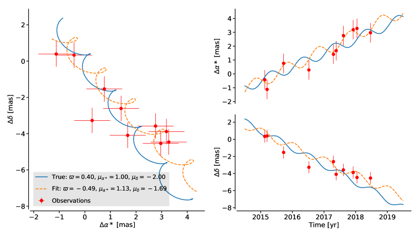
This example is intended to clarify why parallaxes can have non-positive observed values and, more importantly, to convey the message that the parallax is not a direct measurement of the distance to a source. The distance (or any other quantity depending on distance) has to be estimated from the observed parallax (and other relevant information), taking into account the uncertainty in the measurement. A simplified demonstration of how negative parallaxes arise (allowing the reader to reproduce Fig. 2) can be found in the online tutorials accompanying this paper 333%Links␣to␣tutorialhttps://github.com/agabrown/astrometry-inference-tutorials/tree/master/luminosity-calibration/DemoNegativeParallax.ipynb.
3.2 Estimating distance by inverting the parallax
In the absence of measurement uncertainties, the distance to a star can be obtained from its true parallax through , with indicating the true value of the parallax. Thus, naively we could say that the distance to a star can be obtained by inverting the observed parallax, , where now is used to indicate the distance derived from the observed value of the parallax. For this discussion the observed parallax is assumed to be free of systematic measurement errors and to be distributed normally around the true parallax
| (6) |
where indicates the measurement uncertainty on . Blind use of as an estimator of the distance will lead to unphysical results in case the observed parallax is non-positive. Nevertheless, we could still consider the use of the distance estimate for positive values, for instance, a sample where most or all of the observed values are positive or, in the limiting case, where there is a single positive parallax value. In this case, it is crucial to be aware of the statistical properties of the estimate . Given a true distance , what will be the behaviour of ? We can obtain the probability density function (PDF) of from Eq. (6) as
| (7) | |||||
In Fig. 3 we depict for two extreme cases of very low and very high relative uncertainty. The shape of describes what we can expect when using as an estimate of the true distance . The distribution of the figure on the left corresponds to a case with a low fractional parallax uncertainty, defined as . It looks unbiased and symmetrical. Thus, using to estimate the distance in a case like this is relatively safe and would lead to more or less reliable results. However, in spite of its appearance, the figure hides an intrinsic non-Gaussianity that is made evident in the right-hand figure. This second plot corresponds to the case of high fractional parallax uncertainty and the distribution shows several features: first, the mode (the most probable value) does not coincide with the true distance value; second, the distribution is strongly asymmetric; and finally, it presents a long tail towards large values of . For more extreme values of there is a noticeable negative tail to this distribution, corresponding to the negative tail of the observed parallax distribution.
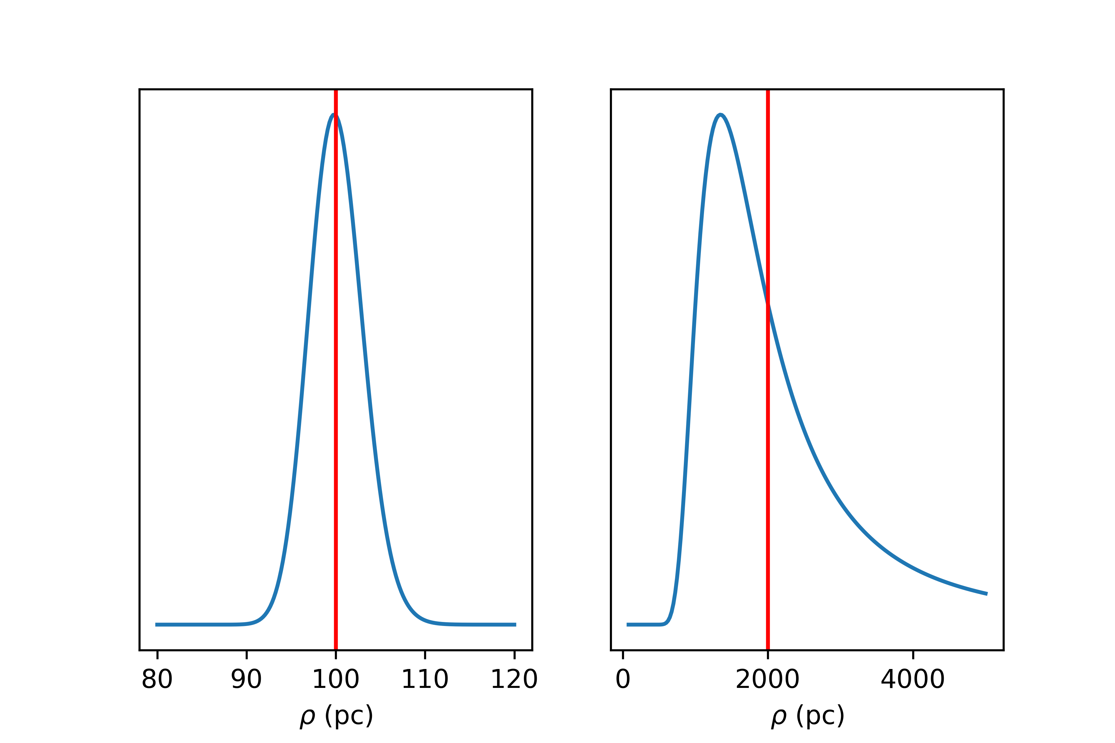
In view of Fig. 3 it is tempting to apply corrections to the estimator based on the value of the fractional parallax uncertainty . Unfortunately, in order to do so we would need to know the true value of the parallax and . Using the apparent fractional uncertainty is not feasible since the denominator in (the true parallax) can be very close to zero, so its distribution has very extended wings and using will often result in gross errors.
Furthermore, reporting a value should always be accompanied by an uncertainty estimate, usually the standard deviation of the estimator, but the standard deviation or the variance is defined in terms of an unknown quantity: . In addition, the long tail shown in the right panel of Fig. 3 makes the estimates of the variance quickly become pathological, as discussed below.
In order to clarify the previous assertions, we recall the classical concept of bias because it plays a central role in the discussion that develops in this section. In statistics, an estimator is said to be biased if its expected value differs from the true value. In our case, we aim to infer the true value of the parallax (or, alternatively, related quantities such as the true distance , absolute magnitude, luminosity, or 3D velocity components), and we aim to infer it from the measured parallax. In the Gaia case this measured parallax will be affected by quasi-Gaussian uncertainties (see Sect. 2.1). In this case the expectation value of the observed parallax coincides with the true value:
| (8) |
where represents the Gaussian probability distribution centred at the true parallax and with a standard deviation . Hence, the observed parallax is an unbiased estimator of the true parallax (under the strong hypothesis that there are no systematic biases associated with the survey and that the errors are normally distributed).
Now, in order to assess the bias of as an estimator of the true distance we need to calculate its expected value:
| (9) |
This bias was approximated by Smith & Eichhorn (1996) (see Sect. 3.4.1) as a function of the fractional parallax uncertainty using a series expansion of the term in the integral and several approximations for the asymptotic regimes of small and large values of , and it indeed shows that the distance estimator is unbiased for vanishingly small values of , but it rapidly becomes significantly biased for values of beyond 0.1. But not only is a biased estimator of the true distance, it is also a high-variance estimator. The reason for this variance explosion is related to the long tail towards large distances illustrated in the right panel of Figs. 3 and 4. Relatively large fractional uncertainties inevitably imply noise excursions in the parallax that result in vanishingly small observed parallaxes and disproportionate distances (and hence an inflation of the variance).
The effects discussed above can be illustrated with the use of simulated data. Figure 4 shows the results of a simulation of objects located between 0.5 and 2kpc where starting from the true distances we have simulated observed parallaxes with a Gaussian uncertainty of mas and then calculated for each object .
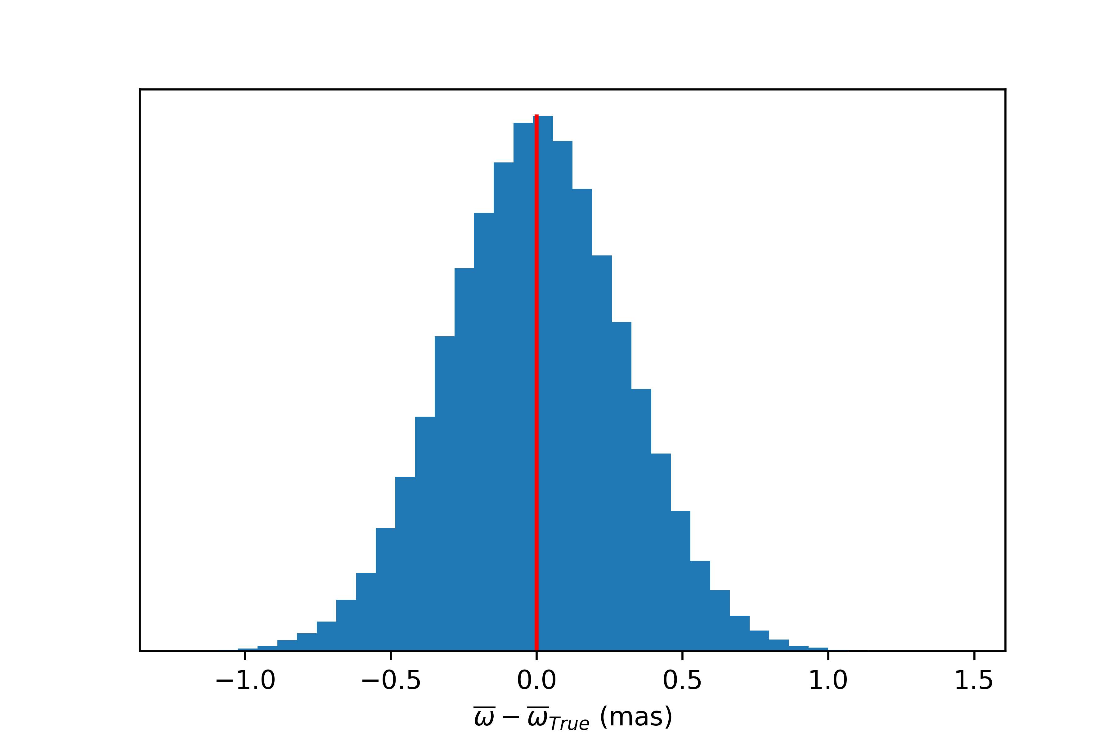
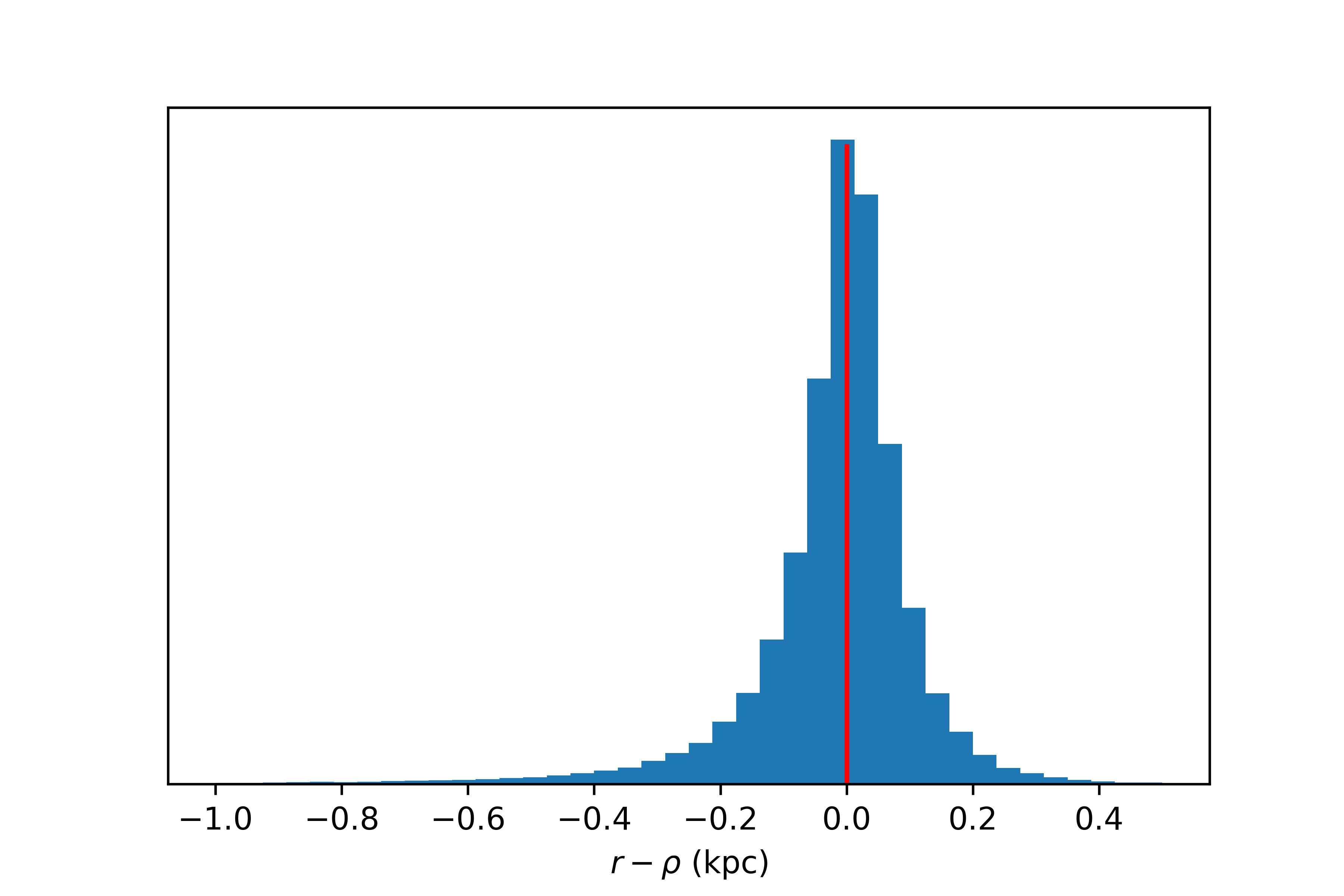
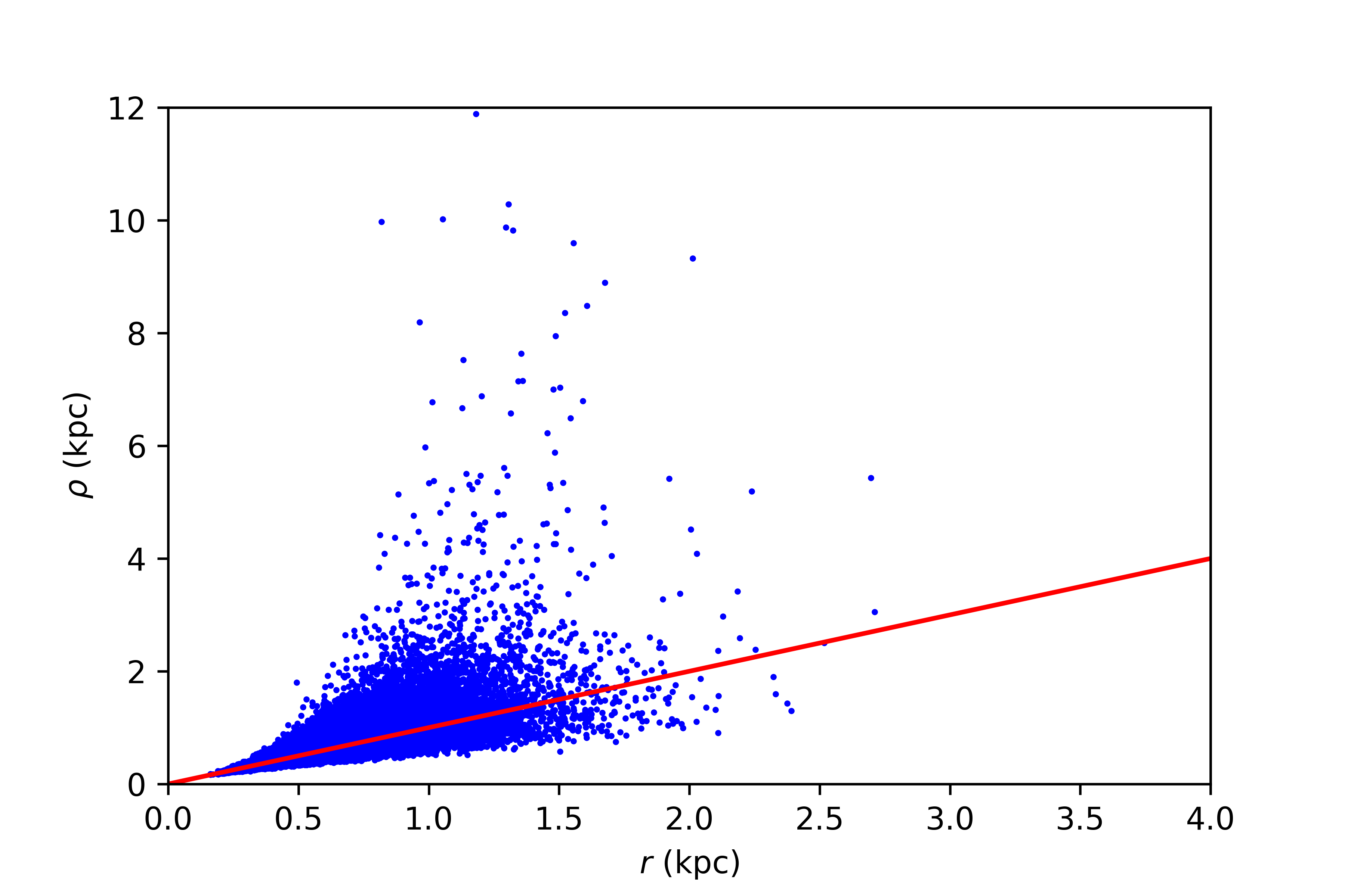
The figure on the left shows that (by construction) the errors in the observed parallaxes are well behaved and perfectly symmetrical (Gaussian), while in the centre figure the errors in the estimation of distances using show a strong asymmetry. The characteristics of these residuals depend on the distribution of true distances and uncertainties. This is more evident in the figure on the right, where the true distance is plotted against ; there is a very prominent tail of overestimated distances and the distribution is asymmetrical around the one-to-one line: the more distant the objects, the more marked the asymmetry. These features are very prominent because we have simulated objects so that the relative errors in parallax are large, but they are present (albeit at a smaller scale) even when the relative errors are small.
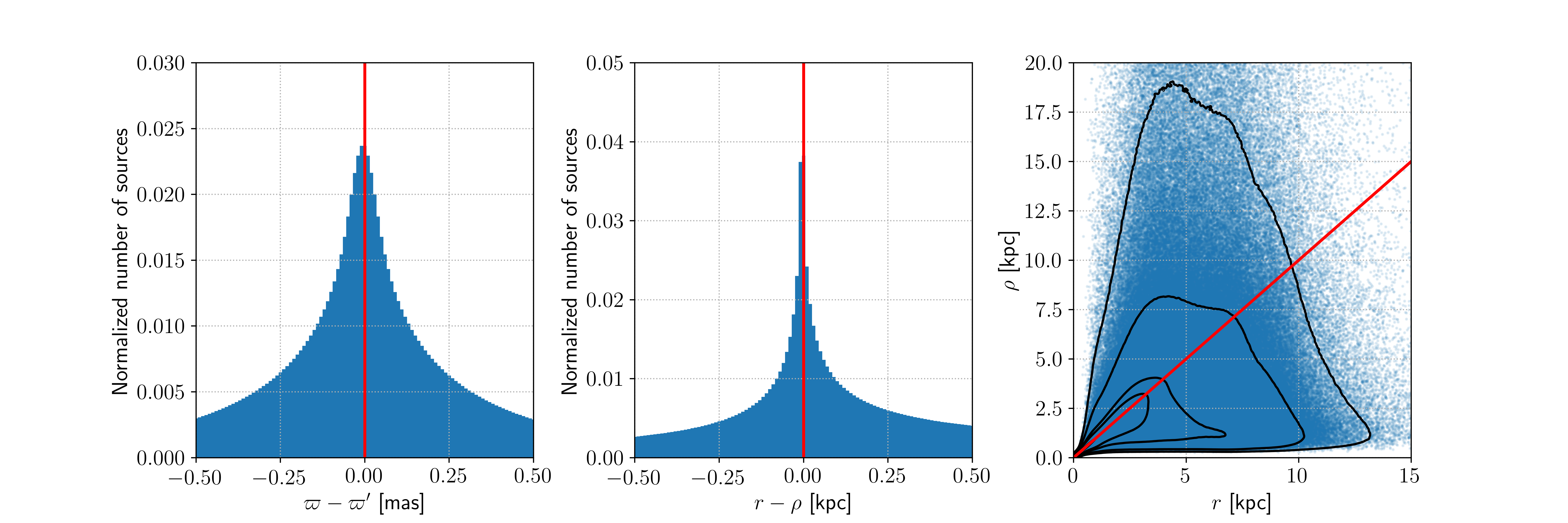
The plots in Fig. 4 correspond to a simple simulation with a mild uncertainty mas. Figure 5 shows the same plots for a realistic simulation of the Gaia DR2 data set. The simulation is described in Appendix A; in this case the errors in parallax follow a realistic model of the Gaia DR2 errors, depicted in Fig. 17.
As a summary, we have seen in previous paragraphs that the naive approach of inverting the observed parallax has significant drawbacks: we are forced to dispose of valuable data (non-positive parallaxes), and as an estimator is biased and has a very high variance.
3.3 Sample truncation
In addition to the potential sources of trouble described in the previous sections, the traditional use of samples of parallaxes includes a practice that tends to aggravate these effects: truncation of the used samples.
As discussed in Sect. 3.1, negative parallaxes are a natural result of the Gaia measurement process (and of astrometry in general). Since inverting negative parallaxes leads to physically meaningless negative distances we are tempted to just get rid of these values and form a ‘clean’ sample. This results in a biased sample, however.
On the one hand, removing the negative parallaxes biases the distribution of this parameter. Consider for instance the case illustrated in Fig. 1 for the quasars from the AllWISE catalogue. These objects have a near zero true parallax, and the distribution of its observed values shown in the figure corresponds to this, with a mean of as, close to zero. However, if we remove the negative parallaxes from this sample, deeming them ‘unphysical’, the mean of the observed values would be significantly positive, about mas. This is completely unrealistic for quasars; in removing the negative parallaxes we have significantly biased the observed parallax set for these objects. With samples of other types of objects with non-zero parallaxes the effect can be smaller, but it will be present.
On the other hand, when by removing negative parallaxes the contents of the sample are no longer representative of the base population from which it has been extracted since stars with large parallaxes are over-represented and stars with small parallaxes are under-represented. This can be clearly illustrated using a simulation. We have generated a sample of simulated stars mimicking the contents of the full Gaia DR2 (see Appendix A) and truncated it by removing the negative parallaxes. In Fig. 6 we can compare the distribution of the true distances of the original (non-truncated) sample and the resulting (truncated) sample; it is clear that after the removal of negative parallaxes we have favoured the stars at short distances (large parallaxes) with respect to the stars at large distances (small parallaxes). The spatial distribution of the sample has thus been altered, and may therefore bias any analysis based on it.
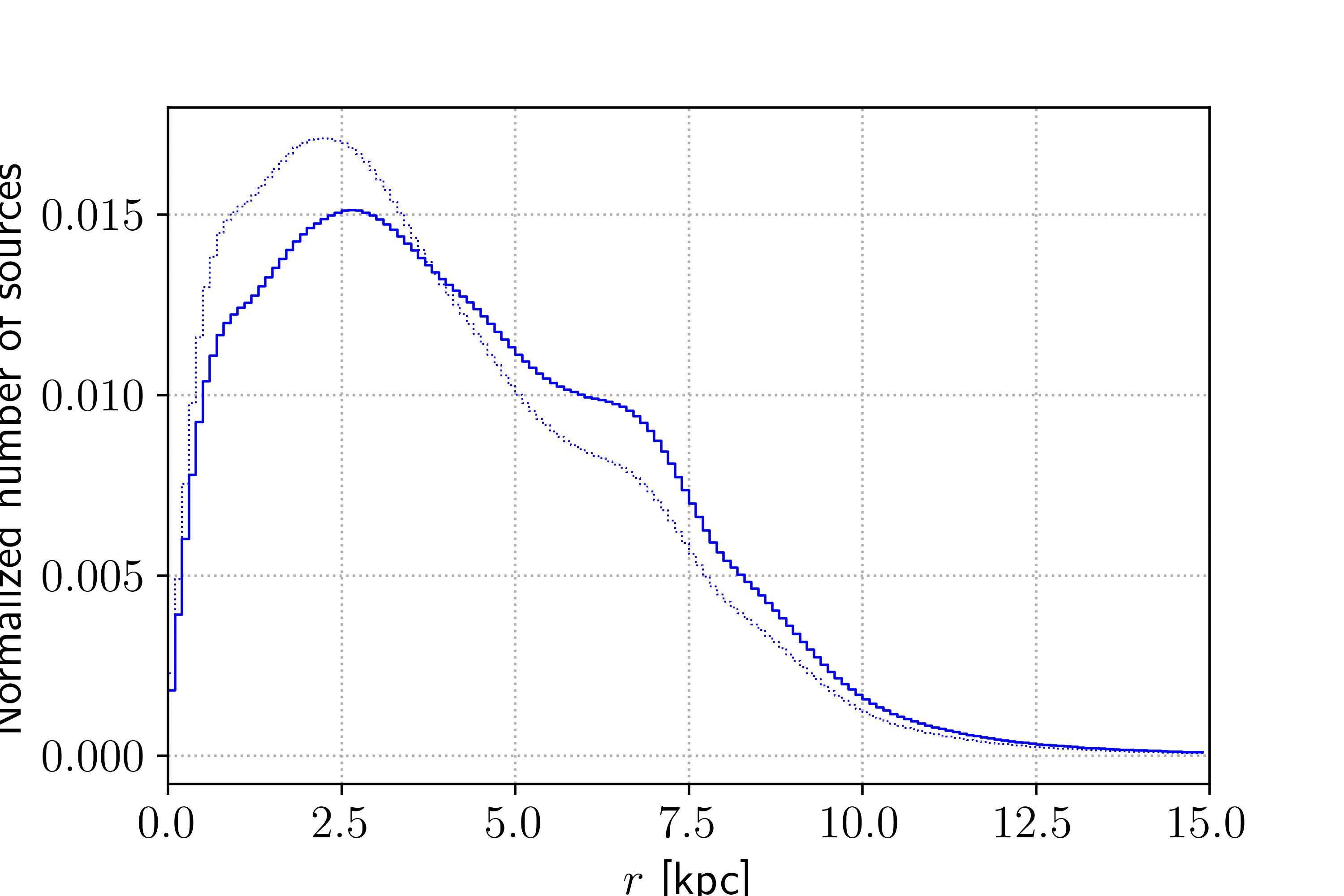
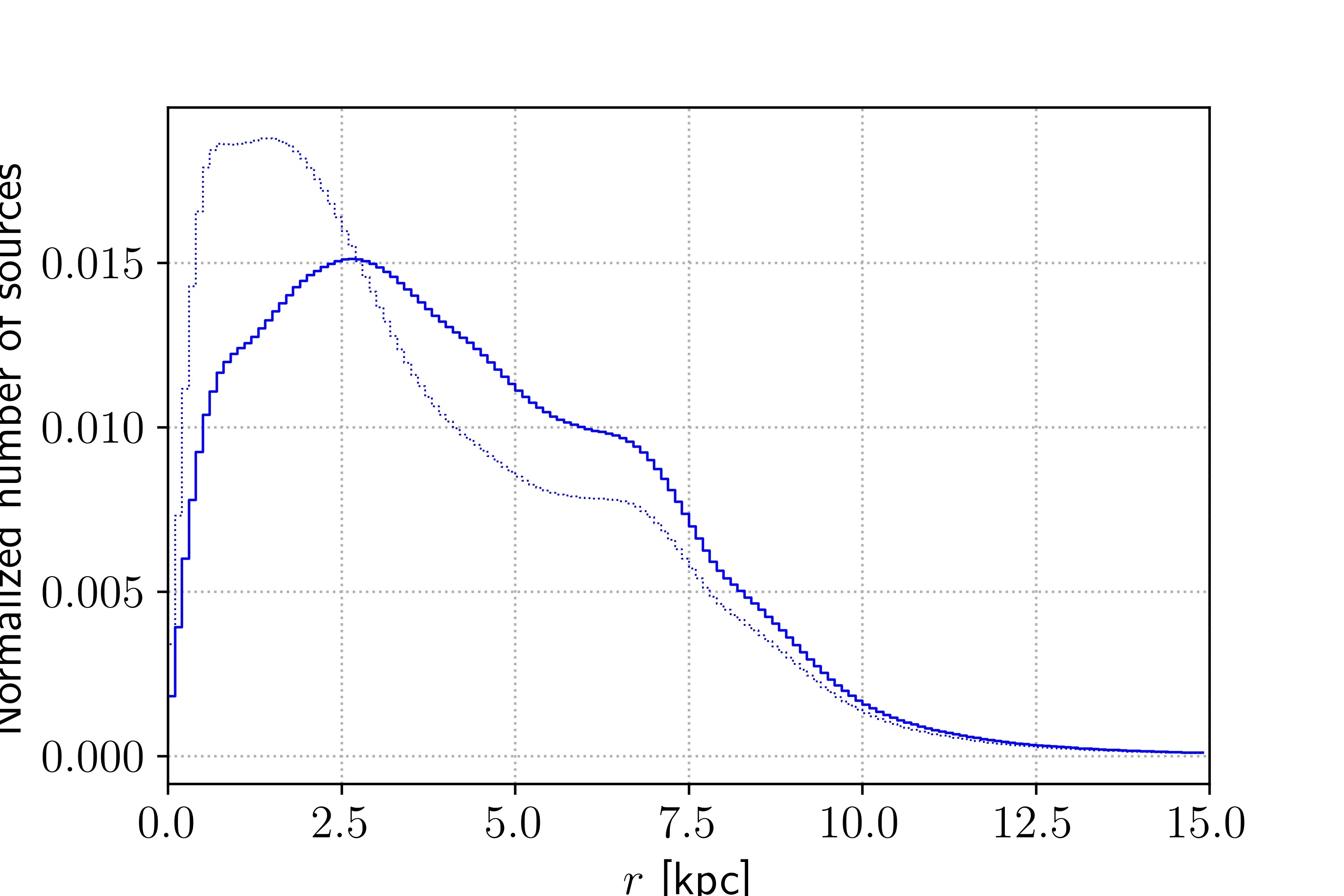
A stronger version of truncation that has traditionally been applied is to remove not only negative parallaxes, but also all the parallaxes with a relative error above a given threshold , selecting . This selection tends to favour the removal of stars with small parallaxes. The effect is similar to the previous case, but more accentuated as can be seen in Fig. 7. Again, stars at short distances are favoured in the sample with respect to distant stars.
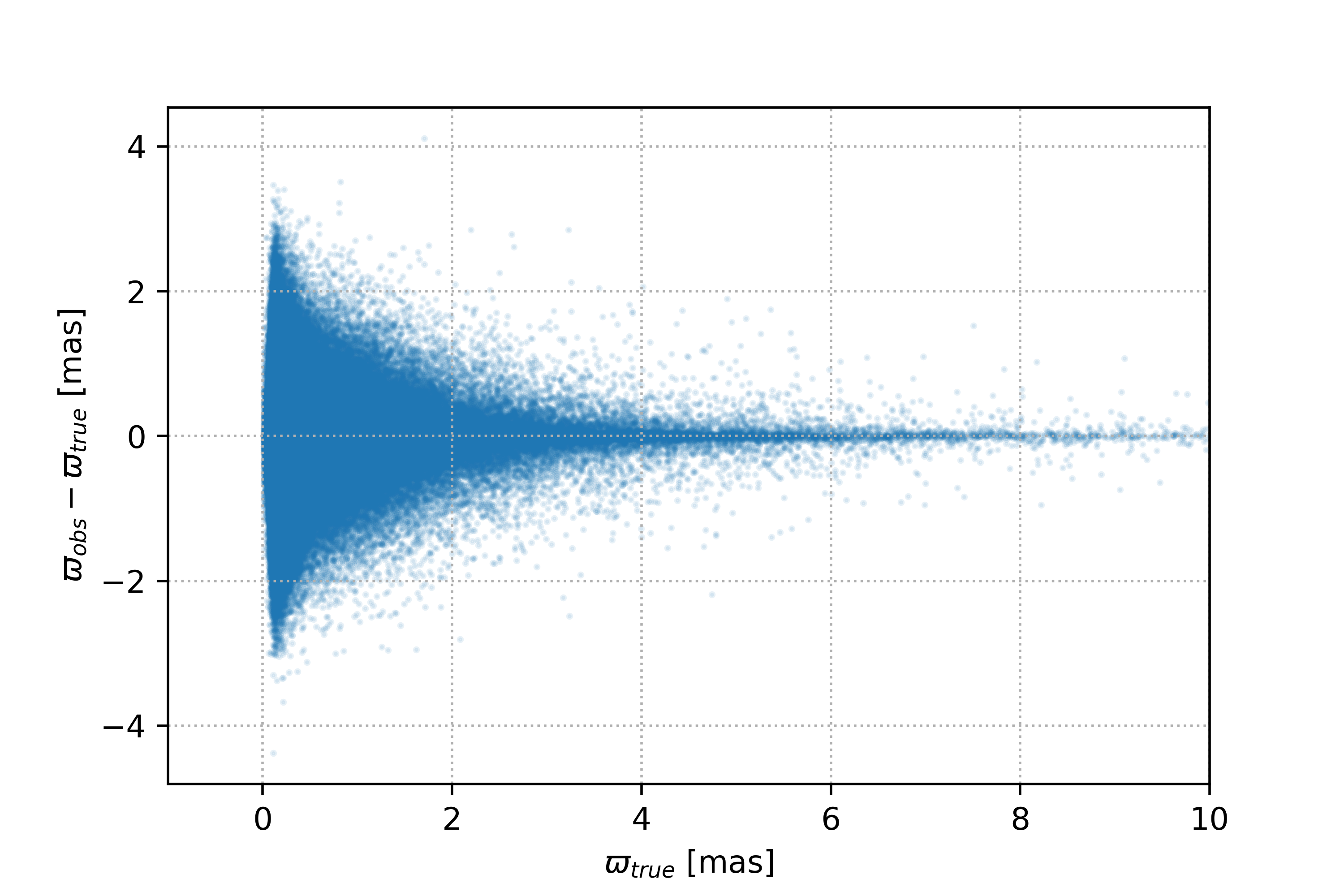
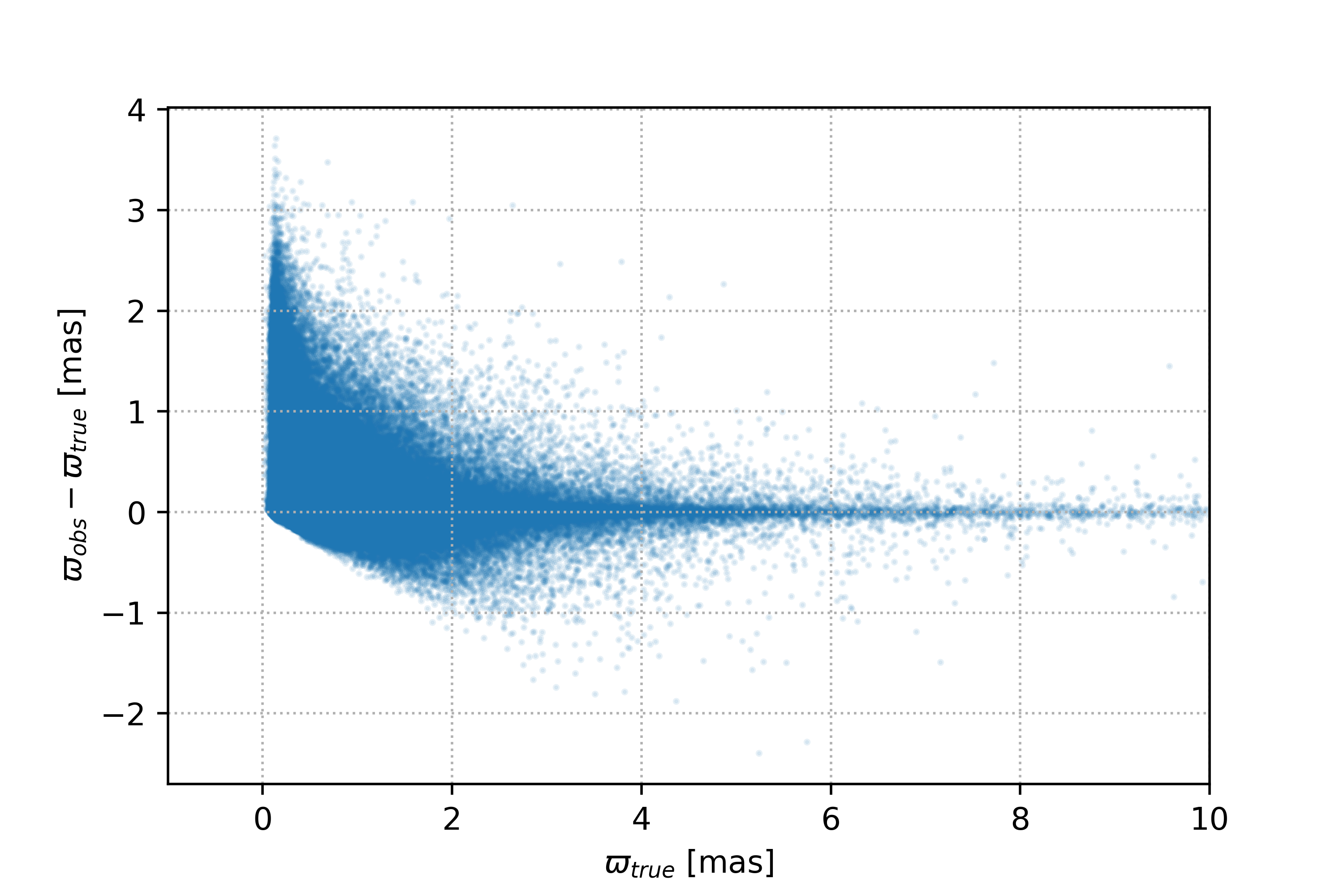
Even worse, as in the previous case the truncation not only makes the distribution of true distances unrepresentative, but it also biases the distribution of observed parallaxes: stars with positive errors (making the observed parallax larger than the true one) tend to be less removed than stars with negative errors (making the observed parallax smaller than the true one). By favouring positive errors with respect to negative errors, we are also biasing the overall distribution of parallaxes. Figure 8 depicts this effect. The plots show the difference as a function of . We can see in the middle and bottom figures how the removal of objects is non-symmetrical around the zero line, so that the overall distribution of becomes biased. From an almost zero bias for the full sample (as expected from Gaia in absence of systematics) we go to significant biases once we introduce the truncation, and the bias is dependent of the cut value we introduce.
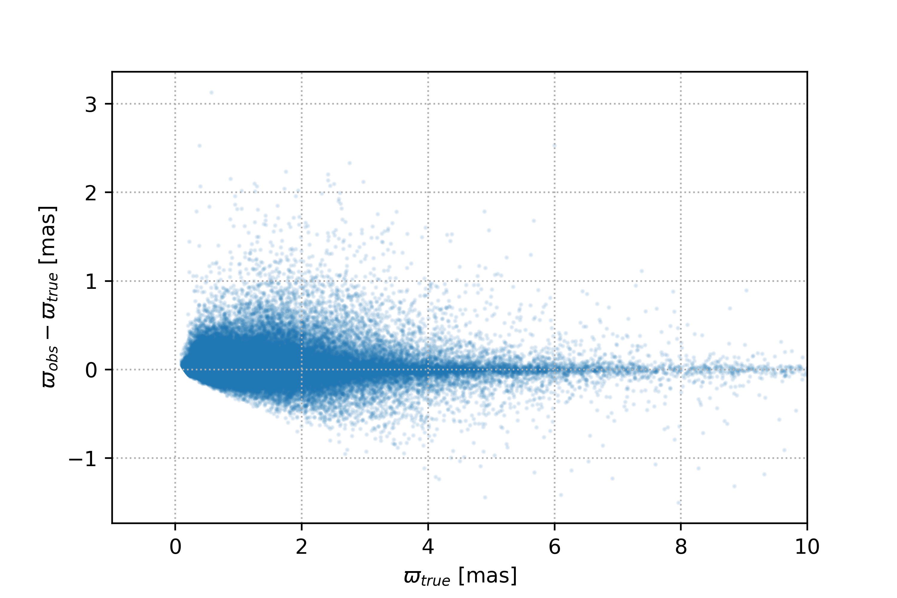
Furthermore, in Gaia the parallax uncertainties vary with the object magnitude, being larger for faint stars (see Fig. 17). Therefore, a threshold on the relative error will favour bright stars over the faint ones, adding to the above described biases.
Another type of truncation that has been traditionally applied is to introduce limits in the observed parallax. The effects of such a limit are closely related to the Lutz–Kelker bias discussed in Sect. 3.4.2. Suffice it here to illustrate the effect with a specific example on a Gaia DR2 -like sample. If we take the full sample and remove stars with mas we could imagine that we are roughly removing objects further away than 5 kpc. However, the net result is depicted in Fig. 9 where we can see that instead of the distribution of true distances of the complete sample up to 5 kpc (solid line) we get a distribution with a lack of closer stars and a long tail of stars with greater distances. A larger limit in parallax (shorter limiting distance) will produce a less prominent effect since the relative errors in the parallax will be smaller, but the bias will be nonetheless present.
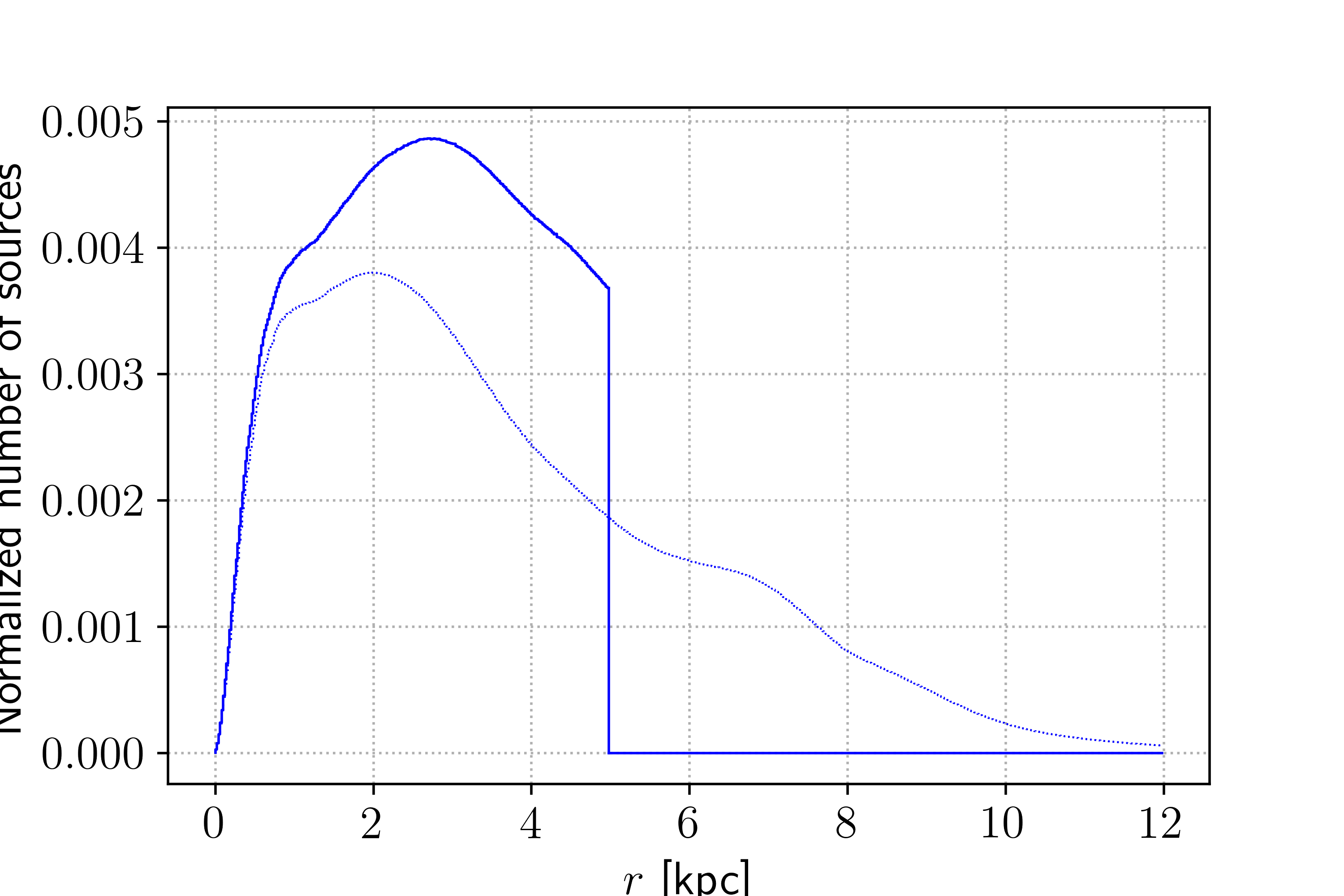
In conclusion, our advice to readers is to avoid introducing truncations when using Gaia data since, as illustrated above, they can strongly affect the properties of the sample and therefore affect the data analysis. If truncation is unavoidable it should be included in the Bayesian modelling of the overall problem (see Sect. 4.3).
3.4 Corrections and transformations
In this section, we review proposals in the literature for the use of parallaxes to estimate distances. In general they take the form of ‘remedies’ to correct one or another problem on this use. Here we explain why these remedies cannot be recommended.
3.4.1 The Smith–Eichhorn correction
Smith & Eichhorn (1996) attempt to compensate for the bias introduced by the naive inversion of the observed parallax (and the associated variance problem) in two different ways. The first involves transforming the measured parallaxes into a pseudo-parallax according to
| (10) |
where and is an adjustable constant. The qualitative effect of the transformation is to map negative parallaxes into the positive semi-axis and to increase the value of small parallaxes until it asymptotically converges to the measured value for large . For , and the pseudo-parallax value has the undesirable property of depending on the choice of and on the parallax uncertainty. Thus, even in the case of a small parallax measurement with a relatively small fractional parallax uncertainty (e.g. ), we substitute a perfectly useful and valuable measurement by an arbitrary value of .
The Smith–Eichhorn transformation is an arbitrary (and rather convolved) choice amongst many such transformations that can reduce the bias for certain particular situations. Both the analytical expression and the choice of constants and are the result of an unspecified trial-and-error procedure, the applicability of which is unclear. Furthermore, as stated by the authors, they introduced a new bias because the transformed parallax is always larger than the measured parallax. This new bias has no physical interpretation because it is the result of an ad hoc choice for the analytical expression in Eq. (10). It is designed to reduce the bias, but it does so by substituting perfectly reasonable direct measurements (negative and small parallaxes) that we can interpret and use for inference, by constructed values arising from the choice.
3.4.2 The Lutz–Kelker correction
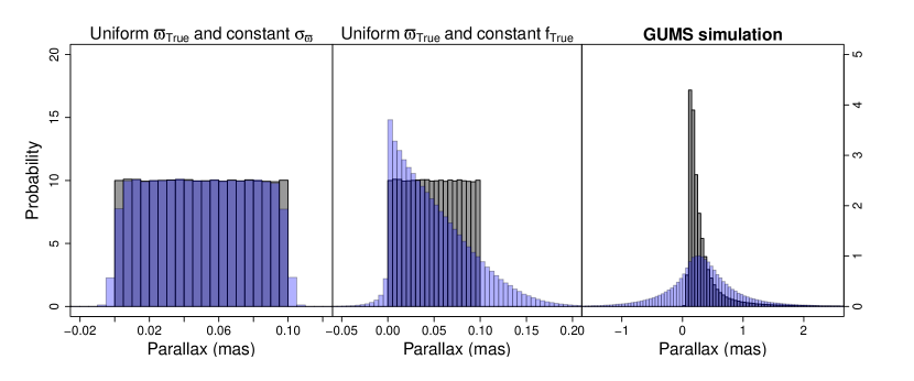
Lutz & Kelker (1973) realised that the spatial distribution of sources around the observer together with the unavoidable observational errors and a truncation of the sample on the value of the observed parallax result in systematic biases in the average parallax of certain stellar samples. The bias described by Lutz & Kelker (1973) is a manifestation of the truncation biases described above and can be understood if we look at a few very simple examples. First, let us imagine a density of sources around the observer such that the distribution of true parallaxes is constant in a given interval and zero outside. Let us also imagine that the observation uncertainty is constant and equal to 0.3 mas. The left panel of Fig. 10 shows the distribution of true and observed parallaxes for a simulation of such a situation and sources. We see that the observed parallaxes are also approximately uniform and the departures from uniformity appear near the edges. For a given bin of intermediate parallax we have as many sources contaminating from neighbouring bins as we have sources lost to other bins due to the observational uncertainties, and the result is a negligible net flux.
In the middle panel we show the same histograms except that instead of a constant parallax uncertainty, we use a constant value of the fractional parallax uncertainty . This is still an unrealistic situation because the distribution of true parallaxes is not uniform and also because a constant implies that larger parallaxes are characterised by larger uncertainties. However, it helps us to illustrate that even in the case of uniform true parallaxes we may have a non-zero net flux of sources between different parallax bins depending on the distribution of parallax uncertainties. In this case, noise shifts the value of large parallaxes more than that of smaller parallaxes (because of the constant value of ), so larger parallaxes get more scattered, thus suppressing the distribution more at large parallaxes.
Finally, the right panel shows the same plot for a realistic distribution of distances from a Gaia Universe Model Snapshot (GUMS) sample (see Appendix A for a full description). We see that the effect of a realistic non-uniform distribution of parallaxes and parallax uncertainties results in a net flux in the opposite direction (smaller true parallaxes become more suppressed and larger parallax bins are enhanced; in both cases, the bins of negative parallaxes become populated). This is the root of the Lutz–Kelker bias. It is important to distinguish between the Lutz–Kelker bias and the Lutz–Kelker correction. The Lutz–Kelker bias is the negative difference for any realistic sample between the average true parallax and the average measured parallax (i.e. the average true parallax is smaller than the average measured parallax). This bias has been known at least since the work of Trumpler & Weaver (1953), although it was already discussed in a context different from parallaxes as early as Eddington (1913). The Lutz–Kelker correction presented in Lutz & Kelker (1973) and discussed below is an attempt to remedy this bias based on a series of assumptions.
In the case of Gaussian uncertainties such as those described in Eq. (6) it is evident that the probability of measuring a value of the parallax greater than the true parallax . The same value holds for the probability that because the Gaussian distribution is symmetrical with respect to the true value of the parallax. This is also true for the joint probability of and ,
| (11) |
where is the region of the plane where .
However, the probability distribution of the true parallax given the observed parallax does not fulfil this seemingly desirable property of probability mass equipartition at the point. We can write the latter probability as
| (12) |
using the product rule of probability. In the context of inferring the true parallax from the observed one, Eq. (12) is the well-known Bayes’ theorem, where the left-hand side is the posterior probability, is the likelihood, is the prior, and is the evidence. For most realistic prior distributions , neither the median nor the mode or the mean of the posterior in Eq. (12) is at . Let us take for example a uniform volume density of sources out to a certain distance limit. In such a distribution the number of sources in a spherical shell of infinitesimal width at a distance scales as , as does the probability distribution of the distances. Since
| (13) |
the probability distribution for the true parallax in such a truncated constant volume density scenario is proportional to
| (14) |
out to the truncation radius. Hence, for Gaussian distributed uncertainties we can write as
| (15) |
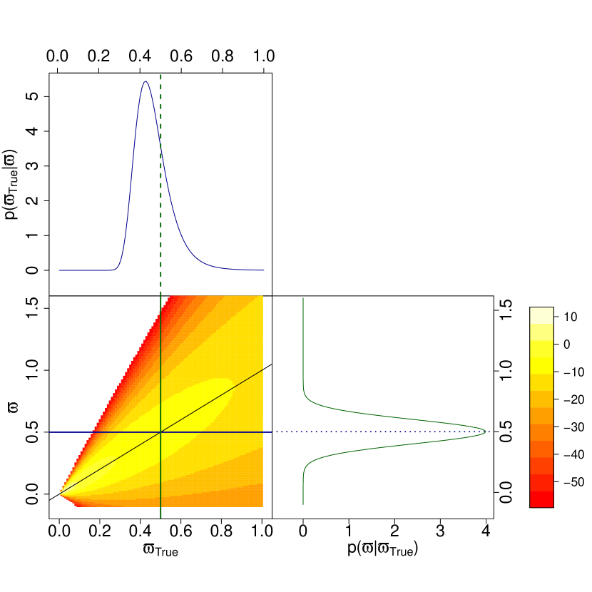
The joint distribution (i.e. the non-normalised posterior, plotted as a 2D function of data and parameter ) for this particular case of truncated uniform stellar volume densities is depicted in Fig. 11 together with the conditional distributions for particular values of and . It shows graphically the symmetry of the probability distribution (with respect to ) and the bias and asymmetry of .
Lutz & Kelker (1973) obtain Eq. (15) in their Sect. ii under the assumption of uniform stellar volume densities and constant fractional parallax uncertainties (constant ). They discuss several distributions for different values of the ratio . In their Sect. iii they use the expected value of the true parallax given by the distribution in Eq. (15) to infer the expected value of the difference between the true absolute magnitude and the value obtained with the naive inversion of the observed parallax. The expected value of this absolute magnitude error is derived and tabulated for the distribution as a function of the fractional parallax uncertainty . This so-called Lutz–Kelker correction is often applied to stellar samples that do not fulfil the assumptions under which it was derived because the stellar volume density is far from uniform at scales larger than a few tens of parsecs and the samples to which the correction is applied are never characterised by a unique value of .
3.5 Astrometry-based luminosity
An obvious way to avoid the problems associated with the naive inversion of observed parallaxes (see Sect. 3.4.1) is to remain in the space of parallaxes (as opposed to that of distances) insofar as this is possible. One example of this approach is the astrometry-based luminosity (ABL) method (Arenou & Luri, 1999) originating from Malmquist (1920). The ABL method consists in substituting the absolute magnitudes by a proxy that is linearly dependent on the parallax. The original proposal was
| (16) |
and has been recently used to obtain maximum likelihood estimates of the period-luminosity relation coefficients for Cepheids and RR Lyrae stars (Gaia Collaboration et al., 2017a), and to improve the Gaia parallax uncertainties using deconvolved colour-magnitude diagrams as prior (Anderson et al., 2017). The new astrometry-based luminosity depends linearly on the parallax, and thus its uncertainty can be expected to have an approximately Gaussian distribution if the fractional uncertainty of the apparent magnitude is negligible. This is more often the case than for fractional parallax uncertainties and is in general a good approximation.
Unfortunately, the astrometry-based luminosity can only be applied to the study of the luminosity and can do nothing for the analysis of spatial distributions where distances or tangential velocities are inevitable ingredients.
4 Recommendations for using astrometric data
In this section we provide specific advice on the use of astrometric data in astronomical data analysis. Although the focus is on the use of Gaia data, many of the recommendations hold for the analysis of astrometric data in general. To illustrate the recommendations we also provide a small number of worked examples, ranging from very basic demonstrations of the issues mentioned in Sect. 3 to full Bayesian analyses. Some of these examples are available in the Gaia archive tutorial described in Sect. 5.
4.1 Using Gaia astrometric data: how to proceed?
The fundamental quantity sought when measuring a stellar parallax is the distance to the star in question. However, as discussed in the previous sections the quantity of interest has a non-linear relation to the measurement, , and is constrained to be positive, while the measured parallax can be zero or even negative. Starting from a measured parallax which is normally distributed about the true parallax, this leads to a probability density for the simple distance estimator (see Sect. 3) for which the moments are defined in terms of unknown quantities. This means we cannot calculate the variance of the estimator or the size of a possible bias, which renders the estimator useless from the statistical point of view.
Our first and main recommendation is thus to always treat the derivation of (astro-)physical parameters from astrometric data, in particular when parallaxes are involved, as an inference problem which should preferably be handled with a full Bayesian approach.
4.1.1 Bayesian inference of distances from parallaxes
The Bayesian approach to inference involves estimating a PDF over the quantity of interest given the observables. In this case we want to estimate the distance, , given the parallax, . A fuller treatment of this problem has been given in Bailer-Jones (2015), so only a brief summary will be given here. Using Bayes’ theorem we can write the posterior as
| (17) |
Formally, everything is also conditioned on the parallax uncertainty, , and any relevant constraints or assumptions, but symbols for these are omitted for brevity. The quantity is the likelihood from Eq. (12). The prior, , incorporates our assumptions and is a normalisation constant.
In addition to the likelihood, there are two important choices which must be made to estimate a distance: the choice of prior and the choice of estimator. We will first focus on the former, and start discussing the simplest prior: the uniform unbounded prior. With a uniform boundless (and thus improper) prior on distances the posterior is proportional to the likelihood, and if we choose the mode of the posterior as our estimator, then the solution is mathematically equivalent to maximising the likelihood. However, a boundless uniform prior permits negative distances, which are non-physical, so we should at least truncate it to exclude these values.
The more measurements we have, or the more precise the measurements are, the narrower the likelihood and the lower the impact of the prior should be on the posterior. It turns out, however, that with the unbounded uniform prior the posterior is improper, i.e. it is not normalisable. Consequently, the mean and median are not defined. The only point estimator is the mode, i.e. (the standard deviation and the other quantiles are likewise undefined), which is rather restrictive. Finally, this Bayesian distance estimate defined for an unbounded uniform prior reduces to the maximum likelihood estimate and coincides with the naive inversion discussed in Sect. 3.2. The posterior is ill-defined for the unbounded uniform prior for parallaxes. This prior describes an unrealistic situation where the observer is placed at the centre of a distribution of sources that is spherically symmetric and the volume density of which decreases sharply with distance.
The solution to these problems (non-physical distances, improper posterior) is to use a more appropriate prior. The properties of various priors and estimators have been studied by Bailer-Jones (2015) and Astraatmadja & Bailer-Jones (2016b). The latter makes a detailed study using a Milky Way model for a prior, and also investigates how the estimates change when the Gaia photometric measurements are used in addition to the parallax. One of the least informative priors we can use is the exponentially decreasing space density prior:
| (18) |
For distances this corresponds to a constant space density of stars, with the probability dropping exponentially at distances much larger than the mode (which is at ). Examples of the shape of the posterior for parallaxes of different precisions are shown in Bailer-Jones (2015) and Astraatmadja & Bailer-Jones (2016b).
The posterior obtained for the prior defined in Eq. (18) is normalised and thus, we have a choice of point estimators (mean, median, or mode). Also, the distribution is asymmetric, and two quantiles (5% and 95%) rather than the standard deviation are recommended to summarise the uncertainty in the point estimate. The median, as a point estimate, is guaranteed to lie between these quantiles. Astraatmadja & Bailer-Jones (2016b) used this prior, as well as a Milky Way prior, to infer distances for the two million TGAS stars in the first Gaia data release. The behaviour of the estimates derived from the exponentially decreasing space density prior can be explored using the interactive tool available in the tutorial described in Sect. 5.1.
In general, the introduction of reasonable prior probabilities accounts for the Lutz–Kelker bias, although the inevitable mismatch between the true distribution of parallaxes and the prior used will result in less accurate inferences. In any case, the advantage with respect to the methods discussed in Sect. 3 is clear: i) we do not need to tabulate corrections for each prior assuming constant ; ii) we do not need to dispose of non-positive parallaxes; iii) we obtain a proper full posterior distribution with well-defined moments and credible intervals; iv) even simple priors such as the exponential decreasing volume density will improve our estimates with respect to the unrealistic prior underlying the maximum likelihood solution ; and finally, v) we obtain estimators that degrade gracefully as the data quality degrades, and with credible intervals that grow with the observational uncertainties until they reach the typical scales of the prior when the observations are non-informative. These advantages come at the expense of an inference that is more computationally demanding in general (as it requires obtaining the posterior and its summary statistics if needed), the need for a thoughtful choice of a prior distribution, and the analysis of the influence of the prior on the inference results.
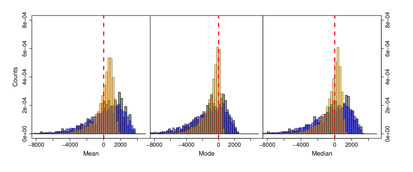
Figure 12 shows the distribution of means (left), modes (centre), and medians (right) of the posteriors inferred for a simulation of sources drawn from an exponentially decreasing space density distribution. This simulation represents the unlikely case where the prior is a perfect representation of the true distribution.
From a Bayesian perspective the full posterior PDF is the final result of our inference if we only use parallax measurements to infer the distance (see below), and further analyses should make use of it as a whole. This is our recommendation in general: avoid expectations and summaries of the posterior. However, it is often useful to compute summary statistics such as the mean (expectation), median, mode, quantiles, etc., to have an approximate idea of the distribution, but we should not use these summaries for further inference, for example to estimate absolute magnitudes, Cartesian velocities, etc. We recommend inferring the full posterior distributions for these derived quantities using the posterior of the true parallax or of the distance, or using the same Bayesian scheme as for the true parallax as explained in Sect. 4.2. In Fig. 13 we show the values of the mean (left), mode (centre), and median (right) that we would obtain from a set of simulated observations of a star at 100 parsecs with . We assume a Gaussian distribution of the observations around the true parallax. The posterior distribution is inferred using Eq. (17) and two priors: a uniform volume density of sources truncated at 1 kpc (results in grey) and a uniform density of sources multiplied by an exponential decay of length scale 200 pc as defined in Eq. (18) (in blue). The expectation values of the histograms are shown as dashed lines of the same colour, with the true value (100 pc) shown as a red dashed line. We see in general that i) the truncation has the effect of increasing the number of overestimated distances; ii) the three estimators are biased towards larger distances (smaller parallaxes), but the expectation of the mode is significantly closer to the true value; and iii) the abrupt truncation of the prior results in a spurious peak of modes at the truncation distance as already discussed in Bailer-Jones (2015).
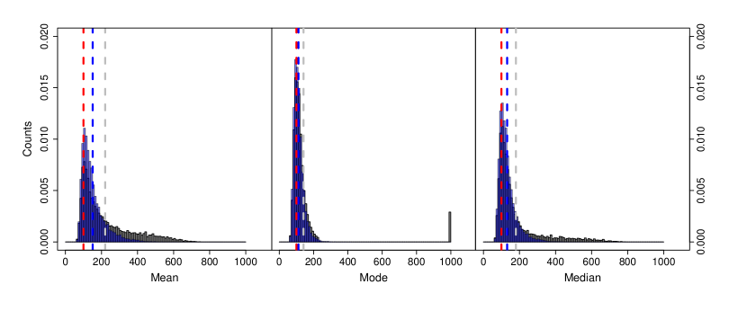
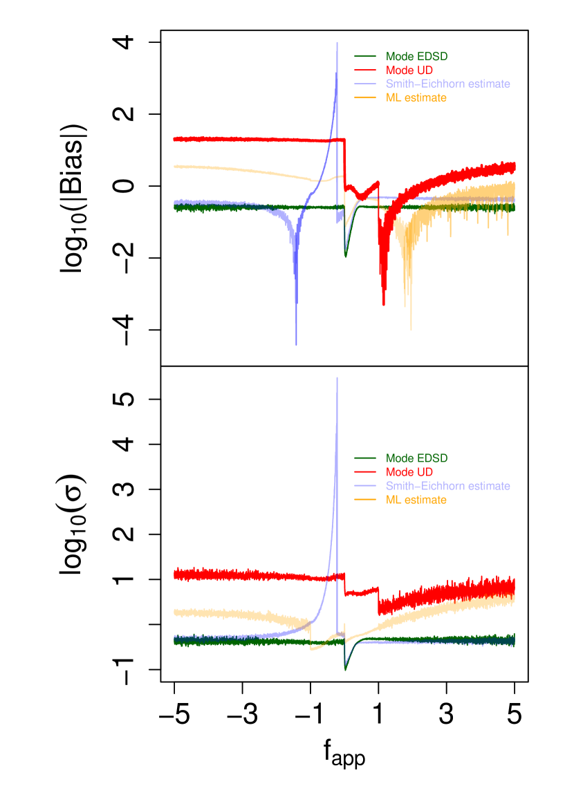
Figure 14 and Table 1 show a comparison of the absolute value of the empirical bias and standard deviation associated with some distance estimators discussed in this paper as a function of the measured fractional uncertainty in the parallax. We chose the measured value even though it is a very poor and non-robust estimator because, as stated in Sect. 3.2, we never have access to the true fractional parallax uncertainty. This figure shows the results obtained for sources in the Gaia DR2 simulation described in Appendix A for the maximum likelihood estimate with and without the Smith–Eichhorn correction, and for the mode estimates based on the posterior distribution for two priors (a uniform distance prior, UD, with maximum distance kpc, and an exponentially decreasing space density prior, EDSD, with kpc), neither of which matches the true distribution of sources in the simulation. Only the mode of the posteriors is plotted (but not the mean or the median) for the sake of clarity. The conclusions described next are only valid under the conditions of the exercise and are provided as a demonstration of the caveats and problems described in previous sections, not as a recommendation of the mode of the posterior inferred under the EDSD prior as an estimator. At the risk of repeating ourselves, we emphasise the need to adopt priors adapted to the inference problem at hand. Also, the conclusions only hold for the used simulation (where we generate the true distances and hence can calculate the bias and standard deviation) and need not be representative of the true performance for the real Gaia data set. They can be summarised as follows:
-
•
the mode of the EDSD prior shows the smallest bias and standard deviation in practically the entire range of estimated fractional parallax uncertainties (in particular, everywhere beyond the range of represented in the plot);
-
•
the Smith–Eichhorn estimate shows pathological biases and standard deviations in the vicinity of the supposedly best-quality measurements at . Away from this region, it provides the next less biased estimates (averaged over bins of ) after the mode of the EDSD posterior;
| Summary | Range | EDSD | UD | SE | ML |
|---|---|---|---|---|---|
| Bias | (-1,1) | -0.2 | 9.7 | 34.2 | -0.95 |
| (-5,5) | -0.3 | 10.7 | -0.34 | -1.2 | |
| (-50,50) | -0.3 | 16.2 | -0.4 | -3.8 | |
| Std. Deviation | (-1,1) | 0.4 | 8.0 | 685.8 | 0.5 |
| (-5,5) | 0.4 | 8.4 | 0.5 | 1.95 | |
| (-50,50) | 0.4 | 10.6 | 0.4 | 17.1 |
4.1.2 Bayesian inference of distances from parallaxes and complementary information
The methodology recommended in the previous paragraphs is useful when we only have observed parallaxes to infer distances. There are, however, common situations in astronomy where the parallaxes are only one of many observables, and distances are not the final goal of the inference problem but a means to achieve it. In this context, we recommend an extension of the classical Bayesian inference methods described in the previous section. These problems are characterised by a set of observables and associated uncertainties (that include but are not restricted to parallaxes) and a series of parameters (the values of which are unknown a priori) with complex interdependence relationships amongst them. Some of these parameters will be the ultimate goal of the inference process. Other parameters do play an important role, but we are not interested in their particular values, and we call them nuisance parameters, following the literature. For example, in determining the shape of a stellar association, the individual stellar distances are not relevant by themselves, but only insomuch as we need them to achieve our objective. We show below how we deal with the nuisance parameters. The interested reader can find applications of the methodology described in this section to inferring the coefficients of period-luminosity relations in Gaia Collaboration et al. (2017a) and Sesar et al. (2017). Also, the same methodology (a hierarchical Bayesian model) is applied in Hawkins et al. (2017) where the constraint on the distances comes not from a period-luminosity relation, but from the relatively small dispersion of the absolute magnitudes and colour indices of red clump stars. A last example of this methodology can be found in Leistedt & Hogg (2017b) where the constraint comes from modelling the colour-magnitude diagram.
Just as in the previous section where we aimed at estimating distances from parallaxes alone, the two key elements in this case are the definitions of a likelihood and a prior. The likelihood represents the probability distribution of the observables given the model parameters. Typically, the likelihood is based on a generative or forward model for the data. Such models predict the data from our assumptions about the physical process that generates the true values (i.e. the distribution of stars in space) and our knowledge of the measurement process (e.g. justifying the assumption of a normal distribution of the observed parallax around its true value). Forward models can be used to generate arbitrarily large synthetic data sets for a given set of the parameters. In this case, however, where we are concerned with several types of measurements that depend on parameters other than the distance, the likelihood term will be in general more complex than in Sect. 4.1.1 and may include probabilistic dependencies between the parameters. The term hierarchical or multi-level model is often used to refer to this kind of model.
Let us illustrate the concept of hierarchical models with a simple extension of the Bayesian model described in Sect. 4.1.1, where instead of assuming a fixed value of the prior length scale in Eq. (18), we make it another parameter of the model and try to infer it. Let us further assume that we have a set of parallax measurements , one for each of a sample of stars. In this case, the likelihood can be written as
| (19) | |||||
where is the true unknown distance to the th star. We note that very often the measured parallaxes are assumed independent, and thus is written as the product . This is incorrect in general for Gaia parallaxes because the parallax measurements are not independent. As described in Gaia Collaboration et al. (2018c) and Sect. 2 of this paper, there are regional correlations amongst them (see Sect. 4.3), but for the sake of simplicity let us assume the sample of measurements is spread all over the celestial sphere such that the correlations average out and can be neglected. Hence, we write
| (20) |
Under the assumption of Gaussian uncertainties, the first term in the product is given by Eq. (6), while the second is given by Eq. (18).
This likelihood can be represented by a simple directed graph (see Fig. 15) that provides information about the conditional dependencies amongst the parameters. The shaded nodes represent the observations, the open circles represent model parameters, and the small black circles at the origin of the arrows represent model constants. The arrows denote conditional dependence relations, and the plate notation indicates repetition over the measurements .
The next key element is, as in Sect. 4.1.1, the prior. According to Fig. 15, the only parameter that needs a prior specification is the one without a parent node: . The rest of the arcs in the graph are defined in the likelihood term (Eq. (20)). If the sample of stars were representative of the inner Galactic halo for example, we could use a Gaussian prior centred at kpc (see e.g. Iorio et al., 2018, and references therein). Such a hierarchical model can potentially shrink the individual parallax uncertainties by incorporating the constraint on the distribution of distances.
If we are only interested in the individual distances , we can consider as a nuisance parameter:
This integral (known as the marginalisation integral) allows us to write the posterior we are interested in without having to fix the value of to any particular value. Depending on the objective of the inference, we could have alternatively determined the posterior distribution of by marginalising the individual distances with an -dimensional integral over the parameters.
In parameter spaces of dimensionality greater than 3–4 the computation of the possibly marginalised posteriors and/or evidence requires efficient sampling schemes like those inspired in Markov chain Monte Carlo (MCMC) methods to avoid large numbers of calculations in regions of parameter space with negligible contributions to the posterior. This adds to the higher computational burden of the Bayesian inference method mentioned in the previous section.
4.2 Absolute magnitudes, tangential velocities, and other derived quantities.
The approaches described in the previous sections can be applied to any quantity we want to estimate using the parallax. For example, if we want to infer the absolute magnitude , then given the measured apparent magnitude and line-of-sight extinction , the true parallax is related to via the conservation of flux
| (22) |
Assuming for simplicity that and are known, Bayes’ theorem gives the posterior on as
| (23) |
where the likelihood is still the usual Gaussian distribution for the parallax (Eq. (6)) in which the true parallax is given by Eq. (22). As this expression is non-linear, we again obtain an asymmetric posterior PDF over , the exact shape of which also depends on the prior.
The inference of other quantities can be approached in the same way. In general we need to consider a multi-dimensional likelihood to accommodate the measurement uncertainties (and correlations) in all observed quantities. For instance, the set of parameters (distance, tangential speed, and direction measured anticlockwise from north) can be inferred from the Gaia astrometric measurements (where and are the measured proper motions) using the likelihood
| (24) |
where denotes the Gaussian distribution, is the full (non-diagonal) covariance matrix provided as part of the Gaia Data Release, and
| (25) |
is the vector of model parameters geometrically transformed into the space of observables in noise-free conditions. Equation (24) assumes correlated Gaussian uncertainties in the measurements .
The posterior distribution can then be obtained by multiplying the likelihood by a suitable prior. The simplest assumption would be a separable prior such that , where and should reflect our knowledge about the dynamical properties of the population from where the source or sources were drawn (e.g. thin disk, thick disk, bulge, halo). Again, hierarchical models can be used in the analysis of samples in order to infer the population properties (prior hyper-parameters) themselves.
Similar procedures can be followed to infer kinematic energies or full 3D velocities when the forward model is extended with radial velocity measurements.
4.3 Further recommendations
In this subsection we provide some further recommendations and guidance in the context of the Bayesian approach outlined above. Although powerful, inference with Bayesian methods usually comes at a large computational cost. Some of the recommendations below can also be seen in the light of taking data analysis approaches that approximate the Bayesian methodology and can be much faster.
Where possible, formulate the problem in the data space
The problems caused by the ill-defined uncertainties on quantities derived from parallaxes can be avoided by carrying out the analysis in the data space where the behaviour of the uncertainties is well understood. This means that the quantities to be inferred are treated as parameters in a forward or generative model that is used to predict the data. Some adjustment process then leads to estimates of the parameters. A very simple forward modelling example can be found in Schröder et al. (2004) who studied the luminosity calibrations of O-stars by predicting the expected Hipparcos parallaxes from the assumed luminosity calibration and comparing those to the measured parallaxes. A more complex example can be found in Lindegren et al. (2000) who present a kinematic model for clusters which describes the velocity field of the cluster members and predicts the proper motions, accounting for the astrometric uncertainties and covariances. As shown in previous sections, the Bayesian approach naturally lends itself to (and in fact requires) forward modelling of the data.
Forward modelling has the added advantage that it forces us to consider the proper formulation of the questions asked from the astrometric data. This naturally leads to the insight that often the explicit knowledge of the distances to sources is not of interest. For example, in the Schröder et al. (2004) case an assumed luminosity of the O-stars and their known apparent magnitude is sufficient to predict the observed parallaxes. In more complex analyses the distances to sources can often be treated as nuisance parameters, which in a Bayesian setting can be marginalised out of the posterior.
Use all relevant information
Although the parallax has a direct relation to the distance of a star, it is not the only measurement that contains distance information. The apparent magnitude and the colour of a star carry significant information on the plausible distances at which it can be located as the colour provides information on plausible absolute magnitude values for the star. This is used in two papers (Leistedt & Hogg, 2017a; Anderson et al., 2017) in which the information contained in the photometry of stars is combined with Gaia DR1 parallax information to arrive at more precise representations of the colour-magnitude diagram than can be obtained through the parallaxes alone. Similarly, proper motions contain distance information which can be used to good effect to derive more precise distances or luminosities for open cluster members (e.g. de Bruijne et al., 2001; Gaia Collaboration et al., 2017b). The Bayesian approach naturally allows for the combination of different types of data in the modelling of the problem at hand. It should be emphasised, however, that adding additional data necessitates increasing the model complexity (e.g. to include the relation among apparent magnitude, absolute magnitude, extinction, and parallax) which leads to the need to make more assumptions.
Incorporate a proper prior
Bailer-Jones (2015) discussed the simplest case of inferring the distance to a source from a single observed parallax. He showed that if the minimal prior that should be positive is used, the resulting posterior is not normalisable and hence has no mean, variance, other moments, or percentiles. This behaviour of the posterior is not limited to inference of distance. Examples of other quantities that are non-linearly related to parallax are absolute magnitude (), tangential velocity (), kinetic energy, and angular momentum (both proportional to when determined relative to the observer). In all these cases it can be shown that the posterior for an improper uniform prior is not normalisable and has no moments. The conclusion is that a proper prior on the parameters to be estimated should be included to ensure that the posterior represents a normalised probability distribution. In general using unconstrained non-informative priors in Bayesian data analysis (such as the one on above) is bad practice. Inevitably, there is always a mismatch between the prior and the true distribution (if there were not, there would be no need to do the inference). This will unavoidably lead to some biases, although the better the data, the smaller these will be. We cannot expect to do much better than our prior knowledge in case we only have access to poor data. The Bayesian approach guarantees a graceful transition of the posterior into the prior as the data quality degrades.
The above discussion raises the question of what priors to include for a specific inference problem. Simple recipes cannot be given as the prior to be used depends on the problem at hand and the information already available. When deciding on a prior we should keep in mind that some information is always available. Even if a parallax is only available for a single star, we know that it cannot be located at arbitrary distances. It is unlikely to be much closer that 1 pc (although we cannot fully exclude the presence of faint stars closer than Proxima Centauri) and it must be located at a finite distance (we can observe the star). This would suggest a non-informative uniform prior on with liberal lower and upper bounds (such that the prior is normalised). However, as pointed out in Bailer-Jones (2015) a uniform distribution in implies a space density of stars that falls of as from the position of the Sun, which is of course physically implausible. Hence one should assume a reasonable distribution of stars in space and construct the prior on accordingly. Bailer-Jones (2015) presents a prior derived from a uniform space density with an exponential cut-off which was used in Astraatmadja & Bailer-Jones (2016b) to derive distances to stars for which parallaxes are listed in Gaia DR1 . This prior should not be used indiscriminately, at the very least we should carefully consider the choice of the scale length (or leave that as a parameter to be estimated, as described in Sect. 4.1.2) and in most cases a more tailored prior based on our broad knowledge of the distribution of a given stellar population in the Milky Way would be better. The tutorial cases introduced in the next section contain some more examples of priors on distance and other astrophysical parameters.
The next two items discuss simplifications to the Bayesian approach that nevertheless need to be justified carefully.
Maximum likelihood modelling
We have seen that priors are the bridges that allow us to go from the probability of the observations given the unknown parameters to the desired probability of the parameters given the observations. It is only based on this probability distribution that we can make statements about credible intervals (uncertainties) for the inferred quantities, or select amongst competing models (a topic that is beyond the scope of this paper). However, if making prior-free inferences is preferred, then maximising the likelihood is the only alternative. The kinematic modelling presented in Lindegren et al. (2000) is a non-trivial example of this. A more complex example can be found in Palmer et al. (2014). The ML approach, just as the Bayesian framework described above, allows the combination of different types of data, and accounts for selection functions or missing data. We have seen in Sect. 4.1.1 that the maximum likelihood estimate of the distance given a single parallax measurement is and this is a poor estimator of the distance except for subsets of very accurate measurements. In general, the Bayesian and the maximum likelihood estimates coincide in the limit of very small uncertainties or infinite numbers of measurements. In such limits, the maximum likelihood estimate is simpler to obtain, although its computational cost may still be large as the ML method is often equivalent to a complex optimisation problem involving a multi-dimensional function of many parameters.
Selecting the ‘best’ data
Analyses that use parallax data are often restricted to positive parallaxes with relative uncertainties below some limit (typically 20 %). This allows working in a regime where the uncertainties of derived quantities such as distance, tangential velocities, luminosity, etc., are thought to be manageable, which allows working in the space of astrophysical variables rather than the data. Truncation on relative parallax error might be justified in an exploratory phase of the data analysis; however, there are a number of reasons why this approach is almost never advisable. Even at relative uncertainties below the quantities calculated from the parallax can be biased and suffer from a large variance (see Bailer-Jones, 2015). More importantly, however, the selection of ‘good’ parallaxes will bias the sample studied to nearby and/or bright representatives of any stellar population, and the selection may lead to discarding a very large fraction of the potential sample. Hence any inferences based on such data will be severely biased. This is clearly illustrated in Fig. 7 where for an even less strict truncation of stars with a relative uncertainties below 50% the distribution of distances of the resulting sample is clearly biased with respect the original sample.
Accounting for data selection and incompleteness
Although the Gaia survey is designed such that the only selection of sources is that they are brighter than the survey limit at , the combination of the onboard detection algorithm, the Gaia scanning law, and the filtering of results of insufficient quality prior to a data release, lead to a complex selection function, especially in the early data releases. This selection function should be taken into account in any data analysis and this is most naturally done as part of a Bayesian analysis where the selection function is part of the forward model that predicts the data given the model parameters. Precise prescriptions of the selection functions are not foreseen to be part of the data release documentation. Hence, selection function parameters need to be included as part of the parameters inferred by the Bayesian analysis or, if this is not possible, the selection functions have to be borne in mind when interpreting the results.
Covariances in the uncertainties
All the uncertainties on the astrometric data quoted in the Gaia catalogue are presented as full covariance matrices, where the diagonal elements represent the standard uncertainties on the astrometric parameters, and the off-diagonal elements the covariances or correlations between the uncertainties. This amounts to treating the astrometric data vector as having been drawn from a multivariate normal distribution with a covariance matrix as given in the Gaia catalogue. The covariances are most easily handled in the data space as part of the likelihood (see Lindegren et al., 2000, for an example in the context of kinematic modelling). If the covariances in the astrometric uncertainties are not accounted for, we can easily be misled, for example, by spurious features in the inferred velocity field of an open cluster (Brown et al., 1997).
The uncertainties are also correlated from one source to the next, especially over small distances on the sky. A study of the star-to-star correlations in the parallax uncertainties in Gaia DR1 was done for the Kepler field (Zinn et al., 2017) where independent and precise asteroseismic distances to the stars are available, enabling the authors to derive an expression for the correlation strength and spatial scale. This expression can be used for studies of the Kepler field, but care should be taken when extrapolating to other fields on the sky. The functional form for the star-to-star correlations used by Zinn et al. (2017) could be introduced as part of the forward model, with the Zinn et al. (2017) parameters as a good first guess.
For Gaia DR1 the length scale for the star-to-star correlations was estimated to vary from subdegree scales to tens of degrees on the sky, where Zinn et al. (2017) derived the correlation function over length scales of to degrees. For Gaia DR2 Gaia Collaboration et al. (2018c) estimate that the spatial correlations extend over scales of below 1 degree to 10–20 degrees.
Accounting for non-Gaussian and/or systematic uncertainties
Although the bulk of the sources in the Gaia catalogue have normally distributed uncertainties, there is a significant fraction for which the uncertainties exhibit non-Gaussian behaviour (e.g. when uncertainties are over- or underestimated). This can be accounted for in the data analysis by including the uncertainties as part of the forward model (e.g. Sesar et al., 2017) or by explicitly modelling an outlier population. Similarly, systematic uncertainties can be included as part of the forward model. For example, Sesar et al. (2017) include a global parallax zero-point as part of their probabilistic model used to analyse the period-luminosity relation of RR Lyrae stars with Gaia DR1 data. An alternative approach to the investigation of systematics in the parallaxes (or distance estimates obtained from photometry or spectroscopy, for example) is presented in Schönrich et al. (2012) and is applied to Gaia DR1 in Schönrich & Aumer (2017). In this case we can consider that for samples covering a significant fraction of the sky, any systematic error in the estimated distances to the stars will show up as correlations in their 3D velocity components. The presence of such correlations can be used to make inferences about systematic errors, for example, in the parallaxes.
Systematic uncertainties are more difficult to handle as they may show variations as a function of source brightness or celestial position, they may be correlated across neighbouring sources, and they may not be well understood for a given early Gaia data release. In general the information needed to accurately model systematic uncertainties or uncertainty correlations between sources may not be readily available. This information can be obtained from a comparison between Gaia and other high-precision data (e.g. Zinn et al., 2017; Arenou et al., 2017; Gaia Collaboration et al., 2018a) or by examining, for example, plots of the parallax or proper motion averaged over sky regions for samples where the true parallax or proper motion values can be assumed to be known, such as zero parallax and proper motion for quasars (see Gaia Collaboration et al. 2018c for examples).
Two special cases should be mentioned: when the sample is well distributed over the sky, we can safely assume that the local systematics vanish and that only the global parallax zero-point need to be subtracted; locally, we may be interested not by the absolute value of the parallaxes, but by the relative ones, in which case the difference between parallaxes and their average removes part of the systematics.
There is no general recipe for dealing with non-Gaussian uncertainties or correlated systematic uncertainties. The main advice we can give here is to proceed with the analysis of the astrometric data as they are, but to keep in mind the systematics and correlations discussed in Sect. 2 when interpreting the results. Alternatively, the forward model can be extended to include systematic and correlation terms for which parameters are also to be estimated. Such models can be guided by the studies of systematic uncertainties mentioned above.
Testing with simulations
Finally, we strongly advise that the inference problem at hand should be investigated through simulated data, and that the simulations performed should be as close as possible to the real data (in particular correctly modelling the uncertainties and selection effects). The simulations allow the analysis method to be developed and tested for accuracy. However, the performance of the analysis method should be interpreted strictly in terms of how well the assumed model explains the simulated observed data. That is, we should not fall into the trap of trying to tune the analysis method to get an answer that is as close to the ‘truth’ as possible. In real problems we can only judge the adequacy of a model and its parameter values by how well they predict the observed data (to within the observational uncertainties, it should be stressed, as we should avoid ‘over-fitting’ the data).
5 Using astrometric data: practical examples
We introduce here a few worked examples to illustrate the points that were made in the previous section. These examples are available in full detail as online tutorials in the form of source code, accompanied by much more extensive explanation than can be provided here. The source code and corresponding Python and R Notebooks can be found at the following URL: %Links␣to␣tutorialhttps://github.com/agabrown/astrometry-inference-tutorials/. In all cases the reader is strongly encouraged to download the source code and experiment with modifications of the simulated input data and/or the parameter choices in the inference methods.
5.1 Comparison of distance and distance modulus estimators
The use of the Bayesian inference with non-informative priors described in Sect. 4.1.1 is illustrated and implemented in the following tutorial %Links␣to␣tutorialhttps://github.com/agabrown/astrometry-inference-tutorials/tree/master/single-source/GraphicalUserInterface/. The tutorial compares the performance of Bayesian distance estimation methods with the Smith–Eichhorn transformation (Smith & Eichhorn, 1996) (Sect. 3.4.1) and the naive parallax inversion.
The tutorial contains a Graphical User Interface that easily visualises and compares the behaviour of all these estimators for a given parallax and uncertainty. For the Bayesian inference, estimations using the mode and the median are provided together with a 90% confidence interval. The tutorial also provides a library, pyrallaxes, with the implementation of all these estimators. The library can easily be customised to implement other priors for the Bayesian inference.
Additionally, an implementation of the Bayesian distance estimator using the Exponentially Decreasing Space Density prior introduced in Bailer-Jones (2015) will be available in TopCat (http://www.starlink.ac.uk/topcat/) and Stilts (http://www.starlink.ac.uk/stilts/) from respectively versions 4.6 and 3.1-3 onwards.
5.2 Inferring the distance to a single source using just the parallax
The issues surrounding the use of a parallax to infer a distance were explored in Bailer-Jones (2015) and applied to simulated Gaia data in Astraatmadja & Bailer-Jones (2016a) and to TGAS (Gaia DR1 ) in Astraatmadja & Bailer-Jones (2016b). A tutorial exploring this is provided at %Links␣to␣tutorialhttps://github.com/agabrown/astrometry-inference-tutorials/tree/master/single-source/tutorial. This can be used to investigate how the posterior depends on the prior and the data. It also includes a simple example of a hierarchical model to avoid specifying the exact length scale of a distance prior.
5.3 Inferring the distance to and size of a cluster using just the parallaxes
In many applications we are more interested in the average distance to a cluster (or a group of stars) rather than to the individual stars. In this case a basic mistake to be avoided is estimating the individual distances (whatever the method) and then averaging these individual values. A more correct approach is to average the individual parallaxes and then to obtain a distance from this average value. However, a much better solution is to set up a model for the cluster, which would use as parameters the distance to its centre, for example, and some measure of its size, and to infer its parameters. This is explored in the tutorial at %Links␣to␣tutorialhttps://github.com/agabrown/astrometry-inference-tutorials/tree/master/multiple-source/. This introduces the overall problem and derives a general solution. Code is implemented for the specific case of a model which assumes a random isotropic distribution of the true stars from the centre of the cluster. This model has two parameters, the cluster distance and the cluster size. The solution uses a small angle approximation to make the problem simpler, although it is easily extended to the case of clusters with a significant angular extent. It is applied to the Pleiades selection from the Gaia DR1 main release paper (Gaia Collaboration et al., 2016). The tutorial also considers the problem of how to accommodate correlations in the measured parallaxes of different stars. Finally, it also shows the results from a classical and a naive combination of stellar parallaxes to estimate the cluster distance. The combination of parallaxes and proper motions of individual stars in a cluster into a single solution for the mean parallax and proper motion is treated as an iterative least squares problem in Gaia Collaboration et al. (2017b) (see their Appendix A for details).
5.4 Inferring the distance and velocity of a source using the parallax and proper motions
The velocity (speed and direction) of a source in the plane of the sky can be inferred from measurements of its parallax and two proper motions. The uncertainties in all three affect the inferred velocity and its uncertainty. Moreover, as the Gaia parallaxes and proper motions generally have non-zero correlations, these must also be taken into account. This can be done in a straightforward manner in the Bayesian approach, as is shown in the tutorial at %Links␣to␣tutorialhttps://github.com/agabrown/astrometry-inference-tutorials/tree/master/%****␣32964_Arxiv.tex␣Line␣2150␣****3d-distance. This sets up a three-parameter model (distance, speed, angle) for a source. Using the three measurements (parallax, two proper motions) in a multivariate Gaussian likelihood, and suitable priors on the parameters, we can compute the trivariate posterior. This is sampled in the posterior using an MCMC algorithm for a set of stars.
5.5 Luminosity calibration
In this tutorial (%Links␣to␣tutorialhttps://github.com/agabrown/astrometry-inference-tutorials/tree/master/luminosity-calibration) the problem of inferring (or calibrating) the mean absolute magnitude of a specific class of stars is treated. The measurements at hand are the parallax and apparent magnitude for each of the stars in the sample and the task is to infer their mean absolute magnitude and the spread around this mean. This is very similar to the problem that Lutz & Kelker (1973) and Turon Lacarrieu & Crézé (1977) treated, and a Bayesian approach to solving this problem was presented by Brown (2012) (albeit with the use of improper priors, which we again note is bad practice). A more complex version of this problem (accounting for extinction and a contaminating population of stars) and its Bayesian solution was presented in Hawkins et al. (2017). In this tutorial three important points are illustrated:
-
•
Often the explicit computation of the distances to stars is not of interest. In this example only the mean absolute magnitude of the stars is to be estimated, and the forward modelling approach as part of the Bayesian inference avoids the need to calculate or estimate distances.
-
•
The data for all the stars carry information on the mean absolute magnitude, including the negative parallaxes or parallaxes with large relative errors. This information can naturally be incorporated in a forward modelling approach (in this example as part of a Bayesian inference method), thus avoiding the introduction of truncation biases caused by the selection of stars with ‘good’ parallaxes.
-
•
If the selection function is known (in this example the survey is magnitude limited), it can and should be included in the forward modelling. This accounts for sample selection biases that would otherwise occur.
5.6 Period-luminosity relation
In this tutorial (%Links␣to␣tutorialhttps://github.com/agabrown/astrometry-inference-tutorials/tree/master/period-luminosity-relation) we include a hierarchical model to infer period-luminosity-metallicity relations for classical pulsating stars. The full model can be applied to fundamental mode RR Lyrae stars and the abridged version (without the metallicity dependence) is suitable for samples of classical Cepheids. We include the data set for the RR Lyrae stars described and used for inference in Gaia Collaboration et al. (2017a) and Delgado et al. (2018). It contains a sample of 200 stars (including fundamental radial pulsators but also fundamentalised first overtone pulsators) with measured periods, apparent magnitudes in the -band, metallicities, and parallaxes from the TGAS catalogue. In the tutorial, we describe the hierarchical model and discuss potential biases in the data set. Finally, we analyse the sensitivity of the results to different choices of the priors and related parameters.
6 Conclusions
Gaia data releases will provide a huge increase of astrometric data available for the scientific community. More than a billion parallaxes and proper motions allow new openings into many astronomical topics. In most cases astronomers are exploiting the Gaia catalogues to obtain physical quantities such as distance and velocity. Although it is easy to extract from the Gaia data, it is well known that direct inversion of parallax will lead to biases, which become more and more significant the larger the relative parallax uncertainty. While Gaia will provide high-quality astrometric measurements, hundreds of millions of stars have precisions which require proper statistical treatment in order to avoid biased conclusions. The aim of this paper is to guide the users of Gaia data to handle astrometric data correctly.
In this study we summarise methods used to avoid biases when converting astrometric data into physical quantities. Starting from simple, non-recommended, sample truncation to more complex methods, the biases associated with the methods are presented. The basic recommendation is to treat derivation of physical quantities from astrometric measurements as an inference problem, which should be preferably handled with Bayesian approach. The recommended methods are described in Sect. 4 with a summary in Sect. 4.3. To aid the users further, Sect. 5 contains practical examples with links to Python and R code.
Gaia will provide fundamental data for many fields of astronomy. Further data releases will provide more data, and more precise data. Nevertheless, for full use of the potential it will always be necessary to pay careful attention to the statistical treatment of parallaxes and proper motions. The purpose of this paper is to help astronomers find the correct approach.
Acknowledgements.
This work has made use of results from the European Space Agency (ESA) space mission Gaia, the data from which were processed by the Gaia Data Processing and Analysis Consortium (DPAC). Funding for the DPAC has been provided by national institutions, in particular the institutions participating in the Gaia Multilateral Agreement. The Gaia mission website is http://www.cosmos.esa.int/gaia. The authors are current or past members of the ESA Gaia mission team and of the Gaia DPAC. This work was supported by the MINECO (Spanish Ministry of Economy) through grant ESP2016-80079-C2-1-R (MINECO/FEDER, UE) and ESP2014-55996-C2-1-R (MINECO/FEDER, UE) and MDM-2014-0369 of ICCUB (Unidad de Excelencia ‘María de Maeztu’) and by the DLR (German space agency) via grant 50 QG 1403.References
- Anderson et al. (2017) Anderson L., Hogg D.W., Leistedt B., Price-Whelan A.M., Bovy J., Jun. 2017, ArXiv e-prints
- Arenou & Luri (1999) Arenou F., Luri X., 1999, In: Egret D., Heck A. (eds.) Harmonizing Cosmic Distance Scales in a Post-HIPPARCOS Era, vol. 167 of Astronomical Society of the Pacific Conference Series, 13–32
- Arenou et al. (2017) Arenou F., Luri X., Babusiaux C., et al., Feb. 2017, A&A, 599, A50
- Astraatmadja & Bailer-Jones (2016a) Astraatmadja T.L., Bailer-Jones C.A.L., Dec. 2016a, ApJ, 832, 137
- Astraatmadja & Bailer-Jones (2016b) Astraatmadja T.L., Bailer-Jones C.A.L., Dec. 2016b, ApJ, 833, 119
- Bailer-Jones (2015) Bailer-Jones C.A.L., Oct. 2015, PASP, 127, 994
- Bovy (2017) Bovy J., Sep. 2017, MNRAS, 470, 1360
- Brown (2012) Brown A.G.A., Nov. 2012, Statistical Astrometry
- Brown et al. (1997) Brown A.G.A., Arenou F., van Leeuwen F., Lindegren L., Luri X., Aug. 1997, In: Bonnet R.M., Høg E., Bernacca P.L., et al. (eds.) Hipparcos - Venice ’97, vol. 402 of ESA Special Publication, 63–68
- de Bruijne et al. (2001) de Bruijne J.H.J., Hoogerwerf R., de Zeeuw P.T., Feb. 2001, A&A, 367, 111
- Delgado et al. (2018) Delgado H.E., Sarro L.M., Clementini G., Muraveva T., Garofalo A., Mar. 2018, ArXiv e-prints
- Eddington (1913) Eddington A.S., Mar. 1913, MNRAS, 73, 359
- ESA (1997) ESA (ed.), 1997, The HIPPARCOS and TYCHO catalogues. Astrometric and photometric star catalogues derived from the ESA HIPPARCOS Space Astrometry Mission, vol. 1200 of ESA Special Publication (available online at https://www.cosmos.esa.int/hipparcos)
- Gaia Collaboration et al. (2016) Gaia Collaboration, Brown A.G.A., Vallenari A., et al., Nov. 2016, A&A, 595, A2
- Gaia Collaboration et al. (2017a) Gaia Collaboration, Clementini G., Eyer L., et al., Sep. 2017a, A&A, 605, A79
- Gaia Collaboration et al. (2017b) Gaia Collaboration, van Leeuwen F., Vallenari A., et al., May 2017b, A&A, 601, A19
- Gaia Collaboration et al. (2018a) Gaia Collaboration, Arenou F., Luri X., et al., Apr. 2018a, A&A (special issue for Gaia DR2)
- Gaia Collaboration et al. (2018b) Gaia Collaboration, Brown A.G.A., Vallenari A., Prusti T., et al., Apr. 2018b, A&A (special issue for Gaia DR2)
- Gaia Collaboration et al. (2018c) Gaia Collaboration, Lindegren L., Hernández J., et al., Apr. 2018c, A&A (special issue for Gaia DR2)
- Hawkins et al. (2017) Hawkins K., Leistedt B., Bovy J., Hogg D.W., Oct. 2017, MNRAS, 471, 722
- Iorio et al. (2018) Iorio G., Belokurov V., Erkal D., et al., Feb. 2018, MNRAS, 474, 2142
- Leistedt & Hogg (2017a) Leistedt B., Hogg D.W., Dec. 2017a, AJ, 154, 222
- Leistedt & Hogg (2017b) Leistedt B., Hogg D.W., Mar. 2017b, ArXiv e-prints
- Lindegren et al. (2000) Lindegren L., Madsen S., Dravins D., Apr. 2000, A&A, 356, 1119
- Lindegren et al. (2012) Lindegren L., Lammers U., Hobbs D., et al., Feb. 2012, A&A, 538, A78
- Lindegren et al. (2016) Lindegren L., Lammers U., Bastian U., et al., Nov. 2016, A&A, 595, A4
- Lutz & Kelker (1973) Lutz T.E., Kelker D.H., Oct. 1973, PASP, 85, 573
- Malmquist (1920) Malmquist G.K., Mar. 1920, Meddelanden fran Lunds Astronomiska Observatorium Serie II, 22, 3
- Palmer et al. (2014) Palmer M., Arenou F., Luri X., Masana E., Apr. 2014, A&A, 564, A49
- Robin, C. et al. (2012) Robin, C., Luri, X., Reylé, C., et al., 2012, A&A, 543, A100
- Schönrich & Aumer (2017) Schönrich R., Aumer M., Dec. 2017, MNRAS, 472, 3979
- Schönrich et al. (2012) Schönrich R., Binney J., Asplund M., Feb. 2012, MNRAS, 420, 1281
- Schröder et al. (2004) Schröder S.E., Kaper L., Lamers H.J.G.L.M., Brown A.G.A., Dec. 2004, A&A, 428, 149
- Sesar et al. (2017) Sesar B., Fouesneau M., Price-Whelan A.M., et al., Apr. 2017, ApJ, 838, 107
- Smith & Eichhorn (1996) Smith H. Jr., Eichhorn H., Jul. 1996, MNRAS, 281, 211
- Trumpler & Weaver (1953) Trumpler R.J., Weaver H.F., 1953, Statistical astronomy
- Turon Lacarrieu & Crézé (1977) Turon Lacarrieu C., Crézé M., Apr. 1977, A&A, 56, 273
- Zinn et al. (2017) Zinn J.C., Huber D., Pinsonneault M.H., Stello D., Aug. 2017, ApJ, 844, 166
Appendix A Description of the simulated samples used in this paper
The data used in this paper is from a Gaia Universe Model Snapshot (GUMS) simulation (Robin, C. et al. 2012), together with the Gaia-like uncertainties and an estimation of the observable data. The uncertainties were computed from an implementation of the recipes described in the Gaia Science performance web page444https://www.cosmos.esa.int/web/gaia/science-performance, provided by the python PyGaia toolkit555https://pypi.python.org/pypi/PyGaia/, which then have to be re-scaled to fit the Gaia DR2 expectations.
The simulation contains around sources including only single stars, i.e. stars not belonging to multiple systems, up to magnitude, distributed as shown in Fig. 16.
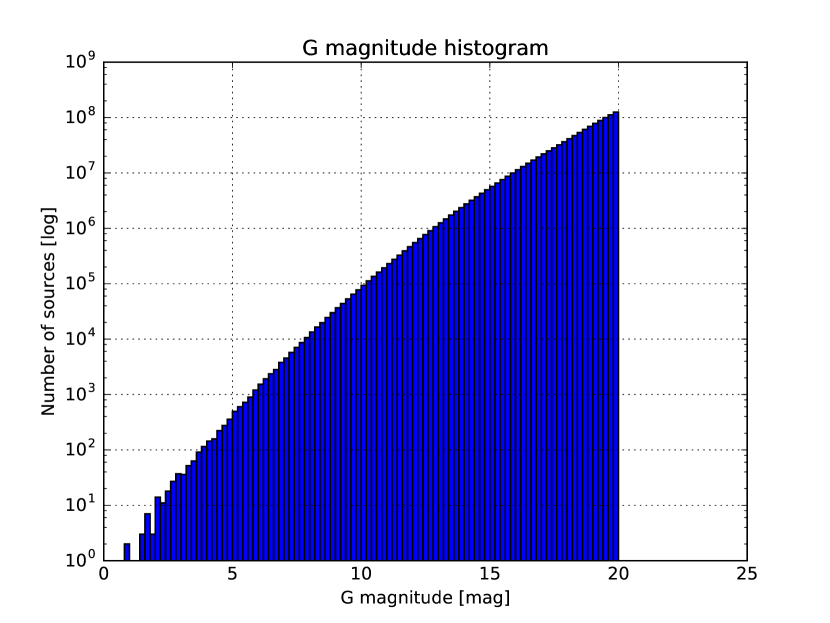
To compute the Gaia potential observables, standard uncertainties must be added to the simulation. Because astrometric quantities (positions, parallaxes, and proper motions) are related, a single formalism to derive its standard errors is needed. PyGaia implements a simple performance model depending on the colour term and the magnitude to estimate the end-of-mission errors for the parallax uncertainty:
| (26) |
with
| (27) |
(see the Gaia science performance web for more details). It also takes into account the variation of the uncertainties over the sky because of the scanning law, tabulated as a function of the ecliptic latitude666https://www.cosmos.esa.int/web/gaia/table-2-with-ascii .
However, these are end-of-mission uncertainties, so they have to be scaled by the fraction of mission time completed in order to get an estimation of them for Gaia DR2 . In the case of the parallax, only the factor , being the mission time (years) included in Gaia DR2 , need to be applied; this error model is further described in Arenou et al. (2017). In our case we have also updated the calibration floor to take into account the properties of the Gaia DR2 formal errors, as shown in Fig. 17. This calibration floor introduces a minimum formal error stemming from the fact that the calibrations used in the data processing (models and parameters) are at this stage still being refined. This floor affects mainly bright stars, while for faint stars the photon noise dominates. Fig. 17 shows the model used in the simulation for the Gaia DR2 parallax uncertainties as a function of the magnitude.
