Gaia Data Release 2: first stellar parameters from Apsis
The second Gaia data release (Gaia DR2) contains, beyond the astrometry, three-band photometry for 1.38 billion sources. One band is the G band, the other two were obtained by integrating the Gaia prism spectra (BP and RP). We have used these three broad photometric bands to infer stellar effective temperatures, , for all sources brighter than mag with in the range 3 000–10 000 K (some 161 million sources). Using in addition the parallaxes, we infer the line-of-sight extinction, , and the reddening, , for 88 million sources. Together with a bolometric correction we derive luminosity and radius for 77 million sources. These quantities as well as their estimated uncertainties are part of Gaia DR2. Here we describe the procedures by which these quantities were obtained, including the underlying assumptions, comparison with literature estimates, and the limitations of our results. Typical accuracies are of order 324 K (), 0.46 mag (), 0.23 mag (), 15% (luminosity), and 10% (radius). Being based on only a small number of observable quantities and limited training data, our results are necessarily subject to some extreme assumptions that can lead to strong systematics in some cases (not included in the aforementioned accuracy estimates). One aspect is the non-negativity contraint of our estimates, in particular extinction, which we discuss. Yet in several regions of parameter space our results show very good performance, for example for red clump stars and solar analogues. Large uncertainties render the extinctions less useful at the individual star level, but they show good performance for ensemble estimates. We identify regimes in which our parameters should and should not be used and we define a “clean” sample. Despite the limitations, this is the largest catalogue of uniformly-inferred stellar parameters to date. More precise and detailed astrophysical parameters based on the full BP/RP spectrophotometry are planned as part of the third Gaia data release.
Key Words.:
methods: data analysis – methods: statistical – stars: fundamental parameters – surveys: Gaia1 Introduction
The main objective of ESA’s Gaia satellite is to understand the structure, formation, and evolution of our Galaxy from a detailed study of its constituent stars. Gaia’s main technological advance is the accurate determination of parallaxes and proper motions for over one billion stars. Yet the resulting three-dimensional maps and velocity distributions which can be derived from these are of limited value if the physical properties of the stars remain unknown. For this reason Gaia is equipped with both a low-resolution prism spectrophotometer (BP/RP) operating over the entire optical range, and a high-resolution spectrograph (RVS) observing from 845–872 nm (the payload is described in Gaia Collaboration et al. 2016).
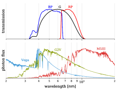
The second Gaia data release (Gaia DR2, Gaia Collaboration et al., 2018b) contains a total of 1.69 billion sources with positions and G-band photometry based on 22 months of mission observations. Of these, 1.33 billion sources also have parallaxes and proper motions (Lindegren et al., 2018). Unlike in the first release, Gaia DR2 also includes the integrated fluxes from the BP and RP spectrophotometers. These prism-based instruments produce low resolution optical spectrophotometry in the blue and red parts of the spectra which will be used to estimate astrophysical parameters for stars, quasars, and unresolved galaxies using the Apsis data processing pipeline (see Bailer-Jones et al. 2013). They are also used in the chromatic calibration of the astrometry. The processing and calibration of the full spectra is ongoing, and for this reason only their integrated fluxes, expressed as the two magnitudes and , are released as part of Gaia DR2 (see Fig. 1). The production and calibration of these data are described in Riello et al. (2018). 1.38 billion sources in Gaia DR2 have integrated photometry in all three bands, , , and (Evans et al., 2018), and 1.23 billion sources have both five-parameter astrometry and three-band photometry.
In this paper we describe how we use the Gaia three-band photometry and parallaxes, together with various training data sets, to estimate the effective temperature , line-of-sight extinction and reddening , luminosity , and radius , of up to 162 million stars brighter than =17 mag (some of these results are subsequently filtered out of the catalogue). We only process sources for which all three photometric bands are available. This therefore excludes the so-called bronze sources (Riello et al., 2018). Although photometry for fainter sources is available in Gaia DR2, we chose to limit our analysis to brighter sources on the grounds that, at this stage in the mission and processing, only these give sufficient photometric and parallax precision to obtain reliable astrophysical parameters. The choice of =17 mag was somewhat arbitrary, however.111The original selection was mag, but due to a later change in the zeropoint, our final selection is actually mag. The work described here was carried out under the auspices of the Gaia Data Processing and Analysis Consortium (DPAC) within Coordination Unit 8 (CU8) (see Gaia Collaboration et al. 2016 for an overview of the DPAC). We realise that more precise, and possibly more accurate, estimates of the stellar parameters could be made by cross-matching Gaia with other survey data, such as GALEX (Morrissey et al., 2007), PanSTARRS (Chambers et al., 2016), and WISE (Cutri et al., 2014). However, the remit of the Gaia-DPAC is to process the Gaia data. Further exploitation, by including data from other catalogues, for example, is left to the community at large. We nonetheless hope that the provision of these “Gaia-only” stellar parameters will assist the exploitation of Gaia DR2 and the validation of such extended analyses.
We continue this article in section 2 with an overview of our approach and its underlying assumptions. This is followed by a description of the algorithm – called Priam – used to infer , , and in section 3, and a description of the derivation of and – with the algorithm FLAME – in section 4. The results and the content of the catalogue are presented in section 5. More details on the catalogue itself (data fields etc.) can be found in the online documentation accompanying the data release. In section 6 we validate our results, in particular via comparison with other determinations in the literature. In section 7 we discuss the use of the data, focusing on some selections which can be used to identify certain types of stars, as well as the limitations of our results. This is mandatory reading for anyone using the catalogue. Priam and FLAME are part of a larger astrophysical parameter inference system in the Gaia data processing (Apsis). Most of the algorithms in Apsis have not been activated for Gaia DR2. (Priam itself is part of the GSP-Phot software package, which uses several algorithms to estimate stellar parameters.) We look ahead in section 8 to the improvements and extensions of our results which can be expected in Gaia DR3. We summarize our work in section 9. We draw attention to appendix B, where we define a “clean” subsample of our results.
In this article we will present both the estimates of a quantity and the estimates of its uncertainty, and we will also compare the estimated quantity with values in the literature. The term uncertainty refers to our computed estimate of how precise our estimated quantity is. This is colloquially (and misleadingly) called an “error bar”. We provide asymmetric uncertainties in the form of two percentiles from a distribution (upper and lower). We use the term error to refer to the difference between an estimated quantity and its literature estimate, whereby this difference could arise from a mistake in our estimate, in the literature value, or in both.
2 Approach and assumptions
2.1 Overview of procedure
We estimate stellar parameters source-by-source, using only the three Gaia photometric bands (for ) and additionally the parallax (for the other four parameters). We do not use any non-Gaia data on the individual sources, and we do not make use of any global Galactic information, such as an extinction map or kinematics.
The three broad photometric bands – one of which is near degenerate with the sum of the other two (see Fig. 1) – provide relatively little information for deriving the intrinsic properties of the observed Gaia targets. They are not sufficient to determine whether the target is really a star as opposed to a quasar or an unresolved galaxy, for example. According to our earlier simulations, this will ultimately be possible using the full BP/RP spectra (using the Discrete Source Classifier in Apsis). As we are only working with sources down to =17, it is reasonable to suppose that most of them are Galactic. Some will, inevitably, be physical binaries in which the secondary is bright enough to affect the observed signal. We nonetheless proceed as though all targets were single stars. Some binarity can be identified in the future using the composite spectrum (e.g. with the Multiple Star Classifier in Apsis) or the astrometry, both of which are planned for Gaia DR3.
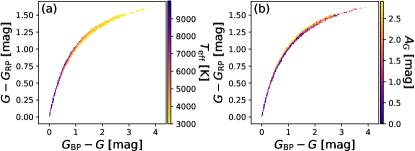
Unsurprisingly, is heavily degenerate with in the Gaia colours (see Fig. 2), so it seems near impossible that both quantities could be estimated from only colours. Our experiments confirm this. We work around this by estimating from the colours on the assumption that the star has (ideally) zero extinction. For this we use an empirically-trained machine learning algorithm (nowadays sometimes referred to as “data driven”). That is, the training data are observed Gaia photometry of targets which have had their estimated from other sources (generally spectroscopy). This training data set only includes stars which are believed to have low extinctions.
We separately estimate the interstellar absorption using the three bands together with the parallax, again using a machine learning algorithm. By using the magnitudes and the parallax, rather than the colours, the available signal is primarily the dimming of the sources due to absorption (as opposed to just the reddening). For this we train on synthetic stellar spectra, because there are too few stars with reliably estimated extinctions which could be used as an empirical training set. Note that the absorption we estimate is the extinction in the G-band, , which is not the same as the (monochromatic) extinction parameter, . The latter depends only on the amount of absorption in the interstellar medium, whereas the former depends also on the spectral energy distribution (SED) of the star (see section 2.2 of Bailer-Jones 2011).222We distinguish between the -band extinction (which depends on the intrinsic source SED) and the monochromatic extinction at a wavelength of nm (which is a parameter of the extinction law and does not depend on the intrinsic source SED). Thus even with fixed there is not a one-to-one relationship between and . For this reason we use a separate model to estimate the reddening , even though the available signal is still primarily the dimming due to absorption. By providing estimates of both absorption and reddening explicitly, it is possible to produce a de-reddened and de-extincted colour–magnitude diagram.
| band | zeropoint () [mag] |
|---|---|
The inputs for our processing are fluxes, , provided by the upstream processing (Riello et al., 2018). We convert these to magnitudes, , using
| (1) |
where is the zeropoint listed in Table 1. All of our results except depend on these zeropoints.
We estimate the absolute G-band magnitude via the usual equation
| (2) |
This is converted to a stellar luminosity using a bolometric correction (see section 4). The distance to the target is taken simply to be the inverse of the parallax. Although this generally gives a biased estimate of the distance (Bailer-Jones, 2015; Luri et al., 2018), the impact of this is mitigated by the fact that we only report luminosities when the fractional parallax uncertainty is less than 0.2. Thus, of the 161 million stars with estimates, only 77 million have luminosity estimates included in Gaia DR2.
Having inferred the luminosity and temperature, the stellar radius is then obtained by applying the Stefan–Boltzmann law
| (3) |
Because our individual extinction estimates are rather poor for most stars (discussed later), we chose not to use them in the derivation of luminosities, i.e. we set to zero in equation 2. Consequently, while our temperature, luminosity, and radius estimates are self-consistent (within the limits of the adopted assumptions), they are formally inconsistent with our extinction and reddening estimates.
The final step is to filter out the most unreliable results: these do not appear in the catalogue (see appendix A). We furthermore recommend that for , only the “clean” subsample of our results be used. This is defined and identified using the flags in appendix B. When using extinctions, users may further want to make a cut to only retain stars with lower fractional parallax uncertainties.
2.2 Data processing
The software for Apsis is produced by teams in Heidelberg, Germany (Priam) and Nice, France (FLAME). The actual execution of the Apsis software on the Gaia data is done by the DPCC (Data Processing Centre CNES) in Toulouse, which also integrates the software. The processing comprises several operations, including the input and output of data and generation of logs and execution reports. The entire process is managed by a top-level software system called SAGA. Apsis is run in parallel on a multi-core Hadoop cluster system, with data stored in a distributed file system. The validation results are published on a web server (GaiaWeb) for download by the scientific software providers. The final Apsis processing for Gaia DR2 took place in October 2017. The complete set of sources (1.69 billion with photometry) covering all Gaia magnitudes was ingested into the system. From this the 164 million sources brighter than =17 mag were identified and processed. This was done on 1000 cores (with 6 GB RAM per core), and ran in about 5000 hours of CPU time (around five hours wall clock time). The full Apsis system, which involves much more CPU-intensive processes, higher-dimensional input data (spectra), and of order one billion sources, will require significantly more resources and time.
3 Priam
3.1 General comments
Once the dispersed BP/RP spectrophotometry are available, the GSP-Phot software will estimate a number of different stellar parameters for a range of stellar types (see Liu et al., 2012; Bailer-Jones et al., 2013). For Gaia DR2 we use only the Priam module within GSP-Phot to infer parameters using integrated photometry and parallax. All sources are processed even if they have corrupt photometry (see Fig. 4) or if the parallax is missing or non-positive. Some results are flagged and others filtered from the catalogue (see appendix A).
Priam employs extremely randomised trees (Geurts et al., 2006, hereafter ExtraTrees), a machine learning algorithm with a univariate output. We use an ensemble of 201 trees and take the median of their outputs as our parameter estimate.333Further ExtraTrees regression parameters are random trials per split and minimal stars per leaf node. We use the 16th and 84th percentiles of the ExtraTrees ensemble as two uncertainty estimates; together they form a central 68% confidence interval. Note that this is, in general, asymmetric with respect to the parameter estimate. 201 trees is not very many from which to accurately compute such intervals – a limit imposed by available computer memory – but our validation shows them to be reasonable. ExtraTrees are incapable of extrapolation: they cannot produce estimates or confidence intervals outside the range of the target variable (e.g. ) in the training data. We experimented with other machine learning algorithms, such as support vector machine (SVM) regression (e.g. Deng et al., 2012) and Gaussian processes (e.g. Bishop, 2006), but we found ExtraTrees to be much faster (when training is also considered), avoid the high sensitivity of SVM tuning, and yet still provide results which are as good as any other method tried.
3.2 Effective temperatures
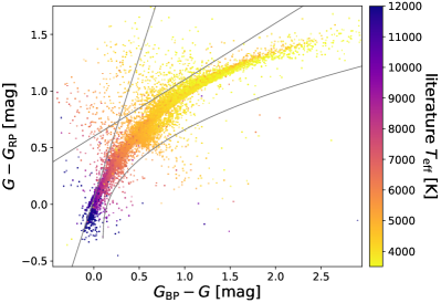
Given the observed photometry , , and , we use the distance-independent colours and as the inputs to ExtraTrees to estimate the stellar effective temperature . These two colours exhibit a monotonic trend with (Fig. 3). It is possible to form a third colour, , but this is not independent, plus it is noisier since it does not contain the higher signal-to-noise ratio -band. We do not propagate the flux uncertainties through ExtraTrees. Furthermore, the integrated photometry is calibrated with two different procedures, producing so-called “gold-standard” and “silver-standard” photometry (Riello et al., 2018). As shown in Fig. 3, gold and silver photometry provide the same colour-temperature relations, thus validating the consistency of the two calibration procedures of Riello et al. (2018).

Since the in-flight instrument differs from its nominal pre-launch prescription (Jordi et al., 2010; de Bruijne, 2012), in particular regarding the passbands (see Fig. 1), we chose not to train ExtraTrees on synthetic photometry for . Even though the differences between nominal and real passbands are probably only of the order of 0.1 mag or less in the zeropoint magnitudes (and thus even less in colours), we obtained poor estimates, with differences of around 800 K compared to literature values when using synthetic colours from the nominal passbands. We instead train ExtraTrees on Gaia sources with observed photometry and labels taken from various catalogues in the literature. These catalogues use a range of data and methods to estimate : APOGEE (Alam et al., 2015) uses mid-resolution, near-infrared spectroscopy; the Kepler Input Catalogue444https://archive.stsci.edu/pub/kepler/catalogs/ file kic_ct_join_12142009.txt.gz (Huber et al., 2014) uses photometry; LAMOST (Luo et al., 2015) uses low-resolution optical spectroscopy; RAVE (Kordopatis et al., 2013) uses mid-resolution spectroscopy in a narrow window around the Caii triplet. The RVS auxiliary catalogue (Soubiran et al., 2014; Sartoretti et al., 2018), which we also use, is itself is a compilation of smaller catalogues, each again using different methods and different data. By combining all these different catalogues we are deliberately “averaging” over the systematic differences in their estimates. The validation results presented in sections 5 and 6 will show that this is not the limiting factor in our performance, however. This data set only includes stars which have low extinctions (although not as low as we would have liked). 95% of the literature estimates for these stars are below 0.705 mag for and 0.307 mag for . (50% are below 0.335 mag and 0.13 mag respectively.) These limits exclude the APOGEE part of the training set, for which no estimates of or are provided. While APOGEE giants in particular can reach very high extinctions, they are too few to enable ExtraTrees to learn to disentangle the effects of temperature and extinction in the training process. The training set is mostly near-solar metallicity stars: 95% of the stars have and 99% have .
We compute our magnitudes from the fluxes provided by the upstream processing using equation 1. The values of the zeropoints used here are unimportant, however, because the same zeropoints are used for both training and application data.
| number | mean | |
|---|---|---|
| catalogue | of stars | uncertainty [K] |
| APOGEE | 5 978 | 92 |
| Kepler Input Catalogue | 14 104 | 141 |
| LAMOST | 5 540 | 55 |
| RAVE | 2 427 | 61 |
| RVS Auxiliary Catalogue | 4 553 | 122 |
| combined | 32 602 | 102 |
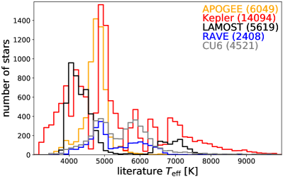
We only retain stars for training if the catalogue specifies a uncertainty of less than 200K, and if the catalogue provides estimates of and . The resulting set of 65 000 stars, which we refer to as the reference sample, is shown in Figs. 3 and 4. We split this sample into near-equal-sized training and test sets. To make this split reproducible, we use the digit sum of the Gaia source ID (a long integer which is always even): sources with even digit sums are used for training, those with odd for testing. The temperature distribution of the training set is shown in Fig. 5 (that for the test set is virtually identical). The distribution is very inhomogeneous. The impact of this on the results is discussed in section 5.2. Our supervised learning approach implicitly assumes that the adopted training distribution is representative of the actual temperature distribution all over the sky, which is certainly not the case (APOGEE and LAMOST probe quite different stellar populations, for example). However, such an assumption – that the adopted models are representative of the test data – can hardly be avoided. We minimise its impact by combining many different literature catalogues covering as much of the expected parameter space as possible.
Table 2 lists the number of stars (in the training set) from each catalogue, along with their typical uncertainty estimates as provided by that catalogue (which we will use in section 5.1 to infer the intrinsic temperature error of Priam).555The subsets in Table 2 are so small that there are no overlaps between the different catalogues. Also note that the uncertainty estimates provided in the literature are sometimes clearly too small, e.g. for LAMOST. Mixing catalogues which have had estimated by different methods is likely to increase the scatter (variance) in our results, but it is a property of ExtraTrees that this averaging should correspondingly reduce the bias in our results. Such a mixture is necessary, because no single catalogue covers all physical parameter space with a sufficiently large number of stars for adequate training. Even with this mix of catalogues we had to restrict the temperature range to 3000K10 000K, since there are too few literature estimates outside of this range to enable us to get good results. For instance, there are only a few hundred OB stars with published estimates (Ramírez-Agudelo et al., 2017; Simón-Díaz et al., 2017). We tried to extend the upper temperature limit by training on white dwarfs with estimates from Kleinman et al. (2013), but as Fig. 3 reveals, the colour-temperature relations of white dwarfs (black points) differ significantly from those of OB stars (orange points with K). Since ExtraTrees cannot extrapolate, this implies that stars with true K or K are “thrown back” into the interval 3000K–10 000K (see section 6.3). This may generate peculiar patterns when, for example, plotting a Hertzsprung–Russell diagram (see section 5.2).
The colour–colour diagram shown in Fig. 4 exhibits substantially larger scatter than expected from the PARSEC models shown in Fig. 2, even inside the selected good-quality region. This is not due to the measurement errors on fluxes, as the formal uncertainties in Fig. 4 are smaller than dot size for 99% of the stars plotted. Instead, this larger scatter reflects a genuine astrophysical diversity that is not accounted for in the models (for example due to metallicity variations, whereas Fig. 2 is restricted to ).
3.3 Line-of-sight extinctions
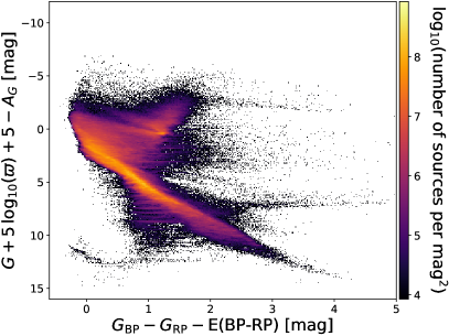
For the first time, Gaia DR2 provides a colour–magnitude diagram for hundreds of millions of stars with good parallaxes. We complement this with estimates of the -band extinction and the reddening such that a dust-corrected colour-magnitude diagram can be produced.
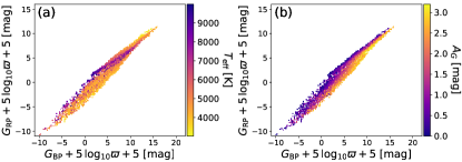
As expected, we were unable to estimate the line-of-sight extinction from just the colours, since the colour is strongly influenced by (Fig. 2a vs. b). We therefore use the parallax to estimate the distance and then use equation (2) to compute for all three bands (which isn’t directly measured, but for convenience we refer to it from now on as an observable). We then use the three observables , , as features for training ExtraTrees. As shown in Fig. 6b, there is a clear extinction trend in this observable space, whereas the dependence on (Fig. 6a) is much less pronounced than in colour-colour space (Fig. 2a). Yet, extinction and temperature are still very degenerate in some parts of the parameter space, and also there is no unique mapping of to extinction thus leading to further degeneracies (see section 6.5). Dependence on the parallax here restricts us to stars with precise parallaxes, but we want to estimate and in order to correct the colour-magnitude diagram (CMD), which itself is already limited by parallax precision. We do not propagate the flux and parallax uncertainties through ExtraTrees.666We found that propagating the flux and parallax uncertainties through the ExtraTrees has no noteworthy impact on our results, i.e. our extinction and reddening estimates are not limited by the expected precision of the input data.
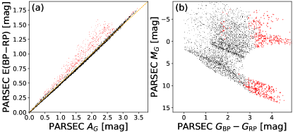
In order to estimate extinction we cannot train our models on literature values, for two reasons. First, there are very few reliable literature estimate of the extinction. Second, published estimates are of and/or E() rather than and . We therefore use the PARSEC 1.2S models777http://stev.oapd.inaf.it/cgi-bin/cmd to obtain integrated photometry from the synthetic Atlas 9 spectral libraries (Castelli & Kurucz, 2003) and the nominal instrument passbands (Fig. 1). These models use the extinction law from Cardelli et al. (1989) and O’Donnell (1994) with a fixed relative extinction parameter, =3.1. We constructed a model grid that spans –4 mag, a temperature range of 2 500–20 000 K, a range of 1–6.5 dex, and a fixed solar metallicity (, ). We chose solar metallicity for our models since we could not cover all metallicities and because we expect most stars in our sample to have . The extinctions , , and the reddening are then computed for each star by subtracting from the extincted magnitudes the unextincted magnitudes (which are obtained for mag). We used the sampling of the PARSEC evolutionary models as is, without further rebalancing or interpolation. Since this sampling is optimised to catch the pace of stellar evolution with time, the underlying distribution of temperatures, masses, ages, and extinctions is not representative of the Gaia sample. Therefore, as for , this will have an impact on our extinction estimates. However, while the Gaia colours are highly sensitive to , the photometry alone hardly allows us to constrain extinction and reddening, such that we expect that artefacts from this mismatch of the distributions in training data and real data will be washed out by random noise.
We use two separate ExtraTrees models, one for and one for . The input observables are , , and in both cases. That is, we do not infer from colour measurements. On account of the extinction law, and are strongly correlated to the relation over most of our adopted temperature range, as can be seen in Fig. 7.888Using different stellar atmosphere models with different underlying synthetic SEDs, Jordi et al. (2010) found a slightly different relation between and . The finite scatter is due to the different spectral energy distributions of the stars: the largest deviations occur for very red sources. Note that because ExtraTrees cannot extrapolate beyond the training data range, we avoid negative estimates of and . This non-negativity means the likelihood cannot be Gaussian, and as discussed in appendix E, a truncated Gaussian is more appropriate.
Evidently, the mismatch between synthetic and real Gaia photometry, i.e. differences between passbands used in the training and the true passbands (and zeropoints), will have a detrimental impact on our extinction estimates, possibly leading to systematic errors. Nonetheless, this mismatch is only 0.1mag in the zeropoints (Evans et al., 2018) and as shown in Gaia Collaboration et al. (2018a), the synthetic photometry (using inflight passbands) of isochrone models actually agrees quite well with the Gaia data. Indeed, as will be shown in sections 5.2 and 6.6, this mismatch appears not to lead to obvious systematic errors.999The situation for would be different, where using synthetic colours results in large errors.
Although we cannot estimate temperatures from these models with our data, the adopted range of 2500–20 000 K for the PARSEC models allows us to obtain reliable extinction and reddening estimates for intrinsically very blue sources such as OB stars, even though the method described in section 3.2 cannot provide good estimates for them.
4 FLAME
The Final Luminosity, Age, and Mass Estimator (FLAME) module aims to infer fundamental parameters of stars. In Gaia DR2 we only activate the components for inferring luminosity and radius. Mass and age will follow in the next data release, once GSP-Phot is able to estimate and from the BP/RP spectra and the precision in and improves. We calculate luminosity with
| (4) |
where is in units of (Table 3), is the absolute magnitude of the star in the G-band, is a temperature dependent bolometric correction (defined below), and mag is the solar bolometric magnitude as defined in IAU Resolution 2015 B2101010https://www.iau.org/static/resolutions/IAU2015_English.pdf. The absolute magnitude is computed from the G-band flux and parallax using equations 1 and 2. As the estimates of extinction provided by Priam were shown not to be sufficiently accurate on a star-to-star basis for many of our brighter validation targets, we set to zero when computing . The radius is then calculated from equation 3 using this luminosity and from Priam. These derivations are somewhat trivial; at this stage FLAME simply provides easy access for the community to these fundamental parameters.
Should a user want to estimate luminosity or radius assuming a non-zero extinction and/or a change in the bolometric correction of , one can use the following expressions
| (5) |
| (6) |
| quantity | unit | value |
|---|---|---|
| m | ||
| K | ||
| W | ||
| mag | ||
| mag | ||
| mag | ||
| mag | ||
| mag |
4.1 Bolometric Correction
We obtained the bolometric correction on a grid as a function of , , , and , derived from the MARCS synthetic stellar spectra (Gustafsson et al., 2008). The synthetic spectra cover a range from 2500K to 8000K, from 0.5 to 5.5 dex, from 5.0 to +1.0 dex, and from +0.0 to +0.4 dex. Magnitudes are computed from the grid spectra using the G filter (Fig. 1). These models assume local thermodynamic equilibrium (LTE), with plane-parallel geometry for dwarfs and spherical symmetry for giants. We extended the range using the from Jordi et al. (2010), but with an offset added to achieve continuity with the MARCS models at 8000 K. However, following the validation of our results (discussed later), we choose to filter out FLAME results for stars with outside the range 3300 – 8000 K (see appendix A).
For the present work we had to address two issues. First, is a function of four stellar parameters, but it was necessary to project this to be a function of just , since for Gaia DR2 we do not yet have estimates of the other three stellar parameters. Second, the bolometric correction needs a reference point to set the absolute scale, as this is not defined by the models. We will refer to this as the offset of the bolometric correction, and it has been defined here so that the solar bolometric correction is +0.06 mag. Further details are provided in appendix D.
To provide a 1-D bolometric correction, we set =0 and select the corresponding111111Choosing or including only changed the in the third decimal place, well below its final uncertainty. Fixing to a single value (e.g. zero) had just as little impact relative to the uncertainty. to . As there is still a dependence on , we adopt for each bin the mean value of the bolometric correction. We also compute the standard deviation as a measure of the uncertainty due to the dispersion in . We then fit a polynomial to these values to define the function
| (7) |
The values of the fitted coefficients are given in Table 4. The fit is actually done with the offset parameter fixed to mag, the reference bolometric value of the Sun (see appendix D). We furthermore make two independent fits, one for the in the range 4000–8000 K and another for the range 3300–4000 K.
| 4000 – 8000 K | ||
| 6.000e | 2.634e | |
| 6.731e | 2.438e | |
| 6.647e | 1.129e | |
| 2.859e | 6.722e | |
| 7.197e | 1.635e | |
| 3300 – 4000 K | ||
| 1.749e | 2.487e | |
| 1.977e | 1.876e | |
| 3.737e | 2.128e | |
| 8.966e | 3.807e | |
| 4.183e | 6.570e | |
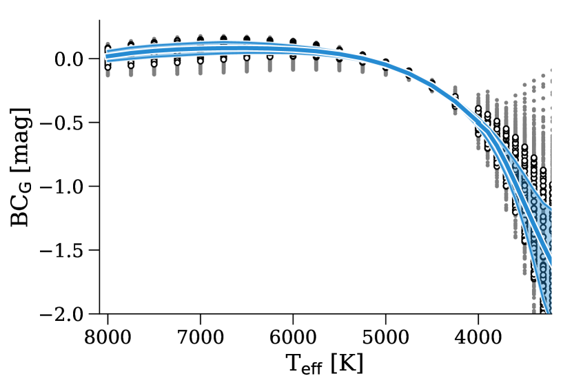
Fig. 8 shows as a function of . The largest uncertainty is found for K where the spread in the values can reach up to 0.3 mag, due to not distinguishing between giants and dwarfs121212We could have estimated a mass from luminosities and colours in order to estimate , and subsequently iterated to derive new luminosities and radii. However, given the uncertainties in our stellar parameters, we decided against doing this.. We estimated the uncertainty in the bolometric correction by modelling the scatter due to as a function of , using the same polynomial model as in equation 7. The coefficients for this model are also listed in Table 4.
4.2 Uncertainty estimates on luminosity and radius
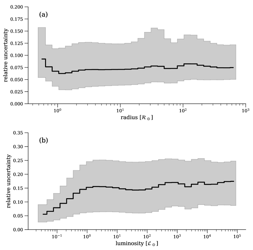
The upper and lower uncertainty levels for are defined symmetrically as , where has been calculated using a standard (first order) propagation of the uncertainties in the G-band magnitude and parallax131313A revision of the parallax uncertainties between processing and the data release means that our fractional luminosity uncertainties are incorrect by factors varying between 0.6 and 2 (for 90% of the stars), with some dependence on magnitude (see appendix A of Lindegren et al. (2018), in particular the upper panel of Figure A.2). Although there was no opportunity to rederive the luminosity uncertainties, these revised parallax uncertainties (i.e. those in Gaia DR2) were used when filtering the FLAME results according to the criterion in appendix A.. Note, however, that we do not include the additional uncertainty arising from the temperature which would propagate through the bolometric correction (equation 4). For , the upper and lower uncertainty levels correspond to the radius computed using the upper and lower uncertainty levels for . As these levels are 16th and 84th percentiles of a distribution, and percentiles are conserved under monotonic transformations of distributions, the resulting radius uncertainty levels are also the 16th and 84th percentiles. This transformation neglects the luminosity uncertainty, but in most cases the uncertainty dominates for the stars in the published catalogue (i.e. filtered results; see Appendix A). The distribution of the uncertainties in and for different parameter ranges are shown as histograms in Figs. 9. The radius uncertainty defined here is half the difference between the upper and lower uncertainty levels. It can be seen that the median uncertainties in , which considers just the uncertainties in and , is around 15%. For radius it’s typically less than 10%. While our uncertainty estimates are not particularly precise, they provide the user with some estimate of the quality of the parameter.
5 Results and catalogue content
We now present the Apsis results in Gaia DR2 by looking at the performance on various test data sets. We refer to summaries of the differences between our results and their literature values as “errors”, as by design our algorithms are trained to achieve minimum differences for the test data. This does not mean that the literature estimates are “true” in any absolute sense. We ignore here the inevitable inconsistencies in the literature values, since we do not expect our estimates to be good enough to be substantially limited by these.
5.1 Results for
We use the test data set (as defined in section 3.2) to examine the quality of our estimates. We limit our analyses to those 98% of sources which have “clean” Priam flags for (defined in appendix B). Our estimated values range from 3229 K to 9803 K on this test set. The smallest lower uncertainty level is 3098 K and the highest upper uncertainty level is 9985 K. As the uncertainties are percentiles of the distribution of ExtraTrees outputs, and this algorithm cannot extrapolate, these are constrained to the range of our training data (which is 3030 K to 9990 K).
| reference catalogue | bias [K] | RMS error [K] |
|---|---|---|
| APOGEE | 105 | 383 |
| Kepler Input Catalogue | 6 | 232 |
| LAMOST | 9 | 381 |
| RAVE | 21 | 216 |
| RVS Auxiliary Catalogue | 50 | 425 |
| GALAH | 18 | 233 |
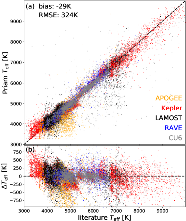
Fig. 10 compares our estimates with the literature estimates for our test data set. The root-mean-squared (RMS) test error is 324 K, which includes a bias (defined as the mean residual) of K. For comparison, the RMS error on the training set is 217 K, with a bias of K (better than the test set, as expected). We emphasise that the RMS test error of 324 K is an average value over the different catalogues, which could have different physical scales. Moreover, since our test sample, just like our training sample, is not representative for the general stellar population in Gaia DR2, the 324 K uncertainty estimate is likely to be an underestimate. Nevertheless, given this RMS test error of 324 K, we can subtract (in quadrature) the 102 K literature uncertainty (Table 2) to obtain an internal test error estimate of 309 K for Priam.
Table 5 shows that the errors vary considerably for the different reference catalogues. Consequently, the temperature errors for a stellar population with a restricted range of could differ from our global estimates (see sections 6.3 and 6.4). This is illustrated in panels (a) and (b) of Fig. 11. If the estimated temperature is below about 4000 K, we can expect errors of up to 550 K. Likewise, if the estimated temperature is above 8000 K, the absolute error increases while the relative error is consistently below 10% for K. The dependence of test error on literature temperatures (Fig. 11c) shows the same behaviour. Note that the errors are dominated by outliers, since when we replace the mean by the median, the errors are much lower (solid vs. dashed lines in Fig. 11).
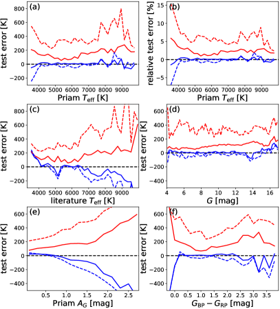
As we can see from Fig. 11d, the temperature error increases only very slightly with magnitude, which is best seen in the medians since outliers can wash out this trend in the means. Fig. 11e shows that the temperature error is weakly correlated with the estimated extinction, but now more dominant in the mean than the median. This is to be expected since our training data are mostly stars with low extinctions. Stars with high extinctions are under-represented, and due to the extinction–temperature degeneracy they are assigned systematically lower estimates. This is particularly apparent when we plot the temperature residuals in the Galactic coordinates (Fig. 12): stars in the Galactic plane, where extinctions are higher, have systematically negative residuals. Finally, Fig. 11f shows that the temperature error also depends on the colour of the star. Very blue and very red stars were comparatively rare in the training data. For the bluest stars, we see that we systematically underestimate . This is a direct consequence of the upper limit of 10 000 K in the training sample (but not in the Galaxy) and the inability of ExtraTrees to extrapolate.
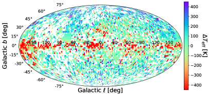
Fig. 12 also suggests a slight tendency to systematically overestimate at high Galactic latitudes. Halo stars typically have subsolar metallicity, hence tend to be bluer for a given than solar metallicity stars. This may lead Priam, which is trained mostly on solar-metallicity stars, to overestimate (see Sect. 6.1). Alternatively, although the extinction in our empirical training sample is generally low, it is not zero, such that for high latitude stars with almost zero extinction, Priam would overestimate . Most likely, both effects are at work, with the latter presumably dominating.
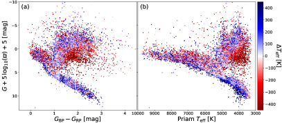
The differences between our temperature estimates and the literature values are shown in a CMD in Fig. 13a. Priam predicts lower in those parts of the CMD where we suspect the extinction may be high (e.g. the lower part of the giant branch). Conversely, the overestimation of in the lower part of the main sequence may be due nearby faint stars having lower extinctions than the low but non-zero extinction in our empirical training sample. These systematics with extinction agree with Fig. 11e. This will be discussed further in the next section.
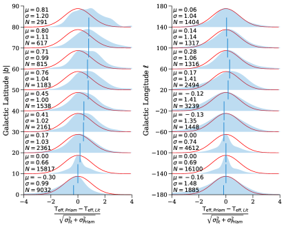
In order to assess our uncertainty estimates, we again use the test data. Ideally, the distribution of our uncertainty estimates should coincide with the distribution of the errors. We find that for 23% of test stars, their literature values are below our lower uncertainty levels (which are 16th percentiles), whereas for 22% of test stars the literature values are above our upper uncertainty levels (84th percentiles). One interpretation of this is that our uncertainty intervals are too narrow, i.e. that the supposed 68% central confidence interval (84th minus 16th) is in fact more like a 55% confidence interval. However, the literature estimates have finite errors, perhaps of order 100–200 K, and these will increase the width of the residual distribution (compared to computing residuals using perfect estimates). We investigate this more closely by plotting the distribution of residuals normalised by the combined (Priam and literature) uncertainty estimates. This is shown in Fig. 14 for all our test data and different directions in the Galaxy. If the combined uncertainties were Gaussian measures of the residuals, then the histograms should be Gaussian with zero mean and unit standard deviation (the red curves). This is generally the case, and suggests that, although we do not propagate the flux uncertainties, the Priam uncertainty estimates may indeed provide 68% confidence intervals and that the 55% obtained above arose only from neglecting literature uncertainties. The left column in Fig. 14 shows a systematic trend in the residuals (mean of the histogram) as a function of Galactic latitude, which is also evident from Fig. 12. This most likely reflects a systematic overestimation of for zero-extinction stars at high latitudes. Also note that the panels for and exhibit narrow peaks. These two panels are dominated by the Kepler field, which makes up 43% of the training sample (see Table 2). The fact that these two peaks are sharper than the unit Gaussian suggests overfitting of stars from the Kepler sample.141414Propagating the flux errors through the ExtraTrees gives slightly lower test errors (supporting the idea that we may overfit the Kepler sample) and brings the normalised residuals closer to a unit Gaussian. Concerning the asymmetry of the conference intervals, we find that for 57% of sources, upper minus median and median minus lower differ by less than a factor of two, while for 2.5% of sources these two bands can differ by more than a factor of ten.
5.2 Results for and
We look now at our estimates of line-of-sight extinction and reddening . Where appropriate we will select on parallax uncertainty. As will be discussed in section 6.5, some of our estimates of and suffered from strong degeneracies. These (about one third of the initial set of estimates) were filtered out of the final catalogue.
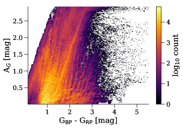
As explained in section 3.3, we are unable to estimate the line-of-sight extinction from just the colours. Fig. 15 demonstrates that neither nor has a one-to-one relation with the colour. (Plots against the other two colours are shown in the online Gaia DR2 documentation.) This complex distribution is the combined result of having both very broad filters and a wide range of stellar types. It may be possible to find an approximative colour–extinction relation only if one can a priori restrict the sample to a narrow part of the HRD, such as giant stars.
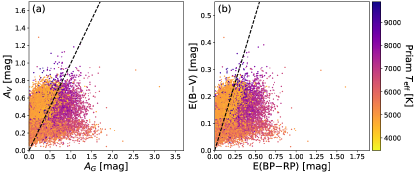
In addition, using only three optical bands (and parallax), we do not expect very accurate extinction estimates. A direct comparison to the literature is complicated by the fact that the literature does not estimate or but rather , , or . We compare them nonetheless on a star-by-star basis in Table 6, and Fig. 16 shows the results for stars for the Kepler Input Catalog. The largest RMS difference for these samples is 0.34 mag between and and 0.24 mag between and . This appears to be dominated primarily by systematically larger values of and . The differences between nominal and real passbands are only of order 0.1 mag in the zeropoints (Evans et al., 2018) and thus are unlikely to explain this. Instead, these large values arise from the degeneracies in the extinction estimation (see section 6.5) and the non-trivial transformation between and and between and . To mitigate this problem we validate using red clump stars in section 6.6. For now, we conclude from Table 6 that the scatter in may be as high as 0.34 mag and the scatter in as high as 0.24 mag. Given such a large scatter, we can only verify the extinction estimates at an ensemble level. Let us also emphasise that since ExtraTrees cannot produce negative results for or , the large random scatter may give rise to an apparent systematic error151515We show in appendix E that an apparent bias can arise if one uses the mean as an estimator when the likelihood is skewed. that can also be seen in Fig. 16. We also find an approximate relation (Fig. 17). This is essentially by construction, as we use the same PARSEC models for the determination of both quantities (see Fig. 7).
| Kepler Input Catalog | RMS | 0.34mag | 0.18mag |
|---|---|---|---|
| (15 143) | mean | 0.00mag | 0.07mag |
| Lallement et al. (2014) | RMS | – | 0.24mag |
| (1431 stars) | mean | – | 0.16mag |
| Rodrigues et al. (2014) | RMS | 0.21mag | – |
| (1315 stars) | mean | 0.08mag | – |
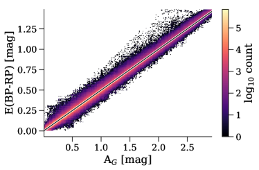
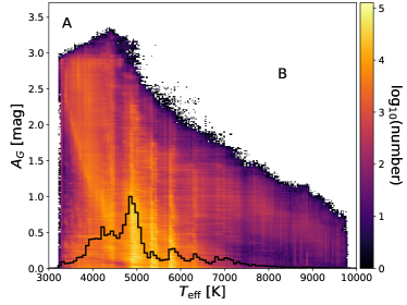
Fig. 18 shows the distribution of vs. for all stars with clean Priam flags. Since ExtraTrees cannot extrapolate from the training data range of 3000K–10 000K, the results are restricted to this range. We see unoccupied regions on this plot, labelled “A” and “B”. The empty region A is due to the apparent magnitude limit of , which removes stars with lower already at lower , since they are fainter. This is expected. However, the second empty region labelled B in Fig. 18 is more interesting. There are seemingly no hot stars with high extinctions. This void is an artefact and is due to our ExtraTrees training sample (for extinctions) comprising only low-extinction stars. Therefore, if hot stars in the overall sample are reddened by dust, they have no counterparts in the training sample and are thus assigned systematically lower temperatures which, given the training sample, is the only way that ExtraTrees can match their reddish colours. We also note the vertical stripes in Fig. 18, which are a consequence of the inhomogeneous temperature distribution in our training sample (see Fig. 5). Unfortunately, a desirable rebalancing of our training sample fell victim to the tight processing schedule for Gaia DR2. However, these results are not our final data products and revised training sets will be used for Gaia DR3 (section 8).
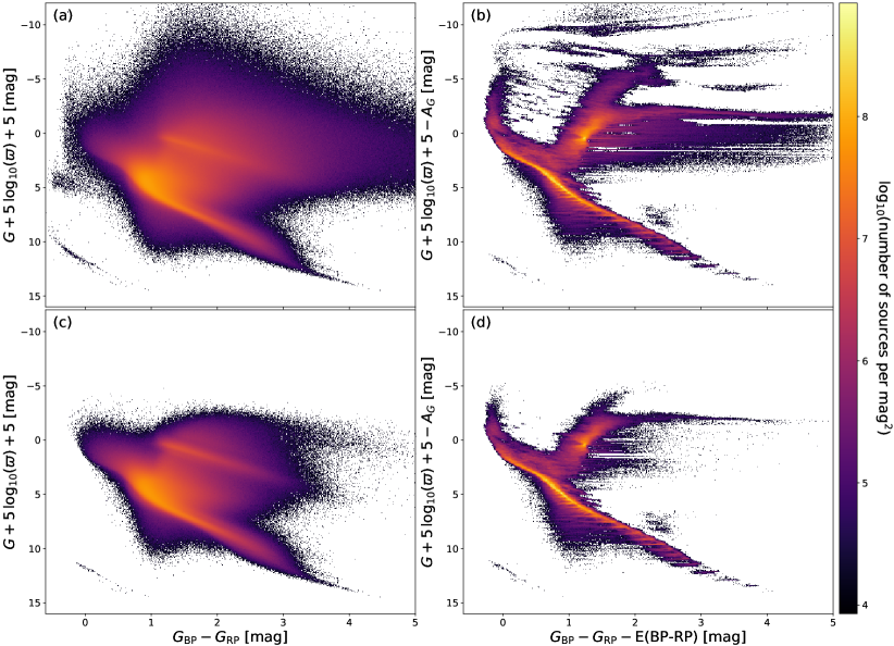
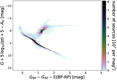
Although our extinction estimates are inaccurate on a star-by-star level, our main goal in estimating and is to enable a dust correction of the observed CMD. To this end, it is sufficient if our extinction estimates are mostly unbiased such that they are applicable at the ensemble level. This is often the case, as is shown in Fig. 19. The observed CMD in Fig. 19a exhibits a very diffuse source distribution. In particular, the giant branch is completely washed out, while the red clump is visible as a thin line above the main sequence, which is the result of dust extinction and reddening. If we use our estimates of and in order to correct the observed CMD, then we achieve Fig. 19b. This dust-corrected CMD is much less diffuse. In particular, the red clump is now an actual clump, the main sequence is more compact, and we can identify the giant branch. The horizontal stripes along the main sequence in Fig. 19b are artefacts that originate from the sampling of PARSEC evolutionary tracks which we took directly without further interpolation or smoothing. There are also horizontal streaks above the red giant branch, which are sources with poor parallaxes leading to a clustering in our results. Furthermore, there is a small group of 8587 sources (0.01% of all sources that have extinction estimates) just above the main sequence, which either are outliers that we failed to remove (see section 6.5) or which may be genuine binaries. If we additionally require the relative parallax uncertainty to be less than 20% (Bailer-Jones, 2015), then the observed CMD becomes Fig. 19c, which is much cleaner than Fig. 19a. The dust-corrected CMD corresponding to this – Fig. 19d – is likewise more distinct. In particular, the horizontal streaks above the giant branch are removed by cutting in relative parallax uncertainty. Nevertheless, Fig. 19 panels b and d also exhibit clear artefacts, some of which are due to bad parallaxes, although most are introduced by our methods and the training data. As all our models are only for single stars, binaries will receive systematically wrong extinction estimates. As most binaries reside above the main sequence, Priam will typically misinterpret them as highly reddened single stars from the upper part of the main sequence. Finally, we note that the logarithmic scale in Fig. 19 overemphasises the low-density regions, intentionally drawing the reader’s attention to the various artefacts. Nevertheless, our results produce a very thin main sequence, as is obvious from Fig. 20 which is exactly identical to Fig. 19b apart from a linear density scale.
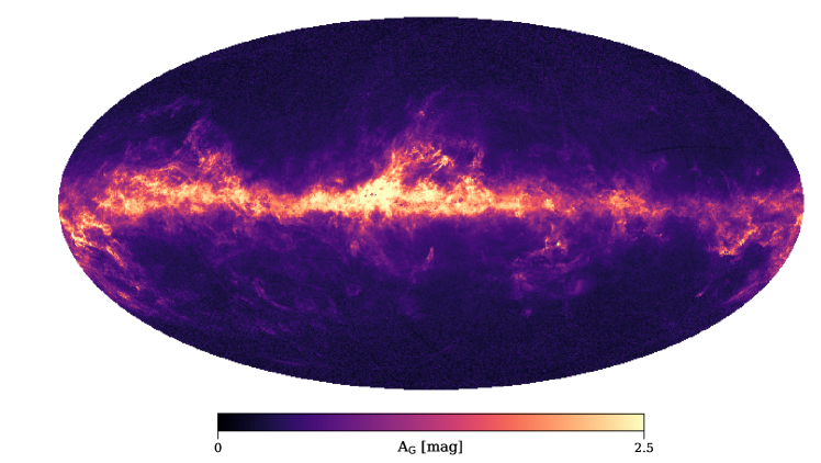
The statistical validity of our estimates is further attested to by Fig. 21. Recall that we do not use any sky position during our inference: each star estimate remains independent of any other.161616On account of this independence, plus the finite variance (guaranteed by the inability of ExtraTrees to extrapolate beyond the training range), the Central Limit Theorem applies to any average of our extinction or reddening estimates. This plot shows features quite distinct from just plotting the Gaia colour, as should be obvious from their lack of correlation (shown in Fig. 15). Plotting our extinction estimates on the sky not only highlights the Milky Way disk, but also numerous detailed substructures. Apart from the Small and Large Magellanic Clouds, we also recover a wealth of structure across a wide range of scales, from thin filaments to large cloud complexes. The Perseus, Taurus, and Auriga cloud complexes dominate the anticentral region (far left and right sides of the map, respectively), while the Orion molecular cloud complex () and the California nebula () show exquisite substructures, as does Ophiuchus just above the Galactic Center. More will be shown in section 6.7.
5.3 Results for
In this and the next subsection we describe the contents and the quality of the catalogue entries for and . We remind readers that upon validation of FLAME astrophysical parameters, several filters were put in place to remove individual entries, e.g. stars with 0.5 have no published radii or luminosities: see Appendix A for details. Only 48% of the entries with also have and (77 million stars). Unless otherwise specified, we present the results for the published catalogue.
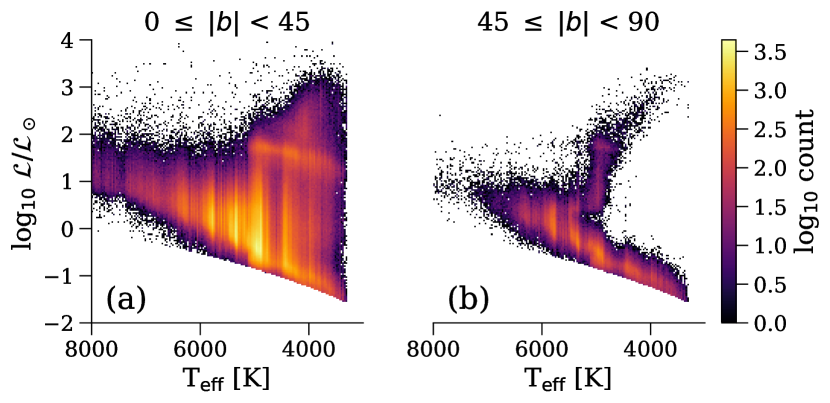
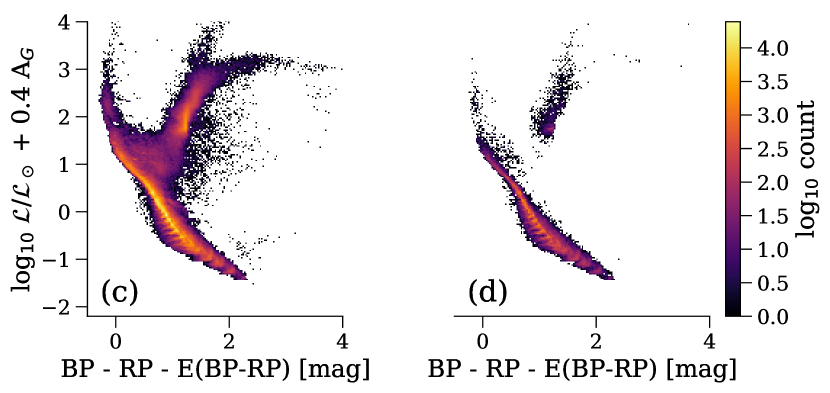
The quality and distribution of the luminosities in the catalogue can be best examined by constructing Hertzsprung–Russell Diagrams (HRD). The HRD using FLAME and Priam is shown in the top panels of Figure 22 separated by galactic latitude ( and ). For stars at lower galactic latitudes, our neglect of extinction in the luminosity estimation can lead to misinterpretations for individual stars or populations of stars. This can be seen in panel (a) where in particular the red giant branch is extended towards lower , and their luminosities appear lower (see also section 5.1). The vertical stripes at distinct values is a result of the inhomogeneous temperature distribution in the training sample (discussed in section 5.2, see Fig 5). The clean diagonal cut on the lower end is a direct result of our filtering out of sources with ¡ 0.5 . Replacing by de-reddened color in the abscissa, and including as given in equation 5, we see (in panel c) that the HRD tightens up nicely with a clear structure defining the main expected components. These results clearly highlight the degeneracy between and when only three photometric bands are available, but it also provides a positive validation of the extinction parameters.
For stars at higher galactic latitude we find a very different distribution, where extinction no longer plays a dominant role. Using and directly from the catalogue yields a clean HRD with clearly defined components, as shown in panel (b). For reference we show the same sources in panel (d) while including and replacing by de-reddened color.
5.4 Results for

The distribution of the radii of our sources for different distances from the Sun are shown in Fig. 23. Here we assume the distance is the inverse of the parallax. Panels (a) and (b) show sources with and , corresponding roughly to main-sequence and giant stars respectively.
In panel (a) we see that the radius distribution changes with distance and in particular that the mode of the distribution is found at larger radii as we move to larger distances. Such a change in the distributions to within a few kpc should not exist (not least because we are not considering any specific direction). This is in fact a selection effect due to the filtering imposed on FLAME parameters (see appendix A). The broader distributions at larger distances are a direct result of this filtering, whereby stars with sufficiently small diameters and luminosities are removed. For example, due to the magnitude cut at mag for all astrophysical parameters, no solar-like star will exist in the catalogue for distances larger than approximately kpc. Likewise, the FLAME filtering will also remove smaller, fainter stars that have large parallax uncertainties ().
We do not expect to find the same selection effect for more evolved stars, however, and this can be seen in panel (b) where we find distributions that peak between 10 and 11 at all distances. This is shown more clearly in panel (c) where we plot the mode of the distributions as a function of distance.
As we have chosen not to include extinction in our calculations of luminosity, we investigate the impact of this assumption on the characterisation of the local population. In general, will be underestimated for most stars and as a consequence for a fixed will also be underestimated. However, is also partially degenerate with extinction, and a hotter extincted star could appear cooler (this is shown in section 6.8 for a sample of giant stars). For a fixed this would imply a larger . For a group of similar stars the impact of the zero extinction assumption should manifest itself as a slow change in the peak radius as the distance increases. We performed a similar analysis as shown in panel (a), but now for less evolved stars in three different temperature ranges: , , and K. The modes of these distributions as a function of distance are shown as the colour lines in panel (c). For each of the temperature ranges, we can identify at what distance the population is filtered out by the FLAME criteria from a rapid increase in the mode; these are denoted by the ’+’ symbol. For values below these limits, however, it can also be seen that even with the assumption of zero extinction, the peak increases very slowly and remains within 5–7% of the value at the closest distances to us, a value consistent with our typical uncertainties. We therefore conclude that the published radii can be safely used (considering their uncertainties) for the less evolved stars, without correcting for extinction.
For the evolved stars (grey dashed line in panel c) we find that the mode of the distribution remains essentially flat as a function of distance. Here it is possible that the impact of setting = 0.0 mag on and is more pronounced than a possible bias from Priam. For these stars, one should consider this fact when using the values. However, we expect to be affected to a much lesser extent.
6 Validation and comparison with external data
We now validate our results, primarily through comparison with results from non-Gaia sources. Recall that we use the term “error” to refer to the difference between an estimated quantity and its literature estimate, even though one or both could contain errors.
6.1 Temperature errors vs. and
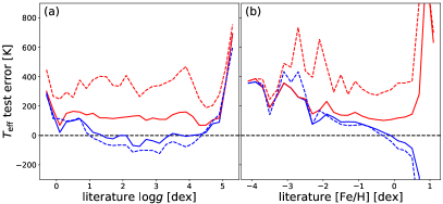
Using the test set with literature values for , , and , Fig. 24 shows how the differences between our temperatures and those in the literature vary with and . Other than for the extreme values, the test errors (RMS and bias) show no significant dependence on . In particular, dwarfs and giants have the same quality of temperature estimates. For , our estimates are strongly overestimated. This might be because our high stars are generally cool, with spectra dominated by molecular absorption which may complicate the estimation of even when dealing with broad-band integrated photometry. Alternatively it’s due to dwarfs being preferentially nearby and thus generally having a low extinction compared to the mean of the training sample, resulting in an overestimation of (see Fig. 13).
The right panel of Fig. 24 shows that the RMS error increases with decreasing metallicity, with the smallest RMS error (and bias) around solar metallicity. In the range our estimates are good, which simply reflects the metallicity distribution in our training sample. Outside this interval, Priam estimates of (and thus the derived FLAME parameters) are more biased. Note that for metal-poor stars, Priam systematically overestimates , which will play a role for halo stars but is probably secondary to the impact of extinction in Fig. 12.
6.2 Stellar types in CMD and HRD
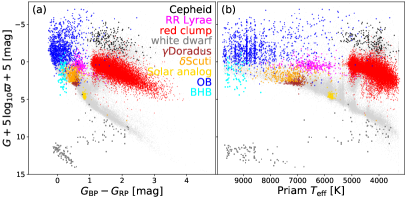
In Fig. 25 we identify stars in our CMDs using classifications from the literature. This demonstrates that different classes of stars appear where we would expect them to.171717Variable stars of course move around in the CMD according to their phase. The photometry is averaged over many observation epochs, so the positions here correspond to some kind of time average which may not be very representative. However, Fig. 25b makes it clear that our temperature estimates are unreliable for highly extincted stars, which is the case for these red clump stars. This is consistent with the fact that we assume low extinction when estimating in Priam. This restriction was necessary given the strong – degeneracy in the colours used (see section 2.1). Note also that even most of the white dwarfs appear in the right location in Fig. 25b, even though we excluded all white dwarfs from the Priam training sample. There are, however, quite a few white dwarfs that fall between the main, obvious white dwarf sequence and the lower envelope of the main sequence. We see this in both panels of Fig. 25, so it is not an artefact of the Apsis results but rather some problem with the photometry (e.g. blending with a low-mass companion in an unresolved binary system).
6.3 Temperature estimates for very hot and very cool stars
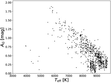
What happens to stars which have true outside the training interval 3000K–10 000K? Intuitively, we would expect that hotter stars are assigned temperatures just below 10 000K, whereas cooler stars are assigned temperatures just above 3000K. This can be seen in Fig. 25b, where most of the OB stars indeed have estimates above 8000K up to the limit of the grid. However, there are also a few cases where OB stars are assigned significantly lower temperatures. Priam infers high extinctions for these (see Fig. 26). Since OB stars often reside in regions with substantial dust, the resulting reddening makes them appear cooler, leading Priam to assign a lower (as explained earlier). The univariate nature of ExtraTrees is a limitation here, since it prevents a high extinction estimate from being a signal that observed colours may be substantially reddened. (We will use multivariate models in Gaia DR3; see section 8.) Furthermore, the degeneracy between and cannot lead to overestimating OB star extinctions by much, since there are no other models that are intrinsically even bluer that these.
At the lower end, we have eight stars in our test set with literature estimates below 3000K. Of these, seven are assigned below 4000K and the eighth is assigned 4120K. The lower limit is obviously better behaved than the upper temperature limit, where extinction is leading to additional confusion.
The inability of ExtraTrees to extrapolate from its training label range of 3000K – 10 000K does not only apply to the median but also to the 16th and 84th percentiles serving as uncertainty estimates. Consequently, the uncertainties cannot appropriately reflect the underestimation of for OB stars, for example.
6.4 Solar analogues and Gaia benchmark stars
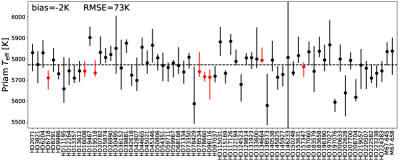
As mentioned in section 5.1, the error in our temperature estimates depends strongly on the temperature distribution of the sample under consideration. Here we look at a sample of 88 solar analogues from Tucci Maia et al. (2016), of which 70 were in our processing and have clean flags. As shown in Fig. 27, most of our estimates are close to the solar value of 5772K (see Table 3). Excluding the eight solar analogues that were part of the training sample for ExtraTrees, the RMS test error for the remaining 62 stars is just 73K (1.3%), which is much smaller than the mean RMS error of 324 K reported in section 5.1. The likely explanation for this excellent performance is that the solar temperature is very close to the mean temperature in our training sample (see Fig. 5), which is where machine learning algorithms usually perform best.
Regarding our uncertainty estimates, we find that the solar temperature is below our lower uncertainty level in 23% of cases, and above the upper uncertainty level for 29% of cases. This agrees with our findings from section 5.1.
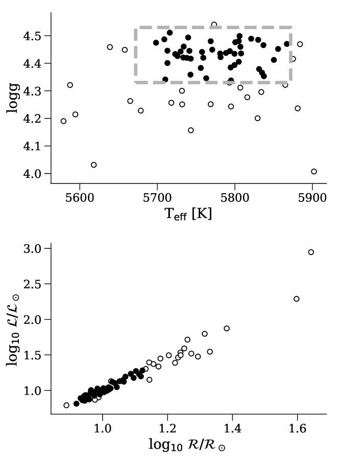
All of the 70 solar analogues found in our catalogue have valid parallaxes and so and were derived. We can estimate their surface gravities () using and assuming solar mass. These are shown in Fig. 28. We refine our selection of solar analogues by requiring to be within 100 K of the Sun and within 0.1 dex. This leaves 46 better analogues, shown as filled circles in Fig. 28. We can see this more clearly in the lower panel of Fig. 28. The importance of adding the parallax, magnitude, and to distinguish between what we consider solar analogues is evident. Using this set of 46 better solar analogues we derive a mean from their and values. By assuming their = , we obtain a mean value of mag for these solar analogues, which is in good agreement with our adopted value for the Sun of mag from section 4.1 (derived in appendix D).
16 of the 34 Gaia benchmark stars (Heiter et al., 2015) are in Gaia DR2 (the missing 18 are too bright for the current processing). All have estimates from Priam: the RMS difference with respect to Heiter et al. (2015) is 230 K, which includes a mean difference of 24 K. However, only 6 of the 16 benchmark stars have parallaxes and thus FLAME results, and the RMS difference of to Heiter et al. (2015) is 13.1%, which includes a mean difference of 3.7%.
6.5 Ensemble extinction at high Galactic latitudes
We can validate our extinction estimates using stars at high Galactic latitudes, , where we expect the true extinction to be close to zero, especially for nearer stars (e.g. Schlegel et al., 1998; Schlafly et al., 2015). However, as our method cannot produce negative extinctions, and given the presence of noise, it is obvious that the average extinction for any ensemble of stars must be larger than zero. Here we study this effect and compare it to our expectations from simulations. We use extinction and reddening estimates for the full sample which is not available to the reader due to the filtering of outliers described in this section. We also derive global uncertainty estimates for and .
Fig. 29a shows the distribution of for high Galactic latitude stars (black histogram). The distribution is clearly peaked at zero extinction and roughly follows an exponential distribution (see below). In particular, 74% of these high Galactic latitude stars have extinctions below 0.5 mag (in the Gaia DR2 sample 82% of them have mag due to the removal of outliers). Nonetheless, there is a prominent tail extending to extinction values as large as mag. We also show simulation results (orange histogram) where we applied Priam to synthetic sources from PARSEC which had zero extinction. This produces a similarly heavy tail (note that the distribution is hardly changed if we add typical Gaia noise to the simulated photometry).

The origin of this heavy tail is revealed by Fig. 29b, where two pronounced groups of stars with large extinctions (“outliers”) emerge, one around mag and the other at mag. These outliers, while relatively few in number (note the colour scale), are assigned unreasonably large extinctions. We see these in Fig. 29c as the two yellow patches on the upper envelope of the main sequence, one around mag and the other around mag. Both cases are a consequence of the strong degeneracy of extinction with temperature: The observed red colour can be incorrectly interpreted as an intrinsically bluer and brighter star being made redder and fainter through extinction. We see high extinction in those regions of the CMD where such hotter but extincted stars in the Priam training set can appear. The same behaviour occurs in the simulation shown for comparison in Fig. 29a, where we see a long tail to high extinctions. We conclude that these outliers are the result of an unfortunate alignment of the extinction vector with the astrophysically allowed states in the CMD as defined by the PARSEC training sample. This is a fundamental limitation imposed by having only three broad optical bands (, , ). The BP/RP spectra should enable us to largely overcome this problem in Gaia DR3 (see section 8).
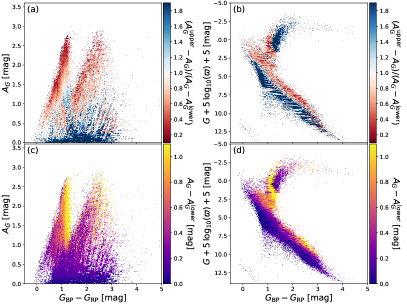
These outliers were removed from the Gaia DR2 catalogue according to the following criteria. The degeneracies are caused by model stars with different extinctions and reddenings (and different stellar parameters) having the same apparent magnitudes. In such a case, the ExtraTrees ensemble provides a wide range of estimates over all these degenerate states, since it cannot distinguish among them. As our uncertainty estimates are a measure of this spread, such outliers will have large uncertainty intervals. Thus, Gaia DR2 only retains estimates of and for sources which satisfy the following conditions
| (8) | ||||
| (9) | ||||
| (10) | ||||
| (11) |
and refer to the 16th and 84th percentiles respectively and likewise for and . The first two filters are justified by Fig. 30. A similar figure justifying the latter two can be found in the online documentation. Of the 161 million sources with extinctions from Apsis, 88 million pass these criteria and so have extinctions in Gaia DR2. While this removes most of the outliers, it is of course not perfect. Unfortunately, the filters also remove many stars on the main sequence turn-off and the lower giant branch. The complete CMD before applying these filters is shown in Fig. 31, which should be compared directly to Fig. 19d to see the impact of the filtering.
We now return to the sample of high Galactic latitude stars () with this filtering applied. This results in the distribution shown in Fig. 32. It agrees very well with an exponential distribution of mean 0.30 mag and its standard deviation from zero extinction, , is 0.46 mag. The fact that Fig. 32 is largely consistent with an exponential distribution is important, because this suggests these high Galactic extinction values are consistent with truly zero with random noise according to information theory: if AG values are pure noise then its distribution follows its maximum entropy distribution, and with a positivity constraint this distribution is an exponential (e.g. Dowson & Wragg, 2006). If the true extinction of high Galactic latitude stars is zero, then our method will infer a positive value which is just noise; the distribution over these extinctions must therefore be the maximum entropy distribution for a non-negative real-valued quantity, which is an exponential. Since Fig. 32 is very consistent with an exponential distribution, this is evidence that is pure noise for high Galactic latitude stars.181818The agreement with an exponential is not perfect, as is obvious from Fig. 32b. Possible explanations are an imperfect removal of outliers and genuine extinction features at high Galactic latitudes such as young clusters.
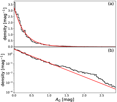
The reddening is also largely consistent with an exponential, of mean 0.15 mag and a standard deviation about zero, , of 0.23 mag.
From these results we obtain “global” uncertainty estimates for and of 0.46 mag and 0.23 mag, respectively. These are slightly larger than our comparisons to literature values of and from Table 6, but we take these as estimates of our overall uncertainties.
6.6 Red clump stars
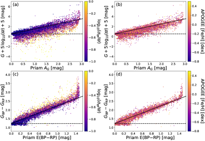
As discussed earlier (section 5.2), our estimates of and show a large RMS error on a test sample, so are generally only useful when combined in an ensemble. We examine here our extinction estimates for red clump stars from Bovy et al. (2014) in order to derive a global uncertainty estimate for and . We found 18 957 of their red clump stars in the Gaia DR2 sample with , whereby 15 876 still had extinction and reddening estimates after applying the filters from equations (8)–(11). Using PARSEC models (Bressan et al., 2012) with , , and evolutionary stage “4”, we estimate that red clump stars reside in a box with a central absolute magnitude of mag (which agrees with Ruiz-Dern et al., 2017) and a central colour of mag. In Fig. 33 panels a and b we plot the observable computed from the Gaia data (which is equal to ), against our estimate of . For 12 127 red clump stars with parallax uncertainties below 20%, we indeed find a relation that is consistent with the absolute magnitude inferred from the PARSEC models. Likewise, if we plot the observed colour against our estimated , we also find results that are consistent with the intrinsic colour inferred from PARSEC (Fig. 33 panels c and d). Even though many red clump stars have APOGEE metallicity and abundance estimates (Alam et al., 2015) that differ from solar metallicity, thus violating our model assumptions from section 3.3, there are no obvious biases. Using the method described in Appendix C, we find that our estimates of and differ from the observables and by about 0.21 mag and 0.09 mag, respectively. These uncertainty estimates are substantially smaller than the global uncertainty estimates of 0.46 mag for and 0.23 mag for that we obtained from high Galactic latitude stars in section 6.5. This suggests that our extinction and reddening estimates work better for red clump stars. Furthermore, we find that our estimates of and are unbiased, since for panels b and d in Fig. 33, the resulting intercept estimates (obtained from appendix C) of 0.27 mag for and 1.22 mag for agree very well with the absolute magnitude and intrinsic colour inferred from PARSEC models. Note that the red clump selection by Bovy et al. (2014) may also contain a few RGB stars, contaminating our analysis. Furthermore, there is an intrinsic spread in the absolute magnitude and colour of the red clump. We neglect this, so our uncertainty estimates of and for red clump stars are conservatively large. Finally, note that the sharp upturn around in Fig. 33d suggests that some of the red clump stars may be subject to such strong extinction that they are not covered by our model grid (which extends to mag).
6.7 Dust towards Galactic clusters and nebulae
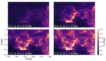
Schlafly et al. (2015) have investigated the three-dimensional structure of the line-of-sight extinction for the Orion nebula. We show in Fig. 34 our estimates in the same way as Fig. 2 of Schlafly et al. (2015). Each cell shows the mean extinction over the distance range given. As noted in appendix E, this is likely to be an overestimate when the true extinction is low. The agreement is nonetheless striking, although we are missing the fainter stars due to the limit in our processing.
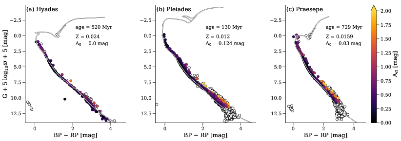
To further assess the quality of our estimates of dust attenuation, we studied the colour–absolute magnitude diagrams of some Galactic star clusters. Fig. 35 shows three examples, with members taken from Gaia Collaboration et al. 2018a who selected them based on their spatial positions and proper motions. The plot shows good agreement with isochrone models of matching age, metallicity, and extinction from Castellani et al. (2002). The colour scale shows the extinction estimates from Priam. The sequences above and parallel to the main sequence in both clusters are presumably binaries. These tend to have larger (overestimated) extinctions. As binaries have slightly redder colours than single stars of the same brightness due to the generally lower mass companion, yet have the same parallax, Priam – assuming all stars to be single – interprets their redder colours to be a result of extinction. (Binary stars will receive explicit treatment in future Gaia data releases; see section 8.)
We show in appendix E that, because our extinction estimates are non-negative, the mean of a sample of stars is often a biased estimator of the true (assumed common) extinction. We can instead use a likelihood function for each star which respects this non-negativity, namely a truncated Gaussian. When we do this, the maximum of the likelihood for the set of cluster members is mag for the Hyades, mag for the Pleiades, and mag for Praesepe (the uncertainties refer to the 16th and 84th percentiles on the likelihood). These cluster extinction estimates are in very good agreement with the values from Castellani et al. (2002) and Taylor (2006), listed in Fig. 35, for the Pleiades and Praesepe clusters. Our estimate for the Hyades, in contrast, is much larger than the literature value. As discussed in appendix E, we suspect this is just a combination of bad luck and a relatively small number of members for precisely locating the maximum of the likelihood. Finally, we note that even within our clean sample, our results in clusters may suffer from photometric errors induced by crowding.
6.8 Validation of radii and luminosities with seismology, interferometry, and surveys of nearby stars
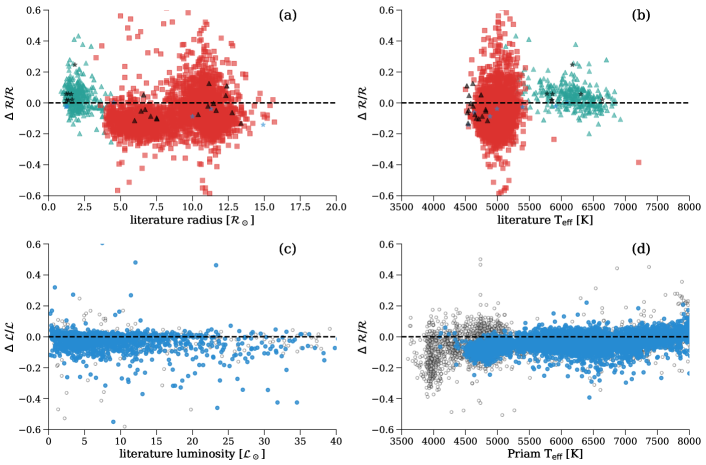
To validate the results for FLAME, we compare the derived radii and luminosities with those from a selection of external catalogues. These are shown in Fig. 36, whereby the targets are mostly bright () and nearby ( pc). The top panels compare the radii from a compilation of asteroseismic and interferometric references as a function of literature radii (panel a) and (panel b). For the less evolved stars ( 3.0 ) the FLAME radii are slightly overestimated, but the differences are consistent with zero considering the radius uncertainties for this range (Fig. 9), due to the differences in the adopted temperature scales. The green triangles represent radii from automatic asteroseismic analysis using scaling relations, where typical uncertainties in the radius can be 5% and the actual values of the radii are rather sensitive to the input (see Chaplin et al. 2014). For this sample we also find a systematic trend in the radii which increases with decreasing (panel b). This suggests that the differences in the radii arises from the different temperature scales used. The other stars in this less evolved sample range have been studied in much finer detail using interferometry or detailed asteroseismic analysis (black and blue stars). In these cases, the literature radii are much less sensitive to the adopted . For these better-studied stars, we do find much better agreement with the FLAME radii (), with no significant differences as a function of .
The largest sample in this figure is that from Vrard et al. (2016), who studied red giants using asteroseismic scaling relations in an automatic manner. For the giants, typical uncertainties in the asteroseismic radii are of the order 7–10% and the radii are sensitive to the adopted . As explained earlier, we ignore interstellar extinction, and thus the luminosities will be systematically underestimated. This is particularly problematic for giants which are more distant, as extinction could be non-negligible. However, for a fixed a smaller luminosity implies a smaller radius. In most cases we see that the radii are underestimated (negative differences). However, in the range there is a large scatter around zero (there are many overestimated radii too). This zero offset is a direct result of the cancellation effects of the adopted temperature scales and of ignoring extinction. For this sample of stars, we find systematically lower with Priam, where the typical differences are between –5% and –1%. As a consequence, for fixed luminosity, the radius will be overestimated by FLAME. As with the main sequence stars, the interferometric sample (blue stars) and the giants in NGC 6819 (black triangles), which were studied in much finer detail, agree with the FLAME radii to within 10%, and show no trend in their differences as a function of radius or .
In the lower panels of Fig. 36 we compare our estimates of and with those derived from external analyses based on photometric measurements. The left panel (c) compares our luminosities with those derived from the bolometric flux estimates from Casagrande et al. (2011). We also compared our radii using their bolometric flux and temperature measurements (not shown). We obtain a negligible mean difference in the luminosities and radii which can be rectified by changing the by a few mmag (see appendix D). We find a dispersion below %, suggesting no unknown systematic effects in our results. In the lower right panel (d) we compare FLAME radii with those derived from predicted angular diameters from Bourges et al. (2017). Again we find a mean offset in the differences close to zero and a dispersion about this mean of less than 10%. In both figures, the blue filled circles represent a subset of these data which fulfil the criteria Priam , , Gaia , and pc. These were used to test the discussed in appendix D. The open black circles are stars retrieved in our validation data which don’t fulfil these criteria.
7 Using the data
In this work we have, independently for each source, inferred five parameters from three partially degenerate flux measurements and (for all but ) a parallax. This has necessarily demanded a number of extreme simplifications and assumptions. The data should therefore be used with great care. We recommend always using the flags, defined in appendix B, to filter out poorer data. In particular, for astrophysical analyses, we recommend only using parameters for stars in the clean sample (defined in that appendix). When using extinctions, luminosity, and radii users may also want to only select stars with small fractional parallax uncertainties (Fig. 19 gives an example of the impact of this filtering on the CMD.)
7.1 Limitations and caveats
The following caveats should be kept in mind.
-
1.
All sources are treated as single stars. We do not perform source classification and our processing does not make use of external classifications. We do not filter out results for sources we know from other data to be galaxies, unresolved binaries, etc.
-
2.
The training sample for of ExtraTrees contains stars with a certain range of (low) extinctions (see section 3.2). The estimates will be systematically too low when the true extinction is significantly below this range (e.g. in the halo). Likewise, estimates will be systematically too high when the extinction is above this range. One manifestation of this is a systematic trend in temperature errors (from comparison to literature estimates) with Galactic latitude (see Fig. 12). Hot stars with high extinction get estimates that are systematically too low (see Fig. 18). See also Fig. 11e.
-
3.
For estimation, ExtraTrees was only trained on the range 3000K–10 000K. Stars which are truly hotter or cooler will therefore be systematically under- or overestimated. However, for and estimation, ExtraTrees was trained on PARSEC models with mag and 2500 K 20 000 K. While we cannot get estimates from those models, we still get reliable extinction and reddening estimates for intrinsically blue sources such as OB stars.
- 4.
-
5.
The (empirical) training sample lacks low metallicity stars, so systematic errors in can be expected for truly low metallicity stars. The same can be said for the extinction estimates, as our (synthetic) training sample is solar metallicity.
-
6.
As we use three broad optical bands, our estimates of and are highly degenerate with our estimates. This leads to unreliable extinction and reddening estimates in parts of the CMD (see section 6.5).
-
7.
Our extinction estimates are strictly non-negative, with uncertainties of similar size to the estimate itself. Hence neither nor can be considered as a Gaussian random variable, not even approximately. The likelihood (probability density) is intrinsically skewed, which is why we report 16th and 84th percentiles to reflect the uncertainty. As explained in appendix E, a truncated Gaussian is a more appropriate likelihood model for the extinctions. The non-negativity can feign a systematic overestimation of extinction in regions where very low extinction is expected, such as at high Galactic latitudes (section 6.5) or for some stellar clusters (section 6.7). As we show in appendix E, the mean extinction in such regions is a poor estimator of the true extinction.
-
8.
The estimates of and generally have such large uncertainties that their usefulness for individual stars is limited. These estimates should generally only be used statistically, by applying them to ensembles of stars. The central limit theorem applies despite the non-negativity, ensuring that the variance in the mean of a sample will drop as , even though the mean may be a biased estimator. The Galactic extinction map (Fig. 21) and the Orion map (Fig. 34) suggest that mean extinctions are reliable. The –extinction degeneracy in the photometric data nonetheless mean that some extinctions are quite erroneous, although many of these were removed by the cuts applied by equations 8 to 11.
-
9.
The extinction estimates satisfy . This is a consequence of the models which we are using (see Fig. 7).
-
10.
Our extinction estimates are based on PARSEC 1.2S models with extinction assuming fixed . Using a different , a different extinction law, or a different set of stellar models may lead to systematic differences compared to our current estimates.
- 11.
-
12.
Stellar clusters, in particular globular clusters, are crowded regions where the integrated photometry is sometimes compromised. The BP and RP photometry are obtained by integrating over an area of arcsec2. As the two Gaia fields-of-view are projected onto a common focal plane, sources can overlap even in low density regions. For crowding and other reasons, users may want to additionally filter out sources according to the “BP/RP flux excess” (see Evans et al. 2018).
-
13.
Parallaxes are used to estimate , , , and , by giving a distance somewhat naively as (see Bailer-Jones, 2015; Luri et al., 2018). Sources without positive parallaxes therefore have no estimates of these parameters, and those with large fractional parallax uncertainties () will have particularly noisy estimates of these parameters. This applies in particular to distant and/or faint stars. We recommend only using estimates for these parameters for stars with fractional parallax uncertainties of 20% or less.
-
14.
The uncertainties in the and are most likely underestimated. The luminosity may suffer from a systematic error based on the adoption of the value of (see appendix D), although we estimate this to be within 0.1 mag. Luminosity will also be systematically underestimated for extincted stars, since we assumed extinction to be zero when inferring the absolute magnitude. As is derived directly from and , both of these effects also impact the radius estimates, albeit to a smaller degree (see section 5.4).
The application and implication of the above guidelines is illustrated in the following sections.
7.2 Selection of targets for interferometry

Measurements of apparent diameters of stars with ground-based interferometry play a crucial role for direct estimation of stellar temperatures (e.g. Heiter et al., 2015) or the validation of asteroseismic radii (e.g. White et al., 2013). Long-baseline optical interferometry can reliably measure angular diameters as small as 0.2 (e.g. Boyajian et al., 2015). Our results may be used to select potential targets for such interferometric observations. We suggest the following selection criteria:
| (12) | |||
| Priam flag 0100001 or 0100002 |
The cut on relative parallax uncertainty is obviously necessary in order to obtain a reliable distance estimate to infer a reasonably accurate diameter from the FLAME radius. We find 213 139 targets satisfying these criteria. As shown in Fig. 37, all of these are brighter than . Most of these targets are cool giants but some are main sequence stars. Since and the flux scales as , we expect , where the constant depends on , among other things. This scaling is confirmed by Fig. 37a. The diagonal stripes are due to the FLAME radius estimation relying on Priam temperatures which are based on a training sample with a inhomogeneous temperature distribution (see Fig. 18). Gaia DR2 is incomplete at the bright end (Evans et al., 2018), which unfortunately reduces the overlap with potential interferometric targets.
7.3 Selection of red clump candidates
The red clump is prominent in the de-reddened CMD in Fig. 19d. We suggest the following selection criteria to isolate candidates for red clump stars:
| (13) | |||
This selection produces 1 877 297 candidates. Of the 19 937 red clump candidates from Bovy et al. (2014), 19 240 are in Gaia DR2 and have , and 14 510 of these pass the astrometry criterion above. The cuts in intrinsic colour and absolute magnitude are then passed by 4415 known red clump stars.
7.4 Selection of solar analogue candidates
Based on the results from Fig. 27, we adopt the following selection criteria for solar analogue candidates:
| (14) | |||
| Priam flag 0100001 or 0100002 |
This selection results in 124 384 candidates for . However, we caution that this selection probably has significant contamination from non-solar-like stars with poorly estimated temperatures.
8 Looking ahead to the third Gaia data release
The broad band fluxes used in this paper were derived from Gaia’s low resolution spectrograph BP/RP. The full spectra are not made available in Gaia DR2 due to insufficient calibration at this stage in the data processing. For the next data release – Gaia DR3 – we plan to infer more detailed and more precise astrophysical parameters using these spectra.191919Initial results with preliminary BP/RP spectra in an empirically-trained algorithm show very promising results when comparing to the literature, not only for , but also for and . This will be done using further algorithms within the astrophysical parameter analysis system (Apsis), of which the algorithms Priam and FLAME discussed in the present paper are just a small part. For details of Apsis see Bailer-Jones et al. (2013).
The full BP/RP spectrophotometry permit estimates of both the effective temperature and the extinction without the need to use parallaxes. Simulations show that these spectra should also allow good estimates of and (Bailer-Jones, 2010, 2011; Liu et al., 2012). A separate algorithm will use the spectra together with the parallaxes to estimate , , , and together with luminosity and distance, self-consistently. This should provide a more reliable distance estimate than using only the parallax (e.g. Astraatmadja & Bailer-Jones, 2016), especially for sources beyond a few kpc. The radius estimates will then be more precise, and using the estimate we will also be able to infer mass. Using evolutionary tracks we plan also to release estimates of stellar ages for some types of stars.
Independent estimates of stellar parameters for bright stars will be possible using the high resolution radial velocity spectrograph (Gaia Collaboration et al., 2016), which gives information sensitive to , , , and in the region 845–872 nm (Recio-Blanco et al., 2016). Further algorithms in Apsis will be dedicated to exploring ultra cool dwarfs (Sarro et al., 2013), emission line stars, and unresolved binary stars.
In the future we will no longer have to treat all sources as single stars. The Discrete Source Classifier in Apsis will classify sources using not only BP/RP (Bailer-Jones et al., 2008), but also the astrometry and apparent magnitude. Quasars and unresolved galaxies identified in this way will be treated by source-specific algorithms (Delchambre, 2018; Bellas-Velidis et al., 2012) to derive redshift, morphology type, etc. In addition to classifying source-by-source, we also plan some global analyses to identify sources which don’t fit into our supervised classification schemes (e.g. Fustes et al., 2013), and to do large scale statistical cluster analyses to find empirical relations between sources. How much of this can be released in Gaia DR3 depends in part on the quality of the data and calibrations at the next stage of the data processing.
9 Summary
We have presented the methods used for estimating stellar parameters and line-of-sight extinctions in Gaia DR2, as well as an analysis and validation of the results. The parameter estimates are based on very limited input data, namely the parallax and the integrated photometry in three bands, , , and . More detailed and accurate parameters should be released in Gaia DR3 once the BP/RP spectrophotometry and RVS spectra can be used.
Broadly speaking, we can estimate effective temperature with an accuracy of about 324 K in the range 3000K to 10 000K. For solar analogues and Gaia benchmark stars (Heiter et al., 2015), we achieve RMS errors as low as 75K and 230K, respectively. Our test and training samples were drawn from the same parent distribution, which are not necessarily representative of all stellar populations. For the same reason, there are some systematic misestimations of , e.g. for sources with very low or very high extinctions (see Fig. 11e and Fig. 12). Likewise, there appear to be systematic trends with the actual temperature (Fig. 11c), the colour (Fig. 11f) and with metallicity (Fig. 24b). These figures attempt to quantify these systematics, but they are not included in the 324K uncertainty estimates which, by definition, quantify only random errors. The reported 16th and 84th percentiles appear to be consistent with differences to literature estimates when also accounting for literature uncertainty estimates.
The line-of-sight extinction and the reddening are estimated with global uncertainties of 0.46 mag and 0.23 mag, respectively (section 6.5). Better estimates can be achieved for red clump stars (section 6.6). Note that is the extinction in the G-band rather than an extinction parameter, so also depends on the spectral energy distribution (and thus ) of the star. Thus a given amount of dust can correspond to different values of , depending on the type of star. Given only three broad optical bands as input data, there are obviously strong degeneracies; we have explored the systematics these can introduce into our extinction estimates. After applying quality cuts to remove outliers, there is no evidence for further biases. Nevertheless, with such large random errors and are of limited use for individual stars. However, and can be used statistically on a set of stars, for example to apply a dust correction in the colour-magnitude diagram. Given the degeneracy, for our estimations and our subsequent estimations of bolometric luminosity and radius , we have assumed the sources have zero (or at least low) extinction.
Adopting a bolometric correction offset determined empirically, we have estimated to an accuracy of about 15% and to about 10% (RMS errors), again without significant systematics.
Given the limited input data, we necessarily rely on a number of assumptions and simplifications. We list some known limitations of our results in section 7.1. These must be considered when using our data products. We recommend that only our clean sample be used (appendix B). For better estimates of extinction, users may want to only use stars with some maximum fractional parallax uncertainty (see Fig. 19 for an example of this).
Finally, we emphasise again that the objective of this work was to provide stellar parameter estimates using Gaia data only. Substantially better results are likely achievable when combining with other data, such as GALEX (Morrissey et al., 2007), PanSTARRS (Chambers et al., 2016) or WISE (Cutri et al., 2014). McDonald et al. (2017) and Stevens et al. (2017) have attempted that already with Gaia DR1 data, although they faced severe problems with cross-matching the different catalogues due to the high spatial resolution of the Gaia catalogue. Great care must be exercised when using multi-catalogue spectral energy distributions resulting from such cross-matches, since the passbands are not always well defined for some photometric systems (e.g., APASS; Henden et al. 2016).
Although limited in precision and accuracy, our results should nonetheless be useful as the largest, all-sky catalogue of homogeneously-inferred stellar parameters published to date, and the first to use parallaxes on a large scale.
Acknowledgements.
For their constructive comments on the manuscript we thank Carine Babusiaux, Anthony Brown, Ron Drimmel, Yves Frémat, Carme Jordi, Jan Rybizki, Antonella Vallenari, and the anonymous referee. We thank Floor van Leeuwen for providing membership lists of stellar clusters in Gaia DR2. This work is based on data from the European Space Agency (ESA) mission Gaia (https://www.cosmos.esa.int/gaia), processed by the Gaia Data Processing and Analysis Consortium (DPAC, https://www.cosmos.esa.int/web/gaia/dpac/consortium). Funding for the DPAC has been provided by national institutions, in particular the institutions participating in the Gaia Multilateral Agreement. Funding specifically for the DPAC work in this paper has been provided by the DLR (German space agency) via grants 50 QG 0602, 50 QG 1001, and 50 QG 1403. AJK acknowledges support by the Swedish National Space Board (SNSB). This research has made extensive use of IPython (Pérez & Granger, 2007), matplotlib (Hunter, 2007), and Vaex (Breddels, 2017).References
- Alam et al. (2015) Alam, S., Albareti, F. D., Allende Prieto, C., et al. 2015, ApJS, 219, 12
- Astraatmadja & Bailer-Jones (2016) Astraatmadja, T. L. & Bailer-Jones, C. A. L. 2016, ApJ, 833, 119
- Bailer-Jones (2010) Bailer-Jones, C. A. L. 2010, MNRAS, 403, 96
- Bailer-Jones (2011) Bailer-Jones, C. A. L. 2011, MNRAS, 411, 435
- Bailer-Jones (2015) Bailer-Jones, C. A. L. 2015, PASP, 127, 994
- Bailer-Jones et al. (2013) Bailer-Jones, C. A. L., Andrae, R., Arcay, B., et al. 2013, A&A, 559, A74
- Bailer-Jones et al. (2008) Bailer-Jones, C. A. L., Smith, K. W., Tiede, C., Sordo, R., & Vallenari, A. 2008, MNRAS, 391, 1838
- Basu et al. (2011) Basu, S., Grundahl, F., Stello, D., et al. 2011, ApJ, 729, L10
- Bellas-Velidis et al. (2012) Bellas-Velidis, I., Kontizas, M., Dapergolas, A., et al. 2012, Bulgarian Astronomical Journal, 18, 020000
- Bishop (2006) Bishop, C. M. 2006, Pattern Recognition and Machine Learning (Springer)
- Bourges et al. (2017) Bourges, L., Mella, G., Lafrasse, S., et al. 2017, VizieR Online Data Catalog, 2346
- Bovy et al. (2014) Bovy, J., Nidever, D. L., Rix, H.-W., et al. 2014, ApJ, 790, 127
- Boyajian et al. (2015) Boyajian, T., von Braun, K., Feiden, G. A., et al. 2015, MNRAS, 447, 846
- Boyajian et al. (2013) Boyajian, T. S., von Braun, K., van Belle, G., et al. 2013, ApJ, 771, 40
- Breddels (2017) Breddels, M. A. 2017, in IAU Symposium, Vol. 325, IAU Symposium, 299–304
- Bressan et al. (2012) Bressan, A., Marigo, P., Girardi, L., et al. 2012, MNRAS, 427, 127
- Cardelli et al. (1989) Cardelli, J. A., Clayton, G. C., & Mathis, J. S. 1989, ApJ, 345, 245
- Casagrande et al. (2011) Casagrande, L., Schoenrich, R., Asplund, M., et al. 2011, VizieR Online Data Catalog, 353
- Castellani et al. (2002) Castellani, V., Degl’Innocenti, S., Prada Moroni, P. G., & Tordiglione, V. 2002, MNRAS, 334, 193
- Castelli & Kurucz (2003) Castelli, F. & Kurucz, R. L. 2003, in IAU Symposium, Vol. 210, Modelling of Stellar Atmospheres, ed. N. Piskunov, W. Weiss, & D. Gray
- Chambers et al. (2016) Chambers, K. C., Magnier, E. A., Metcalfe, N., et al. 2016, ArXiv e-prints 1612.05560
- Chaplin et al. (2014) Chaplin, W. J., Basu, S., Huber, D., et al. 2014, VizieR Online Data Catalog, 221
- Creevey et al. (2017) Creevey, O. L., Metcalfe, T. S., Schultheis, M., et al. 2017, VizieR Online Data Catalog, 360
- Cutri et al. (2014) Cutri, R. M., Wright, E. L., Conrow, T., et al. 2014, VizieR Online Data Catalog, 2328
- de Bruijne (2012) de Bruijne, J. H. J. 2012, Ap&SS, 341, 31
- Delchambre (2018) Delchambre, L. 2018, MNRAS, 473, 1785
- Deming (1943) Deming, W. 1943, Statistical Adjustment of Data, Dover books on elementary and intermediate mathematics (Dover Publ. Incorporated)
- Deng et al. (2012) Deng, N., Tian, Y., & Zhang, C. 2012, Support Vector Machines: Optimization Based Theory, Algorithms, and Extensions, 1st edn. (Chapman & Hall/CRC)
- Dowson & Wragg (2006) Dowson, D. & Wragg, A. 2006, IEEE Trans. Inf. Theor., 19, 689
- Evans et al. (2018) Evans, D., Riello, M., De Angeli, F., et al. 2018, A&A
- Fuller (2009) Fuller, W. 2009, Measurement Error Models, Wiley Series in Probability and Statistics (Wiley)
- Fustes et al. (2013) Fustes, D., Manteiga, M., Dafonte, C., et al. 2013, A&A, 559, A7
- Gaia Collaboration et al. (2018a) Gaia Collaboration, Babusiaux, C., & et al. 2018a, A&A
- Gaia Collaboration et al. (2018b) Gaia Collaboration, Brown, A., Vallenari, A., Prusti, T., & de Bruijne, J. 2018b, A&A
- Gaia Collaboration et al. (2016) Gaia Collaboration, Prusti, T., de Bruijne, J. H. J., et al. 2016, A&A, 595, A1
- Geurts et al. (2006) Geurts, P., Ernst, D., & Wehenkel, L. 2006, Mach. Learn., 63, 3
- Gustafsson et al. (2008) Gustafsson, B., Edvardsson, B., Eriksson, K., et al. 2008, A&A, 486, 951
- Heiter et al. (2015) Heiter, U., Jofré, P., Gustafsson, B., et al. 2015, A&A, 582, A49
- Henden et al. (2016) Henden, A. A., Templeton, M., Terrell, D., et al. 2016, VizieR Online Data Catalog, 2336
- Huber et al. (2014) Huber, D., Silva Aguirre, V., Matthews, J. M., et al. 2014, ApJS, 211, 2
- Hunter (2007) Hunter, J. D. 2007, Computing In Science & Engineering, 9, 90
- Jordi et al. (2010) Jordi, C., Gebran, M., Carrasco, J. M., et al. 2010, A&A, 523, A48
- Kleinman et al. (2013) Kleinman, S. J., Kepler, S. O., Koester, D., et al. 2013, ApJS, 204, 5
- Kordopatis et al. (2013) Kordopatis, G., Gilmore, G., Steinmetz, M., et al. 2013, AJ, 146, 134
- Lallement et al. (2014) Lallement, R., Vergely, J.-L., Valette, B., et al. 2014, A&A, 561, A91
- Ligi et al. (2016) Ligi, R., Creevey, O., Mourard, D., et al. 2016, VizieR Online Data Catalog, 358
- Lindegren et al. (2018) Lindegren, L., Hernández, J., Bombrun, A., et al. 2018, A&A
- Liu et al. (2012) Liu, C., Bailer-Jones, C. A. L., Sordo, R., et al. 2012, MNRAS, 426, 2463
- Luo et al. (2015) Luo, A.-L., Zhao, Y.-H., Zhao, G., et al. 2015, Research in Astronomy and Astrophysics, 15, 1095
- Luri et al. (2018) Luri, X., Brown, A., Sarro, L., et al. 2018, A&A
- Martell et al. (2017) Martell, S. L., Sharma, S., Buder, S., et al. 2017, MNRAS, 465, 3203
- McDonald et al. (2017) McDonald, I., Zijlstra, A. A., & Watson, R. A. 2017, MNRAS, 471, 770
- Morrissey et al. (2007) Morrissey, P., Conrow, T., Barlow, T. A., et al. 2007, ApJS, 173, 682
- O’Donnell (1994) O’Donnell, J. E. 1994, ApJ, 422, 158
- Pandey et al. (2003) Pandey, A. K., Upadhyay, K., Nakada, Y., & Ogura, K. 2003, A&A, 397, 191
- Pérez & Granger (2007) Pérez, F. & Granger, B. E. 2007, Computing in Science and Engineering, 9, 21
- Pickles (1998) Pickles, A. J. 1998, PASP, 110, 863
- Ramírez-Agudelo et al. (2017) Ramírez-Agudelo, O. H., Sana, H., de Koter, A., et al. 2017, A&A, 600, A81
- Recio-Blanco et al. (2016) Recio-Blanco, A., de Laverny, P., Allende Prieto, C., et al. 2016, A&A, 585, A93
- Riello et al. (2018) Riello, M., De Angeli, F., Evans, D., et al. 2018, A&A
- Rodrigues et al. (2014) Rodrigues, T. S., Girardi, L., Miglio, A., et al. 2014, MNRAS, 445, 2758
- Ruiz-Dern et al. (2017) Ruiz-Dern, L., Babusiaux, C., Arenou, F., Turon, C., & Lallement, R. 2017, ArXiv e-prints 1710.05803
- Sarro et al. (2013) Sarro , L. M., Berihuete, A., Carrión, C., et al. 2013, A&A, 550, A44
- Sarro et al. (2016) Sarro , L. M., Debosscher, J., De Ridder, J., et al. 2016, Technical Note GAIA-C7-TN-SVO-LSB-015
- Sartoretti et al. (2018) Sartoretti, P., Katz, D., Cropper, M., et al. 2018, A&A
- Schlafly et al. (2015) Schlafly, E. F., Green, G., Finkbeiner, D. P., et al. 2015, ApJ, 799, 116
- Schlegel et al. (1998) Schlegel, D. J., Finkbeiner, D. P., & Davis, M. 1998, ApJ, 500, 525
- Simón-Díaz et al. (2011) Simón-Díaz, S., Castro, N., Garcia, M., Herrero, A., & Markova, N. 2011, Bulletin de la Societe Royale des Sciences de Liege, 80, 514
- Simón-Díaz et al. (2017) Simón-Díaz, S., Godart, M., Castro, N., et al. 2017, A&A, 597, A22
- Sirko et al. (2004) Sirko, E., Goodman, J., Knapp, G. R., et al. 2004, AJ, 127, 899
- Soubiran et al. (2014) Soubiran, C., Lecampion, J., & Chemin, L. 2014, Technical Note GAIA-C6-TN-LAB-CS-011-2
- Stevens et al. (2017) Stevens, D. J., Stassun, K. G., & Gaudi, B. S. 2017, AJ, 154, 259
- Tammann et al. (2003) Tammann, G. A., Sandage, A., & Reindl, B. 2003, VizieR Online Data Catalog, 340
- Taylor (2006) Taylor, B. J. 2006, AJ, 132, 2453
- Torres (2010) Torres, G. 2010, AJ, 140, 1158
- Tucci Maia et al. (2016) Tucci Maia, M., Ramírez, I., Meléndez, J., et al. 2016, A&A, 590, A32
- Vrard et al. (2016) Vrard, M., Mosser, B., & Samadi, R. 2016, A&A, 588, A87
- White et al. (2013) White, T. R., Huber, D., Maestro, V., et al. 2013, MNRAS, 433, 1262
- Wils et al. (2006) Wils, P., Lloyd, C., & Bernhard, K. 2006, MNRAS, 368, 1757
- Zasowski et al. (2015) Zasowski, G., An, D., & Pinsonneault, M. 2015, in Astrophysics and Space Science Proceedings, Vol. 39, Asteroseismology of Stellar Populations in the Milky Way, ed. A. Miglio, P. Eggenberger, L. Girardi, & J. Montalbán, 83
Appendix A Filtering applied to produce the Gaia DR2 catalogue
Some of the sources processed by Apsis have poor data and cannot yield useful astrophysical parameters. Likewise, our assumptions may sometimes yield invalid results. We therefore apply various filters in post-processing in order to remove some or all parameter estimates. (These filters are applied during the creation of the final catalogue.) Table 7 lists these filters. In addition we always require complete photometry – fluxes available for all of G, BP, and RP – to produce any results, and we only processed sources with . Filters applied by other parts of the processing could remove some sources entirely, regardless of the Apsis results. For more details on filtering, see the online documentation with Gaia DR2. The number of sources in the catalogue with an extant estimate for each parameter is as follows: : 161 497 595; and : 87 733 672; and : 76 956 778.
| condition | parameters excluded | ||||
|---|---|---|---|---|---|
| K or K | |||||
| violation of equations (8)-(11) | |||||
| Priam flag | |||||
Appendix B The Apsis flags
| position | value | meaning |
| A | 0 | parallax value is strictly positive () |
| 1 | parallax value is non-positive () such that extinction estimate does not work | |
| 2 | while the parallax error is mas | |
| B | 0 | both colours are close to the standard locus |
| 1 | below standard locus, i.e., and | |
| 2 | above standard locus, i.e., or | |
| C | 0 | colour is inside union of and extinction training sets |
| 1 | colour is smaller than union of and extinction training sets | |
| 2 | colour is larger than union of and extinction training sets | |
| D | 0 | colour is inside union of and extinction training sets |
| 1 | colour is smaller than union of and extinction training sets | |
| 2 | colour is larger than union of and extinction training sets | |
| E | 1 | input data was gold photometry |
| 2 | input data was silver photometry |
Various flags are written by Apsis during processing to indicate the quality of the input data and/or the results. They have the format XYABCDE, where each letter represents a decimal digit. XY=01 indicates a Priam flag, the values of which are shown in Table 8.
Digits C and D refer to colours in the union of the and extinction training sets. These can be used to remove sources which are unlikely to get good results from Priam. The colour ranges for the separate models are as follows (so a colour selection could be used for the parameter of interest, instead of using these digits in the flags): For : to mag, : to mag. For extinction: : to mag, : to mag.
To get a clean sample of estimates, use only sources with Priam flag values equal to 0100001, 0100002, 0110001, 0110002, 0120001, or 0120002, i.e. A and E can have any value, but B, C, and D are zero. When using for astrophysical analyses, we recommend that this clean sample be used.
For and estimates, the filtering on best Priam flag values has already been applied during the catalog production for Gaia DR2. The user may want to make further cuts to only retain sources with low fractional parallax uncertainties.
After the filtering described in Table 7, only one flag corresponding to FLAME is left in the catalogue (the one beginning with 02), so can be ignored. Since FLAME results depend on , we recommend to only use FLAME results for the clean sample.
Appendix C Uncertainty estimates for and
In section 6.6, we estimate the uncertainties in for red clump stars from Bovy et al. (2014) by comparing our estimate of to the observable (which is equal to ). Likewise, we also compare to the observed colour . In these cases, both variables, call them and , have uncertainties, so a standard least-squares regression would lead to systematically wrong results for the slopes and intercepts in Fig. 33 (e.g. Fuller 2009, section 1.1.1 therein). For each (the observable), the corresponding uncertainty can be obtained by the usual propagation of uncertainties in the G-band flux and the parallax. The uncertainty in and the intercept are our desired estimates. These tell us the uncertainties in and , respectively, and whether we are consistent with the expected absolute magnitude and intrinsic colour of the red clump.
When both and have uncertainties, then in order to obtain an unbiased estimate of , we use a modification of the Deming formalism (e.g. Deming 1943). We introduce the true and true , which satisfy the linear relation
| (15) |
The intercept is the absolute magnitude of the red clump stars for or the intrinsic colour for , which remains a free fit parameter. We set the slope to , since Fig. 33b and d have already established an approximate one-to-one relation between and and we now seek the uncertainty of under this relation. We then estimate the true , the intercept and the uncertainty by minimising
| (16) |
Note the first term which ensures that the likelihood function is normalised, while we fit for the unknown uncertainty . This minimisation has analytic results
| (17) |
and
| (18) |
Unfortunately, there is no analytic solution for . However, a numerical solution can be found easily.
Appendix D Bolometric correction scale
The bolometric correction used to compute the luminosity is calculated on a grid of synthetic stellar spectra for varying values of , , , and . While the variation of the bolometric correction with stellar parameters can be easily evaluated considering any filter band pass, the absolute value can only be derived if we know the absolute magnitude for one source with known bolometric flux and distance. The Sun is the obvious choice. From hereon, we refer to this as the offset of the bolometric correction, and this is the value of in equation 7 for the range 4 000 – 8 000 K.
Adopting the previously-mentioned IAU resolution 2015 B2, the Sun’s bolometric magnitude is = 4.74 mag. Given its distance and its measured -band magnitude, , the absolute magnitude is calculated and the is derived: mag (Torres 2010). However, we do not have a measure of , and so we cannot apply these equations directly to determine . Thus to derive the offset to the bolometric correction scale there are four options: (1) estimate from stellar models; (2) use a to conversion; (3) externally calibrate using stars with accurately measured luminosities and radii; (4) use solar twins to measure (see section 6). We chose to adopt solution (3) and this is described in detail here. It’s also appropriate given that our estimates are based on empirically trained models.
We derive our bolometric correction offset by comparing our overall estimates of luminosity and radius with those from other studies. This works provided the stars in question have accurately determined extinctions (often taken to be zero). Net offsets can indicate a problem with the offset of the bolometric correction (in our study or in the other studies, or both). We perform this comparison on three samples of stars: (1) the Casagrande et al. (2011) analysis of the Geneva Copenhagen Survey data; (2) the JMMC Catalogue of Stellar Diameters (Bourges et al. 2017); (3) an asteroseismic sample of giant stars from Vrard et al. (2016). For these samples we also selected those stars where Priam and Gaia .
Casagrande et al. (2011) provide bolometric flux and in their catalogue. Using these along with the Gaia parallaxes we calculated stellar radii and luminosities. From this sample we selected the stars within 100 pc ( stars in the sample), 200 pc () and 300 pc () of the Sun, and we imposed . We first compared the Priam with theirs, and by adding an offset to compensate for the differences in our we rederived our radii. This was done to isolate the effect of the . Then we adjusted until we minimized the mean difference between our results (luminosities and rederived radii) and theirs. This resulted in = +0.10, +0.09, +0.09 mag for the three distance cuts respectively.
The JMMC catalogue (Bourges et al. 2017) predicts angular diameters from magnitudes and colours; this is the so-called surface-brightness relation. It is calibrated using interferometric measurements of stellar diameters. We performed the same analysis on this catalogue for stars within 100 pc (), 200 pc (), and 300 pc (). By minimizing the mean differences between the radii we derived a of +0.00, +0.01, and +0.01 mag for the three distance cuts respectively.
The third catalogue we used consists of thousands of giants in the Kepler field analysed using asteroseismology (Vrard et al. 2016). Our validation sample comprises 3355 stars. In this case we can not assume that extinction is zero or negligible. The effect of the bolometric correction offset and extinction for deriving is degenerate. Thus we are required to assume a mean extinction for these stars if we wish to estimate . We adopted mag (see for example Rodrigues et al. 2014; Zasowski et al. 2015). We then used an – conversion to fix = +0.21 mag in our subsequent analysis. By repeating the analysis described above, we obtained mag as the best overall agreement between our results and those from Vrard et al. (2016).
Following these analyses, along with subsequent validation (section 6.8), we conclude that the uncertainty in the offset of the bolometric correction is about 0.10 mag, and we somewhat arbitrarily set the offset to fall within the extremes that we found here, and define it as = +0.060 mag. This is the value of the coefficient for the temperature range 4 000 – 8 000 K in Table 4. This result implies mag and consequently mag. This value is corroborated by the results on solar analogues (section 6.4).
Appendix E Estimation of cluster extinction
As our extinction and reddening estimates are very noisy and also constrained to be non-negative, their combination (for parameter estimation) becomes non-trivial. Here we first outline how to use our results, using the example of estimating the extinction in a star cluster. Second, we show that the sample mean is generally a poor estimator that suffers from strong biases. Third, we use the clusters to obtain another global uncertainty estimate for our extinctions (independent of section 6.5).
Suppose we have estimated for cluster members, whereby each estimate has a common uncertainty . (We will not use out inferred confidence interval – 16th and 84th percentiles – for each extinction.) Suppose further that the intrinsic scatter in the true extinctions is negligible compared to this uncertainty.202020As also depends on the spectral energy distribution of a star, this is true only for low-extinction clusters. Taking all PARSEC models with , mag and (/yr)=9.7, then ranges from 1.10 to 1.68 mag and ranges from 0.73 to 0.84 mag. Then the true (but unknown) extinctions are all equal to the cluster extinction, . We want to infer and from the measurements. The likelihood which makes the fewest assumptions in this case is the Gaussian. If is additionally restricted to a finite range (as is the case for our ExtraTrees outputs), then the least-informative likelihood distribution is a Gaussian truncated over this range (Dowson & Wragg 2006).212121The least-informative distribution is derived from a maximum entropy argument, as used in section 6.5 to arrive at the exponential distribution for high Galactic latitudes. The maximum entropy distribution is different in the present case because we now impose a mode and a variance , which are the parameters of our model we want to find. This we can write (properly normalized) as
| (19) |
where
| (20) |
Throughout this appendix we fix and mag, which is the range in the Priam training sample ( mag).
For the set of cluster members, the total likelihood is just the product of the single-star likelihoods. Note that due to the limitation the normalisation constant of the likelihood now depends on the cluster extinction (and not only on ). For this reason, there is no analytic solution for either of the parameters. In particular, the sample mean is no longer a useful estimator for the cluster extinction , which is not the mean of the truncated Gaussian (it is the mode, provided it lies within ). We illustrate this with a simulation in which we draw a number of samples from a truncated Gaussian with specified true extinction and fixed mag and compare the sample mean, , to the true extinction of the simulation. As is obvious from Fig. 38, if the true extinction approaches the lower or upper limit, the sample mean becomes biased. Only for clusters with intrinsic extinctions between about 1.3 mag and 2.4 mag can we expect the sample mean to be a reliable estimator, i.e. when the intrinsic extinction is about or more away from the lower and upper limits. For low-extinction clusters, the bias of the sample mean will be largest and of the same order as for our estimates, i.e. we may obtain a 0.4 mag or larger sample mean for clusters whose expected intrinsic extinction is zero. We emphasise that this bias does not diminish if we have more cluster members, as is also clear from Fig. 38.
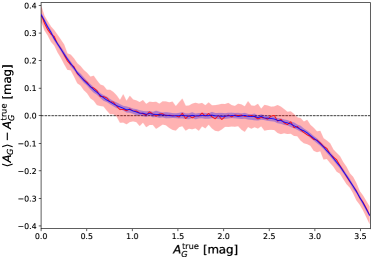
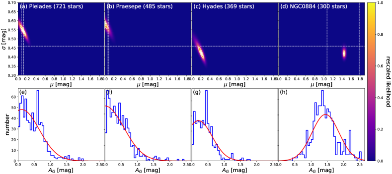
Since the sample mean is no longer a useful estimator in general, we must use the likelihood from equation 19 in order to estimate parameters. We find the maximum of the likelihood (Bayesians may add priors).222222The maximum likelihood estimate can be negative, but we truncate this to zero on the grounds that true cluster extinctions cannot be negative (this is just a prior). Highly extinct clusters could have true mag, in which case the mode may lie outside our parameter range and would be an underestimate. In Table 9 we provide our estimates for the 46 clusters from Gaia Collaboration et al. (2018a). Fig. 39 shows the likelihood function over and for the Pleiades, Praesepe, Hyades and NGC884. For Praesepe and the Pleiades, the estimated cluster extinctions agree very well with the literature values. Emphasizing the point from Fig. 38, the sample mean extinction for Praesepe is mag, whereas the maximum likelihood estimate is actually mag (see Table 9), which compares favourably with the literature estimate of 0.03 mag used in section 6.7. For the Pleiades, the sample mean is 0.48 mag while the maximum likelihood estimate is 0.11 mag (cf. literature estimate of 0.12 mag). We obtain mag and 0.54 mag for Praesepe and Pleiades respectively, which are larger than our global uncertainty estimate of 0.46 mag from section 6.5. In the case of the Hyades we clearly overestimate the cluster extinction with mag while mag is slightly below our global uncertainty estimate. (Note from Fig. 39 that these two quantities are negatively correlated when approaching the lower boundary.) We suspect this to be shot noise from the finite number of cluster members with measurements. Indeed, simulating 100 Hyades-like samples, each with true mag, true mag, and 369 stars, we observe poor estimates in 8% of the cases. It may come as a surprise that 369 stars is not necessarily sufficient to reliably estimate the cluster extinction and the scatter. The explanation is that for a low-extinction cluster such as the Hyades, the truncation of the Gaussian is dominant. We are trying to infer a pathological distribution, so the estimate of the mode of the distribution, , is more sensitive to the set of samples than is the sample mean. As an example of a cluster with higher extinction, the maximum-likelihood estimate of NGC884 (panels d and h of Fig. 39) also agrees reasonably well with the literature ( mag from Pandey et al. 2003, which corresponds to mag). Nevertheless, although our maximum-likelihood estimates of the cluster extinctions are largely consistent with the expected values, the random errors are still far too large for detailed studies of Hertzsprung-Russell diagrams in clusters.
| no. of | ML estimates | |||
|---|---|---|---|---|
| name | stars | |||
| mag | mag | mag | ||
| NGC3532 | 1217 | 0.293 | ||
| NGC2437 | 962 | 0.538 | ||
| NGC2516 | 894 | 0.373 | ||
| NGC2682 | 724 | 0.371 | ||
| Pleiades | 721 | 0.478 | ||
| NGC2168 | 709 | 0.629 | ||
| NGC6475 | 612 | 0.373 | ||
| Praesepe | 485 | 0.464 | ||
| IC4651 | 474 | 0.506 | ||
| NGC0188 | 450 | 0.585 | ||
| NGC2360 | 421 | 0.444 | ||
| Stock2 | 410 | 0.802 | ||
| NGC2447 | 377 | 0.267 | ||
| Hyades | 369 | 0.424 | ||
| NGC2422 | 343 | 0.358 | ||
| NGC6281 | 309 | 0.546 | ||
| NGC0884 | 300 | 1.445 | ||
| IC4756 | 299 | 0.597 | ||
| NGC1039 | 296 | 0.400 | ||
| alphaPer | 284 | 0.736 | ||
| NGC2548 | 284 | 0.331 | ||
| NGC6405 | 275 | 0.688 | ||
| NGC0869 | 264 | 1.423 | ||
| IC4725 | 258 | 1.088 | ||
| NGC2423 | 255 | 0.474 | ||
| NGC6025 | 243 | 0.558 | ||
| Blanco1 | 191 | 0.265 | ||
| NGC6633 | 190 | 0.562 | ||
| Trumpler10 | 175 | 0.428 | ||
| NGC7092 | 174 | 0.338 | ||
| IC2602 | 173 | 0.805 | ||
| NGC2451 | 145 | 0.747 | ||
| NGC2323 | 143 | 0.637 | ||
| NGC0752 | 141 | 0.408 | ||
| IC2391 | 134 | 0.732 | ||
| Trumpler02 | 134 | 0.848 | ||
| NGC2158 | 132 | 1.107 | ||
| NGC6774 | 127 | 0.495 | ||
| NGC2547 | 122 | 0.729 | ||
| ComaBer | 109 | 0.257 | ||
| NGC6793 | 103 | 0.962 | ||
| NGC1901 | 71 | 0.407 | ||
| NGC2232 | 70 | 0.681 | ||
| Coll140 | 63 | 0.647 | ||
| NGC3228 | 60 | 0.469 | ||
| IC4665 | 56 | 0.691 | ||
Finally, we can see from Table 9 that the maximum-likelihood estimates of vary quite considerably, sometimes being below and sometimes above our global uncertainty estimate of 0.46 mag from section 6.5. Unsurprisingly, the estimation of cluster extinctions works better for some samples than for others.