Towards Incremental
Cylindrical Algebraic Decomposition

Abstract

Cylindrical Algebraic Decomposition (CAD) is an important tool within computational real algebraic geometry, capable of solving many problems to do with polynomial systems over the reals, but known to have worst-case computational complexity doubly exponential in the number of variables. It has long been studied by the Symbolic Computation community and is implemented in a variety of computer algebra systems, however, it has also found recent interest in the Satisfiability Checking community for use with SMT-solvers. The SC² Project seeks to build bridges between these communities.

The present report describes progress made during a Research Internship in Summer 2017 funded by the EU H2020 SC² CSA. We describe a proof of concept implementation of an Incremental CAD algorithm in Maple, where CADs are built and refined incrementally by polynomial constraints, in contrast to the usual approach of a single computation from a single input. This advance would make CAD of use to SMT-solvers who search for solutions by constantly reformulating logical formula and querying solvers like CAD for whether a logical solution is admissible. We describe experiments for the proof of concept, which clearly display the computational advantages when compared to iterated re-computation.

In addition, the project implemented this work under the recently verified Lazard projection scheme (with corresponding Lazard evaluation). That is the minimal complete CAD method in theory, and this is the first documented implementation.

1 Introduction

The aim of this project is to adapt the main Cylindrical Algebraic Decomposition (CAD) algorithm for use with SMT-solvers, as part of the SC² Project which seeks to build collaborations between researchers in Symbolic Computation and Satisfiability Solving [1]. The work is influenced by the success of SAT/SMT solvers while conducting Conflict-Driven Clause Learning (CDCL) search based algorithms (see for example [2]), and their recent application to the domain of non-linear real arithmetic where CAD provides the only complete theory.

The main contributions of this report are the description of algorithms for adapting a CAD to changes in the input it is built with respect to: either incrementing or reducing the polynomial system by one constraint. We also describe results for a proof of concept implementation in the computer algebra system Maple. This shows promising experiment results with savings of up to half the calculation time, compared to a full CAD recalculation.

Other contributions are on the application side of Symbolic Computation including: an implementation of the Lazard projection and evaluation. The Lazard projection operator was proposed in 1994 [5], but shortly after a flaw was found in its proof of correctness (see [7] for details). However, recent work [8] has given an alternative proof (which necessitates changes to the lifting stage) renders this the most efficient complete CAD projection operator.

1.1 Terminology

First, we will introduce some of the basic definitions needed to follow this article. We follow the presentation in the lecture notes by Jirstrand, [4]. We work over $n$-dimension real space $\mathbb{R}^{n}$ in which there is a variable ordering $x_{1}\prec x_{2}\prec\dots\prec x_{n}$.

Definition 1 A decomposition of the space $\mathcal{X}\subset\mathbb{R}^{n}$ is a finite collection of disjoint regions (components) whose union is $\mathcal{X}$.

Definition 2 A set is semi-algebraic if it can be constructed by finitely many applications of $union$, $intersection$ and $complementation$ operations on sets of the form $\{x\in\mathbb{R}^{n}\ |\ \mathbf{f}(x)\geq 0\}$ where $\mathbf{f}\in\mathbb{R}[x_{1},\cdots,x_{n}]$.

Definition 3 A decomposition $\mathcal{D}$ is algebraic if each of its components $x\in\mathcal{D}$ is a semi-algebraic set.

Definition 4 A finite partition of $\mathcal{D}$ of $\mathbb{R}^{n}$ is called a cylindrical decomposition of $\mathbb{R}^{n}$ if the projections of any two cells onto any lower dimensional coordinate space with respect to the variable ordering are either equal or disjoint.

Note: any cylindrical decomposition of $\mathbb{R}^{n}$ implies additional cylindrical decompositions of $\mathbb{R}^{n-1},\ldots,\mathbb{R}^{1}$.

Definition 5 If a cylindrical decomposition is also an algebraic decomposition, then it is a cylindrical algebraic decomposition (CAD).

Definition 6 A CAD is traditionally produced sign-invariant with respect to a set of input polynomials, which means that each polynomial has constant sign (positive, negative or zero) on each cell.

Definition 7 The elements of a CAD are refereed to as cells. Traditionally, each cell is equipped with: a cell index which is a list of integers which defines the position of a cell in the decomposition (first index refers to $x_{1}$ etc.); and a sample point of the cell. The cells we produce also come with a cell description: a cylindrical formula.

For example, in a CAD $\mathcal{C}\in\mathbb{R}^{2}[x,y]$, a cell could be defined by the triple $[[1,1],[x<1,y<1],[0,0]]$ where: the first element $([1,1])$ specifies the index of the cell (identifying it as the least with respect to both dimensions); the second element $([x<1,y<1])$ gives the exact description of the cell; and finally the third element $([0,0])$ specifies a sample point within the cell.

1.2 Example

We give a visual example inspired by http://planning.cs.uiuc.edu/node296.html. We first take a gingerbread face and remove the detail to leave an image resembling Figure 2. This is formed by four closed curves, each of which will be defined by a bi-variate polynomial equation.

Figure 1: Closed curve reduction

Figure 2: A CAD of Fig 2.

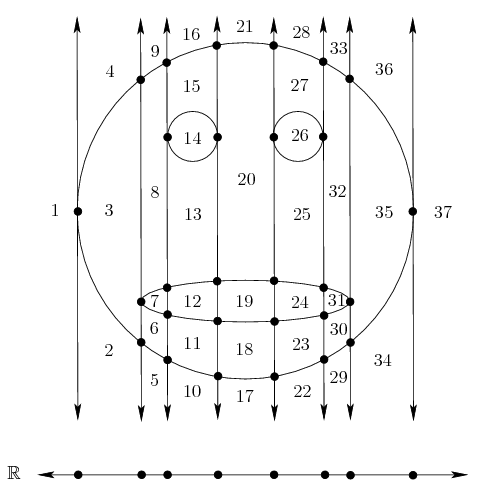
A CAD on this system of polynomials is visualised in Figure 2. Notice there are $37$ open cells (those of two dimensions). There are a further $28$ partially open (1-dimensional line segments) and $28$ closed cells (isolated points) giving $93$ CAD cells in total.

It is worth noting that in many industrial applications (especially those from SMT applications), the polynomial systems will not form aesthetically pleasing geometric shapes, and will often better resemble randomly generated systems.

1.3 New objects of study

We now formally define the two main objects of study in this report.

Definition 8 An InCAD of the space $\mathbb{R}^{n}$ is an incremental cylindrical algebraic decomposition, caused by adding a polynomial $f_{new}$ into a polynomial system $\{f_{1},\dots,f_{m}\}\in\mathbb{R}[x_{1},\dots,x_{2}]$, for which there was already has a CAD computed, producing a new CAD of $\{f_{1},\dots,f_{m},f_{new}\}\in\mathbb{R}[x_{1},\dots,x_{n}]$.

Definition 9 A ReCAD of the space $\mathbb{R}^{n}$ is a reduced cylindrical algebraic decomposition, caused by removing a polynomial $f_{m}$ from $\{f_{1},\dots,f_{m}\}\in\mathbb{R}[x_{1}\,\dots,x_{n}]$, which already has the CAD computed, producing a new CAD of $\{f_{1},..f_{m-1}\}\in\mathbb{R}[x_{1},\dots,x_{n}]$.

1.4 Report plan

The report proceeds as follows. In Section 2 we describe Lazard’s Projection scheme and in Section 3 the development and results of an incremental projection algorithm built upon this. Then in Section 4, we describe the lifting stage necessitated by Lazard projection and in Section 5 the development and results of an incremental lifting algorithm via the Lazard evaluation. We finish in Section 6 with a summary of possibilities for future work.

2 Projection

2.1 Lazard projection

The present project built upon code from the open source ProjectionCAD package [3] for Maple. This implemented the McCallum family of projection operators following [6] and needed to be adapted for the Lazard projection scheme.

First, we will introduce some notation. When we speak of projection, we usually refer to the maximal chain of projections. I.e. if a single projection eliminates one variable

$$\pi_{n-1}\mathrel{\mathop{\mathchar 58\relax}}\mathbb{R}^{n}\rightarrow\mathbb{R}^{n-1}\mathrel{\mathop{\mathchar 58\relax}}(x_{n},\ldots,x_{1})\mapsto(x_{n-1},\ldots,x_{1})$$

then we may consider chaining these with the maximal chain one less than the total number of variables

$$\pi^{*}\mathrel{\mathop{\mathchar 58\relax}}\mathbb{R}^{n}\rightarrow\mathbb{R}^{1}\mathrel{\mathop{\mathchar 58\relax}}(x_{n},\ldots,x_{1})\mapsto(x_{1}).$$

In this article we will refer to the Lazard projection operator [5], [8] as ProjL and the McCallum projection operator ProjM [6].

Algorithm 1 shown later performs the Lazard projection. It is almost identical to the counterpart McCallum projection function in the ProjectionCAD package. Both take all the discriminants and cross resultants of the input polynomials. The differences arise when taking coefficients from a polynomial in the sub-function Algorithm 2. Lazard takes only the leading and trailing coefficients as opposed to all coefficients. Hence $\textit{ProjL}(\mathcal{F})\subset\textit{ProjM}(\mathcal{F})$. Algorithm 1 iterates to perform the maximum chain or projections and produce the full set of projection polynomials.

We will assume familiarity with the details of projection and lifting for CAD, so that we can focus more on the new contributions. Further details can be found in [4] or [3] for the implementation at hand.

Notation We use wrt in place of with respect to.

Definition 10 Set n_elements($Polys$) to be the number of elements in the set of polynomials $Polys$.

Definition 11 Set degree$(F,x)$ to be the degree of the polynomial $F$, wrt to variable x.

Definition 12 Set RR$(x)$ to be the function which returns a set of unique real roots of polynomial x.

Definition 13 Set R$(x)$ to be the function which reduces polynomial x to its square free unique factors, with constant multiples removed.

Notation The three core algorithms implemented for the classical Lazard projection were: ProjectionPolys, Projection and CoefficientSet.
ProjectionPolys is effectively $\pi^{*}$, Projection is $\pi_{n_{2}}$, where $n_{2}$ is a parameter specified in the input and CoefficientSet which collects the coefficients required for the $n_{2}$’th Lazard projection.

2.2 Worked example

Before introducing the reader to the generalised algorithm, we will first go through, step by step, a bi-variate case of projection. We will later use this example to build upon for the incremental instance. We begin by calculating the projection from the following polynomial system (1):

$$\textbf{F}_{1}=\{\underbrace{x_{1}^{2}+x_{2}^{2}-1}_{f_{1}},\underbrace{x_{1}^{3}-x_{2}^{2}}_{f_{2}}\}.$$ (1)

Here, the first polynomial is denoted $f_{1}$ and second denoted $f_{2}$. We first go through and calculate the univariate polynomials produced by projection and the corresponding real roots. Later, we will use this projection set to lift and build a CAD. We have left out the explicit output polynomials to save space but they can be easily calculated by most computer algebra systems.

$$\begin{array}[]{ll}r1=\texttt{Resultant}(f_{1},f_{2},x_{2}),&\texttt{RR}(r1)=\{\alpha_{1}\}\approx\{0.7549\}\\ d1=\texttt{Discriminant}(f_{1},x_{2}),&\texttt{RR}(d1)=\{0\}\\ d2=\texttt{Discriminant}(f_{2},x_{2}),&\texttt{RR}(d2)=\{-1,1\}\\ l1=\texttt{Leading\ Coefficient}(f_{1},x_{2}),&\texttt{RR}(l1)=\{\}\\ l2=\texttt{Leading\ Coefficient}(f_{2},x_{2}),&\texttt{RR}(l2)=\{\}\\ t1=\texttt{Trailing\ Coefficient}(f_{2},x_{2}),&\texttt{RR}(t1)=\{-1,1\}\\ t2=\texttt{Trailing\ Coefficient}(f_{2},x_{2}),&\texttt{RR}(t2)=\{0\}\\ \end{array}$$ (2)

So the complete set of isolated real roots is the union: $\{-1,0,\alpha_{1}\approx 0.7549,1\}\\$

In the presentation above we assigned an irrational root to a symbol and gave a decimal approximation, but the implementation would contain the exact root as an algebraic number.

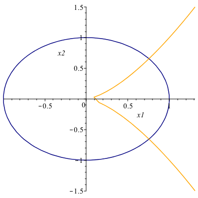
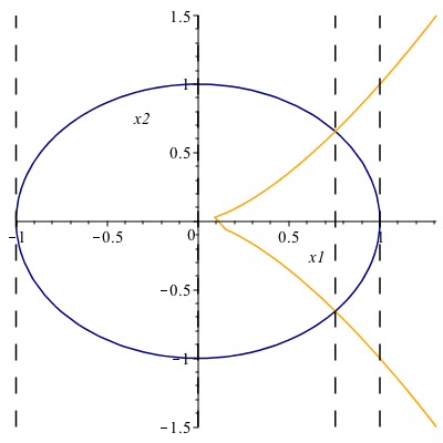
Figures 3 and 4 plots the graphs of these functions along with the real roots isolated. We see they correspond to geometrically relevant features.

Figure 3: The blue curve is $f_{1}$ and the orange curve is $f_{2}$.

Figure 4: Dotted lines show the projection roots.

2.3 Incremental Lazard projection

The most appealing approach for creating InCAD was to adapt the Lazard Projection algorithms only to calculate the new projection polynomials. To do this Algorithm 1 and Algorithm 2 had to be modified.The aim was to directly take the output from the previous call of Projection, together with the incremental polynomial and receive the incremented projection set. We outline the four required adjustments below, how we implemented these adjustments, as well as indicate their active state within the algorithm by highlighting the changes to the algorithms in blue in Algorithms 3 and 4 (ProjectionAdd and ProjectionPolysAdd).

ProjectionPolysAdd is effectively $\pi^{*}$ for the incremental case, ProjectionAdd is $\pi_{n_{2}}$, where $n_{2}$ is a parameter specified in the input. Note that CoefficientSet itself was unchanged, only the argument passed to it was different. The new argument is now polynomials exclusively from the new polynomial set.

2.3.1 Worked example

In a similar fashion to Section $2.2$, we will guide the reader through a basic incremental example. We will start by incrementing the polynomial system $\textbf{F}_{1}$, with the polynomial forming a linear line, $f_{3}=x_{2}-x_{1}$. This forms the new system (3).

$$\textbf{F}_{2}=\{\underbrace{x_{1}^{2}+x_{2}^{2}-1,x_{1}^{3}-x_{2}^{2}}_{\textbf{F}_{1}},\underbrace{x_{2}-x_{1}}_{f_{3}}\}$$ (3)

The additional projection polynomials and their real roots are:

$$\begin{array}[]{ll}r2=\texttt{Resultant}(f_{1},f_{3},x_{2}),&\texttt{RR}(r2)=\{\pm\alpha_{2}=\pm\frac{1}{\sqrt[]{2}}\approx\pm 0.7071\}\\ r3=\texttt{Resultant}(f_{2},f_{3},x_{2}),&\texttt{RR}(r3)=\{-1,0\}\\ d3=\texttt{Discriminant}(f_{3},x_{2}),&\texttt{RR}(d3)=\{\}\\ l3=\texttt{Leading\ Coefficient}(f_{3},x_{2}),&\texttt{RR}(l3)=\{\}\\ t3=\texttt{Trailing\ Coefficient}(f_{3},x_{2}),&\texttt{RR}(t3)=\{0\}\\ \end{array}$$ (4)

So we have rediscovered two roots seen before ($0$ and $-1$) and two new ones ($\pm\alpha_{2}$). The total ordered set of real roots is now

$$\{-1,-\alpha_{2}\approx-0.7071,0,\alpha_{2}\approx 0.7071,\alpha_{1}\approx 0.7549,1\}\\$$

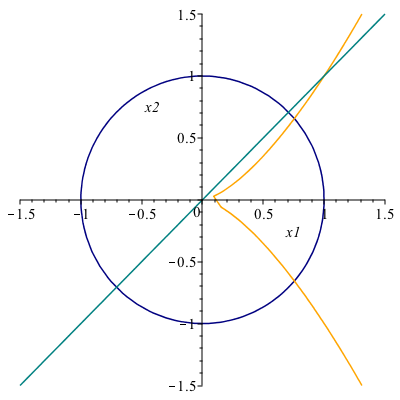
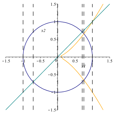
Figures 5 and 6 show that the two new roots correspond to the two new intersections of the straight line with the circle. The other new intersections happened to coincide with other already identified features.

Figure 5: The blue curve is $f_{1}$, the orange $f_{2}$ and the teal curve $f_{3}$.

Figure 6: Dotted lines show the projection roots $\in\mathcal{R}$.

2.3.2 Algorithms

The adjustments required to transfer to an incremental Lazard projection system are detailed as follows:

1. To output the full table of projection polynomials organised by the main variable and reinput this with incremental calls. This output would then be used as an input for ProjectionPolysAdd.

2. The process and pass the new polynomials into ProjectionAdd.

3. To create a storage system of new polynomials which we could then apply the minimal number of operations required to obtain the correct Psetnew[i], for each index of i. We introduced a new table called Pset[3] storing the new polynomials created at each iteration of Algorithm 1.

2.4 Incremental projection results

Notice there were seven elements of the projection set to calculate in the original projection system ProjL($F_{1}$). If we were to recompute the incremental system ProjL($F_{2})$ using the standard method, we would have to compute twelve elements of the projection (the original 7 plus 5 more). This would be more than double the workload of computing just those 5.

We split the testing into two experiments, one where we tested the projection algorithm on a test set of 80 examples, the other of 60 more straightforward cases. The first test set is of 80 pairs of tri-variate polynomial couples, each with four terms. The second test set contained 60 pairs of bi-variate polynomials, each with three variates. A pair consists of polynomial a and polynomial b, where b is the polynomial added incrementally. These pairs were created using the random polynomial generating function in Maple. The testing code is openly available.

An example from the tri-variate, four-term test (with chosen variable ordering $[z,y,x]$):

$$[-79x^{2}y^{3}+97y^{2}z^{2}+51x^{2},71x^{3}y^{2}+22xz-47y^{2}]$$ (5)

An example from the bi-variate, three-term test (with variable ordering $[z,y]$):

$$[66z^{5}-40y^{4}+75yz^{2}+83z,-33y^{2}z^{3}+72y^{3}z+84yz^{2}-4z^{2}]$$ (6)

The tests were controlled by a bash script rather than code within a single Maple session to avoid any caching which could bias the results.

2.4.1 Experiment: Tri-variate

When looking at the cases which were faster, they were on average faster by $30\%$, and $39\%$ slower in the other cases. The net speed difference had a mean of $28\%$ increase in performance with the incremental projection.

Projection	Results
	Classical	Incremental
Variance	0.002743s	0.002205s	24.39% Smaller
Mean	0.06739s	0.04809s	28.64% Faster
Lower Quartile	0.02475s	0.013s	47.47% Faster
Median	0.0625s	0.035s	44.00% Faster
Upper Quartile	0.09425s	0.07525s	20.16% Faster

2.4.2 Experiment: Bi-variate

When looking at the cases which were faster, they were on average faster by $55\%$, and $87\%$ slower in the other cases. The net speed difference had a mean of $16\%$ increase in performance with the incremental projection.

Projection	Results
	Classical	Incremental
Variance	0.0004660s	0.0006425s	27.46% Larger
Mean	0.03743s	0.0315s	15.85% Faster
Lower Quartile	0.024s	0.008s	66.66% Faster
Median	0.0285s	0.015s	47.39% Faster
Upper Quartile	0.03675s	0.05525s	50.34% Slower

Algorithm 1 ProjectionPolys

1:  Input: A system of polynomials $polyset=\{f_{1},\ldots,f_{m}\}\in\mathbb{R}[x_{n},\ldots,x_{1}]$, $var=[x_{n},\ldots,x_{1}]$

2:  Output: A list of projection polynomials $\in\mathbb{R}[x_{n-1},\dots,x_{1}]$

3:  Procedure Lazard ProjectionPolys {”Compute the full chain of projections”}

4:  $dim\leftarrow$ Number of elements in $var$

5:  $pset[0]=table()$

6:  $pset[0]\leftarrow$ Primitive set from $polyset$, wrt variable $x_{n}$

7:  $pset[0]\leftarrow$ Square free basis set from $pset[0]$, wrt variable $x_{n}$

8:  $pset[0]\leftarrow$ Set of factors from $pset[0]$, wrt variable $x_{n}$

9:  $cont\leftarrow$ Content Set from $polyset$, wrt variable $x_{n}$

10:  for i from 1 to dim-1 do

11:     $out\leftarrow$ Projection$(pset[i-1],x_{n-i+1},[x_{n-i},\ldots,x_{1}])$

12:     $pset[i]\leftarrow(out\ \cup\ cont)$

13:     $cont\leftarrow$ Content set from $pset[i]$, wrt $x_{n-i}$

14:     $pset[i]\leftarrow$ Primitive set from $pset[i]$, wrt variable $x_{n-i}$

15:     $pset[i]\leftarrow$ Square free basis set from $pset[i]$, wrt variable $x_{n-i}$

16:     $pset[i]\leftarrow$ Set factors from $pset[i]$, wrt variable $x_{n-i}$

17:  end for

18:  $ret\leftarrow pset[dim-1]$

19:  $ret\leftarrow$ Remove constant multiples from $ret$

20:  return $ret$

Algorithm 2 Projection

1:  Input: A set of polynomials $polyset=\{f_{1},\ldots,f_{m}\}\in\mathbb{R}[x_{n},\ldots,x_{1}]$, $var=x_{n}$ and $lvars=[x_{n-1},\ldots,x_{1}]$

2:  Output: A set of projection polynomials $\mathbb{P}=\{p_{1},\ldots,p_{q}\}\in\mathbb{R}[x_{n-1},\ldots,x_{1}]$

3:  Procedure Lazard Projection {”Lazard projection operator, $\pi_{n-1}$.”}

4:  $Polys\leftarrow$ Primitive set from $polyset$, wrt variable $x_{n}$

5:  $Cont\leftarrow$ Content set from $polyset$, wrt variable $x_{n}$

6:  $Polys\leftarrow$ Square free basis from $Polys$, wrt $x_{n}$

7:  $Pset1=table()$

8:  for i from 1 to n_elements(Polys) do

9:     $Pol\leftarrow Polys[i]$

10:     $clist\leftarrow$ Lazard coefficient set from $Pol$, wrt variable $x_{n}$

11:     $temp\leftarrow$ Discriminant set from $Pol$, wrt variable $x_{n}$

12:     $temp\leftarrow$ Remove constant multiples from $temp$

13:     $Pset1[i]\leftarrow$ Concatenate together $temp$ and $clist$ {Need to make sure you deal with the case of temp being empty here}

14:  end for

15:  $Pset2=table()$

16:  for i from 1 to n_elements(Polys) do

17:     for j from i+1 to n_elements(Polys) do

18:        $Pset2[i,j]\leftarrow$ Resultant of the two polynomials $Polys[i]$ & $Polys[j]$, wrt variable $var$

19:        $Pset2[i,j]\leftarrow$ Remove constant multiples from $Pset2[i,j]$

20:     end for

21:  end for

22:  $Pset\leftarrow cont,Pset1,Pset2$ {Note that $Pset\in\mathbb{R}[x_{n-1},\ldots,x_{1}]$}

23:  $Pset\leftarrow$ Remove constants from $Pset$

24:  return $Pset$

Algorithm 3 ProjectionPolysAdd

1:  Input: A system of polynomials $polyset=\{f_{1},..f_{m}\}\in\mathbb{R}[x_{n},..,x_{1}]$, $prevprojset\in\mathbb{R}[x_{n},\ldots,x_{1}]$, $newpolset\in\mathbb{R}[x_{n},\ldots,x_{1}]$ and $vars=[x_{n},..,x_{1}]$ (Adjustment 1)

2:  Output: A list of projection polynomials $\in\mathbb{R}[x_{n-1},..,x_{1}]$

3:  Procedure Lazard ProjectionPolysAdd {”Compute the full chain of projections, $\pi*$”}

4:  $dim\leftarrow$ Number of elements in $vars$ $+1$

5:  $pset[0]=table()$

6:  $pset[0]\leftarrow$ Primitive set from $newpolset$, wrt variable $x_{n}$ (Adjustment 2)

7:  $pset[0]\leftarrow$ Square free basis set from $pset[0]$, wrt variable $x_{n}$

8:  $pset[0]\leftarrow$ Set of factors from $pset[0]$, wrt variable $x_{n}$

9:  $cont\leftarrow$ Set of contents of $newpolset$, wrt $x_{n}$ (Adjustment 2)

10:  for i from 1 to dim-1 do

11:     $out\leftarrow$ ProjectionAdd$({\color[rgb]{0,0,1}prevprojset[i-1]},pset[i-1],x_{n-i+1},\ldots,x_{1})$ (Adjustment 2)

12:     $pset[i]\leftarrow(out\ \cup\ cont)$

13:     $cont\leftarrow$ Content set from $pset[i]$, wrt variable x_n-i

14:     $pset[i]\leftarrow$ Prime set from $pset[i]$, wrt variable $x_{n-i}$

15:     $pset[i]\leftarrow$ Square free basis from set $pset[i]$, wrt variable $x_{n-i}$

16:     $pset[i]\leftarrow$ Set factors from $pset[i]$, wrt variable $x_{n-i}$

17:  end for

18:  $pset[dim-1]\leftarrow$ Remove constant multiples from $pset[[dim-1]$

19:  $ret\leftarrow pset[[dim-1]$

20:  return $pset$ (Adjustment 1)

Algorithm 4 ProjectionAdd

1:  Input: Polynomial set $newpprojset=\{f_{1},..f_{m}\}\in\mathbb{R}[x_{n},\ldots,x_{1}]$, $oldprojset\in\mathbb{R}[x_{n-1},\ldots,x_{1}]$, and variable ordering (Adjustment 2)

2:  Output: Set of polynomials $Pset=\{p_{1},\ldots,p_{q}\}\in\mathbb{R}[x_{n-1},\ldots,x_{1}]$

3:  Procedure Lazard ProjectionAdd {The incremental version of the Lazard projection operator, $\pi_{n-1}$.}

4:  $Polys\leftarrow$ Primitive set from $newpprojset$, wrt variable $x_{n}$ (Adjustment 2)

5:  $Cont\leftarrow$ Content set from $newpprojset$, wrt variable $x_{n}$ (Adjustment 2)

6:  $Polys\leftarrow$ Square free basis set from $Polys$, wrt variable $x_{n}$

7:  $Pset1=table()\mathrel{\mathop{\mathchar 58\relax}}$

8:  for i from 1 to number_elements(Polys) do

9:     $Pol\leftarrow Polys[i]$

10:     $clist\leftarrow$ Lazard coefficient set from $Pol$, wrt to $x_{n}$

11:     $temp\leftarrow$ Discriminant set from $Pol$, wrt $x_{n}$

12:     $temp\leftarrow$ Remove constant multiples from $temp$

13:     $Pset1[i]\leftarrow$ concat $temp$ & $clist$

14:  end for

15:  $Pset2=table()\mathrel{\mathop{\mathchar 58\relax}}$

16:  for i from 1 to n_elements(Polys) do

17:     for j from i+1 to n_elements(Polys) do

18:        $Pset2[i,j]\leftarrow$ Resultant of $Polys[i]$ and $Polys[j]$, wrt to variable $var$

19:        $Pset2[i,j]\leftarrow$ Remove constant multiples from $Pset2[i,j]$

20:     end for

21:  end for

22:  $oldset\leftarrow oldprojset$

23:  $Pset3=table()\mathrel{\mathop{\mathchar 58\relax}}$

24:  for i from 1 to n_elements(Polys) do

25:     for j from 1 to n_elements(oldset) do

26:        $Pset3[i,j]\leftarrow$ Resultant of $Polys[i]$ and $oldset[j]$, wrt to variable $var$

27:        $Pset3[i,j]\leftarrow$ Remove constant multiples from $Pset3[i,j]$

28:     end for

29:  end for{Adjustment 3}

30:  $Pset\leftarrow$ concat $(cont,Pset1,Pset2,{\color[rgb]{0,0,1}Pset3})$ {$Pset\in\mathbb{R}[x_{n},\ldots,x_{1}]$}

31:  $Pset\leftarrow$ Remove constant multiples from $Pset$

32:  return $Pset$

3 Lifting

3.1 Lifting after Lazard projection

We had to make changes to the lifting code not just to allow for incrementality but also changes required by the use of Lazard projection as set out in [8]. This requires the use of Lazard evaluation of polynomials (Algorithm 5). To simplify we restricted our implementation to the open case.

Definition 14 An Open-CAD is one produced by lifting over open intervals only. Thus it is not a full decomposition of ${\mathbb{R}}^{n}$ as the boundaries of the full dimensional cells are missing.

The advantage is that when building an Open-CAD we need never extend over irrational sample points, avoiding costly algebraic number calculations, but still getting a good understanding of the solution set.

We will now discuss a method used for incremental lifting, which can be thought of graphically, as a form of acyclic tree merge, later displayed visually. It will first make more sense if we explicitly show the reader the mathematical structure that allows CAD to be represented as a tree. Keeping the structure shown here in mind, will in hope make most of the algorithmic decisions, implemented during incremental lifting, much clearer.

We have two core algorithms for the Lifting. First the initial LiftSetup set-up algorithm (Algorithm 6), and then Lift (Algorithm 7) which iterates over the variable ordering until completion. There are also a number of other less complicated vital sub algorithms used for cell formatting/sorting/lifting purposes such NewCadCells, which creates new cells when lifting to a set of given roots, GenSamplePoints for generating sample points, SubsFormat which formats the sample points for substitution.

3.2 Worked example and Lazard evaluation

Definition 15 Let divide$(x,d)$ to be the function returns boolean value true if $x$ is divisible by polynomial $d$, otherwise false.

Definition 16 Let SDivide$(x,d,v)$ to be the function will completely divide polynomial $d$; which is for example $\in\mathcal{R}[x_{1}]$, out of polynomial $x\in\mathcal{R}[x_{1},x_{2}]$, until the output is no longer divisible by $d$. in which case SDivide will then take this polynomial and substitutes the value $v$ into all instances of the variable $x_{1}$, returning a square free univariate polynomial in $x_{2}$.

We will guide the reader through a primary Lazard lift example, using Lazard evaluation (Algorithm 5). The key difference to traditional CAD lifting is that we must calculate the Lazard evaluation of each polynomial at each sample point. This avoids the well-orientedness issues of the McCallum projection operators (where information is lost due to nullification at a point).

Algorithm 5 Lazard evaluation

1:  Input: A polynomial from the projection set $f\in\mathbb{R}[x_{1},\ldots,x_{d}]$, and $\texttt{samplepoints}=[r_{1},\ldots,r_{d-1}]\in\mathbb{R}^{d-1}$.

2:  Output: List of roots.

3:  Procedure Lazard_evaluation:

4:  Set roots to be an empty list

5:  for $j$ from $1$ to $d-1$ do

6:     Break if cell is zero dimensional.

7:     for $i$ from $1$ to degree$(f,x_{j})$ do

8:        if f is divisible by $x_{j}-r_{j}$ then

9:           $f\leftarrow f/(x_{j}-r_{j})$

10:        else

11:           break innermost for loop:

12:        end if

13:     end for

14:  end for

15:  $f\leftarrow$ Substitute the samplepoints into $f$

16:  {$f\in\mathbb{R}[x_{n},\ldots,x_{d}]$}

17:  $roots\leftarrow$ Real roots of $f$

18:  $roots\leftarrow$ Remove duplicates and sort $roots$ in ascending order

19:  return roots:

We will start by lifting the projection polynomial system defined previously ProjL($\textbf{F}_{1}$), described below. In our implementation, we only performed the lift over open intervals, as we followed the Open-CAD method. However, for this example, we will lift all cells.

$$\texttt{ProjL}(\textbf{F}_{1})=\{x_{1}+1,x_{1},x_{1}-\alpha_{1},x_{1}-1\}$$ (7)

First, we must generate our sample points for the decomposition of the real line with respect to the roots $\{-1,0,\alpha_{1},1\}$. Thus, we need a sample value from each of the following cells:

$$\begin{array}[]{lll}a1=\{x_{1}<-1\},&a2=\{x_{1}=-1\},&a3=\{-1<x_{1}<0\},\\ a4=\{x_{1}=0\},&a5=\{0<x_{1}<\alpha_{1}\},&a6=\{x_{1}=\alpha_{1}\},\\ a7=\{\alpha_{1}<x_{1}<1\},&a8=\{x_{1}=1\},&a9=\{1<x_{1}\}\end{array}$$ (8)

Note: $ai$ denotes the sorted $i$’th cell in the decomposition of $x_{1}$-space.

Our nine chosen sample points are:

$$\begin{array}[]{l}\texttt{SamplePoints}(\texttt{ProjL}(\textbf{F}_{1}))=\{-2,-1,-0.5,0,0.5,\alpha_{1}\approx 0.7549,0.9,1,2\}\\ \end{array}$$ (9)

Now we lift over each cell at the designated sample point by isolating real roots of the corresponding univariate polynomials. Below, $p_{i,j}$ denotes the polynomial acquired after applying the Lazard evaluation method to the $i$’th sample point, on the $j$’th polynomial from $F_{1}$

$$\begin{array}[]{l}\textnormal{Performing lift on the first sample point of }$$-2\mathrel{\mathop{\mathchar 58\relax}}$$\\ p_{1,1}=\texttt{SDivide}(f_{1},(x_{1}+2),-2),\ \ \ \texttt{RR}(p_{1,1})=\{\}\\ p_{1,2}=\texttt{SDivide}(f_{2},(x_{1}+2),-2),\ \ \ \texttt{RR}(p_{1,2})=\{\}\\ \\ \textnormal{Performing lift on the next sample point }$$-1\mathrel{\mathop{\mathchar 58\relax}}$$\\ p_{2,1}=\texttt{SDivide}(f_{1},(x_{1}+1),-1),\ \ \ \texttt{RR}(p_{2,1})=\{0\}\\ p_{2,2}=\texttt{SDivide}(f_{2},(x_{1}+1),-1),\ \ \ \texttt{RR}(p_{2,2})=\{\}\\ \\ \textnormal{Performing lift on the next sample point }$$-0.5\mathrel{\mathop{\mathchar 58\relax}}$$\\ p_{3,1}=\texttt{SDivide}(f_{1},(x_{1}+0.5),-0.5),\ \ \ \texttt{RR}(p_{3,1})=\{-\beta_{0}\approx-0.8660,\beta_{0}\approx 0.8660\}\\ p_{3,2}=\texttt{SDivide}(f_{2},(x_{1}+0.5),-0.5),\ \ \ \texttt{RR}(p_{3,2})=\{\}\\ \\ \textnormal{Performing lift on the next sample point }$$0\mathrel{\mathop{\mathchar 58\relax}}$$\\ p_{4,1}=\texttt{SDivide}(f_{1},(x_{1}),0),\ \ \ \texttt{RR}(p_{4,1})=\{-1,1\}\\ p_{4,2}=\texttt{SDivide}(f_{2},(x_{1}),0),\ \ \ \texttt{RR}(p_{4,2})=\{\}\\ \end{array}$$

$$\begin{array}[]{l}\textnormal{Performing lift on the next sample point }$$0.5\mathrel{\mathop{\mathchar 58\relax}}$$\\ p_{5,1}=\texttt{SDivide}(f_{1},(x_{1}-0.5),0.5),\ \ \ \texttt{RR}(p_{5,1})=\{-\beta_{1}\approx-0.8660,\beta_{1}\approx 0.8660\}\\ p_{5,2}=\texttt{SDivide}(f_{2},(x_{1}-0.5),0.5),\ \ \ \texttt{RR}(p_{5,2})=\{-\beta_{2}\approx-0.3536,\beta_{2}\approx 0.3536\}\\ \\ \textnormal{Performing lift on the next sample point }\alpha_{1}\mathrel{\mathop{\mathchar 58\relax}}\\ p_{6,1}=\texttt{SDivide}(f_{1},(x_{1}-0.5),0.5),\ \ \ \texttt{RR}(p_{5,1})=\{-\beta_{3}\approx-0.6559,\beta_{3}\approx 0.6559\}\\ p_{6,2}=\texttt{SDivide}(f_{2},(x_{1}-0.5),0.5),\ \ \ \texttt{RR}(p_{5,2})=\{-\beta_{4}\approx-0.6559,\beta_{4}\approx 0.6559\}\\ \\ \textnormal{Performing lift on the next sample point }$$0.9\mathrel{\mathop{\mathchar 58\relax}}$$\\ p_{7,1}=\texttt{SDivide}(f_{1},(x_{1}-0.9),0.9),\ \ \ \texttt{RR}(p_{7,1})=\{-\beta_{5}\approx-0.4359,\beta_{5}\approx 0.4359\}\\ p_{7,2}=\texttt{SDivide}(f_{2},(x_{1}-0.9),0.9),\ \ \ \texttt{RR}(p_{7,2})=\{-\beta_{6}\approx-0.8538,\beta_{6}\approx 0.8538\}\\ \\ \textnormal{Performing lift on the next sample point }$$1\mathrel{\mathop{\mathchar 58\relax}}$$\\ p_{8,1}=\texttt{SDivide}(f_{1},(x_{1}-1),1),\ \ \ \texttt{RR}(p_{8,1})=\{0\}\\ p_{8,2}=\texttt{SDivide}(f_{2},(x_{1}-1),1),\ \ \ \texttt{RR}(p_{8,2})=\{-1,1\}\\ \\ \textnormal{Performing lift on the next sample point }$$2\mathrel{\mathop{\mathchar 58\relax}}$$\\ p_{9,1}=\texttt{SDivide}(f_{1},(x_{1}-2),2),\ \ \ \texttt{RR}(p_{9,1})=\{\}\\ p_{9,2}=\texttt{SDivide}(f_{2},(x_{1}-2),2),\ \ \ \texttt{RR}(p_{9,2})=\{-\beta_{7}\approx-2.8284,\beta_{7}\approx 2.8284\}\end{array}$$

We now have enough information to generate our CAD cells in ${\mathbb{R}}^{2}$. To describe our full CAD system more concisely, we will now define a new set of inequalities (10) we have acquired from the lift stage into $x_{2}$. For simplicity, we will display the CAD’s created throughout this article using a graphical tree representation Fig (7). Here $bi,j$ denotes the sorted $j$’th inequality we have decomposed the $ai$’th inequality into, and so $[i,j]$ corresponds to the classical CAD cell index.

Figure 7: CAD tree of $F_{1}$. The green nodes represent cells in the first dimension and red nodes represent cells in the second dimension.

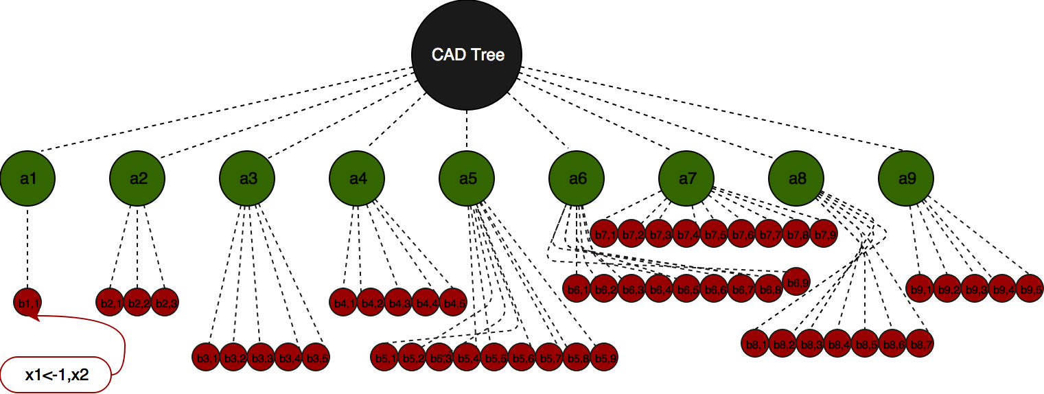
The new cell definitions are as given below.

$$\textrm{Inequalities}(\textbf{F}_{1})=$$ (10)

$$\begin{array}[]{l}b_{1,1}=\{x_{2}\},\,b_{2,1}=\{x_{2}<0\},b_{2,2}=\{x_{2}=0\},\,b_{2,3}=\{0<x_{2}\},\\ b_{3,1}=\{x_{2}<-\beta_{0}\},b_{3,2}=\{x_{2}=-\beta_{0}\},b_{3,3}=\{-\beta_{0}<x_{2}<\beta_{0}\},\\ b_{3,4}=\{x_{2}=\beta_{0}\},b_{3,5}=\{\beta_{0}<x_{2}\},\,b_{4,1}=\{x_{2}<-1\},b_{4,2}=\{x_{2}=-1\},\\ b_{4,3}=\{-1<x_{2}<1\},b_{4,4}=\{x_{2}=1\},b_{4,5}=\{1<x_{2}\},\\ b_{5,1}=\{x_{2}<-\beta_{1}\},b_{5,2}=\{x_{2}=-\beta_{1}\},b_{5,3}=\{-\beta_{1}<x_{2}<-\beta_{2}\},\\ b_{5,4}=\{x_{2}=-\beta_{2}\},b_{5,5}=\{-\beta_{2}<x_{2}<\beta_{2}\},b_{5,6}=\{x_{2}=\beta_{2}\},\\ b_{5,7}=\{\beta_{2}<x_{2}<\beta_{1}\},b_{5,8}=\{x_{2}=\beta_{1}\},b_{5,9}=\{\beta_{1}<x_{2}\},\\ b_{6,1}=\{x_{2}<-\beta_{3}\},b_{6,2}=\{x_{2}=-\beta_{3}\},b_{6,3}=\{-\beta_{3}<x_{2}<-\beta_{4}\},\\ b_{6,4}=\{x_{2}=-\beta_{4}\},b_{6,5}=\{-\beta_{4}<x_{2}<\beta_{4}\},b_{6,6}=\{x_{2}=\beta_{4}\},\\ b_{6,7}=\{\beta_{4}<x_{2}<\beta_{3}\},b_{6,8}=\{x_{2}=\beta_{3}\},b_{6,9}=\{\beta_{3}<x_{2}\},\\ b_{7,1}=\{x_{2}<-\beta_{6}\},b_{7,2}=\{x_{2}=-\beta_{6}\},b_{7,3}=\{-\beta_{6}<x_{2}<-\beta_{5}\},\\ b_{7,4}=\{x_{2}=-\beta_{5}\},b_{7,5}=\{-\beta_{5}<x_{2}<\beta_{5}\},b_{7,6}=\{x_{2}=\beta_{5}\},\\ b_{7,7}=\{\beta_{5}<x_{2}<\beta_{6}\},b_{7,8}=\{x_{2}=\beta_{6}\},b_{7,9}=\{\beta_{6}<x_{2}\},\\ b_{8,1}=\{x_{2}<-1\},b_{8,2}=\{x_{2}=-1\},b_{8,3}=\{-1<x_{2}<0\},\\ b_{8,4}=\{x_{2}=-0\},b_{8,5}=\{0<x_{2}<1\},b_{8,6}=\{x_{2}=1\},b_{8,7}=\{1<x_{2}\},\\ b_{9,1}=\{x_{2}<-\beta_{7}\},b_{9,2}=\{x_{2}=-\beta_{7}\},b_{9,3}=\{-\beta_{7}<x_{2}<\beta_{7}\},\\ b_{9,4}=\{x_{2}=\beta_{7}\},b_{9,5}=\{\beta_{7}<x_{2}\}.\end{array}$$ (28)

3.3 Incremental Lazard lifting

The two novel algorithms created for incremental lifting were the
LiftSetupAdd (Algorithm 8); the incremental version of LiftSetup (Algorithm 6), and LiftAdd (Algorithm 9); the incremental version of Lift (Algorithm 7).

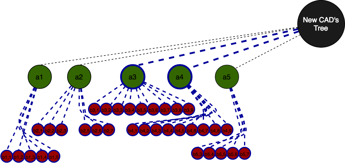
The general concept of how we solved this stage of the problem was to think of it as solving a graph (tree) attachment/detachment problem. If you think of the old CAD as having a tree structure which we save, where nodes are cells, and branches link a cell to its parent (cell it projects onto) or child (decomposition in a cylinder above) cells. At each depth of the CAD/tree, say depth $p$, are all the cells within $\mathbb{R}^{p}$ before we lifted to $\mathbb{R}^{p+1}$. We first go through a worked example before describing the general process.

We will now perform an incremental lift on the polynomial system $\textbf{F}_{1}$, incremented by a new polynomial $f_{4}=x_{1}^{3}+x_{2}^{2}$, forming the new system (29).

$$\textbf{F}_{3}=\{\underbrace{x_{1}^{2}+x_{2}^{2}-1,x_{1}^{3}-x_{2}^{2}}_{\textbf{F}_{1}},\underbrace{x_{1}^{3}+x_{2}^{2}}_{f_{4}}\}$$ (29)

The new system is symmetrical about the $y$ axis as you can see in Figure 8.

Figure 8: The blue curve is $f_{1}$, the orange $f_{2}$ and the teal $f_{4}$.

Figure 9: Dotted lines show the projection roots.

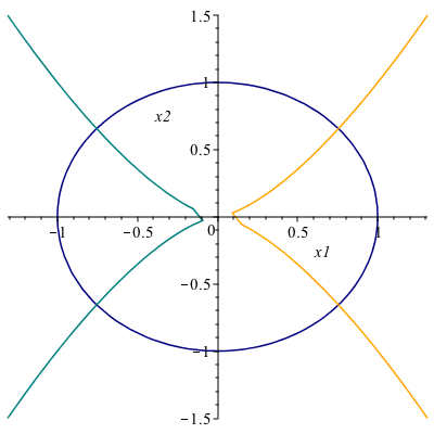
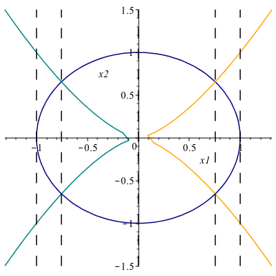
We will skip the projection steps. However they are contained in detail within the Maple ”Worked Examples” worksheet, available on GitHub.

$$\texttt{ProjL}(\textbf{F}_{3})=\ \{\underbrace{x_{1}+1}_{\texttt{ProjL}(\textbf{F}_{1})},\underbrace{x_{1}+\alpha_{1}}_{new},\underbrace{x_{1},x_{1}-\alpha_{1},x_{1}-1}_{\texttt{ProjL}(\textbf{F}_{1})}\}$$ (30)

We will be using calculations from Section 3.2 where we have already performed a full lift on the part of the system, bar the new projection polynomial of $x_{1}+\alpha_{1}$.

Incremental Lift

We now have an enlarged set of roots of univariate projection polynomials, $\{-1,-\alpha_{1},0,\alpha_{1},1\}$. The new additions below due to adding in $f_{4}$ are highlighted in blue.

Decomposition of the real line:

$$\begin{array}[]{l}a1=\{x_{1}<-1\},a2=\{x_{1}=-1\},{\color[rgb]{0,0,1}a3=\{-1<x_{1}<-\alpha_{1}\}},\\ {\color[rgb]{0,0,1}a4=\{x_{1}=-\alpha_{1}\}},{\color[rgb]{0,0,1}a5=\{-\alpha_{1}<x_{1}<0\}},a6=\{x_{1}=0\},a7=\{0<x_{1}<\alpha_{1}\},\\ a8=\{x_{1}=\alpha_{1}\},a9=\{\alpha_{1}<x_{1}<1\},a10=\{x_{1}=1\},a11=\{1<x_{1}\}\\ \end{array}$$ (31)

Corresponding sample points:

$$\begin{array}[]{l}\texttt{SamplePoints}(ProjL(\textbf{F}_{3}))=\\ \{-2,-1,{\color[rgb]{0,0,1}-0.9},{\color[rgb]{0,0,1}-\alpha_{1}},-0.5,0,0.5,\alpha_{1}\approx 0.7549,0.9,1,2\}\\ \end{array}$$ (32)

We first begin testing whether each fixed sample point has a new root, in the new projection polynomials, due to the incremental polynomial $f_{4}$. If it does, we will merge the new roots into the old roots list for that cell (in $x_{1}$). Once we have a list of new and old roots to life over, we then recompute a lift over that cell. If the previous sample point does not have any different roots to that cell, we keep its structure unchanged.

$$\begin{array}[]{l}\textnormal{Performing lift on the first sample point of }$$-2\mathrel{\mathop{\mathchar 58\relax}}$$\\ p_{1,3}=\texttt{SDivide}(f_{3},(x_{1}+2),-2),\ \ \ \texttt{RR}(p_{1,3})={\color[rgb]{0,0,1}\{\pm\beta_{8}\approx\pm 0.8284\}}\\ \textnormal{Performing lift on the next sample point }$$-1\mathrel{\mathop{\mathchar 58\relax}}$$\\ p_{2,3}=\texttt{SDivide}(f_{3},(x_{1}+1),-1),\ \ \ \texttt{RR}(p_{2,3})=\{-1,1\}\\ \textnormal{Performing lift on the next sample point }$$-0.5\mathrel{\mathop{\mathchar 58\relax}}$$\\ p_{5,3}=\texttt{SDivide}(f_{3},(x_{1}+0.5),-0.5),\ \ \ \texttt{RR}(p_{5,3})={\color[rgb]{0,0,1}\{\pm\beta_{9}\approx\pm 0.3536\}}\\ \textnormal{Performing lift on the next sample point }$$0\mathrel{\mathop{\mathchar 58\relax}}$$\\ p_{6,3}=\texttt{SDivide}(f_{3},(x_{1}),0),\ \ \ \texttt{RR}(p_{6,3})=\{\}\\ \textnormal{Performing lift on the next sample point }$$0.5\mathrel{\mathop{\mathchar 58\relax}}$$\\ p_{7,3}=\texttt{SDivide}(f_{3},(x_{1}-0.5),0.5),\ \ \ \texttt{RR}(p_{7,3})=\{\}\\ \textnormal{Performing lift on the next sample point }\alpha_{1}\mathrel{\mathop{\mathchar 58\relax}}\\ p_{8,3}=\texttt{SDivide}(f_{3},(x_{1}-0.5),0.5),\ \ \ \texttt{RR}(p_{8,3})=\{\}\\ \textnormal{Performing lift on the next sample point }$$0.9\mathrel{\mathop{\mathchar 58\relax}}$$\\ p_{9,3}=\texttt{SDivide}(f_{3},(x_{1}-0.9),0.9),\ \ \ \texttt{RR}(p_{9,3})=\{\}\\ \textnormal{Performing lift on the next sample point }$$1\mathrel{\mathop{\mathchar 58\relax}}$$\\ p_{10,3}=\texttt{SDivide}(f_{3},(x_{1}-1),1),\ \ \ \texttt{RR}(p_{10,3})=\{\}\\ \textnormal{Performing lift on the next sample point }$$2\mathrel{\mathop{\mathchar 58\relax}}$$\\ p_{11,3}=\texttt{SDivide}(f_{3},(x_{1}-2),2),\ \ \ \texttt{RR}(p_{11,3})=\{\}\end{array}$$ (33)

We now complete a full lift by considering the new sample points.

$$\begin{array}[]{l}\textnormal{Performing lift on the next sample point }$$-0.9,$$\\ p_{3,1}=\texttt{SDivide}(f_{1},(x_{1}+0.9),-0.9),\ \ \ \texttt{RR}(p_{3,1})={\color[rgb]{0,0,1}\{\pm\beta_{10}\approx\pm 0.4359\}}\\ p_{3,2}=\texttt{SDivide}(f_{2},(x_{1}+0.9),-0.9),\ \ \ \texttt{RR}(p_{3,2})=\{\}\\ p_{3,3}=\texttt{SDivide}(f_{3},(x_{1}+0.9),-0.9),\ \ \ \texttt{RR}(p_{3,3})={\color[rgb]{0,0,1}\{\pm\beta_{11}\approx\pm 0.8538\}}\\ \textnormal{Performing lift on the next sample point }-\alpha_{1},\\ p_{4,1}=\texttt{SDivide}(f_{1},(x_{1}+\alpha_{1}),-\alpha_{1}),\ \ \ \texttt{RR}(p_{4,1})={\color[rgb]{0,0,1}\{\pm\beta_{12}\approx-0.6559\}}\\ p_{4,2}=\texttt{SDivide}(f_{1},(x_{1}+\alpha_{1}),-\alpha_{1}),\ \ \ \texttt{RR}(p_{4,2})=\{\}\\ p_{4,3}=\texttt{SDivide}(f_{1},(x_{1}+\alpha_{1}),-\alpha_{1}),\ \ \ \texttt{RR}(p_{4,3})={\color[rgb]{0,0,1}\{\pm\beta_{13}\approx-0.6559\}}\\ \end{array}$$ (34)

Note that $\beta_{12}$ is not equal to $\beta_{13}$, they differ after 10 significant figures. The full list of cells decomposing the second dimension is now:

$$\begin{array}[]{l}Inequalities(\textbf{F}_{3})=\\ \{{\color[rgb]{0,0,1}b_{1,1}=\{x_{2}<-\beta_{8}\},b_{1,2}=\{x_{2}=-\beta_{8}\}},b_{1,3}=\{-\beta_{8}<x_{2}<\beta_{8}\},\\ {\color[rgb]{0,0,1}b_{1,4}=\{x_{2}=\beta_{8}\},,b_{1,5}=\{\beta_{8}<x_{2}\}},\\ {\color[rgb]{0,0,1}b_{2,1}=\{x_{2}<-1\},b_{2,2}=\{x_{2}=-1\},b_{2,3}=\{-1<x_{2}<0\}},\\ {\color[rgb]{0,0,1}b_{2,4}=\{x_{2}=-0\},b_{2,5}=\{0<x_{2}<1\},b_{2,6}=\{x_{2}=1\},b_{2,7}=\{1<x_{2}\}},\\ {\color[rgb]{0,0,1}b_{3,1}=\{x_{2}<-\beta_{11}\},b_{3,2}=\{x_{2}=-\beta_{11}\},b_{3,3}=\{-\beta_{11}<x_{2}<-\beta_{10}\}},\\ {\color[rgb]{0,0,1}b_{3,4}=\{x_{2}=-\beta_{10}\},b_{3,5}=\{-\beta_{10}<x_{2}<\beta_{10}\},b_{3,6}=\{x_{2}=\beta_{10}\}},\\ {\color[rgb]{0,0,1}b_{3,7}=\{\beta_{10}<x_{2}<\beta_{11}\},b_{3,8}=\{x_{2}=\beta_{11}\},b_{3,9}=\{\beta_{11}<x_{2}\}},\\ {\color[rgb]{0,0,1}b_{4,1}=\{x_{2}<-\beta_{13}\},b_{4,2}=\{x_{2}=-\beta_{13}\},b_{4,3}=\{-\beta_{13}<x_{2}<-\beta_{12}\}},\\ {\color[rgb]{0,0,1}b_{4,4}=\{x_{2}=-\beta_{12}\},b_{4,5}=\{-\beta_{12}<x_{2}<\beta_{12}\},b_{4,6}=\{x_{2}=\beta_{12}\}},\\ {\color[rgb]{0,0,1}b_{4,7}=\{\beta_{12}<x_{2}<\beta_{13}\},b_{4,8}=\{x_{2}=\beta_{13}\},b_{4,9}=\{\beta_{13}<x_{2}\}},\\ {\color[rgb]{0,0,1}b_{5,1}=\{x_{2}<-\beta_{0}\},b_{5,2}=\{x_{2}=-\beta_{0}\},b_{5,3}=\{-\beta_{0}<x_{2}<-\beta_{9}\}},\\ {\color[rgb]{0,0,1}b_{5,4}=\{x_{2}=-\beta_{9}\},b_{5,5}=\{-\beta_{9}<x_{2}<\beta_{9}\},b_{5,6}=\{x_{2}=\beta_{9}\}},\\ {\color[rgb]{0,0,1}b_{5,7}=\{\beta_{9}<x_{2}<\beta_{0}\},b_{5,8}=\{x_{2}=\beta_{0}\},b_{5,9}=\{\beta_{0}<x_{2}\}},\\ b_{6,1}=\{x_{2}<-1\},b_{6,2}=\{x_{2}=-1\},\\ b_{6,3}=\{-1<x_{2}<1\},b_{6,4}=\{x_{2}=1\},b_{6,5}=\{1<x_{2}\},\\ b_{7,1}=\{x_{2}<-\beta_{1}\},b_{7,2}=\{x_{2}=-\beta_{1}\},b_{7,3}=\{-\beta_{1}<x_{2}<-\beta_{2}\},\\ b_{7,4}=\{x_{2}=-\beta_{2}\},b_{7,5}=\{-\beta_{2}<x_{2}<\beta_{2}\},b_{7,6}=\{x_{2}=\beta_{2}\},\\ b_{7,7}=\{\beta_{2}<x_{2}<\beta_{1}\},b_{7,8}=\{x_{2}=\beta_{1}\},b_{7,9}=\{\beta_{1}<x_{2}\},\\ b_{8,1}=\{x_{2}<-\beta_{3}\},b_{8,2}=\{x_{2}=-\beta_{3}\},b_{8,3}=\{-\beta_{3}<x_{2}<-\beta_{4}\},\\ b_{8,4}=\{x_{2}=-\beta_{4}\},b_{8,5}=\{-\beta_{4}<x_{2}<\beta_{4}\},b_{8,6}=\{x_{2}=\beta_{4}\},\\ b_{8,7}=\{\beta_{4}<x_{2}<\beta_{3}\},b_{8,8}=\{x_{2}=\beta_{3}\},b_{8,9}=\{\beta_{3}<x_{2}\},\\ b_{9,1}=\{x_{2}<-\beta_{6}\},b_{9,2}=\{x_{2}=-\beta_{6}\},b_{9,3}=\{-\beta_{6}<x_{2}<-\beta_{5}\},\\ b_{9,4}=\{x_{2}=-\beta_{5}\},b_{9,5}=\{-\beta_{5}<x_{2}<\beta_{5}\},b_{9,6}=\{x_{2}=\beta_{5}\},\\ b_{9,7}=\{\beta_{5}<x_{2}<\beta_{6}\},b_{9,8}=\{x_{2}=\beta_{6}\},b_{9,9}=\{\beta_{6}<x_{2}\},\\ b_{10,1}=\{x_{2}<-1\},b_{10,2}=\{x_{2}=-1\},b_{10,3}=\{-1<x_{2}<0\},\\ b_{10,4}=\{x_{2}=-0\},b_{10,5}=\{0<x_{2}<1\},b_{10,6}=\{x_{2}=1\},b_{10,7}=\{1<x_{2}\},\\ b_{11,1}=\{x_{2}<-\beta_{7}\},b_{11,2}=\{x_{2}=-\beta_{7}\},b_{11,3}=\{-\beta_{7}<x_{2}<\beta_{7}\},\\ b_{11,4}=\{x_{2}=\beta_{7}\},b_{11,5}=\{\beta_{7}<x_{2}\}\}\end{array}$$ (35)

Figures 10-12 show the new CAD tree structure and its split into new and unchanged cells. As you can see above, much of the CAD structure was able to be stored and reused drastically saving the solver from re-computation costs.

Figure 10: CAD tree of unchanged cells from $F_{1}$ incremented by $f_{4}$, forming the CAD tree to $F_{3}$, where x1=$x_{1}$ and x2=$x_{2}$. The green nodes represent cells in the first dimension and red nodes represent cells in the second dimension.

Figure 11: CAD tree new cells from $F_{1}$ incremented by $f_{4}$, forming the CAD tree to $F_{3}$, where x1=$x_{1}$ and x2=$x_{2}$. The green nodes represent cells in the first dimension and red nodes represent cells in the second dimension. Blue outlines around lines/ nodes represent new connections/ cells.

Figure 12: CAD tree of $F_{1}$ incremented by $f_{4}$, forming the CAD tree to $F_{3}$, where x1=$x_{1}$ and x2=$x_{2}$. The green nodes represent cells in the first dimension and red nodes represent cells in the second dimension. Blue outlines around lines/ nodes represent new connections/ cells.

3.4 Algorithms

When incrementing the lift stage, we can think of it as starting at the root node of the old CAD tree and working our way down it, one depth level at a time, until we reach the leaves. In the process of working down the old tree, we will be creating subtrees, which will later be reconnected to the unchanged tree, to form the new incremented CAD tree.

One tree (UnchangedCads) is a strict subset of the old trees nodes and connections, discovered through following the old structure down and Lazard evaluating each cell not marked as ”new”, at each depth $p$’s with new projection polynomials in $R^{p+1}$. Then, if there are new roots, we prune inspected cells children, and the cell is sent to the NewCads set for full re-computation. In the NewCads set, we will then use this cell to form a subtree, to later be reconnected with the UnchangedCads tree. Each cell in the NewCads list is a subtree, to later all be reconnected via source indices.

When going through the old CAD tree structure, we have only two cases:

CASE 1: When a node has new roots, and thus new children:

Each new root has been acquired from one of the new projection polynomials. We start by pruning all of the child branches in the old tree structure, by labelling them as ”new”, then performing a full lift onto the set of all projection polynomials from $\mathbb{R}^{k},\ldots,\mathbb{R}^{n}$, where $k$ is the depth the new root was discovered. We separate these cells into a list called newcad. When we label a cell as new, effectively that halts tree growth in the UnchangedCads structure, so that later on we can just attach the branch extensions, gained from the incremental lift.

When moving a cell into newcad, we make sure the cell has an updated source index, as its source cell would now be saved in a new tree structure with a new index.

CASE 2: When a node has no new roots,

While going through the old tree, we check the source cell of each cell not labelled ”new”, to see if its parent was tagged as new, if so we mark it as ”new”. Otherwise, we label it ”old”, thus pass it into UnchangedCads. UnchangedCads is where we save the cost from unnecessary calculations, as cells in this tree are only Lazard evaluated at each new projection polynomial rather than all projection polynomials. If they have a fresh root, we move it over to the NewCads structure. Otherwise, we continue to attach it’s child cells and their branches (source cell index).

When moving cells into UnchangedCads, we make sure that the indexing of each cell does not clash with that of the indexing in NewCads at each depth level in the tree. We then merge the NewCads and UnchangedCads trees, forming the full incremented CAD tree. At each stage of the lift we merge-sort the list of cells, and because of the way be indexed them the source indices don’t change.

The main difficulties with implementing this method were:

1. A cell creation memory system to trace through which cell in, say $\mathbb{R}^{3}$, were created by a cell in $\mathbb{R}^{2}$. Solved through a combination of the structure outlined below.

2. A function which could split cells in the first variable based on new roots appearing. We created the LiftSplit function for this,

3. We would need to store the real roots in the first variable of a CAD to search through the cells efficiently. Created a list passed through the lift functions which stores a sorted and unique list of roots in the first variable.

4. A CAD $\mathbb{R}^{1}$ and $\mathbb{R}^{1}$ sort and relabelling function to ensure the roots of the first variable are sorted in ascending order for optimised multiple applications of incremental lift. We created the function Combine to do this at the very end of the lifting process.

5. We would need a way of determining when a CAD cell at a higher stage has not been split at a lower stage, whether its source cell has been saved in the new tree structure and if so what the new source index is.

6. Thinking of cases of empty projection cells, how to use them to our advantage. We had to create many logical gates to work with these cases as well as creating an optimisation function LiftAddOptimised. This optimisation function activates if the first number of new projection polynomials sets were empty, it would copy the old tree structure down to a depth until it encounters a new root obtained from the new projection polynomials. We then begin the incremental algorithm from this boosted depth.

We outlined the main issues above, and then we describe the steps we took to overcome them. We will introduce you to the new structure of a cad cell before moving through the details. A cell can be described now by

[[index],[constraints],[sample points],[source cell index],[split branch flag]] (36)

$$\textnormal{e.g.}[[3],[-1<x<1,y<1],[0,0],[2],["new"]],$$ (37)

For example, during the incremental CAD example we saw the cell (38) below. This structure informs the system that cell [2] was split by a new root in $x$, or lifted onto the old and new roots in $y$.

$$[[2],[-1<x<1],[0],[1],["new"]].$$ (38)

The next example cell (39) tells us the new index of cell 3 in the second depth of the old cad tree, has now changed to four. So when we later move on to cell 3’s children, we can adjust there source indices based on the new tree structure, to ensure the subtrees are connected correctly.

$$[[3],[-1<x<1,y<1],[0,0],[2],[4]].$$ (39)

Algorithm 6 LiftSetup

1:  Input: A table of sets of projection polynomials $pset=\{p_{1},\ldots,p_{m}\}\in\mathbb{R}[x_{1},\ldots,x_{n}]$, $vars=[x_{1},\ldots,x_{n}]$

2:  Output: A CAD $cad_{1}=\ [{cell1_{1},\ldots,cell1_{q}}]\in\mathbb{R}[x_{1}]$ in the last variable $x_{n}$, with information ($LiftInf$) to construct the cells in the second last variable ($x_{2}$).

3:  Procedure Lazard LiftSetup

4:  $cad\leftarrow table()\mathrel{\mathop{\mathchar 58\relax}}$

5:  $roots\leftarrow[]\mathrel{\mathop{\mathchar 58\relax}}$

6:  $LiftInf_{2}\leftarrow[]\mathrel{\mathop{\mathchar 58\relax}}$ {where $LiftInf_{i}$ in the information required to lift CAD in $\mathbb{R}^{i-1}$ to a CAD in $\mathbb{R}^{i}$}

7:  for $i$ from $1$ to $n\_elements(pset[1])$ do

8:     $roots\leftarrow$ Concatenate $roots$ with the real roots from $pset[1][i]\in\mathbb{R}[x_{1}]$

9:  end for

10:  $roots\leftarrow$ Sort and remove duplicates from $roots$

11:  $cad_{1}\leftarrow$ Generate the CAD cells in the first variable $x_{1}$ from $roots$

12:  for $i$ from $1$ to $n\_elements(cad_{1})$ do

13:     for $j$ from $1$ to $n\_elements(pset[2])$ do

14:        $roots\leftarrow$ Lazard_evaluation$(cad_{1}[i],pset[2][j])$

15:        Note: $pset[2][j]\in\mathbb{R}[x_{n},x_{2}]$

16:        if roots<>[] then

17:           $LiftInf_{2}\leftarrow[LiftInf_{2},[[i],[roots]]]$

18:           Where i is the cell index (note this is not the CAD index, this could be easily implemented in place, however for ease of iteration we chose to use a scalar index) and roots is a unique list of roots in $x_{2}$ for the cell $c_{i}$.

19:        end if

20:     end for

21:  end for{We now have all the required information for lifting to $x_{2}$}

22:  return $cad_{1},LiftInf_{2}$

Algorithm 7 Lift

1:  Input: A table of sets of projection polynomials $pset=\{p_{1},\ldots,p_{m}\}\in\mathbb{R}[x_{1},\ldots,x_{n}]$, $vars=[x_{1},\ldots,x_{n}]$

2:  Output: A CAD $cad_{n}=\{celln_{1},\ldots,celln_{q}\}\in\mathbb{R}^{n}$

3:  Procedure Lazard Lift

4:  $dim\leftarrow n\_elements(vars)$

5:  $cad_{1},LiftInf_{2}\leftarrow\texttt{LiftSetup}(pset,vars)$

6:  for $k$ from $2$ to $dim$ do

7:     $cad_{k}\leftarrow[]\mathrel{\mathop{\mathchar 58\relax}}$

8:     $LiftInf_{k+1}\leftarrow[]\mathrel{\mathop{\mathchar 58\relax}}$

9:     $cad_{k}\leftarrow LIFT(cad_{k-1},LiftInf_{k}$ )

10:     {Note: This lift is just the classical collins lift operation, however we are using the Lazard operators minimal polynomial set}

11:     if k<>dim then

12:        for $i$ from $1$ to $n\_elements(cad_{k})$ do

13:           for $j$ from $1$ to $n\_elements(pset[k+1])$ do

14:              $roots\leftarrow\texttt{Lazard\_evaluation}(cad_{k}[i],pset[K+1][j])$

15:              {$pset[2][j]\in\mathbb{R}[x_{n},x_{2}]$}

16:              if roots<>[] then

17:                 $LiftInf_{k+1}\leftarrow[LiftInf_{k+1},[[i],[roots]]]$

18:                 {Where i is the cell index and roots is a unique list of roots in $x_{2}$ for the cell $c_{i}$.}

19:              end if

20:           end for

21:        end for

22:     end if

23:  end for

24:  return $cad_{dim}$

Algorithm 8 LiftSetupAdd

1:  Input: A sets of new projection polynomials $psetnew$, a table of sets of all projection polynomials $psetfull$, $vars$ and previous cad cells.

2:  Output: A list [NewCads, OldCad, OldRoots, UnchangedCads]. NewCads in the last variable $x_{n}$, OldRoots of all real roots in last variable,OldCad which contains the previous structure, UnchangedCads which is the copied and unchanged old structure.

3:  Procedure Lazard LiftSetup

4:  $dim\leftarrow$ Number of elements in $vars$

5:  $cad\leftarrow table()$

6:  $NewRoots\leftarrow[]$

7:  $NewCads\leftarrow table()$

8:  $UnchangedCads\leftarrow table()$

9:  $LiftInf_{2}\leftarrow[]$

10:  for $i$ from $1$ to $n\_elements(psetnew[1])$ do

11:     $NewRoots\leftarrow[NewRoots,RealRoots(psetnew[1][i])]$

12:     $NewRoots\leftarrow$ Sort in ascending order and remove duplicates of $NewRoots$

13:  end for

14:  $NewCads[1],UnchangedCads[1]=\newline \texttt{SplitCells}(OldRoots,NewRoots,OldCad)$ {Adjustment 1}

15:  for $i$ from $1$ to $n\_elements(oldcad[1])$ do

16:     for $j$ from $1$ to $n\_elements(psetnew[2])$ do

17:        if $0<>$Lazard_evaluation$(oldcad[1][i],psetnew[2][j])$ then

18:           $NewCads\leftarrow$ Concatenate $oldcad[1][i]$ to $NewCads$

19:        end if

20:     end for

21:  end for

22:  for $i$ from $1$ to $n\_elements(NewCads[1])$ do

23:     for $j$ from $1$ to $n\_elements(psetfull[2])$ do

24:        $roots$=Lazard_evaluation$(oldcad[1][i],psetnew[2][j]$

25:        $LiftInf_{2}\leftarrow[LiftInf_{2},[[i],[roots]]]$

26:     end for

27:  end for

28:  for $i$ from $1$ to $n\_elements(oldcad[1])$ do

29:     If cell $OldCad[1][i]$’s flag is not equal to ”new”, then concat cell to $UnchangedCads[1]$ and update index accordingly.

30:  end for

31:  $OldRoots$= Merge $OldRoots$ and $NewRoots$ {Adjustment 3}

32:  return list of outputs

Algorithm 9 LiftAdd

1:  Input: A sets of new projection polynomials $psetnew$, a table of sets of all projection polynomials $psetfull$, $vars$ and previous cad cells OldCad.

2:  Output: Full projection set psetfull, InCAD

3:  Procedure Lazard LiftAdd

4:  $[NewCads,OldCad,OldRoots,UnchangedCads]\leftarrow\texttt{LiftSetupAdd}(pset,vars)$

5:  $dim\leftarrow$ Number of elements in $vars$

6:  for $d$ from $2$ to $dim-1$ do

7:     $LiftInf_{d+1}\leftarrow[]$

8:     $NewCads[d]\leftarrow LIFT(NewCads_{d-1},LiftInf_{d}$ )

9:     for $i$ from $1$ to $n\_elements(OldCad[d])$ do

10:        for $j$ from $1$ to $n\_elements(psetnew[d+1])$ do

11:           if $0<>$Lazard_evaluation$(OldCad[d][i],psetnew[d+1][j])$ then

12:              $NewCads\leftarrow$ Concatenate $oldcad[d][i]$ to $NewCads$

13:           end if

14:        end for

15:     end for

16:     for $i$ from $1$ to $n\_elements(NewCads[d])$ do

17:        for $j$ from $1$ to $n\_elements(psetfull[d+1])$ do

18:           $roots$=Lazard_evaluation$(OldCad[d][i],psetnew[d+1][j]$

19:           $LiftInf_{d+1}\leftarrow[LiftInf_{d+1},[[i],[roots]]]$

20:        end for

21:     end for

22:     for $i$ from $1$ to $n\_elements(OldCad[d])$ do

23:        If cell $OldCad[d][i]$’s flag is not equal to ”new”, then concat cell to $UnchangedCads[d]$ and update index accordingly.

24:     end for

25:  end for

26:  $FinalUnchangedCADS\leftarrow[]$

27:  $FinalUnchangedCADS$ Union $UnchangedCads[d][f]$ for all cells $f$ with their corresponding flags not equal to ”new”.

28:  $InCAD\leftarrow FinalUnchangedCADS$ Union $NewCads[d]$

29:  return psetfull, InCAD

The algorithm for the Lazard Incremental Lift adjusted as follows:

1. First, it lifts the NewCads based on the previously obtained information. UnchangedCads

2. Then it checks to see which cells from old CAD to move into NewCads for a further lift or to copy structure over to UnchangedCads while preserving root order.

3. Gathers the necessary lift information on NewCads, then repeats.

3.5 Experiments: Incremental lifting

We conducted testing for the incremental lift method on the same examples used to test the projection methods earlier.

3.5.1 Experiment: Tri-variate

The majority of cases were faster, on average faster by $17\%$, but there were examples up to $28\%$ slower in. The net speed difference was $7\%$ increase in performance with the incremental lift.

Lift	Results
	Classical	Incremental
Variance	0.05541s	0.06838s	18.96% Larger
Mean	0.2880s	0.2687s	6.707% Faster
Lower Quartile	0.1275s	0.0995s	21.96% Faster
Median	0.207s	0.164s	20.77% Faster
Upper Quartile	0.3605s	0.3523s	2.29% Faster

3.5.2 Experiment: Bi-variate

When looking at the cases which were faster, they were on average faster by $31\%$, and $13\%$ slower in the other case. The net speed difference was a $30\%$ increase in performance with the incremental lift.

Lift	Results
	Classical	Incremental
Variance	0.003734s	0.002903s	28.63% Smaller
Mean	0.1778s	0.1240s	30.25% Faster
Lower Quartile	0.1328s	0.089s	32.96% Faster
Median	0.163s	0.1255s	23.01% Faster
Upper Quartile	0.226s	0.163s	27.87% Faster

3.6 Experiments: Full incremental CAD

The complete Incremental CAD system consists only of the incremental projection and incremental lift functions combined consecutively as one function.

3.6.1 Experiment: Tri-variate

When looking at the cases which were faster, they were on average faster by $19\%$, and $33\%$ slower in the other cases. The net speed difference was a $12\%$ increase in performance with the full incremental CAD across all cases.

CAD	Results
	Classical	Incremental
Variance	0.05880s	0.08517s	30.96% Larger
Mean	0.3296s	0.2908s	11.79% Faster
Lower Quartile	0.174s	0.1305s	25.0% Faster
Median	0.24s	0.182s	24.17% Faster
Upper Quartile	0.411s	0.3435s	16.43% Faster

3.6.2 Experiment: Bi-variate

When looking at the cases which were faster, they were on average faster by $38\%$. The net speed difference was thus a $38\%$ increase in performance with the full incremental CAD across all cases.

CAD	Results
	Classical	Incremental
Variance	0.003896s	0.002710s	43.74% Smaller
Mean	0.2089s	0.1314s	37.12% Faster
Lower Quartile	0.153s	0.101s	33.99% Faster
Median	0.22s	0.1305s	40.68% Faster
Upper Quartile	0.2503s	0.1633s	34.77% Faster

We think the reason for such dramatic drops in performance in more complicated cases for the lifting stage, was due to poor choices of Maple’s data-structure: in particular Maple lists which are implemented as immutable types meaning our edits of them caused separate lists to be created each time.

4 Further work

Our implementation needs to be refactored into more appropriate data structures as discussed above. The next step after that would be to implement a reduction CAD system (where instead of incrementally adding polynomials we can remove them). To remove a polynomial from the CAD results in finding all those projection polynomials created from purely that source polynomial as well as resultants with only the source polynomial and another polynomial and removing them and their cad cells from the system. You would then need to merge the cells which had neighbouring cells removed, possibly having to perform a full CAD on the source cells affected. The difficulty is keeping track of the fact that single projection polynomials can be computed in different ways and so a full trace would need to be maintained.

We only explored systems in which we assumed every variable in the incremental polynomial, was already represented in the system. However, situations could arise when you need another dynamic level to the system, one in which the incrementing polynomial contains at least one unseen variable $x_{n+1}$, this would require a lot of recalculations, however, would be able to benefit from storing previous calculations, as seen with this proof of concept.

5 Appendix

Lazard Valuation & Lazard Evaluation

We will guide the reader through various Lazard lift examples, similar to those mentioned during Chris Brown’s informal tutorial at the SC² 2017 Summer School. We find these worked examples aid understanding the Lazard Lift process, crucial to implementing this article’s contribution.

Background

Brown’s projection operator states that all you need is resultants, discriminants, and leading coefficients. However, it knows it may go wrong if a polynomial is nullified. This means that substituting for some but not all of the variables makes the polynomial vanish. E.g.

$$xz^{2}+zy+y$$ (40)

is nullified at (x, y) = (0, 0). The problem is that there may be important information needed for delineability buried behind the thing that vanished. If you lose that information you miss real roots that should have been isolated. Actually, the example above is not too bad as the nullification happens only at one point. But if it happens over a region with dimension greater than zero it really does matter.

As previously discussed, Lazard’s operator has resultants, discriminants, leading coefficients and trailing coefficients. So slightly bigger than Brown but no nullification problems.

Lazard’s projection depends neither on sign-invariance or order-invariance. The proof is completely different as it relies on Lazard valuation invariance.

Think about evaluating a polynomial at a point. You can evaluate variables in any order you want. Lazard’s valuation is more structured and you do not get a number out.

Given a polynomial $f$ at $(x_{1},x_{2},\cdots,x_{k})=(\alpha_{1},\alpha_{2},\cdots,\alpha_{k})$. We will monitor two items:

1. A tuple of integers. Starting with the empty tuple ().

2. A polynomial, starting with $f$.

Now that we have ((),f), we may begin. We will gradually add integers into this tuple and change the polynomial stored over time.

Basic Example

$f=x+2y$ with $\alpha=(3,2)$. Start off by substituting in $x=3$: Does the polynomial disappear? The answer is no, so we compute.

$$((0),3+2y)$$ (41)

Does plugging in the $y=2$ cause a zero? No, so we now have.

$$((0,0),7)$$ (42)

Adding the zero to the tuple means not nullification.

Intermediate Example

$f=(x-2)y+(x-2)$ with $\alpha=(2,1)$. Does substituting $x=2$ nullify the polynomial? Yes! So now we need to keep dividing out by $x-2$ until it does not vanish. Keep track of how many times you divided in the tuple. Only then do you continue to substitute values (if there is any left). In this case we track:

$$((),(x-2)y+(x-2))$$

$$((1),y+1)$$ (43)

Second Intermediate Example

$f=(x-2)y+x^{2}-2x$ with $\alpha=(2,1)$. So this time:

$$((),(x-2)y+x^{2}-2x))$$

$$((1),y+x)$$ (44)

This time there is an $x$ left. So now we can substitute:

$$((1),y+2)$$ (45)

Now does it vanish at $y=1$? Answer is no, so just substitute it in:

$$((1,0),3)$$ (46)

The item left over in the first tuple is what is referred to as Lazard’s valuation.

Non Trivial Example

$f=(y^{2}-2y+x)(z-2)w^{2}-z(z+x-y-2)(xy-1)^{2}$. Variable order of $x,y,z,w$ with $\alpha=(1,1,2,0)$. So we start with:

$$((),(y^{2}-2y+x)(z-2)w^{2}-z(z+x-y-2)(xy-1)^{2})$$ (47)

and substitute for $x=1$@

$$((0),(y^{2}-2y+1)(z-2)w^{2}-z(z-y-1)(y-1)^{2})$$ (48)

If we evaluate at $y=1$ the polynomial would vanish! Because first factor is $(y-1)^{2}$. We factor $y-1$ out twice.

$$((0,2),(z-2)w^{2}-z(z-y-1))$$

$$((0,2),(z-2)w^{2}-z(z-2))$$ (49)

If we evaluate at $z=2$ the polynomial is nullified. So again divide:

$$((0,2,1),w^{2}-z)$$

$$((0,2,1),w^{2}-2)$$ (50)

Finally we substitute $w=0$ and end up with:

$$((0,2,1,0),-2)$$ (51)

Important Example

Suppose we have a projection factor set: ${(y^{2}-2)w+z(y-x^{2}+x+2)}$ and our sample points are $\alpha=(\sqrt{2},-\sqrt{2},1)$. Let us do Lazard valuation with respect to variable ordering $x,y,z,w$

$$((),(y^{2}-2)w+z(y-x^{2}+x+2))$$ (52)

$$((0),(y^{2}-2)w+z(y+\sqrt{2}))$$ (53)

$$((0,1),(y-\sqrt{2})w+z)$$

$$((0,1),-2\sqrt{2}w+1)$$ (54)

$$((0,1,1),-2\sqrt{2}w+1)$$ (55)

This univariate polynomial needs to have its real root isolated. The real root isolation would preserve the invariance of Lazard valuation.

References

- [1] Ábrahám, E., Abbott, J., Becker, B., Bigatti, A., Brain, M., Buchberger, B., Cimatti, A., Davenport, J., England, M., Fontaine, P., Forrest, S., Griggio, A., Kroening, D., Seiler, W., Sturm, T.: : Satisfiability checking meets symbolic computation. In: Kohlhase, M., Johansson, M., Miller, B., de Moura, L., Tompa, F. (eds.) Intelligent Computer Mathematics: Proceedings CICM 2016, Lecture Notes in Computer Science, vol. 9791, pp. 28–43. Springer International Publishing (2016)
- [2] Biere, A., Heule, M., van Maaren, H., Walsh, T.: Handbook of Satisfiability (Volume 185 Frontiers in Artificial Intelligence and Applications). IOS Press (2009)
- [3] England, M., Wilson, D., Bradford, R., Davenport, J.: Using the Regular Chains Library to build cylindrical algebraic decompositions by projecting and lifting. In: Hong, H., Yap, C. (eds.) Mathematical Software – ICMS 2014. Lecture Notes in Computer Science, vol. 8592, pp. 458–465. Springer Heidelberg (2014)
-
[4]
Jirstrand, M.: Cylindrical algebraic decomposition: An introduction. Course
notes from Linkpings University (1995), 38pp.
Notes: Excellent introduction to (Collins) CAD. Little background knowledge required, but there are a few typos! - [5] Lazard, D.: An improved projection for cylindrical algebraic decomposition. Algebraic Geometry and its Applications p. 467–476 (1994)
- [6] McCallum, S.: An improved projection operation for cylindrical algebraic decomposition. In: Caviness, B., Johnson, J. (eds.) Quantifier Elimination and Cylindrical Algebraic Decomposition, pp. 242–268. Texts & Monographs in Symbolic Computation, Springer-Verlag (1998)
- [7] McCallum, S., Hong, H.: On using Lazard’s projection in CAD construction. Journal of Symbolic Computation 72, 65–81 (2016)
- [8] McCallum, S., Parusińiski, A., Paunescu, L.: Validity proof of Lazard’s method for CAD construction. Journal of Symbolic Computation (Article In Press) (2017)