Phase Transition of the 2-Choices Dynamics
on Core-Periphery Networks

Abstract

Consider the following process on a network: Each agent initially holds either opinion blue or red; then, in each round, each agent looks at two random neighbors and, if the two have the same opinion, the agent adopts it. This process is known as the 2-Choices dynamics and is arguably the most basic non-trivial opinion dynamics modeling voting behavior on social networks. Despite its apparent simplicity, 2-Choices has been analytically characterized only on restricted network classes—under assumptions on the initial configuration that establish it as a fast majority consensus protocol.

In this work, we aim at contributing to the understanding of the 2-Choices dynamics by considering its behavior on a class of networks with core-periphery structure, a well-known topological assumption in social networks. In a nutshell, assume that a densely-connected subset of agents, the core, holds a different opinion from the rest of the network, the periphery. Then, depending on the strength of the cut between the core and the periphery, a phase-transition phenomenon occurs: Either the core’s opinion rapidly spreads among the rest of the network, or a metastability phase takes place, in which both opinions coexist in the network for superpolynomial time. The interest of our result is twofold. On the one hand, by looking at the 2-Choices dynamics as a simplistic model of competition among opinions in social networks, our theorem sheds light on the influence of the core on the rest of the network, as a function of the core’s connectivity toward the latter. On the other hand, we provide one of the first analytical results which shows a heterogeneous behavior of a simple dynamics as a function of structural parameters of the network. Finally, we validate our theoretical predictions with extensive experiments on real networks.

1 Introduction

Opinion dynamics (for short, dynamics) are simplistic mathematical models for the competition of agents’ opinions on social networks [MNT14]. In a nutshell, given a network where each agent initially supports an opinion (from a finite set), a dynamics is a simple rule which agents  apply to update their opinion based on that of their neighbors. Proving theoretical results on dynamics is a challenging mathematical endeavor which may require the development of new analytical techniques [BCO⁺16, BCN⁺15].

As dynamics are aimed at modeling the spread of opinions, a central issue is to understand under which conditions the network reaches a consensus, i.e., a state where the whole network is taken over by a single opinion [MT17]. In this respect, most efforts have been directed toward obtaining topology-independent results, which disregard the initial opinions’ placement on the network [BCN⁺17, BCN⁺16, CRRS17].

The trivial example of dynamics is the so-called Voter Model, in which in each round each agent copies the opinion of a random neighbor. This classical model arises in physics and computer science and, despite its apparent simplicity, some properties have been proven only recently [Lig09, HP01, BGKMT16]. The simplest non-trivial example is then arguably the 2-Choices dynamics, in which agents choose two random neighbors and switch to their opinion only if they coincide [CER14] (see Definition 3.1). Still, the analysis of the 2-Choices dynamics has been limited to networks with good expansion properties, and the theoretical guarantees provided so far are essentially independent from the positioning of initial opinions [CER⁺15].

In this work, we aim at contributing to the general understanding of the evolution of simple opinion dynamics in richer classes of network topologies by studying their behavior theoretically and empirically on core-periphery networks. Core-periphery networks are typical economic and social networks which exhibit a core-periphery structure, a well-known concept in the analysis of social networks in sociology and economics [BE00, DJ10], which defines a bipartition of the agents into core and periphery, such that certain key features are identified.

We consider an axiomatic framework that has been introduced in previous work in computer science [ALP⁺14], which is based on two parameters only, dominance and robustness. The ranges for these parameters in the theorems we obtain include the values used in the the experimental part of this work, in which our results are validated on important datasets of real-world networks.

Intuitively, the core is a set of agents that dominates the rest of the network. In order to do so, it maintains a large amount of external influence on the periphery, higher than or at least comparable to the internal influence that the periphery has on itself. Similarly, to maintain its robustness, namely to hold its position and stick to its opinions, the core must be able to resist the “outside” pressure in the form of external influence. To achieve that, the core must maintain a higher (or at least not significantly lower) influence on itself than the external influence exerted on it by the periphery. Both, high dominance and high robustness, are essential for the core to be able to maintain its dominating status in the network. Moreover, it seems natural for the core size to be as small as possible. In social-network terms this is motivated by the idea that if membership in a social elite entails benefits, then keeping the elite as small as possible increases the share for each of its members.

The above requirements are formalized in the following axioms [ALP⁺14]. Given a network $G=(V,E)$ and two subsets of agents $A,B\subseteq V$, let $e(A,B):=\{(u,v)\,|\,u\in A,v\in B,(u,v)\in E\}$ be the set of cut edges between $A$ and $B$. The density of a set $X\subseteq V$ is defined as $\delta(X)=|e(X,X)|/|X|$. Let $c_{d}$ and $c_{r}$ be two positive constants and let $V=\mathcal{C}\mathbin{\dot{\cup}}\mathcal{P}$, where $\mathcal{C}$ is the set of agents in the core and $\mathcal{P}$ the set of agents in the periphery. Then, the axioms are as follows:

• Dominance: The core’s influence dominates the periphery, i.e., $|e(\mathcal{C},\mathcal{P})|\geqslant c_{d}\cdot|e(\mathcal{P},\mathcal{P})|$.

• Robustness: The core can withstand outside influence from the periphery, i.e., $|e(\mathcal{C},\mathcal{C})|\geqslant c_{r}\cdot|e(\mathcal{P},\mathcal{C})|$.

• Compactness: The core is a minimal set satisfying the above dominance and robustness axioms.

• Density: The core is denser than the whole network, i.e., $\delta(\mathcal{C})>\delta(V)$.

Our analytical and experimental results leverage the dominance and robustness axioms only (see Definition 4.1), showing how assumptions on the values of $c_{d}$ and $c_{r}$ are sufficient to provide a good characterization of the behavior of the dynamics.

We consider the 2-Choices dynamics in core-periphery networks when starting from natural initial configurations in which the core and the periphery have different opinions. Our experiments on real-world networks show that the execution of the 2-Choices dynamics  tends to fall mainly within two opposite kinds of possible behavior:

• Consensus: The opinion of the core spreads in the periphery and takes over the network in a short time.

• Metastability: The periphery resists and, although the opinion of the core may continuously “infect” agents in the periphery, most of them retain the initial opinion.

By comprehending the underlying principles which govern the aforementioned phenomena, we aim at a twofold contribution:

• We seek for the first results on basic non-trivial opinion dynamics, such as 2-Choices, in order to characterize its behavior: (i) on new classes of topologies other than networks with strong expansion; (ii) as a function of the process’ initial configuration.

• We look for a dynamic explanation for the axioms of core-periphery networks: By investigating the interplay between the core-periphery axioms and the evolution of simple opinion dynamics, we want to get insights on dynamical properties which are implicitly responsible for causing social and economic agents to form networks with a core-periphery structure.

Original Contribution

In order to understand what network key properties are responsible for the aforementioned dichotomy between a long metastable and a fast consensus behavior, we theoretically investigate a class of networks belonging to the core-periphery model.

To further simplify the theoretical analysis, in Theorem 3.4 we initially consider the setting in which agents in the core are stubborn, i.e., they don’t change their initial opinion. We later show, in Theorem 4.2, how to substitute this assumption with milder hypotheses on the core’s structure. We remark that the evolution of the 2-Choices dynamics, together with the latter assumption on the stubbornness of the core, can be regarded as a SIS-like epidemic model [Het00, EJN02]. In such a model, the network is the subgraph induced by the periphery and the infection probability is given by the 2-Choices dynamics, which also determines a certain probability of spontaneous infection (that in the original process corresponds to the fact that agents in the periphery interact with agents in the core). This interpretation of our results may be of independent interest.

The common difficulty in analyzing opinion dynamics is the lack of general tools which allow to rigorously handle their intrinsic nonlinearity and stochastic dependencies [MNT14, CER14, BCN⁺16, CRRS17, MT17]. Hence, the difficulty usually resides in identifying some crucial key quantities for which ad-hoc analytical bounds on the expected evolution are derived. Our approach is yet another instance of such efforts: In Section 3 we provide a careful bound on the expected change of the number of agents supporting a given opinion. Together with the use of Chernoff bounds, we obtain a concentration of probability around the expected evolution. Rather surprisingly, our analysis on the concentrated probabilistic behavior turns out to identify a phase transition phenomenon:

There exists a universal constant $c^{\star}=\frac{\sqrt{2}-1}{2}$ such that, on any core-periphery network of $n$ agents, if the dominance parameter $c_{d}$ is greater than $c^{\star}$, an almost-consensus is rapidly reached, with high probability; otherwise, if $c_{d}$ is less than $c^{\star}$, a metastable phase in which the periphery retains its opinion takes place, namely, although the opinion of the core may continuously “infect” agents in the periphery, most of them will retain the initial opinion for superpolinomially-many rounds, with high probability.

We validate our theoretical predictions by extensive experiments on real-world networks chosen from a variety of domains including social networks, communication networks, road networks, and the web. We thoroughly discuss our results in Section 4.2, however, we briefly want to highlight the key results of our experiments in the following. The experiments showed some weaknesses of the core extraction heuristic used in [ALP⁺14]. To avoid those drawbacks, we designed a new core extraction heuristic which repeatedly calculates densest-subgraph approximations. Our experimental results on real-world networks show a strong correlation with the theoretical predictions made by our model. They further suggests an empirical threshold larger than $c^{\star}$ for which the aforementioned correlation is even stronger. We discuss which aspects of the current theoretical model may be responsible for such discrepancy, and thus identify possibilities for a model which is even more accurate.

We remark that our investigation represents an original contribution with respect to the line of research on consensus discussed in Section 2, as it shows a drastic change in behavior for the 2-Choices dynamics on an arguably typical broad family of social networks which is not directly characterized by expansion properties. In particular, the convergence to the core’s opinion in our theoretical and experimental results is a highly nontrivial fact when compared to previous analytical works (see Section 4.2 for more details).

Overall, our theoretical and experimental results highlight new potential relations between the typical core-periphery structure in social and economic networks and the behavior of simple opinion dynamics—both, in terms of getting insights into the driving forces that may determine certain structures to appear frequently in real-world networks, as well as in terms of the possibility to provide analytical predictions on the outcome of simplistic models of interaction in networks of agents.

Roadmap

In Section 2 we present related work on opinion dynamics and core-periphery networks. In Section 3 we analyze the Biased-2-Choices dynamics, proving a phase transition on general dense graphs. We complete our results by analyzing the behaviour of the dynamics on the threshold of the phase transition. In Section 4.1 we show how to translate the results of Theorem 3.4 in a formal analysis of the 2-Choices dynamics on a family of Core-Periphery networks. In Section 4.2 we propose a new heuristic for extracting the Core from real networks and we present simulations of the 2-Choices dynamics when the starting color configuration reflects our Core-Periphery partitioning.

2 Related Work

Simple models of interaction between pairs of nodes in a network are studied since the first half of the 20th century in statistical mechanics where mathematical models of ferromagnetism led to the study of Ising and Potts models [Lig06]. A different perspective later came from diverse sciences such as economics and sociology where averaging-based opinion dynamics such as the DeGroot model were investigated [Fre05, Har59, Deg74, GJ10, Jac21].

More recently, computer scientists have started to contribute to the investigating of opinion dynamics for mainly two reasons. First, with the advent of the Internet, huge amounts of of data from social networks are now available. As the law of large numbers often allows to assume crude simplifications on the agents’ behavior in such networks [DJ10], investigating opinion dynamics allows for a more fine-grained understanding of the evolution of such systems. Second and somehow complementary to the previous motivation, technological systems of computationally simple agents, such as mobile sensor networks, often require the design of computationally primitive protocols. These protocols end up being surprisingly similar, if not identical, to many opinion dynamics which emerge from a simplistic mathematical modeling of agents’ behavior in fields such as sociology, biology, and economy [HP01, BCN⁺15, MT17].

A substantial line of work has recently been devoted to investigating the use of simple opinion dynamics for solving the plurality consensus problem in distributed computing. The goal in this problem setting is for each node to be aware of the most frequent initially supported opinion after a certain time [DGM⁺11, BCN⁺17, BCN⁺15, BCN⁺16, GP16, BFGK16, CR16, CDFR16, CRR16]. The seminal work by Hassin and Peleg [HP01] introduced for the first time the study of a synchronous-time version of the Voter Model in statistical mechanics. In this model, in each discrete-time round, each node looks at a random neighbor and copies her opinion. The Voter Model is considered the trivial opinion dynamics, in the sense that it is arguably the simplest conceivable rule by which nodes may meaningfully update their opinion as a function of their neighbors’ opinion. Many properties of this process are understood by known mathematical techniques such as an elegant duality with the coalescing random walk process [AF02]. In particular, it is known that the Voter Model is not a fast dynamics as for the time it takes before consensus on one opinion is reached in the network. For that reason, the 2-Choices dynamics has been considered [CER14]. In such dynamics, in each round, each node looks at the opinion of two random neighbors and, if these two are the same, adopts it. This process can arguably be considered the simplest non-trivial type of opinion dynamics.

The authors of [CER14] consider any initial configuration in which each node is supporting one out of two possible opinions. They proved that in such a configuration, under the assumption that the initial bias (i.e., advantage of an opinion) is greater than a function of the network’s expansion (measured in terms of the second eigenvalue of the network) [HLW06], the whole network will support the initially most frequent opinion with high probability after a polylogarithmic number of rounds. The results of [CER14] on the 2-Choices dynamics were later refined with milder assumptions on the initial bias with respect to the network’s expansion [CER⁺15] and generalized to more opinions [CRRS17]. Their techniques should be easily adaptable in order to handle similar dynamics, such as the 3-Majority dynamics [BCN⁺17, BCN⁺16, GL17]. The 2-Choices dynamics constitutes one of the few processes whose behavior has been characterized on non-complete topologies, typically assuming good expansion properties. Few works analyze the non-trivial behavior of such a dynamics on other classes of topologies which present a clustered structure, e.g., on regular clustered graphs [CNS19] and on graphs sampled from the Stochastic Block Models [SS19], proving non-trivial behaviors of the dynamics. In particular, [SS19] leverages the Kim-Vu concentration of probability inequality and the theory of competitive dynamical systems to obtain a precise description of the phase transition behavior of the 2-Choices dynamics on the aforementioned model.

On a different note, for the deterministic Majority dynamics where in each round each node updates her opinion with the most frequent one among her neighbors: Substantial effort has been devoted to investigating how small the cardinality of a monopoly can be, i.e., a set of nodes supporting a given opinion $\mathcal{O}$ such that, when running the Majority dynamics, eventually the network reaches consensus on $\mathcal{O}$ [Pel98, Pel02]. The previous line of investigation has focused on determining the existence of network classes on which the monopoly has a size which is upper bounded by a small function. This question has been settled by [Ber01], who proved the existence of a family of networks with constant-size monopoly. We emphasize that this line of investigation is peculiar as it deals with existential questions related to specific network classes, as opposed to the typical research questions that we discussed so far, which ask for general characterizations of the behavior of the considered process.

Recently, a more systematic and general study of opinion dynamics has been carried out in [MNT14, BCO⁺16, MT17]. It characterizes the evolution and other mathematical aspects of dynamics—such as the Majority dynamics, the Voter Model, the DeGroot model, and others—on different network classes, such as Erdős-Rényi random networks and expander networks. We follow [MT17] in adopting the term “opinion dynamics” to refer to the class of processes discussed above.

A similar perspective to ours has been adopted also in other works. In [LAH07] the authors show a phase-transition in a mean-field analysis of the behavior of deterministic majority in an asynchronous-update model, in which only few nodes update their opinion at each round, on “coupled fully connected networks” composed of overlapping complete graphs. Voter Model and deterministic majority dynamics are also analyzed in [ABC⁺20], where it is considered a setting in which a superior opinion exists; using tools from the birth-and-death Markov Chains theory, it is shown the interplay between network topology and opinion dynamics in the time needed for the process to reach a consensus on the superior opinion. In [CMQR21] a similar analysis as ours has been carried out for the synchronous $k$-majority dynamics, in which nodes update their opinion to the majority opinion of $k$ randomly selected neighbors, proving similar phase transitions; in the same work results for the synchronous Voter Model and Majority dynamics are also presented.

Core-Periphery model

It has long been observed in sociology that many economic and social networks exhibit a core-periphery structure [SK79, BE00, RPFM14, ZMN15], namely, it is generally possible to group nodes into two classes, a core and a periphery, such that the former exhibits a dense internal topology while the latter is sparse and loosely connected, with specific properties relating the two. Such architectural principle has been linked, for example, to the easiness with which individuals solve routing problems in networks subject to the small-world phenomenon [DJ10].

The qualitative notion of core-periphery structure was translated into quantitative relations in the axiomatic approach of [ALP⁺14], which later also applied the algorithmic properties that follow from the core-periphery structure to the design of efficient distributed networks [ABLP17]. In some sense, our theoretical and empirical results may be regarded as a functional justification for the presence of a core-periphery structure in networks, as the latter turns out to play a decisive role in determining a certain kind of evolution for basic opinion dynamics such as the 2-Choices.

3 Analysis of the Biased-2-Choices dynamics

We now present the 2-Choices dynamics and an alternative process, based on it, that will be analyzed in this section. The results on such an alternative process will be exploited later, in Section 4, to describe the behavior of the 2-Choices dynamics on core-periphery networks. We are going to use use colors, instead of opinions, to give an intuitive explanation of the processes and facilitate its understanding.

Definition 3.1 (2-Choices dynamics).

Given a network $G=(V,E)$ with an initial binary coloring of the agents $c:V\mapsto\{red,blue\}$, the 2-Choices dynamics proceeds in synchronous rounds: In each round, each agent $u$ chooses two neighbors $v,w$ uniformly at random with replacement; if $c(v)=c(w)$, then $u$ updates its own color to $c(v)$, otherwise $u$ keeps its color.

Definition 3.2 (Biased-2-Choices($p$, $\sigma$) dynamics).

Let $p\in[0,1]$ be a constant and let $\sigma\in\{red,blue\}$ be a color. We define the Biased-2-Choices($p$, $\sigma$) dynamics as a variation of the 2-Choices dynamics: Every time an agent picks a neighbor, with probability $p$ that neighbor supports color $\sigma$ regardless of its actual color.

We start with some notation and preliminaries. In the following, we will make use of the asymptotic notation in order to bound the limiting behavior of some of the quantities analyzed in the paper. In particular we will use $\mathcal{O}$, $o$, $\Theta$, $\Omega$, and $\omega$. This means that our results hold for networks with sufficiently many agents.

Let $G=(V,E)$ be a network. For a set of agents $A\subseteq V$, let the volume of $A$ be $\mathrm{vol}(A):=\sum_{v\in A}d_{v}$, where $d_{v}$ is the degree of $v$. We call $d_{{}_{\min}}=\min_{v\in V}d_{v}$. In this section we only consider dense graphs, i.e., graphs of $n$ agents where $d_{{}_{\min}}=\omega(\log n)$. Let $\mathbf{c}^{(t)}\in\{red,\,blue\}^{n}$ be the configuration of the colors of the agents at time $t$. Let the agents of $G$ run the Biased-2-Choices(p, blue) dynamics starting from an initial configuration $\mathbf{c}^{(0)}$ where all nodes support color red. Let $B^{(t)}$ be the set of blue agents and $R^{(t)}=V\setminus B^{(t)}$ be the set of red agents at time $t$. For any agent $v$, let $N_{R}(v)=N(v)\cap R^{(t)}$ be the set of red neighbors and $N_{B}(v)=N(v)\cap B^{(t)}$ the set of blue neighbors of $v$. Furthermore, let $r^{(t)}_{v}$ and $b^{(t)}_{v}$ respectively be the number of red and blue neighbors of $v$ at time $t$, i.e., $r^{(t)}_{v}=|N_{R}(v)|$ and $b^{(t)}_{v}=|N_{B}(v)|$. Let $\phi^{(t)}_{v}=\frac{r^{(t)}_{v}}{d_{v}}$ be the fraction of red agents in the neighborhood of $v$; let $\phi_{{}_{\min}}^{(t)}=\min_{v\in V}\phi^{(t)}_{v}$ and $\phi_{{}_{\max}}^{(t)}=\max_{v\in V}\phi^{(t)}_{v}$ be, respectively, the minimum and maximum fractions of red neighbors among all agents in $V$. In the following, for the sake of readability, whenever we omit the time index, we refer to the value at time $t$, e.g., $\phi_{v}$ stands for $\phi^{(t)}_{v}$. Similarly, we concisely denote with $\mathbf{P}_{R}\left(v\right)=\mathbf{P}(v\in R^{(t+1)}\,|\,\mathbf{c}^{(t)}=\bar{\mathbf{c}})$ the probability that agent $v$ will be supporting the red color in the next round of the Biased-2-Choices($p$, blue) (conditioned to the event that the configuration at time $t$ is equal to $\bar{\mathbf{c}}$), i.e.,

$$\mathbf{P}_{R}\left(v\right)=\left\{\begin{array}[]{ll}1-\big{(}p+(1-p)(1-\phi_{v})\big{)}^{2}&\text{if }v\in R,\\ (1-p)^{2}\phi_{v}^{2}&\text{if }v\in B.\end{array}\right.$$

Furthermore, note that:

$$\min_{w\in R}\mathbf{P}_{R}\left(w\right) =1-\big{(}p+(1-p)(1-\phi_{\min})\big{)}^{2},$$

$$\min_{w\in B}\mathbf{P}_{R}\left(w\right) =(1-p)^{2}\phi_{\min}^{2}.$$

Conditioning to the configuration $\mathbf{c}^{(t)}=\bar{\mathbf{c}}$, we can give a lower bound for the expected fraction of red neighbors of any agent $v$ as follows:

$$\mathbf{E}\left[\phi^{(t+1)}_{v}\ \middle|\ \mathbf{c}^{(t)}=\bar{\mathbf{c}}\right]=\frac{1}{d_{v}}\left(\sum_{w\in N_{R}(v)}\mathbf{P}_{R}\left(w\right)+\sum_{w\in N_{B}(v)}\mathbf{P}_{R}\left(w\right)\right)$$

$$\geqslant\frac{1}{d_{v}}\left(|N_{R}(v)|\min_{w\in R}\mathbf{P}_{R}\left(w\right)+|N_{B}(v)|\min_{w\in B}\mathbf{P}_{R}\left(w\right)\right)$$

$$=\frac{r_{v}}{d_{v}}\min_{w\in R}\mathbf{P}_{R}\left(w\right)+\left(1-\frac{r_{v}}{d_{v}}\right)\min_{w\in B}\mathbf{P}_{R}\left(w\right)$$

$$=\frac{r_{v}}{d_{v}}\left(1-\big{(}p+(1-p)(1-\phi_{{}_{\min}})\big{)}^{2}\right)+\left(1-\frac{r_{v}}{d_{v}}\right)(1-p)^{2}\phi_{{}_{\min}}^{2}$$

$$=\frac{r_{v}}{d_{v}}\left(1-\big{(}p+(1-p)(1-\phi_{{}_{\min}})\big{)}^{2}-(1-p)^{2}\phi_{{}_{\min}}^{2}\right)+(1-p)^{2}\phi_{{}_{\min}}^{2}$$

$$\geqslant\phi_{{}_{\min}}\left(1-\big{(}p+(1-p)(1-\phi_{{}_{\min}})\big{)}^{2}-(1-p)^{2}\phi_{{}_{\min}}^{2}\right)+(1-p)^{2}\phi_{{}_{\min}}^{2}$$

$$=\phi_{{}_{\min}}\left(1-\big{(}p+(1-p)(1-\phi_{{}_{\min}})\big{)}^{2}+(1-p)^{2}(1-\phi_{{}_{\min}})\phi_{{}_{\min}}\right)$$

$$=\phi_{{}_{\min}}\left(1-2(1-p)^{2}\phi_{{}_{\min}}^{2}+(1-p)(3-p)\phi_{{}_{\min}}-1\right).$$

Note that we could cancel out $1$ and $-1$, however, leaving them facilitates the analysis. In the steps above, we can lower bound $\frac{r_{v}}{d_{v}}$ because its coefficient, i.e., $(1-\big{(}p+(1-p)(1-\phi_{{}_{\min}})\big{)}^{2}-(1-p)^{2}\phi_{{}_{\min}}^{2})$, is non-negative for any $p,\phi_{{}_{\min}}\in[0,1]$.

Conversely, we can upper bound the expectation using $\phi_{{}_{\max}}$, i.e.,

$$\mathbf{E}\left[\phi^{(t+1)}_{v}\ \middle|\ \mathbf{c}^{(t)}=\bar{\mathbf{c}}\right]\leqslant\phi_{{}_{\max}}\left(1-2\left(1-p\right)^{2}\phi_{{}_{\max}}^{2}+(1-p)(3-p)\phi_{{}_{\max}}-1\right).$$ (1)

Note that the lower and the upper bound for the expectation have the same form. In fact, defining the functions

$$f_{p}(\phi):=2\left(1-p\right)^{2}\phi^{2}-(1-p)(3-p)\phi+1,$$

$$g_{p}(\phi):=\phi(1-f_{p}(\phi)),$$

the lower and the upper bound for the expectation can respectively be written as $g_{p}(\phi_{{}_{\min}})$ and $g_{p}(\phi_{{}_{\max}})$. Thus, analyzing $f_{p}(\phi)$, we can see for which values of $p$ the function $g_{p}(\phi)$ is increasing or decreasing.

Before analyzing the actual behavior of the Biased-2-Choices($p$, blue) on $G$, we study $f_{p}(\phi)$ in order to characterize the bounds for the expectation. The roots of $f_{p}(\phi)$ are in $\frac{3-p\pm\sqrt{p^{2}-6p+1}}{4(1-p)}$ while its derivative is $f_{p}^{\prime}(\phi)=4\left(1-p\right)^{2}\phi-(1-p)(3-p).$ It follows that $f_{p}(\phi)$ has a minimum point in $\bar{\phi}=\frac{3-p}{4(1-p)}$. Moreover, the sign of $f_{p}(\bar{\phi})$ exclusively depends on $p$. In fact

$$f_{p}(\bar{\phi})>0 \qquad\text{if }p>3-2\sqrt{2},$$ (2)

$$f_{p}(\bar{\phi})<0 \qquad\text{if }p<3-2\sqrt{2},$$ (3)

since $f_{p}(\phi)$ is convex and in (2) the discriminant of $f_{p}(\phi)$ is negative, while in (3) the discriminant is positive.

Before stating and proving the main theorem of this work, we give the definition of almost-consensus ($\kappa(n)$-consensus), i.e., one of the configurations of interest that are reached by the dynamics.

Definition 3.3 ($\kappa(n)$-consensus).

Let $\kappa(n):\mathbb{N}\rightarrow[0,1]$. Given a network $G=(V,E)$ and a color $\sigma$, we say a dynamics reaches a $\kappa(n)$-consensus in round $t$ if the volume of agents supporting color $\sigma$ is $(1-\kappa(n))\mathrm{vol}(V)$.

We are now ready to state the main theorem, that will be proved in the following subsections.

Theorem 3.4 (Phase Transition).

Let $G=(V,E)$ be a network of $n$ agents such that each agent $v$ has a color $\sigma_{v}$ and $d_{v}=\omega(\log n)$ neighbors. Let $p\in[0,1]$ be a constant and $p^{\star}=3-2\sqrt{2}$. Then, starting from a configuration where all agents initially support the red color and letting the agents run Biased-2-Choices($p$, blue), it holds that:

• $\kappa(n)$-consensus: If $p>p^{\star}$, then there exists a constant $\lambda$ such that for every $\kappa(n):\mathbb{N}\rightarrow[0,1]$ with $\kappa(n)\geqslant\lambda\cdot\frac{\log n}{d_{{}_{\min}}}$, the dynamics reaches a $\kappa(n)$-consensus on color blue within $\mathcal{O}(\log(1/\kappa(n)))$ rounds, w.h.p.

• Metastability: If $p<p^{\star}$, then the volume of the blue agents never exceeds $\frac{1-3p}{4(1-p)}\mathrm{vol}(V)$ for any ${\mathrm{poly}}(n)$ number of rounds, w.h.p.

• Critical value: If $p=p^{\star}$ and $G$ is the complete graph, the dynamics reaches a consensus on color blue in round $t\in\Omega(\sqrt[4]{n/\log n})\cap\mathcal{O}(n\log n)$, w.h.p.

Note that in the $\kappa(n)$-consensus result there is a lower bound on the function $\kappa(n)=\Omega(\frac{\log n}{d_{{}_{\min}}})$. Indeed, given no topological assumption on the graph other than the minimum degree, our proof techniques cannot guarantee a stronger consensus. As a consequence, the higher the minimum degree, the closer to a complete consensus our analysis can get.

3.1 Almost-consensus

Let $p>3-2\sqrt{2}$. Let $f_{p}(\bar{\phi})=\varepsilon$ be the local minimum of $f_{p}$. Note that $\varepsilon$ is positive because of (2) and it is a constant since it only depends on $p$ and $\bar{\phi}$, which are both constants. Due to the convexity of $f_{p}(\phi)$, it holds that $f_{p}(\phi)\geqslant\varepsilon$ for every $\phi\in[0,1]$. Thus, for every $v\in V$, we have that

$$\mathbf{E}\left[\phi^{(t+1)}_{v}\ \middle|\ \mathbf{c}^{(t)}=\bar{\mathbf{c}}\right]\leqslant g_{p}(\phi_{{}_{\max}}^{(t)})=\phi_{{}_{\max}}^{(t)}(1-f_{p}(\phi_{{}_{\max}}^{(t)}))\leqslant\phi_{{}_{\max}}^{(t)}(1-\varepsilon).$$

Thus, we can apply a multiplicative form of the Chernoff bounds directly to the upper bound of the expected fraction of red neighbors at the next round, as shown in [DP09, Exercise 1.1], and obtain

$$\mathbf{P}\left(\phi^{(t+1)}_{v}>(1-\varepsilon^{2})\phi_{{}_{\max}}^{(t)}\ \middle|\ \mathbf{c}^{(t)}=\bar{\mathbf{c}}\right)$$

$$=\mathbf{P}\left(\phi^{(t+1)}_{v}>(1+\varepsilon)(1-\varepsilon)\phi_{{}_{\max}}^{(t)}\ \middle|\ \mathbf{c}^{(t)}=\bar{\mathbf{c}}\right)$$

$$=\mathbf{P}\left(r^{(t+1)}_{v}>(1+\varepsilon)(1-\varepsilon)\phi_{{}_{\max}}^{(t)}d_{v}\ \middle|\ \mathbf{c}^{(t)}=\bar{\mathbf{c}}\right)$$

$$\leqslant e^{-\frac{\varepsilon^{2}}{3}(1-\varepsilon)\phi_{{}_{\max}}^{(t)}d_{v}}\leqslant e^{-\frac{\varepsilon^{2}}{3}(1-\varepsilon)\phi_{{}_{\max}}^{(t)}d_{{}_{\min}}}$$

$$\leqslant e^{-2\log n}=n^{-2},$$

where the last inequality only holds for configurations $\mathbf{c}^{(t)}=\bar{\mathbf{c}}$ such that $\phi_{{}_{\max}}^{(t)}\geqslant\kappa(n)$, since by hypothesis we have that $\kappa(n)\geqslant\lambda\cdot\frac{\log n}{d_{{}_{\min}}}$ where we set $\lambda=\frac{6}{\varepsilon^{2}(1-\varepsilon)}$. Thus, using the union bound over all the agents, we get that $\phi_{{}_{\max}}^{(t+1)}\leqslant(1-\varepsilon^{2})\phi_{{}_{\max}}^{(t)}$, w.h.p. Formally, for all $t$ such that $\phi_{{}_{\max}}^{(t)}\geqslant\kappa(n)$,

$$\mathbf{P}\left(\exists v\in V:\phi^{(t+1)}_{v}>(1-\varepsilon^{2})\phi_{{}_{\max}}^{(t)}\ \middle|\ \mathbf{c}^{(t)}=\bar{\mathbf{c}}\right) \leqslant\sum_{v\in V}\mathbf{P}\left(\phi^{(t+1)}_{v}>(1-\varepsilon^{2})\phi_{{}_{\max}}^{(t)}\ \middle|\ \mathbf{c}^{(t)}=\bar{\mathbf{c}}\right)$$

$$\leqslant\sum_{v\in V}n^{-2}=n^{-1}.$$

Starting from a configuration where all agents are in state red and thus $\phi_{{}_{\max}}^{(0)}=1$, we get that after $T$ rounds $\phi_{{}_{\max}}^{(T)}\leqslant(1-\varepsilon)^{T}$ and, considering $T=\mathcal{O}(\log(1/\kappa(n)))$, it follows that $\phi_{{}_{\max}}^{(T)}\leqslant\kappa(n)$. Indeed,

$$\phi_{{}_{\max}}^{(T)}\leqslant(1-\varepsilon^{2})^{T}\leqslant\kappa(n) \iff T\log(1-\varepsilon^{2})\leqslant\log(\kappa(n))$$

$$\iff T\geqslant\log(\kappa(n))/\log(1-\varepsilon^{2})$$

$$\iff T\geqslant\log(1/\kappa(n))/\log(1/(1-\varepsilon^{2})),$$

which implies $T=\mathcal{O}(\log(1/\kappa(n)))$ since $\varepsilon$ is a positive constant.

Note that if the configuration $\mathbf{c}^{(t)}=\bar{\mathbf{c}}$ is such that $\phi_{{}_{\max}}^{(t)}<\kappa(n)$, i.e., after $\mathcal{O}(\log(1/\kappa(n)))$ rounds of the Biased-2-Choices(p, blue) dynamics, the process has reached a $\kappa(n)$-consensus on color blue. Indeed,

$$\mathrm{vol}(R^{(t)})=\sum_{v\in R}d_{v}=\sum_{v\in V}(d_{v}-b_{v}^{(t)})=\sum_{v\in V}d_{v}\left(1-\frac{b_{v}^{(t)}}{d_{v}}\right)=\sum_{v\in V}d_{v}\phi_{v}^{(t)}\leqslant\phi_{{}_{\max}}^{(t)}\sum_{v\in V}d_{v}=\kappa(n)\mathrm{vol}(V).$$

3.2 Metastability

Let $p<3-2\sqrt{2}$. Define $f_{p}(\bar{\phi})=-\varepsilon$ to be the local minimum of $f$. Recall that $\varepsilon$ is positive because of (3) and it is a constant since it only depends on the constants $p$ and $\bar{\phi}$.

Then, using the fact that $g_{p}(\phi)$ is monotonically nondecreasing for $\phi\in[0,1]$, for every $\phi\geqslant\bar{\phi}$ we have that

$$g_{p}(\phi)\geqslant g_{p}(\bar{\phi})=\bar{\phi}(1-f_{p}(\bar{\phi}))=\bar{\phi}(1+\varepsilon).$$

We can now use a multiplicative form of the Chernoff bounds in order to show that if the fraction of red neighbors of an agent $v$ is at least $\bar{\phi}$, then the probability that the number of red neighbors of $v$ in the next round is lower than $\bar{\phi}$ is negligible. Formally, let $\mathbf{c}^{(t)}$ be an arbitrary configuration such that $\phi_{{}_{\min}}^{(t)}\geqslant\bar{\phi}$, e.g., the initial configuration $\mathbf{c}^{(0)}$ has this property. First, note that due to $g_{p}(\phi)\geqslant g_{p}(\bar{\phi})$, we have that

$$\mathbf{E}\left[\phi^{(t+1)}_{v}\ \middle|\ \mathbf{c}^{(t)}=\bar{\mathbf{c}}\right]\geqslant g_{p}(\phi_{{}_{\min}}^{(t)})\geqslant g_{p}(\bar{\phi})=\bar{\phi}(1+\varepsilon).$$

Then, it follows that

$$\mathbf{P}\left(\phi^{(t+1)}_{v}<\bar{\phi}\ \middle|\ \mathbf{c}^{(t)}\right)$$

$$=\mathbf{P}\left(\phi^{(t+1)}_{v}<\frac{1}{1+\varepsilon}\bar{\phi}(1+\varepsilon)\ \middle|\ \mathbf{c}^{(t)}=\bar{\mathbf{c}}\right)$$

$$=\mathbf{P}\left(\phi^{(t+1)}_{v}<\left(1-\frac{\varepsilon}{1+\varepsilon}\right)\bar{\phi}(1+\varepsilon)\ \middle|\ \mathbf{c}^{(t)}=\bar{\mathbf{c}}\right)$$

$$\leqslant\mathbf{P}\left(\phi^{(t+1)}_{v}<\left(1-\frac{\varepsilon}{1+\varepsilon}\right)\mathbf{E}\left[\phi^{(t+1)}_{v}\ \middle|\ \mathbf{c}^{(t)}=\bar{\mathbf{c}}\right]\ \middle|\ \mathbf{c}^{(t)}=\bar{\mathbf{c}}\right)$$

$$=\mathbf{P}\left(r^{(t+1)}_{v}<\left(1-\frac{\varepsilon}{1+\varepsilon}\right)d_{v}\mathbf{E}\left[\phi^{(t+1)}_{v}\ \middle|\ \mathbf{c}^{(t)}=\bar{\mathbf{c}}\right]\ \middle|\ \mathbf{c}^{(t)}=\bar{\mathbf{c}}\right)$$

$$\leqslant\exp\left(-\frac{\varepsilon^{2}}{3(1+\varepsilon)^{2}}d_{v}\mathbf{E}\left[\phi^{(t+1)}_{v}\ \middle|\ \mathbf{c}^{(t)}=\bar{\mathbf{c}}\right]\ \middle|\ \mathbf{c}^{(t)}=\bar{\mathbf{c}}\right)$$

$$\leqslant\exp\left(-\frac{\varepsilon^{2}}{3(1+\varepsilon)^{2}}d_{v}\bar{\phi}(1+\varepsilon)\right)$$

$$=e^{-\Omega(d_{v})}=e^{-\omega(\log n)}=n^{-\omega(1)}.$$

Applying the union bound over all the agents, we get

$$\mathbf{P}\left(\exists t\in{\mathrm{poly}}(n),\exists v\in V:\phi^{(t+1)}_{v}<\bar{\phi}\ \middle|\ \mathbf{c}^{(t)}=\bar{\mathbf{c}}\right) \leqslant\sum_{\begin{subarray}{c}t\in{\mathrm{poly}}(n)\\ v\in V\end{subarray}}\mathbf{P}\left(\phi^{(t+1)}_{v}<\bar{\phi}\ \middle|\ \mathbf{c}^{(t)}=\bar{\mathbf{c}}\right)$$

$$=\sum_{\begin{subarray}{c}t\in{\mathrm{poly}}(n)\\ v\in V\end{subarray}}n^{-\omega(1)}=n^{-\omega(1)}.$$

Thus, with high probability we have that $\phi_{{}_{\min}}^{(t)}\geqslant\bar{\phi}$ for every round polynomial number of rounds. Before we can use this to finish the proof, note that $\sum_{v\in B^{(t)}}d_{v}=\sum_{v\in V}(d_{v}-r_{v}^{(t)})$, by simply counting the number of blue endpoints of an edge in two different ways. Using that $\phi_{v}^{(t)}\geqslant\phi_{{}_{\min}}^{(t)}\geqslant\bar{\phi}$ for each $v$, we have

$$\mathrm{vol}(B^{(t)})=\sum_{v\in B}d_{v}=\sum_{v\in V}(d_{v}-r_{v}^{(t)})=\sum_{v\in V}d_{v}\left(1-\frac{r_{v}^{(t)}}{d_{v}}\right)\leqslant(1-\bar{\phi})\sum_{v\in V}d_{v}=\frac{1-3p}{4(1-p)}\mathrm{vol}(V).$$

This means, the volume of the blue agents never exceeds a fraction of $\frac{1-3p}{4(1-p)}$ of the total volume of the graph, w.h.p.

3.3 Critical value

In this section we prove the critical-value part of Theorem 3.4. The analysis of the behavior of the dynamics becomes harder if $p=3-2\sqrt{2}$. Indeed in this case the expected evolution of the dynamics cannot describe accurately its real evolution. For this reason we consider the simplest case where the underlying graph $G$ is a clique (assuming it also has self-loops, to further simplify the analysis). In this scenario we prove both an upper and a lower bound on the converge time of the dynamics to a consensus.

In the upper bound the main idea is to use the variance of the process to show that, in near-linear time, the color configuration is unbalanced enough towards color blue so that the process quickly reaches the blue monochromatic configuration. The main part of the lower bound, instead, is where we show that there is a time-frame where the drift toward the blue configuration gets smaller and smaller, and the bound then follows by applying known results on submartigales. In both analyses, many events happen with constant probability, so it is not possible to apply the same technique used in the previous sections where $p\neq p^{\star}$, i.e. giving bounds neighbourhood by neighbourhood and “merge” them through the Union Bound.

Even if we restrict the analysis to the case where $G$ is the complete graph, we observe that in this context the convergence time of the dynamics is quite different from both the previous cases, being closer to the convergence time of Voter [BCN20].

Upper bound.

We first show an upper bound to the time that the process needs to reach a configuration in which the number of blue nodes is big enough, e.g., 3/4 of the total, exploiting the variance of the process. Then, starting from a configuration where 3/4 of the nodes are blue, we can rely on previous results on the unbiased version of the 2-Choices dynamics [CER⁺15], which is stochastically dominated by the Biased-2-Choices(p, blue) (having no help of the bias $p$ in reaching a blue consensus and, thus, being slower).

1. Let $B^{(t)}=n(1-\phi^{(t)})$ be the random variable counting the number of blue nodes at time $t$ and let $\tau:=\inf\{t\in\mathbb{N}:B^{(t)}\geqslant\frac{3}{4}n\}$ be a stopping time. We first show in Lemma 3.5 that starting from any configuration where $B^{(0)}<\frac{3}{4}n$, it holds that $\mathbf{E}\left[\tau\right]=\mathcal{O}(n)$. As a simple application of the Markov inequality we get that $\mathbf{P}\left(\tau>2\mathbf{E}\left[\tau\right]\right)\leqslant\frac{\mathbf{E}\left[\tau\right]}{2\mathbf{E}\left[\tau\right]}\leqslant\frac{1}{2}$, using Lemma 3.5. As an application of the Union Bound we get that, w.h.p., the hitting condition is satisfied at least once within $\log n$ attempts. This shows that the stopping time $\tau=\mathcal{O}(n\log n)$ w.h.p., namely the process reaches a configuration such that the number of blue nodes is at least $\frac{3}{4}n$ within $\mathcal{O}(n\log n)$, w.h.p.

2. Starting from such a set of configurations we apply the results on the 2-Choices dynamics [CER⁺15, Theorem 1], where the authors show that the dynamics converges to the all-blue configuration in $\mathcal{O}(\log n)$ rounds, w.h.p., if the initial unbalance toward the blue color is big enough with respect to some function of the spectral expansion of the graph.

In detail, we first apply our previous equations on the complete graph $G$. Since $G$ is the complete graph with self-loops we have that the set of neighbors for each $v\in V$ is $N_{v}=V$. Thus, for each $v,w\in V$ the number of red neighbors is equal, i.e. $r_{v}=r_{w}$, and therefore also the ratio of red neighbors is equal, i.e. $\phi_{v}=\phi_{w}$. For simplicity, we will just look at the number of red neighbors $r^{(t)}$ and at the fraction of red neighbors

$$\phi^{(t)}:=\frac{r^{(t)}}{n}.$$

The topology of $G$ also implies that a configuration $\mathbf{c}^{(t)}$ at time $t$ is completely determined by the number (or fraction) of red nodes at time $t$. Thus, for this scenario, it follows from Equation (1) that

$$\mathbf{E}\left[\phi^{(t+1)}\ \middle|\ \phi^{(t)}=\phi\right]=\phi\left(1-f_{p^{\star}}(\phi)\right),$$ (4)

since the minimum and maximum fraction of red neighbors are the same for all nodes and equal among them, i.e. $\phi_{{}_{\min}}=\phi_{{}_{\max}}=\phi$. Since in this scenario

$$p=p^{\star}=3-2\sqrt{2}{},$$

we get that

$$f_{p^{\star}}(\phi) =2\left(1-p^{\star}\right)^{2}\phi^{2}-(1-p^{\star})(3-p^{\star})\phi+1$$

$$=(2\sqrt{2}(\sqrt{2}-1)\phi-1)^{2}.$$ (5)

Note that, since $f_{p^{\star}}$ is a square, it holds that $\mathbf{E}\left[\phi^{(t+1)}\ \middle|\ \phi^{(t)}=\phi\right]\leqslant\phi^{(t)}$. Thus the converse must also hold, i.e.

$$\mathbf{E}\left[1-\phi^{(t+1)}\ \middle|\ \phi^{(t)}=\phi\right]\geqslant 1-\phi^{(t)}.$$ (6)

Lemma 3.5.

Let $B^{(t)}$ the random variable counting the number of blue nodes at time $t$ and let $\tau:=\inf\{t\in\mathbb{N}:B^{(t)}\geqslant\frac{3}{4}n\}$ be a stopping time. Starting from any configuration where $R^{(0)}\geqslant\frac{1}{4}n$, it holds that $\mathbf{E}\left[\tau\right]=\mathcal{O}(n)$.

Proof.

We start by proving that

$$\mathbf{Var}\left[B^{(t+1)}\ \middle|\ \phi^{(t)}=\phi\right]\geqslant R^{(t)}\xi_{r}(1-\xi_{r})\geqslant\delta n,$$ (7)

where $\delta:=\frac{(p^{\star})^{2}(1-p^{\star})}{16}$ is constant w.r.t. $n$. The core of the proof are indeed Equations (6) and (7), that allow us to show that when the number of blue nodes is sufficiently large, i.e.  $B\geqslant\frac{3}{4}n$, the dynamics is a submartingale with conditional variance $\Theta(n)$. Then we show that $\tau:=\inf\{t\in\mathbb{N}:B^{(t)}\geqslant\frac{3}{4}n\}$ is a hitting time with linear expectation w.r.t. the number of nodes $n$.

Since $B^{(t)}:=n(1-\phi^{(t)})$, Equation (6) implies that

$$\mathbf{E}\left[B^{(t+1)}\ \middle|\ \phi^{(t)}=\phi\right]\geqslant B^{(t)}.$$

Let $X(v)$ be an indicator random variable for the event “node $v$ is blue in the next round”. We have $X(v)=1$ if $v$ is currently red and sees two blue nodes; we denote the probability of this event with $\xi_{r}$. We also have $X(v)=1$ if $v$ is currently blue and does not see two red nodes; we denote the probability of this event with $\xi_{b}$. By indicating with $\text{Bin}(n,\,p)$ a random variable sampled from a binomial distribution with parameters $n$ (trials) and $p$ (probability of success), it follows that

$$\mathbf{Var}\left[B^{(t+1)}\ \middle|\ \phi^{(t)}=\phi\right] =\mathbf{Var}\left[\sum_{v\in V}X(v)\ \middle|\ \phi^{(t)}=\phi\right]$$

$$=\mathbf{Var}\left[\sum_{v\in R^{(t)}}X(v)+\sum_{v\in B^{(t)}}X(v)\ \middle|\ \phi^{(t)}=\phi\right]$$

$$=\mathbf{Var}\left[\text{Bin}(R^{(t)},\,\xi_{r})+\text{Bin}(B^{(t)},\,\xi_{b})\ \middle|\ \phi^{(t)}=\phi\right]$$

$$=\mathbf{Var}\left[\text{Bin}(R^{(t)},\,\xi_{r})\ \middle|\ \phi^{(t)}=\phi\right]+\mathbf{Var}\left[\text{Bin}(B^{(t)},\,\xi_{b})\ \middle|\ \phi^{(t)}=\phi\right]$$

$$\geqslant\mathbf{Var}\left[\text{Bin}(R^{(t)},\,\xi_{r})\ \middle|\ \phi^{(t)}=\phi\right]$$

$$=R^{(t)}\xi_{r}(1-\xi_{r}).$$

Recall that, by hypothesis, $R^{(t)}\geqslant\frac{1}{4}n$. Moreover, note that: i) $\xi_{r}$ (i.e.  the probability of seeing blue twice), is greater than that of seeing blue twice only considering the bias and thus $\xi_{r}\geqslant(p^{\star})^{2}$; ii) $(1-\xi_{r})$, (i.e.  the probability of seeing at least one red), is greater than the probability that the first node that we see is red, thus $(1-\xi_{r})\geqslant(1-p^{\star})\phi\geqslant\frac{1-p^{\star}}{4}.$ Therefore it follows that $\mathbf{Var}\left[B^{(t+1)}\ \middle|\ \phi^{(t)}=\phi\right]\geqslant R^{(t)}\xi_{r}(1-\xi_{r})\geqslant\frac{(p^{\star})^{2}(1-p^{\star})n}{16}=\delta n,$ where $\delta:=\frac{(p^{\star})^{2}(1-p^{\star})}{16}$.

Let us now define a new random variable $Z^{(t)}:=(B^{(t)})^{2}-\delta nt$. We show that the random process defined by $\{Z^{(t)}\}_{t\in\mathbb{N}}$ is a submartingale. Observe that

$$\mathbf{E}\left[Z^{(t+1)}\ \middle|\ \phi^{(t)}=\phi\right] =\mathbf{E}\left[(B^{(t+1)})^{2}\ \middle|\ \phi^{(t)}=\phi\right]-\delta n(t+1)$$

$$=\mathbf{E}\left[(B^{(t+1)})\ \middle|\ \phi^{(t)}=\phi\right]^{2}+\mathbf{Var}\left[(B^{(t+1)})\ \middle|\ \phi^{(t)}=\phi\right]-\delta n(t+1)$$

$$\stackrel{{\scriptstyle(a)}}{{\geqslant}}\mathbf{E}\left[(B^{(t+1)})\ \middle|\ \phi^{(t)}=\phi\right]^{2}+\delta n-\delta n(t+1)$$

$$=\mathbf{E}\left[(B^{(t+1)})\ \middle|\ \phi^{(t)}=\phi\right]^{2}-\delta nt$$

$$\stackrel{{\scriptstyle(b)}}{{\geqslant}}(B^{(t)})^{2}-\delta nt=Z^{(t)},$$

where in $(a)$ we used the lower bound on the conditional variance (Equation (7)), and in $(b)$ we used the fact that the fraction of blue nodes is a submartingale (Equation (6)).

Let us define the stopping time $\tau:=\inf\{t\in\mathbb{N}:B^{(t)}\geqslant\frac{3}{4}n\}$. Note that $\tau$ meets the conditions of the Optional Stopping Theorem [LP17, Corollary 17.7], in its version for submartingales. Indeed:

• $\mathbf{P}\left(\tau<\infty\right)=1$ holds because the probability of jumping in the configuration where all nodes are blue at any time time $t$ is lower bounded by a nonzero value independent from $t$, namely $\mathbf{P}\left(b^{(t+1)}=n\right)\geqslant(p^{\star})^{2n}$ (in words, it is at least the probability for each node to see twice color blue).

• $|Z^{(t)}|\leqslant K$, for every $t\leqslant\tau$ and for some value $K$ independent from $t$, holds because $|Z^{(t)}|=|(B^{(t)})^{2}-\delta nt|\leqslant|(B^{(t)})^{2}|+|\delta nt|\leqslant n^{2}+cn$, where the last inequality holds from previous point, i.e.  since $\tau<\infty$ almost surely.

The Optional Stopping Theorem states that $\mathbf{E}\left[Z^{(\tau)}\right]\geqslant\mathbf{E}\left[Z^{(0)}\right]$; it then follows that

$$\mathbf{E}\left[Z^{(\tau)}\right]=\mathbf{E}\left[(B^{(\tau)})^{2}\right]-\delta n\mathbf{E}\left[\tau\right]\geqslant\mathbf{E}\left[Z^{(0)}\right]=0$$

and, thus, we can conclude that

$$\mathbf{E}\left[\tau\right]\leqslant\frac{\mathbf{E}\left[(B^{(\tau)})^{2}\right]-\mathbf{E}\left[Z^{(0)}\right]}{\delta n}=\frac{\mathbf{E}\left[(B^{(\tau)})^{2}\right]}{\delta n}\leqslant\frac{n^{2}}{\delta n}\leqslant\frac{n}{\delta}.$$

∎

We now apply previous results on the 2-Choices dynamics dynamics [CER⁺15, Theorem 1], that claim that the 2-Choices dynamics dynamics converges in $\mathcal{O}(\log n)$ rounds to a consensus on the initial majority, w.h.p., if the second largest eigenvalue of the transition matrix of a random walk on the underlying graph is less or equal to $1/\sqrt{2}$, and if the difference between the number of supporters of blue and red colors is $\Omega(n)$. Thanks to Lemma 3.5, we know that after $\mathcal{O}(n\log n)$ rounds the dynamics reaches a configuration where $|B^{(t)}|\geqslant\frac{3}{4}n$, even if starting from an initial worst-case configuration where all nodes supported state red. This implies the $\Omega(n)$ condition on difference between blue and red colors support. Moreover note that the transition matrix of the clique with self loops is $P=\frac{1}{n}J$, where $J$ is the $n\times n$ matrix of all ones and the eigenvalues of $P$ are $1$, with multiplicity 1, and $0$ (including the second largest), with multiplicity $n-1$.

Since the 2-Choices dynamics dynamics is equivalent to the Biased-2-Choices(p, blue) when $p=0$, it follows from a stochastic domination argument that also the Biased-2-Choices(p, blue) dynamics converges in $\mathcal{O}(\log n)$ rounds to a blue consensus, w.h.p., since we lowered the bias $p$ from $p=3-2\sqrt{2}$ to $p=0$.

Lower bound.

The proof for the lower bound is divided in two parts. Note from Equation (5) that $f_{p^{\star}}$ has a root in $\bar{\phi}=\frac{1}{2\sqrt{2}(\sqrt{2}-1)}$. Combining this with Equation (4), it follows that when $\phi^{(t)}=\bar{\phi}$ the process is stationary in expectation, namely $\mathbf{E}\left[\phi^{(t+1)}\ \middle|\ \phi^{(t)}=\bar{\phi}\right]=\bar{\phi}$. We essentially show a lower bound on the time the process needs to reach a configuration where the number of red nodes is $\bar{\phi}n$, starting from the initial configuration in which all nodes are red. In order to do this we use the following strategy:

1. We look at the evolution over time of the difference between the number of red nodes and the target number of red nodes, namely

   $$\Delta^{(t)}:=R^{(t)}-\bar{\phi}n.$$ (8)

   Note that the closer $\Delta^{(t)}$ is to zero, the smaller is the drift of the dynamics since it goes closer to the saddle point $\bar{\phi}$ where it is a martingale.

2. In Lemma 3.6 we prove an upper bound to the difference $\Delta^{(t)}-\Delta^{(t+1)}$ in two consecutive rounds, namely that $\Delta^{(t)}-\Delta^{(t+1)}\leqslant[8p^{*}+\sqrt{2}]\sqrt{n\log n}$ (we recall that $p^{*}=3-2\sqrt{2}$), starting from a configuration in which $\Delta^{(t)}\leqslant n^{\frac{3}{4}}\sqrt[4]{\log n}$. The lemma allows us to give a lower bound on the time that the process needs to reach the saddle point in which $\Delta^{(t)}$ is close to $0$, w.h.p. In fact, if the process lies in a configuration such that $\frac{1}{2}n^{\frac{3}{4}}\sqrt[4]{\log n}\leqslant\Delta^{(t)}\leqslant n^{\frac{3}{4}}\sqrt[4]{\log n}$, it needs $({\frac{1}{2}n^{\frac{3}{4}}\sqrt[4]{\log n}})/({[8p^{*}+\sqrt{2}]\sqrt{n\log n}})=\Omega(\sqrt[4]{n/\log n})$ rounds to reach a configuration such that $\Delta^{(t)}=\mathcal{O}(1)$, w.h.p.

3. In Lemma 3.8, instead, we prove that at any time $t$ such that $\Delta^{(t)}=\omega(n^{\frac{3}{4}}\sqrt[4]{\log n})$, e.g., at the beginning of the process in which $\Delta^{(0)}=\Theta(n)$, then the process either jumps in the desired range of values for $\Delta$ or the dynamics does not converge at all, w.h.p.

The proof follows from the two lemmas and from an application of the Union Bound for $\tilde{\mathcal{O}}(n^{\frac{1}{4}})$ rounds.

Lemma 3.6.

If $\Delta^{(t)}\leqslant n^{\frac{3}{4}}\sqrt[4]{\log n}$, then $(\Delta^{(t)}-\Delta^{(t+1)})\leqslant[8p^{*}+\sqrt{2}]\sqrt{n\log n}$.

Proof.

We first lower bound the decrease of the number of red nodes at each round by using a Chernoff Bound (Equation 9); then we express the result as a function of $\Delta^{(t)}$.

Let $R^{(t)}$ be the random variable counting the number of red nodes at time $t$. Let $\varepsilon:=\sqrt{\frac{2\log n}{\mathbf{E}\left[R^{(t+1)}\right]}}$. Note that $\varepsilon\in(0,1)$ since $\Delta^{(t)}\leqslant n^{\frac{3}{4}}\sqrt[4]{\log n}$ that implies that $\mathbf{E}\left[R^{(t+1)}\right]>2\log n$.

By applying a multiplicative form of the Chernoff bound, it holds that

$$\mathbf{P}\left(R^{(t+1)}<\mathbf{E}\left[R^{(t+1)}\right](1-\varepsilon)\ \middle|\ \Delta^{(t)}\leqslant n^{\frac{3}{4}}\sqrt[4]{\log n}\right)\leqslant e^{-\frac{\varepsilon^{2}}{2}\mathbf{E}\left[R^{(t+1)}\right]}=\frac{1}{n}.$$ (9)

Recall that $\bar{\phi}=\frac{1}{2\sqrt{2}(\sqrt{2}-1)}$ is the root of $f_{p^{\star}}(\phi)$. Let us define the extra number of red nodes w.r.t. the critical number, i.e.  the number of red nodes such that $f_{p}(\phi)=0$, as

Thanks to Equation 9 the following holds w.h.p.

$$R^{(t+1)} \geqslant\mathbf{E}\left[R^{(t+1)}\right](1-\varepsilon)$$

$$\iff R^{(t+1)}-\bar{\phi}n \geqslant\mathbf{E}\left[R^{(t+1)}\right](1-\varepsilon)-\bar{\phi}n$$

$$\iff \Delta^{(t+1)} \geqslant\mathbf{E}\left[\Delta^{(t+1)}\right]-\varepsilon\mathbf{E}\left[R^{(t+1)}\right]$$ (10)

$$\iff -\Delta^{(t+1)} \leqslant-\mathbf{E}\left[\Delta^{(t+1)}\right]+\varepsilon\mathbf{E}\left[R^{(t+1)}\right]$$

$$\iff \Delta^{(t)}-\Delta^{(t+1)} \leqslant\Delta^{(t)}-\mathbf{E}\left[\Delta^{(t+1)}\right]+\varepsilon\mathbf{E}\left[R^{(t+1)}\right]$$

$$\iff \Delta^{(t)}-\Delta^{(t+1)} \leqslant\Delta^{(t)}-\mathbf{E}\left[\Delta^{(t+1)}\right]+\sqrt{2\log n}\sqrt{\mathbf{E}\left[R^{(t+1)}\right]}$$

$$\iff \Delta^{(t)}-\Delta^{(t+1)} \stackrel{{\scriptstyle(a)}}{{\leqslant}}\Delta^{(t)}-\mathbf{E}\left[\Delta^{(t+1)}\right]+\sqrt{2n\log n},$$

where in $(a)$ we use that $\mathbf{E}\left[R^{(t+1)}\right]\leqslant n$. In order to conclude the proof, we show in the next claim a suitable formulation for the expectation of $\Delta^{(t+1)}$ that will be used in the last steps.

Claim 3.7.

It holds that

$$\mathbf{E}\left[\Delta^{(t+1)}\ \middle|\ \Delta^{(t)},R^{(t)}\right]=\Delta^{(t)}\left(1-8p^{*}\frac{\Delta^{(t)}}{n}\frac{R^{(t)}}{n}\right).$$

Proof.

By using Equation (4), we get that

$$\mathbf{E}\left[\Delta^{(t+1)}\right] =\mathbf{E}\left[R^{(t+1)}\right]-\bar{\phi}n$$

$$=R^{(t)}\left[1-f_{p^{\star}}\left(\frac{R^{(t)}}{n}\right)\right]-\bar{\phi}n$$

$$=R^{(t)}-R^{(t)}\cdot f_{p^{\star}}\left(\frac{R^{(t)}}{n}\right)-\bar{\phi}n$$

$$=\Delta^{(t)}-R^{(t)}\cdot f_{p^{\star}}\left(\frac{R^{(t)}}{n}\right)$$

$$=\Delta^{(t)}\left[1-\frac{R^{(t)}}{\Delta^{(t)}}\cdot f_{p^{\star}}\left(\frac{R^{(t)}}{n}\right)\right].$$

Moreover, by using the definition of $\Delta$ (Equation 8), we have that

$$f_{p^{\star}}\left(\frac{R^{(t)}}{n}\right) =\left(2\sqrt{2}(\sqrt{2}-1)\frac{R^{(t)}}{n}-1\right)^{2}$$

$$=\left(2\sqrt{2}(\sqrt{2}-1)\left(\frac{\Delta^{(t)}+\bar{\phi}n}{n}\right)-1\right)^{2}$$

$$=\left(2\sqrt{2}(\sqrt{2}-1)\left(\frac{\Delta^{(t)}}{n}+\bar{\phi}\right)-1\right)^{2}$$

$$=\left(2\sqrt{2}(\sqrt{2}-1)\frac{\Delta^{(t)}}{n}+1-1\right)^{2}$$

$$=8(\sqrt{2}-1)^{2}\left(\frac{\Delta^{(t)}}{n}\right)^{2}.$$

By combining the last two equations and considering that $(\sqrt{2}-1)^{2}=3-2\sqrt{2}=p^{\star}$ we get that

$$\mathbf{E}\left[\Delta^{(t+1)}\right] =\Delta^{(t)}\left[1-\frac{R^{(t)}}{\Delta^{(t)}}\cdot 8(\sqrt{2}-1)^{2}\left(\frac{\Delta^{(t)}}{n}\right)^{2}\right]$$

$$=\Delta^{(t)}\left[1-8p^{*}\frac{\Delta^{(t)}}{n}\frac{R^{(t)}}{n}\right].$$ (11)

∎

Using Claim 3.7 we we conclude that

$$\Delta^{(t)}-\Delta^{(t+1)} \leqslant\Delta^{(t)}-\Delta^{(t)}+8p^{*}\frac{(\Delta^{(t)})^{2}}{n}\frac{R^{(t)}}{n}+\sqrt{2n\log n}$$

$$\stackrel{{\scriptstyle(a)}}{{\leqslant}}8p^{*}\frac{(\Delta^{(t)})^{2}}{n}+\sqrt{2n\log n}$$

$$\stackrel{{\scriptstyle(b)}}{{\leqslant}}[8p^{*}+\sqrt{2}]\sqrt{n\log n},$$

where in $(a)$ we use that $R^{(t)}\leqslant n$ and in $(b)$ that $\Delta^{(t)}\leqslant n^{\frac{3}{4}}\sqrt[4]{\log n}$. ∎

Lemma 3.8.

The process does not jump from a configuration where $\Delta\geqslant n^{\frac{3}{4}}\sqrt[4]{\log n}$ to a configuration where $\Delta<\frac{1}{2}n^{\frac{3}{4}}\sqrt[4]{\log n}$, w.h.p.

Proof.

Starting from Equation (11) we get

$$\mathbf{E}\left[\Delta^{(t+1)}\right] =\Delta^{(t)}\left[1-8(\sqrt{2}-1)^{2}\frac{\Delta^{(t)}}{n}\frac{R^{(t)}}{n}\right]$$

$$=\Delta^{(t)}\left[1-8(\sqrt{2}-1)^{2}\cdot\left(\frac{R^{(t)}-\bar{\phi}n}{n}\right)\frac{R^{(t)}}{n}\right]$$

$$\geqslant\Delta^{(t)}\left[1-8(\sqrt{2}-1)^{2}\cdot\left(\frac{n-\bar{\phi}n}{n}\right)\right]$$

$$\geqslant\Delta^{(t)}\left[1-8(\sqrt{2}-1)^{2}\cdot(1-\bar{\phi})\right].$$ (12)

Note that $1-8(\sqrt{2}-1)^{2}\cdot(1-\bar{\phi})\approx 0.8>0$. Thus, conditioning with respect to the complement of the event of Equation (9) and using Equation (10) as starting point, we get the following bound to the value of the random variable $\Delta^{(t+1)}$, assuming a suitably large value of $n$:

$$\Delta^{(t+1)} \geqslant\mathbf{E}\left[\Delta^{(t+1)}\right]-\varepsilon\mathbf{E}\left[R^{(t+1)}\right]$$

$$\stackrel{{\scriptstyle(a)}}{{\geqslant}}\mathbf{E}\left[\Delta^{(t+1)}\right]-\sqrt{2n\log n}$$

$$\stackrel{{\scriptstyle(b)}}{{\geqslant}}(1-8(\sqrt{2}-1)^{2}\cdot(1-\bar{\phi}))\Delta^{(t)}-\sqrt{2n\log n}$$

$$\stackrel{{\scriptstyle(c)}}{{\geqslant}}(1-8(\sqrt{2}-1)^{2}\cdot(1-\bar{\phi})-\varepsilon^{\prime})\Delta^{(t)}$$

$$\geqslant\frac{1}{2}\Delta^{(t)}$$

$$\geqslant\frac{1}{2}n^{\frac{3}{4}}\sqrt[4]{\log n},$$

where in $(a)$ we used that $\varepsilon=\sqrt{\frac{2\log n}{\mathbf{E}\left[R^{(t+1)}\right]}}$ and that $\mathbf{E}\left[R^{(t+1)}\right]\leqslant n$, in $(b)$ we used Inequality (12), and in $(c)$ we used that $\sqrt{n\log n}=o(\Delta^{(t)})$ since $\Delta^{(t)}\geqslant n^{\frac{3}{4}}\sqrt[4]{\log n}$ and thus for any $\varepsilon^{\prime}>0$ there exists a suitably large $n$. ∎

4 Results on Core-Periphery Networks

In this section we present theoretical and experimental results about the behavior of the 2-Choices dynamics on networks exhibiting a core-periphery structure. In particular, in Section 4.1 we apply the technical result of Theorem 3.4 on a suitably defined class of Core-Periphery networks. In Section 4.2, instead, we introduce a new heuristic to identify a good core-periphery partition and simulate the behavior of the 2-Choices dynamics in the same setting we theoretically analyzed.

4.1 Theoretical Results

Let us start by giving a formal definition of Core-Periphery networks on which it is possible to apply the results of Theorem 3.4.

Definition 4.1.

Let $n\in\mathbb{N}$ and $\varepsilon,c_{r},c_{d}\in\mathbb{R}^{+}$, with $\frac{1}{2}\leqslant\varepsilon\leqslant 1$. We define an $(n,\varepsilon,c_{r},c_{d})$-Core-Periphery network $G=(V,E)$ as a network where each agent either belongs to the core $\mathcal{C}{}$ or to the periphery $\mathcal{P}{}$, i.e., $V=\mathcal{C}\mathbin{\dot{\cup}}\mathcal{P}$, with $|\mathcal{C}|=n^{\varepsilon}$ and $|\mathcal{P}|=n$, and such that:

• for each agent $u\in\mathcal{C}$, it holds that $|N(u)\cap\mathcal{C}|=c_{r}\cdot|N(u)\cap\mathcal{P}|$,

• for each agent $v\in\mathcal{P}$, it holds that $|N(v)\cap\mathcal{C}|=c_{d}\cdot|N(v)\cap\mathcal{P}|$,

where $N(v)$ is the set of neighbors of agent $v$.

Note that the definition we just provided matches the requirements of the core-periphery structure as axiomatized by Avin et al. [ALP⁺14]. However, observe that it is more restrictive: The values $c_{r}$ and $c_{d}$ define properties that hold for each agent of the network and not only globally, i.e., for the partition induced by the core.

Let $G=(V,E)$ be an $(n,\varepsilon,c_{r},c_{d})$-Core-Periphery network. We consider the natural setting in which, w.l.o.g., the agents belonging to the core $\mathcal{C}$ initially support the color blue while the remaining agents, from the periphery $\mathcal{P}$, support the color red. With the following theorem, we prove a phase transition of the 2-Choices dynamics on Core-Periphery networks, showing how to apply the technical results provided in Theorem 3.4.

Theorem 4.2.

Let $c^{\star}=\frac{\sqrt{2}-1}{2}$ be a universal constant. Let $G=(V,E)$ be an $(n,\varepsilon,c_{r},c_{d})$-Core-Periphery network such that $d_{{}_{\min}}=\omega(\log n)$ and let $G$ run the 2-Choices dynamics. It holds that:

• $\kappa(n)$-consensus: There exists a constant $\lambda$ such that for all $\kappa(n):\mathbb{N}\rightarrow[0,1]$ with $\kappa(n)\geqslant\lambda\cdot\frac{\log n}{d_{{}_{\min}}}$, there exists a round $t\in\mathcal{O}(\log(1/\kappa(n)))$ such that:

  • if $c_{r}>n^{(\varepsilon+\delta)/2}$ and $c_{d}>c^{\star}$ by a constant, then $\mathrm{vol}(B^{(t)})=(1-\kappa(n))\mathrm{vol}(V)$, w.h.p.

• Metastability: For each round $t\in{\mathrm{poly}}(n)$ it holds that:

  • if $c_{r}>\frac{1}{c^{\star}}$ by a constant, then $\mathrm{vol}(B^{(t)})\geqslant\frac{3}{4}\mathrm{vol}(\mathcal{C})$, w.h.p.

  • if $c_{d}<c^{\star}$ by a constant, then $\mathrm{vol}(R^{(t)})\geqslant\frac{3}{4}\mathrm{vol}(\mathcal{P})$, w.h.p.

Proof.

Let $q_{{}_{\mathcal{C}}}=\frac{|N(u)\cap\mathcal{P}|}{d_{u}}$ be the probability that an agent $u\in\mathcal{C}$ picks a neighbor in the periphery, and let $q_{{}_{\mathcal{P}}}=\frac{|N(v)\cap\mathcal{C}|}{d_{v}}$ be the probability that an agent $v\in\mathcal{P}$ picks a neighbor in the core. The relations below follow from Definition 4.1:

$$c_{r} =|N(u)\cap\mathcal{C}|\,/\,|N(u)\cap\mathcal{P}|=(1-q_{{}_{\mathcal{C}}})\,/\,q_{{}_{\mathcal{C}}} \forall u\in\mathcal{C},$$ (13)

$$c_{d} =|N(v)\cap\mathcal{C}|\,/\,|N(v)\cap\mathcal{P}|=q_{{}_{\mathcal{P}}}\,/\,(1-q_{{}_{\mathcal{P}}}) \forall v\in\mathcal{P}.$$ (14)

Let $c^{\star}=\frac{\sqrt{2}-1}{2}$ be the constant which later defines a threshold between almost-consensus and metastability behavior. We get

$$c_{r}=1\,/\,(c^{\star}+\delta_{r})\quad \implies\quad q_{{}_{\mathcal{C}}}=3-2\sqrt{2}+\delta_{r}^{\prime}$$ (15)

$$c_{d}=c^{\star}+\delta_{d}\quad \implies\quad q_{{}_{\mathcal{P}}}=3-2\sqrt{2}+\delta_{d}^{\prime}$$ (16)

for $\delta_{r}$ and $\delta_{r}^{\prime}$ ($\delta_{d}$ and $\delta_{d}^{\prime}$) which are either both positive or both negative.

Almost-consensus.

For the almost-consensus result, we require a high robustness of the core such that it remains monochromatic for $\mathcal{O}(\log(1/\kappa(n)))$ rounds, where $\kappa(n):\mathbb{N}\rightarrow[0,1]$ with $\kappa(n)\geqslant\lambda\cdot\frac{\log n}{d_{{}_{\min}}}$ by hypothesis. The following lemma is needed to link the robustness with this property.

Lemma 4.3.

Let $\varepsilon$ and $\delta$ be two positive constants. Let $G=(V,E)$ be a graph of $n^{\varepsilon}$ agents, and let $0\leqslant p\leqslant n^{-{(\varepsilon+\delta)}/{2}}$. Starting from a configuration such that each agent  initially supports the blue color, within $\mathcal{O}(\log(1/\kappa(n)))$ rounds of the Biased-2-Choices($p$, red) no agent becomes red, w.h.p.

Proof.

The probability that an agent $v$ changes its color to red at time $t$, given that all the other agents are still blue, is

$$\mathbf{P}\left(v\in R^{(t+1)}\ \middle|\ V=B^{(t)}\right)=p^{2}\leqslant\left(n^{-(\varepsilon+\delta)/2}\right)^{2}=n^{-(\varepsilon+\delta)}.$$

Applying the union bound over all the agents and over $\tau=\mathcal{O}(\log(1/\kappa(n)))$ rounds, we get

$$\mathbf{P}\left(\exists t\leqslant\tau,\exists v\in V:v\in R^{(t+1)}\ \middle|\ V=B^{(t)}\right)\leqslant\frac{n^{\varepsilon}\cdot\tau}{n^{\varepsilon+\delta}}=\mathcal{O}(n^{-\delta/2}),$$

since $\tau=\mathcal{O}(\log(1/\kappa(n)))$ and $\kappa(n)\geqslant\lambda\cdot\frac{\log n}{d_{{}_{\min}}}$. Thus, all agents in the graph remain blue for any logarithmic number of rounds, w.h.p. ∎

If $c_{r}\geqslant n^{(\varepsilon+\delta)/2}$, by Equation (13) it follows that $q_{{}_{\mathcal{C}}}=1\,/\,(c_{r}+1)<1\,/\,c_{r}\leqslant n^{-(\varepsilon+\delta)/2}.$ Thus, we can apply Lemma 4.3 obtaining that the agents in the core never changes color for $\mathcal{O}(\log(1/\kappa(n)))$ rounds, w.h.p. Therefore, for any $\mathcal{O}(\log(1/\kappa(n)))$ number of rounds, the process is equivalent to a Biased-2-Choices($q_{{}_{\mathcal{P}}}$, $blue$) run by the periphery. Since $c_{d}>c^{\star}$ and thus $q_{{}_{\mathcal{P}}}>3-2\sqrt{2}$ by Equation (16), we can apply Theorem 3.4 and get a $\kappa(n)$-consensus on the blue color within $\mathcal{O}(\log(1/\kappa(n)))$ number of rounds, w.h.p.

Metastability.

Consider the following worst case scenario: Every time an agent in the core (periphery) chooses a random neighbor belonging to the periphery (core), then that neighbor is red (blue). In this scenario, the 2-Choices dynamics can be thought of as two independent Biased-2-Choices(p, $\sigma$) in which for the core $p=q_{{}_{\mathcal{C}}}$ and $\sigma=\mathit{red}$, and for the periphery $p=q_{{}_{\mathcal{P}}}$ and $\sigma=\mathit{blue}$. From $c_{r}>\frac{1}{c^{\star}}$ and $c_{d}<c^{\star}$ and Equations (15) and (16), it follows that $q_{{}_{\mathcal{C}}}$ and $q_{{}_{\mathcal{P}}}$ are less than $3-2\sqrt{2}$. By applying the metastability result of Theorem 3.4, we get that the volume of the adversary never exceeds $\frac{1-3p}{4(1-p)}$ of the network’s volume. Since both $q_{{}_{\mathcal{C}}}$ and $q_{{}_{\mathcal{P}}}$ are smaller than $3-2\sqrt{2}$, we have that $\frac{1-3p}{4(1-p)}\leqslant\frac{1}{4}$ (as the inequality is tight for $p=0$ and its value is decreasing). Thus, the volumes of red (blue) agents in the core (periphery) are at most a fraction of $\frac{1}{4}$. Therefore, the volumes of blue and red agents in the whole network are at least $\frac{3}{4}$ of the volumes of $\mathcal{C}$ and $\mathcal{P}$, respectively. ∎

4.2 Experimental Results

In the previous Section 3 we formally studied the 2-Choices dynamics  on Core-Periphery networks, observing a phase transition phenomenon that appears on a dominance threshold $c^{\star}=\frac{\sqrt{2}-1}{2}$. Here, we report the results of the empirical data obtained by simulating the 2-Choices dynamics on real-world networks. Furthermore, we discuss our results and compare them with our theoretical analysis. The source code of the experiments is freely available.

We simulated the 2-Choices dynamics on 70 real-world networks, out of which 25 taken from KONECT [Kun13] and 45 from SNAP [LK14]. Detailed information regarding the networks and the results of the experiments are reported in Table LABEL:tab:datasets. The networks chosen for the experiments are drawn from a variety of domains including social networks, communication networks, road networks, and web graphs; moreover, they range in size from thousands of nodes and thousands of edges up to roughly one million of nodes and tens of millions of edges. Before simulating the 2-Choices dynamics, we pre-process the networks in order to match the theoretical setting. In particular, for all the networks, we remove the orientation of the edges and all loops, and we work on the largest (w.r.t. the number of nodes) connected component.

The first issue we faced simulating the 2-Choices dynamics was the extraction of the set of agents representing the core. In fact, there is no exact definition of what a good core is with respect to dominance and robustness values. We started by using a simple heuristic to extract the core, namely the $k$-rich-club method [ZM04]: This method establishes the core $\mathcal{C}$ as the set of $k$ agents with highest degree and the periphery $\mathcal{P}$ as the remaining agents. Avin et al. [ALP⁺14] empirically show that when $k$ is at the symmetry point, i.e., $k$ is chosen such that $vol(\mathcal{C})\approx vol(\mathcal{P})$, the core found by this method is sublinear in size with respect to the number of agents of the network. We remark that if $vol(\mathcal{C})=vol(\mathcal{P})$ then, from the definitions of robustness and dominance, it follows that $c_{r}=\frac{1}{c_{d}}.$

We initially used the $k$-rich-club method to extract the core but noted that this simple heuristic produces a core with very low robustness values, contrary to what common sense would suggest to be a good core. In particular, low robustness values imply that the dominance values never go below our theoretical threshold $c^{\star}$ (see columns $\bar{c}_{r}$ and $\bar{c}_{d}$ in Table LABEL:tab:datasets), which hinders the comparison between theoretical and experimental results. Indeed, in our theoretical analysis we assume that the core never changes color, i.e., that the robustness is high; however, in the experiments the core was very unstable when using the $k$-rich-club method. The main issue of this method is that it does not take into account the topological structure of the network, e.g., if we consider a regular graph with a well defined core-periphery structure (which satisfies Definition 4.1) the $k$-rich-club method would identify the core to be a random subset of nodes.

Algorithm 1 Densest-Core Extraction.

1:procedure DensestCore($G$)

2:     $\mathcal{C}^{\star}\leftarrow\emptyset$

3:     do

4:         $\mathcal{C}\leftarrow\emptyset;\,D\leftarrow G$

5:         while 

$D\neq\emptyset$

do

6:              $v\leftarrow\textsc{LowestDegreeNode}(D)$

7:              $D\leftarrow D\setminus\{v\}$

8:              if 

$\textsc{Density}(D)>\textsc{Density}(\mathcal{C})$ and
$\textsc{FractionOfVolume}(\mathcal{C}^{\star}\cup D)\leqslant\frac{1}{2}$	then

9:                  $\quad\mathcal{C}\leftarrow D$

10:              end if

11:         end while

12:         $\mathcal{C}^{\star}\leftarrow\mathcal{C}^{\star}\cup\mathcal{C}$

13:         $G\leftarrow G\setminus\mathcal{C}$

14:     while $\mathcal{C}\neq\emptyset$

15:     return $\mathcal{C}^{\star}$

Therefore, we introduce a novel heuristic for extracting the core which takes the network topology into account by prioritizing the robustness of the core over its dominance. The procedure, which we refer to as densest-core method, is described in Algorithm 1. Informally, it iteratively extracts the densest subgraph from the network and adds it to the core unless the core’s volume becomes too large. In order to compute this constrained densest subgraph, it uses a variation of the 2-approximation algorithm [Cha00], which chooses every time the densest subgraph that will not make the core’s volume larger than the periphery’s volume.

We apply the densest-core method to the networks and, as expected, we obtain higher robustness and lower dominance values compared to the $k$-rich-club method. The data reported in Table LABEL:tab:datasets shows that the robustness of the core extracted by our method is higher in all the considered datasets but one. Indeed, we finally obtain dominance values below the theoretical threshold $c^{\star}$.

We proceed as follows: We initialize all the agents in $\mathcal{C}$ with blue and all the agents in $\mathcal{P}$ with red. Then, we simulate the 2-Choices dynamics on each network, keeping track of the volumes of blue and red agents in each iteration. We declare an almost-consensus on the majority’s color if within $|V|$ iterations either the red or the blue agents reach a volume greater than 95% of the network’s volume. Otherwise we consider the simulation metastable – waiting for a superpolynomial number of rounds would be infeasible. The experiments were repeated 50 times for each network.

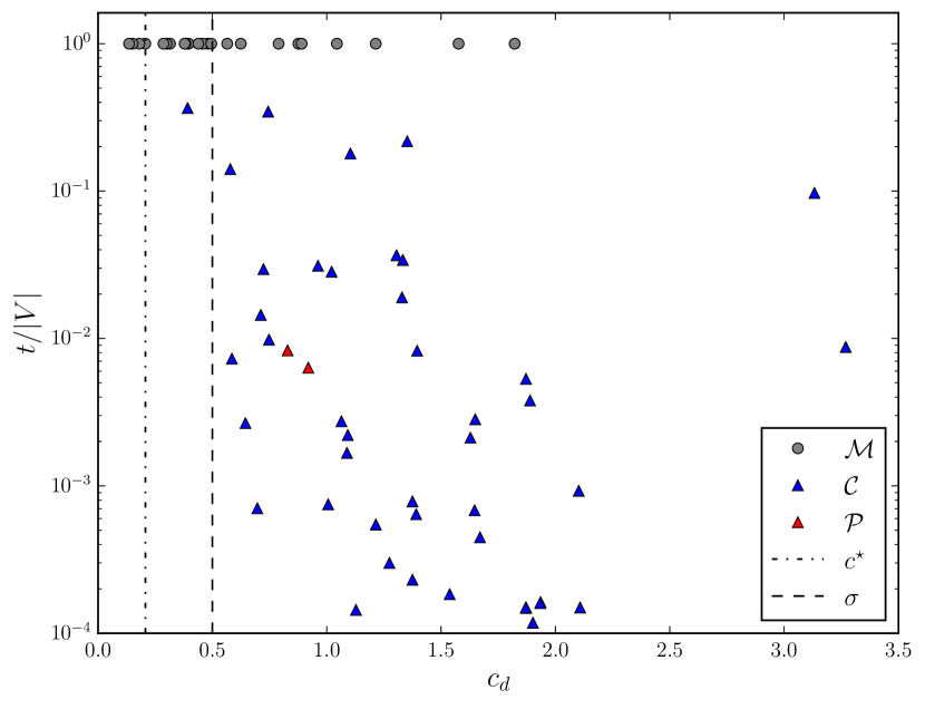
Figure 1: Almost-consensus and metastability of the experiments compared to the theoretical and empirical thresholds $c^{\star}$ and $\sigma$. In 81% of the runs there is an almost-consensus if $c_{d}>\sigma$; the 86% of them are metastable when $c_{d}<\sigma$. The value $t$ is the arithmetic mean of the number of rounds until almost-consensus/metastability was declared.

Table 1: Experimental data. Source reports the source of the dataset, i.e. SNAP (S) or KONECT (K). The values $c_{r}$ and $c_{d}$ are the robustness and dominance obtained using the densest-core method; the values $\bar{c}_{r}$ and $\bar{c}_{d}$ are the robustness and dominance obtained using the $k$-rich-club method. $\mathcal{C}$ and $\mathcal{P}$ are the fraction of experiments in which the core’s and the periphery’s color respectively spread to reach an almost-consensus, while $\mathcal{M}$ is the fraction of experiments in which there is metastability, all having the core extracted with the densest-core method. K stands for thousand, M for million.

Dataset (Source)	$|V|$	$|E|$	$c_{r}\,(\bar{c}_{r})$	$c_{d}\,(\bar{c}_{d})$	$\mathcal{C}$	$\mathcal{P}$	$\mathcal{M}$
Chicago (K)	0.8K	1.6K	6.55 (0.10)	0.15 (9.72)	0.00	0.00	1.00
email-Eu-core (S)	0.9K	32.1K	0.75 (0.53)	1.32 (1.88)	0.92	0.08	0.00
Euroroad (K)	1.0K	2.6K	5.53 (0.62)	0.18 (1.61)	0.00	0.00	1.00
Blogs (K)	1.2K	33.4K	0.62 (0.38)	1.57 (2.60)	0.00	0.00	1.00
Traffic Control (K)	1.2K	4.8K	1.25 (0.51)	0.78 (1.96)	0.00	0.00	1.00
Protein (K)	1.4K	3.8K	0.90 (0.33)	1.10 (2.95)	1.00	0.00	0.00
US Airport (K)	1.5K	34.4K	0.54 (0.48)	1.82 (2.10)	0.00	0.00	1.00
Stelzl (K)	1.6K	6.2K	1.03 (0.36)	0.96 (2.73)	1.00	0.00	0.00
Bible (K)	1.7K	18.1K	0.74 (0.54)	1.33 (1.84)	0.98	0.02	0.00
Hamster full (K)	2.0K	32.1K	0.96 (0.66)	1.02 (1.51)	1.00	0.00	0.00
Opsahl OF (K)	2.9K	31.2K	0.76 (0.55)	1.30 (1.81)	1.00	0.00	0.00
OpenFlights (K)	3.3K	38.4K	0.73 (0.50)	1.35 (1.98)	0.80	0.00	0.20
bitcoin-alpha (S)	3.7K	28.2K	0.53 (0.39)	1.87 (2.52)	1.00	0.00	0.00
ego-Facebook (S)	4.0K	176.4K	4.83 (1.53)	0.20 (0.65)	0.00	0.00	1.00
ca-GrQc (S)	4.1K	26.8K	3.33 (1.29)	0.29 (0.77)	0.00	0.00	1.00
US power grid (K)	4.9K	13.1K	3.17 (0.53)	0.31 (1.86)	0.00	0.00	1.00
bitcoin-otc (S)	5.8K	42.9K	0.52 (0.38)	1.88 (2.59)	1.00	0.00	0.00
p2p-Gnutella08 (S)	6.2K	41.5K	1.20 (0.53)	0.82 (1.86)	0.00	1.00	0.00
Route Views (K)	6.4K	25.1K	0.30 (0.16)	3.26 (6.13)	0.96	0.04	0.00
wiki-Vote (S)	7.0K	201.4K	0.60 (0.44)	1.64 (2.24)	1.00	0.00	0.00
p2p-Gnutella09 (S)	8.1K	52.0K	1.08 (0.53)	0.91 (1.86)	0.00	1.00	0.00
ca-HepPh (S)	8.6K	49.6K	1.40 (0.69)	0.71 (1.44)	1.00	0.00	0.00
p2p-Gnutella06 (S)	8.7K	63.0K	0.91 (0.53)	1.09 (1.87)	1.00	0.00	0.00
p2p-Gnutella05 (S)	8.8K	63.6K	0.93 (0.54)	1.06 (1.83)	0.86	0.14	0.00
PGP (K)	10.6K	48.6K	2.54 (1.18)	0.39 (0.84)	1.00	0.00	0.00
p2p-Gnutella04 (S)	10.8K	79.9K	0.91 (0.52)	1.08 (1.90)	1.00	0.00	0.00
ca-HepTh (S)	11.2K	235.2K	3.49 (2.39)	0.28 (0.41)	0.00	0.00	1.00
ca-AstroPh (S)	17.9K	393.9K	1.54 (0.84)	0.64 (1.18)	1.00	0.00	0.00
ca-CondMat (S)	21.3K	182.5K	1.70 (0.68)	0.58 (1.46)	1.00	0.00	0.00
p2p-Gnutella25 (S)	22.6K	109.3K	0.72 (0.41)	1.37 (2.43)	1.00	0.00	0.00
E.A.T. (K)	23.1K	594.1K	0.60 (0.48)	1.64 (2.07)	0.96	0.04	0.00
Cora citation (K)	23.1K	178.3K	1.37 (0.54)	0.72 (1.83)	1.00	0.00	0.00
CAIDA (K)	26.4K	106.7K	0.31 (0.16)	3.13 (6.03)	1.00	0.00	0.00
p2p-Gnutella24 (S)	26.4K	130.7K	0.71 (0.42)	1.39 (2.34)	1.00	0.00	0.00
cit-HepTh (S)	27.4K	704.0K	1.33 (0.74)	0.74 (1.34)	1.00	0.00	0.00
Digg (K)	29.6K	169.5K	0.59 (0.49)	1.67 (2.01)	1.00	0.00	0.00
Linux (K)	30.8K	426.4K	0.47 (0.24)	2.10 (4.14)	0.90	0.10	0.00
email-Enron (S)	33.6K	361.6K	0.71 (0.54)	1.39 (1.84)	1.00	0.00	0.00
cit-HepPh (S)	34.4K	841.5K	1.34 (0.61)	0.74 (1.61)	1.00	0.00	0.00
Internet topology (K)	34.7K	215.4K	0.61 (0.32)	1.62 (3.08)	0.88	0.00	0.12
p2p-Gnutella30 (S)	36.6K	176.6K	0.82 (0.44)	1.21 (2.23)	1.00	0.00	0.00
loc-Brightkite (S)	56.7K	425.8K	0.99 (0.71)	1.00 (1.40)	1.00	0.00	0.00
p2p-Gnutella31 (S)	62.5K	295.7K	0.78 (0.44)	1.27 (2.26)	1.00	0.00	0.00
soc-Epinions1 (S)	75.8K	811.4K	0.72 (0.60)	1.37 (1.65)	1.00	0.00	0.00
Slashdot081106 (S)	77.3K	937.1K	0.51 (0.46)	1.93 (2.13)	0.98	0.02	0.00
soc-Slashdot0811 (S)	77.3K	938.3K	0.51 (0.46)	1.93 (2.13)	1.00	0.00	0.00
ego-Twitter (S)	81.3K	2.6M	1.12 (0.57)	0.89 (1.75)	0.00	0.00	1.00
Slashdot090216 (S)	81.8K	995.3K	0.53 (0.48)	1.87 (2.08)	1.00	0.00	0.00
Slashdot090221 (S)	82.1K	1.0M	0.53 (0.48)	1.87 (2.08)	1.00	0.00	0.00
soc-Slashdot0922 (S)	82.1K	1.0M	0.53 (0.47)	1.87 (2.08)	1.00	0.00	0.00
Prosper loans (K)	89.1K	6.6M	0.82 (0.47)	1.21 (2.10)	0.00	0.00	1.00
Livemocha (K)	104.1K	4.3M	0.47 (0.38)	2.10 (2.56)	0.94	0.06	0.00
Flickr (K)	105.7K	4.6M	2.27 (1.07)	0.43 (0.92)	0.00	0.00	1.00
ego-Gplus (S)	107.6K	24.4M	0.95 (0.54)	1.04 (1.82)	0.00	0.00	1.00
epinions (S)	119.1K	1.4M	0.64 (0.52)	1.53 (1.89)	1.00	0.00	0.00
Github (K)	120.8K	879.7K	0.88 (0.70)	1.12 (1.41)	1.00	0.00	0.00
Bookcrossing (K)	185.9K	867.2K	0.52 (0.34)	1.90 (2.87)	1.00	0.00	0.00
loc-Gowalla (S)	196.5K	1.9M	1.14 (0.80)	0.87 (1.24)	0.02	0.00	0.98
email-EuAll (S)	224.8K	679.8K	0.16 (0.06)	6.19 (14.4)	0.00	0.00	1.00
web-Stanford (S)	255.2K	3.8M	2.52 (0.37)	0.39 (2.68)	0.00	0.00	1.00
amazon0302 (S)	262.1K	1.7M	2.61 (0.44)	0.38 (2.23)	1.00	0.00	0.00
com-DBLP (S)	317.0K	2.0M	1.43 (0.70)	0.69 (1.42)	1.00	0.00	0.00
web-NotreDame (S)	325.7K	2.1M	2.63 (0.60)	0.37 (1.65)	0.00	0.00	1.00
com-amazon (S)	334.8K	1.8M	1.72 (0.32)	0.57 (3.03)	0.98	0.00	0.02
amazon0312 (S)	400.7K	4.6M	2.18 (0.41)	0.45 (2.41)	0.00	0.00	1.00
amazon0601 (S)	403.3K	4.8M	2.08 (0.40)	0.47 (2.44)	0.00	0.00	1.00
amazon0505 (S)	410.2K	4.8M	2.01 (0.41)	0.49 (2.40)	0.00	0.00	1.00
web-BerkStan (S)	654.7K	13.1M	1.60 (0.43)	0.62 (2.30)	0.00	0.00	1.00
web-Google (S)	855.8K	8.5M	1.77 (0.42)	0.56 (2.33)	0.00	0.00	1.00
roadNet-PA (S)	1.0M	3.0M	7.35 (1.01)	0.13 (0.98)	0.00	0.00	1.00

As can be observed in Figure 1, there exists an empirical threshold $\sigma=\frac{1}{2}$ which is different from the theoretical one. In fact, in $81\%$ of the datasets with a dominance above the threshold the 2-Choices dynamics converges to an almost-consensus while in $86\%$ of the datasets with a dominance below the threshold, the 2-Choices dynamics ends up in a metastable phase. The empirical threshold is greater than the theoretical threshold because of several factors: (i) in the experiments the core actually changes color to a small extent (while in the theoretical part we ignored such small perturbations), and it consequently lowers the probability for an agent in the periphery to pick the core’s color; (ii) the real-world network we used in the experiments do not have the regularity assumptions of the networks that we consider in the analysis; (iii) in the experiments we declare metastability only after $|V|$ iterations and this increases the likelihood of false positive metastable runs. The gap between the theoretical and the empirical threshold should be closed in future work by providing a more fine-grained theoretical analysis which does not assume the adversary’s color to be monochromatic and considers more general networks.

We want to highlight that the protocol’s convergence to the core’s color (as shown in Table LABEL:tab:datasets) is remarkable in light of the fact that the densest-core method ensures that the sum of the agents’ degrees of the core and of the periphery are equal. More precisely, note that equal volumes of core and periphery, starting from an initial configuration where two sets support different colors, is sufficient in the Voter Model to say that the two initial colors have the same probability to be the one eventually supported by all agents [HP01], regardless of the topological structure. Previous works on the 2-Choices dynamics [CER14] provided convergence results which are parametrized only in the difference of the volumes of the two sets, suggesting a similar behavior. Our experimental results highlight the insufficiency of the initial volume distribution as an accurate predictive parameter, showing that the topological structure of the core plays a decisive role.

5 Conclusions

We analyzed the 2-Choices dynamics on a class of networks with core-periphery structure, where the core, a small group of densely interconnected agents, initially holds a different opinion from the rest of the network, the periphery. We formally proved that a phase-transition phenomenon occurs: Depending on the dominance parameter $c_{d}$ characterizing the connectivity of the network, either the core’s opinion spreads among the agents of the periphery and the network reaches an (almost-)consensus, or there is a metastability phase in which none of the opinions prevails over the other.

We validated our theoretical results on several real-world networks. Introducing an efficient and effective method to extract the core, we showed that the same parameter $c_{d}$ is sufficient to predict the convergence/metastability of the 2-Choices dynamics most of the time. Surprisingly, even if the volumes of core and periphery are equal, the core’s opinion wins in most of the cases. These behaviors suggest that in many real-world networks there actually is a core whose initial opinion has a great advantage of spreading in simple opinion dynamics such as the 2-Choices. We think that these results are a relevant step towards understanding which dynamical properties are implicitly responsible for causing social and economic agents to form networks with a core-periphery structure.

References

- [ABC+20] Aris Anagnostopoulos, Luca Becchetti, Emilio Cruciani, Francesco Pasquale, and Sara Rizzo. Biased opinion dynamics: When the devil is in the details. In Christian Bessiere, editor, Proceedings of the Twenty-Ninth International Joint Conference on Artificial Intelligence, IJCAI 2020, pages 53–59. ijcai.org, 2020.
- [ABLP17] Chen Avin, Michael Borokhovich, Zvi Lotker, and David Peleg. Distributed computing on core-periphery networks: Axiom-based design. J. Parallel Distrib. Comput., 99:51–67, 2017.
- [AF02] David Aldous and James Allen Fill. Reversible markov chains and random walks on graphs, 2002. Unfinished monograph, recompiled 2014, available at https://www.stat.berkeley.edu/users/aldous/RWG/book.html.
- [ALP+14] Chen Avin, Zvi Lotker, David Peleg, Yvonne Anne Pignolet, and Itzik Turkel. Core-Periphery in Networks: An Axiomatic Approach. arXiv:1411.2242 [physics], November 2014. arXiv: 1411.2242.
- [BCN+15] Luca Becchetti, Andrea Clementi, Emanuele Natale, Francesco Pasquale, and Riccardo Silvestri. Plurality consensus in the gossip model. In Proceedings of the 26th Annual ACM-SIAM Symposium on Discrete Algorithms (SODA’15), pages 371–390. SIAM, 2015.
- [BCN+16] Luca Becchetti, Andrea E. F. Clementi, Emanuele Natale, Francesco Pasquale, and Luca Trevisan. Stabilizing consensus with many opinions. In Proceedings of the Twenty-Seventh Annual ACM-SIAM Symposium on Discrete Algorithms, SODA 2016, Arlington, VA, USA, January 10-12, 2016, pages 620–635, 2016.
- [BCN+17] Luca Becchetti, Andrea E. F. Clementi, Emanuele Natale, Francesco Pasquale, Riccardo Silvestri, and Luca Trevisan. Simple dynamics for plurality consensus. Distributed Computing, 30(4):293–306, 2017.
- [BCN20] Luca Becchetti, Andrea Clementi, and Emanuele Natale. Consensus dynamics: An overview. SIGACT News, 51(1):58–104, March 2020.
- [BCO+16] Itai Benjamini, Siu-On Chan, Ryan O’Donnell, Omer Tamuz, and Li-Yang Tan. Convergence, unanimity and disagreement in majority dynamics on unimodular graphs and random graphs. Stochastic Processes and their Applications, 126(9):2719 – 2733, 2016.
- [BE00] Stephen P Borgatti and Martin G Everett. Models of core/periphery structures. Social Networks, 21(4):375 – 395, 2000.
- [Ber01] Eli Berger. Dynamic monopolies of constant size. Journal of Combinatorial Theory, Series B, 83(2):191 – 200, 2001.
- [BFGK16] Petra Berenbrink, Tom Friedetzky, George Giakkoupis, and Peter Kling. Efficient plurality consensus, or: The benefits of cleaning up from time to time. In 43rd International Colloquium on Automata, Languages and Programming (ICALP 2016), Rome, Italy, July 2016.
- [BGKMT16] Petra Berenbrink, George Giakkoupis, Anne-Marie Kermarrec, and Frederik Mallmann-Trenn. Bounds on the Voter Model in Dynamic Networks. In Ioannis Chatzigiannakis, Michael Mitzenmacher, Yuval Rabani, and Davide Sangiorgi, editors, 43rd International Colloquium on Automata, Languages, and Programming (ICALP 2016), volume 55 of Leibniz International Proceedings in Informatics (LIPIcs), pages 146:1–146:15, Dagstuhl, Germany, 2016. Schloss Dagstuhl–Leibniz-Zentrum fuer Informatik.
- [CDFR16] Colin Cooper, Martin E. Dyer, Alan M. Frieze, and Nicolas Rivera. Discordant voting processes on finite graphs. In 43rd International Colloquium on Automata, Languages, and Programming, ICALP 2016, July 11-15, 2016, Rome, Italy, pages 145:1–145:13, 2016.
- [CER14] Colin Cooper, Robert Elsässer, and Tomasz Radzik. The power of two choices in distributed voting. In Automata, Languages, and Programming - 41st International Colloquium, ICALP 2014, Copenhagen, Denmark, July 8-11, 2014, Proceedings, Part II, pages 435–446, 2014.
- [CER+15] Colin Cooper, Robert Elsässer, Tomasz Radzik, Nicolas Rivera, and Takeharu Shiraga. Fast consensus for voting on general expander graphs. In Distributed Computing - 29th International Symposium, DISC 2015, Tokyo, Japan, October 7-9, 2015, Proceedings, pages 248–262, 2015.
- [Cha00] Moses Charikar. Greedy Approximation Algorithms for Finding Dense Components in a Graph, pages 84–95. Springer Berlin Heidelberg, Berlin, Heidelberg, 2000.
- [CMQR21] Emilio Cruciani, Hlafo Alfie Mimun, Matteo Quattropani, and Sara Rizzo. Phase transitions of the k-majority dynamics in a biased communication model. In 22nd International Conference on Distributed Computing and Networking, ICDCN 2021, Jan 5th-8th, 2021 , Virtual Conference, page To appear, 2021.
- [CNS19] Emilio Cruciani, Emanuele Natale, and Giacomo Scornavacca. Distributed community detection via metastability of the 2-choices dynamics. In The Thirty-Third AAAI Conference on Artificial Intelligence, AAAI 2019, The Thirty-First Innovative Applications of Artificial Intelligence Conference, IAAI 2019, The Ninth AAAI Symposium on Educational Advances in Artificial Intelligence, EAAI 2019, Honolulu, Hawaii, USA, January 27 - February 1, 2019, pages 6046–6053. AAAI Press, 2019.
- [CR16] Colin Cooper and Nicolas Rivera. The linear voting model. In 43rd International Colloquium on Automata, Languages, and Programming, ICALP 2016, July 11-15, 2016, Rome, Italy, pages 144:1–144:12, 2016.
- [CRR16] Colin Cooper, Tomasz Radzik, and Nicolas Rivera. The coalescing-branching random walk on expanders and the dual epidemic process. In Proceedings of the 2016 ACM Symposium on Principles of Distributed Computing, PODC 2016, Chicago, IL, USA, July 25-28, 2016, pages 461–467, 2016.
- [CRRS17] Colin Cooper, Tomasz Radzik, Nicolas Rivera, and Takeharu Shiraga. Fast plurality consensus in regular expanders. In 31st International Symposium on Distributed Computing, DISC 2017, October 16-20, 2017, Vienna, Austria, pages 13:1–13:16, 2017.
- [Deg74] Morris H. Degroot. Reaching a consensus. Journal of the American Statistical Association, 69(345):118–121, 1974.
- [DGM+11] Benjamin Doerr, Leslie Ann Goldberg, Lorenz Minder, Thomas Sauerwald, and Christian Scheideler. Stabilizing consensus with the power of two choices. In Proceedings of the Twenty-third Annual ACM Symposium on Parallelism in Algorithms and Architectures, SPAA ’11, pages 149–158, New York, NY, USA, 2011. ACM.
- [DJ10] Easley David and Kleinberg Jon. Networks, Crowds, and Markets: Reasoning About a Highly Connected World. Cambridge University Press, New York, USA, 2010.
- [DP09] Devdatt Dubhashi and Alessandro Panconesi. Concentration of Measure for the Analysis of Randomized Algorithms. Cambridge University Press, New York, NY, USA, 1st edition, 2009.
- [EJN02] Mark E. J. Newman. Spread of epidemic disease on networks. Physical review. E, Statistical, nonlinear, and soft matter physics, 66:016128, 08 2002.
- [Fre05] John R. French. A formal theory of social power. Psychological Review, 63(3):181–194, 1956-05.
- [GJ10] Benjamin Golub and Matthew O. Jackson. Naïve learning in social networks and the wisdom of crowds. American Economic Journal: Microeconomics, 2(1):112–49, February 2010.
- [GL17] Mohsen Ghaffari and Johannes Lengler. Tight analysis for the 3-majority consensus dynamics. CoRR, abs/1705.05583, 2017.
- [GP16] Mohsen Ghaffari and Merav Parter. A polylogarithmic gossip algorithm for plurality consensus. In Proceedings of the 2016 ACM Symposium on Principles of Distributed Computing, PODC 2016, Chicago, IL, USA, July 25-28, 2016, pages 117–126, 2016.
- [Har59] Frank Harary. A criterion for unanimity in french’s theory of social power. Studies in Social Power, pages 168–182, 1959.
- [Het00] Herbert W. Hethcote. The mathematics of infectious diseases. SIAM Review, 42(4):599–653, 2000.
- [HLW06] Shlomo Hoory, Nathan Linial, and Avi Wigderson. Expander graphs and their applications. BULL. AMER. MATH. SOC., 43(4):439–561, 2006.
- [HP01] Yehuda Hassin and David Peleg. Distributed probabilistic polling and applications to proportionate agreement. Information and Computation, 171(2):248 – 268, 2001.
- [Jac21] Matthew O. Jackson. Social and Economic Networks. Princeton Univers. Press, 2010-11-21.
- [Kun13] Jérôme Kunegis. Konect: the koblenz network collection. In Proceedings of the 22nd International Conference on World Wide Web, pages 1343–1350. ACM, 2013.
- [LAH07] R. Lambiotte, M. Ausloos, and J. A. Hołyst. Majority model on a network with communities. Phys. Rev. E, 75:030101, Mar 2007.
- [Lig06] Thomas M. Liggett. Interacting Particle Systems. Springer Science & Business Media, 2012-12-06. Google-Books-ID: 7JbqBwAAQBAJ.
- [Lig09] Thomas M. Liggett. Stochastic Interacting Systems: Contact, Voter and Exclusion Processes. Springer Science & Business Media, 2013-03-09. Google-Books-ID: wRv2CAAAQBAJ.
- [LK14] Jure Leskovec and Andrej Krevl. SNAP Datasets: Stanford large network dataset collection. http://snap.stanford.edu/data, June 2014.
- [LP17] David A Levin and Yuval Peres. Markov chains and mixing times, volume 107. American Mathematical Society, 2017.
- [MNT14] Elchanan Mossel, Joe Neeman, and Omer Tamuz. Majority dynamics and aggregation of information in social networks. Autonomous Agents and Multi-Agent Systems, 28(3):408–429, May 2014.
- [MT17] Elchanan Mossel and Omer Tamuz. Opinion exchange dynamics. Probab. Surveys, 14:155–204, 2017.
- [Pel98] David Peleg. Size bounds for dynamic monopolies. Discrete Applied Mathematics, 86(2-3):263–273, 1998.
- [Pel02] David Peleg. Local majorities, coalitions and monopolies in graphs: a review. Theor. Comput. Sci., 282(2):231–257, 2002.
- [RPFM14] M. Puck Rombach, Mason A. Porter, James H. Fowler, and Peter J. Mucha. Core-periphery structure in networks. SIAM Journal on Applied Mathematics, 74(1):167–190, 2014.
- [SK79] David Snyder and Edward L. Kick. Structural position in the world system and economic growth, 1955-1970: A multiple-network analysis of transnational interactions. American Journal of Sociology, 84(5):1096–1126, 1979.
- [SS19] Nobutaka Shimizu and Takeharu Shiraga. Phase transitions of best-of-two and best-of-three on stochastic block models. In Jukka Suomela, editor, 33rd International Symposium on Distributed Computing, DISC 2019, October 14-18, 2019, Budapest, Hungary, volume 146 of LIPIcs, pages 32:1–32:17. Schloss Dagstuhl - Leibniz-Zentrum für Informatik, 2019.
- [ZM04] Shi Zhou and Raúl J Mondragón. The rich-club phenomenon in the internet topology. IEEE Communications Letters, 8(3):180–182, 2004.
- [ZMN15] Xiao Zhang, Travis Martin, and M. E. J. Newman. Identification of core-periphery structure in networks. Phys. Rev. E, 91:032803, Mar 2015.