Topology-induced Enhancement of Mappings

Abstract.

In this paper we propose a new method to enhance a mapping $\mu(\cdot)$ of a parallel application’s computational tasks to the processing elements (PEs) of a parallel computer. The idea behind our method TiMEr is to enhance such a mapping by drawing on the observation that many topologies take the form of a partial cube. This class of graphs includes all rectangular and cubic meshes, any such torus with even extensions in each dimension, all hypercubes, and all trees.

Following previous work, we represent the parallel application and the parallel computer by graphs $G_{a}=(V_{a},E_{a})$ and $G_{p}=(V_{p},E_{p})$. $G_{p}$ being a partial cube allows us to label its vertices, the PEs, by bitvectors such that the cost of exchanging one unit of information between two vertices $u_{p}$ and $v_{p}$ of $G_{p}$ amounts to the Hamming distance between the labels of $u_{p}$ and $v_{p}$.

By transferring these bitvectors from $V_{p}$ to $V_{a}$ via $\mu^{-1}(\cdot)$ and extending them to be unique on $V_{a}$, we can enhance $\mu(\cdot)$ by swapping labels of $V_{a}$ in a new way. Pairs of swapped labels are local w. r. t. the PEs, but not w. r. t. $G_{a}$. Moreover, permutations of the bitvectors’ entries give rise to a plethora of hierarchies on the PEs. Through these hierarchies we turn TiMEr into a hierarchical method for improving $\mu(\cdot)$ that is complementary to state-of-the-art methods for computing $\mu(\cdot)$ in the first place.

In our experiments we use TiMEr to enhance mappings of complex networks onto rectangular meshes and tori with 256 and 512 nodes, as well as hypercubes with 256 nodes. It turns out that common quality measures of mappings derived from state-of-the-art algorithms can be improved considerably.

1. Introduction

Large-scale matrix- or graph-based applications such as numerical simulations (Trobec and Kosec, 2015) or massive network analytics (Que et al., 2015) often run on parallel systems with distributed memory. The iterative nature of the underlying algorithms typically requires recurring communication between the processing elements (PEs). To optimize the running time of such an application, the computational load should be evenly distributed onto the PEs, while at the same time, the communication volume between them should be low. When mapping processes to PEs on non-uniform memory access (NUMA) systems, it should also be taken into account that the cost for communication operations depends on the locations of the PEs involved. In particular, one wants to map heavily communicating processes “close to each other”.

More formally, let the application be modeled by an application graph $G_{a}=(V_{a},E_{a},\omega_{a})$ that needs to be distributed over the PEs. A vertex in $V_{a}$ represents a computational task of the application, while an edge $e_{a}=\{u_{a},v_{a}\}$ indicates data exchanges between tasks $u_{a}$ and $v_{a}$, with $\omega_{a}(e_{a})$ specifying the amount of data to be exchanged. The topology of the parallel system is modeled by a processor graph $G_{p}=(V_{p},E_{p},\omega_{p})$, where the edge weight $\omega_{p}(\{u_{p},v_{p}\})$ indicates the cost of exchanging one data unit between the PEs $u_{p}$ and $v_{p}$ (Deveci et al., 2015; Glantz et al., 2015). A balanced distribution of processes onto PEs thus corresponds to a mapping $\mu:V_{a}\mapsto V_{p}$ such that, for some small $\varepsilon\geq 0$,

(1) $$|\mu^{-1}(v_{p})|\leq(1+\varepsilon)\cdot\lceil|V_{a}|/|\mu(V_{a})|\rceil$$

for all $v_{p}\in\mu(V_{a})$. Therefore, $\mu(\cdot)$ induces a balanced partition of $G_{a}$ with blocks $\mu^{-1}(v_{p})$, $v_{p}\in V_{p}$. Conversely, one can find a mapping $\mu:V_{a}\mapsto V_{p}$ that fulfills Eq. (1) by first partitioning $V_{a}$ into $|V_{p}|$ balanced parts (Bichot and Siarry, 2011) and then specifying a one-to-one mapping from the blocks of the partition onto the vertices of $G_{p}$. For an accurate modeling of communication costs, one would also have to specify the path(s) over which two vertices communicate in $G_{p}$. This is, however, system-specific. For the purpose of generic algorithms, it is thus often abstracted away by assuming routing on shortest paths in $G_{p}$  (Hoefler and Snir, 2011). In this work, we make the same assumption.

In order to steer an optimization process for obtaining good mappings, different objective functions have been proposed (Hoefler and Snir, 2011; Kim and Lai, 1991; Deveci et al., 2015). One of the most commonly used (Pellegrini, 2011) objective functions is $\operatorname{Coco}(\cdot)$ (also referred to as hop-byte in (Yu et al., 2006)), cf. Eq. (3):

(2) $$\mu^{*} :=\operatorname{argmin}\limits_{\begin{subarray}{c}\mu:V_{a}\mapsto V_{p}\\ \mu\mbox{\tiny~{}balanced}\end{subarray}}\operatorname{Coco}(\mu)\mbox{, with}$$

(3) $$\operatorname{Coco}(\mu) :=\sum_{\begin{subarray}{c}\mathbf{e}_{a}\in E_{a}\\ {\mbox{\tiny$e_{a}=\{u_{a},v_{a}\}$}}\end{subarray}}\omega_{a}(e_{a})~{}d_{G_{p}}(\mu(u_{a}),\mu(v_{a})),$$

where $d_{G_{p}}(\mu(u_{a}),\mu(v_{a}))$ denotes the distance between $\mu(u_{a})$ and $\mu(v_{a})$ in $G_{p}$, i. e. the number of edges on shortest paths. Broadly speaking, $\operatorname{Coco}(\cdot)$ is minimised when pairs of highly communicating processes are placed in nearby processors. Finding $\mu^{*}(\cdot)$ is $\mathcal{NP}$-hard. Indeed, finding $\mu^{*}(\cdot)$ for a complete graph $G_{p}$ amounts to graph partitioning, which is an $\mathcal{NP}$-hard problem (Garey and Johnson, 1979).

Related work and motivation

One way of looking at previous algorithmic work from a high-level perspective (more details can be found in the overview articles by Pellegrini (Pellegrini, 2011), Buluç et al. (Buluç et al., 2016), and Aubanel (Aubanel, 2009)) is to group it into two categories. One line has tried to couple mapping with graph partitioning. To this end, the objective function for partitioning, usually the edge cut, is replaced by an objective function like $\operatorname{Coco}(\cdot)$ that considers distances $d_{G_{p}}(\cdot)$ (Walshaw and Cross, 2001). To avoid recomputing these values, Walshaw and Cross (Walshaw and Cross, 2001) store them in a network cost matrix (NCM). When our proposed method TiMEr (Topology-induced Mapping Enhancer) is used to enhance a mapping, it does so without an NCM, thus avoiding its quadratic space complexity.

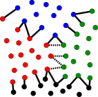
The second line of research decouples partitioning and mapping. First, $G_{a}$ is partitioned into $|G_{p}|$ blocks without taking $G_{p}$ into account. Typically, this step involves multilevel approaches whose hierarchies on $G_{a}$ are built with edge contraction (Karypis and Kumar, 1998; Osipov and Sanders, 2010; Sanders and Schulz, 2013a) or weighted aggregation (Chevalier and Safro, 2009; Meyerhenke et al., 2009). Contraction of the blocks of $G_{a}$ into single vertices yields the communication graph $G_{c}=(V_{c},E_{c},\omega_{c})$, where $\omega_{c}(e_{c})$, $e_{c}\in E_{c}$, aggregates the weight of edges in $G_{a}$ with end vertices in different blocks. For an example see Figures 1a,1b. Finally, one computes a bijection $\nu:V_{c}\mapsto V_{p}$ that minimizes $\operatorname{Coco}(\cdot)$ or a related function, using (for example) greedy methods (Hoefler and Snir, 2011; Brandfass et al., 2013; Glantz et al., 2015; Deveci et al., 2015) or metaheuristics (Brandfass et al., 2013; Ucar et al., 2006), see Figure 1c. When TiMEr is used to enhance such a mapping, it modifies not only $\nu(\cdot)$, but also affects the partition of $V_{a}$ (and thus possibly $G_{c}$). Hence, deficiencies due to the decoupling of partitioning and mapping can be compensated. Note that, since TiMEr is proposed as an improvement on mappings derived from state-of-the-art methods, we assume that an initial mapping is provided. This is no limitation: a mapping can be easily computed from the solution of a graph partitioner using the identity mapping from $G_{c}$ to $G_{p}$.

(a) $G_{a}$

(b) $G_{c}$

(c) $G_{p}$

Figure 1. (a) Application graph partitioned into four blocks with unitary edge weights. (b) Resulting communication graph, numbers indicate edge weights. (c) The processor graph is a partial cube and the bijection $\nu(\cdot)$ between the vertices of $G_{c}$ and those of $G_{p}$ is indicated by the colors. Communication between the red and the green vertex has to be routed via an intermediary node (the blue one or the black one).

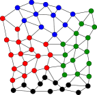
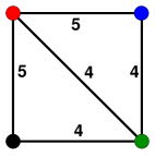
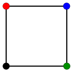
Being man-made and cost-effective, the topologies of parallel computers exhibit special properties that can be used to find good mappings. A widely used property is that PEs are often “hierarchically organized into, e. g., islands, racks, nodes, processors, cores with corresponding communication links of similar quality” (Schulz and Träff, 2017). Thus, dual recursive bisection (DRB) (Pellegrini, 1994), the recent embedded sectioning (Kirmani et al., 2017), and what can be called recursive multisection (Chan et al., 2012; Jeannot et al., 2013; Schulz and Träff, 2017) suggest themselves for mapping: DRB and embedded sectioning cut both $G_{a}$ (or $G_{c}$) and $G_{p}$ into two blocks recursively and assign the respective blocks to each other in a top-down manner. Recursive multisection as performed by (Schulz and Träff, 2017) models the hierarchy inherent in $G_{p}$ as a tree. The tree’s fan-out then determines into how many blocks $G_{c}$ needs to be partitioned. Again, TiMEr is complementary in that we do not need an actual hierarchy of the topology.

Overview of our method.

To the best of our knowledge, TiMEr is the first method to exploit the fact that many parallel topologies are partial cubes. A partial cube is an isometric subgraph of a hypercube, see Section 2 for a formal definition. This graph class includes all rectangular and cubic meshes, any such torus with even extensions in each dimension, all hypercubes, and all trees.

$G_{p}$ being a partial cube allows us to label its vertices with bitvectors such that the distance between two vertices in $G_{p}$ amounts to the Hamming distance (number of different bits) between the vertices’ labels (see Sections 2 and 3). This will allow us to compute the contribution of an edge $e_{a}\in E_{a}$ to $\operatorname{Coco}(\cdot)$ quickly. The labels are then extended to labels for vertices in $G_{a}$ (Section 4). More specifically, a label of a vertex $v_{a}\in V_{a}$ consists of a left and a right part, where the left part encodes the mapping $\mu(\cdot):V_{a}\mapsto V_{p}$ and the right part makes the labels unique. Note that it can be instructive to view the vertex labels of $V_{a}$, $l_{a}(\cdot)$, as a recursive bipartitioning of $V_{a}$: the $i$-th leftmost bit of $l_{a}(v_{a})$ defines whether $v_{a}$ belongs to one or the other side of the corresponding cut in the $i$-th recursion level. Vertices $u_{a},v_{a}\in V_{a}$ connected by an edge with high weight should then be assigned labels that share many of the bits in the left part.

We extend the objective function $\operatorname{Coco}(\cdot)$ by a factor that accounts for the labels’ right part and thus for the uniqueness of the label, We do so without limiting the original objective that improves the labels’ left part (and thus $\mu(\cdot)$) (Section 5). Finally, we use the labeling of $V_{a}$ to devise a multi-hierarchical search method in which label swaps improve $\mu(\cdot)$. One can view this as a solution method for finding a $\operatorname{Coco}(\cdot)$-optimal numbering of the vertices in $V_{a}$, where the numbering is determined by the labels.

Compared to simple hill-climbing methods, we increase the local search space by employing very diverse hierarchies. These hierarchies result from random permutations of the label entries; they are imposed on the vertices of $G_{p}$ and built by label contractions performed digit by digit. This approach provides a fine-to-coarse view during the optimization process (Section 6) that is orthogonal to typical multilevel graph partitioning methods.

Experimental results.

As the underlying application for our experiments, we assume parallel complex network analysis on systems with distributed memory. Thus, in Section 7, we apply TiMEr to further improve mappings of complex networks onto partial cubes with 256 and 512 nodes. The initial mappings are computed using KaHIP (Sanders and Schulz, 2013b), Scotch (Pellegrini, 2007) and LibTopoMap (Hoefler and Snir, 2011). To evaluate the quality results of TiMEr, we use $\operatorname{Coco}(\cdot)$, for which we observe a relative improvement from 6% up to 34%, depending on the choice of the initial mapping. Running times for TiMEr are on average 42% faster than the running times for partitioning the graphs with KaHIP.

2. Partial cubes and their hierarchies

The graph-theoretical concept of a partial cube is central for this paper. Its definition is based on the hypercube.

Definition 2.1 (Hypercube).

A $dim_{H}$-dimensional hypercube $H$ is the graph $H(V_{H},E_{H})$ with $V_{H}:=\{0,1\}^{dim_{H}}$ and $E_{H}:=\{\{u_{H},w_{H}\}\mid u_{H},v_{H}\in V_{H}\mbox{~{}and~{}}d_{h}(u_{H},v_{H})=1\}$, where $d_{h}(u_{H},v_{H})$ denotes the Hamming distance (number of different bits) between $u_{H}$ and $v_{H}$.

More generally, $d_{H}(u_{H},v_{H})=d_{h}(u_{H},v_{H})$, i. e., the (unweighted) shortest path length equals the Hamming distance in a hypercube.

Partial cubes are isometric subgraphs of hypercubes, i. e., the distance between any two nodes in a partial cube is the same as their distance in the hypercube. Put differently:

Definition 2.2 (Partial cube).

A graph $G_{p}$ with vertex set $V_{p}$ is a partial cube of dimension $dim_{G_{p}}$ if (i) there exists a labeling $l_{p}:V_{p}\mapsto\{0,1\}^{dim_{G_{p}}}$ such that $d_{G_{p}}(u_{p},v_{p})=d_{h}(l_{p}(u_{p}),l_{p}(v_{p}))$ for all $u_{p},v_{p}\in V_{p}$ and (ii) $dim_{G_{p}}$ is as small as possible.

The labeling $l_{p}~{}:~{}V_{p}\mapsto\{0,1\}^{dim_{G_{p}}}$ gives rise to hierarchies on $V_{p}$ as follows. For any permutation $\pi$ of $\{1,\dots,dim_{G_{p}}\}$, one can group the vertices in $V_{p}$ by means of the equivalence relations $\sim_{\pi,i}$, where $dim_{G_{p}}\geq i\geq 1$:

(4) $$u_{p}\sim_{\pi,i}v_{p}:\Leftrightarrow\pi(l_{p}(u_{p}))[j]=\pi(l_{p}(v_{p}))[j]$$

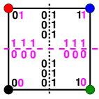
for all $1\leq j\leq i$ (where $l[i]$ refers to the $i$-th character in string $l$). As an example, $\sim_{id,i}$, where $id$ is the identity on $\{0,1\}^{dim_{G_{p}}}$, gives rise to the partition in which $u_{p}$ and $v_{p}$ belong to the same part if and only if their labels agree at the first $i$ positions. More generally, for each permutation $\pi(\cdot)$ from the set $\Pi_{dim_{G_{p}}}$ of all permutations on $\{1,\dots,dim_{G_{p}}\}$, the equivalence relations $\sim_{\pi,i}$, $dim_{G_{p}}\geq i\geq 1$, give rise to a hierarchy of increasingly coarse partitions $(\mathcal{P}_{dim_{G_{p}}},\dots,\mathcal{P}_{1})$. As an example, the hierarchies defined by the permutations $id$ and $\pi(j):=dim_{G_{p}}+1-j$, $1\leq j\leq dim_{G_{p}}$, respectively, are opposite hierarchies, see Figure 2.

Figure 2. Two opposite hierarchies of the 4D hypercube. “x” means “$0$” or “$1$”. Top: hierarchy $H_{\pi}$ with $\pi=(1,2,3,4)$. Bottom: hierarchy $H_{\pi}$ with $\pi=(4,3,2,1)$.

3. Vertex labels of processor graph

In this section we provide a way to recognize if a graph $G_{p}$ is a partial cube, and if so, we describe how a labeling on $V_{p}$ can be obtained in $\mathcal{O}(|E_{p}|^{2})$ time. To this end, we characterize partial cubes in terms of (cut-sets of) convex cuts.

Definition 3.1 (Convex cut).

Let $G_{p}=(V_{p},E_{p})$ be a graph, and let $(V_{p}^{0},V_{p}^{1})$ be a cut of $G_{p}$. The cut is called convex if no shortest path from a vertex in $V_{p}^{0}$ [$V_{p}^{1}$] to another vertex in $V_{p}^{0}$ [$V_{p}^{1}$] contains a vertex of $V_{p}^{1}$ [$V_{p}^{0}$].

The cut-set of a cut $(V_{p}^{0},V_{p}^{1})$ of $G_{p}$ consists of all edges in $G_{p}$ with one end vertex in $V_{p}^{0}$ and the other one in $V_{p}^{1}$. Given the above definitions, $G_{p}$ is a partial cube if and only if (i) $G_{p}$ is bipartite and (ii) the cut-sets of $G_{p}$’s convex cuts partition $E_{p}$ (Ovchinnikov, 2008). In this case, the equivalence relation behind the partition is the Djoković relation $\theta$ (Ovchinnikov, 2008). Let $e_{p}=\{x_{p},y_{p}\}\in E_{p}$. An edge $f_{p}$ is Djoković related to $e_{p}$ if one of $f_{p}$’s end vertices is closer to $x_{p}$ than to $y_{p}$, while the other end vertex of $f_{p}$ is closer to $y_{p}$ than to $x_{p}$. Formally,

$$e_{p}~{}\theta~{}f_{p} :\Leftrightarrow|f_{p}\cap W_{x_{p},y_{p}}|=|f_{p}\cap W_{y_{p},x_{p}}|=1\mbox{~{}, where}$$

$$W_{x_{p},y_{p}} =\{w_{p}\in V_{p}\mid d_{G_{p}}(w_{p},x_{p})<d_{G_{p}}(w_{p},y_{p})\}.$$

Consequently, no pair of edges on any shortest path of $G_{p}$ is Djoković related. In the following, we use the above definitions to find out whether $G_{p}$ is a partial cube and, if so, to compute a labeling $l_{p}~{}:~{}V_{p}\mapsto\{0,1\}^{dim_{G_{p}}}$ for $V_{p}$ according to Definition 2.2:

1. Test whether $G_{p}$ is bipartite (in asymptotic time $\mathcal{O}(|E_{p}|)$). If $G_{p}$ is not bipartite, it is not a partial cube.

2. Pick an arbitrary edge $e_{p}^{1}$ and compute the edge set $E_{p}(e_{p}^{1},\theta):=\{f_{p}\in E_{p}~{}\mid~{}f_{p}~{}\theta~{}e_{p}^{1}\}$.

3. Keep picking edges $e_{p}^{2},e_{p}^{3},\dots$ that are not contained in an edge set computed so far and compute the edge sets $E_{p}(e_{p}^{2},\theta),$ $E_{p}(e_{p}^{3},\theta)$, $\dots$. If there is an overlap with a previous edge set, $G_{p}$ is not a partial cube.

4. While calculating $E_{p}(e_{p}^{j},\theta)$ where $1\leq j\leq dim_{G_{p}}$, set

   (5) $$l_{p}[j](u_{p}):=\begin{cases}0,&\text{if $u_{p}\in W_{x_{p}^{j},y_{p}^{j}}$}.\\ 1,&\text{otherwise}.\end{cases}$$

   For an example of such vertex labels see Figure 3a.

(a) Processor graph $G_{p}$

(b) Distances in $G_{p}$

(c) Application graph $G_{a}$

Figure 3. $G_{p}$ is a partial cube with two convex cuts: the dotted vertical cut and the dashed horizontal cut (3a). First [second] digit of vertex labels $l_{p}(\cdot)$ indicates position w. r. t. vertical [horizontal] cut. Distance between $u_{p}$ and $v_{p}$ in $G_{p}$ equals Hamming distance between $l_{p}(u_{p})$ and $l_{p}(v_{p})$ (3b). In 3c, a mapping $\mu(\cdot)$ from $V_{a}$ to $V_{p}$’ is indicated by the colors. Communication across solid [dashed] edges requires 1 hop [2 hops] in $G_{p}$.

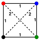
Assuming that all distances between node pairs are computed beforehand, calculating $E_{p}(e_{p}^{j},\theta)$ for $1\leq j\leq dim_{G_{p}}$ and setting the labeling $l_{p}(\cdot)$ (in steps $2$,$3$ and $4$) take $\mathcal{O}(|E_{p}|)$ time. Detecting overlaps with already calculated edge sets takes $\mathcal{O}(|E_{p}|^{2})$ time (in step $3$), which summarizes the time complexity of the proposed method.

Note that the problem has to be solved only once for a parallel computer. Since $|E_{p}|=\mathcal{O}(|V_{p}|)$ for 2D/3D grids and tori – the processor graphs of highest interest in this paper – and $|E_{p}|=\mathcal{O}(|V_{p}|\log{|V_{p}|})$ for all partial cubes, our simple method is (almost) as fast, asymptotically, as the fastest and rather involved methods that solve the problem. Indeed, the fastest method to solve the problem takes time $\mathcal{O}(|V_{p}||E_{p}|)$ (Imrich, 1993). Assuming that integers of at least $\log_{2}(|V_{p}|)$ bits can be stored in a single machine word and that addition, bitwise Boolean operations, comparisons and table look-ups can be performed on these words in constant time, the asymptotic time is reduced to $\mathcal{O}(|V_{p}|^{2})$ (Eppstein, 2011).

4. Vertex labels of application graph

Given an application graph $G_{a}=(V_{a},E_{a},\omega_{a}(\cdot))$, a processor graph $G_{p}=(V_{p},E_{p})$ that is a partial cube and a mapping $\mu:V_{a}\mapsto V_{p}$, the aim of this section is to define a labeling $l_{a}(\cdot)$ of $V_{a}$. This labeling is then used later to improve $\mu(\cdot)$ w. r. t. Eq. (3) by swapping labels between vertices of $G_{a}$. In particular, for any $u_{a},v_{a}\in V_{a}$, the effect of their label swap on $\mu(\cdot)$ should be a function of their labels and those of their neighbors in $G_{a}$. It turns out that being able to access the vertices of $G_{a}$ by their (unique) labels is crucial for the efficiency of our method. The following requirements on $l_{a}(\cdot)$ meet our needs.

1. $l_{a}(\cdot)$ encodes $\mu(\cdot)$.

2. For any two vertices $u_{a},v_{a}\in G_{a}$, we can derive the distance between $\mu(u_{a})$ and $\mu(v_{a})$ from $l_{a}(u_{a})$ and $l_{a}(v_{a})$. Thus, for any edge $e_{a}$ of $G_{a}$, we can find out how many hops it takes in $G_{p}$ for its end vertices to exchange information, see Figure 3c.

3. The labels are unique on $V_{a}$.

To compute such $l_{a}(\cdot)$, we first transport labeling $l_{p}(\cdot)$ from $V_{p}$ to $V_{a}$ through $l_{p}(v_{a}):=l_{p}(\mu(v_{a}))$ for all $v_{a}\in V_{a}$. This new labeling $l_{p}:~{}V_{a}\mapsto\{0,1\}^{dim_{G_{p}}}$ already fulfills items 1) and 2). Indeed, item 1) holds, since labels are unique on $V_{p}$; item 2) holds, because $G_{p}$ is a partial cube. To fulfill item 3), we extend the labeling $l_{p}:V_{a}\mapsto\{0,1\}^{dim_{G_{p}}}$ to a labeling $l_{a}:V_{a}\mapsto\{0,1\}^{dim_{G_{a}}}$, where yet undefined $dim_{G_{a}}$ should exceed $dim_{G_{p}}$ only by the smallest amount necessary to ensure that $l_{a}(u_{a})\neq l_{a}(v_{a})$ whenever $u_{a}\neq v_{a}$. The gap $dim_{G_{a}}-dim_{G_{p}}$ depends on the size of the largest part in the partition induced by $\mu(\cdot)$.

Definition 4.1 ($dim_{G_{a}}$).

Let $\mu:V_{a}\mapsto V_{p}$ be a mapping. We set:

(6) $$dim_{G_{a}}=dim_{G_{a}}(\mu)=dim_{G_{p}}+\max_{v_{p}\in V_{p}}\lceil\log_{2}|\mu^{-1}(v_{p})|\rceil.$$

For any $v_{a}\in V_{a}$, $l_{a}(v_{a})$ is a bitvector of length $dim_{G_{a}}$; its first $dim_{G_{p}}$ entries coincide with $l_{p}(v_{a})$, see above, and its last $dim_{G_{a}}-dim_{G_{p}}$ entries serve to make the labeling unique. We denote the bitvector formed by the last $dim_{G_{a}}-dim_{G_{p}}$ entries by $l_{e}(v_{a})$. Here, the subscript $e$ in $l_{e}(\cdot)$ stands for “extension”. To summarize,

(7) $$l_{a}(v_{a})=l_{p}(v_{a})\circ l_{e}(v_{a})\mbox{~{}~{}for all $v_{a}\in V_{a}$},\text{where}$$

$\circ$ stands for concatenation. Except for temporary permutations of the labels’ entries, the set $\mathcal{L}:=l(V_{a})$ of labels will remain the same. A label swap between $u_{a}$ and $v_{a}$ alters $\mu(\cdot)$ if and only if $l_{p}(u_{a})\neq l_{p}(v_{a})$. The balance of the partition of $V_{a}$, as induced by $\mu(\cdot)$, is preserved by swapping the labels of $V_{a}$.

Computing $l_{e}(\cdot)$ is straightforward. First, the vertices in each $\mu^{-1}(v_{p})$, $v_{p}\in V_{p}$, are numbered from $0$ to $|\mu^{-1}(v_{p})|-1$. Second, these decimal numbers are then interpreted as bitvectors/binary numbers. Finally, the entries of the corresponding bitvectors are shuffled, so as to provide a good random starting point for the improvement of $\mu$, see Lemma 5.1 in Section 5.

5. Extension of the objective function

Given the labeling of vertices in $V_{a}$, i. e., $l_{a}(\cdot)=l_{p}(\cdot)\circ l_{e}(\cdot)$, it is easy to see that solely $l_{p}(\cdot)$ determines the value of $\operatorname{Coco}(\cdot)$. (This fact results from $l_{p}(\cdot)$ encoding the distances between vertices in $G_{p}$.) On the other hand, due to the uniqueness of the labels $l_{a}(\cdot)$, $l_{e}(\cdot)$ restricts $l_{p}(\cdot)$: $l_{e}(u_{a})=l_{e}(v_{a})$ implies $l_{p}(u_{a})\neq l_{p}(v_{a})$, i. e., that $u_{a}$ and $v_{a}$ are mapped to different PEs.

The plan of the following is to ease this restriction by avoiding as many cases of $l_{e}(u_{a})=l_{e}(v_{a})$ as possible. To this end, we incorporate $l_{e}(\cdot)$ into the objective function, thus replacing $\operatorname{Coco}(\cdot)$ by a modified one. Observe that $l_{p}(\cdot)$ and $l_{e}(\cdot)$ give rise to two disjoint subsets of $E_{a}$, i. e. subsets of edges, the two end vertices of which agree on $l_{p}(\cdot)$ and $l_{e}(\cdot)$, respectively:

$$E_{a}^{p}=E_{a}^{p}(l_{a}) :=\{e_{a}=\{u_{a},v_{a}\}\in E_{a}\mid l_{p}(u_{a})=l_{p}(v_{a})\},$$

$$E_{a}^{e}=E_{a}^{e}(l_{a}) :=\{e_{a}=\{u_{a},v_{a}\}\in E_{a}\mid l_{e}(u_{a})=l_{e}(v_{a})\}.$$

In general these two sets do not form a partition of $E_{a}$, since there can be edges whose end vertices disagree both on $l_{p}(\cdot)$ and on $l_{e}(\cdot)$. With $h(\cdot,\cdot)$ denoting the Hamming distance, optimizing $\operatorname{Coco}(\cdot)$ in Eq. (3) can be rewritten as follows. Find

(8) $$l_{a}^{*} :=\operatorname{argmin}\limits_{\begin{subarray}{c}l_{a}:V_{a}\mapsto\mathcal{L}\\ \mbox{\tiny$l_{a}$~{}bijective}\end{subarray}}\operatorname{Coco}(l_{a})\mbox{, where}$$

(9) $$\operatorname{Coco}(l_{a}) :=\sum_{\begin{subarray}{c}e_{a}\in E_{a}\setminus E_{a}^{p}(l_{a})\\ {\mbox{\tiny$e_{a}=\{u_{a},v_{a}\}$}}\end{subarray}}\omega_{a}(e_{a})~{}h(l_{p}(u_{a}),l_{p}(v_{a})).$$

For all $e_{a}=\{u_{a},v_{a}\}\in E_{a}^{e}$ it follows that $l_{p}(u_{a})\neq l_{p}(v_{a})$, implying that $u_{a}$ and $v_{a}$ are mapped to different PEs. Thus, any edge $e_{a}\in E_{a}^{e}(l_{a})$ increases the value of $\operatorname{Coco}(\cdot)$ with a damage of

(10) $$\omega_{a}(u_{a},v_{a})~{}h(l_{p}(u_{a}),l_{p}(v_{a}))>0.$$

This suggests that reducing $E_{a}^{e}$ may be good for minimizing $\operatorname{Coco}(\cdot)$. The crucial question here is whether reducing $E_{a}^{e}$ can obstruct our primary goal, i. e., growing $E_{a}^{p}$ (see Eq. (9)). Lemma 5.1 below shows that this is not the case, at least for perfectly balanced $\mu(\cdot)$. A less technical version of Lemma 5.1 is the following: If $\mu(\cdot)$ is perfectly balanced, then two mappings, where one has bigger $E_{a}^{p}$ and one has smaller $E_{a}^{e}$ (both w. r. t. set inclusion), can be combined to a third mapping that has the bigger $E_{a}^{p}$ and the smaller $E_{a}^{e}$. The third mapping provides better prospects for minimizing $\operatorname{Coco}(\cdot)$ than the mapping from which it inherited big $E_{a}^{p}$, as, due to smaller $E_{a}^{e}$, the third mapping is less constrained by the uniqueness requirement:

Lemma 5.1 (Reducing $E_{a}^{e}$ compatible with growing $E_{p}^{e}$).

Let $\mu:V_{a}\mapsto V_{p}$ be such that $|\mu^{-1}(u_{p})|=|\mu^{-1}(v_{p})|$ for all $u_{p},v_{p}\in V_{p}$ (perfect balance). Furthermore, let $l_{a}(\cdot)$ and $l_{a}^{\prime}(\cdot)$ be bijective labelings $V_{a}\mapsto\mathcal{L}$ that correspond to $\mu(\cdot)$ as specified in Section 4. Then, $E_{a}^{p}(l_{a})\supseteq E_{a}^{p}(l_{a}^{\prime})$ and $E_{a}^{e}(l_{a}^{\prime})\subseteq E_{a}^{e}(l_{a})$ implies that there exists $l_{a}^{*}$ that also corresponds to $\mu(\cdot)$ with (i) $E_{a}^{p}(l_{a}^{*})=E_{a}^{p}(l_{a})$ and (ii) $E_{a}^{e}(l_{a}^{*})=E_{a}^{e}(l_{a}^{\prime})$.

Proof.

Set $l_{a}^{*}(\cdot):=l_{a}^{p}(\cdot)\circ l_{a}^{e}(\cdot)$. Then, $l_{a}^{*}(\cdot)$ fulfills (i) and (ii) in the claim, and the first $dim_{G_{p}}$ entries of $\mu(\cdot)$ specify $\mu(\cdot)$. If remains to show that the labeling $l_{a}^{*}(\cdot)$ is unique on $V_{a}$. This is a consequence of (a) $l_{a}(\cdot)$ being unique and (b) $E_{a}^{e}(l_{a}^{*})=E_{a}^{e}(l_{a}^{\prime})\subseteq E_{a}^{e}(l_{a})$. ∎

In practice we usually do not have perfect balance. Yet, the balance is typically low, e. g. $\epsilon=0.03$. Thus, we still expect that having small $E_{a}^{e}(l_{a})$ is beneficial for minimizing $\operatorname{Coco}(\cdot)$.

Minimization of the damage to $\operatorname{Coco}(\cdot)$ from edges in $E_{a}^{e}(l_{a})$, see Eq. (10), amounts to maximizing the diversity of the label extensions in $G_{a}$. Formally, in order to diversify, we want to find

(11) $$l_{a}^{*} :=\operatorname{argmax}\limits_{\begin{subarray}{c}l_{a}:V_{a}\mapsto\mathcal{L}\\ \mbox{\tiny$l_{a}$~{}bijective}\end{subarray}}\operatorname{Div}(l_{a})\mbox{, where}$$

(12) $$\operatorname{Div}(l_{a}) :=\sum_{\begin{subarray}{c}e_{a}\in E_{a}\setminus E_{a}^{e}(l_{a})\\ {\mbox{\tiny$e_{a}=\{u_{a},v_{a}\}$}}\end{subarray}}\omega_{a}(e_{a})~{}h(l_{e}(u_{a}),l_{e}(v_{a})).$$

We combine our two objectives, i. e., minimization of $\operatorname{Coco}(\cdot)$ and maximization of $\operatorname{Div}(\cdot)$, with the objective function $\operatorname{Coco^{+}}(\cdot)$:

(13) $$l_{a}^{*} :=\operatorname{argmin}\limits_{\begin{subarray}{c}l_{a}:V_{a}\mapsto\mathcal{L}\\ \mbox{\tiny$l_{a}$~{}bijective}\end{subarray}}\operatorname{Coco^{+}}(l_{a})\mbox{, where}$$

(14) $$\operatorname{Coco^{+}}(l_{a}) :=\operatorname{Coco}(l_{a})-\operatorname{Div}(l_{a}).$$

6. Multi-hierarchical label swapping

After formulating the mapping problem as finding an optimal labeling for the vertices in $V_{a}$, we can now turn our attention to how to find such a labeling – or at least a very good one. Our algorithm is meant to improve mappings and resembles a key ingredient of the classical graph partitioning algorithm by Kernighan and Lin (KL) (Kernighan and Lin, 1970): vertices of $G_{a}$ swap their membership to certain subsets of vertices. Our strategy differs from KL in that we rely on a rather simple local search which is, however, performed on multiple (and very diverse) random hierarchies on $G_{a}$. These hierarchies are oblivious to $G_{a}$’s edges and correspond to recursive bipartitions of $G_{a}$, which, in turn, are extensions of natural recursive bipartitions of $G_{p}$.

6.1. Algorithm TiMEr

Our algorithm, see procedure TiMEr in Algorithm 1, takes as input (i) an application graph $G_{a}$, (ii) a processor graph $G_{p}$ with the partial cube property, (iii) an initial mapping $\mu:V_{a}\mapsto V_{p}$ and (iv) the number of hierarchies, $N_{H}$. $N_{H}$ controls the tradeoff between running time and the quality of the results. The output of TiMEr consists of a bijective labeling $l_{a}:V_{a}\mapsto\mathcal{L}$ such that $\operatorname{Coco^{+}}(l_{a})$ is low (but not necessarily optimal). Recall from Section 1 that requiring $\mu(\cdot)$ as input is no major limitation. An initial bijection $l_{a}(\cdot)$ representing this $\mu(\cdot)$ is found in lines 1, 2 of Algorithm 1.

In lines 3 through 21 we take $N_{H}$ attempts to improve $l_{a}(\cdot)$, where each attempt uses another hierarchy on $\{0,1\}^{dim_{G_{a}}}$. Before the new hierarchy is built, the old labeling is saved in case the label swapping in the new hierarchy turns out to be a setback w. r. t. $\operatorname{Coco^{+}}(\cdot)$ (line 4). This may occur, since the gain w. r. t. $\operatorname{Coco^{+}}(\cdot)$ on a coarser level of a hierarchy is only an estimate of the gain on the finest level (see below). The hierarchy and the current mapping are encoded by (i) a sequence of graphs $G_{a}^{i}=(V_{a}^{i},E_{a}^{i},\omega_{a}^{i})$, $1\leq i\leq dim_{G_{a}}$, with $G_{a}^{1}=G_{a}$, (ii) a sequence of labelings $l_{a}^{i}:V_{i}\mapsto\{0,1\}^{dim_{G_{a}^{i}}}$ and (iii) a vector, called $\operatorname{parent}$, that provides the hierarchical relation between the vertices. From now on, we interpret vertex labels as integers whenever convenient. More precisely, an integer arises from a label, i. e., a bitvector, by interpreting the latter as a binary number.

Figure 4. Graphs $G_{a}^{1}$ on level 1 of the hierarchy and $G_{a}^{2}$ on level 2 ($G_{a}^{2}$ arises from $G_{a}^{1}$ through contractions controlled by the labels) are shown on the left and right, respectively. The first [last] two digits of the labels on $G_{a}^{1}$’s vertices indicate $l_{p}(\cdot)$ [$l_{e}(\cdot)$], respectively. Swapping labels $000$ and $001$ on $G_{a}^{2}$ yields a gain of $1$ in diversity (see Eq. (12)). The corresponding swaps in $G_{a}^{1}$ are indicated by the dashed red lines on the left.

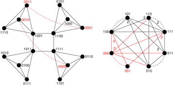
In lines 6 and 7, the entries of the vertex labels of $G_{a}$ are permuted according to a random permutation $\pi(\cdot)$. The construction of the hierarchy (lines 9 through 14) goes hand in hand with label swapping (lines 10-12) and label coarsening (in line 13). The function $\operatorname{contract}(\cdot,\cdot,\cdot)$ contracts any pair of vertices of $G_{a}^{i-1}$ whose labels agree on all but the last digit, thus generating $G_{a}^{i}$. The same function also cuts off the last digit of $l_{a}^{i-1}(v)$ for all $v\in V_{a}^{i-1}$, and creates the labeling $l_{a}^{i}(\cdot)$ for the next coarser level. Finally, $\operatorname{contract}(\cdot,\cdot,\cdot)$ builds the vector $\operatorname{parent}$ (for encoding the hierarchy of the vertices). In line 15, the call to $\operatorname{assemble}()$ derives a new labeling $l_{a}(\cdot)$ from the labelings $l_{a}^{i}(\cdot)$ on the levels $1\leq i\leq dim_{G_{a}}-1$ of a hierarchy (read more in Section 6.2). The permutation of $l_{a}$’s entries is undone in line 16, and $l_{a}(\cdot)$ is kept only if better than $l_{old}(\cdot)$, see lines 17 to 19. Figure 4 depicts a snapshot of TiMEr on a small instance.

Algorithm 1 Procedure TiMEr $(G_{a},G_{p},\mu(\cdot),N_{H})$ returns a bijection $l_{a}:V_{a}\mapsto\{0,1\}^{dim_{G_{a}}}$ with a low value of $\operatorname{Coco}(l_{a})$.

1:Find a labeling $l_{p}(\cdot)$ of $V_{p}$’s vertices, as described in Section 2

2:Using $\mu(\cdot)$, extend $l_{p}(\cdot)$ to a labeling $l_{a}(\cdot)$ of $V_{a}$’s vertices, as described in Section 4

3:for $N^{\prime}=1\dots,N_{H}$ do

4:    $l_{old}(\cdot)\leftarrow l_{a}(\cdot)$ $\triangleright$ just in case $l_{a}(\cdot)$ gets worse w. r. t. $\operatorname{Coco^{+}}(\cdot)$

5:    $\operatorname{parent}\leftarrow[]$ $\triangleright$ $\operatorname{parent}$ will encode the hierarchy of the vertices

6:    Pick a random permutation $\pi:\{1,\dots,dim_{G_{a}}\}\mapsto\{1,\dots,dim_{G_{a}}\}$

7:    $l_{a}(\cdot)\leftarrow\pi(l_{a}(\cdot))$

8:    $G_{a}^{1}\leftarrow G_{a}$, $l_{a}^{1}(\cdot)\leftarrow l_{a}(\cdot)$

9:    for $i=2,\dots,dim_{G_{a}}-1$ do

10:         for all $u,v\in G_{a}^{i-1}$ with $l_{a}^{i-1}(u)/2=l_{a}^{i-1}(v)/2$ do $\triangleright$ only least sig. digit differs

11:             Swap labels $l_{a}^{i-1}(u)$ and $l_{a}^{i-1}(v)$ if this decreases $\operatorname{Coco^{+}}(l_{a}^{i-1})$ on $G_{a}^{i-1}$.

12:         end for

13:         $(G_{a}^{i},l_{a}^{i},\operatorname{parent})\leftarrow\operatorname{contract}(G_{a}^{i-1},l_{a}^{i-1},\operatorname{parent})$

14:    end for

15:    $l_{a}(\cdot)\leftarrow\operatorname{assemble}(G_{a}^{1},\dots,G_{a}^{dim_{G}-1},l_{a}^{1},\dots,l_{a}^{dim_{G_{a}}-1},\operatorname{parent})$

16:    $l_{a}(\cdot)\leftarrow\pi^{-1}(l_{a}(\cdot))$

17:    if $\operatorname{Coco^{+}}(l_{a})>\operatorname{Coco^{+}}(l_{old})$ then

18:         $l_{a}(\cdot)\leftarrow l_{old}(\cdot)$

19:    end if

20:end for

21:return $l_{a}(\cdot)$

Algorithm 2 Function $\operatorname{assemble}(G_{a}^{1},\dots,G_{a}^{dim_{G}-1},l_{a}^{1},\dots,l_{a}^{dim_{G_{a}}-1},\operatorname{parent})$ returns a new labeling $l_{a}^{1}(\cdot)$ of the vertices of $G_{a}^{1}=G_{a}$ and thus a new labeling $l_{a}(\cdot)$ of $G_{a}$’s vertices.

1:for all $v_{1}\in V_{a}^{1}$ do

2:    $l_{a}^{1}(v_{1})\leftarrow l_{a}^{1}(v_{1})\operatorname{mod}2$ $\triangleright$ Write least significant digit

3:    $\operatorname{oldParent}\leftarrow v_{1}$

4:    $i\leftarrow 1$

5:    while $i<dim_{G_{a}^{1}}$ do $\triangleright$ Write digits $2,\dots,\dim_{G_{1}}-1$

6:         $\operatorname{newParent}\leftarrow\operatorname{parent}(\operatorname{oldParent})$

7:         $i\leftarrow i+1$

8:         $\operatorname{newParentLabel}\leftarrow l_{a}^{i}(\operatorname{newParent})$

9:         $\operatorname{prefLabel}\leftarrow l_{a}^{1}(v_{1})+(\operatorname{newParentLabel}\ll(i-1))$ $\triangleright$ Preferred $i$ least sig. digits

10:         if $\exists~{}w\in V_{1}$ with $l_{a}^{1}(w)\operatorname{mod}2^{i}=\operatorname{prefLabel}$ then $\triangleright$ Part of existing label?

11:             $l_{a}^{1}(v_{1})\leftarrow l_{a}^{1}(v_{1})+((\operatorname{newParentLabel}\operatorname{mod}2)\ll(i-1))$ $\triangleright$ Write preferred digit

12:         else

13:             $l_{a}^{1}(v_{1})\leftarrow l_{a}^{1}(v_{1})+((1-(\operatorname{newParentLabel}\operatorname{mod}2))\ll(i-1))$ $\triangleright$ Write other digit

14:         end if

15:         $\operatorname{oldParent}\leftarrow\operatorname{newParent}$

16:    end while

17:    if $l_{a}^{1}(v_{1})\geq 1\ll(dim_{G_{1}}-1)$ then

18:         $l_{a}^{1}(v_{1})\leftarrow l_{a}^{1}(v_{1})+(1\ll(dim_{G_{1}}-1))$ $\triangleright$ Write most significant digit

19:    end if

20:end for

21:return $l_{a}^{1}(\cdot)$

6.2. Function $\operatorname{assemble}()$

Function $\operatorname{assemble}()$ (Algorithm 2) in line 15 of TiMEr turns the hierarchy of graphs $G_{a}^{i}$ into a new labeling $l_{a}(\cdot)$ for $G_{a}$, digit by digit, using labels $l_{a}^{i}(\cdot)$ (in Algorithm 2, “$\ll i$” denotes a left shift by $i$ digits). The least and the most significant digit of any $l_{a}^{1}(v_{1})$ are inherited from $l_{a}(\cdot)$ (line 7 of Algorithm 1) and do not change (lines 2, 17 and 18). The remaining digits are set in the loop from line 5 to 16. Whenever possible, digit $i$ of $l_{a}^{1}(v_{1})$ is set to the last digit of the parent of $v_{1}$ (= preferred digit) on level $i$, see lines 9, 11. This might, however, lead to a label that is not in $l_{a}^{1}(V_{a}^{1})$ any more, which would change the set of labels and may violate the balance constraint coming from $\mu(\cdot)$. To avoid such balance problems, we take the last digit of $l_{a}^{i}(v_{a})$ if possible (in lines 9-11) or, if not, we switch to the (old) inverted digit, see line 13. Since $G_{a}^{1}=G_{a}$, new $l_{a}^{1}(\cdot)$ on $G_{a}^{1}$ can be taken as new $l_{a}(\cdot)$ on $G_{a}$, see line 18 in Algorithm 1.

6.3. Running time analysis

The expected asymptotic running time of function $\operatorname{assemble}()$ is $\mathcal{O}(|V_{a}|\cdot dim_{V_{a}})$. Here, “expected” is due to the condition in line 10 that is checked in expected constant time. (We use a hashing-based C++ std::unordered_map to find a vertex with a certain label. A plain array would be too large for large grids and tori, especially if the blocks are large, too.) For Algorithm 1, the expected running time is dominated by the loop between lines 9 and 14. The loop between lines 10 and 12 takes amortized expected time $\mathcal{O}(|E_{a}|)$ (“expected”, because we have to go from the labels to the vertices and “amortized”, because we have to check the neighborhoods of all $u,v$). The contraction in line 13 takes time $\mathcal{O}(|E_{a}|)$, too. Thus, the loop between lines 9 and 14 takes time $\mathcal{O}(|E_{a}|dim_{G_{a}})$. In total, the expected running time of Algorithm 1 is $\mathcal{O}(N_{H}~{}|E_{a}|~{}dim_{G_{a}})$.

An effective first step toward a parallel version of our algorithm would be simple loop parallelization in lines 10-12 of Algorithm 1. To avoid stale data, label accesses need to be coordinated.

7. Experiments

7.1. Description of experiments

In this section we specify our test instances, our experimental setup and the way we evaluate the computed mappings.

The application graphs are the 15 complex networks used by Safro et al. (Safro et al., 2012) for partitioning experiments and in (Glantz et al., 2015) for mapping experiments, see Table 1. Regarding the processor graphs, we follow loosely current architectural trends. Several leading supercomputers have a torus architecture (Deveci et al., 2015), and grids (= meshes) experience rising importance in emerging multicore chips (Clauss et al., 2011). As processor graphs $G_{p}=(V_{p},E_{p})$ we therefore use a 2DGrid($16\times 16$), a 3DGrid($8\times 8\times 8$), a 2DTorus($16\times 16$), a 3DTorus($8\times 8\times 8$) and, for more theoretical reasons, an $8$-dimensional hypercube. In our experiments, we set the number of hierarchies ($N_{H}$) for TiMEr to 50 and whenever is needed for partitioning/mapping with state-of-the-art tools, the load imbalance is set to 3%. All computations are based on sequential C++ code. Each experiment is executed on a node with two Intel XeonE5-2680 processors (Sandy Bridge) at 2.7 GHz equipped with 32 RAM and 8 cores per processor.

Table 1. Complex networks used for benchmarking.

Name	#vertices	#edges	Type
p2p-Gnutella	6 405	29 215	file-sharing network
PGPgiantcompo	10 680	24 316	largest connected component in network of PGP users
email-EuAll	16 805	60 260	network of connections via email
as-22july06	22 963	48 436	network of internet routers
soc-Slashdot0902	28 550	379 445	news network
loc-brightkite_edges	56 739	212 945	location-based friendship network
loc-gowalla_edges	196 591	950 327	location-based friendship network
citationCiteseer	268 495	1 156 647	citation network
coAuthorsCiteseer	227 320	814 134	citation network
wiki-Talk	232 314	1 458 806	network of user interactions through edits
coAuthorsDBLP	299 067	977 676	citation network
web-Google	356 648	2 093 324	hyperlink network of web pages
coPapersCiteseer	434 102	16 036 720	citation network
coPapersDBLP	540 486	15 245 729	citation network
as-skitter	554 930	5 797 663	network of internet service providers

Baselines.

For the evaluation, we use four different experimental cases ($\mathtt{c1}$ to $\mathtt{c4}$), each of which assumes a different initial mapping $\mu_{1}(\cdot)$ as an input to TiMEr (Algorithm 1). The different cases shall measure the improvement by TiMEr compared to different standalone mapping algorithms. In the following, we describe how we obtain the initial mappings $\mu_{1}(\cdot)$ for each case separately.

In $\mathtt{c1}$ we compare the improvement of TiMEr on an initial mapping produced by Scotch. For that, we use the generic mapping routine of Scotch with default parameters. It returns a mapping $\mu_{1}(\cdot)$ of a given graph using a dual recursive bipartitioning algorithm.

In $\mathtt{c2}$ we use the Identity mapping that maps block $i$ of the application graph (or vertex $i$ of the communication graph $G_{c}$) to node $i$ of the processor graph $G_{p}$, $1\leq i\leq|G_{c}|=|G_{p}|$. Identity receives its solution from the initial partition computed with KaHIP. This approach benefits from spatial locality in the partitions, so that Identity often yields surprisingly good solutions (Glantz et al., 2015).

In $\mathtt{c3}$ we use a mapping algorithm named GreedyAllC that has been previously proposed by a subset of the authors (implemented on top of KaHIP). GreedyAllC is an improvement of a previous greedy algorithm (Brandfass et al., 2013) and is the best performing algorithm in (Glantz et al., 2015). It builds on the idea of increasing a mapping by successively adding assignments $v_{c}\rightarrow v_{p}$ such that (a) $v_{c}\in G_{c}$ has maximal communication volume with one or all of the already mapped vertices of $G_{c}$ and (b) $v_{p}\in G_{p}$ has minimal distance to one or all of the already mapped vertices of $G_{p}$.

Finally, we compare against LibTopoMap (Hoefler and Snir, 2011), a state-of-the-art mapping tool that includes multiple mapping algorithm. More precisely we use the algorithm whose general idea follows the construct method, in (Brandfass et al., 2013) . Subset of the authors has previous implemented the above algorithm on top of the KaHIP tool (named GreedyMin). As a result, and in order to accommodate comparisons with $\mathtt{c2}$, $\mathtt{c3}$ GreedyMin is used as the mapping algorithm for the experimental case $\mathtt{c4}$.

Labeling.

Once the initial mappings $\mu_{1}(\cdot)$ are calculated, we need to perform two more steps in order to get an initial labeling $l_{a}(\cdot)$:

1. We compute a labeling $l_{p}~{}:~{}V_{p}\mapsto\{0,1\}^{dim_{G_{p}}}$, where $l_{p}(\cdot)$ and $dim_{G_{p}}$ fulfill the conditions in Definition 2.2. In particular, $d_{G_{p}}(u_{p},v_{p})=d_{h}(l_{p}(u_{p}),l_{p}(v_{p}))$ for all $u_{p},v_{p}\in V_{p}$, where $d_{h}(\cdot,\cdot)$ denotes the Hamming distance. Due to the sparsity of our processor graphs $G_{p}$ (grids, tori, hypercubes), we use the method outlined in Section 3.

2. We extend the labels of $G_{p}$’s vertices to labels of $G_{a}$’s vertices as described in Section 4.

Then, for each experimental case, TiMEr is given the initial mapping $\mu_{1}(\cdot)$ and it generates a new mapping $\mu_{2}(\cdot)$. Here, we compare the quality of mapping $\mu_{2}(\cdot)$ to $\mu_{1}(\cdot)$ in terms of our main objective function $\operatorname{Coco}(\cdot)$, but we also provide results for the edgecut metric and for the running times.

Metrics and parameters.

Since Scotch, KaHIP and TiMEr have randomized components, we run each experiment 5 times. Over such a set of 5 repeated experiments we compute the minimum, the arithmetic mean and the maximum of TiMEr’s running time ($T$), edge cut ($Cut$) and communication costs $\operatorname{Coco}(\cdot)$ ($Co$). Thus we arrive at the values $T_{min}$, $T_{mean},\dots,Co_{max}$ (9 values for each combination of $G_{a}$, $G_{p}$, for each experimental case $\mathtt{c1}$ to $\mathtt{c4}$). Each of these values is then divided by the min, mean, and max value before the improvements by TiMEr, except the running time of TiMEr, which is divided by the partitioning time of KaHIP for $\mathtt{c2}$,$\mathtt{c3}$,$\mathtt{c4}$ and by the mapping time of Scotch for $\mathtt{c1}$. Thus, we arrive at 9 quotients $qT_{min},\dots,qCo_{max}$. Except for the terms involving running times, a quotient smaller than one means that TiMEr was successful. Next we form the geometric means of the 9 quotients over the application graphs of Table 1. Thus we arrive at 9 values $qT^{gm}_{min},\dots,qCo^{gm}_{min}$ for any combination of $G_{p}$ and any experimental case. Additionally, we calculate the geometric standard deviation as an indicator of the variance over the normalized results of the application graphs.

7.2. Experimental Results

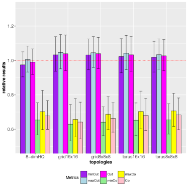
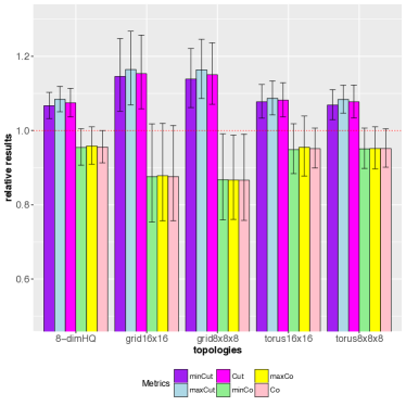
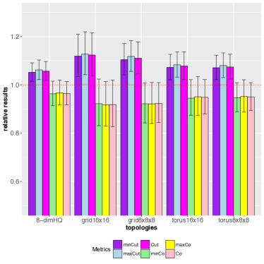
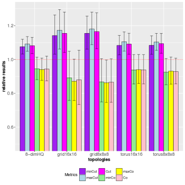
The detailed experimental results regarding quality metrics are displayed in Figures 5a through 5d (one for each experimental case), while the running time results are given in Table 2. Here is our summary and interpretation:

(a)

(b)

(c)

(d)

Figure 5. Quality results ($Co$ and $Cut$) for experimental case (a) $\mathtt{c1}$ (initial mapping with Scotch), (b) $\mathtt{c2}$ (initial mapping with Identity), (c) $\mathtt{c3}$ ((initial mapping with GreedyAllC)), and (d) $\mathtt{c4}$ (initial mapping with GreedyMin).

Table 2. Running time results of each experimental case. For $\mathtt{c1}$ results are relative to Scotch’s mapping time, while for $\mathtt{c2}$, $\mathtt{c3}$, $\mathtt{c4}$, results are relative to partitioning time with KaHIP (original values in Appendix A.1, Table 3)

	Scotch ($\mathtt{c1}$)			Identity ($\mathtt{c2}$)			GreedyAllC ($\mathtt{c3}$)			GreedyMin ($\mathtt{c4}$)
	$qT^{gm}_{min}$	$qT^{gm}_{mean}$	$qT^{gm}_{max}$	$qT^{gm}_{min}$	$qT^{gm}_{mean}$	$qT^{gm}_{max}$	$qT^{gm}_{min}$	$qT^{gm}_{mean}$	$qT^{gm}_{max}$	$qT^{gm}_{min}$	$qT^{gm}_{mean}$	$qT^{gm}_{max}$
$16\times 16$ grid	30.2780	29.8388	31.8387	0.95310	1.00480	1.05286	0.97916	1.01791	1.05075	0.95448	1.00681	1.05500
$8\times 8\times 8$ grid	18.0226	18.0484	19.5701	0.47495	0.49364	0.51333	0.47525	0.49427	0.51606	0.48712	0.50654	0.52698
$16\times 16$ torus	21.1373	21.2507	22.5322	0.61627	0.64089	0.66334	0.61743	0.63765	0.66042	0.64834	0.66524	0.68270
$8\times 8\times 8$ torus	13.8136	14.0924	14.3866	0.33254	0.34167	0.35008	0.32952	0.33885	0.34855	0.33412	0.34493	0.35744
$8$-dim HQ	11.2948	11.4237	11.5842	0.36821	0.37977	0.38916	0.36631	0.37246	0.38005	0.37254	0.38093	0.39196

• When looking at the running times for the experimental cases $\mathtt{c2}$ to $\mathtt{c4}$(in Table 2), we see that the running time results of TiMEr are on the same order of magnitude as partitioning with KaHIP; more precisely, TiMEr is on average 42% faster. Thus, inserting TiMEr into the partitioning/mapping pipeline of KaHIP would not increase the overall running time significantly.

  The comparison in case $\mathtt{c1}$ needs to be different. Here the initial mapping is produced by Scotch’s mapping routine (using partitioning internally), so that the relative timing results of TiMEr are divided by Scotch’s mapping time. Scotch is much faster (on average $19$x), but its solution quality is also not good (see $Co$ metric in Figure 5a). In informal experiments, we observed that only ten hierarchies (parameter $N_{h}$) are sufficient for TiMEr to improve the communication costs significantly compared to Scotch– with a much lower running time penalty than the one reported here. Finally, recall that parallelization could reduce the running time of TiMEr.

• Processor graphs do have an influence on running times. The processor graphs, from top to bottom in Table 2, have 30, 21, 32, 24 and 8 convex cuts, respectively. Thus, if we keep grids and tori apart, we can say that the time quotients increase with the number of convex cuts. Recall that the number of convex cuts equals the length of the labels of $V_{p}$. Moreover, the length of the extension of $V_{p}$’s labels to those of $V_{a}$ depends also on the processor graph, because a higher number of PEs (number of blocks) yields fewer elements per block. However, this influence on the length of the labels is small (increase of $1$ in case of $|V_{p}|=256$ compared to $|V_{p}|=512$). Thus it is basically the length of $V_{a}$’s labels that determines the time quotients. For the experimental cases $\mathtt{c2}$ to $\mathtt{c4}$, this observation is in line with the fact that KaHIP takes longer for higher values of $|V_{p}|$ (see Table 3 in Appendix A.1).

• TiMEr successfully reduces communication costs in a range from 6% to 34% over the different experimental cases (see $minCo,Co$ and $maxCo$ values in Figure 7.2). It does so at the expense of the edge cut metric with an average increase between 2% to 11% depending on the experimental case. Note that for case $\mathtt{c1}$ the edge cut increase is minimum (Figure 5a). Moreover, for cases $\mathtt{c2}$ to $\mathtt{c4}$ this increase is not surprising due to the different objectives of the graph partitioner (KaHIP) and TiMEr. On grids and tori, the reduction of communication cost, as measured by $\operatorname{Coco}(\cdot)$, is respectively 18% and 13% (on average, over all experimental cases).

  The better the connectivity of $G_{p}$, the harder it gets to improve $\operatorname{Coco}(\cdot)$ (results are poorest on the hypercube). (Note that $q_{min}$ values can be larger than $q_{mean}$ and $q_{max}$ values due to the evaluation process described in Section 7.1.)

  We observed before (Glantz et al., 2015) that GreedyAllC performs better on tori than on grids; this is probably due to GreedyAllC “invading” the communication graph and the processor graph. The resulting problem is that it may paint itself into a corner of the processor graph (if it has corners, like a grid). Thus, it is not surprising that for $\mathtt{c2}$ the improvement w. r. t. $\operatorname{Coco}(\cdot)$ obtained by TiMEr is greater for grids than for tori. Likewise, we observe that TiMEr is able to decrease the communication costs significantly for $\mathtt{c1}$ (even more than in the other cases). Apparently, the generic nature of Scotch’s mapping approach leaves room for such an improvement.

8. Conclusions

We have presented a new method, TiMEr, to enhance mappings of computational tasks to PEs. TiMEr can be applied whenever the processor graph $G_{p}$ is a partial cube. Exploiting this property, we supply the vertices of the application graph with labels that encode the current mapping and facilitate a straightforward assessment of any gains/losses of local search moves. By doing so, we are able to improve initial mappings using a multi-hierarchical search method.

Permuting the entries of the vertex labels in the application graph gives rise to a plethora of very diverse hierarchies. These hierarchies do not reflect the connectivity of the application graph $G_{a}$, but correspond to recursive bipartitions of $G_{a}$, which, in turn, are extensions of “natural” recursive bipartitions of $G_{p}$. This property of TiMEr suggests to use TiMEr as a complementary tool to enhance state-of-the-art methods for partitioning and mapping.

In our experiments we were able to improve state-of-the-art mappings of complex networks to different architectures by about $6\%$ to $34\%$ in terms of $\operatorname{Coco}$. More precisely, for grids we obtained, on average, an improvement of 18% and for tori an improvement of 13% over the communication costs of the initial mappings.

The novelty of TiMEr consists in the way it harnesses the fact that many processor graphs are partial cubes: the local search method itself is standard and simple. We assume that further improvements over state-of the art mappings can be achieved by replacing the simple local search by a more sophisticated method.

Appendix A Appendix

A.1. Additional experimental results

Table 3. Running times in seconds for KaHIP to partition the complex networks in Table 1 into $|V_{p}|=256$ and $|V_{p}|=512$ parts, respectively. These partitions are used to construct the starting solutions for the mapping algorithms for cases $\mathtt{c2}$ to $\mathtt{c4}$.

Name	$|V_{p}|=256$	$|V_{p}|=512$
PGPgiantcompo	1.457	2.297
as-22july06	11.179	13.559
as-skitter	1439.316	2557.827
citationCiteseer	217.951	367.716
coAuthorsCiteseer	58.120	69.162
coAuthorsDBLP	157.871	233.000
coPapersCiteseer	780.491	841.656
coPapersDBLP	1517.283	2377.680
email-EuAll	22.919	17.459
loc-brightkite_edges	113.720	155.384
loc-gowalla_edges	461.583	1174.742
p2p-Gnutella04	16.377	17.400
soc-Slashdot0902	887.896	1671.585
web-Google	128.843	130.986
wiki-Talk	1657.273	4044.640
Arithmetic mean	498.152	911.673
Geometric mean	142.714	204.697

References

- (1)
- Aubanel (2009) Eric Aubanel. 2009. Resource-Aware Load Balancing of Parallel Applications. In Handbook of Research on Grid Technologies and Utility Computing: Concepts for Managing Large-Scale Applications, Emmanuel Udoh and Frank Zhigang Wang (Eds.). Information Science Reference - Imprint of: IGI Publishing, 12–21.
- Bichot and Siarry (2011) C. Bichot and P. Siarry (Eds.). 2011. Graph Partitioning. Wiley.
- Brandfass et al. (2013) B. Brandfass, T. Alrutz, and T. Gerhold. 2013. Rank Reordering for MPI Communication Optimization. Computers & Fluids 80, 0 (2013), 372 – 380. https://doi.org/10.1016/j.compfluid.2012.01.019
- Buluç et al. (2016) Aydin Buluç, Henning Meyerhenke, Ilya Safro, Peter Sanders, and Christian Schulz. 2016. Recent Advances in Graph Partitioning. In Algorithm Engineering - Selected Results and Surveys, Lasse Kliemann and Peter Sanders (Eds.). Lecture Notes in Computer Science, Vol. 9220. 117–158.
- Chan et al. (2012) Siew Yin Chan, Teck Chaw Ling, and Eric Aubanel. 2012. The Impact of Heterogeneous Multi-Core Clusters on Graph Partitioning: An Empirical Study. Cluster Computing 15, 3 (2012), 281–302.
- Chevalier and Safro (2009) Cédric Chevalier and Ilya Safro. 2009. Comparison of Coarsening Schemes for Multilevel Graph Partitioning. In Learning and Intelligent Optimization, Third International Conference, LION 3, Trento, Italy, January 14-18, 2009. Selected Papers (Lecture Notes in Computer Science), Thomas Stützle (Ed.), Vol. 5851. Springer, 191–205.
- Clauss et al. (2011) C. Clauss, S. Lankes, P. Reble, and T. Bemmerl. 2011. Evaluation and improvements of programming models for the Intel SCC many-core processor. In 2011 International Conference on High Performance Computing Simulation. 525–532.
- Deveci et al. (2015) M. Deveci, K. Kaya, B. Uçar, and U. V. Catalyurek. 2015. Fast and High Quality Topology-Aware Task Mapping. In 2015 IEEE International Parallel and Distributed Processing Symposium. 197–206.
- Eppstein (2011) D. Eppstein. 2011. Recognizing Partial Cubes in Quadratic Time. J. Graph Algorithms Appl. 15, 2 (2011), 269–293.
- Garey and Johnson (1979) Michael R. Garey and David S. Johnson. 1979. Computers and Intractability: A Guide to the Theory of NP-Completeness. W. H. Freeman & Co.
- Glantz et al. (2015) R. Glantz, H. Meyerhenke, and A. Noe. 2015. Algorithms for Mapping Parallel Processes onto Grid and Torus Architectures. In 23rd Euromicro International Conference on Parallel, Distributed and Network-Based Processing, PDP 2015, Turku, Finland. 236–243.
- Hoefler and Snir (2011) T. Hoefler and M. Snir. 2011. Generic Topology Mapping Strategies for Large-scale Parallel Architectures. In ACM International Conference on Supercomputing (ICS’11). ACM, 75–85.
- Imrich (1993) W. Imrich. 1993. A simple O(mn) algorithm for recognizing Hamming graphs. Bull. Inst. Comb. Appl (1993), 45–56.
- Jeannot et al. (2013) E. Jeannot, G. Mercier, and F. Tessier. 2013. Process Placement in Multicore Clusters: Algorithmic Issues and Practical Techniques. IEEE Transactions on Parallel and Distributed Systems PP, 99 (2013), 1–1. https://doi.org/10.1109/TPDS.2013.104
- Karypis and Kumar (1998) G. Karypis and V. Kumar. 1998. A Fast and High Quality Multilevel Scheme for Partitioning Irregular Graphs. SIAM J. Sci. Comput. 20, 1 (1998), 359–392.
- Kernighan and Lin (1970) B. W. Kernighan and S. Lin. 1970. An efficient heuristic procedure for partitioning graphs. Bell Systems Technical Journal 49 (1970), 291–307.
- Kim and Lai (1991) Young Man Kim and Ten-Hwang Lai. 1991. The Complexity of Congestion-1 Embedding in a Hypercube. Journal of Algorithms 12, 2 (1991), 246 – 280. https://doi.org/10.1016/0196-6774(91)90004-I
- Kirmani et al. (2017) Shad Kirmani, JeongHyung Park, and Padma Raghavan. 2017. An embedded sectioning scheme for multiprocessor topology-aware mapping of irregular applications. IJHPCA 31, 1 (2017), 91–103. https://doi.org/10.1177/1094342015597082
- Meyerhenke et al. (2009) Henning Meyerhenke, Burkhard Monien, and Thomas Sauerwald. 2009. A New Diffusion-based Multilevel Algorithm for Computing Graph Partitions. J. Parallel and Distributed Computing 69, 9 (2009), 750–761. https://doi.org/DOI:10.1016/j.jpdc.2009.04.005
- Osipov and Sanders (2010) Vitaly Osipov and Peter Sanders. 2010. n-Level Graph Partitioning. In Algorithms - ESA 2010, 18th Annual European Symposium, Liverpool, UK, September 6-8, 2010. Proceedings, Part I (Lecture Notes in Computer Science), Mark de Berg and Ulrich Meyer (Eds.), Vol. 6346. Springer, 278–289.
- Ovchinnikov (2008) S. Ovchinnikov. 2008. Partial cubes: Structures, characterizations, and constructions. Discrete Mathematics 308 (2008), 5597–5621.
- Pellegrini (1994) François Pellegrini. 1994. Static Mapping by Dual Recursive Bipartitioning of Process and Architecture Graphs. In Scalable High-Performance Computing Conference (SHPCC). IEEE, 486–493.
- Pellegrini (2007) François Pellegrini. 2007. Scotch and libScotch 5.0 User’s Guide. Technical Report. LaBRI, Université Bordeaux I.
- Pellegrini (2011) François Pellegrini. 2011. Static Mapping of Process Graphs. In Graph Partitioning, Charles-Edmond Bichot and Patrick Siarry (Eds.). John Wiley & Sons, Chapter 5, 115–136.
- Que et al. (2015) Xinyu Que, Fabio Checconi, Fabrizio Petrini, and John A. Gunnels. 2015. Scalable Community Detection with the Louvain Algorithm. In 2015 IEEE International Parallel and Distributed Processing Symposium, IPDPS 2015, Hyderabad, India, May 25-29, 2015. IEEE Computer Society, 28–37.
- Safro et al. (2012) I. Safro, P. Sanders, and Ch. Schulz. 2012. Advanced Coarsening Schemes for Graph Partitioning. In Proc. 11th Int. Symp. on Experimental Algorithms. Springer, 369–380.
- Sanders and Schulz (2013a) P. Sanders and C. Schulz. 2013a. High Quality Graph Partitioning. In Proc. of the 10th DIMACS Impl. Challenge Workshop: Graph Partitioning and Graph Clustering. AMS, 1–17.
- Sanders and Schulz (2013b) Peter Sanders and Christian Schulz. 2013b. KaHIP v0.53 - Karlsruhe High Quality Partitioning - User Guide. CoRR abs/1311.1714 (2013).
- Schulz and Träff (2017) C. Schulz and J. L. Träff. 2017. Better Process Mapping and Sparse Quadratic Assignment. CoRR abs/1702.04164 (2017).
- Trobec and Kosec (2015) Roman Trobec and Gregor Kosec. 2015. Parallel Scientific Computing. Theory, Algorithms, and Applications of Mesh Based and Meshless Methods. Springer Intl. Publ. https://doi.org/10.1007/978-3-319-17073-2
- Ucar et al. (2006) Bora Ucar, Cevdet Aykanat, Kamer Kaya, and Murat Ikinci. 2006. Task Assignment in Heterogeneous Computing Systems. J. Parallel and Distrib. Comput. 66, 1 (2006), 32 – 46.
- Walshaw and Cross (2001) Chris Walshaw and Mark Cross. 2001. Multilevel Mesh Partitioning for Heterogeneous Communication Networks. Future Generation Comp. Syst. 17, 5 (2001), 601–623.
- Yu et al. (2006) Hao Yu, I-Hsin Chung, and Jose Moreira. 2006. Topology Mapping for Blue Gene/L Supercomputer. In Proceedings of the 2006 ACM/IEEE Conference on Supercomputing (SC ’06). ACM, New York, NY, USA.