.tifpng.pngconvert #1 \OutputFile \AppendGraphicsExtensions.tif
Primordial Black Holes from Inflation and Quantum Diffusion
M. Biagettia***m.biagetti@uva.nl, G. Franciolinib†††gabriele.franciolini@unige.ch, A. Kehagiasc‡‡‡kehagias@central.ntua.gr and A. Riottob§§§antonio.riotto@unige.ch
a Institute of Physics, Universiteit van Amsterdam, Science Park, 1098XH Amsterdam, The Netherlands
bDepartment of Theoretical Physics and Center for Astroparticle Physics (CAP)
24 quai E. Ansermet, CH-1211 Geneva 4, Switzerland
cPhysics Division, National Technical University of Athens, 15780 Zografou Campus, Athens, Greece
Abstract
Primordial black holes as dark matter may be generated in single-field models of inflation thanks to the enhancement at small scales of the comoving curvature perturbation.
This mechanism requires leaving the slow-roll phase to enter a non-attractor phase during which the inflaton travels across a plateau and its velocity drops down
exponentially. We argue that quantum diffusion has a significant impact on the primordial black hole mass fraction making the classical standard prediction not trustable.
I. Introduction
The interest in the physics of Primordial Black Holes (PBHs) and the possibility that they form all (or a fraction) of the dark matter in the universe has risen up [1, 2, 3, 4, 5, 6, 7, 8, 9, 10] again after the discovery of two black holes through the gravitational waves generated during their merging [11]. A standard mechanism to account for the generation of the PBHs is through the boost of the curvature perturbation at small scales [12, 13, 14]. Such an enhancement can occur either within single-field models of inflation, see Refs [15, 16, 17, 18, 19] for some recent literature, or through some spectator field [20, 21, 22, 23] which could be identified the Higgs of the Standard Model [24].
In order for this primordial mechanism to occur, one needs an enhancement of the power spectrum of the curvature perturbation from its value at large scales to on small scales. Subsequently, these large perturbations are communicated to radiation during the reheating process after inflation and they may give rise to PBHs upon horizon re-entry if they are sizeable enough. If we indicate by the comoving curvature power spectrum, a region of size the Hubble radius may collapse and form a PBH if the corresponding square root of the variance smoothed with a high-pass filter on the same length scale (comoving momenta larger than the inverse of the comoving Hubble) is larger than some critical value . Its exact value is sensitive to the equation of state upon horizon re-entry and it is about 0.086 for radiation [25]. However, larger values have been adopted in the literature [26, 27, 28]. We will later on use the common representative value .
Under the (strong) hypothesis that the curvature perturbation obeys a Gaussian statistics, the primordial mass fraction of the universe occupied by PBHs formed at the time of formation reads
| (1.1) |
It corresponds to a present dark matter abundance made of PBH of masses given by (neglecting accretion) [28]
| (1.2) |
where is a parameter accounting for the efficiency of the collapse and is the effective number of degrees of freedom. Imposing PBHs to be the dark matter, values require larger values of and therefore to be conservative we impose [28]
| (1.3) |
For a mass of the order of we find [28]
| (1.4) |
Now, in single-field models of inflation the power spectrum of the comoving curvature perturbation is given by (we set the Planckian mass equal to one from now on) [29]
| (1.5) |
where is the number of e-folds, the prime denotes differentiation with respect to , and is the Hubble rate. The generation of PBHs requires the jumping within a few e-folds of the value of the power spectrum of about seven orders of magnitude from its value on CMB scales. Without even specifying the single-field model of inflation, one may conclude that there must be a violation of the slow-roll condition as must change rapidly with time. This may happen when the inflaton field goes through a so-called non-attractor phase (dubbed also ultra-slow-roll) [30, 31, 32, 33, 34, 35, 36, 37, 38, 39] in the scalar potential, thus producing a sizeable resonance in the power spectrum of the curvature perturbation.
When the inflaton experiences a plateau in its potential, since must be extremely small, a short non-attractor period is achieved during which the equation of motion of the inflaton background reduces to
| (1.6) |
where ,ϕ denotes differentiation with respect to the inflaton field with potential . The comoving curvature perturbation increases, due to its decaying mode which in fact is growing, as
| (1.7) |
It is this exponential growth which helps obtaining large fluctuations in the curvature perturbation and the formation of PBHs upon horizon re-entry during the radiation phase. This is also the reason why the power spectrum should be quoted at the end of inflation and not, as usually done in slow-roll, at Hubble crossing: its value at the instant of Hubble crossing differs by a significant factor from the asymptotic value at late times. Not respecting these rules might lead to an incorrect estimate of the power spectrum and consequently of the PBH abundance at formation, see e.g. Ref. [40] and the subsequent discussions in Refs. [36, 28].
Putting aside the strong sensitivity of the PBH mass fraction at formation to possible non-Gaussianities [14, 41, 42, 43, 44, 45, 46, 47, 48, 49, 50] which is common to all mechanisms giving rise to PBHs through sizeable perturbations (we will however devote Appendix C for some considerations about non-Gaussianity where we will show that the formalism [51] can help in assessing the role of non-Gaussianity for those perturbations generated during the non-attractor phase) in this paper we are interested in another issue, the role of quantum diffusion. One might be reasonably suspicious that during the non-attractor phase the quantum diffusion becomes relevant [49]. The reason is the following. The stochastic equation of motion for the classical inflaton field takes into account that each Hubble time the inflaton field receives kicks of the order of [52]
| (1.8) |
where is a Gaussian random noise with
| (1.9) |
During the non-attractor phase, needs to be tiny enough to allow to promptly decrease thus violating slow-roll. For the same reason, one needs to make sure that quantum jumps are not significant in this case. One could try to impose the condition
| (1.10) |
to be satisfied during the non-attractor phase. In slow-roll, the condition (1.10) could be exactly expressed in terms of the power spectrum and the latter would be required to be smaller than unity, thereby giving a direct constraint on a physical observable. However, during the non-attractor phase, the bound (1.10) is not directly expressed in terms of the power spectrum (1.5), making the comparison with physical observables more difficult. One might naively think that during the non-attractor phase the noise is not relevant if is larger than [17]. However, this is not correct for two reasons. First because, as we will see, the relevant noise to be evaluated is the one for the inflaton velocity. Secondly, and above all, because this is not the right criterion to evaluate the strong impact of quantum diffusion onto the PBH mass fraction.
We will first elaborate on the computation of the power spectrum during the non-attractor phase in order to understand some basic features of the power spectrum itself, e.g. its time evolution and the location of its peak. This will be useful for the considerations about the quantum diffusion. We will then use the so-called Kramers-Moyal equation [53] to assess the impact of quantum diffusion.
The Kramers-Moyal equation is the suitable starting point as it highlights the importance of the inflaton velocity and it is a generalisation of the Fokker-Planck equation. Indeed, in general the Kramers-Moyal equation contains an infinite number of derivatives with respect to the inflaton field after having integrated out the velocity, while the Fokker-Planck equation is a truncation of the Kramers-Moyal equation by retaining only two spatial derivatives of the inflaton field. This is not an irrelevant point: Pawula’s theorem [54] tells us that if we set to zero some coefficient of the higher derivative terms with respect to the inflaton field with , then all the coefficients of the higher derivatives are zero. It is therefore not consistent to keep some higher derivative term unless all of them are kept. This means that, whenever the Kramers-Moyal equation may not be solved exactly, a numerical approach is useful to solve it without applying an unjustified truncation.
We will present both analytical and numerical results to quantify the impact of quantum diffusion on the PBH abundance. In the simplest case of non-attractor phase with an approximately linear or quadratic potential, the system can be solved analytically. For a linear potential, the stochastic motion of the system is characterised by the fact that the variance of the velocity rapidly converges towards a stationary value. For a quadratic potential, the spread in the velocity varies with time, although slowly, away from the stationary point.
However, for more complicated situations, e.g. if during the non-attractor phase the inflaton goes through an inflection point, a numerical analysis is called for and we will show that the spread in the velocity grows with time. If this growth is too large, classicality as well as information on the PBH abundance is lost. We will propose two criteria to be respected in order to neglect the quantum diffusion and we will see that the curvature perturbation is severely constrained from above in order to avoid an undesirable spreading of the velocity wave packet. We will also argue that the capability of the standard (that is classical) calculation to predict the correct dark matter abundance in terms of PBH is severely challenged by the presence of quantum diffusion.
This paper is organised as follows. In section II we discuss the computation of the curvature perturbation during the non-attractor phase. We then start our study of the quantum diffusion, both analytically and numerically, in section III and IV respectively. In sections V and VI we offer two criteria to assess the importance of the diffusion. Finally, in section VII we offer our conclusions.
The paper contains several Appendices. Appendix A deals with the curvature perturbation, the Schwarzian derivative and the dual transformation; appendix B with the study of the evolution of the comoving curvature perturbation from the non-attractor phase back to the slow-roll phase; appendix C offers some consideration about non-Gaussianity.
II. The comoving curvature perturbation and the non-attractor phase
In this section we offer some considerations about the curvature perturbation generated thanks to the non-attractor phase. We start by some analytical considerations and then we will proceed with a more realistic example.
Non-attractor: some analytical considerations
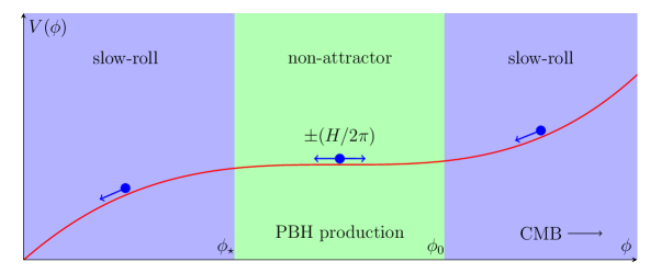
We are interested in the curvature perturbation for those modes leaving the Hubble radius deep in the non-attractor phase. We suppose that the non-attractor phase starts when the inflaton field acquires the value and ends when it becomes equal to . We also assume that the non-attractor phase is preceded and followed by slow-roll phases, see Fig. 1. During these phases passes from a tiny value (slow-roll) to 3 (non-attractor) back to small values (slow-roll).
To treat the problem analytically, we suppose that during the non-attractor phase we may Taylor expand the inflaton potential as
| (2.1) |
where is the slow-roll parameter. Of course, the potential during the non-attractor phase may be more complex, but its linearisation captures the main features.
Computing everything in terms of the number of e-folds and defining the beginning of the non-attractor phase with initial conditions and and setting , the solution of the equations of motion leads to
| (2.2) |
We see that if the inflaton field starts with a large velocity from the preceeding slow-roll phase, there is a period over which the velocity of the inflaton field decays exponentially. Depending on the duration of the non-attractor phase, the velocity may or may not attain its slow-roll asymptote given by . Indicating by the value of the velocity at the end of the non-attractor phase, the final value of the curvature perturbation at the end of the non-attractor phase is given by
| (2.3) |
The corresponding power spectrum is flat. This might come as a surprise as slow-roll is badly violated, but in fact its a direct consequence of the dual symmetry described in Ref. [55] (see also Refs. [56, 57, 58]). We elaborate extensively on this point in Appendix A. In a nutshell and alternatively, one can show it in the following way. Using the conformal time and setting , , where is the Hubble rate in conformal time, one can write the equation for the function as (cfr. Eq. (A.2))
| (2.4) |
where and are the slow-roll parameters defined in Eq. (Appendix A: the curvature perturbation, the Schwarzian derivative and the dual transformation) and is the scale factor. Since during the non-attractor phase , and the potential is very flat, the right-hand side of the previous equation is approximated on super-Hubble scales to and therefore . It provides the standard solution for the mode function of the curvature perturbation
| (2.5) |
This is the standard slow-roll solution with the crucial exception that the inflaton velocity changes rapidly with time. Notice also that the expression (2.3) can be extended at the end of inflation. This is possible if the transition from the non-attractor phase to the subsequent slow-roll phase (if any) is sudden, i.e. the velocity during the subsequent slow-roll phase is much bigger than . Under these circumstances, the power spectrum does not have time to change and remains indeed (2.3) till the end of inflation [39]. We give more details in Appendix B.
So far, we have discussed the perturbation associated to the modes which leave the Hubble radius deep in the non-attractor phase. However, the peak of the curvature perturbation is in fact reached for those modes which leave the Hubble radius during the sudden transition from the slow-roll phase into the non-attractor phase. During this transition the (would-be) slow-roll parameter jumps from a tiny value to 3.
To see what happens, we model the parameter as , where we have now turned again to conformal time . If so, and if we indicate by the slow-roll parameter during the slow-roll phase preceding the non-attractor phase and assume it to be constant in time, one has
| (2.6) |
and [39]
| (2.7) |
where we have taken into account that immediately after the beginning of the non-attractor phase the curvature perturbation increases as the inverse cubic power of the conformal time (cfr. Eq. (2.2)). Imposing continuity of the two functions together of their derivatives, one obtains a power spectrum at the end of inflation
| (2.8) |
The function is for , has a maximum of about 2.5 around and oscillates rapidly around 1 for . We can conclude that the power spectrum has the following shape: it increases, reaches a peak, and then decreases a bit till a plateau is encountered. This is in good agreement with what obtained, for instance, in Refs. [58, 57]. The amplitude of the peak is about 2.5 times larger than the plateau in correspondence of the modes which leave the Hubble radius during the non-attractor phase
| (2.9) |
Of course, given the assumption of sudden transition of from tiny values to around and having assumed constant, we expect this number to change by a factor depending upon the exact details. The linearisation of the potential is an approximation, but it captures the main features of the final result. For more complicated situations, for instance if during the non-attractor phase the inflation crosses an inflection point, one expects again a peak in the curvature perturbation for that mode leaving the Hubble radius at the sudden transition between the slow-roll and the non-attractor phase. However, one does not expect a significant plateau following the maximum as the non-attractor phase is typically very short. This also implies that the exact amplitude of the peak depends on the fine details of the transition.
An example: Starobinsky’s model.
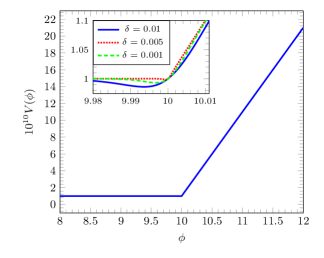
In order to assess the quality of our findings we can consider Starobinsky’s model [59] which is characterised by a potential with two linear regions
| (2.10) | ||||
| (2.11) |
where are the slow-roll parameter during the slow-roll phase and the non-attractor phase, respectively. In fact, to deal with the problem numerically we have parametrised the discontinuity in the potential as
| (2.12) |
where determines the size of the region in which the potential smoothly changes slope. If the potential during the non-attractor phase becomes exactly linear. We will comment on the effect of varying on the quantum diffusion in Sec. IV.
If , a prolonged non-attractor phase is obtained during which
| (2.13) |
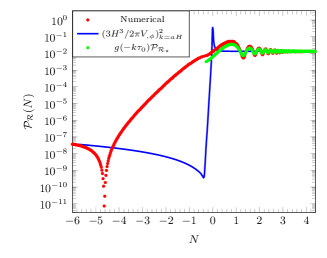
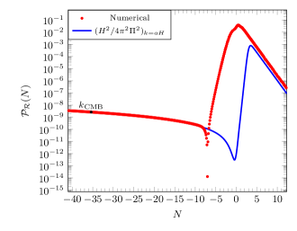
The inflaton velocity at the beginning of the non-attractor phase is , then it quickly decays reaching a maximum (recall velocities are negative) at and then it reaches the value . The corresponding power spectrum in Fig. 2 illustrates three relevant points: the fact that the power spectrum reaches a plateau and becomes scale-independent, the amplitude of the plateau is reproduced by the standard slow-roll formula (see Appendix A) and finally that the formula (Non-attractor: some analytical considerations) provides a good fit to the numerical result.
Non-attractor: more physical cases
We turn now the discussion to more physical cases discussed recently in the literature. First, we consider the model in Ref [18]. Leaving aside the details of the particular string model giving rise to it, the inflaton potential reads
| (2.14) |
where the parameters used in our analysis can be found in Tab. 1.
| 0.02 | 1 | 0.04 | 0 |
|---|
We have checked that they provide the correct CMB normalisation at large scales, as well as the correct spectral index and PBH abundance to match the dark matter abundance. The inflaton potential has an inflection point violating the slow-roll conditions, see Fig. 3, where the field is forced to enter a non-attractor phase which lasts a few e-folds and a boost in the curvature power spectrum is generated.
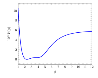

The solution to the Friedmann equations shows that the background evolution can be divided as follows. In a first stage the field experiences a slow-roll evolution compatible with the constraints on CMB scales. When the field approaches the local minimum, the fields enters a non-attractor phase where . After the following local maximum, the field exits the non-attractor phase leading to the end of the inflationary era.
We numerically solve the equation for the comoving curvature perturbation (cfr. Eq. (A.1)) starting from the usual Bunch-Davies vacuum in the asymptotic region . Fig. 4 shows the power spectrum and the behaviour of the different modes.
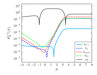
We have indicated by the mode leading to the largest amplitude and by the mode that leaves the Hubble radius at the transition point (approximately at in Fig 4). We have called and the wavenumbers respectively 0.1 and 10 times larger than . We have also plotted the power spectrum computed at Hubble crossing to show its inadequacy in reproducing the exact result which must be calculated at the end of the non-attractor phase. Notice also that the curvature perturbation grows until the end of the non-attractor phase, meaning that it takes advantage of the exponential decrease of the inflaton velocity until the end of the non-attractor phase, then it remains constant until the end of inflation. As we mentioned, this is because the transition back to the slow-roll phase is sudden and despite the fact that the parameter does not go back immediately to very small values [39]. As for the absolute amplitude of the perturbation at the peak, we cannot really make use of the formula (2.3) since when the mode leaves the Hubble radius both and change considerably. Numerically, we have estimated .
In the following we will also perform our analysis of the model in Ref. [19]. The inflaton potential
| (2.15) |
is characterised by a series of oscillations around the quadratic potential, the last of which is capable of generating an inflection point, tuned such that the power-spectrum is enhanced as previously described for model [18], see Fig. 5.
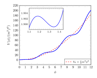

We have chosen to use the parameter set 1 in Ref. [19] for our analysis for sake of comparison. Also for this case we have numerically estimated . The models in Refs. [18, 19] are similar to those of other recent literature [15, 16, 17, 40] and we expect our analysis for the quantum diffusion to apply to those cases too.
III. The non-attractor phase and quantum diffusion
Let us now come back to the role of quantum diffusion. If too large, quantum diffusion causes a loss of information as the curvature perturbation may not be reconstructed any longer at late times in terms of classical trajectories [17]. Different scales mix and the corresponding amplitude will be left undetermined for an observer at late times. Since quantum diffusion becomes more and more relevant as the field slows down and consequently the power spectrum grows, this clearly creates an issue and one expects a upper bound on the curvature perturbation in order for the quantum diffusion to be irrelevant.
Since the power spectrum is fixed by the inverse of the velocity of the inflaton field at the end of the non-attractor phase, we expect that, if the spread of the distribution of velocities caused by the stochastic motion is too large, then along most of the trajectories the perturbation will be either too large or to too small to generate PBHs in the allowed range of masses. One has therefore to find the amount of dispersion undergone by the velocity of the inflaton field.
Let us also notice that the power spectrum is growing during the non-attractor phase after the corresponding wavelength leaves the Hubble radius and therefore the issue of the quantum diffusion becomes more relevant at the end of the non-attractor phase. We will therefore discuss the criterion at the end of such a phase, where one expects the strongest constraints.
The stochastic equation (1.8) can be written as an Ornstein-Uhlenbeck process
| (3.1) |
where is the diffusion coefficient. We may write the Kramers-Moyal (KM) equation for the corresponding probability as [53]
| (3.2) |
where
| (3.3) |
The initial condition for the probability can be taken to be
| (3.4) |
as we assume that during the preceding slow-roll phase the motion is purely along classical trajectories.
Generic potential
We re-write the KM equation as
The stationary solution for the operator is proportional to and we can generate a Hermitian operator
| (3.6) |
where
| (3.7) |
are the annihilation and creator operators with . To take advantage of this procedure, we also redefine the operator
| (3.8) |
where is an arbitrary constant
| (3.9) |
with . Now, the orthonormalised eigenfunctions of the operator , that is
| (3.10) |
are
| (3.11) |
Since the operator is of the form
| (3.12) |
or
| (3.13) |
we can expand the probability as [53]
| (3.14) |
so that the distribution in the inflaton field is only given by the first term of the expansion
| (3.15) |
where nevertheless the coefficients satisfy the so-called Brinkman’s hierarchy
| (3.16) |
and it is equivalent to the KM equation. This equation contains an infinite number of terms. For pedagogical purposes, let us truncate though the system by setting for , so that the Brinkman’s hierarchy reduces to
| (3.17) |
For a large friction term one can neglect the term , and we could eliminate in favour of . Setting , we find
| (3.18) |
which is the standard Fokker-Planck equation. Had not we dropped the term , we could have eliminated and get the equation for
| (3.19) |
which is Brinkman’s equation. Retaining the coefficients with will introduce spatial derivatives higher than two. We find here what we mentioned in the introduction, that the KM contains an infinite tower of spatial derivatives of the effective probability of the inflaton field and, due to Pawula’s theorem, it is not consistent to drop derivatives higher than two. In this sense, the Fokker-Planck equation is not the correct starting point.
In the case of a linear potential the operators and commute, while for a quadratic potential their commutator is a constant and the analysis is made it easier. We will consider these cases next.
Linear potential
We consider first the linear potential (2.1) as a prototype. In such a case, the KM equation has an exact solution [53]
where
| (3.21) |
and
| (3.22) |
At times , the probability becomes
| (3.23) |
Integrating over we obtain
| (3.24) |
and
| (3.25) |
Conversely, integrating over the scalar field , one obtains
| (3.26) |
and
| (3.27) |
We conclude that when the average velocity of the inflaton field decays exponentially, its variance reaches quickly an asymptotic and stationary value given by Eq. (3.27). There is an alternative way to obtain the same result. From the KM equation, we may derive the following set of equations
| (3.28) |
At times larger than a few Hubble times, the correlators involving decay promptly to their equilibrium values resulting in
| (3.29) |
Linear plus quadratic potential
Our considerations can be extended beyond the linear order in the potential. Let us expand the potential including the quadratic order
| (3.30) |
where parametrises the second derivative of the potential. The equation of motion leads to a classical value
| (3.31) |
In particular, if one has a potential where corresponds to a minimum and only the quadratic piece is there in the Taylor expansion one finds
| (3.32) |
In order to simplify the problem, we notice that in the stochastic equation of motion of the inflaton field
| (3.33) |
one can shift the field by an amount and by an amount in order to get rid of the constant force. The problem reduces for this shifted field to the following set of equations (we do not redefine the fields to avoid cluttering notation)
| (3.34) |
The solution of these equations is again given in Eq. (Linear potential). This time however
| (3.37) |
Also, by defining
| (3.38) |
one obtains [53]
| (3.39) |
or
| (3.40) |
At large times and for small they reduce to
| (3.41) |
For , i.e. for a harmonically bound state, in the large time limit one obtains a stationary solution. However, for , i.e. for an inverted parabolic potential, the force felt by the inflaton is repulsive. In both cases, the width of the distribution of the inflaton velocities obtained integrating out over all possible values of the inflaton field reads
| (3.42) |
In the model of Ref. [18, 19] the plateau is in fact a region around an inflection point between a minimum and a maximum so that changes sign from positive to negative (if the minimum is encountered first). Being the dynamics more complex than what described above, we should expect deviations of order unity from our estimate.
IV. Numerical analysis of quantum diffusion
In this section we present the numerical studies we performed in order to check the validity of our analytical findings. We have numerically solved the system (III. The non-attractor phase and quantum diffusion) with the available Mathematica routines for the solution of stochastic differential equations. We focus only on the inflaton velocity since the perturbations are sensitive to it. The spread in the inflaton field, which acquires typically Planckian values (at least in the vast majority of the literature) is irrelevant. At any rate, we have numerically checked that our numerical results coincide with this statement. We were able to test the robustness of our numerical implementation for the case of the linear potential, for which we have the analytical solution, Eq. (Linear potential).
Linear potential and Starobinsky’s model
We start by checking the solution of the KM equation in the case of a linear potential. Since we are interested in the dispersion of around its classical value, we recover numerically its variance among many realizations of the stochastic evolution.
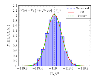
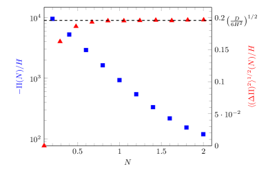
In Fig. 6, one can see the comparison between the prediction (3.27) and the numerical results. The numerical results, obtained integrating over the inflaton field positions (whose spread is however tiny with respect to the average classical position), fully reproduce the analytical results (to the extent that the red line of the fit and the green one representing the theory overlap perfectly).
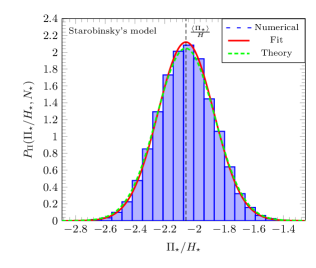
We have also repeated our analysis for Starobinsky’s model [59] we have introduced in section II. The results are in Fig. 7 which show that the spread of the velocity approaches . For smaller values of , the agreement with the linear potential result would be extended to the whole non-attractor phase, but the choice of is limited by numerical precision.
More physical cases
Having established that the numerical and analytical results agree for the simple case of the linear potential, we now turn our attention to more realistic cases discussed in the literature. As a representative example of the models in the literature, we consider the ones described in Ref. [18] and [19] already introduced in Sec. II. We solve numerically the stochastic equations (III. The non-attractor phase and quantum diffusion) setting up initial conditions deep enough in the slow-roll phase. It was checked that, as expected, the stochastic noise can be neglected throughout the entire slow-roll phase. We focus our attention on the dynamics during the non-attractor phase.
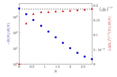
In Fig. 8 and Fig. 9 one can observe the evolution of and its dispersion around the mean value along the non-attractor phase, where the number of e-folds is set to zero at the transition. The procedure followed for the marginalisation over the field is the same as the one previously presented for the case of a linear potential.
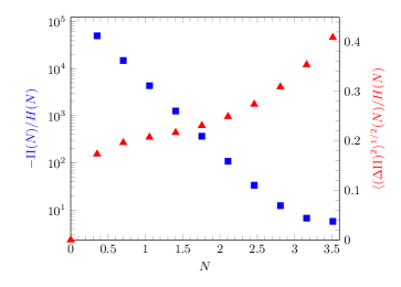
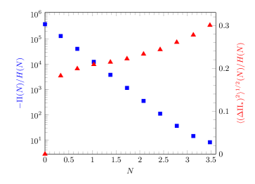
We see that the more the classical value of the inflaton velocity decreases, the more its spread grows with time. The distribution is well-fitted by a Gaussian with spread . In the former model, for example, at the end of the non-attractor phase, we have
| (4.1) |
which is larger than about a factor of two than the variance for the linear potential . We notice instead that the behaviour of the spread is well reproduced by the expression (3.42) even though with deviations near the end of the non-attractor phase.
V. A criterion for the quantum diffusion
As previously discussed, the crucial quantity is the spread of the velocity of the inflaton field for the various trajectories. If the spread of the probability distribution is smaller than the size of the region over which the perturbation is of the order of , then an insignificant part of the wave packet goes out the region where the curvature perturbation is and most of the trajectories will have the same curvature perturbation . We impose therefore the criterion that the spread of the probability distribution is still within the region where , see Fig. 10,
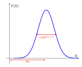
| (5.1) |
Linear potential
For the linear potential during the non-attractor phase, the region where the curvature perturbation has a given value has a width (recall that )
| (5.2) |
and therefore one obtains the criterion
| (5.3) |
If satisfied, we can conclude that along most of the classical trajectories PBH’s can be generated. If not true, this is equivalent to say that the wave-function of the inflaton velocity penetrates into the regions where the velocities are much different from , leading to non-perturbative values of and to a totally random motion if . Of course, one can get a stronger constraint if one imposes that the penetration does not occur at variances, or
| (5.4) |
Now, since
| (5.5) |
we finally obtain
| (5.6) |
More physical cases
For the more realistic models discussed in Refs. [18, 19] our results are provided in Figs. 8 and 9. As we have noticed, the distribution is well-fitted by a Gaussian with spread . As already mentioned, one needs to take the value of the curvature perturbation at the peak at the end of the non-attractor phase since the corresponding mode does not change in time afterwards. Therefore, taking into account that for both cases , we obtain
| (5.7) |
while
| (5.8) |
which is comfortably smaller than (5.7). The criterion is well satisfied thanks to the boost the power spectrum gets at the peak with respect to the power spectrum calculated for the wavelength leaving the Hubble radius deep in the non-attractor phase. However, as we will see next, this does not seem enough for the quantum diffusion not to have an impact on the PBH abundance.
VI. A stronger criterion for the quantum diffusion
The presence of sizeable quantum diffusion enters in another relevant consideration and provides a stronger criterion. Assume a Gaussian form for the PBH mass function
| (6.1) |
Suppose one fine-tunes the parameters of the inflaton potential to produce the right amount of PBH as dark matter, but without accounting for the quantum diffusion and therefore the spread of the inflaton velocities.
Practitioners of the production of PBHs as dark matter in single-field models of inflation know that a considerable fine-tuning is needed in any model to produce the right amount of dark matter in the form of PBHs. Any deviation from the fine-tuned set of parameters due to the uncertainty caused by the quantum diffusion will lead to huge variations of the PBH primordial mass fraction (as well as the ignorance on the non-Gaussian corrections do). Let us take therefore into account the spread now on the PBH mass fraction itself.
Linear potential
Assuming that , the PBH mass fraction has an average induced by quantum diffusion equal to
| (6.2) |
Using a Gaussian distribution for with spread , we get
| (6.3) |
Notice that the average value of the PBH primordial abundance gets shifted with respect to the expression (6.1) precisely because the distribution of the inflaton velocity has a nonvanishing width.
We may define a fine-tuning parameter defined through the ratio of the averaged mass fraction in the presence of diffusion and the mass fraction in the absence of diffusion as
| (6.4) |
Essentially, this fine-tuning parameter says how far is the average of the distribution of from the classical value computed in the absence of quantum diffusion. We find that
| (6.5) |
Imposing that the calculation is done in the absence of diffusion is trustable requires , or
| (6.6) |
For a linear potential this bound is violated by the fact that the spread in the velocity is . One might think to reduce the fine-tuning by, for instance, decrease the value of , however one should also recall that in order to get the right amount of dark matter in the form of PBH, , one needs and therefore decreasing leads to a strong decrease in . Alternatively, one can fix the spread in the velocity to be and, imposing , find a lower bound on the square root of the variance
| (6.7) |
which signals the difficulty of avoiding the impact of the quantum noise.
Non-attractor: more physical cases
For a more realistic potential, like the one in Ref. [18], we have seen that the spread in the velocities at the end of the non-attractor phase is as large as . To assess the impact of the quantum diffusion on the PBH abundance, we have proceeded as follows. We have set the parameters of the model as in section II, see Tab. 1, in such a way to reproduce the right abundance for the PBHs to be dark matter and for the potential to be consistent with the CMB constraints on the power spectrum at the reference scale of (the spectral index and the tensor to scalar ratio computed in the slow-roll region are as well in agreement with current data).
The PBH abundance has been calculated using the density contrast with threshold [26] where the variance is defined as
| (6.8) |
where is a Gaussian window function smoothing out the density contrast on the comoving horizon length . The Gaussian approximation of the primordial mass fraction
| (6.9) |
gives and therefore the right dark matter abundance. We have then included the quantum diffusion, run realisations of the stochastic background evolution and for each of them we have calculated the primordial PBH abundance .
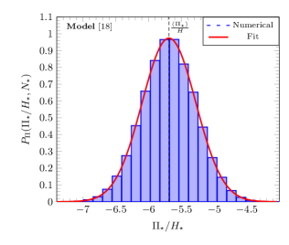
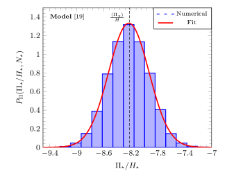
Our results show that is approximately Gaussian distributed around the value of computed using the classical inflaton evolution, and with a standard deviation , see Fig. 11. This is only an approximation because there is a small skewness shifting the average slightly away from its classical value. This means that is nearly distributed as a log-normal distribution. Extending what we have done previously, we can introduce a fine-tuning parameter defined to be
| (6.10) |
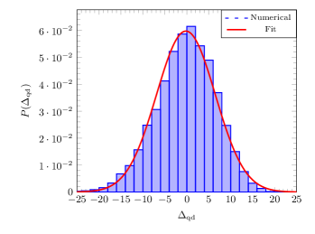

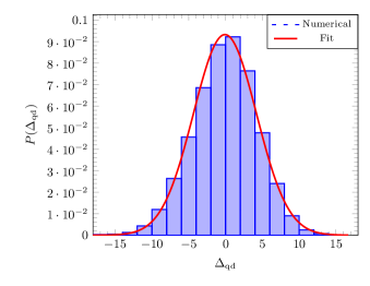
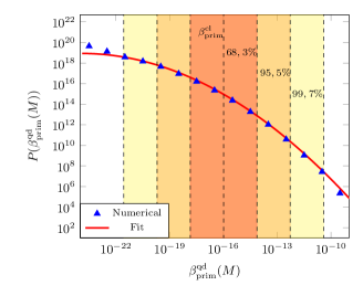
This quantity is distributed like a Gaussian and is a measure of how close the distribution of the PBH mass fraction is peaked around the classical value. Therefore is (nearly) centered around zero and within it acquires values
| (6.11) |
The values of are summarised in Tab. 2. Notice that the range is not totally symmetric because of the small skewness.
| Model [18] | ||||||
|---|---|---|---|---|---|---|
| Model [19] | ||||||
We observe that the criterion is grossly violated and the value of violently deviates from the classical value due to the effect of quantum diffusion on the evolution of the background. In other words the values of the PBH mass fraction violently fluctuate around an average which is very different from the classical value thought to be needed to get the right abundance of the dark matter in the form of PBH.
Similar results are obtained for the model in Ref. [19], they are shown in Fig. 12. For the sake of comparison we have used the same reference values as in Ref. [19]. We notice that the dispersion of is less prominent. However, this is only due to the fact that in Ref. [19] a smaller threshold, , has been adopted, leading to smaller values of the variances to reproduce the right amount of dark matter in the form of PBHs. As a consequence, the impact of quantum diffusion is relatively smaller. Still, the criterion is violated as we can see from Tab. 2. We also remark that higher values of [26] are used in the literature and therefore even larger values of will be obtained.
Our results make us confident that, while in principle conclusions might depend on the exact values of the square root of the variance and threshold , the corresponding will in general be too large. This is because changing the parameters of the model to get new variances with some new thresholds does not reduce significantly the spread of . Therefore, while our results are specific of the models we have considered, we believe the conclusions apply to any model where the inflaton field crosses a plateau with an inflection point in order to generate a spike in the power spectrum and give rise to PBHs.
We expect therefore that the standard (classical) picture to evaluate the dark matter abundance in terms of PBHs is significantly altered.
VII. Conclusions
There is a lot of interest in the cosmology community for the possibility that the dark matter is formed by PBHs. Their origin might be ascribed to the same mechanism giving rise to the CMB anisotropies and large-scale scale structure, i.e. a period of inflationary accelerated expansion during the early stages of evolution of the universe. In single-field models the power spectrum of the curvature perturbation might increase at small scales if the inflaton crosses a region which is flat enough and various models in the literature have been proposed recently.
In this paper we have discussed the role of quantum diffusion in the determination of the final abundance of PBHs. Quantum diffusion necessarily acquires importance when the force induced by the inflaton potential becomes tiny during the dynamics of the inflaton field. We have analysed both analytically and numerically the impact of diffusion and concluded that in realistic models it can significantly affect the capability of making a firm prediction of the PBH abundance. This is because the velocity of the inflaton field turns out to be distributed around its classical value with a spread which has an exponential impact on the PBH mass fraction.
While by itself the mass fraction does not say anything about the spatial distribution of the PBHs, we expect that different regions of the universe upon PBH formation would be populated with different relative abundances, thus changing the prediction for how much dark matter there is or its subsequent evolution.
Acknowledgments
We thank M. Cicoli, F. G. Pedro, and G. Tasinato for many interactions about their work (Refs. [18] and [19] respectively) and feedback on our draft. We also thank A. Linde for interactions about the PBH formation probability. We also thank C. Germani for disscussions. A.R. is supported by the Swiss National Science Foundation (SNSF), project Investigating the Nature of Dark Matter, project number: 200020-159223. A.K. thanks the Cosmology group at the Département de Physique Théorique at the Université de Genève for the kind hospitality and financial support.
Appendix A: the curvature perturbation, the Schwarzian derivative and the dual transformation
In this Appendix we elaborate further the issue of why the power spectrum during the non-attractor phase is indeed flat. This Appendix does not contain some new material with respect to the literature.
Our starting point is the equation for the curvature perturbation on comoving hypersurfaces
| (A.1) |
where for convenience the prime denotes in this Appendix and in the following one the conformal time derivative and (the dot denotes the cosmic time derivative). The function satisfies the following equation
| (A.2) |
where
| (A.3) |
As long as slow-roll is attained, one can make use of the corresponding slow-roll parameters deduced from the form of the potential
| (A.4) |
where the dynamics around Hubble crossing is dominated by the exponentially growing friction term proportional to , and the solution to Eq. (A.1) is well approximated by
| (A.5) |
where indicates the value of the conformal time at which the comoving wavelength leaves the comoving Hubble radius.
In the case in which one is interested in the generation of PBH from sizeable curvature fluctuations at small scales, a violent departure from the slow-roll must occur. In particular, if after Hubble crossing the friction term proportional to changes its sign from positive to negative, it may become a driving term. This can have significant effects on modes which leave or have left the Hubble radius during this transient and non-attractor epoch and thus induce a growth of the curvature perturbations [58, 57]. A necessary, but not sufficient condition, to have PBH generation from single-field models is therefore the presence of a transient period for which
| (A.6) |
During such stage the function reaches a local extremum (a maximum or a minimum depending upon the sign of ) at some time whenever
| (A.7) |
Since is always positive, the presence of a transient stage implies that must be at least unity, signalling a breakdown of the slow-roll conditions.
In order to simplify the problem of dealing with a non-attractor phase necessary to generate a large amount of PBHs, we start by noticing that, upon the redefinition
| (A.8) |
the quantity satisfies the same equation of
| (A.9) |
as long as
| (A.10) |
The transformation from to which satisfies the relation (A.10) has been nicely worked out in Ref. [55] and called a dual transformation. It reads
| (A.11) |
In fact this transformation is a property inferred from the so-called Schwarzian derivative [60], which we briefly summarise in the next subsection
The Schwarzian derivative
Given a function , the Schwarzian derivative is defined as
| (A.12) |
A property of the Schwarzian is that it is invariant under the transformation
| (A.13) |
that is
| (A.14) |
Note that the symmetry (A.14) is just SL up to a rescaling of . Consider now a differential equation
| (A.15) |
It can easily be seen that
| (A.16) |
where
| (A.17) |
Indeed, from Eq. (A.17) we find that
| (A.18) |
and therefore,
| (A.19) |
which is nothing else than Eq.(A.15) and Eq. (A.16). Now, since the Schwarzian is invariant under the transformation (A.13), we have that
| (A.20) |
where
| (A.21) |
Then, using Eqs. (A.13), (A.18) and (A.21) we find that
| (A.22) |
which, by using Eq.(A.17), is written as
| (A.23) |
which is nothing else than the dual transformation found in Ref. [55].
Going back to the transformation (A.11), the power spectrum of the comoving curvature perturbation at the end of inflation reads
| (A.24) |
from which we deduce that the power spectrum of the comoving curvature perturbation is flat, a property that is inherited by the power spectrum of for which the dynamics is of the slow-roll nature. The question now is what is the most suitable dual transformation to perform in order to simplify the computation of the power spectrum for those modes which exit the Hubble radius during the non-attractor phase and which are ultimately responsible for the production of PBHs when these curvature perturbations re-enter the Hubble radius during the radiation phase.
As we have mentioned already several times, the production of PBHs may originated from the enhancement of the curvature power spectrum below a certain length scale. This can be achieved by a temporary abandonment of the slow-roll condition. When the inflaton field follows slow-roll and is approximately constant, the function grows
| (A.25) |
During the non-attractor phase, when the inflaton field experiences an approximately flat potential and can be neglected, it satisfies the equation of motion
| (A.26) |
and consequently , or
| (A.27) |
It is this rapid fall of which allows the possibility of enhancing the power spectrum. When the non-attractor phase is over, the slow-roll conditions are attained again and one recovers the behaviour in Eq. (A.25). In terms of the friction term one has
| (A.28) |
Let us now use the dual transformation (A.11) where we choose the lower limit of the integral to be , the initial conformal time for the non-attractor phase. In such a case, we find
| (A.29) |
We can now choose and compute this expression during the non-attractor phase for those modes which enter the Hubble radius during the non-attractor phase
| (A.30) |
Setting and , we obtain
| (A.31) |
where in the last passage we have neglected the subleading term . Taking (recall that ) and recalling that , one finally obtains
| (A.32) |
This demonstrates that the choice
| (A.33) |
maps the non-attractor phase into a slow-roll phase for the curvature perturbation and one can conclude that the power spectrum of the curvature perturbation for those modes entering the Hubble radius during the non-attractor phase is dictated by a slow-roll dynamics and therefore is flat. Its amplitude is however magnified by a factor .
To elaborate further and find a useful prescription, let us consider, as we also did in the main text, Starobinsky’s model [59] where the inflaton field reaches a non-attractor phase after a slow-roll era (and eventually enters afterwards another slow-roll phase).
Slow-roll phase before the non-attractor phase
If we indicate by the moment at which the first slow-roll phase ends and the non-attractor phase starts, we can Taylor expand the inflaton potential as
| (A.34) |
where is the slow-roll parameter during the first slow-roll phase. The corresponding parameter reads
| (A.35) |
having indicated and is the conformal time and the scale factor when , respectively.
Non-attractor phase
For the potential is Taylor expanded as
| (A.36) |
The dynamics leads to
| (A.37) |
and
| (A.38) |
If , there is a prolonged non-attractor phase where the second term in the above equation dominates over the first one. It is easy to show that reaches a maximum at the point
| (A.39) |
corresponding to and causing a sizeable change in on super-Hubble scales if is very tiny. Notice that the smallness of parametrises the duration of the non-attractor phase from to . Let us now consider the duality transformation (A.11) with again lower limit in the integral. We deduce
| (A.40) |
We are free to choose such that the second term on the right-hand side of Eq. (A.40) vanishes, which happens for
| (A.41) |
and hence
| (A.42) |
We are also free to make the dual transformation only for and therefore we match with the new at and find
| (A.43) |
Therefore we have a single slow-roll parameter
| (A.44) |
throughout all the evolution. This implies that the power spectrum for the not only remains constant after Hubble crossing, but also can be computed using the slow-roll approximations and it reads
| (A.45) |
even during the non-attractor phase. The power spectrum therefore evolves as
| (A.46) |
Defining by the end of the non-attractor phase and computing the power spectrum just after (recall that the conformal time is negative and therefore )) we find that immediately after the non-attractor phase
| (A.47) |
At the end of the non-attractor phase therefore one finds
| (A.48) |
which provides the prescription to compute the power spectrum of the curvature perturbations for those modes crossing the Hubble radius deep in the non-attractor phase. By tuning the slope of the potential one can in principle obtain a large enhancement of the power spectrum.
A few comments are in order. The last passage in Eq. (A.48) is valid only if the subsequent slow-roll phase starts when the velocity of the inflaton field has already settled to its slow-roll value proportional to . We remind the reader that the power spectrum does not further evolve during the subsequent transition between the non-attractor phase and the second slow-roll phase [39]. The prescription (A.48) was already proposed in Ref. [56] (see also Refs. [55, 57, 58]) to deal with the singular case in which . In this sense the results of this long Appendix are not new, but we have given an alternative and maybe more intuitive derivation. Furthermore, the prescription (A.48) can be used for those modes which exit the Hubble radius deep in the non-attractor phase and predicts a flat power spectrum as the dual experiences a slow-roll dynamics. Said in other words, the power spectrum must be flat since up to small correction . If one wishes to compute the abundance of PBHs using single-field models where a non-attractor phase is necessary, the corresponding power spectrum of the comoving curvature perturbation can be computed by simply evaluating it at Hubble crossing, even during the non-attractor phase, as long as one makes use of the slow-roll relation ; one can then account for the modes leaving the Hubble radius when grows fast from tiny values to 3 using Eq. (Non-attractor: some analytical considerations). Finally, the prescription is based on the fact that the non-attractor phase is long enough for the dynamics to established. If the plateau is short in field space, the inflaton field may arrive at it with an excessive kinetic energy and roll away of it in a Hubble time or so.
Appendix B: from the non-attractor back to the slow-roll phase
The modes which have crossed the Hubble radius during the non-attractor phase are on super-Hubble scales during the eventual subsequent transition to a slow-roll phase with larger slope in the potential. To see what happens to these modes we follow Ref. [39] and model again the potential during the transition as
| (B.1) |
where we have defined the field value at the end of the attractor phase. The equation of motion for the inflaton field during the transition epoch reads
| (B.2) |
whose solution for initial velocity leads to
| (B.3) |
The solution for the super-Hubble scale comoving perturbation during the transient epoch reads
| (B.4) |
This solution needs to be matched now with the solution for which (apart from the standard scales like . Matching the perturbations and their derivatives at , one gets
| (B.5) |
We see that if the non-attractor phase is followed by another slow-roll phase for which , the curvature perturbations associated to the modes which are on super-Hubble scales during the transition will keep be enhanced as and the prescription (A.48) remains valid for those modes exiting the Hubble radius deep in the non-attractor phase [39].
Appendix C: the role of non-Gaussianities
As we mentioned in the introduction, PBHs are born as large, but rare fluctuations of the curvature perturbation. As such, their abundance is extremely sensitive to the non-linearities of the curvature perturbation. A formalism particularly useful when dealing with non-linearities is the so-called formalism [51], where the scalar field fluctuations are quantized on the flat slices and , being the number of e-folds. The formalism is based on the assumption that on super-Hubble scales, each spatial point of the universe has an independent evolution and the latter is well approximated by the evolution of an unperturbed universe.
Let us suppose that during the entire non-attractor phase the inflaton velocity decays exponentially. If so
| (C.1) |
where is again the value of the field at the end of the non-attractor phase. Notice that we have retained the dependence on since slow-roll is badly violated. In the relation (D.3) we have followed the notation of Ref. [39] and defined to be the end of the attractor phase, so that and
| (C.2) |
We therefore find that
| (C.3) |
where the overlines indicate the corresponding background values. One can safely neglect the perturbation as it decays exponentially fast. On the other hand, by using the relation
| (C.4) |
we see that up to irrelevant constants,
| (C.5) |
The crucial point now is that the dynamics of is the one of a massless perturbation in de Sitter and to a very good approximation its behaviour is Gaussian. The non-Gaussianity in the curvature perturbation arises because of the non-linear mapping between and 111A few comments. The non-Gaussianity during the non-attractor phase is not washed out by the subsequent transition to a slow-roll phase. This is because such a transition is sudden [39] as the velocity during the non-attractor phase must be much smaller than the one during the subsequent slow-roll phase to generate PBHs. The non-Gaussianity we are dealing with here is not the non-Gaussianity in the squeezed configuration which peaks when one of the wavelengths is much larger than the other two. This non-Gaussianity is not observable by a local observer testing a region much smaller than the long wavelength [63]. We are instead referring to that non-Gaussianity which arises at the same small wavelengths where the density perturbations are sizeable. In the limit of a spiked power spectrum centered around a given momentum , the non-Gaussianity will be peaked at equilateral configurations..
The fact that is Gaussian considerably simplifies the computation: the primordial mass fraction of the universe occupied by PBHs at formation time is dictated by probability conservation,
| (C.6) |
or
| (C.7) |
where we have written the Gaussian distribution of as222Sometimes the Gaussian probability is multiplied by a factor of 2 to account for the fact that one deals with a first time-passage problem [62]. We do not put it here as there is no general consensus of this factor. Quantitatively, it does not make a big difference though.
| (C.8) |
with
| (C.9) |
For , we obtain
| (C.10) |
i.e., a Gaussian with variance
| (C.11) |
On the other hand, assuming now , we obtain
| (C.12) | |||||
to be confronted to the Gaussian result (6.9). The probability is clearly non- Gaussian. We can estimate as well to be of the order of . We obtain
| (C.13) |
To obtain the same primordial mass fraction, non-Gaussianity seems to require a smaller . We write “seems” as the curvature perturbation is not the best variable to study the PBH mass function. As written in the main text, the density contrast (during radiation) is the good variable [26]. This however will make things more difficult to analyse because of the complication arising from taking the laplacian of the expression (C.3). One possible, but not entirely satisfactory, way out might to evaluate the density contrast at Hubble re-entry, i.e. setting . In such a case, one could relate the density contrast to the curvature perturbation through the relation .
Appendix D: Comment on 1807.09057
After the publication of this paper, Ref.[64] appeared with some comments about our findings. Here we respond to them. This Appendix can be considered as an independent part of this work and therefore some concepts of the main text might be repeated.
First of all, to the best of our understanding, Ref. [64] just contains the demonstration that one can compute the curvature perturbation in the non-attractor phase using the stochastic approach instead of adopting the standard computation in curved spacetime quantum field theory. This result differs from that in Ref. [65] and this is reassuring, as the standard linear computation has been our starting point333However, we stress that one can exactly map by duality the non-attractor phase into a slow-roll phase in the limit of a plateau in the potential (see Ref. [55] and Appendix A). This makes the conclusions of Ref. [64] suspicious, as they claim that the non-attractor phase and the slow-roll phase behave differently at leading order in the slow-roll parameters.. In our paper, however, we have not used the stochastic approach to compute the perturbations, but to investigate the role of quantum diffusion on the observables. We did not assume the validity of the stochastic approach to compute the perturbations, the latter being derived by the standard field theory techniques (as in the large majority of the literature on the non-attractor phase).
The stochastic approach to study the cosmological perturbations focus on the behaviour of the perturbations on large scales under the action of the short modes which are integrated out from the action. These long mode perturbations are then treated classically under the action of a stochastic noise and give rise to a given power spectrum. In our approach, we do not focus on the perturbations, but on the effect of the noise onto the background observables.
Our results have therefore little to do with those in Ref. [64]. In fact, the importance of diffusion in the determination of the primordial PBH abundance has been already discussed in Ref. [49] where it was also shown to be crucial (their analysis is restricted to slow-roll. However in the limit of extreme flatness of the potential during the non-attractor phase one can apply the duality discussed in Ref. [55] and in our Appendix A to map the problem into a slow-roll one).
Nevertheless, let us provide some comments about the criticisms raised in Ref. [64]. This will also allow us to discuss some clarifications/considerations.
The point raised in Ref. [64] is that the power spectrum is not a stochastic quantity and therefore may not be used to calculate the impact of quantum diffusion onto the PBH abundance. However, the smoothed power spectrum (the one which enters in the calculation of the abundance of PBHs) is a stochastic quantity once one specifies the scale at which the average is operated and in the presence of long-mode perturbations with wavelengths larger than the size of the region where the averaged is performed. This is nicely explained, for instance, in Ref. [66]. Let us consider two counter-examples to the statement of Ref. [64]. First, the computation of the celebrated Maldacena consistency relation relating the power spectra of the curvature perturbation to the bispectrum in the squeezed limit. It is well-known that such a result may be obtained simply taking the power spectrum, computed on a small box, and average it over a bigger volume containing the long-mode perturbation. The very simple result that the power spectrum correlates with the long mode shows that it is not a function, but a stochastic quantity. Similarly, in order to compute the local halo bias in the presence of primordial non-Gaussianity one exploits the fact that the variance of the density contrast is stochastic quantity in the presence of long-mode perturbations.
As we explain in the main text, one way of producing PBHs in the early universe is to generate an enhancement of the power spectrum of the curvature perturbation during inflation, more specifically during the non-attractor. These large perturbations re-enter the horizon during the radiation era and may collapse to form PBHs on comoving scales that left the Hubble radius about e-folds before the end of inflation.
At the end of the non-attractor phase the curvature perturbation (in the flat gauge) is
| (D.1) |
The calculation of the curvature perturbation till the end of the non-attractor can be performed by using the formalism [39]. Let us suppose that during the entire non-attractor phase the inflaton velocity decays exponentially so that
| (D.2) |
Here and are the values of the inflaton field and its velocity at the end of the non-attractor phase, respectively and we have set to be the end of the attractor phase, so that . Then
| (D.3) |
On the other hand, by using the relation (D.2) and expanding at first-order one finds the expression (D.1). Now, in this paper we have followed the same logic which has been neatly explained in Ref. [13]. The method consists of three steps [13]:
-
•
First of all, to find an inflationary trajectory for any point in the space and to calculate the number of e-folds for this trajectory.
-
•
The position of the point has to be perturbed by adding to it inflationary jumps. This provides the perturbation of the number of e-folds , which is directly related to the density perturbations.
-
•
The third step and most relevant for us (usually not performed in slow-roll single-field models) comes from the fact that the resulting density perturbation for a given (i.e. for a given wavelength) will depend on the place the trajectory come from. Thus the remaining step is to evaluate the probability that for a given number of e-folds till the end of the non-attractor phase (usually till the end of inflation in slow-roll models) the field was at any particular point . This is because for an observer restricted to her/his own Hubble radius during inflation, the classical value of the field is not given only by the zero mode, but also by the sum of the modes with wavelength larger than the Hubble length. This was the essence of the results of Ref. [49] which indeed found that the PBH abundance is different when quantum diffusion is present. The necessity of such third sanity-check step was also stressed in Ref. [66] (even though with no reference to PBHs).
As pointed out also in Ref. [13], this third step can be performed by using the stochastic approach which tells what is the probability to find a given value of the inflaton field and its velocity at a given point as a function of time.
In the main text we have pointed out that during the non-attractor phase the role of quantum diffusion on the coarse-grained field may become relevant and changes the value measured by observers restricted to their own Hubble patches. In other words, we have pointed out that the last and third sanity-check step described above is necessary. Usually in slow-roll single-field models probabilities are basically Gaussian functions peaked around the classical values and tiny widths and one neglects the third step (even though for the problem of the PBH abundance is indeed necessary [49]).
In order to compute the variance of the sizeable curvature perturbation upon horizon re-entry, which will eventually give rise to PBHs by collapse, one usually considers the classical evolution of the homogeneous fields and and the effect of perturbations about the classical trajectories on a given scale. However, in the extreme case in which diffusion overcomes the classicality, one may not estimate the curvature perturbation in terms of the classical trajectories [13]. Luckily, in the case at hand, quantum diffusion never becomes more relevant than its classical evolution. Nevertheless, even tiny differences may have an impact on the final abundance of the PBHs as it is exponentially sensitive to the variance deduced from power spectrum of .
In order to calculate the probability distribution for the field we have used the stochastic approach which amounts to assuming an average quantum diffusion per Hubble volume per Hubble time of the order of . The velocity of the inflaton field becomes also a stochastic variable and the corresponding variance characterises the dispersion of the classical trajectories due to quantum fluctuations.
Taking for simplicity the case of constant potential during the non-attractor phase, the stochastic equations are (we report them here)
| (D.4) |
where and we have indicated with and . This set of equations shows that, even if the inflaton field and its velocity are taken to be homogeneous till one e-fold before the end of the non-attractor phase, it is unavoidable that at the end of it the inflaton field receives kicks of the order of
| (D.5) |
and the velocity of the order of
| (D.6) |
In slow-roll one does not worry about these kicks, as the classical value of the velocity is given by , where is a slow-roll parameter and the reduced Planck mass. This effect is totally negligible. However, at the end of the non-attractor phase is much smaller, . The variance of the inflaton velocity is not negligible when recalling that tiny changes of the curvature perturbations are exponentially inflated when computing the PBH abundance.
Notice that the variance of the inflaton velocity reaches the value (D.6) after one e-fold or so, and remains the same on all coarse-grained lengths. In particular, assuming that the peak of the perturbation is reached, say, 20 e-folds before the end of inflation, our current universe will contain, at the time of formation of the PBHs, about Hubble volumes. In any of them the velocity has tiny differences due to the variance (D.6). Since the probability to form a PBH in any of each patches is Eq. (1.1), having a not fully fixed leads to different values of and therefore in all the patches. One point to stress is that the kicks (D.6) are kicks of the short modes leaving the Hubble radius each Hubble time and what they do is to change the infrared long modes of the inflaton velocity whose cumulative effect is measured by the local observer as the background inflaton velocity.
Thus, while the final word is certainly given by the calculation of the exact probability of the comoving curvature perturbation and the corresponding KM-like equation (see for example Ref. [67] for the slow-roll case), in order to avoid any analytical approximation, we have numerically constructed different realisations of the comoving curvature perturbation by solving the corresponding equation of motion (A.1) for any given wavenumber, one for each random trajectory identified by the corresponding coarse-grained background values. We have then deduced the mean and the variance of the abundance of the PBHs. These procedures are equivalent.
As a final note, let us stress that the fact that the density contrast barrier depends on the shape of the power spectrum (which in turn determines the shape of the perturbation in real space collapsing to a PBH) implies that a change in the comoving curvature perturbation in each Hubble patch at horizon re-entry due to quantum diffusion will determine a different barrier. This as well is expected to have an impact on the final PBH abundance distribution.
References
- [1] B. J. Carr and S. W. Hawking, Mon. Not. Roy. Astron. Soc. 168, 399 (1974).
- [2] P. Meszaros, Astron. Astrophys. 37, 225 (1974).
- [3] B. J. Carr, Astrophys. J. 201, 1 (1975).
- [4] S. Bird, I. Cholis, J. B. Muñoz, Y. Ali-Haïmoud, M. Kamionkowski, E. D. Kovetz, A. Raccanelli and A. G. Riess, Phys. Rev. Lett. 116, no. 20, 201301 (2016) [astro-ph.CO/1603.00464].
- [5] S. Clesse and J. GarcÃa-Bellido, Phys. Dark Univ. 15, 142 (2017) [astro-ph.CO/1603.05234].
- [6] M. Sasaki, T. Suyama, T. Tanaka and S. Yokoyama, Phys. Rev. Lett. 117, no. 6, 061101 (2016) [astro-ph.CO/1603.08338].
- [7] M. Sasaki, T. Suyama, T. Tanaka and S. Yokoyama, [astro-ph.CO/1801.05235].
- [8] B. Carr, M. Raidal, T. Tenkanen, V. Vaskonen and H. VeermÂe, Phys. Rev. D 96, no. 2, 023514 (2017) [astro-ph.CO/1705.05567].
- [9] M. Zumalacarregui and U. Seljak, [astro-ph.CO/1712.02240].
- [10] J. Garcia-Bellido, S. Clesse and P. Fleury, [astro-ph.CO/1712.06574]
- [11] B. P. Abbott et al. [LIGO Scientific and Virgo Collaborations], Phys. Rev. Lett. 116, 061102 (2016) [gr-qc/1602.03837].
- [12] P. Ivanov, P. Naselsky and I. Novikov, Phys. Rev. D 50, 7173 (1994).
- [13] J. García-Bellido, A.D. Linde and D. Wands, Phys. Rev. D 54 (1996) 6040 [astro-ph/9605094].
- [14] P. Ivanov, Phys. Rev. D 57, 7145 (1998) [astro-ph/9708224].
- [15] J. Garcia-Bellido and E. Ruiz Morales, Phys. Dark Univ. 18, 47 (2017) [astro-ph.CO/1702.03901].
- [16] K. Kannike, L. Marzola, M. Raidal and H. VeermÂe, JCAP 1709, no. 09, 020 (2017) [astro-ph.CO/1705.06225].
- [17] G. Ballesteros and M. Taoso, Phys. Rev. D 97, no. 2, 023501 (2018) [hep-ph/1709.05565].
- [18] M. Cicoli, V. A. Diaz and F. G. Pedro, [hep-th/1803.02837].
- [19] O. Özsoy, S. Parameswaran, G. Tasinato and I. Zavala, [hep-th/1803.07626].
- [20] M. Kawasaki, N. Kitajima and T. T. Yanagida, Phys. Rev. D 87, no. 6, 063519 (2013) [hep-ph/1207.2550].
- [21] B. Carr, F. Kuhnel and M. Sandstad, Phys. Rev. D 94, 083504 (2016) [astro-ph.CO/1607.06077].
- [22] J. Garcia-Bellido, M. Peloso and C. Unal, JCAP 1612, no. 12, 031 (2016) [astro-ph.CO/1610.03763].
- [23] B. Carr, T. Tenkanen and V. Vaskonen, Phys. Rev. D 96, no. 6, 063507 (2017) [astro-ph.CO/1706.03746].
- [24] J. R. Espinosa, D. Racco and A. Riotto, Phys. Rev. Lett. 120, 121301 (2018) [hep-ph/1710.11196].
- [25] T. Harada, C. M. Yoo and K. Kohri, Phys. Rev. D 88, 084051 (2013), Erratum: [Phys. Rev. D 89, 029903 (2014)], [astro-ph.CO/1309.4201].
- [26] S. Young, C. T. Byrnes, and M. Sasaki, JCAP 1407, 045 (2014) [gr-qc/1405.7023].
- [27] I. Musco and J. C. Miller, Class. Quant. Grav. 30, 145009 (2013) [gr-qc/1201.2379].
- [28] H. Motohashi and W. Hu, Phys. Rev. D 96, no. 6, 063503 (2017) [astro-ph.CO/1706.06784].
- [29] D.H. Lyth and A. Riotto, Phys. Rept. 314 (1999) 1 [hep-ph/9807278].
- [30] W. H. Kinney, Phys. Rev. D 72, 023515 (2005) [gr-qc/0503017].
- [31] C. Dvorkin and W. Hu, Phys. Rev. D 81, 023518 (2010) [astro-ph.CO/0910.2237].
- [32] M. H. Namjoo, H. Firouzjahi, and M. Sasaki, Europhys. Lett. 101, 39001 (2013) [astro-ph.CO/1210.3692].
- [33] J. Martin, H. Motohashi and T. Suyama, Phys. Rev. D 87, no. 2, 023514 (2013) [astro-ph.CO/arXiv:1211.0083].
- [34] X. Chen, H. Firouzjahi, M. H. Namjoo and M. Sasaki, EPL 102, no. 5, 59001 (2013) [hep-th/1301.5699].
- [35] S. Mooij and G. A. Palma, JCAP 1511, no. 11, 025 (2015) [astro-ph.CO/arXiv:1502.03458].
- [36] C. Germani and T. Prokopec, Phys. Dark Univ. 18, 6 (2017) [astro-ph.CO/1706.04226].
- [37] K. Dimopoulos, Phys. Lett. B 775, 262 (2017) [hep-ph/1707.05644].
- [38] B. Finelli, G. Goon, E. Pajer and L. Santoni, Phys. Rev. D 97, no. 6, 063531 (2018) [hep-th/1711.03737].
- [39] Y. F. Cai, X. Chen, M. H. Namjoo, M. Sasaki, D. G. Wang and Z. Wang, [astro-ph.CO/1712.09998].
- [40] J.M. Ezquiaga, J. García-Bellido and E. Ruiz Morales, Phys. Lett. B 776, 345 (2018) [astro-ph.CO/1705.04861].
- [41] S. Young and C. T. Byrnes, JCAP 1308, 052 (2013) [astro-ph.CO/1307.4995].
- [42] E. V. Bugaev and P. A. Klimai, Int. J. Mod. Phys. D 22, 1350034 (2013) [astro-ph.CO/1303.3146].
- [43] J. S. Bullock and J. R. Primack, Phys. Rev. D55, 7423 (1997) [astro-ph/9611106].
- [44] J. Yokoyama, Phys. Rev. D58, 083510 (1998) [astro-ph/9802357].
- [45] R. Saito, J. Yokoyama, and R. Nagata, JCAP 0806, 024 (2008) [astro-ph.CO/0804.3470].
- [46] C. T. Byrnes, E. J. Copeland and A. M. Green, Phys. Rev. D 86, 043512 (2012) [astro-ph.CO/1206.4188].
- [47] S. Young, D. Regan, and C. T. Byrnes, JCAP 81602, 029 (2016) [astro-ph.CO/1512.07224].
- [48] M. Kawasaki and Y. Tada, JCAP 1608, 041 (2016) [astro-ph.CO/1512.03515].
- [49] C. Pattison, V. Vennin, H. Assadullahi, and D. Wands, JCAP 1710 046 (2017) [hep-th/1707.00537].
- [50] G. Franciolini, A. Kehagias, S. Matarrese and A. Riotto, JCAP 1803, no. 03, 016 (2018) [astro-ph.CO/1801.09415].
- [51] M. Sasaki and E. D. Stewart, Prog. Theor. Phys. 95, 71 (1996) [astro-ph/9507001].
- [52] A. D. Linde, Contemp. Concepts Phys. 5, 1 (1990) [hep-th/0503203].
- [53] H. Risken, 1984, “The Fokker-Planck equation”, Springer-Verlag, Berlin.
- [54] R.F. Pawula, Phys. Rev. D162, 186 (1967).
- [55] D. Wands, Phys. Rev. D 60, 023507 (1999) [gr-qc/9809062].
- [56] O. Seto, J. Yokoyama and H. Kodama, Phys. Rev. D 61, 103504 (2000) [astro-ph/9911119].
- [57] S. M. Leach, M. Sasaki, D. Wands and A. R. Liddle, Phys. Rev. D 64, 023512 (2001) [astro-ph/0101406].
- [58] S. M. Leach and A. R. Liddle, Phys. Rev. D 63, 043508 (2001) [astro-ph/0010082].
- [59] A. A. Starobinsky, JETP Lett. 55, 489 (1992).
- [60] Nehari, Zeev, Conformal mapping, Dover Ed, pp. 189Ã226, (1952) ISBN.
- [61] M. Sasaki and E. D. Stewart, Prog. Theor. Phys. 95, 71 (1996) [astro-ph/9507001].
- [62] M. Maggiore and A. Riotto, Astrophys. J. 711, 907 (2010) [astro-ph.CO/0903.1249].
- [63] R. Bravo, S. Mooij, G. A. Palma and B. Pradenas, [astro-ph.CO/1711.05290].
- [64] D. Cruces, C. Germani, and T. Prokopec, [astro-ph.CO/1807.09057 ].
- [65] J. M. Ezquiaga and J. García-Bellido, [astro-ph.CO/1805.06731].
- [66] D. H. Lyth, JCAP 0712, 016 (2007) [astro-ph/0707.0361].
- [67] A. Riotto and M. S. Sloth, JCAP 1110, 003 (2011) [astro-ph.CO/1103.5876].