On the kinematics of a runaway Be star population

Abstract

We explore the hypothesis that B type emission-line stars (Be stars) have their origin in mass-transfer binaries by measuring the fraction of runaway Be stars. We assemble the largest-to-date catalogue of 632 Be stars with 6D kinematics, exploiting the precise astrometry of the Tycho-Gaia Astrometric Solution (TGAS) from the first Gaia Data Release. Using binary stellar evolution simulations, we make predictions for the runaway and equatorial rotation velocities of a runaway Be star population. Accounting for observational biases, we calculate that if all classical Be stars originated through mass transfer in binaries, then $17.5\%$ of the Be stars in our catalogue should be runaways. The remaining 82.5% should be in binaries with subdwarfs, white dwarfs or neutron stars, because those systems either remained bound post-supernova or avoided the supernova entirely. Using a Bayesian methodology, we compare the hypothesis that each Be star in our catalogue is a runaway to the null hypothesis that it is a member of the Milky Way disc. We find that $13.1^{+2.6}_{-2.4}\%$ of the Be stars in our catalogue are runaways, and identify a subset of 40 high-probability runaways. We argue that deficiencies in our understanding of binary stellar evolution, as well as the degeneracy between velocity dispersion and number of runaway stars, can explain the slightly lower runaway fraction. We thus conclude that all Be stars could be explained by an origin in mass-transfer binaries. This conclusion is testable with the second Gaia data release (DR2).

1 Introduction

Around 17% of B type stars in the Milky Way show emission lines in their spectra (Zorec & Briot, 1997) and are referred to as the classical Be stars. This designation is historically restricted to stars of luminosity class V-III, as proposed by Jaschek et al. (1981). They are believed to originate when a rapidly rotating B star forms a decretion disc (Rivinius et al., 2013), albeit for unknown reasons. The rapid rotation of the central star minimises the velocity that material in the atmosphere must reach in order to form a Keplerian decretion disc. Both pulsations and magnetic fields have been suggested as ways to launch material into a disc (see e.g., Rivinius et al., 2013, and references therein). An alternative is that the Be phenomenon is related to binary interactions. Harmanec (1987) suggested that the disc is formed of material lost by a Roche-lobe filling companion. However, there is little evidence for such a mass-losing companion for most Be stars. Pols et al. (1991) proposed an alternative mechanism, now known as the post-mass-transfer model, whereby mass is transferred to a star by a Roche-lobe filling companion and the angular momentum carried by this material spins the star up to close to critical velocity. This model requires that a star spinning at or near critical velocity can spontaneously form a decretion disc through an unknown mechanism, which could be the pulsations or magnetic fields proposed for single Be star channels.

Evidence for the mass transfer hypothesis comes from the large number of Be star in binaries. These should be Be+NS (neutron star) binaries if the primary explodes as a supernova. If the primary is sufficiently stripped, it may avoid a supernova explosion and be present as a white dwarf or subdwarf star. There are five known Be+sdO binaries (Gies et al., 1998; Peters et al., 2008; Peters et al., 2013; Peters et al., 2016; Wang et al., 2017) and 28 confirmed Be+NS X-ray binaries (Reig, 2011).

Recently, Boubert et al. (2017) conducted a search of ten nearby Galactic supernova remnants for the runaway former companion of the progenitor star. Four candidates in four remnants were identified, one of which, BD+50 3188 in remnant HB 21, was found to be a Be star. Boubert et al. (2017) argued that this was circumstantial evidence both for the runaway candidacy of the star and for the post-mass-transfer model in general.

There are several other recent works which lend support to the post-mass-transfer model. Chernyakova et al. (2017) studied the Be-X-ray binary LSI +61^∘ 303, which has an eccentricity $e>0.5$. They argue that the superorbital variability seen in this system is due to the compact remnant passing through different regions of the Be star disc and so probing material of varying densities. One origin for this large eccentricity could be that the compact remnant was formed in a supernova and received a large natal kick. Another way to produce an eccentric binary is through capture in a dense stellar system, but LSI +61^∘ 303 does not appear to be situated in such an environment. González-Galán et al. (2018) studied SXP 1062, a Be-X-ray binary located in the Small Magellanic Cloud, which is likely associated with the supernova remnant MCSNR J0127-7332. SXP 1062 is the first Be-X-ray binary that is likely residing in its parental supernova remnant. Nazé et al. (2017) examined $\pi$ Aquarii, a 14 solar mass Be star orbited by a 3 solar mass main-sequence companion at 1 AU separation. This system could arise if it was originally a triple and the inner binary merged to form what is now the Be star. The merging could have occurred during common envelope evolution, the compact remnant of the binary might have been kicked into the companion or the inner binary could have remained bound post-supernova and merged at a later point.

Runaway stars are thought to form through one of two channels. In the Binary Supernova Scenario (BSS, Blaauw, 1961), a star is ejected from a binary system by the supernova of its more massive companion. In the Dynamical Ejection Scenario (DES, Poveda et al., 1967), 3- or 4-body encounters during the collapse of a young star cluster cause the ejection of one or more of the stars. It is not known definitively which of these two mechanisms dominates, but the BSS is thought to be more likely to due to the ubiquity of binary systems among massive stars (e.g.Branch & Wheeler, 2017). If Be stars predominantly originate through the post-mass-transfer route, then a significant fraction should also be runaway stars. Rinehart (2000) constructed a sample of 5756 B and 129 Be stars in the Hipparcos dataset (ESA, 1997) and used them to look for differences between the peculiar velocity distribution of B and Be stars, concluding that the distributions are identical to within $1\sigma$ and thus that the post-mass-transfer model is not supported by the data. Berger & Gies (2001) searched for high-velocity Be stars by cross-matching an existing catalogue of Be stars with the Hipparcos catalogue (ESA, 1997). They only considered stars with published radial velocities brighter than $V\approx 9$ to ensure inclusion in Hipparcos. Berger & Gies (2001) classified all stars with a peculiar space velocity greater than $40\;\mathrm{km}\;\mathrm{s}^{-1}$ as high-velocity and hypothesised that they originate either with a supernova that disrupted the progenitor binary or with binary-binary dynamical interactions in young clusters. 23 of the 344 Be stars in their sample have peculiar space velocities greater than $40\;\mathrm{km}\;\mathrm{s}^{-1}$. Because there is substantial mass transfer before the supernova, we expect that most systems remain bound after the supernova and so these numbers could be consistent with the post-mass-transfer model.

The impetus for looking at these problems anew comes from the Gaia satellite, which was launched on 19th December 2013 (Gaia Collaboration et al., 2016a). This is a successor satellite to Hipparcos and is monitoring all objects brighter than $V\approx 20$ over a period of 5 years. It is providing magnitudes, parallaxes, proper motions and broad band colours for over a billion stars. It is a valuable new resource for problems at the intersection between stellar evolution and stellar dynamics. In this paper, we use the Tycho-Gaia Astrometric Solution (TGAS), which is one of the catalogues comprising the Gaia Data Release 1 (Gaia Collaboration et al., 2016b). It uses data from Tycho-2 (Høg et al., 2000) to provide a 30 year baseline for astrometric calculations and provides parallaxes and proper motions on over 2 million stars mostly within $\approx 1$ kpc of the Sun.

Here, we assemble the largest catalogue of Be stars with full six-dimensional kinematics in Sec. 2, exploiting the remarkable precision of the TGAS astrometric catalogue. We predict the runaway velocity distribution for Be stars based on simulations of binary star evolution in Sec. 3, accounting for the observational bias of the catalogue. In Sec. 4, we formulate a Bayesian approach to our problem of estimation of the fraction of Be stars that are runaways from binary supernova. We present our main result that around $13\%$ of the Be stars in our catalogue are consistent with being runaway stars in Sec. 5, and list the 40 most probable examples. Finally, in Sec. 6, we discuss whether our results are consistent with all Be stars originating through the post-mass-transfer channel, and show that we can explain the puzzling lack of Be stars in the high-latitude sample of runaway B stars of Martin (2006). Finally, in the Conclusion, we argue that we can resolve the true number of Be star runaways by applying the Bayesian methodology introduced in Sec. 4 to the second data release of the Gaia satellite.

2 Data

Extracting constraints on the origin of Be stars requires well-measured radial velocities, proper motions and distances. We consider three datasets which satisfy this requirement. The first is from Berger & Gies (2001), the second is a cross-match between the Be Star Spectra database (BeSS) with SIMBAD and the Tycho-Gaia Astrometric Solution (TGAS), and the third is a cross-match of the Be catalogue of Hou et al. (2016) from the Large Sky Area Multi-Object Fibre Spectroscopic Telescope (LAMOST) with TGAS. We then combine and clean these datasets by removing any duplicates, as well as stars with anomalously high radial velocities. Whilst the fraction of runaways among the Be stars is unknown, the fraction of runaway B stars has long been established to be $\approx 2.5$% for stars of type B0–0.5 and declining to $\approx 1.5$% for stars of type B1–B5 (Blaauw, 1961). It is important to note that there is a difference in terminology between theory and observations when it comes to runaway stars. Runaways fractions are calculated observationally by classifying any star with a peculiar velocity greater than $40\;\mathrm{km}\;\mathrm{s}^{-1}$ to be a runaway star, while theoretically any star ejected from a binary by the supernova explosion of the companion can be called a runaway star with the majority having ejection velocities below this value.

2.1 The Berger & Gies sample

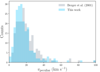
The Berger & Gies (2001) sample contains 344 stars. We first obtain positions and updated radial velocities by querying SIMBAD using the identifiers listed by Berger & Gies (2001). Note that the identifier of the thirteenth star in this sample, CSI+6101449, does not have a cross-match in SIMBAD, but querying Vizier returned the valid identifier HD 10664. For 262 stars, the error on the radial velocity recorded in SIMBAD is smaller than in Berger & Gies (2001). For 320 stars, the radial velocities are consistent within the reported error in the two catalogues. For the other 24 stars, we checked the source of the radial velocity in SIMBAD. Only for HD 120991, where the radial velocity reference was Wilson (1953), did we judge the SIMBAD radial velocity to be less reliable than the Berger & Gies (2001) value. In all other cases, we took whichever radial velocity measurement had the smallest error. The majority of the new radial velocities come from Gontcharov (2006) and Kharchenko et al. (2007). Using the positions, we cross-match with TGAS and obtain more accurate parallaxes and proper motions for 163 of the stars. In Fig. 1, we illustrate the effect of the updated measurements on the peculiar velocity distribution. Note that the peculiar velocities for Berger & Gies (2001) are taken from that work and use a solar radius $R_{\odot}=8.5\;\mathrm{kpc}$, a local circular speed $v_{\mathrm{disc}}=220\;\mathrm{km}\;\mathrm{s}^{-1}$ and a solar peculiar velocity $(U,V,W)_{\odot}=(10.0,5.25,7.17)\;\mathrm{km}\;\mathrm{s}^{-1}$. For the peculiar velocities in this work, we use the more recent values stated in Section 4.

Figure 1: Median peculiar velocities relative to the Milky Way disc of an identical sample of stars using the kinematics from either Berger & Gies (2001) or the catalogue assembled in this work. Thanks to TGAS, the kinematics in our catalogue are more accurate and this produces a significant tightening in the distribution.

2.2 Be Star Spectra database

The Be Star Spectra database (BeSS) claims to be a complete catalogue of classical Be stars and Herbig Ae/Be stars. It contains information on 2265 Be stars and reports radial velocities for 856 and radial velocity errors for 759. After collating this information, we queried SIMBAD to obtain radial velocities, parallaxes and proper motions. SIMBAD provides the proper motion errors in terms of an error ellipse with a major axis $A$, minor axis $B$ and position angle $P$. We convert these to uncertainties in the individual components following the recommended method and neglect the implied covariances. We then carry out a $1\;\mathrm{arcsec}$ nearest neighbour cross-match with TGAS to obtain parallaxes and proper motions. To select whether to use the radial velocity from BeSS or SIMBAD, we pick whichever had the smallest associated error. If the two radial velocities differ by more than $1\sigma$ with respect to their errors added in quadrature, we look at the origin of both measurements and in all cases prefer the radial velocity quoted through SIMBAD. In almost all cases, it was possible to trace the velocity quoted in BeSS back to the General Catalogue of Stellar Radial Velocities and its revision (Wilson, 1953; Evans, 1967). These velocities have been superseded.

2.3 The LAMOST Sample

LAMOST is carrying out a 5 year spectroscopic survey of 10 million Milky Way stars in the Northern hemisphere down to $20.5\;\mathrm{mag}$. Hou et al. (2016) presented a catalogue of 10,436 early-type emission-line stars which are in LAMOST. This catalogue is available as a value-added catalogue of LAMOST DR2. We carry out a $1\;\mathrm{arcsec}$ nearest neighbour cross-match with the LAMOST DR2 stellar catalogue to obtain the reported radial velocities with errors and with TGAS to obtain the parallax $\omega$ and proper-motions $(\mu_{\alpha\ast},\mu_{\delta})$. This results in a total of 12 stars. We add $6.76\;\mathrm{km}\;\mathrm{s}^{-1}$ to correct for the offset found between LAMOST and SDSS SEGUE radial velocities (Jing et al., 2016).

Figure 2: Cumulative number of pairs of stars with a separation less than a given bound. The dashed line is our criterion for a duplicate star and it cleanly divides duplicate stars from true close stellar pairs.

2.4 The Combined Catalogue

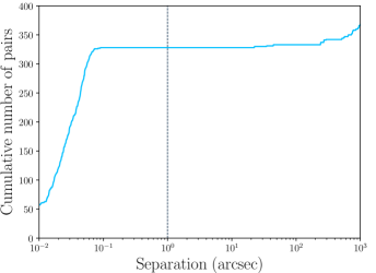
We combine all three sources into one dataset. There is a large cross-over between the Berger & Gies (2001) and BeSS datasets. We project each star onto the unit sphere and use those 3D positions to construct a $k$-dimensional tree. We call a duplicate any pair of stars in the combined dataset that are separated by less than $1\;\mathrm{arcsec}$. There are 328 pairs that meet this criterion. As Fig. 2 shows, there are no additional pairs in the range $1\mathrm{-}10\;\mathrm{arcsec}$ and thus there is no blurring between the duplicate population and the population of close stars that exist in binaries or dense clusters.

We find that three of the stars in our sample have unusually high radial velocities; CPD-32 2038 at $912.11\pm 97.922\;\mathrm{km}\;\mathrm{s}^{-1}$, HD 152979 at $-588.45\pm 51.38\;\mathrm{km}\;\mathrm{s}^{-1}$, and HD 165783 at $-507.353\pm 66.777\;\mathrm{km}\;\mathrm{s}^{-1}$. These velocities are from RAVE DR3 and DR4. In all three cases, the RAVE velocity measurements are the only ones that exist for these stars. Since all other stars in our sample have velocities $|v_{\mathrm{rad}}|<200\;\mathrm{km}\;\mathrm{s}^{-1}$, these are very likely to be spurious measurements. We remove all three stars from our sample. There are a further two stars, HD 306989 and CD-61 4751, whose only reported radial velocity from Reed (2003) has no associated radial velocity error and so these are also removed. This leaves us with a final sample of 632 stars. Their all-sky distribution in Galactic coordinates and median peculiar velocity distribution are shown in Figs. 3 and  4 respectively.

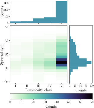
The Be star sample described above is a biased subset of all Be stars, partly due to the diversity of sources from which it has been drawn. The most significant bias is over-representation of early-type, giant stars, because our sample is flux-limited rather than volume-limited. We quantify this bias by using the spectral types and luminosity classes of the sample obtained from SIMBAD. Among the 632 stars, 599 have an associated spectral type and 532 also have a luminosity class. Multiple stars in the catalogue have a luminosity class of I or II, which contradicts the standard definition of a Be star and thus suggests that there is a degree of uncertainty in the luminosity classes. Similarly, there must be uncertainty in the stellar types because 38 stars are classified as Be stars but do not have a B spectral type. We choose to trust the Be star identification over the spectral type or luminosity class and thus include all 632 stars in our analyses in later sections.

We bin the stars in the two dimensional space of their spectral type $\{\mathrm{O}0,\mathrm{O}1,...,\mathrm{G}0\}$ and luminosity class $\{\mathrm{I},\mathrm{II},\mathrm{III},\mathrm{IV},\mathrm{V}\}$. Note that the spectral type or luminosity class can indicate a range of possible classifications. In this case, we divide up the contribution of that star to the histogram between all possible combinations of spectral type and luminosity class (i.e. a star whose classification was B1/2Iab/II would contribute a quarter to each of the bins B1I, B1II, B2I and B2II). We then apply a Kernel Density Estimation to this histogram with a bandwidth of 0.2322 (estimated using the rule of Scott, 2015 and assuming that each bin has unit length and width) which acts to smooth the histogram and reduce shot noise. This smoothed distribution is shown in Fig. 5. We make the assumption that this distribution adequately describes the selection function of the entire 632 stars. This assumption is well-motivated; the distribution of spectral types does not change significantly if we include the 67 stars which have spectral types, but not luminosity classes. Notably, Fig. 3 demonstrates that the stars which do not have these classifications are found preferentially in the Southern hemisphere, presumably due to an historical bias in the geographical distribution of telescopes. This bias further motivates the inclusion of all 632 stars in order to avoid spatial bias in our catalogue.

Figure 3: Distribution of Be stars in our combined catalogue across the sky. The size of each point is proportional to the parallax. The Galactic centre is at the centre of this image and the celestial equator is shown as a grey dashed line. A subset of the points are coloured orange to indicate stars which do not have an associated spectral type and luminosity class. Such stars are preferentially found in the Southern hemisphere.

Figure 4: Median peculiar velocity distribution of Be stars in our combined catalogue. Overplotted is a kernel density estimate.

Figure 5: Distribution of the 532 Be stars which have both spectral types and luminosity classes. The counts have been convolved with a Gaussian kernel of width 0.2322 to smooth out shot noise. There is a clear observational bias towards earlier types, while 38 stars are classified as Be stars but do not have a B spectral type.

3 The Post-Mass-Transfer Channel for Be Stars

The aim of this section is to use binary stellar population synthesis to predict the population properties of Be stars.

3.1 Be stars from binary population synthesis

Be stars produced through the post-mass-transfer route have interacted with their companion in the past. The runaway velocity is strongly dependent on their past evolution and is imprinted in their present day velocities. We model the evolution of binaries across a grid in parameter space using the binary_c population-nucleosynthesis framework  (Izzard et al., 2004, 2006, 2009). This code is based on the binary-star evolution (bse) algorithm of Hurley et al. (2002) expanded to incorporate nucleosynthesis, wind-Roche-lobe-overflow (Abate et al., 2013, 2015), stellar rotation (de Mink et al., 2013), accurate stellar lifetimes of massive stars (Schneider et al., 2014), dynamical effects from asymmetric supernovae (Tauris & Takens, 1998), an improved algorithm describing the rate of Roche-lobe overflow (Claeys et al., 2014), and core-collapse supernovae (Zapartas et al., 2017). In particular, we take our black hole remnant masses from Spera et al. (2015) and use a fit to the simulations of Liu et al. (2015) to determine the impulse imparted by the supernova ejecta on the companion. Grids of stars are modelled using the binary_grid2 module to explore the binary-star parameter space in primary mass $M_{1}$, secondary mass $M_{2}$ (or equivalently mass ratio $q$) and orbital period $P_{\mathrm{orb}}$. The grid variables have the ranges

$$1.0\leq M_{1}/M_{\sun} \leq 80.0,$$

$$0.1\;M_{\sun}/M_{1}\leq q \leq 1,$$ (1)

$$-1.0\leq\log_{10}(P_{\mathrm{orb}}/\mathrm{days}) \leq 10.0.$$

We assume the primary mass has the Kroupa (2001) IMF,

$$N(M_{1})\propto\begin{cases}M_{1}^{-0.3},&\mathrm{if}\ 0.01<M_{1}/M_{\sun}<0.08,\\ M_{1}^{-1.3},&\mathrm{if}\ 0.08<M_{1}/M_{\sun}<0.5,\\ M_{1}^{-2.3},&\mathrm{if}\ 0.5<M_{1}/M_{\sun}<80.0,\\ 0,&\mathrm{otherwise.}\end{cases}$$ (2)

We assume a flat mass-ratio distribution for each system over the range $0.1\;M_{\sun}/M_{1}<q<1$. We use the hybrid period distribution from Izzard et al. (2018) which gives the period distribution as a function of primary mass and bridges the log-normal distribution for low-mass stars (Duquennoy & Mayor, 1991) and a power law (Sana et al., 2012) distribution for OB-type stars. The grid is set at solar metallicity since Be stars have short lifetimes of less than $1\;\mathrm{Gyr}$, despite rejuvenation through mass-transfer extending the life of Be stars through the post-mass-transfer route by up to several $100\;\mathrm{Myr}$. binary_c has previously been used to consider the origins of Be stars by de Mink et al. (2013) in their investigation of the rotation rates of massive stars. They concluded that the 24.1% of their simulations that resulted in mass gain by the companion or a merger with the primary is consistent with the $20-30\%$ of early B type stars which are found to be Be stars (Zorec & Briot, 1997).

Be stars are dwarf or giant B type stars with emission-lines in the spectra. However, the atmospheres of stars are not modelled in detail by binary_c. We thus require a definition of a Be star based on the dynamic properties of the star. The natural expression is in terms of the ratio $R_{\mathrm{eq}}$ of the equatorial velocity $v_{\mathrm{eq}}$ to the critical equatorial velocity for break-up $v_{\mathrm{eq,crit}}$. Townsend et al. (2004) note that, while the canonical value for this ratio is $R_{\mathrm{eq}}\simeq 0.7-0.8$ based on measurements of the rotation of Be stars, this earlier work neglected the effect of equatorial gravity darkening. They postulate that this effect could lead to the Be star rotation rate being underestimated by tens of percent and that a value of $R_{\mathrm{eq}}\simeq 0.95$ is not ruled out. This near-critical rotation is in better agreement with the scenario first described by Struve (1931), in which material leaks out from the equator of a star spinning near breakup. To illustrate this point, Townsend et al. (2004) note that to launch material ballistically into orbit from the surface of a star spinning at $R_{\mathrm{eq}}\simeq 0.7$ requires an additional $100\;\mathrm{km}\;\mathrm{s}^{-1}$. Rivinius et al. (2013) reviewed the observational evidence and concluded that the minimum ratio for a B star to become a Be star is around 0.7 and that the lower limit of the mean ratio of the Be stars is around 0.8. For instance, Rivinius et al. (2006) found $R_{\mathrm{eq}}=0.75\pm 0.14$ as a lower limit without including gravity darkening. For this work, we consider the range $R_{\mathrm{eq}}\in(0,1)$ but focus on the set of plausible values $R_{\mathrm{eq}}\in\{0.65,0.75,0.85,0.95\}$. Based on the considerations above and results presented in Section 3.2, we choose the fiducial value $R_{\mathrm{eq}}=0.85$ to use in Section 4 onwards. The properties of the Be stars appear to be robust to the precise choice of $R_{\mathrm{eq}}$.

Another consideration is that, if a binary remains bound post-supernova, its centre of mass experiences a kick (Nelemans et al., 1999). This kick is not included at present in binary_c. However, Berger & Gies (2001) find that for a typical Be star scenario, the systematic kick is $8(\Delta M/\mathrm{M}_{\odot})\;\mathrm{km}\;\mathrm{s}^{-1}$ where $\Delta M$ is the mass lost by the primary in the supernova. They further note that this mass ratio is of order unity and thus that high velocity runaway binaries containing Be stars are not expected in general. In agreement with this theoretical expectation, observations of Be star - X-ray binaries in the Galaxy find that they have low peculiar velocities of $15\pm 6\;\mathrm{km}\;\mathrm{s}^{-1}$ (van den Heuvel et al., 2000), broadly similar to the velocity dispersions of a population of B stars containing no runaways (e.g. Aumer & Binney, 2009).

3.2 Properties of the simulated Be star population accounting for selection effects

The relationship between equatorial rotation and runaway velocity is central to understanding the post-mass-transfer model for the Be star phenomenon. First, mass transfer from the primary to the secondary shrinks the binary and accelerates the orbital velocity, and the orbital velocity is the principal contributor to the post-supernova runaway velocity. This mass transfer spins up the secondary, implying that high velocity runaways will also be rapidly rotating. Second, two massive stars in a close orbit tidally lock. This has the effect of breaking the relation between runaway velocity and rotation velocity for close binaries, which correspond to very fast runaways. This balance between mass transfer spinning up and tidal locking spinning down companions is demonstrated by a plot of runaway velocity $v_{\mathrm{run}}$ versus equatorial rotation velocity $v_{\mathrm{eq}}$ for all the simulated, runaway B stars (see Fig. 6), where there is a clear uptick in the equatorial velocity of the population over the range $30\lesssim v_{\mathrm{ej}}\lesssim 70\;\mathrm{km}\;\mathrm{s}^{-1}$. The structure of Fig. 6 is sensitive to the details of the binary evolution simulation, but in broad terms stars start on the left hand edge with a range of velocities. Some experience mass transfer from the primary which both spins them up and increases the orbit velocity. If the star is spun up to $v_{\mathrm{eq}}/v_{\mathrm{eq,crit}}>1$, then material is lost from the equator until it returns below the critical value. The star remains as a Be star unless mass transfer from the primary shrinks the orbit to the point where the timescale for tidal locking becomes short, in which case the star is spun down. Note that the separation, and hence runaway velocity, at which tidal locking becomes effective is a function of the masses of both components. This is the reason for the broad range of orbital velocities at which the companion is spun down.

Figure 6: Predicted probability distribution for the runaway velocity and critical equatorial velocity ratio of runaway B stars. The dashed line indicates our fiducial value $R_{\mathrm{eq}}=0.85$.

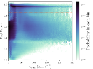
The predicted properties of Be stars discussed in the remainder of this section assume a steady-state in which there has been a constant star formation rate for longer than the age of the longest lived B star. The implication is that these distributions are predictions for the observable population rather than the stars produced in a single starburst. At each timestep of the binary evolution, we check whether either component of the binary is a B star. If so, we tabulate both the properties of the binary and the probabilistic weight of the system given by the length of the timestep $\mathrm{d}t$ multiplied by the probability of the progenitor binary $\operatorname{P}(M_{1},q,P_{\mathrm{orb}})$.

The frequency of Be stars among the simulated B stars monotonically depends on our choice of $R_{\mathrm{eq}}$. Across spectral types B0-B9 and luminosity classes V-III, we find that the frequency of Be stars is 7.9% for $R_{\mathrm{eq}}=0.65$ and declines to 1.9% for $R_{\mathrm{eq}}=0.95$. These frequencies are lower than are observed (e.g. Zorec & Briot, 1997). However, these predicted frequencies are sensitive to uncertain prescriptions for the birth rotation velocities and rotational evolution of the simulated stars. For instance, the birth rotation velocities in the fiducial model are given by an empirically-derived formula from Hurley et al. (2000). If this prescription under-predicts the birth rotation velocities, then this will lead to a lower frequency of Be stars. We investigate this by setting the birth rotation velocity of each star to be the critical rotation velocity. In this extreme case, we find a Be star frequency of 81.7% for $R_{\mathrm{eq}}=0.65$ which declines to 3.3% for $R_{\mathrm{eq}}=0.95$. Based on considerations in the previous section, a value $R_{\mathrm{eq}}=0.85$ seems most plausible, in which case our fiducial model gives a frequency of 3.1% while the extreme model gives 25.5%. These numbers bracket the observed frequency of Be stars and thus we conclude that an adjustment to the prescriptions for the birth rotation velocities and rotational evolution could bring our prediction in line with observations. While the extreme model boosts the abundance of Be stars by making an unphysical assumption, it does not substantially alter the properties of the resulting Be star population. Thus the predictions made for the properties of Be stars are robust to the adjustments necessary to replicate the observed Be star frequency.

Mass transfer can spin the companion up and cause the Be star phenomenon, but it also decreases the orbital separation and thus increases the velocity of the subsequent runaway Be star. One consequence is that, in rough terms, the longer the mass transfer continues, the more rapidly rotating the companion star and the faster the runaway velocity, implying that the frequency and velocity distribution of runaway stars amongst the Be star population depend on $R_{\mathrm{eq}}$. Additionally, the distribution of runaway star velocities is conditional on the mass of the star (for instance, see Fig. 2 in Boubert et al., 2017) and this should hold for Be stars. An observable proxy for mass is the spectral type of the star and thus we can re-phrase the velocity distributions as being conditional on the spectral type. However, we established in Section 2 that our catalogue of Be stars is biased towards early-type Be stars. The implication is that the prediction for the runaway frequency and velocity distribution of the Be stars obtained through simulation is not directly comparable with our Be star catalogue. We account for this selection bias by re-weighting the simulated Be star population to match the observed luminosity class and spectral type distribution. Note that each choice of $R_{\mathrm{eq}}$ defines a different Be star population, and thus the re-weighting is carried out for each value of this parameter.

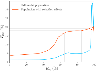
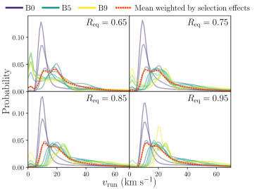
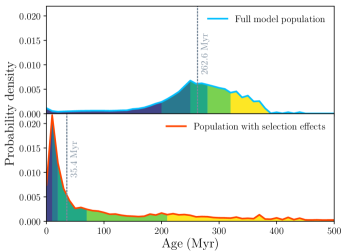
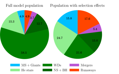
Weighting the simulation outcomes by the observed luminosity class and spectral type distribution has a large effect both on the runaway star sub-population (Fig. 7) and on the Be star population in general (Fig. 8). We refer to our Be star population from the synthesis as our full model population, while that with all known selection effects included will be referred to as the model population with selection effects.

1. The predicted frequency of runaway stars amongst the model Be star population is increased, as shown in Fig. 7(a). Earlier stellar types tend to have a greater runaway fraction (e.g. Blaauw, 1961) and the re-weighting increases the weight given to early-type Be stars. Fig. 7(a) shows that choices of larger $R_{\mathrm{eq}}$ are correlated with greater runaway fractions. One possible reason is that stars which are closer to critical-rotation have experienced more mass-transfer, and thus tend to have a more massive partner whose core-collapse supernova would more easily disrupt the binary.

2. The re-weighting alters the predicted runaway velocity distribution by increasing the contribution of early-type Be stars (Fig. 7(b)). Interestingly, the mean accounting for selection effects is almost independent of the choice of $R_{\mathrm{eq}}$, making this mean robust to our fiducial choice of $R_{\mathrm{eq}}=0.85$.

3. Under the assumption of $R_{\mathrm{eq}}=0.85$, the median Be star age drops from $261.7\;\mathrm{Myr}$ to $35.4\;\mathrm{Myr}$ (Fig. 8(a)). The drastic difference can be explained by the steepness of the mass-main sequence lifetime relation $\tau_{\mathrm{MS}}\propto M^{-2.5}$ (e.g. Hansen et al., 2004).

4. Pols et al. (1991) point out that the majority of Be stars formed through the post-mass-transfer scenario are still bound to their companion, because the primary normally transfers sufficient mass to the secondary to either avoid the supernova or for the reduced mass loss in the supernova to not unbind the system. These companions are white dwarfs, neutron stars and black holes. The re-weighting changes both the fraction of the observed Be star population predicted to be in binaries and the stellar types of those companions (Fig. 8(b)). Assuming $R_{\mathrm{eq}}=0.85$, our simulation predicts that more than 90% of all Be stars are in binaries, but that among our observed sample only 77.1% are in binaries. Furthermore, the observed binaries are less than half as likely to contain a Be star with a white dwarf companion. The companion that transfers mass to form the Be star must be low-mass in order for the remnant to be a white dwarf, thus the companion Be star must itself be low-mass and so late-type. The high fraction of Be stars residing in binaries with neutron stars or black holes agrees qualitatively with observations of high mass X-ray binaries (HMXBs) in the Magellanic Clouds. In fact, 33 of the 40 HMXBs in the Large Magellanic Cloud (Antoniou & Zezas, 2016) and 69 of the 70 HMXBs in the Small Magellanic Cloud (Antoniou & Zezas, 2016) have Be star companions. Curiously, these authors note that the star formation efficiency of HMXBs in the Large Magellanic Cloud is 17 times smaller than in the Small Magellanic Cloud and argue that this is due to the difference in age and metallicity of the two stellar populations. The effect of varying metallicity on our predictions is an interesting avenue for future work.

(a) Runaway fraction as a function of $R_{\mathrm{eq}}$

(b) Velocity distribution of the runaway Be stars as a function of $R_{\mathrm{eq}}$

Figure 7: Both selection effects and the uncertainty in the choice of $R_{\mathrm{eq}}$ (the minimum fraction of the critical rotation velocity for a star to be classed as a Be star) can lead to dramatically different simulated populations of runaway Be stars. Top: The runaway fraction among Be stars as a function of $R_{\mathrm{eq}}$ with and without accounting for the observational selection effect. The grey lines indicate the resulting runaway fraction associated with each choice of $R_{\mathrm{eq}}$ shown in the lower panel. Bottom: The choice of $R_{\mathrm{eq}}$ changes the velocity distribution of the runaway Be stars as a function of spectral type. In each panel, we show the velocity distribution for each spectral type from B0 to B9, in addition to the mean accounting for the selection effect. Note that as $R_{\mathrm{eq}}$ increases the effect of Poisson noise also increases because we are defining fewer stars to be Be stars.

(a) Age distribution of the simulated Be stars

(b) % of Be stars where the binary is intact, merged or split

Figure 8: The inclusion of observational biases dramatically changes the predicted population of Be stars, under the assumption of $R_{\mathrm{eq}}=0.85$. Top: The two panels show the distribution of ages of the Be stars with and without accounting for the observational bias towards early-type Be stars. The grey dashed lines indicate the median age and the coloured regions each account for 20% of the probability. Bottom: Each pie chart gives the proportions of the Be stars for which the progenitor binary is intact, merged or split. If the binary is intact then the stellar type of the companion is given. MS = Main Sequence, WDs = White Dwarf, NS = Neutron Star, BH = Black Hole.

An important aspect of this work is that binary_c does not carry out full stellar structure integration, instead opting for prescriptions that permit the rapid evolution of a large number of binary stars. This simplification allows for rapid population synthesis studies and places binary_c in the class of synthetic binary stellar evolution codes (see Table 2 of De Marco & Izzard, 2017 for a list of synthetic and detailed binary stellar evolution codes). Similar studies to the present one have been carried out with detailed binary stellar evolution codes, for instance by van Rensbergen et al. (1996) and more recently by Eldridge et al. (2011).

3.3 Compact object natal kick uncertainty

There are several aspects of binary stellar physics that are poorly constrained observationally and must be prescribed when doing population synthesis. Three examples of relevance to the study of runaway stars are common envelope evolution, natal kicks of compact objects and fallback of material onto black holes. We attempt to quantify how different prescriptions alter our results by generating a population of binary stars with each prescription. However, common envelope evolution is sufficiently poorly understood that there are whole families of alternative prescriptions, so that an investigation of this uncertainty is beyond the scope of this paper. In contrast, for natal compact object kicks, we need only define the probability distribution of kicks $\operatorname{P}(v_{\mathrm{kick}})$. There are several distributions in the literature that are fits of analytic models to data. We show a sample of the most popular distributions in Fig. 9, including our fiducial choice of the Maxwellian distribution from Hansen & Phinney (1997). Clearly, the true natal kick distribution is not known at present – even fits within the same work giving radically different distributions (i.e. Faucher-Giguère & Kaspi, 2006)! A distribution with a large number of low-velocity compact objects predicts a high fraction of runaways with compact companions.

Figure 9: Various distributions for the 3D natal kick velocity distribution of neutron stars from the literature. The solid lines are the single Maxwellian distributions of Hansen & Phinney (1997) and Hobbs et al. (2005), the dash-dotted lines are from Hartman (1997) and Faucher-Giguère & Kaspi (2006), and the dashed lines are the double Maxwellian distributions of Arzoumanian et al. (2002) and Faucher-Giguère & Kaspi (2006).

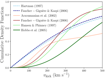
To explore the impact of the choice of distribution, we simulate a population of binary stars using the Hartman (1997) distribution. This distribution has about 20% of neutron stars receiving a kick less than $100\;\mathrm{km}\;\mathrm{s}^{-1}$ and thus we expect more binaries to survive the supernova of the primary. The most direct outcome of switching to the Hartman (1997) prescription is that in the full model population, 0.6% fewer Be stars are runaways and 0.6% more are in binaries with neutron stars or black holes. In the population with selection effects included, this trend still holds true, with 15.3% Be star runaways and 17.6% Be stars in compact object binaries. Another trend is a slight move in the runaway velocity distribution to slower velocities by roughly $0.5\;\mathrm{km}\;\mathrm{s}^{-1}$, which is a consequence of both the slower speeds of the neutron stars and the fact that energy is proportional to velocity squared. Even if two objects are unbound they still lose speed while escaping, and the speed lost is greater if the two objects have a smaller relative velocity.

Fallback of material onto a black hole in the seconds after the supernova can damp the birth kick and potentially lead to binaries surviving supernovae. One prescription for this fallback was presented in Fryer et al. (2012), who noted that it can alter the predicted number of $2-5\;\mathrm{M}_{\odot}$ black holes in X-ray binaries by tens of percent (Be stars are frequently found in X-ray binaries). We have not included this fallback in our fiducial model because the uncertainty inherent in the fallback prescription couples to the uncertainty in both the mass of the compact remnant after a supernova (i.e. whether the remnant is a neutron star or a black hole) and the natal kick distribution. Exploring the full space of possible prescriptions is beyond the scope of this paper. However, we believe that including fallback should cause a change in the Be star runaway fraction comparable to changing the natal kick distribution to that of Hartman (1997).

We conclude that the uncertainty in the distribution of natal kicks of compact objects does not greatly impact our results, aside from decreasing the expected Be star runaway fraction by a few percent. One reason for the small scale of the change is that whether a binary is disrupted by a supernova is principally determined by whether the primary loses more than half its mass (Blaauw, 1961), and the kick on the compact object is only a second order effect. The uncertainty in the fallback of material onto a black hole remnant could couple with the natal kick uncertainty, however, and the Be star runaway fraction predicted for the observed catalogue could be as low as 10%.

4 Bayesian Framework

We now ask what fraction of the observed Be stars are runaway stars, which is closely related to the question of what fraction can have their origins with the post-mass-transfer model. This is a more subtle question than simply looking for Be stars with peculiar velocities greater than $40\;\mathrm{km}\;\mathrm{s}^{-1}$, as done by Berger & Gies (2001), because Fig. 7(b) shows that the median runaway velocity of our simulated Be runaway stars (accounting for observational biases) is only $19.6\;\mathrm{km}\;\mathrm{s}^{-1}$. Aumer & Binney (2009) used Hipparcos astrometry and photometry and Geneva-Copenhagen radial velocities to calculate the velocity dispersion as a function of colour of 15,000 nearby main-sequence and subgiant stars. For blue stars $B-V<0$, they find that the total velocity dispersion is less than $20\;\mathrm{km}\;\mathrm{s}^{-1}$. We would thus expect only a small fraction of Be star runaways to have a peculiar velocity in excess of $40\;\mathrm{km}\;\mathrm{s}^{-1}$. Another factor is that, in the post-mass-transfer scenario, most Be star producing binaries either evade the supernova through mass transfer or remain bound post-supernova. Thus, most Be stars are found in binaries with white dwarfs, neutron stars or black holes (Fig. 8(b)). This means that only a few percent of all Be stars need have peculiar velocities in excess of $40\;\mathrm{km}\;\mathrm{s}^{-1}$ in order to imply that all Be stars are produced through the post-mass-transfer channel.

4.1 Bayesian Mixture Model for the Kinematics

The null hypothesis for a young star in the Milky Way disc is that the velocity is well described by the disk rotation plus velocities drawn from a velocity ellipsoid centred on zero with dispersions $(\sigma_{\mathrm{R}},\sigma_{\phi},\sigma_{\mathrm{z}})$. The velocity dispersions increase with the age on timescales of the order of $1\;\mathrm{Gyr}$. We can reasonably neglect the age dependency and thus assume the dispersions are constant.

We construct a model for a population of stars in the thin disc built from three sub-populations. A fraction $F_{\mathrm{disc}}$ are well-described by the null hypothesis, a fraction $F_{\mathrm{run}}$ are runaways and have an additional randomly oriented velocity $v_{\mathrm{run}}$, and a fraction $F_{\mathrm{out}}$ are outliers and have a different randomly oriented velocity $v_{\mathrm{out}}$. One physical interpretation of any outliers is that they are stars that have under-gone the two-step-ejection scenario of Pflamm-Altenburg & Kroupa (2010), in which a massive binary is ejected from a cluster by a dynamical interaction and the companion is later accelerated a second time by the supernova of the primary. There are only two free parameters that describe these fractions because they sum to unity and so form a simplex. We assume that every point in this simplex is equally likely, which can be implemented as a flat Dirichlet prior. The probability of observing a star with observables $\boldsymbol{x}$ under this composite model is simply a linear combination of the three probability density functions,

$$P(\boldsymbol{x})=F_{\mathrm{disc}}P(\boldsymbol{x}\lvert\mathrm{disc})+F_{\mathrm{run}}P(\boldsymbol{x}\lvert\mathrm{runaway})+F_{\mathrm{out}}P(\boldsymbol{x}\lvert\mathrm{outlier}).$$ (3)

The motivation for including an outlier population is that in Sec. 2.4, we removed three stars which had obviously erroneous radial velocities $|v_{\mathrm{rad}}|>500\;\mathrm{km}\;\mathrm{s}^{-1}$. However, some spuriously large velocities may remain and boost the inferred runaway fraction. The functions $P(\boldsymbol{x}\lvert\mathrm{model})$ are the priors for the model parameters multiplied by the likelihood of the data with those model parameters.

The observable properties of each star are the parallax $\omega$, proper motions $(\mu_{\alpha\ast},\mu_{\delta})$ and radial velocity $v_{\mathrm{rad}}$. The quantities we have are imperfect measurements of the true parallax $\tilde{\omega}$, the true proper motions $(\tilde{\mu}_{\alpha\ast},\tilde{\mu}_{\delta})$ and the true radial velocity $\tilde{v}_{\mathrm{rad}}$. The true heliocentric distance $\tilde{d}$ is then $1/\tilde{\omega}$ and, independently, the true Galactocentric velocities $(\tilde{v}_{\mathrm{R}},\tilde{v}_{\phi},\tilde{v}_{\mathrm{z}})$ can be found using the equations in Johnson & Soderblom (1987). Both these transforms are bijective, thus we are free to express our model in either the distance or parallax and with either of the sets of the velocities. Note that the bijectivity is conditional on the other nuisance parameters having been fixed, such as the Solar position $R_{\odot}$. Theoretically, the choice does not change the result of the Bayesian inference and only switches our priors and likelihoods. However, for practical reasons discussed later, it is advantageous to pick the parameters which give the tightest prior. We choose to express our prior in the parameters $(\tilde{d},\tilde{\mu}_{\alpha\ast},\tilde{\mu}_{\delta},\tilde{v}_{\mathrm{rad}})$ and thus the likelihood in the parameters $(\tilde{\omega},\tilde{v}_{\mathrm{R}},\tilde{v}_{\phi},\tilde{v}_{\mathrm{z}})$. We include the necessary Jacobian $k^{2}$, where $k\approx 4.74057$ is the conversion factor between $\mathrm{AU}\;\mathrm{yr}^{-1}$ and $\mathrm{km}\;\mathrm{s}^{-1}$.

4.2 The Priors

Consider a model that has parameters $\boldsymbol{\theta}$ that makes a prediction for some observable data $\boldsymbol{x}$. If we have a function $\operatorname{Prior}(\boldsymbol{\theta})$ that describes our prior expectation of the values that the parameters can take and a function $\operatorname{Likelihood}(\boldsymbol{x}\lvert\boldsymbol{\theta})$ that says how likely the data $\boldsymbol{x}$ is given a specific choice of the parameters, then our posterior knowledge of the parameters after measuring the data is specified through the distribution

$$\operatorname{Posterior}(\boldsymbol{\theta}\lvert\boldsymbol{x})\propto\operatorname{Prior}(\boldsymbol{\theta})\operatorname{Likelihood}(\boldsymbol{x}\lvert\boldsymbol{\theta}).$$ (4)

If new data are subsequently taken, then this posterior distribution should be used as the prior when incorporating the new data. Through this iterative process our knowledge of the parameters converges on their true values.

The parameters can be split into global parameters $\boldsymbol{\theta}^{\mathrm{g}}$ of the entire population and local parameters $\boldsymbol{\theta}^{\mathrm{l}}$ of each star. The global parameters only appear once in the prior. However, if the model is applied to $N$ stars then $N$ independent copies of the local parameters must be included and are labelled as $\boldsymbol{\theta}^{i}$.

4.2.1 Global Parameters

The peculiar velocity of the population at birth is assumed to be Gaussian in each of the radial, azimuthal and vertical directions, centred on zero and with independent dispersions $(\sigma_{\mathrm{R}},\sigma_{\phi},\sigma_{\mathrm{z}})$. We place a weakly informative Gaussian prior centred on $10\;\mathrm{km}\;\mathrm{s}^{-1}$, with a $10\;\mathrm{km}\;\mathrm{s}^{-1}$ dispersion and bounded below at zero on each of these dispersions. An additional hyper-parameter is the characteristic length-scale $L$ of the population, for which we assume a weakly informative Gaussian prior centred on $0.5\;\mathrm{kpc}$, with a $0.5\;\mathrm{kpc}$ dispersion and bounded below at zero. Astraatmadja & Bailer-Jones (2016) found $L\approx 1.35$ for a simulation of the contents of the full Gaia catalogue and thus the prior of $L$ was motivated by the lower magnitude limit of TGAS. There are five nuisance parameters whose priors are Gaussians centred on their measured value and with a dispersion given by the measurement error: the rotation of the Galactic disc $V_{\mathrm{c}}$, the Galactocentric radius of the Sun $R_{\odot}$, and the peculiar velocities of the Sun $(U_{\odot},V_{\odot},W_{\odot})$. We assume that the Milky Way disc rotates with a flat circular velocity of $V_{\mathrm{c}}=238\pm 9\;\mathrm{km}\;\mathrm{s}^{-1}$ and that the Sun orbits at the Galactocentric radius $R_{\odot}=8.27\pm 0.29\;\mathrm{kpc}$ with a peculiar velocity $(U_{\odot},V_{\odot},W_{\odot})=(11.1\pm 0.75\pm 1,12.24\pm 0.47\pm 2,7.25\pm 0.37\pm 0.5)\;\mathrm{km}\;\mathrm{s}^{-1}$ (Schönrich et al., 2010; Schönrich, 2012).

4.2.2 Local Parameters

For the true heliocentric distance $\tilde{d}$, we use the exponentially decreasing volume density prior of Bailer-Jones (2015)

$$P(\tilde{d})=\begin{cases}\frac{\displaystyle\tilde{d}^{2}}{\displaystyle 2L^{3}}\exp\left(-\tilde{d}/L\right),&\text{if}\ \tilde{d}>0,\\ \hbox{}&\hbox{}\textstyle\\ 0,&\text{otherwise},\end{cases}$$ (5)

where $L$ is the characteristic length scale hyper-parameter. We remark that this can be equivalently stated in terms of the Gamma distribution as $\mathrm{Gamma}(3,L)$. For the true proper motions and radial velocity, the prior is a Gaussian centred on the measured value and with a dispersion given by the measurement error. Both the runaway and outlier populations have an additional velocity described by a speed and a unit vector. The unit vector of ejection $\boldsymbol{x}_{\mathrm{ej}}$ is assumed to be uniformly distributed on the unit sphere. The runaway speed $v_{\mathrm{run}}$ is drawn from the analytic distribution obtained in Sec. 4.4. The outlier speed $v_{\mathrm{out}}$ is drawn from a Gaussian centred on zero and with a $500\;\mathrm{km}\;\mathrm{s}^{-1}$ dispersion. Both speeds are constrained to be greater than zero.

In summary, the prior is

$$\operatorname{Prior}(\boldsymbol{\theta})=\operatorname{Global}(\boldsymbol{\theta}^{\mathrm{g}})\prod_{i}\operatorname{Local}(\boldsymbol{\theta}^{i}),$$ (6)

where

$$\operatorname{Global}(\boldsymbol{\theta}^{\mathrm{g}})= \operatorname{Simplex}(F_{\mathrm{disc}},F_{\mathrm{run}},F_{\mathrm{out}})\operatorname{Normal}(\sigma_{\mathrm{R}},\sigma_{\phi},\sigma_{\mathrm{z}})$$

$$\times\operatorname{Normal}(L)\operatorname{Normal}(V_{\mathrm{c}},R_{\odot},U_{\odot},V_{\odot},W_{\odot}),$$ (7)

and

$$\operatorname{Local}(\boldsymbol{\theta}^{\mathrm{l}})= \operatorname{Gamma}(\tilde{d})\operatorname{Normal}(\tilde{\mu}_{\alpha\ast},\tilde{\mu}_{\delta},\tilde{v}_{\mathrm{rad}})$$

$$\times\operatorname{DLN}(v_{\mathrm{run}})\operatorname{Normal}(v_{\mathrm{out}})\operatorname{UnitVector}(\boldsymbol{x}_{\mathrm{ej}}).$$ (8)

All parameters except the fractions $(F_{\mathrm{disc}},F_{\mathrm{run}},F_{\mathrm{out}})$ and the three components of the unit vector $\boldsymbol{x}_{\mathrm{ej}}$ are independent and the groupings have only been made to simplify the notation. The function $\operatorname{DLN}(\cdot)$ indicates the double log-normal fit to the numerical runaway velocity distribution discussed in Sec. 4.4.

4.3 The Likelihood

The likelihood gives the probability of observing the data $\boldsymbol{x}$ given the model parameters $\boldsymbol{\theta}$. Note that in this problem the data can be broken down into a set of local data $\boldsymbol{x}^{\mathrm{l}}$ for each star whose likelihood only depends on the global parameters $\boldsymbol{\theta}^{\mathrm{g}}$ and the local parameters $\boldsymbol{\theta}^{\mathrm{l}}$ of that star. Continuing the notation above, we use $\boldsymbol{x}^{i}$ and $\boldsymbol{\theta}^{i}$ to label the local data and parameters of a specific star $i$. The likelihood is the product of the likelihoods of each star with each individual likelihood containing four terms. The first states how likely the observed parallax $\omega$ is given the true parallax $\tilde{\omega}$ and is a Gaussian centred on the true parallax with the measurement error on the parallax as the dispersion. The remaining three terms give the likelihood of the peculiar velocity and are Gaussians centred on zero and with dispersions given by the parameters $(\sigma_{\mathrm{R}},\sigma_{\phi},\sigma_{\mathrm{z}})$. In summary the likelihood is,

$$\operatorname{Likelihood}(\boldsymbol{x}\lvert\boldsymbol{\theta})=\prod_{i}\operatorname{Likelihood}(\boldsymbol{x}^{i}\lvert\boldsymbol{\theta}^{\mathrm{g}},\boldsymbol{\theta}^{i}),$$ (9)

where

$$\operatorname{Likelihood}(\boldsymbol{x}^{\mathrm{l}}\lvert\boldsymbol{\theta}^{\mathrm{g}},\boldsymbol{\theta}^{\mathrm{l}}) =k^{2}\operatorname{Normal}(\omega)\left[F_{\mathrm{disc}}\operatorname{Normal}(\tilde{v}_{\mathrm{R}},\tilde{v}_{\phi},\tilde{v}_{\mathrm{z}})\right.$$

$$\left.+F_{\mathrm{run}}\operatorname{Normal}(\tilde{v}_{\mathrm{R}}-v_{\mathrm{run,R}},\tilde{v}_{\phi}-v_{\mathrm{run,}\phi},\tilde{v}_{\mathrm{z}}-v_{\mathrm{run,z}})\right.$$

$$\left.+F_{\mathrm{out}}\operatorname{Normal}(\tilde{v}_{\mathrm{R}}-v_{\mathrm{out,R}},\tilde{v}_{\phi}-v_{\mathrm{out,}\phi},\tilde{v}_{\mathrm{z}}-v_{\mathrm{out,z}})\right].$$ (10)

The groupings are only made to simplify the notation and the $k^{2}$ is the Jacobian of the transformation.

4.4 Analytic Fit to Runaway Velocity Distributions

The final ingredient that we need before application of Hamiltonian Monte Carlo techniques is an analytic fit to the numerical distribution of simulated runaway velocities from Sec. 3. We specifically refer to the runaway velocity distribution for the model Be star population defined by $R_{\mathrm{eq}}=0.85$ accounting for the observational selection effect, after averaging across the different stellar types. This step is necessary as the derivatives of the posterior with respect to the parameters need to be calculable.

We opt to use the log-normal distribution, defined by the probability density function,

$$\mathrm{P}(x\;|\;\mu,\sigma)=\begin{cases}\frac{\displaystyle 1}{\displaystyle x\sigma\sqrt{2\pi}}\exp\left(-\frac{\displaystyle\left(\ln x-\mu\right)^{2}}{\displaystyle 2\sigma^{2}}\right),&\mathrm{if}\;x>0,\\ \hbox{}&\hbox{}\textstyle\\ 0,&\mathrm{otherwise},\end{cases}$$ (11)

and with cumulative density function,

$$\mathrm{F}(x\;|\;\mu,\sigma)=\begin{cases}\frac{1}{2}+\frac{1}{2}\operatorname{erf}\Big{[}\frac{\displaystyle\ln x-\mu}{\displaystyle\sqrt{2}\sigma}\Big{]},&\mathrm{if}\;x>0,\\ 0,&\mathrm{otherwise}.\end{cases}$$ (12)

The log-normal distribution has several properties which make it appropriate for modelling a runaway velocity distribution:

1. log-normals are constrained to be non-zero only for positive $x$,

2. the mode is given by

   $$\exp{\left(\mu-\sigma^{2}\right)}$$

   and thus for $\mu<<\sigma^{2}$ a log-normal can approximate a decay,

3. the skewness is given by

   $$\left(\exp{\sigma^{2}}+2\right)\sqrt{\vphantom{\sum}\exp{\sigma^{2}}-1}$$

   and so for small $\sigma$ a log-normal can be used to approximate a symmetric distribution offset from the origin.

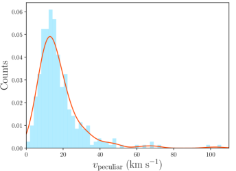
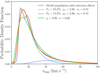
We fit a mixture of two log-normal distributions to the numeric runaway velocity distribution using the implementation of non-linear least squares in SciPy. We found that the fit was best performed using the cumulative density function. In Fig. 10 we show a comparison between the probability density functions of our numeric distribution compared to the sum of the two log-normal distributions, as well as a fit containing a single log-normal distribution to illustrate the improvement. The double log-normal does not capture the bimodality near the peak of the distribution, but does trace the tail to large velocities.

Figure 10: Fits of one and two log-normal distributions to the numerical predicted runaway velocity distribution calculated in Section 3. In the legend, the $\mu$ and $\sigma$ give the parameters of each log-normal distribution and $F_{1}$ and $F_{2}$ are the fraction of the probability assigned to each component of the double log-normal fit.

5 The Fraction of Be Runaways

5.1 Preliminaries

363 of the 632 stars in our observed sample have TGAS astrometry and thus have a published covariance matrix between their position, parallax and proper motions. We neglect the covariance matrix here, but plan to revisit the problem after the second Gaia data release, which will include the vast majority of the known Be stars. Positions in TGAS are measured with $\mathrm{milliarcsecond}$ accuracy which at a distance of $1\;\mathrm{kpc}$ corresponds to a spatial accuracy of $5\;\mu\mathrm{pc}$. The distance over which the properties of the Galaxy vary is much larger than this and thus we fix the position of each star.

Note that, in principle, we could condition the runaway velocity distribution for individual Be stars on their stellar type. However, there are two main arguments against this. First, the individual runaway velocity distributions are subject to greater Poisson noise than their weighted mean. Second, the spectral types for the Be stars in our sample were queried from SIMBAD and thus have a variety of provenances. Taken as a whole, they likely give a good summary of the spectral type distribution of the sample. However, each individual spectral type has a different and unknown uncertainty. If the sample had measured effective temperatures and luminosities with uncertainties, then it would be sensible to condition the runaway velocity distribution of individual Be stars on these physical properties. Such an approach will become viable with the second Gaia data release.

When our model is applied to the 632 stars in our observed Be star database, we have 5067 free parameters. These are broken down into eleven global parameters which describe the entire sample and eight local parameters for each star. We used the Bayesian inference platform Stan (Carpenter et al., 2017), accessed through CmdStan, to obtain the posterior for the model. Stan includes a Hamiltonian Markov chain Monte Carlo sampler which incorporates No-U-Turn Sampling (Hoffman & Gelman, 2011) and so is well suited to high-dimensional problems. We ran four chains and computed the potential scale reduction statistic $\hat{R}$ (Gelman & Rubin, 1992) across the chains to assess convergence. We used an equal number of warm-up and sampling iterations and doubled the number of iterations until the model converged. The four chains were then merged and used to calculate the statistics.

5.2 Retrieval of simulated data

A minimum requirement of a successful Bayesian model is the ability to retrieve the input model parameters of simulated data. This is equivalent to saying that if our model of Be star kinematics is correct and complete, then the parameters we retrieve should be close to the true values. One common reason for this not to be true is the existence of a degeneracy between two parameters which the data are not precise enough to break. For our Be star model, we expect there to be a strong degeneracy between the three velocity dispersions and the runaway fraction, and thus it is essential that we investigate whether the uncertainties on our data are sufficiently small to allow this degeneracy to be broken.

We generate a test set of stars assuming known $F_{\mathrm{run}}=17.5\%$ and $(v_{\mathrm{R}},v_{\phi},v_{\mathrm{z}})=(12,10,4)\;\mathrm{km}\;\mathrm{s}^{-1}$. We draw a random set of $(V_{\mathrm{c}},R_{\odot},U_{\odot},V_{\odot},W_{\odot})$ from within their uncertainties to act as the ‘truth’ of the fake catalogue. We create the fake stars in a one-to-one correspondence with the real catalogue, taking both the positions and uncertainties from the true stars. The size of the uncertainties roughly correlates with the distance to the star, so to sample a realistic distance to each fake star given the uncertainties, we draw from the posterior for the distance to the real star $\operatorname{Gamma}(0,L)\operatorname{Normal}(\omega,\sigma_{\omega})$, where we fix $L=0.2\;\mathrm{kpc}$ and $(\omega,\sigma_{\omega})$ refer to the parallax and uncertainty of the real star. To generate the radial velocities and proper motions, we first draw three random velocities from the velocity dispersion distributions, add on a randomly oriented ejection velocity for the randomly selected subset of runaway stars, and then transform to the equatorial frame. Finally, the parallaxes, radial velocities and proper motions are convolved with the uncertainties. Note that we do not include an outlier population.

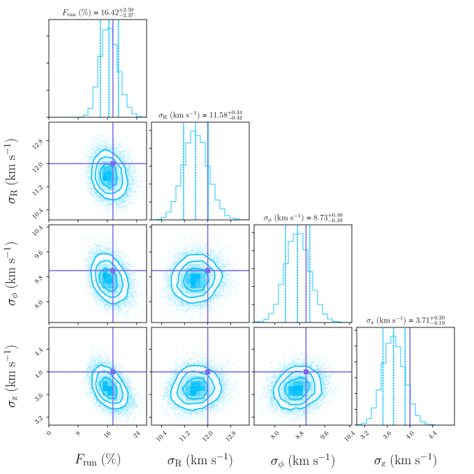
Our principal model is the one introduced in Sec. 4, which has contributions from disk, outlier and runaway populations and which uses the double log-normal fit to the runaway velocity distribution. We present the posterior for this model when applied to the fake catalogue in Fig. 11, with the true values shown in purple. The interpretation of this plot is that the uncertainties on the current set of Be stars are too large to wholly break the degeneracy between $F_{\mathrm{run}}$ and the velocity dispersions. However, given the width of the priors on these parameters, the retrieved values are remarkably in agreement with the true values.

Figure 11: Corner plot of the posterior for the retrieval.

While our chief concern is the runaway fraction among the entire Be star population, it is interesting to consider whether our method is successful at classifying individual stars. We expect that stars are only successfully classified as runaways if they are travelling sufficiently rapidly, but not so rapidly as to be misclassified as outliers. Our method does not classify stars directly, but does return the probability of membership of each class. An obvious classification scheme is that if the probability of being a runaway star is greater than $x\%$, then the star is classed as a runaway. One common metric to decide what value of $x$ to use is the receiver operating characteristic curve (Fig. 12), where the true positive rate and false positive rate are plotted as a parametric function of $x$. A classification scheme where any star with a probability of being a runaway star greater than 50% is classed as a runaway star performs well, because it can pick out more than half the true runaway stars with only 10% contamination.

Figure 12: The receiver operating characteristic curve for the classification of runaway stars based on the mean of the posterior probability of being a runaway star being greater than $x\%$. The grey dashed line corresponds to a classifier that randomly guesses and which our classification far out-competes. The annotations are of the form ‘$x\%\Rightarrow(\#\;\mathrm{of}\;\mathrm{True}\;\mathrm{Positives},\#\;\mathrm{of}\;\mathrm{False}\;\mathrm{Positives})$’.

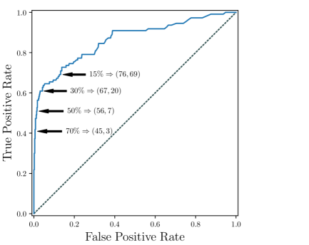
We conclude both that our method can accurately retrieve the fraction of runaway stars and the velocity dispersions, as well as produce a low-contamination list of runaway stars.

5.3 Principal model

Figure 13: Corner plot of the posterior for the principal model.

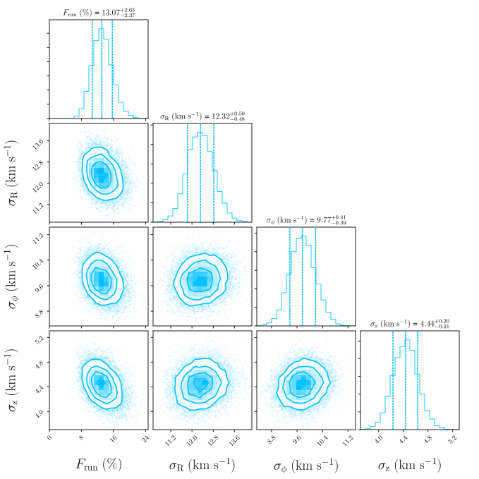
We now apply the model to the true catalogue of Be stars described in Section 2. In Fig. 13, we show the posterior for the runaway fraction $F_{\mathrm{run}}$ and the velocity dispersions of the population. The outlier fraction is only $F_{\mathrm{out}}=0.36\begin{subarray}{c}+0.35\\ -0.22\end{subarray}\%$ which means that the high velocity stars are sufficiently well described by the runaway model. The posterior runaway fraction is about $13.1^{+2.6}_{-2.4}\%$. Using the classification scheme from Sec. 5.2, 40 stars are classified as runaway stars and they are given in Table 1. 7 of these stars were classed as high peculiar space velocity stars by Berger & Gies (2001) and this subset are indicated in Table 1. We perform a brief search of SIMBAD to look for particularly interesting cases:

• Menkib: There are only 313 IAU-approved named stars and thus the appearance of one in a modern astronomical paper is remarkable. Menkib is a previously known runaway star (Hoogerwerf et al., 2001) in the constellation of Perseus and associated with the $2.5^{\circ}$ bowshock nebula NGC 1499 (otherwise known as the California Nebula).

• Eclipsing binaries: W Del is a member of an Algol eclipsing binary, while V716 Cen and RY Sct are members of Beta Lyrae eclipsing binaries. Both these classes of eclipsing, semi-detached binaries contain one main sequence and one giant star, in which the giant is transferring mass onto the main sequence star. This mass transfer could plausibly spin up the companion and produce a Be star, which explains the occurrence of three of these rare binaries in the list. That these three systems are binaries does not necessarily imply they are not runaway stars; semi-detached binaries are necessarily close and thus it is plausible for these systems to have originated in a triple system which was unbound in the supernova of the third, most-massive star. Mass transfer from the third star onto these binaries may indeed have lead to these systems being so close by causing an in-spiral due to gas drag. Runaway binaries from massive triple systems would have modest runaway velocities because there is necessarily a limit to how close they can be to the primary. Conversely, it is also possible that these binaries could have been ejected from the core of a young cluster through dynamical interactions. Dynamical ejection has been suggested as the more likely source of binary runaway stars, although the triple supernova mechanism should produce some number of runaway binaries (Perets, 2009).

• Z Her: Harmanec et al. (1972) conclude that this system is composed of a $5.4\;\mathrm{M}_{\odot}$ Be star with a $0.66\;\mathrm{M}_{\odot}$ companion. However, Popper (1988) conclude that this is instead an AM Canus Venaticorum variable with masses $1.61+1.31\;\mathrm{M}_{\odot}$, which is the classification reported by SIMBAD.

One aspect of runaway stars kinematics not included in our model is that runaway B stars are found at greater altitudes above the disc than a typical B star. Reassuringly, the 40 most probable runaway stars have a greater spread in altitudes than the rest of the sample (standard deviations $0.23\;\mathrm{kpc}$ and $0.10\;\mathrm{kpc}$). Aside from the resulting slightly broader distribution of Galactic latitudes, the 40 runaway stars are otherwise distributed similarly across the sky to the rest of the catalogue.

Table 1: List of stars identified as highly-likely runaway stars by the method described in Sec. 5.3. $P_{\mathrm{run}}$ is the probability that the star is a runaway, $v_{\mathrm{run}}$ is the posterior runaway velocity and $d$ is the posterior distance inferred from the parallax. All of the names are resolvable by Simbad. The starred entries are high-peculiar space velocity stars mentioned by Berger & Gies (2001). Based on Fig. 12, we should expect around 4 of these stars to be false positives.

$P_{\mathrm{run}}(\%)$	Name	$v_{\mathrm{run}}\;(\mathrm{km}\;\mathrm{s}^{-1})$	$d\;(\mathrm{pc})$	$z\;(\mathrm{pc})$
99.8	CD-30 850	$28.0\begin{subarray}{c}+7.5\\ -6.2\end{subarray}$	$704\begin{subarray}{c}+294\\ -206\end{subarray}$	$-660\begin{subarray}{c}+193\\ -276\end{subarray}$
99.3	W Del	$32.5\begin{subarray}{c}+10.2\\ -9.2\end{subarray}$	$835\begin{subarray}{c}+191\\ -141\end{subarray}$	$-196\begin{subarray}{c}+33\\ -45\end{subarray}$
99.1	HD 20340∗	$36.8\begin{subarray}{c}+10.7\\ -8.1\end{subarray}$	$408\begin{subarray}{c}+149\\ -97\end{subarray}$	$-335\begin{subarray}{c}+80\\ -122\end{subarray}$
99.0	HD 30677	$25.3\begin{subarray}{c}+7.4\\ -6.5\end{subarray}$	$1005\begin{subarray}{c}+277\\ -206\end{subarray}$	$-380\begin{subarray}{c}+78\\ -105\end{subarray}$
98.9	HD 195407∗	$59.1\begin{subarray}{c}+11.6\\ -12.3\end{subarray}$	$1063\begin{subarray}{c}+261\\ -182\end{subarray}$	$-23\begin{subarray}{c}+4\\ -6\end{subarray}$
98.8	HD 127617	$40.2\begin{subarray}{c}+16.3\\ -12.4\end{subarray}$	$703\begin{subarray}{c}+231\\ -170\end{subarray}$	$640\begin{subarray}{c}+210\\ -155\end{subarray}$
98.7	HD 137387	$56.9\begin{subarray}{c}+12.1\\ -11.9\end{subarray}$	$384\begin{subarray}{c}+41\\ -35\end{subarray}$	$-93\begin{subarray}{c}+8\\ -10\end{subarray}$
98.4	HD 57682	$48.4\begin{subarray}{c}+13.2\\ -10.5\end{subarray}$	$551\begin{subarray}{c}+170\\ -113\end{subarray}$	$25\begin{subarray}{c}+8\\ -5\end{subarray}$
98.1	Menkib	$54.9\begin{subarray}{c}+12.8\\ -13.5\end{subarray}$	$411\begin{subarray}{c}+101\\ -70\end{subarray}$	$-93\begin{subarray}{c}+16\\ -23\end{subarray}$
98.0	HD 216044	$50.6\begin{subarray}{c}+13.0\\ -14.4\end{subarray}$	$1428\begin{subarray}{c}+412\\ -320\end{subarray}$	$-91\begin{subarray}{c}+20\\ -26\end{subarray}$
97.7	HD 194057	$58.1\begin{subarray}{c}+13.0\\ -13.6\end{subarray}$	$1616\begin{subarray}{c}+412\\ -304\end{subarray}$	$128\begin{subarray}{c}+33\\ -24\end{subarray}$
96.7	V2123 Cyg	$76.4\begin{subarray}{c}+12.7\\ -12.7\end{subarray}$	$1034\begin{subarray}{c}+250\\ -183\end{subarray}$	$-89\begin{subarray}{c}+16\\ -21\end{subarray}$
95.7	HD 107348∗	$32.1\begin{subarray}{c}+13.8\\ -11.5\end{subarray}$	$114\begin{subarray}{c}+11\\ -9\end{subarray}$	$74\begin{subarray}{c}+7\\ -6\end{subarray}$
94.6	HD 205618∗	$31.6\begin{subarray}{c}+16.0\\ -11.5\end{subarray}$	$955\begin{subarray}{c}+242\\ -181\end{subarray}$	$-269\begin{subarray}{c}+51\\ -68\end{subarray}$
94.2	HD 181409	$77.0\begin{subarray}{c}+20.7\\ -20.8\end{subarray}$	$569\begin{subarray}{c}+114\\ -86\end{subarray}$	$92\begin{subarray}{c}+18\\ -14\end{subarray}$
93.2	V716 Cen	$49.5\begin{subarray}{c}+17.1\\ -19.5\end{subarray}$	$267\begin{subarray}{c}+35\\ -28\end{subarray}$	$30\begin{subarray}{c}+4\\ -3\end{subarray}$
93.1	HD 81753	$27.6\begin{subarray}{c}+12.6\\ -9.2\end{subarray}$	$447\begin{subarray}{c}+131\\ -92\end{subarray}$	$120\begin{subarray}{c}+35\\ -25\end{subarray}$
92.7	HD 150288	$78.2\begin{subarray}{c}+20.3\\ -24.9\end{subarray}$	$685\begin{subarray}{c}+296\\ -193\end{subarray}$	$-6\begin{subarray}{c}+2\\ -3\end{subarray}$
92.0	TYC 3146-824-1	$28.1\begin{subarray}{c}+13.2\\ -9.8\end{subarray}$	$836\begin{subarray}{c}+205\\ -145\end{subarray}$	$186\begin{subarray}{c}+46\\ -32\end{subarray}$
90.8	HD 210129∗	$88.3\begin{subarray}{c}+15.5\\ -17.6\end{subarray}$	$211\begin{subarray}{c}+32\\ -25\end{subarray}$	$-96\begin{subarray}{c}+11\\ -15\end{subarray}$
89.0	BD+22 3833	$20.4\begin{subarray}{c}+7.3\\ -5.9\end{subarray}$	$186\begin{subarray}{c}+28\\ -22\end{subarray}$	$-7\begin{subarray}{c}+1\\ -1\end{subarray}$
88.5	HD 50658∗	$31.8\begin{subarray}{c}+14.6\\ -12.4\end{subarray}$	$273\begin{subarray}{c}+64\\ -43\end{subarray}$	$94\begin{subarray}{c}+22\\ -15\end{subarray}$
87.3	BD-1 3834	$23.3\begin{subarray}{c}+11.4\\ -8.3\end{subarray}$	$1101\begin{subarray}{c}+282\\ -210\end{subarray}$	$-255\begin{subarray}{c}+49\\ -65\end{subarray}$
85.7	TYC 3327-2315-1	$18.9\begin{subarray}{c}+7.4\\ -5.5\end{subarray}$	$190\begin{subarray}{c}+15\\ -13\end{subarray}$	$-18\begin{subarray}{c}+1\\ -1\end{subarray}$
82.9	HD 305560	$29.0\begin{subarray}{c}+11.9\\ -11.5\end{subarray}$	$1627\begin{subarray}{c}+375\\ -289\end{subarray}$	$-38\begin{subarray}{c}+7\\ -9\end{subarray}$
79.4	7 Vul	$25.9\begin{subarray}{c}+11.9\\ -10.0\end{subarray}$	$347\begin{subarray}{c}+67\\ -48\end{subarray}$	$7\begin{subarray}{c}+1\\ -1\end{subarray}$
79.4	BD+23 3183	$26.7\begin{subarray}{c}+17.3\\ -11.0\end{subarray}$	$778\begin{subarray}{c}+200\\ -141\end{subarray}$	$317\begin{subarray}{c}+81\\ -57\end{subarray}$
78.8	CD-42 11983	$20.1\begin{subarray}{c}+8.5\\ -6.5\end{subarray}$	$536\begin{subarray}{c}+266\\ -170\end{subarray}$	$-22\begin{subarray}{c}+7\\ -11\end{subarray}$
68.9	HD 175511	$19.1\begin{subarray}{c}+9.3\\ -6.4\end{subarray}$	$402\begin{subarray}{c}+43\\ -36\end{subarray}$	$158\begin{subarray}{c}+17\\ -14\end{subarray}$
67.0	HD 152505	$21.8\begin{subarray}{c}+14.1\\ -8.4\end{subarray}$	$763\begin{subarray}{c}+178\\ -121\end{subarray}$	$-48\begin{subarray}{c}+8\\ -11\end{subarray}$
64.6	RY Sct	$130.1\begin{subarray}{c}+18.6\\ -111.8\end{subarray}$	$1361\begin{subarray}{c}+387\\ -276\end{subarray}$	$-3\begin{subarray}{c}+1\\ -1\end{subarray}$
61.4	GW Vel	$24.3\begin{subarray}{c}+14.0\\ -10.2\end{subarray}$	$1087\begin{subarray}{c}+273\\ -199\end{subarray}$	$-17\begin{subarray}{c}+3\\ -4\end{subarray}$
61.4	CD-29 5159	$26.1\begin{subarray}{c}+15.7\\ -11.7\end{subarray}$	$1911\begin{subarray}{c}+660\\ -468\end{subarray}$	$-21\begin{subarray}{c}+5\\ -7\end{subarray}$
60.8	Z Her	$24.7\begin{subarray}{c}+14.5\\ -10.6\end{subarray}$	$84\begin{subarray}{c}+2\\ -2\end{subarray}$	$42\begin{subarray}{c}+1\\ -1\end{subarray}$
59.8	HD 37657∗	$26.6\begin{subarray}{c}+17.6\\ -12.6\end{subarray}$	$698\begin{subarray}{c}+163\\ -114\end{subarray}$	$83\begin{subarray}{c}+19\\ -13\end{subarray}$
56.9	BD-20 6251	$18.3\begin{subarray}{c}+10.1\\ -6.2\end{subarray}$	$250\begin{subarray}{c}+80\\ -50\end{subarray}$	$-177\begin{subarray}{c}+36\\ -57\end{subarray}$
56.7	PZ Gem	$23.9\begin{subarray}{c}+15.7\\ -10.5\end{subarray}$	$773\begin{subarray}{c}+253\\ -172\end{subarray}$	$21\begin{subarray}{c}+7\\ -5\end{subarray}$
51.9	V442 And	$24.4\begin{subarray}{c}+17.1\\ -11.1\end{subarray}$	$1056\begin{subarray}{c}+280\\ -243\end{subarray}$	$-276\begin{subarray}{c}+64\\ -73\end{subarray}$
51.4	BD+52 2280	$18.9\begin{subarray}{c}+11.1\\ -6.9\end{subarray}$	$322\begin{subarray}{c}+68\\ -44\end{subarray}$	$121\begin{subarray}{c}+26\\ -17\end{subarray}$
50.4	TYC 870-115-1	$24.3\begin{subarray}{c}+19.1\\ -11.0\end{subarray}$	$304\begin{subarray}{c}+54\\ -39\end{subarray}$	$287\begin{subarray}{c}+51\\ -37\end{subarray}$

Suppose we now change the principal model by setting the runaway fraction to zero. Then we obtain a significant outlier fraction of $F_{\mathrm{out}}=2.85\begin{subarray}{c}+0.78\\ -0.66\end{subarray}\%$, implying that around 18 stars of the 632 Be stars in the dataset would need an alternative explanation for their velocity. In this case, the posterior also favours somewhat higher velocity dispersions, closer to the values for a $250\;\mathrm{Myr}$ old population of stars. Given that the Be stars in our simulated binary evolution have a median age of $35.4\;\mathrm{Myr}$, this seems unlikely.

Another simple change to the principal model is to replace the runaway velocity distribution with the single log-normal fit from Sec. 4.4, and for this modified model we obtain

$$F_{\mathrm{run}} =12.9_{-2.3}^{+2.6}\%,$$

$$(\sigma_{\mathrm{R}},\sigma_{\phi},\sigma_{\mathrm{z}}) =(12.3,9.8,4.5)\pm(0.5,0.4,0.2)\;\mathrm{km}\;\mathrm{s}^{-1}.$$ (13)

The results are entirely consistent with the double log-normal case, which is perhaps not surprising since the PDFs for both distributions are within a factor of two at almost all velocities (see Fig. 10). The motivation for mentioning this possibility is that a single log-normal is easier to work with both analytically and computationally, and that it provides a benchmark for the subsequent section.

5.4 A Free Log-normal

Figure 14: The posterior for a model in which the functional form of the runaway velocity distribution is constrained to be a $\operatorname{LogNormal}(\mu,\sigma)$ distribution, but the $\mu$ and $\sigma$ parameters are free to vary. Upper: The posterior distributions for $\mu$ and $\sigma$ together with the resulting $\operatorname{Mode}(v_{\mathrm{run}})$. The green truths indicate the fixed values obtained by fitting a log-normal distribution to the simulated outcomes of binary evolution. Lower: The posterior for the runaway fraction and velocity dispersions with the mode of the runaway velocity distribution shown for reference with the upper panel. The green truths indicate the median values obtained from the model where $\mu$ and $\sigma$ were fixed as in Sec. 4.4.

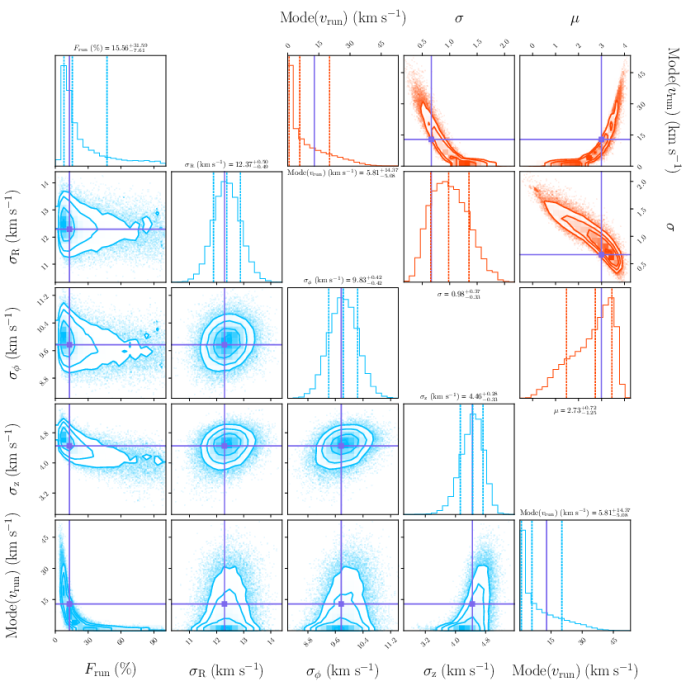
The runaway velocity distribution obtained through binary evolution in Sec. 3 has systematic errors due to gaps in our understanding of the physics of interacting, massive binary stars as well as the ad hoc definition of a Be star. This uncertainty can be quantified by loosening the requirement that the runaway velocity distribution is precisely the double log-normal obtained by our fit. Instead, we assume that the runaway velocity distribution is described by a log-normal distribution with two hyperparameters $\mu$ and $\sigma$. These hyperparameters have priors $\mu\sim\operatorname{Normal}(0,10)$ and $\sigma\sim\operatorname{Normal}(0.5,0.5)$. However, the data are sufficiently informative that the choice of these priors is not dominant. The posterior for this model is shown in the two corner plots of Fig. 14.

The mode of the posterior in $(\mu,\sigma)$ is close to the values which would replicate the single log-normal fit shown in Fig. 10. This implies that the runaway velocity distribution predicted in Sec. 3 is plausible. One of the key degeneracies in the posterior is between the runaway fraction and the mode of the runaway velocity distribution. A property of the log-normal distribution is that for $\mu<<\sigma^{2}$ the PDF can approximate a decay from the origin, i.e. all the probability is in runaway stars which have a zero runaway velocity, in which case all the Be stars can be runaway stars with no increase in their expected velocity. The existence of this degeneracy demonstrates that the total velocities of the Be stars are well constrained and that the model is simply changing the fraction of these velocities arising from either the velocity dispersion of the disc or the runaway velocity.

(a) Probability density functions.

(b) Cumulative density functions.

Figure 15: In grey, we show the 1, 2, and 3$\sigma$ contours of the log-normal distributions implied by the posterior of $(\mu,\sigma)$ shown in Fig. 14. The dark line is the log-normal given by the median of the posterior and the purple dashed line is the single log-normal fit to the simulated runaway velocity distribution shown in green in Fig. 10.

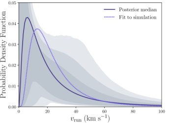
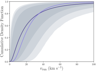
Each sampled point in the posterior corresponds to a different runaway velocity distribution. We take these velocity distributions and compute the 1, 2, and 3$\sigma$ contours of the probability and cumulative density functions at each value of $v_{\mathrm{run}}$, and compare in Fig. 15 to the single log-normal runaway velocity distribution shown in Fig. 10. The fit single log-normal is not an outlier in these plots which affirms that the runaway velocity distribution predicted by our simulations of binary stars is credible.

6 Discussion

We recall that, as shown in Sec. 3, a fraction of $17.5\%$ being runaways is consistent with all classical Be stars originating through mass transfer in binaries. This result arises because there is a substantial fraction of Be stars which remain bound post-supernova or avoid the supernova phase entirely. At $13.1\begin{subarray}{c}+2.6\\ -2.4\end{subarray}\%$, the posterior runaway fraction obtained in Section 5.3 is two standard deviations below this. We discuss below several possible explanations for this discrepancy.

6.1 Large uncertainty and wide velocity dispersion priors

Our weak prior on the global velocity dispersions may allow higher values to be taken at the expense of the number of runaways. Using the relations between age and velocity dispersions of Aumer & Binney (2009), we find that the posterior velocity dispersions imply that the population is around $200\;\mathrm{Myr}$ old, while the Be stars in our model population (accounting for selection effects) have a median age of $35.4\;\mathrm{Myr}$. It appears likely that the velocity dispersions are overestimated, with the caveat that it is likely that the Aumer & Binney (2009) velocity dispersions for young stars may be driven by their assumed functional form of the velocity dispersions with age,

$$\sigma(\tau)=v_{10}\left(\frac{\tau+\tau_{1}}{10\;\mathrm{Gyr}+\tau_{1}}\right)^{\beta}$$ (14)

where $v_{10}$ and $\tau_{1}$ characterize the velocity dispersion at $10\;\mathrm{Gyr}$ and at birth and $\beta$ describes the efficiency of stochastic acceleration. The degeneracy between the velocity dispersions and the number of runaways could be broken either by measuring the velocity dispersion of a population of runaway-free stars coeval to the Be stars or by exploiting the precise astrometry in Gaia DR2.

6.2 Uncertainty in binary stellar evolution

An alternative origin for the uncertainty is that the binary evolution simulations rely on a number of uncertain ingredients, some of which we discussed in Section 3.3 such as the natal kick distribution of compact objects, the fallback of material onto black holes and common envelope evolution. The use of different prescriptions for these aspects could easily resolve the discrepancy either by decreasing the frequency of runaway Be stars or shifting the runaway velocity distribution to smaller velocities (thus increasing the confusion between true runaways and fast disc stars).

More subtle changes to the binary evolution simulations could also account for part of the difference. For instance, if the prescription for tidal locking requires that the two stars need to be closer than is the case in reality, then the runaway velocity distribution of Be stars will be inflated to faster velocities. The details of the simulated population of Be stars are also sensitive to prescriptions describing mass transfer and rotation, both of which contain their own uncertainties.

Studies of single and binary stars using Gaia data over the next few years will drastically constrain these uncertainties in stellar evolution, which in turn will allow for a much keener inference to be made on the runaway fraction among Be stars.

6.3 Observational bias against runaway stars

Be stars are young and thus are typically found at low Galactic latitudes, because they do not live long enough for their vertical velocity to be excited through disc heating. However, runaway Be stars ejected out of the disc could have a large vertical velocity component and thus be found at high latitudes. There will be a trend in which high runaway velocity objects are more common at high latitudes. Considering the 40 high-likelihood runaway stars identified in Table 1, which are necessarily the fastest runaway stars in the catalogue, we see that all but two are within $400\;\mathrm{pc}$ of the Galactic plane. It is thus possible that our observational bias towards nearby objects may exclude some of the higher velocity Be runaway stars. If the discrepancy were to be entirely explained by this bias, we would need to miss the furthest 25% of Be stars from the disc.

To investigate this possibility, we sample 10,000 Be runaway stars with velocity dispersions given by the posterior in Section 5.3 and runaway velocities sampled from the model distribution obtained in Section 3.2. We assume the Be stars are born proportionally to the disc density found by Bovy & Rix (2013), noting that with a scale-height of $400\;\mathrm{pc}$ this is likely to over-estimate the number of high-latitude Be stars. The orbits of the sampled Be stars are then followed through the Milky Way using Galpy and the included MWPotential2014 potential (Bovy, 2015). Even with this vertically extended distribution of Be star birth locations, we find that only 20% of runaway Be stars should be found above $|z|=0.5\;\mathrm{kpc}$. Using a more realistic vertical dispersion of $100\;\mathrm{pc}$ derived from our observed sample of non-runaway stars, we find that only 3% of Be runaways should be found above $|z|=0.5\;\mathrm{kpc}$ and only 0.6% above $|z|=1.0\;\mathrm{kpc}$.

While this bias is not able to resolve the discrepancy, it does answer a long-standing open question which we discuss in the following subsection; Martin (2006) found that there were no Be stars among their 31 high-latitude ($|z|\gtrsim 1.0\;\mathrm{kpc}$) B runaway stars.

6.4 Should we find Be stars at high latitude?

Martin (2006) investigated the origin and evolutionary status of 48 B stars found far from the plane of the Milky Way and, surprisingly, found no Be stars in the sample despite the expectation of at least 10 Be stars based on the incidence of Be stars observed in the field by Zorec & Briot (1997). Previously, Slettebak et al. (1997) identified 8 Be stars between $0.2<\lvert z\rvert<0.9\;\mathrm{kpc}$ from the plane, which implies only a small overlap with the Martin (2006) sample covering $0.5<\lvert z\rvert<2.0\;\mathrm{kpc}$. Martin (2006) provides several arguments that could explain this absence:

1. The short baseline of the data may have missed temporarily inactive Be stars.

2. Magnitude-limited field studies are biased towards younger, brighter stars which have a higher rate of Be stars, i.e. the Be stars aren’t missing in this sample, merely overcounted in the field.

3. Based on the $v\sin i$ distribution and the lack of observed binaries among the dataset, the B stars may be mostly dynamically ejected from a cluster environment. It has been observed that there are fewer Be stars in clusters (although this may be a selection effect).

This list of solutions doesn’t consider the possibility that the Be phenomenon might be correlated with the runaway velocity, which could naturally explain the observations if very few Be stars are ejected at high enough velocities to reach high altitudes above the disc. This kinematic selection effect is mentioned by Martin (2006) who found that no star ejected with a velocity less than $50\;\mathrm{km}\;\mathrm{s}^{-1}$ can make it to $0.5\;\mathrm{kpc}$ above the disc even if the ejection velocity is aligned with the vertical. As we discussed in Section 6.3, only 3% of Be runaway stars should be found more than $0.5\;\mathrm{kpc}$ from the disc according to our predicted, selection-effect-included runaway velocity distribution, potentially contributing substantially to the solution of this problem.

7 Conclusions

In this work, we have shown that the first Gaia data release, specifically the Tycho-Gaia Astrometric Solution (TGAS), advances our understanding of the kinematics of Be stars. With future data releases of the full Gaia catalogue, we can expect to have a census of thousands of Be stars with precise kinematics.

We first constructed the largest catalogue of Be stars with full six-dimensional kinematics to date. This used three sources – namely, the Berger & Gies (2001) survey, the Be Star Spectra database (BeSS) and the catalogue of Hou et al. (2016) from LAMOST – crossmatching with TGAS where necessary to obtain updated proper motions and parallaxes. Our final combined catalogue contains 632 Be stars.

We then modelled the evolution of binaries across a grid in parameter space using the fast binary_c code (see e.g., Izzard et al., 2009) with a view to testing the post-mass-transfer model of Be stars (Pols et al., 1991). We computed the probability distribution for the runaway velocity and critical equatorial velocity ratio. We developed a criterion based on the equatorial velocity ratio for Be stars and thus obtained the distribution of runaway velocities and a prediction that 5% of all Be stars should be runaways (lower curve in Fig. 7(a)). We then demonstrated that it is vital to account for the observational bias towards early-type Be stars in our catalogue, because this changes our prediction for the population. For instance, we find that a fraction of $17.5\%$ Be stars in our catalogue being runaways is consistent with all classical Be stars originating through mass transfer in binaries, as the rest remain bound post-supernova or miss the supernova phase entirely.

To describe the kinematics of Be stars in our sample, we developed a Bayesian mixture model comprising three populations – thin disk stars, runaways and contaminants. The Bayesian model contained a total of 5067 parameters to represent the kinematics of 632 Be stars. Successfully tackling a Bayesian problem of this scope is a central achievement of this work. It allows us to go beyond fitting a runaway velocity distribution by modelling the distance, velocity dispersions and runaway fraction and velocities simultaneously. We verified that our method is both able to accurately retrieve the input parameters of an artificially-generated test set of stars and individually identify with low contamination the fastest third of the runaway stars. Applying to the true dataset, the posterior runaway fraction of Be stars is $13.1^{+2.6}_{-2.4}\%$. This suggests that some Be stars may originate through a process other than the post-mass-transfer scenario. However, caution is needed as there are a number of factors that may have caused us to underestimate the runaway fraction. In particular, there is a degeneracy between velocity dispersions of the thin disk stars and runaway fraction, and so a weak prior on the velocity dispersions may allow them to be overestimated at the cost of a low runaway fraction. The degeneracy between the velocity dispersions and number of runaway stars will be resolved by the precise astrometry in Gaia DR2. Additionally, there are a number of ingredients in binary stellar evolution (such as common envelope evolution and the distribution of compact object natal kicks) which are poorly understood and may be contributing to the discrepancy. We thus conclude that the predicted $17.5\%$ incidence of runaway stars among Be stars is consistent with our measured fraction and thus all Be stars could originate through the post-mass-transfer channel.

We also studied the expected distribution of Be stars at high Galactic latitude. We have argued that the dearth of Be stars in the high latitude runaway B star sample of Martin (2006) can be explained even if most of the runaways originate with the binary supernova scenario, because we would not expect runaway Be stars to have high enough velocities to reach high Galactic latitudes.

Although we have not fully resolved the contribution of the post-mass-transfer channel to the Be star population with the TGAS data, we are optimistic about the road ahead. The second and later Gaia data releases will increase the sample of Be stars with accurate kinematics by at least an order of magnitude; for instance, Hou et al. (2016) present a catalogue of 5187 Be stars in LAMOST, all of which will have proper-motions and parallaxes in Gaia DR2. The Bayesian approach developed in this work to tackle the kinematics of a large population lays the foundation for the full exploitation of this future dataset.

References

- Abate et al. (2013) Abate C., Pols O. R., Izzard R. G., Mohamed S. S., de Mink S. E., 2013, A&A, 552, A26
- Abate et al. (2015) Abate C., Pols O. R., Stancliffe R. J., Izzard R. G., Karakas A. I., Beers T. C., Lee Y. S., 2015, A&A, 581, A62
- Antoniou & Zezas (2016) Antoniou V., Zezas A., 2016, MNRAS, 459, 528
- Arzoumanian et al. (2002) Arzoumanian Z., Chernoff D. F., Cordes J. M., 2002, ApJ, 568, 289
- Astraatmadja & Bailer-Jones (2016) Astraatmadja T. L., Bailer-Jones C. A. L., 2016, ApJ, 832, 137
- Astropy Collaboration et al. (2013) Astropy Collaboration et al., 2013, A&A, 558, A33
- Aumer & Binney (2009) Aumer M., Binney J. J., 2009, MNRAS, 397, 1286
- Bailer-Jones (2015) Bailer-Jones C. A. L., 2015, PASP, 127, 994
- Berger & Gies (2001) Berger D. H., Gies D. R., 2001, ApJ, 555, 364
- Blaauw (1961) Blaauw A., 1961, Bulletin of the Astronomical Institutes of the Netherlands, 15, 265
- Boubert et al. (2017) Boubert D., Fraser M., Evans N. W., Green D. A., Izzard R. G., 2017, A&A, 606, A14
- Bovy (2015) Bovy J., 2015, ApJS, 216, 29
- Bovy & Rix (2013) Bovy J., Rix H.-W., 2013, ApJ, 779, 115
- Branch & Wheeler (2017) Branch D., Wheeler J. C., 2017, Supernova Explosions. Springer
- Carpenter et al. (2017) Carpenter B., et al., 2017, Journal of Statistical Software, 76
- Chernyakova et al. (2017) Chernyakova M., Babyk I., Malyshev D., Vovk I., Tsygankov S., Takahashi H., Fukazawa Y., 2017, MNRAS, 470, 1718
- Claeys et al. (2014) Claeys J. S. W., Pols O. R., Izzard R. G., Vink J., Verbunt F. W. M., 2014, A&A, 563, A83
- De Marco & Izzard (2017) De Marco O., Izzard R. G., 2017, PASA, 34, e001
- Duquennoy & Mayor (1991) Duquennoy A., Mayor M., 1991, A&A, 248, 485
- ESA (1997) ESA 1997, The Hipparcos and Tycho catalogues. Vol. 1200, ESA Special Publication, http://adsabs.harvard.edu/abs/1997ESASP1200.....E
- Eldridge et al. (2011) Eldridge J. J., Langer N., Tout C. A., 2011, MNRAS, 414, 3501
- Evans (1967) Evans D. S., 1967. p. 57, http://adsabs.harvard.edu/abs/1967IAUS...30...57E
- Faucher-Giguère & Kaspi (2006) Faucher-Giguère C.-A., Kaspi V. M., 2006, ApJ, 643, 332
- Foreman-Mackey (2016) Foreman-Mackey D., 2016, The Journal of Open Source Software, 2016
- Fryer et al. (2012) Fryer C. L., Belczynski K., Wiktorowicz G., Dominik M., Kalogera V., Holz D. E., 2012, ApJ, 749, 91
- Gaia Collaboration et al. (2016a) Gaia Collaboration et al., 2016a, A&A, 595, A1
- Gaia Collaboration et al. (2016b) Gaia Collaboration et al., 2016b, A&A, 595, A2
- Gelman & Rubin (1992) Gelman A., Rubin D. B., 1992, Statistical science, pp 457–472
- Gies et al. (1998) Gies D. R., Bagnuolo Jr. W. G., Ferrara E. C., Kaye A. B., Thaller M. L., Penny L. R., Peters G. J., 1998, ApJ, 493, 440
- Gontcharov (2006) Gontcharov G. A., 2006, Astronomy Letters, 32, 759
- González-Galán et al. (2018) González-Galán A., Oskinova L. M., Popov S. B., Haberl F., Kühnel M., Gallagher J., Schurch M. P. E., Guerrero M. A., 2018, MNRAS, 475, 2809
- Hansen & Phinney (1997) Hansen B. M. S., Phinney E. S., 1997, MNRAS, 291, 569
- Hansen et al. (2004) Hansen C. J., Kawaler S. D., Trimble V., 2004, Stellar Interiors: Physical Principles, Structure, and Evolution, 2 edn. Astronomy and Astrophysics Library, Springer-Verlag, New York, //www.springer.com/gb/book/9780387200897
- Harmanec (1987) Harmanec P., 1987. IAU Colloq. 92: Physics of Be Stars, pp 339–355, http://adsabs.harvard.edu/abs/1987pbes.coll..339H
- Harmanec et al. (1972) Harmanec P., Koubský P., Krpata J., 1972, Astrophysical Letters, 11, 119
- Hartman (1997) Hartman J. W., 1997, A&A, 322, 127
- Hobbs et al. (2005) Hobbs G., Lorimer D. R., Lyne A. G., Kramer M., 2005, MNRAS, 360, 974
- Hoffman & Gelman (2011) Hoffman M. D., Gelman A., 2011, preprint, 1111, arXiv:1111.4246
- Hoogerwerf et al. (2001) Hoogerwerf R., de Bruijne J. H. J., de Zeeuw P. T., 2001, A&A, 365, 49
- Hou et al. (2016) Hou W., et al., 2016, Research in Astronomy and Astrophysics, 16, 138
- Hunter (2007) Hunter J. D., 2007, Computing In Science & Engineering, 9, 90
- Hurley et al. (2000) Hurley J. R., Pols O. R., Tout C. A., 2000, MNRAS, 315, 543
- Hurley et al. (2002) Hurley J. R., Tout C. A., Pols O. R., 2002, MNRAS, 329, 897
- Høg et al. (2000) Høg E., et al., 2000, A&A, 355, L27
- Izzard et al. (2004) Izzard R. G., Tout C. A., Karakas A. I., Pols O. R., 2004, MNRAS, 350, 407
- Izzard et al. (2006) Izzard R. G., Dray L. M., Karakas A. I., Lugaro M., Tout C. A., 2006, A&A, 460, 565
- Izzard et al. (2009) Izzard R. G., Glebbeek E., Stancliffe R. J., Pols O. R., 2009, A&A, 508, 1359
- Izzard et al. (2018) Izzard R. G., Preece H., Jofre P., Halabi G. M., Masseron T., Tout C. A., 2018, MNRAS, 473, 2984
- Jaschek et al. (1981) Jaschek M., Slettebak A., Jaschek C., 1981, Be Star Newsletter, 4, 9
- Jing et al. (2016) Jing Y., et al., 2016, MNRAS, 463, 3390
- Johnson & Soderblom (1987) Johnson D. R. H., Soderblom D. R., 1987, ApJ, 93, 864
- Jones et al. (2001) Jones E., Oliphant T., Peterson P., others 2001, SciPy: Open source scientific tools for Python. http://www.scipy.org/
- Kharchenko et al. (2007) Kharchenko N. V., et al., 2007, Astronomische Nachrichten, Astronomische Nachrichten, 328, 328, 889, 889
- Kroupa (2001) Kroupa P., 2001, MNRAS, 322, 231
- Liu et al. (2015) Liu Z.-W., Tauris T. M., Röpke F. K., Moriya T. J., Kruckow M., Stancliffe R. J., Izzard R. G., 2015, A&A, 584, A11
- Martin (2006) Martin J. C., 2006, AJ, 131, 3047
- McKinney (2010) McKinney W., 2010, in Walt S. v. d., Millman J., eds, Proceedings of the 9th Python in Science Conference. pp 51 – 56
- Nazé et al. (2017) Nazé Y., Rauw G., Cazorla C., 2017, A&A, 602, L5
- Neiner et al. (2011) Neiner C., de Batz B., Cochard F., Floquet M., Mekkas A., Desnoux V., 2011, AJ, 142, 149
- Nelemans et al. (1999) Nelemans G., Tauris T. M., van den Heuvel E. P. J., 1999, A&A, 352, L87
- Perets (2009) Perets H. B., 2009, ApJ, 698, 1330
- Peters et al. (2008) Peters G. J., Gies D. R., Grundstrom E. D., McSwain M. V., 2008, ApJ, 686, 1280
- Peters et al. (2013) Peters G. J., Pewett T. D., Gies D. R., Touhami Y. N., Grundstrom E. D., 2013, ApJ, 765, 2
- Peters et al. (2016) Peters G. J., Wang L., Gies D. R., Grundstrom E. D., 2016, ApJ, 828, 47
- Pflamm-Altenburg & Kroupa (2010) Pflamm-Altenburg J., Kroupa P., 2010, MNRAS, 404, 1564
- Pols et al. (1991) Pols O. R., Cote J., Waters L. B. F. M., Heise J., 1991, A&A, 241, 419
- Popper (1988) Popper D. M., 1988, AJ, 95, 1242
- Poveda et al. (1967) Poveda A., Ruiz J., Allen C., 1967, Boletin de los Observatorios Tonantzintla y Tacubaya, 4, 86
- Reed (2003) Reed B. C., 2003, AJ, 125, 125, 2531, 2531
- Reig (2011) Reig P., 2011, Astrophysics and Space Science, 332, 1
- Rinehart (2000) Rinehart S. A., 2000, MNRAS, 312, 429
- Rivinius et al. (2006) Rivinius T., Štefl S., Baade D., 2006, A&A, 459, 137
- Rivinius et al. (2013) Rivinius T., Carciofi A. C., Martayan C., 2013, Astronomy and Astrophysics Review, 21, 69
- Sana et al. (2012) Sana H., et al., 2012, Science, 337, 444
- Schneider et al. (2014) Schneider F. R. N., et al., 2014, ApJ, 780, 117
- Schönrich (2012) Schönrich R., 2012, MNRAS, 427, 274
- Schönrich et al. (2010) Schönrich R., Binney J., Dehnen W., 2010, MNRAS, 403, 1829
- Scott (2015) Scott D. W., 2015, Multivariate density estimation: theory, practice, and visualization. John Wiley & Sons
- Slettebak et al. (1997) Slettebak A., Wagner R. M., Bertram R., 1997, PASP, 109, 1
- Spera et al. (2015) Spera M., Mapelli M., Bressan A., 2015, MNRAS, 451, 4086
- Struve (1931) Struve O., 1931, ApJ, 73, 94
- Tauris & Takens (1998) Tauris T. M., Takens R. J., 1998, A&A, 330, 1047
- Townsend et al. (2004) Townsend R. H. D., Owocki S. P., Howarth I. D., 2004, MNRAS, 350, 189
- Walt et al. (2011) Walt S. v. d., Colbert S. C., Varoquaux G., 2011, Computing in Science Engineering, 13, 22
- Wang et al. (2017) Wang L., Gies D. R., Peters G. J., 2017, ApJ, 843, 60
- Wenger et al. (2000) Wenger M., et al., 2000, A&AS, 143, 9
- Wilson (1953) Wilson R. E., 1953, Carnegie Institute Washington D.C. Publication
- Zapartas et al. (2017) Zapartas E., et al., 2017, A&A, 601, A29
- Zorec & Briot (1997) Zorec J., Briot D., 1997, A&A, 318, 443
- de Mink et al. (2013) de Mink S. E., Langer N., Izzard R. G., Sana H., de Koter A., 2013, ApJ, 764, 166
- van Rensbergen et al. (1996) van Rensbergen W., Vanbeveren D., De Loore C., 1996, A&A, 305, 825
- van den Heuvel et al. (2000) van den Heuvel E. P. J., Portegies Zwart S. F., Bhattacharya D., Kaper L., 2000, A&A, 364, 563