TIFR/TH/18-9
Pinning down Anomalous Couplings at the LHC
Disha Bhatia1, Ushoshi Maitra2 and Sreerup Raychaudhuri3
Department of Theoretical Physics, Tata Institute of Fundamental
Research,
1 Homi Bhabha Road, Mumbai 400 005, India.
Abstract
We make a careful analysis of production at the LHC, identifying the through leptonic decays, with a view to exploring the sensitivity of the machine to anomalous -conserving interactions. All the available kinematic variables are used, but we find that the most useful one is the opening angle in the transverse plane between the decay products of the . It is shown that even a simple-minded analysis using this variable can lead to a much greater sensitivity at the LHC than the current constraints on the relevant parameters.
The initial euphoria over the Higgs boson discovery of 2012[1] has now more-or-less abated, and even after more than a year’s running of the CERN Large Hadron Collider (LHC) at the upgraded energy of 13 TeV, there have been no signs of new physics beyond the Standard Model (SM)[2]. However, while it has become abundantly clear that the belief that new particles and interactions would be discovered as soon as the LHC upgrade began to run was overly optimistic, there is no reason for despondency — as yet[3]. This is because most of the new physics models proposed are of the decoupling type, with (possibly) highly massive particles and very feeble interactions, and may therefore prove much more difficult to discover than we have hitherto imagined – or hoped. At this juncture, we may quickly fortify ourselves by noting that the last serendipitous discovery of an elementary particle (the -lepton) occurred more than forty years ago, and that both the Higgs boson and the phenomena of neutrino oscillations took about the same time or even longer to establish experimentally. It is probably necessary, therefore, for high energy physicists to settle down for a long, hard grind before the expected new physics effects can be observed. For exist they must, if our ideas about quantum field theory, gravitation and cosmology are at all correct[4]. In any case, that a theory with as many ad hoc features as the SM can be the ultimate truth about Nature is unacceptable to many.
If we assume that there is new physics, but it consists of particles too massive to be discovered at the LHC, at least in the early stages of its 13 TeV run, then the only way in which these particles can be observed is through quantum effects, either at the tree or the loop levels. These will appear as modifications to the SM vertices, or the appearance of new, often higher-dimensional, operators involving the SM fields, with coefficients which are rendered small by the heavy mass scale of the underlying physics. Such effective field theories – involving only the field content of the SM – seem to offer the most promising window into physics beyond the SM[5]. However, effective theories have their own problem. Most so-called UV-complete models beyond the Standard Model have only a limited set of operators because of the twin constraints of gauge invariance (or extended gauge symmetries)
E-mail: 1disha@theory.tifr.res.in
2ushoshimaitra32@gmail.com
3sreerup@theory.tifr.res.in
and renormalisability. In contrast, effective field theories may have a low-lying cutoff, which removes the requirement of renormalisability and permits a proliferation of operators – all with small, but unknown coefficients. With so many unknown parameters, and only a finite set of measurables, almost any phenomenon can, in general, be explained and almost any prediction can be made. This is, if anything, a worse situation than the minimal SM even with all its ad hoc features.
It follows from the above that the broad picture of effective field theories is not perhaps the best approach to probe of physics beyond the SM. The focus in recent times has been, therefore, on a more minute examination of the operators, and on measurables which depend significantly on only a limited set of these operators, rather than the whole set – an exercise which goes under the misnomer of simplified models, for it is the examination rather than the model which is simplified. Perhaps one of the earliest of these focussed examinations has been that of anomalous triple gauge-boson couplings (TGCs) [6, 7], which started from the days of the LEP collider[8] and have acquired new relevance in the present climate[9, 10, 11]. These are anomalous, of course, only in the sense of being absent in the SM at tree level. The TGC’s which have been considered are possible modifications to the and vertices, and possible new , and vertices [12].
![[Uncaptioned image]](/html/1804.05357/assets/x1.png)
This article takes just one of these vertices, viz, the vertex illustrated on the left and considers a specific final state which is affected by only changes to this vertex. The process in question is
where the for and perhaps .
If we denote the vertex by , then the most general -conserving form consistent with the gauge and Lorentz symmetries of the SM can be parametrised[6] in the form of three separate terms, viz.
| (1) |
where the tensors are, respectively,
| (2) | |||||
The tensor in Eq. (S0.Ex4) corresponds to the Standard Model coupling, while the tensors and give rise to anomalous TGC’s. It may be noted that the dimension-4 tensor can be absorbed in with a coefficient . However, in our work we have kept these tensors distinct as representing the SM and beyond-SM parts. Thus and parametrise the strength of these beyond-SM contributions — which agrees with the common usage by most experimental collaborations111Strictly speaking, there are SM contributions to and at higher orders. For example, at the one-loop level, there could be contributions of the order of (few) at a centre-of-mass energy of TeV strength[13]. These are negligible in the current experimental studies, which, till date, only put constraints at the level of .. It is reasonable to assume that will not be more than a few percent, for otherwise these corrections would have been detected when the itself was discovered, or when its properties were precisely measured at the CERN LEP-2[15] and the Fermilab Tevatron[16]. It is also traditional to parametrise the mass-suppression of the dimension-6 operator with a factor . However, if the operator arises from new physics at a scale , the corresponding coefficient should have been , where is some coupling – perhaps – and hence, we can identify
| (3) |
In fact, setting , and TeV, we get . We may thus expect to lie an order of magnitude below , and, in fact, we shall see below that this is indeed true for the experimental constraints.
We remark in passing that there are also -violating contributions to the vertex, which can be parametrised in terms of two coupling constants and . However, these are already constrained to be very small from the measurement of the electric dipole moment of the neutron[17], and hence we will not consider them further in this article. It is also possible – in fact, plausible – that if the photon has anomalous couplings with a pair, then the boson may also have such anomalous couplings, which may be related in some way by the gauge invariance of the SM[6]. However, the philosophy adopted in this article is that these will not affect the measurement in question, and can therefore, be kept outside the scope of the discussion. Experimental bounds involving production [15, 18, 19] have to consider this possibility and hence always carry a caveat about the choice of couplings.
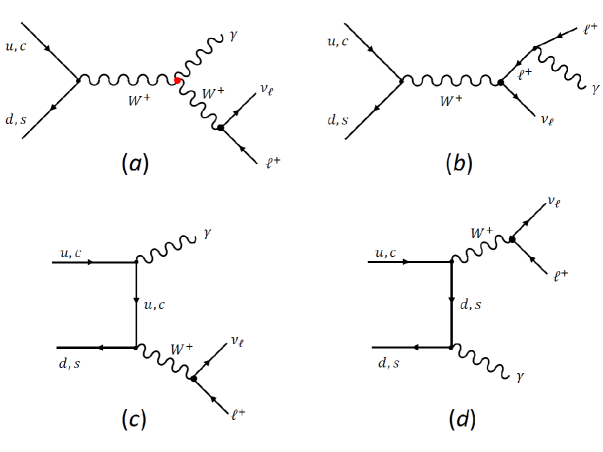
The production of a associated with a hard transverse photon is one of the most standard processes which one considers at a hadron collider[21, 20]. It occurs through a pair of dissimilar quarks, e.g. and , as the initial-state partons, which are required for single boson production. A photon can then be radiated off any of the internal or external legs of the corresponding diagram. However, if we allow the to decay further into a charged lepton and the corresponding neutrino , we will have one more diagram where a photon is radiated off the charged lepton. The final state consists, then, of a photon, a lepton and missing energy from the neutrino. One would also require a jet veto to keep the process hadronically quiet. The four diagrams at leading order are illustrated in Fig. 1.
When these diagrams are evaluated, the Feynman amplitude can be written
| (4) |
squaring which, it follows that the cross-section will be a combination of terms
| (5) | |||||
where the terms on the first line of Eq. (5) arise from the squares of the corresponding terms in Eq. (4), while the terms on the second line are the respective interference terms. Since and are small, it is clear that will be the dominant term – or dominant background – while the other terms in Eq. (5) will constitute a small signal. Of these, the terms linear in and will generally be the largest. The challenge is, therefore, to isolate the extremely small signal from the large SM background by the judicious use of kinematic cuts and distributions. At this point, we note that QCD corrections to the process may increase[22] the overall cross-section by %. However, these may be expected to be rather similar for both signal and background, and hence are not taken into account in our analysis.
In the experimental situation, our concern is with a hadronically-quiet final state consisting of a hard transverse photon, a hard transverse lepton and substantial missing energy. This is a very clean signal and, barring issues like pileup and multiple interactions at the LHC, may be expected to constitute a strong probe for the underlying physics – in this case, the TGC concerned. Since the final state is so simple, there exists only a small number of kinematic variables which are invariant under longitudinal boosts, and these, together with the cuts we have imposed on them, are listed below.
-
(A)
The magnitude of the transverse momentum of the photon (), which we require to satisfy GeV.
-
(B)
The pseudorapidity of the photon (), which we require to satisfy .
-
(C)
The magnitude of the transverse momentum of the lepton (), which we require to satisfy GeV.
-
(D)
The pseudorapidity of the lepton (), which we require to satisfy .
-
(E)
The magnitude of the missing transverse momentum (), which we require to satisfy GeV.
-
(F)
The so-called angular separation between photon and lepton (), which we require to satisfy .
The cuts in (A) – (E) are driven more by ease of identification of the final state and the detector coverage, while (F) is included to suppress the collinear photons which are preferred by the SM diagrams in Fig 1(b)-(d).
In addition to the above, if we consider the vector momenta in the transverse plane, which we denote , and , we can construct three more variables which are invariant under longitudinal boosts. These are
| (6) |
These angular variables are known to be highly sensitive to momentum-dependent operators[9] and since the tensors are of this kind, we may expect them to carry some signs of the anomalous TGCs. In fact, we find that the only variables which are sensitive to these are the transverse momenta in (A), (C) and (E) above, and these angular variables in Eq. (6).
| Cut | |||
|---|---|---|---|
| GeV | 430.11 fb | 737.82 fb | 41.89 pb |
| GeV | 100.0 % | 100.0 % | 100.0 % |
| GeV | 70.25 % | 75.70 % | 85.55 % |
| GeV | 22.82 % | 52.34 % | 70.77 % |
| GeV | 20.68 % | 43.13 % | 55.11 % |
| 15.89 % | 36.88 % | 53.50 % | |
| 12.28 % | 32.61 % | 52.24 % | |
| 11.30 % | 32.60 % | 52.26 % | |
| 48.57 fb | 240.52 fb | 21.89 pb |
Finally, to ensure good convergence of our Monte Carlo simulations, we construct[20, 21] the variable , where
| (7) |
and impose a cut GeV. The effect of these successive kinematic cuts on the terms in the cross-section is shown in Table 1. Any stronger cuts would result in severe loss in the TGC signal, both for and .
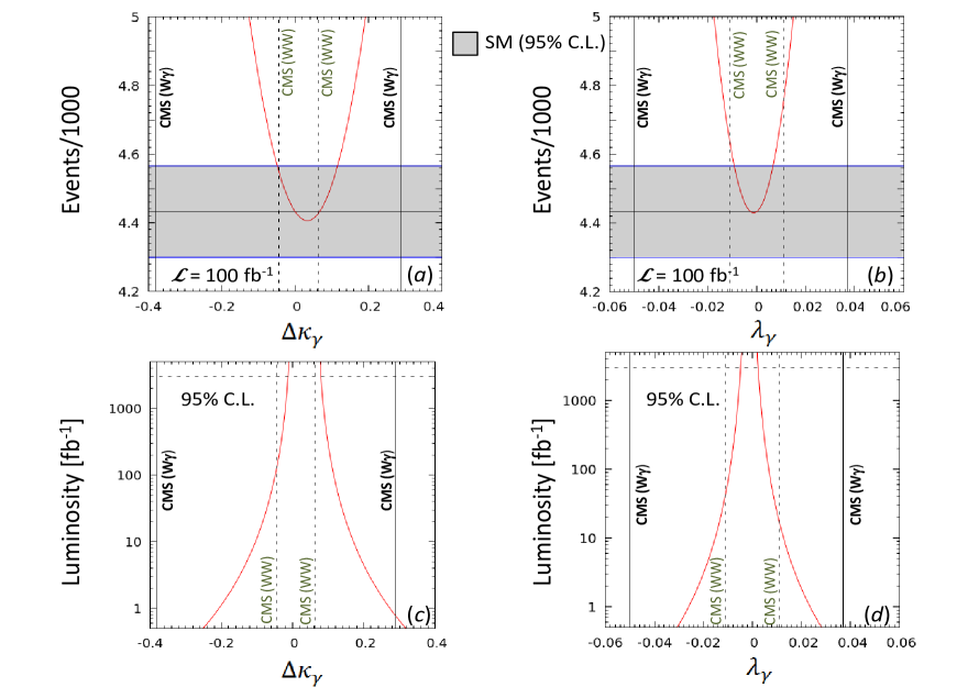
If we consider the total cross-section, as given above, the limits one can put on the parameters and are already strong. The actual number of signal events (in thousands) expected are shown in the panels marked () and () in Fig. 2, assuming an integrated luminosity of 100 fb-1. The abscissa in () and () shows, respectively, the values of and , each assuming that the other is zero. The region marked in grey corresponds to the 95% confidence level (C.L.) fluctuation in the SM prediction. Solid vertical lines indicate the current experimental bounds from production at the LHC[21, 20], which directly constrains the vertex, whereas broken vertical lines indicate the bounds from production[18, 19], where there are contributions from both and vertices. As explained above, these constraints are not as solid as those obtained from production. However, it is immediately obvious that the signal considered in this work can achieve the 95% C.L. level even at values which are comparable with the constraints, and certainly far smaller than the current constraints.
If the plots in the upper panels of Figure 2 indicate strong constraints with a luminosity of 100 fb-1, it is relevant to ask what may be achieved at the high-luminosity upgrade of the LHC (HL-LHC), where the integrated luminosity may go as high as 3 ab-1. To determine the search limits, we can determine the signal significance as a function of luminosity as
| (8) |
assuming Gaussian random fluctuations in the background . For this study, we ignore systematic errors, or, more properly, assume that they will be small enough to be ignored, compared to the statistical error. Now if, for a given value of , the value(s) of and/or satisfies , we qualify the signal for an anomalous TGC as observable at 95% C.L. The corresponding variations, for the cases (c) and (d) are plotted in the lower panels of Figure 2. It may immediately be seen that even with a very low integrated luminosity, the 13 TeV LHC does immensely better than the Run-1 data, and with an integrated luminosity of 1 ab-1, the direct constraints from the total cross-section are better than those even from production (which involve the couplings), except for one case . At this juncture it is relevant to note the asymmetry of the curves in each panel about the zero point, which can be attributed to large interference terms between the anomalous operators and the SM ones.
We now address the principal question for which this work was taken up, and that is whether the study of differential cross-sections instead of the total cross-section can help better in identifying anomalous couplings. We have made a careful study of practically all the straightforward kinematic variables it is possible to construct with a final state. It turns out that the ones which are sensitive to the anomalous couplings, i.e. the ones for which the anomalous operators behave differently than the SM operators, are those listed below:
| () | () | () | () | () | () | |
|---|---|---|---|---|---|---|
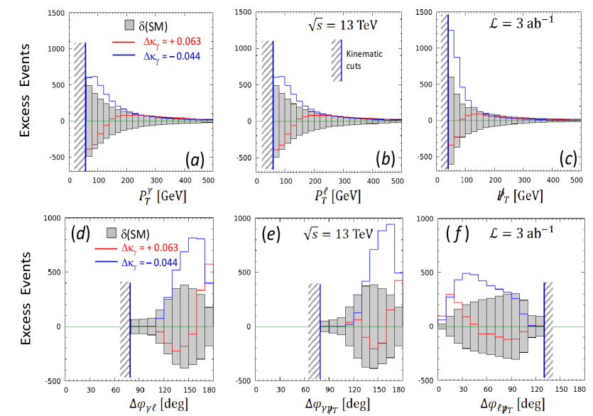
The effect of the anomalous TGCs on these is, of course, different for different observables, and this is illustrated in Figures 3 and 4. In Figure 3 we show three histograms in each panel, for the bin-wise quantity
| (9) |
where is the integrated luminosity and is the corresponding variable in Table 2. In each panel of Figure 3, the red histogram corresponds to the excess events as per Eqn. (9) for , i.e. the more stringent CMS upper limit arising from the cross-section[19], and the blue histogram indicates the corresponding lower limit . The solid shaded region represents the 95% C.L. fluctuations in the SM prediction, denoted . In each case, the kinematic cuts listed in the text above are shown by a vertical line and hatching. For these plots, we have set ab-1, i.e., the maximum envisaged value of the HL-LHC.
If we consider the case of , i.e. the red histograms in Figure 3, we can see that the number of excess events is substantially above the SM fluctuation for a significant number of bins, especially as one goes towards higher magnitudes of and for back-to-back vectors in the transverse plane, except for the opening angle in the transverse plane between the decay products of the , which tend to be aligned for the signal. In fact, in some of the bins, the deviation is rather large. One the other hand, if we consider the case of , i.e. the blue histograms in Figure 3, the deviations are large only for really high magnitudes of and even more extreme angles in the transverse plane than in the case of positive .
Some of the salient features of the histograms in Figure 3 are listed below.
-
•
In all the panels, the signal histograms for negative change sign over the selected range, whereas for positive they are monotone.
-
•
Of the upper three panels, clearly the best signal will come from a study of the missing , for, even for negative , there are significant deviations over 100 GeV.
-
•
In the lower three panels, all show large deviations from the SM background. It is not clear by inspection which of these three variables is best suited to find the signal. For this, we must develop a suitable numerical metric.
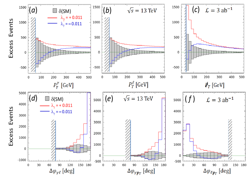
We then turn to the other anomalous coupling , in the case when . This is illustrated in Figure 4, where we show the same three histograms in each panel as for Figure 3, for the bin-wise quantities as defined in Eqn. (9) and the table below it. The notations and conventions of Figure 4 are therefore identical with those of Figure 3. Obviously the range of values of is smaller, but this is, as explained before, due to the artificial scaling with instead of some higher scale. Thus, the red (blue) histograms correspond to , which are, as before, the CMS limits from production[19]. Qualitatively, the deviations are rather similar to those in Figure 3, and one cannot tell, just by inspection, which of the parameters is preferable. Thus, if indeed, a deviation in these distributions from the SM prediction is found, we will encounter a difficult inverse problem, i.e. separation of signals from from those for . In the present article, however, we feel that it is premature to address this problem. Instead, we focus on whether it will be possible to extend the discovery reach of the LHC by considering these distributions, rather than the total cross-section. The time to address this distinction will come when a deviation is actually found.
In order to see if a distribution has enough deviation from the SM prediction to be observable at, say, 95% C.L., we need to construct a suitable numerical metric. We choose a simple-minded extension of the one in Eqn. (8), in the form
| (10) |
where the index runs over all the bins, and
| (11) |
is the SM prediction in that bin. is defined in Eqn. (9), but here it carries a bin index , and is, as usual, the integrated luminosity. The total number of bins is not the same for all the different variables , as a glance at Figures 3 and 4 will show. We can now compare the calculated values of with which is the probability that the SM cross-section with bins will undergo a 95% Gaussian fluctuation, faking a signal. If, for a given set of arguments, , we will assume the corresponding anomalous TGC to be discoverable at the LHC.
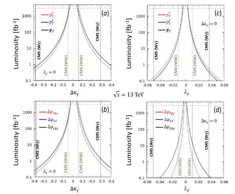
Our results for the different variables are shown in Figure 5. The upper panels, marked () and () show the discovery limits for the transverse momentum variables , and in the two cases () and () respectively. Corresponding limits for the azimuthal angle variables , and are similarly shown in the lower panels, marked () and () respectively. As before, the CMS limits from production[21], as well as those from production[19] are shown by solid and broken vertical lines respectively. As in Figure 2, a broken horizontal line represents the maximum integrated luminosity envisaged at the HL-LHC, and therefore, its intersections with the different curves indicates the discovery limit of the machine.
If we now inspect the discovery limits in Figure 5 and compare then with those in Figure 2, the following conclusions emerge.
-
•
For , the discovery limits from the total cross-section are better than those from the distributions; among the distributions, the best constraints arise from .
-
•
For , the discovery limits from the total cross-section are no longer better; instead the distributions are more efficient, especially as the luminosity increases above 100 fb-1. The distribution can be used to get discovery limits comparable to those from the different distributions, but not better.
-
•
For , the total cross-section and the distributions give similar discovery limits, while the discovery limits from the are significantly better and obviously improve as the integrated luminosity increases.
-
•
For , the total cross-section gives better discovery limits than the distributions, whereas the distribution always gives better sensitivity.
It is also interesting to note that of the three distributions, the best results are obtained from different distributions in different regimes, whereas for the distributions, is always the most sensitive. This sensitivity is likely to be due to interference between different helicity amplitudes [14], though that is not explicit in our calculations.
There is a very important lesson to learn from the above observations, viz., that there is no unique variable whose study will provide the maximum sensitivity to anomalous TGCs. A proper experimental study should, therefore, include all the variables considered above, including the total cross-section. Currently, experimental results are mostly based on transverse momentum studies[15, 20, 21], but these, as our results indicate, are not always the most sensitive variables.
Thus far, we have only considered one of the TGCs at a time, viz., either , or . While convenient from a purely phenomenological standpoint, this is hard to justify from a top-down approach, for the same new physics which creates nonzero could very well generate nonzero as well. We now turn, therefore, to the study of this more realistic case of joint variation of the two parameters. The formulae in Eqns. (8) and (10) are naturally geared to handle this joint variation, so all that is required is to numerically vary both the parameters and perform the same kind of analysis as we have described above.
Our results for joint variation are shown in Figure 6. The left panel, marked () shows the discovery limits that can be obtained using the total cross-section. The inaccessible region at the 13 TeV LHC, assuming an integrated luminosity of 10(1000) fb-1 is shaded in pink(red). For comparison, on the same panel we give the constraints from LEP-2 (black), and from the CMS (blue) and ATLAS (green) Collaborations at the LHC Run-1. In each case the inside of the ellipse is not accessible and the region outside is ruled out. It is immediately obvious that, as was the case with one parameter at a time, the total cross-section is a reasonably sensitive probe of anomalous TGCs, and in fact, even with 10 fb-1 of data, it is as sensitive as the use of the production data (modulo the caveat). Sensitivity improves dramatically for 1000 fb-1 luminosity, as the tiny red shaded region indicates. However – and here lies the rub – the inaccessible region is star-shaped, with four arms which stretch to possible large values of one of the parameters at a time. It is easy to see why these arise, for the significance is based on a single parameter, viz., the total cross-section, and there will always be regions where the contributions to this from cancel with those from , making the signal small or vanishing. Thus, although the total cross-section can be used to probe the anomalous TGCs quite efficiently, there remain these four narrow wedges of the parameter space which are inaccessible to the LHC.
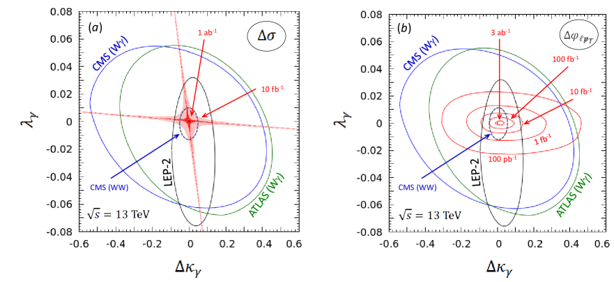
The situation can be radically improved by using a distribution, rather than the total cross-section, for it is almost inconceivable that the extra contributions from will undergo a bin-by-bin cancellation with those from , given that the distributions are somewhat different, as shown in Figures 3 and 4. To be precise, the same pair of values which cause cancellation of anomalous effects in one bin, may not cause cancellation in another bin, and hence, the overall value of will not be rendered small. This is illustrated in the right panel, marked () of Figure 6, where we use the distribution in to obtain 95% C.L. discovery limits. Here, corresponding to different values of the integrated luminosity, we show the discovery limits as elliptic regions in the same way as shown by the experimental collaborations. As usual, the interior of each ellipse is inaccessible to the LHC with the luminosity in question. The experimental constraints are given exactly as in the left panel, marked (). It hardly needs to be commented that at the HL-LHC, very stringent constraints indeed could be obtained in case no deviation from the SM is seen. It may be noted, however, that even with this accuracy of measurement, the one-loop SM effects will not be accessible, though effects from new physics such as the MSSM, may be[13] .
To summarise, then, we have considered the process at the 13 TeV run of the LHC, and studied possible implications of having anomalous (-conserving) vertices in the theory. The choice of this process (which has a lower cross-section than, say, pair production) is because the tagging of a final-state photon ensures that there is no contamination of the new physics contribution with possible anomalous effects in the vertex. We have shown that the anomalous couplings may be constrained by considering not one, but seven independent observables, viz. the total cross-section, three different distributions and three different azimuthal angle variables. The relative efficacy of each of these has been studied in detail, making certain simplifying assumptions, such as the absence of initial/final state radiation, pileup effects, systematic errors and detector effects. The first two we expect to be essentially eliminated by the rather severe kinematics cuts chosen for our analysis, but the latter ones can only be estimated by a thorough experimental analysis, which is beyond the scope of this work. Similarly, we have assumed that the kinematic cuts suggested by us will be effective in controlling backgrounds from + jet events (with a jet faking a photon). Under these assumptions, we have shown that the judicious use of the variables studied, especially the azimuthal angle variable , can be used to pinpoint anomalous effects in the process in question, to a great degree of accuracy, as the statistics collected by the LHC (and its HL upgrade) grow larger. Such measurements would eventually probe not just large electoweak corrections in the TGC sector, but could also effectively constrain new physics involving modifications and mixings in the gauge sector. Of course, the most exciting scenario would be to see an unambiguous deviation from the SM prediction in any of the variables (or more than one variable) in the upcoming runs of the LHC, and it is on this hopeful note that we conclude this article.
Acknowledgements: The authors are grateful to Sandhya Jain and Gobinda Majumder (CMS Collaboration) for discussions.
References
-
[1]
G. Aad et al. [ATLAS Collaboration],
Phys. Lett. B 716, 1 (2012) ;
S. Chatrchyan et al. [CMS Collaboration], Phys. Lett. B 716, 30 (2012). -
[2]
ATLAS Collaboration, Summary Plot for SUSY,
https://atlas.web.cern.ch/Atlas/GROUPS/PHYSICS/CombinedSummaryPlots/ SUSY/ATLAS_SUSY_Summary/
ATLAS_SUSY_Summary.png ;
ATLAS Collaboration, Summary Plot for Exotics,
https://atlas.web.cern.ch/Atlas/GROUPS/PHYSICS/CombinedSummaryPlots/EXOTICS/ATLAS_Exotics_Summary/
ATLAS_Exotics_Summary.png ;
CMS Combined Summary Plot,
https://twiki.cern.ch/twiki/pub/CMSPublic/PhysicsResultsCombined/exo-limits_ICHEP_2016.001.png. - [3] J. Hewett, Theory Summary, delivered at the 53rd Recontres de Moriond (La Thuile, Italy), March 2018.
- [4] See, for example, J. Ellis, Phil. Trans. Roy. Soc. Lond. A 370, 818 (2012).
-
[5]
W. Büchmuller and D. Wyler, Nucl. Phys. B 268, 621 (1986).
For a more recent review, see S. Dawson, TASI 2016 Lectures, arXiv:1712.07232 [hep-ph]. - [6] K. Hagiwara, R. D. Peccei, D. Zeppenfeld and K. Hikasa, Nucl. Phys. B 282, 253 (1987).
- [7] K. Hagiwara, S. Ishihara, R. Szalapski and D. Zeppenfeld, Phys. Lett. B 283, 353 (1992).
- [8] U. Baur and D. Zeppenfeld, Phys. Lett. B 201, 383 (1988).
-
[9]
S. S. Biswal, R. M. Godbole, B. Mellado and S. Raychaudhuri,
Phys. Rev. Lett. 109, 261801 (2012) ;
S. S. Biswal, M. Patra and S. Raychaudhuri, arXiv:1405.6056 [hep-ph] ;
A. Azatov, J. Elias-Miro, Y. Reyimuaji and E. Venturini, JHEP 1710, 027 (2017) ;
R. Li, X. M. Shen, K. Wang, T. Xu, L. Zhang and G. Zhu, arXiv:1711.05607 [hep-ph]. -
[10]
G. Buchalla, O. Cata, R. Rahn and M. Schlaffer, Eur. Phys. J. C 73,
2589 (2013) ;
L. Bian, J. Shu and Y. Zhang, JHEP 1509, 206 (2015) ;
A. Rosca, Nucl. Part. Phys. Proc. 273-275, 2226 (2016) ;
J. D. Wells and Z. Zhang, Phys. Rev. D 93, 034001 (2016) ;
S. M. Etesami, S. Khatibi and M. Mohammadi Najafabadi, Eur. Phys. J. C 76, 533 (2016) ;
R. Rahaman and R. K. Singh, arXiv:1711.04551 [hep-ph] ;
A. Falkowski et al., JHEP 1702, 115 (2017) ;
Z. Zhang, Phys. Rev. Lett. 118, 011803 (2017). -
[11]
T. Corbett et al.,
Phys. Rev. Lett. 111, 011801 (2013) ;
A. Butter, et al, JHEP 1607, 152 (2016). - [12] D. R. Green, P. Meade and M. A. Pleier, Rev. Mod. Phys. 89, 035008 (2017).
- [13] G. Gounaris et al., hep-ph/9601233.
- [14] G. Panico, F. Riva and A. Wulzer, Phys. Lett. B 776, 473 (2018).
- [15] See, for example, S. Schael et al. [ALEPH, DELPHI, L3 and OPAL, LEP Electroweak Collaborations], Phys. Rept. 532, 119 (2013).
- [16] See, for example, C. E. Gerber et al. [TeV4LHC-Top Collaboration and Electroweak Working Group], arXiv:0705.3251 [hep-ph].
-
[17]
F. Boudjema, K. Hagiwara, C. Hamzaoui and K. Numata,
Phys. Rev. D 43, 2223 (1991) ;
D. Choudhury, J. Kalinowski and A. Kulesza, Phys. Lett. B 457, 193 (1999). - [18] M. Aaboud et al. [ATLAS Collaboration], Eur. Phys. J. C 77, 563 (2017).
- [19] A. M. Sirunyan et al. [CMS Collaboration], Phys. Lett. B 772, 21 (2017).
-
[20]
G. Aad et al. [ATLAS Collaboration],
Phys. Rev. D 87, 112003 (2013) ;
Erratum: Phys. Rev. D 91, 119901 (2015). -
[21]
S. Chatrchyan et al. [CMS Collaboration],
Phys. Lett. B 701, 535 (2011) ;
S. Chatrchyan et al. [CMS Collaboration], Phys. Rev. D 89, 092005 (2014). -
[22]
J. Ohnemus, Phys. Rev. D 47, 940 (1993) ;
A. Denner, S. Dittmaier, M. Hecht and C. Pasold, JHEP 1504, 018 (2015).