A New Interpretation of the Mass-Temperature Relation and Mass Calibration of Galaxy Clusters Based on the Fundamental Plane

Abstract

Observations and numerical simulations have shown that the relation between the mass scaled with the critical density of the universe and the X-ray temperature of galaxy clusters is approximately represented by $M_{\Delta}\propto T_{X}^{3/2}$ (e.g. $\Delta=500$). This relation is often interpreted as evidence that clusters are in virial equilibrium. However, the recently discovered fundamental plane (FP) of clusters indicates that the temperature of clusters primarily depends on a combination of the characteristic mass $M_{s}$ and radius $r_{s}$ of the Navarro–Frenk–White profile rather than $M_{\Delta}$. Moreover, the angle of the FP revealed that clusters are not in virial equilibrium because of continuous mass accretion from the surrounding matter. By considering both the FP and the mass dependence of the cluster concentration parameter, we show that this paradox can be solved and the relation $M_{\Delta}\propto T_{X}^{3/2}$ actually reflects the central structure of clusters. We also find that the intrinsic scatter in the halo concentration–mass relation can largely account for the spread of clusters on the FP. We also show that X-ray data alone form the FP and the angle and the position are consistent with those of the FP constructed from gravitational lensing data. We demonstrate that a possible shift between the two FPs can be used to calibrate cluster masses obtained via X-ray observations.

1 Introduction

Clusters of galaxies are the most massive objects in the universe. Because of their large scale, they have been expected to reflect the properties of the background universe and have been used to study cosmological parameters such as the amount of matter and dark energy, and to study the growth of large scale structures. In particular, the mass function is one of the most powerful tools for that purpose (e.g. Bahcall & Cen, 1993; Eke et al., 1996; Reiprich & Böhringer, 2002; Vikhlinin et al., 2009). The cluster masses have been measured via X-ray or gravitational lensing observations. However, different measurements may be affected by different biases, which makes it complicated to be compared with the mass function from numerical simulations. To correct those biases, statistical approaches have been considered useful. In particular, scaling relations for a large number of clusters have been used as an efficient tool to estimate the biases. The relation between the mass and the X-ray temperature of the intracluster medium (ICM) or $T_{X}$ is a representative one. For this relation, previous studies have adopted $M_{\Delta}$ or the mass enclosed within a sphere of radius $r_{\Delta}$, within which the mean overdensity equals $\Delta$ times the critical density of the universe $\rho_{c}$. The critical density depends on redshift $z$ as in $\rho_{c}(z)\propto E(z)^{2}$, where $E(z)$ is the Hubble constant at $z$ normalized by the current value $H_{0}$. The values of $\Delta=200$ and 500 have often been used. Observations and numerical simulations have shown that the relation is approximately represented by $M_{\Delta}\propto T_{X}^{3/2}$ for clusters (Bryan & Norman, 1998; Ettori et al., 2002; Sun et al., 2009; Lieu et al., 2016; Truong et al., 2018).

This relation has often been explained as follows. Assuming that the representative density of clusters is $\rho_{\Delta}\equiv\Delta\rho_{c}(z)\propto\Delta E(z)^{2}$, the density does not depend on the mass at a given redshift. If a cluster is isolated and well-relaxed or “virialized” inside $r_{\Delta}$, it is represented by a sphere of the radius $r_{\Delta}$, which is close to isothermal. In this case, the mass is given by $M_{\Delta}=4\pi\rho_{\Delta}r_{\Delta}^{3}/3$ and the temperature is given by $T_{X}\propto M_{\Delta}/r_{\Delta}\propto\rho_{\Delta}r_{\Delta}^{2}\propto\Delta E(z)^{2}r_{\Delta}^{3}$. From these relations, the mass–temperature relation can be represented by

$$M_{\Delta}\propto T_{X}^{3/2}\Delta^{-1/2}E(z)^{-1}\>.$$ (1)

(e.g. Kaiser, 1986; Bryan & Norman, 1998; Borgani & Kravtsov, 2011; Planelles et al., 2015), which is generally consistent with observations and simulations.

However, this conventional interpretation may appear to be at odds with a concept that came from recent numerical simulations. According to $N$-body simulations, the density profile of dark matter halos of galaxy clusters is not the isothermal profile ($\propto r^{-2}$) but can be represented by the Navarro–Frenk–White (NFW, hereafter) density profile:

$$\rho_{\rm DM}(r)=\frac{\delta_{c}\rho_{c}}{(r/r_{s})(1+r/r_{s})^{2}}\>,$$ (2)

where $r$ is the clustercentric distance, and $r_{s}$ is the characteristic or scale radius (Navarro et al., 1997). The normalization of the profile is given by $\delta_{c}$. We define the mass inside $r_{s}$ as $M_{s}$. The ratio

$$c_{\Delta}=r_{\Delta}/r_{s}$$ (3)

is called the concentration parameter and $c_{\Delta}>1$ for $\Delta=200$ and 500 for clusters. The “inside-out” formation scenario of galaxy clusters has been proposed based on the results of the $N$-body simulations (Salvador-Solé et al., 1998; Fujita & Takahara, 1999; Bullock et al., 2001; Wechsler et al., 2002; Zhao et al., 2003). In this scenario, the inner region ($r\lesssim r_{s}$) forms rapidly, and only successively the outer region ($r\gtrsim r_{s}$) slowly grows through matter accretion. The inner structure at $r\lesssim r_{s}$ established during the fast-growing phase is well conserved in the latter slow-growing phase. The cluster formation time can be defined as the shift-time from the fast-growing phase to the slow-growing phase. Clusters that formed earlier tend to have higher characteristic density $\rho_{s}\equiv 3M_{s}/(4\pi r_{s}^{3})$ (Navarro et al., 1997; Zhao et al., 2009; Ludlow et al., 2013; Correa et al., 2015). Contrary to $\rho_{\Delta}$, this representative density $\rho_{s}$ is not constant among clusters at a given $z$. Moreover, the inside-out scenario indicates that clusters are not well-relaxed in the entire region within $r_{\Delta}$. These suggest that the conventional virial interpretation of the relation $M_{\Delta}\propto T_{X}^{3/2}$ might need to be reconsidered.

In this study, we propose a new interpretation of the relation $M_{\Delta}\propto T_{X}^{3/2}$, which is consistent with the inside-out scenario. This interpretation is based on the newly discovered fundamental plane (FP) of clusters (Fujita et al., 2018, hereafter Paper I) and the mass dependence of the concentration parameter $c_{\Delta}$. We also investigate the FP constructed from X-ray data alone in order to endorse studies of scaling relations based on X-ray data. The rest of the paper is organized as follows. In section 2, we summarize the properties of the FP. In section 3, we show that the mass–temperature relation can be explained by considering both the FP and the cluster concentration parameter, $c_{\Delta}$. In section 4, we show that the FP formed by X-ray data alone is consistent with the FP we found in Paper I. In section 5, we propose a new calibration method of cluster mass using the FP. Finally, in section 6, we summarize our main results. We use cosmological parameters $\Omega_{0}=0.27$, $\lambda=0.73$ and $h=0.7$ throughout the paper.

2 The FP of galaxy clusters

In Paper I, we studied 20 massive clusters from the Cluster Lensing And Supernova survey with Hubble (CLASH) observational dataset (Postman et al., 2012; Donahue et al., 2014; Meneghetti et al., 2014; Umetsu et al., 2016). For these clusters, $r_{s}$ and $M_{s}$ were derived by gravitational lensing, and the X-ray temperatures $T_{X}$ were obtained by Chandra observations. We found that the clusters form a two-parameter family and thus they are distributed on a plane in the space of ($\log r_{s},\log M_{s},\log T_{X}$), which is described by $a\log r_{s}+b\log M_{s}+c\log T_{X}=\mathrm{const.}$, with $a=0.76^{+0.03}_{-0.05}$, $b=-0.56^{+0.02}_{-0.02}$, and $c=0.32^{+0.10}_{-0.09}$ (Table 1). The plane normal is represented by $P_{3}=(a,b,c)$, and the dispersion around the plane is $0.045^{+0.008}_{-0.007}$ dex. The plane normal and the errors are obtained through a principal component analysis (PCA) and Monte-Carlo realizations. From now on, we assume that the length of the plane normal is $|P_{3}|=\sqrt{a^{2}+b^{2}+c^{2}}=1$ unless noted otherwise. We showed in Paper I that numerical simulations reproduce the plane regardless of relaxation of clusters, redshifts, and gas physics such as radiative cooling and active galactic nucleus (AGN) feedback. In particular, clusters evolve within this plane and do not substantially deviate from the plane even during major mergers. This FP is consistent with the one predicted from the similarity solution for structure formation by Bertschinger (1985):

$$r_{s}^{2}M_{s}^{-(n+11)/6}T_{X}={\rm const}\>,$$ (4)

or $T_{X}\propto M_{s}^{(n+11)/6}/r_{s}^{2}$, where $n$ is the power spectrum index of the initial density fluctuations of the universe (Paper I). The index is $n\sim-2$ at cluster scales (Eisenstein & Hu, 1998; Diemer & Kravtsov, 2015). Since X-ray emissions mostly come from the inner region of clusters ($r\lesssim r_{s}$), $T_{X}$ mostly reflects the temperature therein. Thus, it should depend on the gravitational potential that is represented by $r_{s}$ and $M_{s}$, which is consistent with equation (4). Since $r_{s}$ and $M_{s}$ are conserved in the slow-growing phase, it may be natural to expect that $T_{X}$ is also conserved in that phase.

However, equation (4) is different from the one expected from virial equilibrium at the formation of the inner structure or $T_{X}\propto M_{s}/r_{s}$ (virial expectation). If a cluster is isolated and steady, the virial theorem is given by $2K+W=0$, where $K$ is the kinetic and/or thermal energy and $W$ is the gravitational energy. This should give the expression above ($T_{X}\propto M_{s}/r_{s}$). However, if the cluster is not isolated and is growing, the virial theorem requires a term of $d^{2}I/dt^{2}/2$, where $I$ is the moment of inertia, and two boundary terms originating from the flux of inertia through the boundary and the pressure at the boundary (Bertschinger, 1985; Shi, 2016b). The peculiar relation of equation (4) is attributed to these effects. In Paper I, we also studied data distribution in the space of $(r_{200},M_{200},T_{X})$, and confirmed that the data points follow the obvious relation of $M_{200}\propto r_{200}^{3}$.

3 Mass–temperature relation

In this section, we derive the mass–temperature relation from the FP relation and the concentration parameter $c_{\Delta}$.

The mass profile of a cluster is well described by the NFW formula and can be derived from equation (2):

$$M(r)=4\pi\delta_{c}\rho_{c}r_{s}^{3}\left[\ln\left(1+\frac{r}{r_{s}}\right)-\frac{r}{r+r_{s}}\right]\>.$$ (5)

From the definition of $M_{\Delta}$, we obtain

$$r_{\Delta}=\left(\frac{3M_{\Delta}}{4\pi\Delta\>\rho_{c}(z)}\right)^{1/3}\>.$$ (6)

From equations (5) and (6), the normalization is given by

$$\delta_{c}=\Delta\>y(c_{\Delta})\>,$$ (7)

where

$$y(x)\equiv\frac{1}{3}\>\frac{x^{3}}{\ln(1+x)-x/(1+x)}\>,$$ (8)

and the characteristic mass is given by

$$M_{s}=M_{\Delta}\frac{\ln 2-1/2}{\ln(1+c_{\Delta})-c_{\Delta}/(1+c_{\Delta})}$$ (9)

Equations (3) and (9) show that the ratios $r_{s}/r_{\Delta}$ and $M_{s}/M_{\Delta}$ are functions of $c_{\Delta}$.

Previous studies have shown that the concentration parameter $c_{\Delta}$ is a function of the mass $M_{\Delta}$ and the observed redshift $z$ of a cluster. For example, Duffy et al. (2008) obtained an empirical relation for $\Delta=200$ from $N$-body simulations:

$$c_{200}(M_{200},z)=6.71\>\left(\frac{M_{200}}{2\times 10^{12}h^{-1}M_{\odot}}\right)^{-0.091}(1+z)^{-0.44}$$ (10)

for $M_{200}\sim 10^{11}$–$10^{15}h^{-1}M_{\odot}$ and $z<2$ (see also Bhattacharya et al., 2013; Dutton & Macciò, 2014; Meneghetti et al., 2014; Diemer & Kravtsov, 2015). Correa et al. (2015) considered the mass accretion history of dark halos and proposed an analytical model based on the inside-out scenario. Their model reproduces equation (10) and is applicable even to smaller $M_{200}$, larger $z$, and various cosmological parameters. We use their code COMMAH^, to calculate $c_{\Delta}(M_{\Delta},z)$.

Figure 1: (a) Relation between $M_{\Delta}$ and $T_{X}$ for $\Delta=500$ and $n=-2$. The thick black lines and the thin red lines represent $z=0$ and $z=1$, respectively. The solid lines are calculated for the fiducial $c_{\Delta}$. The dotted and dashed lines correspond to $c_{\Delta}^{U}$ and $c_{\Delta}^{L}$, respectively. The slope of the relation at $1\lesssim T_{X}\lesssim 7$ keV is $\alpha=1.33$ for $z=0$, and $\alpha=1.28$ for $z=1$ ($E(z)M_{500}\propto T_{X}^{\alpha}$). (b) Same as (a) but for $n=-2.5$. The slope of the relation at $1\lesssim T_{X}\lesssim 7$ keV is $\alpha=1.53$ for $z=0$, and $\alpha=1.45$ for $z=1$.

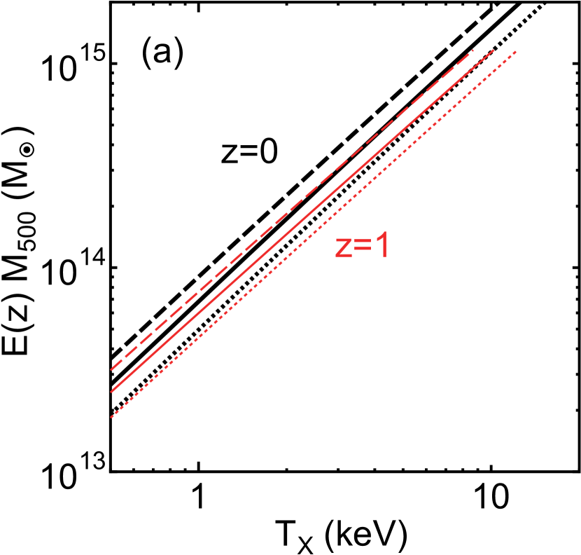
For a given $z$ and $\Delta$, the $M_{\Delta}$–$T_{X}$ relation can be obtained as follows. The mass $M_{\Delta}$ is converted to $M_{s}$ by equation (9) and $c_{\Delta}(M_{\Delta},z)$. The radius $r_{\Delta}$ is a function of $M_{\Delta}$ (equation (6)), and it is converted to $r_{s}$ by equation (3) and $c_{\Delta}(M_{\Delta},z)$. Here, we use the analytically derived FP (equation (4)). Thus, the temperature is given by

$$T_{X}=T_{X0}\left(\frac{r_{s}}{r_{s0}}\right)^{-2}\left(\frac{M_{s}}{M_{s0}}\right)^{(n+11)/6}\>,$$ (11)

where $(r_{s0},M_{s0},T_{X0})$ correspond to a representative point on the FP. Since the similarity solution does not predict $(r_{s0},M_{s0},T_{X0})$, we adopt the logarithmic mean of the parameters for the MUSIC simulation sample; $r_{s0}=414$ kpc, $M_{s0}=1.4\times 10^{14}\>M_{\odot}$, and $T_{X0}=3.7$ keV (Table 1, see also Figure 2). The MUSIC simulation set that we consider is from non-radiative runs and includes 402 clusters at $z=0.25$ with $M_{200}>2\times 10^{14}\>h^{-1}\>M_{\odot}$ (Paper I, see also Meneghetti et al., 2014). Assigning $r_{s}$ and $M_{s}$ in equation (11), we finally obtain the $M_{\Delta}$–$T_{X}$ relation. Numerical simulations have shown that the $c_{\Delta}$–$M_{\Delta}$ relation has an intrinsic scatter of $\sim 0.1$ dex at $M_{200}\sim 10^{14}$–$M^{15}\>\rm M_{\odot}$ (Bullock et al., 2001; Duffy et al., 2008; Ludlow et al., 2013; Meneghetti et al., 2014; Correa et al., 2015). Thus, we also calculate the $M_{\Delta}$–$T_{X}$ relations when $c_{\Delta}$ (fiducial) is replaced by $c_{\Delta}^{U}=10^{0.1}c_{\Delta}$ (upper limit) or $c_{\Delta}^{L}=10^{-0.1}c_{\Delta}$ (lower limit). In the cluster mass range the scatter of the relation is not particularly sensitive to the baryonic physics or to the fitting radial range. In fact, Rasia et al. (2013) found an intrinsic scatter of $\sim$0.1 dex for the relations obtained from simulations both with and without AGN feedback (Tables 1 and 2 of Rasia et al. 2013). Figure 1 shows the relation $M_{\Delta}$–$T_{\Delta}$ for $\Delta=500$ at $z=0$ and 1. We adopt $n=-2$ for Figure 1(a). The slope of the lines at $1\lesssim T_{X}\lesssim 7$ keV is $\alpha=1.33$ for $z=0$ ($E(z)M_{500}\propto T_{X}^{\alpha}$). The values are close to $3/2$ or $1.5$, and $c_{\Delta}^{U}$ gives smaller $M_{500}$ than $c_{\Delta}^{L}$. This relation holds even when $\Delta=200$ and 2500. We emphasize that we did not use the assumption of virial equilibrium when we derive the relation. The figure also shows that the vertical dispersion of the relations should be within a factor of two. The slight difference of the obtained slope $\alpha$ from $1.5$ may be due to some simplified assumption we made when we derived the plane angle. For example, equation (4) is exactly correct only for the Einstein–de Sitter universe because it is based on a similarity solution. For the $\Lambda$CDM cosmology we adopted, the angle of the plane could slightly change (Bertschinger, 1985; Paper I, see also Shi, 2016a).

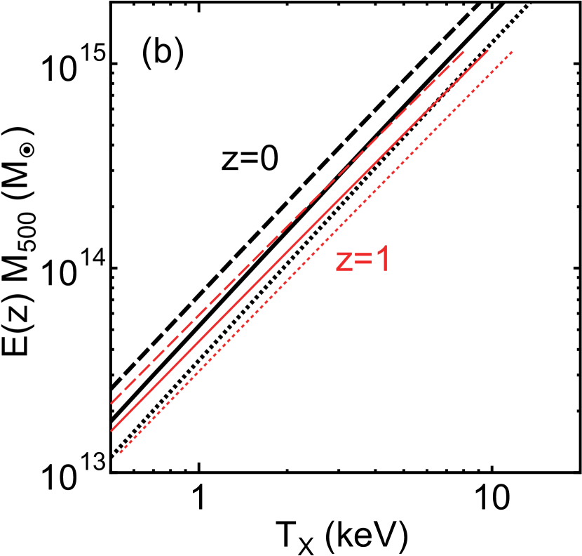
In fact, the slope of $\alpha\sim 1.5$ can be obtained if we change the plane angle only slightly. Figure 1(b) is the same as Figure 1(a) but for $n=-2.5$ in equation (4). While the plane angle is almost the same as that for $n=-2$ (Table 1) and is consistent with the observations (see Figure 4), the slope of the lines is $\alpha=1.53$ for $z=0$. Thus, an imperceptible modification of the angle is enough to obtain $\alpha\sim 1.5$. We also note that the power spectrum index $n$ is expected to be smaller at smaller scales. For example, $n\sim-2.5$ is expected at group scales ($M_{200}\sim 10^{13}\>M_{\odot}$; e.g. Diemer & Kravtsov 2015). This means that the $M_{\Delta}$–$T_{X}$ relation should become qualitatively steeper toward lower $T_{X}$.

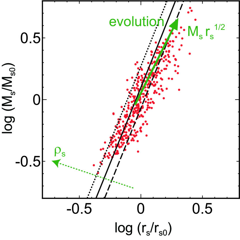
Figure 2 shows the relation between $r_{s}$ and $M_{s}$ at $z=0.25$; they are calculated using $c_{200}(M_{200},z)$. We also plot the data points of the MUSIC simulation (Paper I). For the simulation, the scale radius $r_{s}$ is obtained by fitting the total density distribution (gas+dark matter) with the NFW profile up to $r_{200}$. The mass $M_{s}$ is then derived as the mass enclosed by a sphere of radius $r_{s}$. The figure is similar to Figure 5(a) of Paper I and it is the projection of the FP on the $r_{s}$–$M_{s}$ plane. As can be seen, most of the data points are distributed inside the upper and lower limits of $c_{\Delta}$. This clearly indicates that the dispersion of the $c_{\Delta}$–$M_{\Delta}$ relation corresponds to the spread of the cluster distribution along the minor axis of the FP. Note that the limits along the major axis or the larger and smaller $M_{s}$ limits of the MUSIC data distribution are set by the box size and the resolution of the simulation, respectively. The characteristic density $\rho_{s}$ increases in the direction of the dotted green arrow. Since the three black lines are almost (but not perfectly) perpendicular to the arrow representing the direction of the $\rho_{s}$ axis, the variation of $c_{\Delta}$ is closely related to that of $\rho_{s}$ or the formation time of clusters, although it is not a precise one-to-one correspondence. Individual clusters evolve toward lower $\rho_{s}$ as a whole, but the actual direction (solid green arrow) is mostly determined by the power spectrum of the initial density fluctuations of the universe, and cluster mergers temporally disturb this motion on the FP (Paper I).

Figure 2: Relation between $M_{s}$ and $r_{s}$ at $z=0.25$. The black solid line is calculated for the fiducial $c_{\Delta}$. The black dotted and dashed lines are calculated for $c_{\Delta}^{U}$ and $c_{\Delta}^{L}$, respectively. Individual clusters generally evolve in the direction of the green solid arrow to which the value $M_{s}r_{s}^{1/2}$ increases. The characteristic density $\rho_{s}$ increases and the cluster formation epoch occurs earlier in the direction of the green dotted arrow. Note that the dotted green arrow is almost (but not perfectly) perpendicular to the three parallel black lines. Red dots are the data points of the MUSIC simulation at $z=0.25$, which are the same as those in Figure 5(a) of Paper I.

Figure 3: (a) Points (pin heads) show the distribution of the 44 X-ray clusters in the space of $(\log(r_{s}/r_{s0}),\log(M_{s}/M_{s0}),\log(T_{X}/T_{X0}))$, where $r_{s0}=443$ kpc, $M_{s0}=2.2\times 10^{14}\>M_{\odot}$, and $T_{X0}=7.3$ keV are the sample geometric averages (log means) of $r_{s}$, $M_{s}$, and $T_{X}$, respectively. The length of a pin shows the distance between the point and the obtained plane. The orange plane is translucent and grayish points are located below the plane. The arrow $P_{1}$ shows the direction on the plane in which the data are most extended, and the arrow $P_{2}$ is perpendicular to $P_{1}$ on the plane. The red bars at the corner of the $\log r_{s}$–$\log M_{s}$ plane and on the $\log T_{X}$ axis are typical $1\sigma$ errors of the data. (b) Cross-section of the plane shown in (a). The origin is the same as (a) and $P_{3}$ is the plane normal. The large black points are the X-ray clusters shown in (a). The small red points are the MUSIC-simulated clusters projected on the $P_{1}$–$P_{3}$ plane determined for the X-ray clusters.

Figure 4: The direction of the plane normal $P_{3}=(a,b,c)$ in the space of $(\log r_{s},\log M_{s},\log T_{X})$. Probability contours for the sample of 44 X-ray clusters (black solid lines) are shown at the 68 ($1\>\sigma$), 90, and 99% confidence levels from inside to outside. The prediction of the virial expectation ($r_{s}M_{s}^{-1}T_{X}\propto\rm const$) corresponds to $(\phi,\theta)=(-45^{\circ},55^{\circ})$ (black dot), and is rejected at the 99% confidence level. Probability contours for the CLASH sample (red dotted lines; see Figure 2 of Paper I) are shown for comparison. The plane normal derived for the MUSIC simulation sample is shown by the open red circle; it is located around the 68% contour level and consistent with the X-ray observations at that level. Predictions based on a similarity solution (SSol) for $n=-2$ and $n=-2.5$ are shown by the orange and the blue star, respectively.

4 FP in X-rays

Since X-ray data have shown that the relation $M_{\Delta}\propto T_{X}^{3/2}$ is generally satisfied (Ettori & Fabian, 1999; Neumann & Arnaud, 1999; Nevalainen et al., 2000; Finoguenov et al., 2001; Xu et al., 2001; Vikhlinin et al., 2006), we expect that X-ray data alone form the FP. We will confirm this in this section.

The characteristic radius $r_{s}$ and mass $M_{s}$ can be derived from X-ray data, assuming that the ICM is in hydrostatic equilibrium. Using the X-ray data of 44 clusters obtained with XMM-Newton (Ettori et al. 2010; Table 6), we study their distribution in the space of ($\log r_{s},\log M_{s},\log T_{X}$). The average redshift of the clusters is 0.189. The logarithmic means of $(r_{s},M_{s},T_{X})$ for this sample are $r_{s0}=443$ kpc, $M_{s0}=2.2\times 10^{14}\>M_{\odot}$, and $T_{X0}=7.3$ keV (Table 1). While we adopt the values obtained through method 1 in Ettori et al. (2010), the results are not much different even if we use those obtained through method 2. In Table 6, the X-ray temperatures ($T_{X}$) and masses ($M_{200}$) obtained by Ettori et al. (2010) are listed as $T_{\rm XMM}$ and $M_{\rm 200,XMM}$, respectively. The temperatures are the error-weighted mean of the spectral measurements in the radial range $[0.15\>r_{500},{\rm min}(r_{500},R_{\rm xsp})]$, where $R_{\rm xsp}$ is the maximum radius up to which X-ray spectra can be extracted (see Table 2 of Ettori et al. 2010). This means that $M_{\rm 200,XMM}$ and $c_{200}$ are estimated from the X-ray emission at $\leq r_{500}$. It has been indicated that the temperatures obtained with XMM-Newton tend to be lower than those obtained with Chandra (Nevalainen et al., 2010; Donahue et al., 2014; Israel et al., 2015; Schellenberger et al., 2015; Zhao et al., 2015). Since the temperatures we used for the CLASH sample have been derived with Chandra (Postman et al., 2012), a correction is required to compare the temperatures between the two samples. Ettori et al. (2010) used only MOS1+MOS2, with MOS2 as a value of reference. We convert $T_{\rm XMM}$ in Table 6 into the equivalent Chandra temperature $T_{\rm Ch}$ using the relation,

$$\log\frac{T_{\rm Ch}}{\rm keV}=\frac{1}{A}\left(\log\frac{T_{\rm XMM}}{\rm keV}-B\right)\;,$$ (12)

where $A=0.909^{+0.005}_{-0.005}$ and $B=-0.017^{+0.003}_{-0.004}$ (Schellenberger et al., 2015). Hereafter, we consider $T_{X}$ as the corrected temperature, $T_{\rm Ch}$. Moreover, since cluster mass is estimated based on the temperature, we convert $M_{\rm 200,XMM}$ in Table 6 into the equivalent Chandra mass $M_{\rm 200,Ch}$ using the relation of $M_{\rm 200,Ch}=(T_{\rm Ch}/T_{\rm XMM})M_{\rm 200,XMM}$ and we refer to $M_{\rm 200,Ch}$ as $M_{200}$. The correction does not really affect the following results because we discuss the FP in the logarithmic space. We calculate $M_{s}$ from $M_{200}$ and $c_{200}$ using equation (9) assuming that $c_{200}$ is anti-correlated with $r_{s}$ (Figure 2 of Ettori et al. 2010).

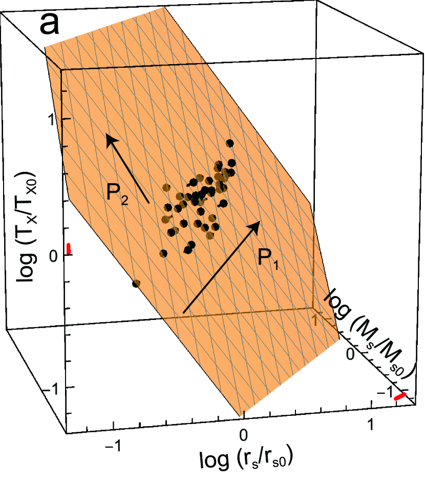
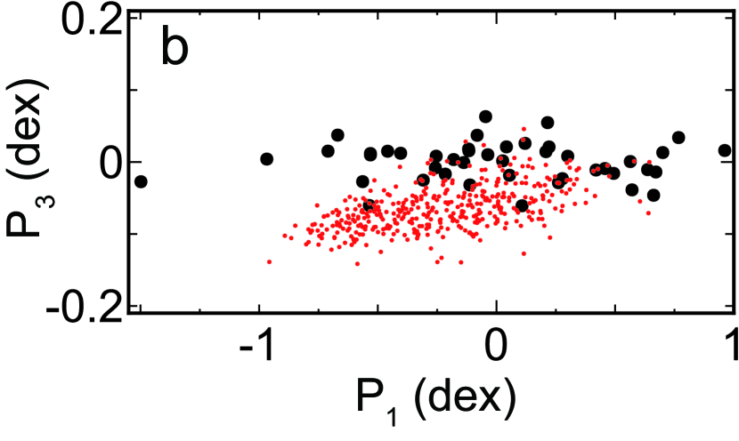
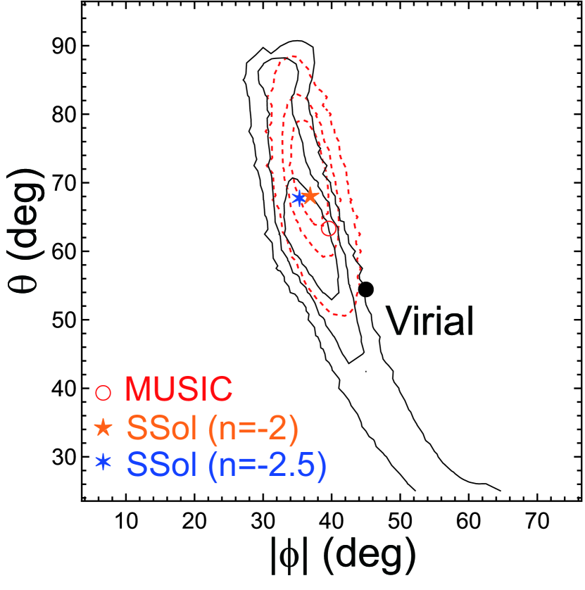
In Figure 3(a), we show the results for the whole sample of 44 clusters; the data points have a planar distribution. The cross section of the plane is shown in Figure 3(b). In this figure, we project the simulated MUSIC clusters on the cross section of the X-ray cluster plane for comparison. The distribution of the MUSIC clusters is slightly deviated from that of the X-ray clusters. We will discuss the absolute position of the X-ray cluster plane in Section 5. We determine the direction of the X-ray cluster plane and the errors through a PCA and Monte-Carlo realizations (see Paper I). The direction on the plane in which the data are most extended is $P_{1}$, and the direction perpendicular to $P_{1}$ on the plane is $P_{2}$. The plane is described by $a\log r_{s}+b\log M_{s}+c\log T_{X}=\mathrm{const.}$, with $a=0.71^{+0.06}_{-0.10}$, $b=-0.53^{+0.02}_{-0.01}$, and $c=0.46^{+0.13}_{-0.11}$. The values of $(a,b,c)$ are consistent with those for the CLASH sample within the errors (Table 1). The thickness of the plane or the dispersion in the direction of $P_{3}$ is $0.039^{+0.021}_{-0.010}$, which is slightly smaller than, but consistent within the errors with the CLASH result (Paper I). Here we note that lensing measurements are sensitive to projection effects, and NFW fitting based on the assumption of spherical symmetry can introduce a sizable scatter in the derived mass and concentration parameters, or $(r_{s},M_{s})$. In our error analysis of the CLASH lensing data (Umetsu et al., 2016), we properly accounted for the projection effects due to cluster halo triaxiality and uncorrelated large-scale structure projected along the line of sight (Gruen et al., 2015), implying that the thickness of the FP derived from our CLASH data should not be affected by the external scatter introduced by the lensing projection effects. The X-ray sample has a wider range of $r_{s}$ and $M_{s}$ compared with the CLASH sample (Figure 1 in Paper I). Since the errors of $a$, $b$, and $c$ are not independent of each other, we show in Figure 4 the likelihood contours of the parameters describing the direction of the plane normal $P_{3}$ for the X-ray sample (black solid lines). In that figure, $\theta$ is the angle between $P_{3}$ and the $\log T_{X}$ axis, and $\phi$ is the azimuthal angle around the $\log T_{X}$ axis, measured anti-clockwise from the $\log r_{s}$ axis, or $\tan\phi=b/a$ (Table 1). The contours are elongated in the direction of rotation around $P_{1}$ (Figure 3(a)), to which the direction $P_{3}$ is less constrained. The contours show that the direction of $P_{3}$ is consistent with that for the CLASH sample (red dotted lines; see Paper I). As long as clusters are widely distributed on the plane, the direction of $P_{3}$ should not be too affected by a possible sample selection bias. In Figure 4, we also plotted MUSIC simulation results (see Paper I for details) and the prediction of the similarity solution (SSol), which is given by equation (4) with $n=-2$ and $-2.5$. They are the same as those in Figure 2 of Paper I and are consistent with the X-ray data at the $\sim 1\>\sigma$ level. For the virial expectation, the angle $\theta$ is the one between vectors $(1/\sqrt{3},-1/\sqrt{3},1/\sqrt{3})$ and $(0,0,1)$, which is $\approx 55^{\circ}$. The prediction of the virial expectation is rejected at the 99% confidence level.

In Paper I, using the results of numerical simulation, we showed that the plane parameters are not very dependent on the relaxation state of clusters, although irregular clusters tend to slightly increase the scatter of the FP. That is, although the cluster parameters ($r_{s}$, $M_{s}$, $T_{X}$) can fluctuate substantially, especially during major mergers, the particular combination of these parameters that determines the FP (e.g. the left side of equation 4) can remain nearly constant. As a result, clusters evolve along the FP and do not much deviate from the FP even during a cluster merger (Section 5.2 in Paper I). Here, we study this issue using the X-ray sample. Ettori et al. (2010) classified the X-ray sample into 18 cool-core (CC) clusters, 19 non-cool-core (NCC) clusters, and 7 intermediate cool-core (ICC) clusters based on the entropy of the ICM in the central region. The CC and NCC clusters tend to be regular and irregular in shape, respectively. We performed the FP analysis for the CC and ICC+NCC samples separately and the results are shown in Table 1. The plane directions are not much different from that of the whole sample of 44 clusters. The thickness of the plane is $0.026^{+0.014}_{-0.006}$ for CC and $0.043^{+0.019}_{-0.010}$ for ICC+NCC, which can be compared with the one for the whole sample ($0.039^{+0.021}_{-0.010}$). Since $r_{s}$ is generally much larger than the cluster core, the details of the ICM physics in the core region are not expected to significantly affect the global cluster parameters, $(\log r_{s},\log M_{s},\log T_{X})$. Although the thicknesses of the planes for the different subsamples are consistent with each other within errors, CC (ICC+NCC) clusters may give a smaller (larger) dispersion about the plane. We note that while the size of the ICC sample alone is too small to reliably determine their FP parameters, the thickness of the plane is slightly increased by including the ICC sample compared to the NCC-only case.

5 Shift of the planes and mass calibration

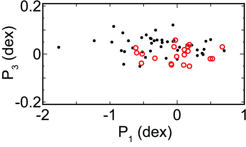
Figure 5 shows the cross sections of the FPs for the CLASH and X-ray samples depicted on the same plane coordinate. Although they overlap with each other, the FP for the CLASH sample (CFP) is located slightly above the FP for the X-ray sample (XFP). Fixing the angles of both planes to the same one given by equation (4) with $n=-2$ (SSol in Table 1), we estimate the distance between the two FPs and find that it is $d_{\rm FP}=0.031^{+0.027}_{-0.039}$ dex in the space of $(\log r_{s},\log M_{s},\log T_{X})$. Thus, the shift of the two planes is not significant. The error of the distance mostly comes from the observational errors of the X-ray data, which result in the uncertainty of the position of the XFP.

Figure 5: The cross-section of the CFP (red circles) and the XFP (black dots). The coordinates $P_{1}$ and $P_{3}$ are for the CFP.

However, X-ray data will be enriched and the configuration of the FP could be determined much more precisely in the near future. In principle, the FP can be used as a benchmark of data calibration, because numerical simulations have shown that the FP is very thin and its origin has been explained by the similarity solution (Paper I). Here, we demonstrate that a possible shift of the FP could be used to calibrate cluster masses $M_{\Delta}$ obtained with X-ray observations. It would be useful even for studies of cluster number counts based on masses estimated by the Sunyaev-Zel’dovich effect, because this estimation relies on X-ray data for calibration (Planck Collaboration et al., 2014). In the following, we use the current observational datasets, although they may not be accurate enough for our calibration purposes.

We study the shift of the XFP against the CFP assuming that the shift is caused by some observational systematic errors. Given the fairly large statistical uncertainties, and for the sake of simplicity, the angles of both FPs are fixed (SSol for $n=-2$ in Table 1), because the direction is consistent with both the CFP and XFP (Figure 4) and the distance between two planes can be well defined only when the planes are parallel. If the data quality and size are improved in the future, this constraint may not be needed. Since both FPs use X-ray data for the temperature, and since the temperature has been corrected by equation (12), we assume that there is no systematic error for temperature, for simplicity. In that case, the shift of the planes may be attributed to the systematic error of $M_{s}$ and/or $r_{s}$. The errors of $M_{s}$ and $r_{s}$ may come from the assumption of hydrostatic equilibrium and the limited radial range adopted in X-ray analysis, respectively (e.g. Nagai et al., 2007; Rasia et al., 2013). First, let us assume that the XFP is shifted solely in the direction of $M_{s}$. In this case, the positions of a given cluster on the CFP and the XFP are given by $(r_{s},M_{sC},T_{X})$ and $(r_{s},M_{sX},T_{X})$, respectively. From now on, we shall use subscript $C$ or $X$ if the value is specifically related to the CFP or the XFP, respectively. Since the two FPs are parallel, the ratio $f_{Ms}\equiv M_{sX}/M_{sC}$ is not unity but is independent of clusters. However, the ratio of $M_{\Delta}$ among the two FPs or $f_{M\Delta}\equiv M_{\Delta X}/M_{\Delta C}$ can vary because $M_{\Delta}$ is a function of $c_{\Delta}$ (equation (9)) that is not constant among clusters. In the Appendix A, we show that $f_{M\Delta}$ is represented by a function of $c_{\Delta X}$ (equation A3) or $c_{\Delta C}$ (equation A4) for a given $f_{Ms}$. Second, let us assume that the XFP is shifted solely in the direction of $r_{s}$. In this case, the positions of a given cluster on the CFP and the XFP are given by $(r_{sC},M_{s},T_{X})$ and $(r_{sX},M_{s},T_{X})$, respectively. The ratio $f_{rs}\equiv r_{sX}/r_{sC}$ is not unity but is independent of clusters. For the second case, we can also derive $f_{M\Delta}$ as a function of $c_{\Delta X}$ (equation A5) or $c_{\Delta C}$ (equation A6) for a given $f_{rs}$.

Figure 6: Relation between $f_{M\Delta}$ and $c_{\Delta X}$. The thick black lines are derived from equation (A3) and thin red lines are derived from equation (A5). The solid lines are for the most certain values of $f_{Ms}$ (thick black) or $f_{rs}$ (thin red). The dashed-dotted lines show the uncertainties attributed to those of $f_{Ms}$ (thick black) or $f_{rs}$ (thin red).

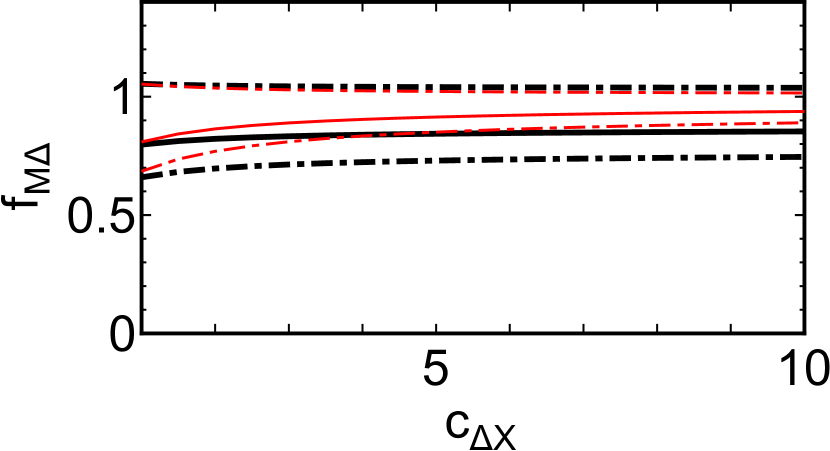
Figure 6 shows the relation between $f_{M\Delta}$ and $c_{\Delta X}$ for our CLASH and X-ray samples. The results do not depend on the value of $\Delta$. Since we assumed that the normal of the two FPs is given by equation (4) for $n=-2$, it is written as ${P_{3}}=(a,b,c)=(0.74,-0.56,0.37)$ (SSol in Table 1). If the shift of the FP is caused by a systematic error of $M_{s}$, we have $f_{Ms}=10^{d_{\rm FP}/b}=0.88^{+0.15}_{-0.09}$. Thus, $f_{M\Delta}$ can be derived from equation (A3), which is shown by the thick black lines in Figure 6. On the other hand, if the shift of the FP is caused by a systematic error of $r_{s}$, we have $f_{rs}=10^{d_{\rm FP}/a}=1.10^{+0.10}_{-0.12}$. Thus, $f_{M\Delta}$ is derived from equation (A5), which is shown by the thin red lines in Figure 6. The $f_{Ms}$–$c_{\Delta C}$ relation is almost the same as the $f_{Ms}$–$c_{\Delta X}$ relation.

Figure 6 shows that $f_{M\Delta}$ does not much depend on $c_{\Delta X}$ and the dependence can be ignored, given the accuracy of the current observations. The dashed-dotted lines suggest that the uncertainty caused by the error of $f_{Ms}$ (black dashed-dotted lines) is larger than that caused by the error of $f_{rs}$ (red dashed-dotted lines). The actual uncertainty should be between the two. If we conservatively adopt the former, $f_{M\Delta}=M_{\Delta X}/M_{\Delta C}\sim 0.85_{-0.2}^{+0.2}$, which means that the mass estimated from the X-ray data may be systematically underestimated compared with that estimated from the CLASH data, but the evidence is not solid. The value of $f_{M\Delta}$ we obtained is consistent with that predicted by numerical simulations (Nagai et al., 2007; Piffaretti & Valdarnini, 2008; Laganá et al., 2010; Rasia et al., 2012). Future improvements of observational data, especially X-ray data, are desired to make a firm conclusion. For the analysis of those data, the dependence of $f_{M\Delta}$ on $c_{\Delta}$ will need to be taken into account. The direction of the plane shift could be determined if $r_{s}$ and $M_{s}$ of certain clusters were precisely determined from both X-ray and gravitational lensing observations. Mock observations of simulated clusters would also be useful to study the shift. Possible differences in the angles of the CFP and the XFP could be a clue for identifying the origin of the observational systematic errors. It would also be interesting to compare the XFPs obtained with different instruments (e.g. Chandra and XMM-Newton) for calibration including $T_{X}$.

6 Summary

We have investigated the origin of the mass–temperature relation of galaxy clusters. Observations and numerical simulations have shown that the relation is approximately represented by $M_{\Delta}\propto T_{X}^{3/2}$ (e.g. $\Delta=500$). This relation has been interpreted as evidence that clusters are in virial equilibrium within $r_{\Delta}$. However, the existence of the FP of clusters and its interpretation based on the modern inside-out scenario suggest that clusters are not in virial equilibrium in the whole region within $r_{\Delta}$ and that the temperatures of clusters are primarily determined by the characteristic mass $M_{s}$ and radius $r_{s}$ of the NFW profile rather than $M_{\Delta}$. We have solved this discrepancy by combining the FP with the concentration–mass–redshift relation of cluster halos calibrated by $N$-body simulations. The relation $M_{\Delta}\propto T_{X}^{3/2}$ is derived from the FP relation among $r_{s}$, $M_{s}$, and $T_{X}$ using the mass dependence of $c_{\Delta}$. We also showed that the dispersion of the $c_{\Delta}$–$M_{\Delta}$ relation can largely account for the spread of the cluster distribution on the FP. Moreover, we confirmed that the FP constructed from X-ray data alone is consistent with that from gravitational lensing data. The FP could be used to calibrate the cluster parameters derived with different methods. As an example, we demonstrated that a cluster mass derived from X-ray observations is systematically $\sim 85_{-20}^{+20}$ % of that derived from gravitational lensing observations.

Table 1: Plane parameters

Sample	$a$	$b$	$c$	$\phi$	$\theta$	$r_{s0}$	$M_{s0}$	$T_{X0}$
				(degree)	(degree)	(kpc)	($10^{14}\>M_{\odot}$)	(keV)
CLASH (CFP)	$0.76^{+0.03}_{-0.05}$	$-0.56^{+0.02}_{-0.02}$	$0.32^{+0.10}_{-0.09}$	-37	71	570	3.8	8.2
SSol ($n=-2$)	0.74	-0.56	0.37	-37	68	$\cdots$	$\cdots$	$\cdots$
SSol ($n=-2.5$)	0.76	-0.54	0.38	-35	68	$\cdots$	$\cdots$	$\cdots$
Virial	0.58	-0.58	0.58	-45	55	$\cdots$	$\cdots$	$\cdots$
MUSIC	0.69	-0.57	0.44	-40	64	414	1.4	3.7
X-ray (XFP)	$0.71^{+0.06}_{-0.10}$	$-0.53^{+0.02}_{-0.01}$	$0.46^{+0.13}_{-0.11}$	-37	63	443	2.2	7.3
X-ray (CC)	$0.72^{+0.04}_{-0.09}$	$-0.52^{+0.02}_{-0.01}$	$0.45^{+0.12}_{-0.05}$	-36	63	529	2.7	7.1
X-ray (ICC+NCC)	$0.69^{+0.10}_{-0.07}$	$-0.53^{+0.03}_{-0.02}$	$0.49^{+0.10}_{-0.23}$	-37	61	392	1.9	7.5

Note. — The vector $(a,b,c)$ is the plane normal $P_{3}$. $\theta$ is the angle between $P_{3}$ and the $\log T_{X}$ axis, and $\phi$ is the azimuthal angle around the $\log T_{X}$ axis. The parameters $(r_{s0},M_{s0},T_{X0})$ represent the (logarithmic) sample means of $(r_{s},M_{s},T_{X})$.

Table 2: Cluster X-Ray data

Cluster	$z$	$r_{s}$	$c_{200}$	$M_{\rm 200,XMM}$	$M_{\rm 200,Ch}$	$T_{\rm XMM}$	$T_{\rm Ch}$
		(kpc)		($10^{14}\>M_{\odot}$)	($10^{14}\>M_{\odot}$)	(keV)	(keV)
RXCJ 0003.8+0203	0.092	$143^{+36}_{-28}$	$8.06^{+1.52}_{-1.30}$	$1.90\pm 0.23$	$2.28^{+0.28}_{-0.28}$	$4.0\pm 0.3$	$4.8^{+0.4}_{-0.4}$
Abell 3911	0.097	$261^{+108}_{-59}$	$5.59^{+1.33}_{-1.39}$	$3.88\pm 0.50$	$4.77^{+0.62}_{-0.63}$	$5.1\pm 0.7$	$6.2^{+1.0}_{-0.9}$
Abell 3827	0.098	$390^{+89}_{-64}$	$4.47^{+0.67}_{-0.64}$	$6.61\pm 0.73$	$8.37^{+0.93}_{-0.93}$	$6.8\pm 0.3$	$8.6^{+0.4}_{-0.4}$
RXCJ 0049.4-2931	0.108	$71^{+30}_{-19}$	$12.78^{+3.80}_{-3.18}$	$0.94\pm 0.16$	$1.10^{+0.19}_{-0.19}$	$3.3\pm 0.8$	$3.8^{+1.0}_{-1.0}$
Abell 2034	0.113	$979^{+7}_{-317}$	$2.46^{+0.81}_{-0.06}$	$17.64\pm 2.17$	$22.18^{+2.76}_{-2.78}$	$6.4\pm 0.9$	$8.0^{+1.3}_{-1.3}$
RXCJ 1516.5-0056	0.115	$563^{+0}_{-114}$	$2.75^{+0.50}_{-0.06}$	$4.73\pm 0.42$	$5.66^{+0.51}_{-0.52}$	$3.9\pm 0.6$	$4.7^{+0.8}_{-0.8}$
RXCJ 2149.1-3041	0.118	$251^{+41}_{-28}$	$4.79^{+0.43}_{-0.49}$	$2.21\pm 0.21$	$2.63^{+0.26}_{-0.26}$	$3.7\pm 0.3$	$4.4^{+0.5}_{-0.4}$
RXCJ 1516.3+0005	0.118	$185^{+67}_{-42}$	$7.06^{+1.64}_{-1.54}$	$2.84\pm 0.41$	$3.48^{+0.51}_{-0.51}$	$4.9\pm 0.2$	$6.1^{+0.4}_{-0.3}$
RXCJ 1141.4-1216	0.119	$496^{+60}_{-36}$	$3.15^{+0.19}_{-0.24}$	$4.88\pm 0.37$	$5.76^{+0.45}_{-0.45}$	$3.5\pm 0.5$	$4.1^{+0.6}_{-0.6}$
RXCJ 1044.5-0704	0.132	$286^{+23}_{-27}$	$4.56^{+0.34}_{-0.25}$	$2.86\pm 0.18$	$3.41^{+0.22}_{-0.22}$	$3.7\pm 0.3$	$4.4^{+0.4}_{-0.4}$
Abell 1068	0.138	$564^{+66}_{-49}$	$3.02^{+0.20}_{-0.22}$	$6.40\pm 0.48$	$7.73^{+0.61}_{-0.60}$	$4.3\pm 0.9$	$5.2^{+1.2}_{-1.2}$
RXCJ 2218.6-3853	0.138	$597^{+184}_{-166}$	$3.16^{+0.85}_{-0.55}$	$8.76\pm 1.62$	$10.98^{+2.03}_{-2.05}$	$6.2\pm 0.5$	$7.8^{+0.7}_{-0.7}$
RXCJ 0605.8-3518	0.141	$369^{+47}_{-39}$	$4.10^{+0.34}_{-0.34}$	$4.51\pm 0.36$	$5.49^{+0.44}_{-0.44}$	$4.6\pm 0.3$	$5.6^{+0.4}_{-0.4}$
RXCJ 0020.7-2542	0.142	$473^{+245}_{-154}$	$4.17^{+1.41}_{-1.07}$	$10.03\pm 2.67$	$12.39^{+3.31}_{-3.33}$	$5.5\pm 1.2$	$6.8^{+1.7}_{-1.7}$
Abell 1413	0.143	$287^{+23}_{-32}$	$5.83^{+0.57}_{-0.35}$	$6.12\pm 0.32$	$7.68^{+0.44}_{-0.43}$	$6.3\pm 1.1$	$7.9^{+1.5}_{-1.4}$
RXCJ 2048.1-1750	0.147	$742^{+80}_{-370}$	$2.23^{+1.63}_{-0.21}$	$5.96\pm 1.12$	$7.34^{+1.38}_{-1.39}$	$5.2\pm 0.4$	$6.4^{+0.5}_{-0.5}$
RXCJ 0547.6-3152	0.148	$443^{+253}_{-71}$	$4.10^{+0.59}_{-1.17}$	$7.89\pm 1.51$	$9.90^{+1.89}_{-1.91}$	$6.3\pm 0.3$	$7.9^{+0.5}_{-0.5}$
Abell 2204	0.152	$816^{+137}_{-0}$	$2.81^{+0.02}_{-0.28}$	$15.93\pm 1.20$	$20.48^{+1.59}_{-1.57}$	$8.0\pm 1.0$	$10.3^{+1.4}_{-1.4}$
RXCJ 0958.3-1103	0.153	$872^{+260}_{-183}$	$2.39^{+0.42}_{-0.39}$	$11.94\pm 2.02$	$14.87^{+2.54}_{-2.55}$	$5.8\pm 1.0$	$7.3^{+1.5}_{-1.4}$
RXCJ 2234.5-3744	0.153	$506^{+261}_{-220}$	$4.28^{+2.31}_{-1.16}$	$13.42\pm 4.15$	$17.19^{+5.30}_{-5.34}$	$7.7\pm 1.0$	$9.9^{+1.4}_{-1.4}$
RXCJ 2014.8-2430	0.161	$462^{+59}_{-25}$	$3.86^{+0.15}_{-0.30}$	$7.56\pm 0.53$	$9.52^{+0.68}_{-0.68}$	$6.5\pm 0.6$	$8.2^{+0.8}_{-0.8}$
RXCJ 0645.4-5413	0.167	$380^{+135}_{-89}$	$4.58^{+1.06}_{-0.96}$	$7.08\pm 1.12$	$9.14^{+1.45}_{-1.45}$	$8.4\pm 0.3$	$10.8^{+0.5}_{-0.5}$
Abell 2218	0.176	$243^{+95}_{-79}$	$6.26^{+2.46}_{-1.48}$	$4.76\pm 0.74$	$5.98^{+0.93}_{-0.94}$	$6.3\pm 0.6$	$7.9^{+0.8}_{-0.8}$
Abell 1689	0.183	$211^{+22}_{-19}$	$8.31^{+0.64}_{-0.63}$	$7.36\pm 0.44$	$9.52^{+0.59}_{-0.58}$	$8.5\pm 0.8$	$11.0^{+1.2}_{-1.2}$
Abell 383	0.187	$435^{+95}_{-0}$	$3.40^{+0.03}_{-0.42}$	$4.43\pm 0.37$	$5.33^{+0.45}_{-0.46}$	$4.1\pm 0.3$	$4.9^{+0.4}_{-0.4}$
Abell 209	0.206	$604^{+272}_{-133}$	$3.03^{+0.67}_{-0.77}$	$8.60\pm 1.23$	$10.80^{+1.57}_{-1.57}$	$6.4\pm 1.2$	$8.1^{+1.7}_{-1.6}$
Abell 963	0.206	$377^{+107}_{-83}$	$4.35^{+0.94}_{-0.76}$	$6.17\pm 0.83$	$7.74^{+1.04}_{-1.05}$	$6.2\pm 0.4$	$7.8^{+0.6}_{-0.6}$
Abell 773	0.217	$605^{+408}_{-233}$	$3.27^{+1.49}_{-1.05}$	$10.94\pm 3.12$	$13.92^{+3.96}_{-3.98}$	$7.3\pm 1.0$	$9.3^{+1.4}_{-1.4}$
Abell 1763	0.223	$192^{+194}_{-49}$	$7.50^{+2.30}_{-3.42}$	$4.25\pm 0.74$	$5.39^{+0.94}_{-0.94}$	$6.8\pm 0.4$	$8.7^{+0.5}_{-0.5}$
Abell 2390	0.228	$1258^{+0}_{-95}$	$2.06^{+0.12}_{-0.04}$	$24.71\pm 1.16$	$32.55^{+1.89}_{-1.89}$	$10.4\pm 2.8$	$13.8^{+4.1}_{-4.0}$
Abell 2667	0.230	$993^{+0}_{-48}$	$2.25^{+0.08}_{-0.02}$	$15.88\pm 0.45$	$20.19^{+0.72}_{-0.70}$	$7.1\pm 1.0$	$9.1^{+1.5}_{-1.4}$
RXCJ 2129.6+0005	0.235	$418^{+68}_{-37}$	$3.71^{+0.27}_{-0.38}$	$5.40\pm 0.44$	$6.66^{+0.55}_{-0.55}$	$5.2\pm 0.5$	$6.5^{+0.7}_{-0.7}$
Abell 1835	0.253	$866^{+46}_{-143}$	$2.64^{+0.34}_{-0.09}$	$17.53\pm 1.41$	$22.59^{+1.91}_{-1.88}$	$8.2\pm 1.5$	$10.6^{+2.1}_{-2.1}$
RXCJ 0307.0-2840	0.253	$611^{+297}_{-175}$	$3.15^{+0.88}_{-0.78}$	$10.44\pm 2.39$	$13.03^{+3.01}_{-3.01}$	$6.1\pm 1.5$	$7.7^{+2.1}_{-2.1}$
Abell 68	0.255	$834^{+0}_{-257}$	$2.65^{+0.82}_{-0.06}$	$15.96\pm 1.98$	$20.20^{+2.53}_{-2.55}$	$6.9\pm 1.1$	$8.7^{+1.6}_{-1.5}$
E 1455+2232	0.258	$214^{+26}_{-22}$	$6.33^{+0.53}_{-0.51}$	$3.66\pm 0.29$	$4.47^{+0.36}_{-0.36}$	$4.7\pm 0.5$	$5.7^{+0.7}_{-0.7}$
RXCJ 2337.6+0016	0.273	$332^{+342}_{-154}$	$4.99^{+3.52}_{-2.18}$	$6.81\pm 1.91$	$8.61^{+2.41}_{-2.43}$	$6.7\pm 1.1$	$8.5^{+1.6}_{-1.5}$
RXCJ 0303.8-7752	0.274	$1115^{+14}_{-497}$	$1.85^{+1.04}_{-0.09}$	$13.21\pm 2.33$	$16.40^{+3.27}_{-3.44}$	$7.0\pm 4.1$	$8.9^{+5.9}_{-5.5}$
RXCJ 0532.9-3701	0.275	$278^{+170}_{-98}$	$5.97^{+2.43}_{-1.82}$	$6.88\pm 1.83$	$8.71^{+2.33}_{-2.34}$	$7.0\pm 1.6$	$8.9^{+2.3}_{-2.2}$
RXCJ 0232.4-4420	0.284	$1172^{+0}_{-409}$	$1.80^{+0.66}_{-0.04}$	$14.28\pm 1.91$	$18.37^{+2.48}_{-2.49}$	$8.1\pm 1.4$	$10.4^{+2.0}_{-2.0}$
ZW 3146	0.291	$510^{+61}_{-31}$	$3.37^{+0.15}_{-0.25}$	$7.79\pm 0.49$	$9.85^{+0.63}_{-0.63}$	$6.8\pm 0.5$	$8.5^{+0.7}_{-0.7}$
RXCJ 0043.4-2037	0.292	$186^{+196}_{-81}$	$7.80^{+5.05}_{-3.51}$	$4.70\pm 1.24$	$5.79^{+1.55}_{-1.55}$	$5.5\pm 1.6$	$6.9^{+2.3}_{-2.2}$
RXCJ 0516.7-5430	0.295	$785^{+405}_{-472}$	$2.41^{+2.82}_{-0.75}$	$10.44\pm 2.88$	$13.02^{+3.60}_{-3.62}$	$5.9\pm 1.1$	$7.4^{+1.5}_{-1.4}$
RXCJ 1131.9-1955	0.307	$797^{+494}_{-309}$	$2.43^{+1.16}_{-0.76}$	$11.31\pm 2.50$	$14.06^{+3.23}_{-3.23}$	$6.3\pm 2.6$	$8.0^{+3.6}_{-3.5}$

Note. — $M_{\rm 200,XMM}$ is the mass $M_{200}$ originally obtained with XMM-Newton, and $M_{\rm 200,Ch}$ is the one corrected for the systematic difference of measured temperature between Chandra and XMM-Newton. $T_{\rm XMM}$ is the X-ray temperature originally obtained with XMM-Newton, and $T_{\rm Ch}$ is the corresponding Chandra temperature (equation (12)).

Appendix A The mass ratio between the FP

First, we assume that the XFP is shifted from the CFP solely in the direction of $M_{s}$. From equation (5),

$$M_{s}=4\pi\delta_{c}\rho_{c}r_{s}^{3}(\ln 2-1/2)\>.$$ (A1)

Thus, the ratio $f_{Ms}$ is equivalent to that of $\delta_{c}$ among the XFP and the CFP or $\delta_{cX}/\delta_{cC}$ if $r_{s}$ does not depend on the FPs. If we define $\delta^{\prime}_{c}\equiv\delta_{c}/\Delta$, we have $f_{Ms}=\delta^{\prime}_{cX}/\delta^{\prime}_{cC}$. From equations (7) and (8), the inverse function of $\delta^{\prime}_{c}$ can be defined, which we call $\tilde{c}_{\Delta}(\delta^{\prime}_{c})$. From equations (6) and (3),

$$f_{M\Delta}=\frac{M_{\Delta X}}{M_{\Delta C}}=\left(\frac{r_{\Delta X}}{r_{\Delta C}}\right)^{3}=\left(\frac{c_{\Delta X}}{c_{\Delta C}}\right)^{3}=\left(\frac{c_{\Delta X}}{\tilde{c}_{\Delta}(\delta^{\prime}_{cC})}\right)^{3}=\left(\frac{c_{\Delta X}}{\tilde{c}_{\Delta}(f_{Ms}^{-1}\delta^{\prime}_{cX})}\right)^{3}$$ (A2)

Since $\delta^{\prime}_{cX}=y(c_{\Delta X})$ from equations (7) and (8), we obtain

$$f_{M\Delta}=\left(\frac{c_{\Delta X}}{\tilde{c}_{\Delta}(f_{Ms}^{-1}y(c_{\Delta X}))}\right)^{3}\>,$$ (A3)

which is a function of $c_{\Delta X}$ for a given $f_{Ms}$. It can also be written as

$$f_{M\Delta}=\left(\frac{\tilde{c}_{\Delta}(f_{Ms}\delta^{\prime}_{cC})}{c_{\Delta C}}\right)^{3}=\left(\frac{\tilde{c}_{\Delta}(f_{Ms}y(c_{\Delta C}))}{c_{\Delta C}}\right)^{3}\>,$$ (A4)

and it is a function of $c_{\Delta C}$ for a given $f_{Ms}$.

Second, we assume that the XFP is shifted from the CFP solely in the direction of $r_{s}$. From equation (A1), we obtain $\delta^{\prime}_{cC}/\delta^{\prime}_{cX}=\delta_{cC}/\delta_{cX}=(r_{sX}/r_{sC})^{3}=f_{rs}^{3}$ if $M_{s}$ does not depend on the FPs. From equations (6) and (3),

$$f_{M\Delta}=\left(\frac{r_{\Delta X}}{r_{\Delta C}}\right)^{3}=\left(\frac{c_{\Delta X}r_{sX}}{c_{\Delta C}r_{sC}}\right)^{3}=f_{rs}^{3}\left(\frac{c_{\Delta X}}{\tilde{c}_{\Delta}(\delta^{\prime}_{cC})}\right)^{3}=f_{rs}^{3}\left(\frac{c_{\Delta X}}{\tilde{c}_{\Delta}(f_{rs}^{3}\delta^{\prime}_{cX})}\right)^{3}=f_{rs}^{3}\left(\frac{c_{\Delta X}}{\tilde{c}_{\Delta}(f_{rs}^{3}y(c_{\Delta X}))}\right)^{3}\>,$$ (A5)

which a function of $c_{\Delta X}$ for a given $f_{rs}$. Similarly, we have

$$f_{M\Delta}=f_{rs}^{3}\left(\frac{\tilde{c}_{\Delta}(f_{rs}^{-3}\delta^{\prime}_{cC})}{c_{\Delta C}}\right)^{3}=f_{rs}^{3}\left(\frac{\tilde{c}_{\Delta}(f_{rs}^{-3}y(c_{\Delta C}))}{c_{\Delta C}}\right)^{3}\>,$$ (A6)

and it is a function of $c_{\Delta C}$ for a given $f_{rs}$.

References

- Bhattacharya et al. (2013) Bhattacharya, S., Habib, S., Heitmann, K., & Vikhlinin, A. 2013, ApJ, 766, 32
- Bertschinger (1985) Bertschinger, E. 1985, ApJS, 58, 39
- Bahcall & Cen (1993) Bahcall, N. A., & Cen, R. 1993, ApJ, 407, L49
- Borgani & Kravtsov (2011) Borgani, S., & Kravtsov, A. 2011, Advanced Science Letters, 4, 204
- Bryan & Norman (1998) Bryan, G. L., & Norman, M. L. 1998, ApJ, 495, 80
- Bullock et al. (2001) Bullock, J. S., Kolatt, T. S., Sigad, Y., et al. 2001, MNRAS, 321, 559
- Correa et al. (2015) Correa, C. A., Wyithe, J. S. B., Schaye, J., & Duffy, A. R. 2015, MNRAS, 452, 1217
- Diemer & Kravtsov (2015) Diemer, B., & Kravtsov, A. V. 2015, ApJ, 799, 108
- Donahue et al. (2014) Donahue, M., Voit, G. M., Mahdavi, A., et al. 2014, ApJ, 794, 136
- Duffy et al. (2008) Duffy, A. R., Schaye, J., Kay, S. T., & Dalla Vecchia, C. 2008, MNRAS, 390, L64
- Dutton & Macciò (2014) Dutton, A. A., & Macciò, A. V. 2014, MNRAS, 441, 3359
- Eisenstein & Hu (1998) Eisenstein, D. J., & Hu, W. 1998, ApJ, 496, 605
- Eke et al. (1996) Eke, V. R., Cole, S., & Frenk, C. S. 1996, MNRAS, 282, 263
- Ettori et al. (2002) Ettori, S., De Grandi, S., & Molendi, S. 2002, A&A, 391, 841
- Ettori & Fabian (1999) Ettori, S., & Fabian, A. C. 1999, MNRAS, 305, 834
- Ettori et al. (2010) Ettori, S., Gastaldello, F., Leccardi, A., et al. 2010, A&A, 524, A68
- Finoguenov et al. (2001) Finoguenov, A., Reiprich, T. H., & Böhringer, H. 2001, A&A, 368, 749
- Fujita & Takahara (1999) Fujita, Y., & Takahara, F. 1999, ApJ, 519, L55
- Fujita et al. (2018) Fujita, Y., Umetsu, K., Rasia, E., et al. 2018, ApJ, 857, 118 (Paper I)
- Gruen et al. (2015) Gruen, D., Seitz, S., Becker, M. R., Friedrich, O., & Mana, A. 2015, MNRAS, 449, 4264
- Israel et al. (2015) Israel, H., Schellenberger, G., Nevalainen, J., Massey, R., & Reiprich, T. H. 2015, MNRAS, 448, 814
- Kaiser (1986) Kaiser, N. 1986, MNRAS, 222, 323
- Laganá et al. (2010) Laganá, T. F., de Souza, R. S., & Keller, G. R. 2010, A&A, 510, A76
- Lieu et al. (2016) Lieu, M., Smith, G. P., Giles, P. A., et al. 2016, A&A, 592, A4
- Ludlow et al. (2013) Ludlow, A. D., Navarro, J. F., Boylan-Kolchin, M., et al. 2013, MNRAS, 432, 1103
- Meneghetti et al. (2014) Meneghetti, M., Rasia, E., Vega, J., et al. 2014, ApJ, 797, 34
- Nagai et al. (2007) Nagai, D., Vikhlinin, A., & Kravtsov, A. V. 2007, ApJ, 655, 98
- Nevalainen et al. (2010) Nevalainen, J., David, L., & Guainazzi, M. 2010, A&A, 523, A22
- Nevalainen et al. (2000) Nevalainen, J., Markevitch, M., & Forman, W. 2000, ApJ, 532, 694
- Navarro et al. (1997) Navarro, J. F., Frenk, C. S., & White, S. D. M. 1997, ApJ, 490, 493
- Neumann & Arnaud (1999) Neumann, D. M., & Arnaud, M. 1999, A&A, 348, 711
- Piffaretti & Valdarnini (2008) Piffaretti, R., & Valdarnini, R. 2008, A&A, 491, 71
- Planck Collaboration et al. (2014) Planck Collaboration, Ade, P. A. R., Aghanim, N., et al. 2014, A&A, 571, A20
- Planelles et al. (2015) Planelles, S., Schleicher, D. R. G., & Bykov, A. M. 2015, Space Sci. Rev., 188, 93
- Postman et al. (2012) Postman, M., Coe, D., Benítez, N., et al. 2012, ApJS, 199, 25
- Rasia et al. (2013) Rasia, E., Borgani, S., Ettori, S., Mazzotta, P., & Meneghetti, M. 2013, ApJ, 776, 39
- Rasia et al. (2012) Rasia, E., Meneghetti, M., Martino, R., et al. 2012, New Journal of Physics, 14, 055018
- Reiprich & Böhringer (2002) Reiprich, T. H., & Böhringer, H. 2002, ApJ, 567, 716
- Salvador-Solé et al. (1998) Salvador-Solé, E., Solanes, J. M., & Manrique, A. 1998, ApJ, 499, 542
- Schellenberger et al. (2015) Schellenberger, G., Reiprich, T. H., Lovisari, L., Nevalainen, J., & David, L. 2015, A&A, 575, A30
- Shi (2016a) Shi, X. 2016a, MNRAS, 459, 3711
- Shi (2016b) Shi, X. 2016b, MNRAS, 461, 1804
- Sun et al. (2009) Sun, M., Voit, G. M., Donahue, M., et al. 2009, ApJ, 693, 1142
- Truong et al. (2018) Truong, N., Rasia, E., Mazzotta, P., et al. 2018, MNRAS, 474, 4089
- Umetsu et al. (2016) Umetsu, K., Zitrin, A., Gruen, D., et al. 2016, ApJ, 821, 116
- Vikhlinin et al. (2009) Vikhlinin, A., Kravtsov, A. V., Burenin, R. A., et al. 2009, ApJ, 692, 1060
- Vikhlinin et al. (2006) Vikhlinin, A., Kravtsov, A., Forman, W., et al. 2006, ApJ, 640, 691
- Wechsler et al. (2002) Wechsler, R. H., Bullock, J. S., Primack, J. R., Kravtsov, A. V., & Dekel, A. 2002, ApJ, 568, 52
- Xu et al. (2001) Xu, H., Jin, G., & Wu, X.-P. 2001, ApJ, 553, 78
- Zhao et al. (2009) Zhao, D. H., Jing, Y. P., Mo, H. J., & Börner, G. 2009, ApJ, 707, 354
- Zhao et al. (2015) Zhao, H.-H., Li, C.-K., Chen, Y., Jia, S.-M., & Song, L.-M. 2015, ApJ, 799, 47
- Zhao et al. (2003) Zhao, D. H., Mo, H. J., Jing, Y. P., & Börner, G. 2003, MNRAS, 339, 12