Screening and anti-screening of the pairing interaction in low-density neutron matter

Abstract

We study pairing in low-density neutron matter including the screening interaction due to the exchange of particle-hole and RPA excitations. As bare force we employ the effective low-momentum interaction $V_{\text{low}\,k}$, while the Fermi-liquid parameters are taken from a phenomenological energy density functional (SLy4) which correctly reproduces the equation of state of neutron matter. At low density, we find screening, i.e., pairing is reduced, while at higher densities, we find anti-screening, i.e., pairing is enhanced. This enhancement is mostly due to the strongly attractive Landau parameter $f_{0}$. We discuss in detail the critical temperature $T_{c}$ in the limit of low densities and show that the suppression of $T_{c}$ predicted by Gor’kov and Melik-Barkhudarov can only be reproduced if the cutoff of the $V_{\text{low}\,k}$ interaction is scaled with the Fermi momentum. We also discuss the effect of non-condensed pairs on the density dependence of $T_{c}$ in the framework of the Nozières-Schmitt-Rink theory.

I Introduction

Neutron stars provide a unique laboratory with an interplay of a wide range of phenomena. The physics of the inner crust of neutron stars, where a dilute gas of unbound neutrons coexists with nuclear clusters, is particularly interesting liv-rev . In this work, we focus on the neutron gas, since its superfluid properties are crucial for the understanding of astrophysical observables such as pulsar glitches or neutron-star cooling. Glitches are the observed sudden increase in the rotational frequency of the pulsars, followed by a long relaxation time and usually they are linked to the neutron superfluidity in the inner crust anderson-itoh ; pines-alpar ; haskell-sedrakian , in particular, to the unpinning of the vortices. After the initial rapid cooling via neutrino emissions, the cooling rate of the neutron star is very dependent on the physics of the crust. The superfluidity of the neutrons in the crust of the star strongly suppresses the specific heat and hence influences the cooling rate yakovlev-pethick ; Fortin2010 . In addition, neutron superfluidity allows for novel neutrino emission processes via Cooper pair breaking and formation that affect the cooling rate of the star close to the transition temperature page-lattimer-prakash-steiner .

Even the modelling of uniform matter is theoretically very challenging due to the uncertainties in the nuclear interactions. In neutron stars, the attractive interaction is provided by the two-body interaction, and the most important channels for neutron pairing turn out to be the ${}^{1}S_{0}$ channel at low densities and therefore occuring in the inner crust, while in the core, the neutrons pair in the triplet ${}^{3}P_{2}-{}^{3}F_{2}$ channel. Protons can also pair, although a description of proton superfluidity is complicated by the asymmetry of matter and the resulting coupling of the protons to the denser background gezerlis-pethick-schwenk . In addition to being crucial for the physics of neutron stars, pairing between nucleons plays a very important role in the spectra of finite nuclei, as well as in description of neutron rich nuclei close to the drip line.

A reliable description of pairing at all densities in infinite matter is still an open question, although the superfluidity in stars has been studied since the early work of Migdal migdal and Ginzburg and Kirzhnits ginzburg64 ; ginzburg69 and is needed to explain observations such as the long relaxation time after a glitch baym-pethick-pines-ruderman . For a recent review, the reader is referred to sedrakian2018 . The simplest starting point for the study of pairing is the superfluid gap equation within the BCS approximation that uses the free-space two-nucleon interaction as input and a free spectrum for the single-particle energies. However, there is enough evidence that one needs to go beyond this approximation gezerlis-pethick-schwenk ; dean-jensen ; Srinivas2016 ; Drischler2016 ; Papakonstantinou2017 ; Rios2017 ; Rios2018 . Medium corrections to the single-particle energy and to the free-space interaction change the gap drastically.

In this work, we re-visit the issue of building an induced interaction that will modify the free space two-body interaction responsible for pairing in the ${}^{1}S_{0}$ channel in uniform neutron matter. In the past, several attempts have been made to include medium corrections to the interaction Wambach1993 ; Schulze1996 ; Shen2003 ; Shen2005 ; Cao2006 . Most of these calculations use many-body methods analogous to the well-known example of screening in an electron gas FetterWalecka , subject to various approximations. Because of the exponential dependence of the gap on the interaction, the final results are always affected by the details. In view of the persistent uncertainties, of some mistakes in LABEL:Shen2005 (see LABEL:Cao2006), and of the simplifying approximation made in LABEL:Cao2006 to replace the 3 particle$-$1 hole (3p1h) matrix element entering the induced interaction by its average value, we believe that this problem has not yet been fully solved, even within the given theoretical framework.

As input, we use the free-space renormalized two-body interaction, $V_{\text{low}\,k}$, evolved from the AV₁₈ two-body potential. The same interaction is also used for the 3p1h couplings entering the induced interaction. The main advantage of using $V_{\text{low}\,k}$ is that non-perturbative features present in the bare interaction, such as the short-range repulsion that arises from the hard-core and the repulsive tensor, are softened. The low-momentum effective interaction depends on the renormalization scale (or cutoff) $\Lambda$, while the free-space two-body observables such as scattering phase shifts and energies are independent of $\Lambda$. However, in principle the renormalization group running generates also induced three- and higher-body forces. In addition, in a many-body calculation, one usually resorts to approximations, which may not hold for all situations. Therefore, when only the free-space evolved two-body interaction is used as input in a many-body calculation, the results may depend on the cutoff and this dependence gives not only an estimate of the importance of the missing $3N$ force but also indicates the importance of the missing many-body terms that may become relevant hebeler-schwenk2010 .

For the induced interaction, except at extremely low densities, it is necessary to go beyond the exchange of simple particle-hole excitations. Following LABEL:Cao2006, we sum the particle-hole bubble series (random-phase approximation, RPA) within the Landau approximation and keep only the lowest order ($L=0$) Landau parameters in the particle-hole interaction. In LABEL:Cao2006, as in preceding studies Schulze1996 ; Shen2005 , the Landau parameters were computed microscopically, including the induced interaction in a self-consistent manner (so-called Babu-Brown theory Babu1973 ). However, the resulting Landau parameters, in particular $F_{0}$, were much smaller than what one obtains from phenomenological energy-density functionals such as the Skyrme SLy4 or the Gogny D1N parameterizations, which have both been fitted to the neutron-matter equation of state. Therefore, we follow a more pragmatic but probably more reliable strategy here, namely to determine the Fermi-liquid parameters (Landau parameters and effective mass) directly from these phenomenological interactions.

The medium corrected interaction is then used in the BCS gap equation and the transition temperature is calculated. We note that our results show screening at low densities and anti-screening at high densities. This is different from the results of Cao et al. in LABEL:Cao2006, where they predict screening for all densities. Our results for screening, e.g., Fig. 12, are compatible with Quantum Monte-Carlo (QMC) results Abe2009 ; Gandolfi2008 ; Gezerlis2010 which rule out the extremely strong screening predicted in earlier calculations Wambach1993 . Unfortunately, QMC results are not available in the density range where we find anti-screening.

Apart from the induced interaction, there are other effects that may modify the BCS results for the transition temperature. If the Fermi momentum $k_{F}$ lies approximately between $1/|a|\sim 0.05$ fm^-1 and $1/r_{e}\sim 0.4$ fm^-1, where $a$ is the neutron-neutron ($nn$) scattering length and $r_{e}$ the effective range, neutron matter is in a strong-coupling situation, in which pair correlations appear already in the normal phase and modify the critical temperature $T_{c}$ Nozieres1985 . This effect is crucial for the understanding of the BCS-BEC crossover as it exists in ultracold Fermi gases or in symmetric nuclear matter Jin2010 , where one can pass from Cooper pairs to a Bose-Einstein condensate (BEC) of dimers (deuterons). For a recent review article, see Strinati2018 . The large value of $|a|$ indicates that the $nn$ interaction is almost able to produce a bound state, and in low-density neutron matter the $nn$ Cooper-pair wave function indeed looks almost like a bound-state wave function Matsuo2006 ; Margueron2007 ; Sun2010 . In fact, one can reach a situation similar to the unitary limit, which is the case of a contact interaction with $|a|\to\infty$ (i.e., $1/|a|\ll k_{F}\ll 1/r_{e}$). The relevance of BEC-BCS cross-over physics for the description of dilute neutron matter was pointed out in many works, e.g. Abe2009 ; Gezerlis2010 ; Matsuo2006 ; Margueron2007 ; Sun2010 ; Ramanan2013 .

Note that, although the strong-coupling situation is only reached at densities below $\sim 0.01$ times nuclear saturation density, it is phenomenologically relevant. Neutron matter with such low densities is present between the clusters in the inner crust of neutron stars at average baryon densities just above the neutron-drip density of $\sim 2.5\times 10^{-4}$ fm^-3 Negele1973 ; Baldo2007 . Since in this region the dilute neutron gas fills almost the entire volume, it represents a sizable contribution to the average baryon density even if its density is a few thousand times smaller than the density inside the clusters.

In the unitary limit, the Nozières-Schmitt-Rink (NSR) theory of pair correlations in the normal phase Nozieres1985 predicts a reduction of the transition temperature $T_{c}$ from the BCS result $\sim 0.5\,E_{F}$ ($E_{F}$ being the Fermi energy) to $\sim 0.22\,E_{F}$ Sa-de-Melo1993 . These numbers do not include screening effects, but as shown recently Pisani2018 , the inclusion of screening on top of the NSR effect leads to good agreement with results from experiments with ultracold atoms. In a previous work Ramanan2013 , we had studied neutron matter in the framework of the NSR theory. In the present paper, we will extend that work to see how the NSR correction is changed by the induced interaction.

This paper is organised as follows: in Sec. II, we re-visit the BCS gap equation and set up the induced interaction. The effect of the induced interaction on the transition temperature is discussed in Sec. III. At low densities, one expects a reduction in $T_{c}$ by a factor of $(4e)^{-1/3}$, which is the Gor’kov-Melik-Barkhudarov (GMB) result Gorkov1961 , and this region is studied in detail in Sec. IV. Finally, we turn our attention to the correlations within the NSR approach in Sec. V. A summary of our results is presented in Sec. VI. Some of the details of the calculations have been moved to appendices to facilitate ease of reading. Numerical results for the matrix elements of the screened pairing interaction are provided in the supplemental material suppl .

II Formalism

II.1 Gap equation and induced interaction

In BCS theory, the ${}^{1}S_{0}$ pairing gap $\Delta$ in neutron matter is determined by the gap equation

$$\Delta(k)=-\frac{2}{\pi}\int_{0}^{\infty}\!dq\,q^{2}V_{0}(k,q)\frac{\Delta(q)\tanh\big{(}\frac{E(q)}{2T}\big{)}}{2E(q)}\,.$$ (1)

Here, $V_{0}(k,q)=\langle k|V_{{}^{1}S_{0}}|q\rangle$ denotes the $nn$ interaction in the ${}^{1}S_{0}$ partial wave for in- and outgoing momenta $q$ and $k$, $E_{q}=\sqrt{(\epsilon(q)-\mu)^{2}+\Delta(q)^{2}}$ is the quasiparticle energy with $\epsilon(q)=q^{2}/2m^{*}$, $m^{*}$ is the neutron effective mass, $\mu$ is the effective chemical potential including the mean-field energy shift, and $T$ is the temperature. Except in some range of low densities, neutron matter is in the weak-coupling limit, in the sense that $\Delta(k_{F})\ll\mu$, implying $\mu\approx k_{F}^{2}/2m^{*}$, with the Fermi momentum $k_{F}=(3\pi^{2}\rho)^{1/3}$ determined by the neutron number density $\rho$. Equation (1) with $V_{\text{low}\,k}$ as $nn$ interaction has been solved, e.g., in LABEL:Kuckei2003.

The critical temperature $T_{c}$ is the highest temperature for which Eq. (1) has a non-trivial solution. At $T=T_{c}$, one can neglect $\Delta(q)$ in $E(q)$, so that Eq. (1) reduces to a linear eigenvalue equation

$$\phi(k)=-\frac{2}{\pi}\int_{0}^{\infty}\!dq\,q^{2}V_{0}(k,q)\frac{\tanh\big{(}\frac{\xi(q)}{2T_{c}}\big{)}}{2\xi(q)}\phi(q)\,,$$ (2)

with $\xi(q)=\epsilon(q)-\mu$. We will also write this as $|\phi\rangle=\mathcal{K}|\phi\rangle$. Hence, in order to find $T_{c}$, we diagonalize the integral operator with the kernel

$$\mathcal{K}(k,q)=-V_{0}(k,q)\frac{\tanh\big{(}\frac{\xi(q)}{2T}\big{)}}{2\xi(q)}\,,$$ (3)

and $T_{c}$ is the temperature where the largest eigenvalue is equal to unity. In weak coupling, $T_{c}$ is directly related to the gap at $T=0$ by $T_{c}=0.57\,\Delta_{T=0}(k_{F})$.

It is widely accepted that an important correction to BCS theory consists in adding to the bare interaction in Eq. (1) the contribution of the induced interaction $V_{\text{ind}}$ due to the exchange of density and spin-density fluctuations. In particular, in the weakly interacting limit, this leads to the famous Gor’kov-Melik-Barkhudarov (GMB) correction, which reduces the gap and the critical temperature by approximately a factor of two compared to the BCS result Gorkov1961 . In terms of Feynman diagrams, this correction can be represented as in Fig. 1 (a).

Figure 1: Feynman diagrams representing the induced interaction. The wiggly line in diagram (b) is meant to include the RPA bubble summation.

Note that the dotted interaction lines are meant to represent the antisymmetrized interaction. This is very important since the dominant ${}^{1}S_{0}$ interaction acts only between neutrons of opposite spin and therefore cannot contribute to the shown diagram. However, if the outgoing lines are exchanged in both the interaction vertices, one obtains a diagram to which it contributes.

In nuclear physics, except at extremely low density (see Sec. IV), one is never in a weakly interacting regime. Therefore, the simple particle-hole bubble exchanged in Fig. 1 (a) is modified by the residual particle-hole interaction as shown in Fig. 1 (b). The wiggly line representing the particle-hole interaction is meant to include the RPA bubble summation to all orders.

Throughout this article, “diagram (a)” and “diagram (b)” refer to the diagrams shown in Fig. 1 (a) and (b). When calculating the diagrams, we make the usual approximation to neglect the energy transfer (static approximation) which can be justified by the observation that the most important contribution to pairing comes from scattering of particles near the Fermi surface, so that all in- and outgoing particles have energies close to the Fermi energy $\epsilon_{F}=k_{F}^{2}/2m^{*}$.

II.2 Diagram (a): single-bubble exchange

Let us first discuss the vertices coupling the particles to the particle-hole excitation, represented as dotted lines in Fig. 1. We assume a general (possibly non-local) interaction which is expanded in partial waves. Using the notation of the left part of Fig. 2,

Figure 2: Elements of Feynman diagrams to clarify the notation. Left: particle-particle interaction. Right: particle-hole propagator.

the partial-wave expansion of the interaction reads

$$\langle\bm{\mathrm{k}}_{1},\sigma_{1};\bm{\mathrm{k}}_{2},\sigma_{2}|V|\bm{\mathrm{k}}^{\prime}_{1},\sigma^{\prime}_{1};\bm{\mathrm{k}}^{\prime}_{2},\sigma^{\prime}_{2}\rangle=\\ \sum_{s,m_{s},m^{\prime}_{s}}\sum_{l,l^{\prime},m_{l}}\sum_{j}C_{\frac{1}{2}\sigma_{1}\frac{1}{2}\sigma_{2}}^{sm_{s}}C_{\frac{1}{2}\sigma^{\prime}_{1}\frac{1}{2}\sigma^{\prime}_{2}}^{sm^{\prime}_{s}}C_{lm_{l}sm_{s}}^{jm_{j}}C_{l^{\prime}m^{\prime}_{l}sm^{\prime}_{s}}^{jm_{j}}\\ \times(4\pi)^{2}i^{l^{\prime}-l}Y^{*}_{lm_{l}}(\Omega_{\bm{\mathrm{Q}}})Y_{l^{\prime}m^{\prime}_{l}}(\Omega_{\bm{\mathrm{Q}}^{\prime}})\langle Q|V_{sll^{\prime}j}|Q^{\prime}\rangle\,,$$ (4)

with

$$\bm{\mathrm{Q}}=\frac{\bm{\mathrm{k}}_{1}-\bm{\mathrm{k}}_{2}}{2}\,,\quad\bm{\mathrm{Q}}^{\prime}=\frac{\bm{\mathrm{k}}^{\prime}_{1}-\bm{\mathrm{k}}^{\prime}_{2}}{2}\,,$$ (5)

$$m^{\prime}_{l}=m_{l}+m_{s}-m^{\prime}_{s}\,,\quad m_{j}=m_{l}+m_{s}\,.$$ (6)

For the Clebsch-Gordan coefficients, we follow the notation of the book by Varshalovich Varshalovich .

Then it is straight-forward to obtain for the diagram (a) the following expression [the factor $(-1)$ comes from the closed Fermion loop]:

$$V_{a}(q,q^{\prime})=(-1)\frac{1}{4\pi}\sum_{\sigma\sigma^{\prime}}C_{\frac{1}{2}\sigma\frac{1}{2}-\sigma}^{00}C_{\frac{1}{2}\sigma^{\prime}\frac{1}{2}-\sigma^{\prime}}^{00}\int\frac{d\Omega_{\bm{\mathrm{q}}}}{4\pi}\int\frac{d\Omega_{\bm{\mathrm{q}}^{\prime}}}{4\pi}\int\frac{d^{3}p}{(2\pi)^{3}}\,\frac{n(\bm{\mathrm{p}}-\bm{\mathrm{k}})-n(\bm{\mathrm{p}})}{\epsilon(\bm{\mathrm{p}})-\epsilon(\bm{\mathrm{p}}-\bm{\mathrm{k}})}\\ \times\sum_{s_{1}m_{s1}}\sum_{s_{2}m_{s2}}\sum_{l_{1}l^{\prime}_{1}m_{l1}}\sum_{l_{2},l^{\prime}_{2},m_{l2}}\sum_{j_{1}j_{2}}C_{\frac{1}{2}\sigma_{1}\frac{1}{2}-\sigma}^{s_{1}m_{s1}}C_{\frac{1}{2}\sigma^{\prime}_{1}\frac{1}{2}-\sigma^{\prime}}^{s_{1}m^{\prime}_{s1}}C_{\frac{1}{2}\sigma\frac{1}{2}\sigma^{\prime}_{1}}^{s_{2}m_{s2}}C_{\frac{1}{2}\sigma^{\prime}\frac{1}{2}\sigma_{1}}^{s_{2}m^{\prime}_{s2}}C_{l_{1}m_{l1}s_{1}m_{s1}}^{j_{1}m_{j1}}C_{l^{\prime}_{1}m^{\prime}_{l1}s_{1}m^{\prime}_{s1}}^{j_{1}m_{j1}}C_{l_{2}m_{l2}s_{2}m_{s2}}^{j_{2}m_{j2}}C_{l^{\prime}_{2}m^{\prime}_{l2}s_{2}m^{\prime}_{s2}}^{j_{2}m_{j2}}\\ \times(4\pi)^{4}i^{l^{\prime}_{1}-l_{1}+l^{\prime}_{2}-l_{2}}Y^{*}_{l_{1}m_{l1}}(\Omega_{\bm{\mathrm{Q}}_{1}})Y_{l^{\prime}_{1}m^{\prime}_{l1}}(\Omega_{\bm{\mathrm{Q}}^{\prime}_{1}})Y^{*}_{l_{2}m_{l2}}(\Omega_{\bm{\mathrm{Q}}_{2}})Y_{l^{\prime}_{2}m^{\prime}_{l2}}(\Omega_{\bm{\mathrm{Q}}^{\prime}_{2}})\langle Q_{1}|\tilde{V}_{s_{1}l_{1}l^{\prime}_{1}j_{1}}|Q^{\prime}_{1}\rangle\langle Q_{2}|\tilde{V}_{s_{2}l_{2}l^{\prime}_{2}j_{2}}|Q^{\prime}_{2}\rangle\,,$$ (7)

with the following abbreviations:

$$\bm{\mathrm{k}}=\bm{\mathrm{q}}-\bm{\mathrm{q}}^{\prime}\,,$$ (8)

$$\begin{split}&\bm{\mathrm{Q}}_{1}=\frac{\bm{\mathrm{q}}+\bm{\mathrm{p}}}{2}\,,\quad\bm{\mathrm{Q}}^{\prime}_{1}=\frac{\bm{\mathrm{q}}^{\prime}-\bm{\mathrm{k}}+\bm{\mathrm{p}}}{2}\,,\\ &\bm{\mathrm{Q}}_{2}=\frac{\bm{\mathrm{q}}+\bm{\mathrm{k}}-\bm{\mathrm{p}}}{2}\,,\quad\bm{\mathrm{Q}}^{\prime}_{2}=\frac{\bm{\mathrm{q}}^{\prime}-\bm{\mathrm{p}}}{2}\,,\end{split}$$ (9)

$$\sigma_{1}=m_{s1}+\sigma\,,\quad\sigma^{\prime}_{1}=m_{s2}-\sigma\,,$$ (10)

$$m^{\prime}_{s1}=m_{s2}-\sigma-\sigma^{\prime}\,,\quad m^{\prime}_{s2}=m_{s1}+\sigma+\sigma^{\prime}\,,$$ (11)

$$m^{\prime}_{l1}=m_{l1}+m_{s1}-m^{\prime}_{s1}\,,\quad m^{\prime}_{l2}=m_{l2}+m_{s2}-m^{\prime}_{s2}\,,$$ (12)

$$m_{j1}=m_{l1}+m_{s1}\,,\quad m_{j2}=m_{l2}+m_{s2}\,.$$ (13)

The tilde in $\tilde{V}$ indicates that the matrix element is antisymmetrized, i.e., multiplied by a factor of two in the surviving channels. For the occupation numbers $n(\bm{\mathrm{p}})$ and $n(\bm{\mathrm{k}}-\bm{\mathrm{p}})$ entering the integral in Eq. (7), we use the step function $n(\bm{\mathrm{p}})=\theta(k_{F}-p)$, which is a very good approximation as long as we are in the weak-coupling limit ($\Delta,T\ll\mu$). Notice that then

$$\lim_{k\to 0}\frac{n(\bm{\mathrm{p}}-\bm{\mathrm{k}})-n(\bm{\mathrm{p}})}{\epsilon(\bm{\mathrm{p}})-\epsilon(\bm{\mathrm{p}}-\bm{\mathrm{k}})}=m^{*}\delta(p-k_{F})\,,$$ (14)

which is useful when evaluating Eq. (7) for $q=q^{\prime}$, especially in the case $q=q^{\prime}=0$.

II.3 Separation of $S=0$ and $S=1$ contributions

It is instructive to split Eq. (7) into contributions from particle-hole excitations having total spin $S=0$ (density waves) and $S=1$ (spin-density waves). In order to do this, consider the particle-hole propagator shown in the right part of Fig. 2, which is given by $G_{0}(p)G_{0}(p-k)\delta_{\sigma_{1}\sigma_{2}}\delta_{\sigma^{\prime}_{1}\sigma^{\prime}_{2}}$ with $G_{0}$ the uncorrelated single-particle Green’s function. This expression appears also in diagram (a) if we formally introduce a summation over $\sigma_{2}$ and $\sigma^{\prime}_{2}$. The spin part can be decomposed using the completeness relation of the Pauli matrices $\bm{\mathrm{\sigma}}$

$$\delta_{\sigma_{1}\sigma_{2}}\delta_{\sigma^{\prime}_{1}\sigma^{\prime}_{2}}=\tfrac{1}{2}(\delta_{\sigma_{1}\sigma^{\prime}_{1}}\delta_{\sigma_{2}\sigma^{\prime}_{2}}+\bm{\mathrm{\sigma}}_{\sigma^{\prime}_{1}\sigma_{1}}\cdot\bm{\mathrm{\sigma}}_{\sigma_{2}\sigma^{\prime}_{2}})\,,$$ (15)

where the two terms correspond, respectively, to $S=0$ and $S=1$. Likewise, this decomposition can also be written in terms of Clebsch-Gordan coefficients as

$$\delta_{\sigma_{1}\sigma_{2}}\delta_{\sigma^{\prime}_{1}\sigma^{\prime}_{2}}=\\ \sum_{S,m_{S}}(-1)^{\frac{1}{2}-\sigma^{\prime}_{1}}C_{\frac{1}{2}\sigma_{1}\frac{1}{2}-\sigma^{\prime}_{1}}^{Sm_{S}}(-1)^{\frac{1}{2}-\sigma^{\prime}_{2}}C_{\frac{1}{2}\sigma_{2}\frac{1}{2}-\sigma^{\prime}_{2}}^{Sm_{S}}\,.$$ (16)

In the calculation of $V_{a}(q,q^{\prime})$, it is clear that in the $S=1$ case each of the three spin projections $m_{S}$ of the particle-hole excitation must give the same contribution. We can therefore compute the $S=1$ contribution by restricting ourselves to the $m_{S}=0$ term, or, equivalently, by keeping only the Pauli matrix $\sigma_{z}$ in the second term of Eq. (15), and multiplying the result by three. This amounts to the replacement

$$\delta_{\sigma_{1}\sigma_{2}}\delta_{\sigma^{\prime}_{1}\sigma^{\prime}_{2}}\to\tfrac{1}{2}\delta_{\sigma_{1}\sigma^{\prime}_{1}}\delta_{\sigma_{2}\sigma^{\prime}_{2}}\left[1+3\,(-1)^{1-\sigma_{1}-\sigma_{2}}\right]\,.$$ (17)

In this way, we arrive at an alternative expression for diagram (a):

$$V_{a}(q,q^{\prime})=(-1)\frac{1}{4\pi}\sum_{\sigma\sigma^{\prime}}C_{\frac{1}{2}\sigma\frac{1}{2}-\sigma}^{00}C_{\frac{1}{2}\sigma^{\prime}\frac{1}{2}-\sigma^{\prime}}^{00}\int\frac{d\Omega_{\bm{\mathrm{q}}}}{4\pi}\int\frac{d\Omega_{\bm{\mathrm{q}}^{\prime}}}{4\pi}\int\frac{d^{3}p}{(2\pi)^{3}}\,\frac{n(\bm{\mathrm{p}}-\bm{\mathrm{k}})-n(\bm{\mathrm{p}})}{\epsilon(\bm{\mathrm{p}})-\epsilon(\bm{\mathrm{p}}-\bm{\mathrm{k}})}\\ \times\sum_{s_{1}m_{s1}}\sum_{s_{2}m_{s2}}\sum_{l_{1}l^{\prime}_{1}m_{l1}}\sum_{l_{2},l^{\prime}_{2},m_{l2}}\sum_{j_{1}j_{2}}C_{\frac{1}{2}\sigma_{1}\frac{1}{2}-\sigma}^{s_{1}m_{s1}}C_{\frac{1}{2}\sigma_{1}\frac{1}{2}-\sigma^{\prime}}^{s_{1}m^{\prime}_{s1}}C_{\frac{1}{2}\sigma\frac{1}{2}\sigma_{2}}^{s_{2}m_{s2}}C_{\frac{1}{2}\sigma^{\prime}\frac{1}{2}\sigma_{2}}^{s_{2}m^{\prime}_{s2}}C_{l_{1}m_{l1}s_{1}m_{s1}}^{j_{1}m_{j1}}C_{l^{\prime}_{1}m^{\prime}_{l1}s_{1}m^{\prime}_{s1}}^{j_{1}m_{j1}}C_{l_{2}m_{l2}s_{2}m_{s2}}^{j_{2}m_{j2}}C_{l^{\prime}_{2}m^{\prime}_{l2}s_{2}m^{\prime}_{s2}}^{j_{2}m_{j2}}\\ \times(4\pi)^{4}i^{l^{\prime}_{1}-l_{1}+l^{\prime}_{2}-l_{2}}Y^{*}_{l_{1}m_{l1}}(\Omega_{\bm{\mathrm{Q}}_{1}})Y_{l^{\prime}_{1}m^{\prime}_{l1}}(\Omega_{\bm{\mathrm{Q}}^{\prime}_{1}})Y^{*}_{l_{2}m_{l2}}(\Omega_{\bm{\mathrm{Q}}_{2}})Y_{l^{\prime}_{2}m^{\prime}_{l2}}(\Omega_{\bm{\mathrm{Q}}^{\prime}_{2}})\langle Q_{1}|\tilde{V}_{s_{1}l_{1}l^{\prime}_{1}j_{1}}|Q^{\prime}_{1}\rangle\langle Q_{2}|\tilde{V}_{s_{2}l_{2}l^{\prime}_{2}j_{2}}|Q^{\prime}_{2}\rangle\\ \times\frac{1}{2}\left[1+3\,(-1)^{1-m_{s1}-m_{s2}}\right]\,,$$ (18)

with the same abbreviations $\bm{\mathrm{k}}$, $\bm{\mathrm{Q}}_{i}$, $\bm{\mathrm{Q}}^{\prime}_{i}$, $m^{\prime}_{li}$, and $m_{ji}$ as before [Eqs. (8), (9), (12), and (13)] but:

$$\sigma_{1}=m_{s1}+\sigma\,,\quad\sigma_{2}=m_{s2}-\sigma\,,$$ (19)

$$m^{\prime}_{s1}=m_{s1}+\sigma-\sigma^{\prime}\,,\quad m^{\prime}_{s2}=m_{s2}-\sigma+\sigma^{\prime}\,,$$ (20)

II.4 Diagram (b): RPA bubble summation

Let us now turn to diagram (b), which includes the RPA bubble summation. In the present work, we will restrict ourselves to the Landau approximation and keep only the lowest-order ($L=0$) Landau parameters. Then the particle-hole interaction takes the form $f+g\,\bm{\mathrm{\sigma}}_{1}\cdot\bm{\mathrm{\sigma}}_{2}$, which allows one to sum the RPA bubble series separately in the $S=0$ and $S=1$ channels. The resulting particle-hole interactions are then

$$f_{\text{RPA}}(k)=\frac{f_{0}}{1-f_{0}\Pi_{0}(k)}\,,\quad g_{\text{RPA}}(k)=\frac{g_{0}}{1-g_{0}\Pi_{0}(k)}\,,$$ (21)

where $f_{0}$ and $g_{0}$ are the Landau parameters for $S=0$ and $S=1$, respectively, and

$$\Pi_{0}(k)=-2\int\frac{d^{3}p}{(2\pi)^{3}}\,\frac{n(\bm{\mathrm{p}}-\bm{\mathrm{k}})-n(\bm{\mathrm{p}})}{\epsilon(\bm{\mathrm{p}})-\epsilon(\bm{\mathrm{p}}-\bm{\mathrm{k}})}$$ (22)

is the static ($\omega\to 0$) limit of the usual Lindhard function $\Pi_{0}(k,\omega)$.

It is convenient to introduce the dimensionless Landau parameters $F_{0}=N_{0}f_{0}$ and $G_{0}=N_{0}g_{0}$, where $N_{0}=m^{*}k_{F}/\pi^{2}$ is the density of states at the Fermi surface (including the neutron-matter degeneracy factor of two), and the dimensionless Lindhard function $\tilde{\Pi}_{0}=\Pi_{0}/N_{0}$. Then, Eq. (21) can be rewritten as

$$f_{\text{RPA}}(k)=\frac{F_{0}/N_{0}}{1-F_{0}\tilde{\Pi}_{0}(k)}\,,\quad g_{\text{RPA}}(k)=\frac{G_{0}/N_{0}}{1-G_{0}\tilde{\Pi}_{0}(k)}\,.$$ (23)

At zero temperature, the Lindhard function can be given in closed form FetterWalecka ,

$$\tilde{\Pi}_{0}(k)=\frac{1}{2}\left[-1+\frac{1-\tilde{k}^{2}/4}{\tilde{k}}\ln\left|\frac{1-\tilde{k}/2}{1+\tilde{k}/2}\right|\right]\,,$$ (24)

with $\tilde{k}=k/k_{F}$.

When computing diagram (b), we use again the trick explained in the derivation of Eq. (18) and compute the $S=1$ contribution as three times the $m_{S}=0$ term, for which $\sigma^{\prime}_{1}=\sigma_{1}$ and $\sigma^{\prime}_{2}=\sigma_{2}$:

$$V_{b}(q,q^{\prime})=\frac{1}{4\pi}\sum_{\sigma\sigma^{\prime}}C_{\frac{1}{2}\sigma\frac{1}{2}-\sigma}^{00}C_{\frac{1}{2}\sigma^{\prime}\frac{1}{2}-\sigma^{\prime}}^{00}\int\frac{d\Omega_{\bm{\mathrm{q}}}}{4\pi}\int\frac{d\Omega_{\bm{\mathrm{q}}^{\prime}}}{4\pi}\int\frac{d^{3}p_{1}}{(2\pi)^{3}}\,\frac{n(\bm{\mathrm{p}}_{1}-\bm{\mathrm{k}})-n(\bm{\mathrm{p}}_{1})}{\epsilon(\bm{\mathrm{p}}_{1})-\epsilon(\bm{\mathrm{p}}_{1}-\bm{\mathrm{k}})}\int\frac{d^{3}p_{2}}{(2\pi)^{3}}\,\frac{n(\bm{\mathrm{p}}_{2}-\bm{\mathrm{k}})-n(\bm{\mathrm{p}}_{2})}{\epsilon(\bm{\mathrm{p}}_{2})-\epsilon(\bm{\mathrm{p}}_{2}-\bm{\mathrm{k}})}\\ \times\sum_{s_{1}m_{s1}}\sum_{s_{2}m_{s2}}\sum_{l_{1}l^{\prime}_{1}m_{l1}}\sum_{l_{2},l^{\prime}_{2},m_{l2}}\sum_{j_{1}j_{2}}C_{\frac{1}{2}\sigma_{1}\frac{1}{2}-\sigma}^{s_{1}m_{s1}}C_{\frac{1}{2}\sigma_{1}\frac{1}{2}-\sigma^{\prime}}^{s_{1}m^{\prime}_{s1}}C_{\frac{1}{2}\sigma\frac{1}{2}\sigma_{2}}^{s_{2}m_{s2}}C_{\frac{1}{2}\sigma^{\prime}\frac{1}{2}\sigma_{2}}^{s_{2}m^{\prime}_{s2}}C_{l_{1}m_{l1}s_{1}m_{s1}}^{j_{1}m_{j1}}C_{l^{\prime}_{1}m^{\prime}_{l1}s_{1}m^{\prime}_{s1}}^{j_{1}m_{j1}}C_{l_{2}m_{l2}s_{2}m_{s2}}^{j_{2}m_{j2}}C_{l^{\prime}_{2}m^{\prime}_{l2}s_{2}m^{\prime}_{s2}}^{j_{2}m_{j2}}\\ \times(4\pi)^{4}i^{l^{\prime}_{1}-l_{1}+l^{\prime}_{2}-l_{2}}Y^{*}_{l_{1}m_{l1}}(\Omega_{\bm{\mathrm{Q}}_{1}})Y_{l^{\prime}_{1}m^{\prime}_{l1}}(\Omega_{\bm{\mathrm{Q}}^{\prime}_{1}})Y^{*}_{l_{2}m_{l2}}(\Omega_{\bm{\mathrm{Q}}_{2}})Y_{l^{\prime}_{2}m^{\prime}_{l2}}(\Omega_{\bm{\mathrm{Q}}^{\prime}_{2}})\langle Q_{1}|\tilde{V}_{s_{1}l_{1}l^{\prime}_{1}j_{1}}|Q^{\prime}_{1}\rangle\langle Q_{2}|\tilde{V}_{s_{2}l_{2}l^{\prime}_{2}j_{2}}|Q^{\prime}_{2}\rangle\\ \times\left[f_{\text{RPA}}(k)+3\,(-1)^{1-m_{s1}-m_{s2}}g_{\text{RPA}}(k)\right]\,,$$ (25)

with the same abbreviations $\bm{\mathrm{k}}$, $\sigma_{i}$, $m^{\prime}_{si}$, $m^{\prime}_{li}$, and $m_{ji}$ as before [Eqs. (8), (19), (20), (12), and (13)] but:

$$\begin{split}&\bm{\mathrm{Q}}_{1}=\frac{\bm{\mathrm{q}}+\bm{\mathrm{p}}_{1}}{2}\,,\quad\bm{\mathrm{Q}}^{\prime}_{1}=\frac{\bm{\mathrm{q}}^{\prime}-\bm{\mathrm{k}}+\bm{\mathrm{p}}_{1}}{2}\,,\\ &\bm{\mathrm{Q}}_{2}=\frac{\bm{\mathrm{q}}+\bm{\mathrm{k}}-\bm{\mathrm{p}}_{2}}{2}\,,\quad\bm{\mathrm{Q}}^{\prime}_{2}=\frac{\bm{\mathrm{q}}^{\prime}-\bm{\mathrm{p}}_{2}}{2}\,,\end{split}$$ (26)

III Anti-screening due to the RPA

III.1 Parameters

For the $nn$ interaction in the particle-particle channel, we use the low-momentum interaction $V_{\text{low}\,k}$ from LABEL:Bogner2007, obtained from the AV₁₈ interaction by a renormalization group evolution (using a smooth Fermi-Dirac regulator with $\epsilon_{\text{FD}}=0.5$) to a final cutoff of $\Lambda=2\,\text{fm}^{-1}$.

For the purpose of comparing with LABEL:Shen2005, we also perform calculations with the Gogny force, using the D1 parameterization Decharge1980 and the more recent D1N parameterization Chappert2008 . For a comparison of the matrix elements of the Gogny force with those of $V_{\text{low}\,k}$, and the corresponding pairing gaps without screening, see LABEL:Sedrakian2003. The explicit expressions for the partial-wave expansion of the Gogny force are given in Appendix A.

Concerning the Fermi-liquid parameters, we do not attempt to compute them from the microscopic theory, but we take more phenomenological results from the SLy4 parameterization of the Skyrme functional Chabanat1997 or from the D1N parameterization of the Gogny force Chappert2008 . The explicit formulas are given in Appendix B, and the resulting Fermi-liquid parameters $m^{*}/m$, $F_{0}$, and $G_{0}$ are shown in Fig. 3.

Figure 3: Fermi-liquid parameters $m^{*}/m$, $G_{0}$, and $F_{0}$ used in the present work, obtained from different phenomenological effective interactions: Skyrme parameterization SLy4 (solid lines), and Gogny D1N (short dashes) and D1 (long dashes) parameterizations.

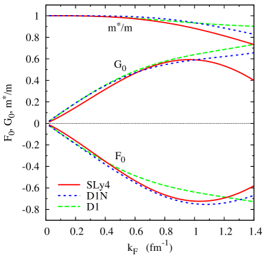
Since both the SLy4 and the D1N effective interactions have been fitted to the neutron-matter equation of state, it is not surprising that they give almost identical results for the Landau parameter $F_{0}$ at low densities. But also the $G_{0}$ values are quite close to each other. Above $k_{F}\sim 1\,\text{fm}^{-1}$, however, the Landau parameters of SLy4 are clearly smaller (in absolute value) than those of D1N. Note also that SLy4 systematically yields a smaller effective mass $m^{*}$ than D1N. For a comparison with LABEL:Shen2005, we also used the D1 parameterization of the Gogny force Decharge1980 , the resulting Fermi-liquid parameters are also shown in Fig. 3.

III.2 Induced interaction

In order to calculate the induced interaction in practice, we restrict the partial-wave expansion in Eq. (4) to some maximum angular momentum, $j\leq j_{\text{max}}$. The multidimensional integrals in Eqs. (7) or (18), and (25) are computed using Monte-Carlo integration. Data files containing tables of the pairing interaction with and without the induced interaction are provided in the supplemental material suppl .

First, we have to check that convergence w.r.t. $j_{\text{max}}$ has been reached. This is indeed the case for $j_{\text{max}}=3$, as can be seen in Fig. 4.

Figure 4: Convergence of the induced interaction with respect to variation of the maximum angular momentum $j_{\text{max}}$ used in the partial wave expansion of the bare interaction. The figure shows the diagonal matrix elements for $k_{F}=0.8\,\text{fm}^{-1}$. Upper thin curves: results for diagram (a), lower thin curves: results for diagram (b), thick curves: sum (a)+(b). The bare interaction in this example is $V_{\text{low}\,k}$, and the Fermi-liquid parameters are those of SLy4.

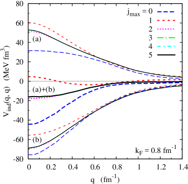
As one can see from this figure, for the example $k_{F}=0.8\,\text{fm}^{-1}$, the net effect of the sum of diagrams (a) and (b) is attractive, i.e., the strong repulsion generated by diagram (a) is more than compensated for by the attractive diagram (b).

This result is in contrast to previous studies Shen2005 ; Cao2006 where it was found that the contribution of diagram (b) is attractive but not strong enough to compensate for the repulsion generated by diagram (a). Let us therefore analyse our result in more detail. It is known that the exchange of $S=0$ excitations (density fluctuations) is attractive and that of $S=1$ excitations (spin-density fluctuations) is repulsive Heiselberg2000 ; Cao2006 . This is also the case in our calculation, as shown in Fig. 5, again for the example $k_{F}=0.8\,\text{fm}^{-1}$.

Figure 5: Induced pairing interaction due to the exchange of $S=0$ (dashed lines) and $S=1$ (dotted lines) excitations. The thin lines represent the contributions of diagrams (a) only, and the thick lines are the sums of diagrams (a) and (b). The thick solid line is the sum of $S=0$ and $S=1$ contributions. The parameters are the same as in Fig. 4.

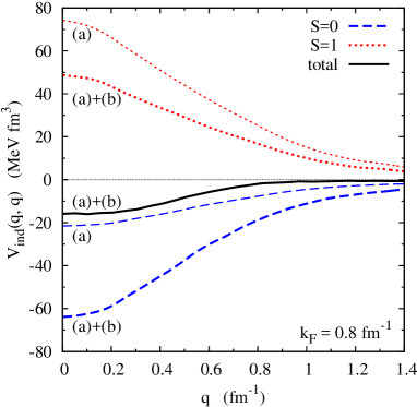
If there was only the single bubble exchange [diagram (a)], the repulsive contribution of $S=1$ excitations would be three to four times larger than the attractive one of $S=0$ excitations. However, the inclusion of the RPA [diagram (b)] acts differently in the cases $S=0$ and $S=1$ because the Landau parameters have opposite signs. In the $S=0$ case, since $F_{0}<0$, the effect of diagram (a) is enhanced, while in the $S=1$ case, since $G_{0}>0$, the effect of diagram (a) is reduced. Therefore, with the inclusion of the RPA, the attraction due to the exchange of density waves can finally win against the repulsive effect of the spin-density waves.

III.3 Critical temperature

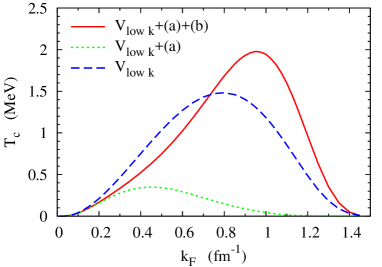
We can now use the induced interaction $V_{\text{ind}}=V_{a}+V_{b}$ and replace the bare interaction $V_{0}$ in the gap equation (1) by $V_{0}+V_{\text{ind}}$. The resulting critical temperature $T_{c}$ as a function of the Fermi momentum $k_{F}$ is shown in Fig. 6.

Figure 6: Critical temperature $T_{c}$ as a function of the Fermi momentum $k_{F}$, obtained with the $V_{\text{low}\,k}$ interaction (Fermi-liquid parameters from the Skyrme force SLy4). Dashes: result obtained using only the bare interaction; dots: result obtained including diagram (a); solid line: full result including also diagram (b).

A sample of the results is also listed in Table 1.

Table 1: Critical temperature as a function of the Fermi momentum $k_{F}$, obtained with $V_{\text{low}\,k}$ interactions and Fermi-liquid parameters from SLy4. $T_{c}^{\text{(bare)}}$ is obtained with the bare interaction, while $T_{c}^{\text{(screened)}}$ includes the effect of $V_{\text{ind}}=V_{a}+V_{b}$. The columns marked $\Lambda=2$ fm^-1 correspond to the parameters given in Sec. III.1, while for the columns marked $\Lambda=2.5\,k_{F}$, a $V_{\text{low}\,k}$ interaction with a density dependent cutoff and a different regulator was used, see Sec. IV.2.

	$\Lambda=2$ fm-1		$\Lambda=2.5\,k_{F}$
$k_{F}$	$T_{c}^{\text{(bare)}}$	$T_{c}^{\text{(screened)}}$	$T_{c}^{\text{(bare)}}$	$T_{c}^{\text{(screened)}}$
(fm-1)	(MeV)	(MeV)	(MeV)	(MeV)
$0.08$	$0.0230$	$0.0211$	$0.0221$	$0.0135$
$0.2$	$0.212$	$0.167$	$0.206$	$0.128$
$0.4$	$0.752$	$0.523$	$0.743$	$0.488$
$0.6$	$1.27$	$1.02$	$1.27$	$1.03$
$0.8$	$1.48$	$1.68$	$1.48$	$1.70$
$1.0$	$1.18$	$1.94$	$1.18$	$1.90$
$1.2$	$0.485$	$0.964$	$0.474$	$0.789$
$1.3$	$0.184$	$0.352$
$1.4$	$0.0323$	$0.0489$

The corresponding pairing gaps $\Delta(k_{F})$ at $T=0$ can be obtained, to a very good approximation, by multiplying $T_{c}$ with 1.76. The dashed line represents the result obtained with the bare interaction $V_{\text{low}\,k}$. The maximum critical temperature is reached at $k_{F}\approx 0.8\,\text{fm}^{-1}$. When one includes the induced interaction due to diagram (a) alone, pairing is very strongly suppressed, as shown by the dotted line. Finally, when including diagrams (a) and (b), one finds that the critical temperature is lowered at low density, but increased at high density. The change from screening to anti-screening is at $k_{F}\approx 0.73\,\text{fm}^{-1}$, consistent with our results discussed in Sec. III.2 where we found that at $0.8\,\text{fm}^{-1}$ the attractive effect of $S=0$ excitations is stronger than the repulsive effect of $S=1$ excitations. Whether the net effect of the induced interaction is attractive (i.e., anti-screening) or repulsive (i.e. screening), depends of course on the density and on the values of the Landau parameters. With decreasing density, the RPA bubbles of diagram (b) become less important and therefore the repulsive effect of diagram (a) wins. This explains why, at very low density, the full result and the result obtained with only diagram (a) become equal, as one can also see in Fig. 6.

To check how sensitive our results are to the details of the model, we repeated the calculation with the D1N and D1 Gogny forces. In these cases, the same interaction is used for the bare pairing force, for the vertices entering the induced interaction diagrams (a) and (b), and for the Fermi-liquid parameters. The results are shown in Fig. 7.

Figure 7: Same as Fig. 6, but here the Gogny D1N and D1 interactions are used in the particle-particle channel and for the Fermi-liquid parameters.

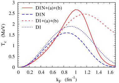
Of course, since the ${}^{1}S_{0}$ matrix elements of the different interactions are not the same, there is already some difference at the level of the bare interaction Sedrakian2003 : the maximum is slightly shifted and the gap survives up to higher density. However, the effect of the induced interaction is qualitatively the same as in Fig. 6, i.e., the gap is reduced at low density and increased at high density. The change from screening to anti-screening happens at about the same density as with $V_{\text{low}\,k}$ (with Fermi-liquid parameters from SLy4) in Fig. 6, and compared to the $V_{\text{low}\,k}$ results the anti-screening effect at high density is even stronger with both the D1N and the D1 Gogny interactions.

IV The low-density limit

As one sees from Fig. 6, with the $V_{\text{low}\,k}$ interaction with a fixed cutoff of $2\,\text{fm}^{-1}$, screening gets weak at low density and finally at $k_{F}\lesssim 0.1\,\text{fm}^{-1}$ one recovers the BCS result. However, at $k_{F}\ll 1/|a|$, the GMB result should be valid, predicting a reduction of $T_{c}$ by a factor of $(4e)^{-1/3}\approx 0.45$. Therefore, let us study the low-density limit in more detail.

IV.1 Failure of the weak coupling formula

As we have seen, the contribution of diagram (b) becomes negligible at low density. Concerning diagram (a), it seems natural to concentrate on matrix elements $V_{a}(q,q^{\prime})$ with $q,q^{\prime}\simeq k_{F}$. If $k_{F}$ becomes small, this means that also $q$ and $q^{\prime}$ and hence all the momenta $Q_{1}$ etc. that appear in Eq. (7) become small. Therefore, we can replace

$$\langle Q_{i}|\tilde{V}_{s_{i}l_{i}l_{i}^{\prime}j_{i}}|Q_{i}^{\prime}\rangle\xrightarrow{q,q^{\prime},k_{F}\to 0}2V_{0}(0,0)\,\delta_{s_{i}0}\,\delta_{l_{i}0}\,\delta_{l_{i}^{\prime}0}\,\delta_{j_{i}0}$$ (27)

(the factor of two accounts for the antisymmetrization of $\tilde{V}$), and Eq. (7) simplifies tremendously to

$$V_{a}(q,q^{\prime})\approx-2\pi N_{0}|V_{0}(0,0)|^{2}\langle\tilde{\Pi}_{0}\rangle\,.$$ (28)

In this expression, we have used the angle-averaged Lindhard function

$$\langle\tilde{\Pi}_{0}\rangle=\frac{1}{2}\int_{-1}^{1}\!d\cos\theta\,\tilde{\Pi}_{0}\big{(}\sqrt{q^{2}+q^{\prime\,2}-2qq^{\prime}\cos\theta}\big{)}\,,$$ (29)

see appendix C. In particular, we get

$$V_{a}(k_{F},k_{F})\approx 2\pi N_{0}|V_{0}(0,0)|^{2}\tfrac{1}{3}\ln 4e\,.$$ (30)

Following well-known weak-coupling arguments FetterWalecka , the gap and critical temperature should be proportional to $e^{1/[2\pi N_{0}V_{0}(k_{F},k_{F})]}$. If we replace $V_{0}$ by $V_{0}+V_{a}$ in the approximation given in Eq. (30), we find that the gap and the critical temperature should indeed be reduced by the factor $(4e)^{-1/3}$, in contradiction to our numerical results which show that at low density $T_{c}$ is not modified at all by screening. Obviously the weak-coupling formula does not apply in the present case, although we are clearly in a weak coupling situation since $T_{c}\ll\epsilon_{F}$. Note that there are a couple of cases in nuclear physics where the weak coupling formula is known to fail Clark2013 .

When using the weak coupling formula, one assumes that the kernel $\mathcal{K}(k,q)$ given in Eq. (3) is sharply peaked at $q=k_{F}$ and that this peak gives the dominant contribution to the integral in the gap equation. However, we will show that the contribution of the peak is not dominant at low density, and this is the reason why the weak coupling formula fails in this case.

Remember that the critical temperature is given by the temperature where the largest eigenvalue $\eta$ of the kernel $\mathcal{K}(k,q)$ given in Eq. (3) is equal to unity. The corresponding eigenvector $|\phi\rangle$ can be found by numerical diagonalization, its representation in momentum space, $\phi(q)=\langle q|\phi\rangle$, is a smooth function of $q$ which has approximately the shape of $V_{0}(q,k_{F})$. If we normalize the eigenvector to $\langle\phi|\phi\rangle=(2/\pi)\int\!dq\,q^{2}|\phi(q)|^{2}=1$, we can write the eigenvalue $\eta$ as

$$\eta=\langle\phi|\mathcal{K}|\phi\rangle=\frac{4}{\pi^{2}}\int\!dq\,q^{2}\int\!dk\,k^{2}\phi(k)\mathcal{K}(k,q)\phi(q)\,.$$ (31)

To measure the importance of the peak of the kernel at $q=k_{F}$, we can look at this integral as a function of its upper limit $q_{\text{max}}$,

$$I_{\eta}(q_{\text{max}})=-\frac{4}{\pi^{2}}\int_{0}^{q_{\text{max}}}dq\,q^{2}\phi(q)\frac{\tanh\big{(}\frac{\xi(q)}{2T}\big{)}}{2\xi(q)}\\ \times\int_{0}^{\infty}dk\,k^{2}\phi(k)V(k,q)\,.$$ (32)

At $T=T_{c}$, we know that $I_{\eta}\to 1$ for $q_{\text{max}}\to\infty$ since $\eta=1$. For the weak coupling formula to be valid, the main contribution to the integral should come from $q\approx k_{F}$, i.e., $I_{\eta}$ should be close to the step function $\theta(q_{\text{max}}-k_{F})$. In Fig. 8

Figure 8: Measure of the contribution of different momenta to the gap equation as defined in Eq. (32), for two different densities ($k_{F}=0.012\,\text{fm}^{-1}$ (solid line) and $1.45\,\text{fm}^{-1}$ (dashes), indicated by the thin vertical lines). The integrals were calculated with the $V_{\text{low}\,k}$ interaction $m^{*}$ from the Skyrme force SLy4) at the respective critical temperatures.

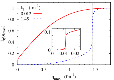
we show the behavior of $I_{\eta}$ for two cases, $k_{F}=1.45\,\text{fm}^{-1}$ (dashes) and $k_{F}=0.012\,\text{fm}^{-1}$ (solid line). In both cases, we are in the weak-coupling limit, in the sense that $T_{c}/E_{F}$ is very small (of the order of $10^{-4}$). In the case $k_{F}=1.45\,\text{fm}^{-1}$, we see that about 80% of the integral come from momenta close to $k_{F}$, so that in this case $T_{c}$ is indeed determined to a large extent by $V(k_{F},k_{F})$. But in the low-density case, $k_{F}=0.012\,\text{fm}^{-1}$, the situation is completely different. Although there is again a sharp rise of $I_{\eta}$ at $q\approx k_{F}$ (visible in the zoom), its contribution to the total integral is less than 10%. The largest contribution to the integral comes from momenta that are considerably larger than $k_{F}$.

Let us now look at the matrix elements $V(q,k_{F})$ for $k_{F}=0.012\,\text{fm}^{-1}$ with and without screening, which are displayed in Fig. 9.

Figure 9: Matrix elements $V(q,k_{F})$ of the bare ($V_{\text{low}\,k}$, dashes) and of the screened (solid line) interaction for $k_{F}=0.012\,\text{fm}^{-1}$. For comparison, we display also the screened interaction obtained with the analytical approximation Eq. (28) (dots, almost indistinguishable from the solid line). The screening correction is so tiny that it is almost invisible on the big graph, see the inset for a zoom. The thin vertical line indicates $q=k_{F}$.

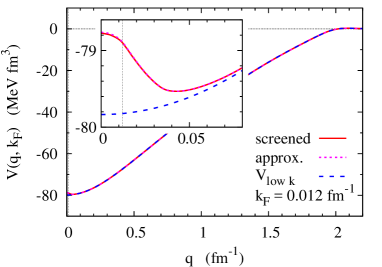
The screening correction is limited to the tiny region $q\lesssim 0.05\,\text{fm}^{-1}\sim 4k_{F}$, because of the strong momentum dependence of the angle-averaged Lindhard function. But as we have seen before, this small region contributes only about 10% to the integral in the gap equation, and therefore the screening correction has practically no effect on the gap or $T_{c}$.

The observation that the screening effect disappears at low density is not a singular feature of our calculation, but it can also be found in the existing literature Cao2006 . However, as we will discuss below, there are other problems with the low-density limit. Taking these into account, we will eventually retrieve the GMB result.

IV.2 Failure of perturbation theory and density-dependent cutoff

When calculating diagrams (a) and (b), we use the bare interaction $V$ perturbatively to describe the vertex coupling the particles to the particle-hole excitations. Since we are using renormalized interactions whose matrix elements decrease rapidly with increasing relative momenta $Q_{i}$ and $Q_{i}^{\prime}$, which are typically of the order of $k_{F}$, this may be a good approximation at higher densities. However, for small $Q_{i}$ and $Q_{i}^{\prime}$, as they appear at low densities, we know from the large value of the $nn$ scattering length $a$ that the perturbative treatment must fail Bogner-nm-2005 ; Bogner-convergence-2006 .

When looking at the historical work by GMB Gorkov1961 , one observes that they compute the correction in a different way. Namely, instead of using the potential $V$ in the dashed interaction vertices of diagram (a), they use $a/m$. This amounts to including, at least approximately, the resummation of ladder diagrams as shown in Fig. 10.

Figure 10: Higher-order ladder diagrams in the 3p1h vertices which are not included in the present work.

In contrast to the Gogny interaction, the renormalization-group evolved $V_{\text{low}\,k}$ interaction gives us the additional freedom to change the cutoff $\Lambda$. On the one hand, by lowering the cutoff, the interaction gets obviously “more perturbative”. In this sense, it is tempting to lower the cutoff as much as possible. In fact, for $q,q^{\prime}<\Lambda$ and $\Lambda\to 0$, the matrix elements get more and more attractive and flow towards the constant $a/m$ as

$$V_{0}(q,q^{\prime})\approx\Big{(}\frac{m}{a}-\frac{2m\Lambda}{\pi}\Big{)}^{-1}\,.$$ (33)

This means that the contribution of higher-order ladder diagrams gets progressively included, via the renormalization group flow, in the two-body matrix elements, while the loop integrals become suppressed, and as a result, it should be possible to work with a Born approximation to the $\mathcal{T}$ matrix at low cutoffs. On the other hand, one of course must not lower the cutoff below the relevant momentum scale of the order of $k_{F}$.

The cutoff dependence of the gap (without screening corrections) was investigated in LABEL:Schwenk2007. Numerically, we obtain cutoff independent results for $T_{c}$ at the BCS level in the whole range of densities for $\Lambda\gtrsim 2.5\,k_{F}$, if we use an exponential regulator of the form $\exp(-(k^{2}/\Lambda^{2})^{n_{\text{exp}}})$ with $n_{\text{exp}}=5$. (With the Fermi-Dirac regulator and with $\epsilon_{\text{FD}}=0.5\,\text{fm}^{-1}$ that we used before we would need somewhat larger cutoffs.)

So, let us see what we find when we choose instead of a constant cutoff $\Lambda=2\,\text{fm}^{-1}$ the lowest possible cutoff for each value of $k_{F}$, i.e., $\Lambda=2.5\,k_{F}$.

As an example, let us consider as in Fig. 9 the case $k_{F}=0.012\,\text{fm}^{-1}$. If we evolve the cutoff to the lowest possible value for this $k_{F}$, i.e., to $\Lambda=2.5\,k_{F}=0.03\,\text{fm}^{-1}$, we obtain the matrix elements $V(q,k_{F})$ shown in Fig. 11.

Figure 11: Same as Fig. 9 but now calculated with an interaction $V_{\text{low}\,k}$ evolved to a much lower cutoff $\Lambda=0.03\,\text{fm}^{-1}=2.5\,k_{F}$ (and with an exponential instead of Fermi-Dirac regulator, see text).

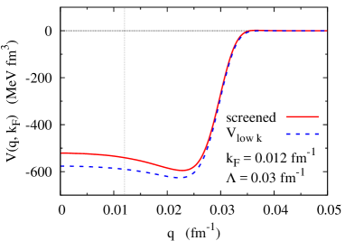
As in Fig. 9, the dashed line represents $V_{\text{low}\,k}$ without screening and the solid line has screening included. The most obvious difference between Figs. 9 and 11 is that, when the cutoff is lowered, the $V_{\text{low}\,k}$ matrix elements (dashed lines) get more attractive, cf. Eq. (33). However, the renormalization group flow does not only ensure that the low-energy scattering in free space remains unchanged, but also the gap and $T_{c}$ at the BCS level (i.e., without screening) remain the same, as mentioned above. But the results with screening change. Now, the modification of the interaction due to screening (difference between the solid and the dashed lines in Fig. 11) extends over the whole momentum range up to $\sim\Lambda$, and therefore the screening will reduce $T_{c}$, contrary to what happened in the case $\Lambda=2\,\text{fm}^{-1}$.

Since the results for $T_{c}$ obtained without the screening correction is the same as the one we obtained before for $\Lambda=2\,\text{fm}^{-1}$, we can concentrate on the correction of $T_{c}$ due to screening. In Fig. 12,

Figure 12: Reduction of the critical temperature due to the screening correction $V_{\text{ind}}=V_{a}+V_{b}$ as a function of $k_{F}$, obtained with the constant cutoff $\Lambda=2\,\text{fm}^{-1}$ (dashes) and with the density-dependent cutoff $\Lambda=2.5\,k_{F}$ (solid line), respectively.

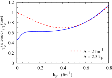
we therefore display the ratio of $T_{c}$ with screening to $T_{c}$ without screening as a function of $k_{F}$. The red dashes correspond to the results shown already in Fig. 6, obtained with a constant cutoff $\Lambda=2\,\text{fm}^{-1}$, and we clearly see that the effect of the screening correction vanishes at low density, as explained in Sec. IV.1. The new results obtained with the variable cutoff $2.5\,k_{F}$ are shown as the blue solid line. We see that now the reduction of $T_{c}$ due to screening survives at low densities, and in the limit $k_{F}\to 0$ it indeed seems to approach the factor $(4e)^{-1/3}\approx 0.45$ predicted by GMB. Note that the original GMB paper Gorkov1961 considers $k_{F}|a|\ll 1$, i.e., in the case of neutron matter, $k_{F}\ll 0.05\,\text{fm}^{-1}$.

V Effect of the Nozières-Schmitt-Rink correction

V.1 Brief summary of the formalism

In our previous work Ramanan2013 , we had studied neutron matter within the NSR approach using only the free-space renormalized effective interaction $V_{0}$. In the present work, we will revisit the inclusion of preformed pairs above $T_{c}$, including the induced interaction $V_{\text{ind}}$ shown in Fig. 1. For the sake of completeness, we summarize briefly the key ideas and formulas of the NSR approach. For more details, we refer the reader to LABEL:Ramanan2013.

Within the NSR approach, for a given chemical potential $\mu$, the density of the interacting neutrons is enhanced by the pair correlations that build up as a precursor effect to the superfluid phase transition already above $T_{c}$. Therefore, the total density of neutrons, $\rho_{\text{tot}}$, can be written as

$$\rho_{\text{tot}}=\rho_{0}+\rho_{\text{corr}}\,.$$ (34)

The uncorrelated neutron density $\rho_{0}$ is given by

$$\rho_{0}=2\int\!\frac{d^{3}k}{(2\pi)^{3}}\,f(\xi(\bm{\mathrm{k}}))\,,$$ (35)

where $f(\xi)=1/(e^{\beta\xi}+1)$ is the Fermi-Dirac distribution function (with $\beta=1/T$) and the factor of $2$ arises due to the spin degeneracy. The correlated density, $\rho_{\text{corr}}$, in the imaginary-time formalism FetterWalecka , is calculated to first order in the single-particle self-energy $\Sigma$ as

$$\rho_{\text{corr}}=2\int\!\frac{d^{3}k}{(2\pi)^{3}}\frac{1}{\beta}\sum_{\omega_{n}}\big{(}\mathcal{G}_{0}(\bm{\mathrm{k}},\omega_{n})\big{)}^{2}\\ \times[\Sigma(\bm{\mathrm{k}},i\omega_{n})-\operatorname{Re}\Sigma(\bm{\mathrm{k}},\xi(\bm{\mathrm{k}}))]\,,$$ (36)

where $\omega_{n}$ are the fermionic Matsubara frequencies and $\mathcal{G}_{0}=1/(i\omega_{n}-\xi(\bm{\mathrm{k}}))$ is the uncorrelated single-particle Green’s function. The subtraction of the on-shell self-energy in the square bracket of Eq. (36) is absent in the original NSR approach. It takes into account the fact that $\mathcal{G}_{0}$ includes already the in-medium quasiparticle energy $\xi(\bm{\mathrm{k}})$ which therefore must not be shifted by the self-energy Zimmermann1985 ; Jin2010 .

Let us consider the first term without the subtraction. $\Sigma(\bm{\mathrm{k}},i\omega_{n})$ is calculated within the ladder approximation, i.e.,

$$\Sigma(\bm{\mathrm{k}},i\omega_{n})=\int\frac{d^{3}K}{(2\pi)^{2}}\frac{1}{\beta}\sum_{\omega_{N}}\mathcal{G}_{0}(\bm{\mathrm{K}}-\bm{\mathrm{k}},\omega_{N}-\omega_{n})\\ \times\big{\langle}\tfrac{\bm{\mathrm{K}}}{2}-\bm{\mathrm{k}}\big{|}\mathcal{T}(\bm{\mathrm{K}},i\omega_{N})\big{|}\tfrac{\bm{\mathrm{K}}}{2}-\bm{\mathrm{k}}\big{\rangle}\,,$$ (37)

where $\mathcal{T}(\bm{\mathrm{K}},i\omega_{N})$ is the in-medium $\mathcal{T}$ matrix for the bosonic Matsubara frequency $\omega_{N}$ and total momentum $\bm{\mathrm{K}}$. The $\mathcal{T}$-matrix is subsequently expanded in a partial wave basis and we pick out only the $s$-wave contribution. Following the steps outlined in Ramanan2013 and analytically continuing to real $\omega$, one obtains for the correlated density within the NSR approach:

$$\rho_{\text{corr},1}=-\frac{\partial}{\partial\mu}\int\!\frac{K^{2}dK}{2\pi^{2}}\!\int\!\frac{d\omega}{\pi}\,g(\omega)\operatorname{Im}\operatorname{Tr}\log\big{(}1-V\overline{G}_{0}^{(2)}\big{)}\,.$$ (38)

Here, $g(\omega)=1/(e^{\beta\omega}-1)$ is the Bose function, the trace is taken w.r.t. the relative momentum $q$, $\overline{G}_{0}^{(2)}=\overline{Q}(K,q)/(\omega-K^{2}/4m^{*}-q^{2}/m^{*}+2\mu)$ is the angle-averaged (since we consider only the $s$ wave) retarded two-particle Green’s function, with $\overline{Q}(K,q)$ the Pauli-blocking factor $1-f(\xi(\bm{\mathrm{K}}/2-\bm{\mathrm{q}}))-f(\xi(\bm{\mathrm{K}}/2+\bm{\mathrm{q}}))$ averaged over the angle between $\bm{\mathrm{K}}$ and $\bm{\mathrm{q}}$. Working in the basis where $V\overline{G}_{0}^{(2)}$ is diagonal, one can write Eq. (38) as

$$\rho_{\text{corr},1}=-\frac{\partial}{\partial\mu}\int\!\frac{K^{2}dK}{2\pi^{2}}\!\int\!\frac{d\omega}{\pi}\,g(\omega)\\ \times\sum_{\nu}\operatorname{Im}\log(1-\eta_{\nu}(K,\omega))\,,$$ (39)

where $\eta_{\nu}$ are the (complex) eigenvalues of $V\overline{G}_{0}^{(2)}$.

However, as mentioned below Eq. (36), one needs to correct for the shift of the quasiparticle energies that comes from the real part of the single-particle self-energy. Following Ramanan2013 , we approximate $\Sigma(\bm{\mathrm{k}},\xi(\bm{\mathrm{k}}))$ by the first-order (Hartree-Fock) self-energy and finally arrive at the following correction:

$$\rho_{\text{corr},2}=\frac{\partial}{\partial\mu}\int\!\frac{K^{2}dK}{2\pi^{2}}\,\frac{2}{\pi}\!\int\!q^{2}dq\,g\big{(}\tfrac{K^{2}}{4m^{*}}+\tfrac{q^{2}}{m^{*}}-2\mu\big{)}\\ \times V(q,q)\overline{Q}(K,q),$$ (40)

which is added to Eq. (39).

In LABEL:Ramanan2013, the interaction $V$ that was used in Eqs. (39) and (40) was the $V_{\text{low}\,k}$ interaction obtained from AV₁₈ via the free-space renormalization group evolution. But it seems straight-forward to include in addition the medium corrections from diagrams (a) and (b), i.e., to use $V=V_{0}+V_{\text{ind}}$. The only complication is that so far we calculated $V_{\text{ind}}$ only for a pair at rest, while we should now take into account the finite center of mass momentum $\bm{\mathrm{K}}$ of the pair.

Figure 13: Dependence of $V_{\text{ind}}$ on the momentum $K$ of the center of mass. For a density $k_{F}=0.2\,\,\text{fm}^{-1}$ (left panels), the $K$-dependence is extremely weak even for momenta $K$ exceeding $2k_{F}$. For $k_{F}=0.8\,\text{fm}^{-1}$ (upper right panel), the $K$ dependence is somewhat stronger but still too weak to make a significant contribution.

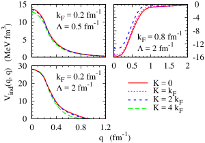
To obtain the screening correction $V_{\text{ind}}$ for finite $\bm{\mathrm{K}}$, some minor modifications of Eqs. (7) and (25) are necessary. Details are given in Appendix D. We have checked that, at least for $T=T_{c}$, the contributions to the integrals in Eqs. (39) and (40) come only from $K\lesssim 2k_{F}$. As seen in Fig. 13, numerically it turns out that the $K$ dependence of $V_{\text{ind}}$ is very weak for $K<2k_{F}$ in the range of $k_{F}$ where the NSR correction can be expected to be important. We will therefore neglect this $K$ dependence and use in Eqs. (39) and (40), the screening correction calculated for $K=0$.

There are a couple more points that need to be discussed. For instance, now one has two different densities, the uncorrelated one, $\rho_{0}$, and the corrected one, $\rho_{\text{tot}}$. The question arises which density one should use in the calculation of the induced interaction $V_{\text{ind}}$. Since $V_{\text{ind}}$ is computed with uncorrelated propagators and occupation numbers, it seems more appropriate to take only the uncorrelated density $\rho_{0}$ into account in the calculation of $V_{\text{ind}}$. From the derivation of Eqs. (39) and (40) it is also clear that the derivatives $\partial/\partial\mu$ should be taken with the interaction $V_{\text{ind}}$ kept constant (and the effective mass $m^{*}$, too). This points to fundamental problems of the present approach, which is clearly not a fully consistent treatment of both particle-particle and particle-hole fluctuations. Nevertheless, we expect to get at least a rough idea about the change of the NSR effect when the pair correlations are modified by screening.

V.2 Results

Before discussing the critical temperature as a function of density, let us look at the density correction. The un-subtracted correlated density, $\rho_{\text{corr},1}$ as a function of the Fermi-momentum corresponding to the uncorrelated density $\rho_{0}$, denoted here as $k_{F}^{0}=(3\pi^{2}\rho_{0})^{1/3}$, is shown in Fig. 14.

Figure 14: The un-subtracted correlated density $\rho_{\text{corr},\,1}$ as a function of the Fermi momentum $k_{F}^{0}$ with and without the screening correction, calculated at the respective critical temperatures $T_{c}$. Here, the black solid lines and the red dashed lines show the results for the two cutoffs of $\Lambda=2.0\,\,\text{fm}^{-1}$ and $\Lambda=2.5\,k_{F}^{0}$. The thin lines contain only $V_{0}$, while the thick lines include the induced interactions. The inset in the figure magnifies the cutoff dependence in $\rho_{\text{corr},\,1}$ at low densities. The Fermi-liquid parameters are calculated using the SLy4 interaction.

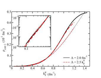
The black solid lines and the red dashed lines represent two different cutoff choices, a constant cutoff $\Lambda=2.0\,\,\text{fm}^{-1}$ and a density dependent cutoff $\Lambda=2.5\,k_{F}^{0}$. The thin lines show the correlated density $\rho_{\text{corr},1}$ with only the free-space interaction $V_{0}$. Analogous to Fig. 5 of LABEL:Ramanan2013, we see that $\rho_{\text{corr},1}$ with only $V_{0}$ is independent of the cutoff. With the inclusion of the induced interaction (thick lines) we note that the cutoff dependence of $\rho_{\text{corr},1}$ is again negligible, except at very low densities (see inset), where we found stronger screening with the variable cutoff compared to the fixed cutoff (cf. Fig. 12). In addition, up to $k_{F}^{0}\sim 0.7\,\,\text{fm}^{-1}$, the correlated density $\rho_{\text{corr},1}$ with the induced interaction is smaller than the correlated density without the induced interaction, consistent with the earlier observation that the induced interaction screens $V_{0}$. However, in the range of Fermi-momenta where the induced interaction anti-screens $V_{0}$, the correlated density $\rho_{\text{corr},1}$ is larger than the corresponding quantity without the induced interaction.

Let us now turn our attention to the correlated density with the first-order (Hartree-Fock) subtraction, $\rho_{\text{corr}}$. The dependence of $\rho_{\text{corr}}$ on $k_{F}^{0}$ is shown in Fig. 15.

Figure 15: Subtracted correlated density $\rho_{\text{corr}}$ as a function of $k_{F}^{0}$ with and without screening, calculated at the respective critical temperatures. See Fig. 14 for details.

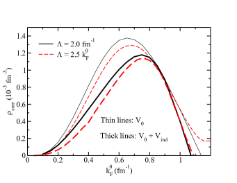
As in Fig. 14, the black solid lines and the red dashed lines show results for the two different cutoffs: the constant cutoff $\Lambda=2.0\,\,\text{fm}^{-1}$ and the density dependent cutoff $\Lambda=2.5\,k_{F}^{0}$, respectively. For low $k_{F}^{0}$, we see that the correlated density with the inclusion of the induced interaction (thick lines) is smaller than in the $V_{0}$-only case (thin lines) which is consistent with the screening of $V_{0}$ by $V_{\text{ind}}$ and similar to the trend seen in Fig. 14. However, what is surprising is that even in the region where $V_{\text{ind}}$ anti-screens $V_{0}$, the correlated density gets smaller with the inclusion of $V_{\text{ind}}$ compared to the $V_{0}$-only case. Further, one notices strong cutoff dependence in the low $k_{F}^{0}$ region if one compares the solid black line with the red dashed line, both with and without the inclusion of the induced interaction. Both these observations are completely different from Fig. 14 and are clearly the effect of the Hartree-Fock subtraction. For the density dependent cutoff, at low-densities, this subtraction should get better as the interaction gets more perturbative at smaller cutoffs. However, at high densities, where the subtraction $\rho_{\text{corr},2}$ is almost of the same magnitude as $\rho_{\text{corr},1}$ itself, the Hartree-Fock approximation is not precise enough to give a reliable result for the subtracted $\rho_{\text{corr}}$. Hence, the suppression of the correlated density for higher $k_{F}^{0}$ in Fig. 15, once the induced interaction is included, is probably unphysical. Fortunately, in this region, $\rho_{\text{corr}}$ is completely negligible compared to $\rho_{0}$.

Now we are in the position to discuss the final results for the critical temperature $T_{c}$ as a function of $k_{F}$, displayed in Fig. 16.

Figure 16: $T_{c}$ versus $k_{F}$: (Left panel) Results with fixed cutoff $\Lambda=2\,\text{fm}^{-1}$; (Right panel) density dependent cutoff $2.5\,k_{F}$. The green dashed-dotted lines are the full results including the induced interaction $V_{\text{ind}}$ and the correlated density $\rho_{\text{corr}}$ in the NSR framework. For comparison, we also show the BCS result (only $V_{0}$ and $\rho_{0}$, black solid lines) and the results obtained with the induced interaction $V_{\text{ind}}$ but without the NSR correction (red dashed lines).

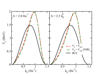
Note that in the NSR framework, $T_{c}$ as a function of $\mu$ is computed as usual, and only the relation between $\mu$ and $k_{F}$ (and $\rho$) is changed. Here, $k_{F}$ denotes the Fermi momentum corresponding to the total density including $\rho_{\text{corr}}$, i.e., $k_{F}=(3\pi^{2}\rho_{\text{tot}})^{1/3}$ (green dashed-dotted lines). As a consequence, the presence of the correlated density $\rho_{\text{corr}}$ shifts the curve slightly to the right. In order to make easy comparisons, we also show the BCS result (solid line) and the results obtained with $V_{\text{ind}}$ but without the NSR correction (red dashed lines). In both panels, we note that the pair correlations lower the transition temperature compared to the one with screening alone at the same $k_{F}$. However, the trends already observed with the medium corrections (Figs. 6 and 12), i.e., screening at low densities and anti-screening at high densities, remain unchanged, since the NSR effect is much weaker than the screening or anti-screening effect of $V_{\text{ind}}$.

Please notice that the relation $\Delta_{T=0}(k_{F})=1.76\,T_{c}$ for a given $k_{F}$, mentioned in Sec. III.3, is not valid for the NSR results.

VI Conclusions

It has been known for a long time that screening corrections have a very strong effect on the superfluid transition temperature of neutron matter. Also the fact that the RPA, diagram (b), reduces the effect of diagram (a), has been known before Cao2006 . However, in LABEL:Cao2006 the effect of diagram (b) was too weak to overcome the strong screening generated by diagram (a), while we find that, around $n\gtrsim 0.01-0.02\,\text{fm}^{-3}$, the net effect of $V_{\text{ind}}$ is attractive and screening turns into anti-screening. A similar effect was found in LABEL:Schulze1996, but only at much higher densities ($n\gtrsim 0.07\,\text{fm}^{-3}$). There are three main differences between our calculation and that of LABEL:Cao2006. First, we are using $V_{\text{low}\,k}$ while in Cao2006 the Brückner $G$ matrix was used in the vertices. Second, while we keep the full momentum dependence of the non-local interaction, the vertices in Cao2006 were replaced by an average matrix element. Probably the most important difference, however, is the choice of the Landau parameters. Here, we take them from a phenomenological energy density functional (SLy4). Since this functional was fitted to QMC results for the neutron matter equation of state, we assume that the Landau parameters are rather well determined. The anti-screening effect arises primarily from the enhancement of the attractive density ($S=0$) fluctuations due to the strongly negative $f_{0}$ parameter. In Cao2006 , on the contrary, the Landau parameters were obtained following the so-called Babu-Brown theory as explained in Schulze1996 . This results in particular in a much smaller (less negative) value of the $f_{0}$ parameter, and as a consequence, the density fluctuations are not strong enough to compensate for the repulsive effect of the spin-density ($S=1$) fluctuations.

We addressed in some detail the problem of the low density limit. When a constant (density-independent) potential $V$ is used in the vertices of diagram (a), the screening effect disappears at low density, although from the weak-coupling formula one would conclude that the gap should be reduced by the factor $(4e)^{-1/3}$ predicted by GMB Gorkov1961 . We explained why the weak-coupling formula fails in this particular case. We then observed that GMB used the full $\mathcal{T}$ matrix instead of the potential $V$ in the vertices of diagram (a). This allowed us to finally recover the GMB result, namely by using for each density a $V_{\text{low}\,k}$ interaction evolved to a cutoff $\Lambda$ that scales with $k_{F}$. In this way, one ensures that, on the one hand, one does not cut the relevant degrees of freedom ($q\lesssim k_{F}$), and on the other hand, the Born term is already a reasonable approximation to the full $\mathcal{T}$ matrix at momenta of the order of $q\sim k_{F}$.

In the last part of the paper we discussed the effect of preformed pairs on the critical temperature $T_{c}$ in the NSR framework. In spite of some cutoff and regulator dependence in the detailed study of the correlated density $\rho_{\text{corr}}$, one can clearly see that due to $\rho_{\text{corr}}$ the critical temperature $T_{c}$ for a given density is slightly reduced. But this effect is much less important than the induced interaction. Compared to ultracold atoms in the unitary limit or even on the BEC ($a>0$) side of the BCS-BEC crossover, neutron matter remains more or less in a weakly coupled regime at all densities.

There remain obviously many open questions. For instance, as discussed in Cao2006 , the reduction of the quasiparticle residue $Z<0$ can lead to a reduction of $T_{c}$, and this effect has not been included in the present study. Another point that clearly needs to be improved is the Landau approximation in the RPA. In principle, it is only valid for momentum transfer $k\ll k_{F}$, but in the induced interaction, the relevant range of momentum transfers is $0\leq k\leq 2k_{F}$. In the framework of Skyrme interactions it is actually straight-forward to solve the RPA beyond the Landau approximation, and this issue will be addressed in a future study.

Concerning the meaning of the density dependent cutoff introduced in Sec. IV.2, one might wonder how this is related to the so-called functional renormalization-group approach in which one solves flow equations in the medium, integrating out all momenta except the Fermi surface. Such approaches have been used to include screening corrections in a non-perturbative way for neutron matter Schwenk2003 and ultracold atoms Gubbels2008 ; Floerchinger2008 . In the context of the small cutoff, one should also mention that lowering the cutoff induces three- and higher-body interactions. These are neglected in $V_{\text{low}\,k}$ since it is obtained for two particles in free space. A better approach in this respect would be the in-medium similarity renormalization group Hergert2017 , which allows one to include many-body effects at least approximately into the effective two-body interaction.

Because of the extreme sensitivity of the gap and the critical temperature to the details of the effective interaction, it seems likely that large theoretical uncertainties will remain. Maybe astrophysical observations of neutron stars can help to decide which theory is correct.

Appendix A Partial wave expansion of the Gogny force

We expand the Gogny force as given in Ref. Decharge1980 into partial waves, neglecting the spin-orbit term as in Shen2005 . The resulting matrix elements in the $nn$ channel read:

$$\langle Q|V_{ls}|Q^{\prime}\rangle=\frac{1}{4\pi}\sum_{i=1,2}[W_{i}-H_{i}+(-1)^{S}(M_{i}-B_{i})]\\ \times(\sqrt{\pi}\mu_{i})^{3}e^{-(Q^{2}+Q^{\prime\,2})\mu_{i}^{2}/4}i_{l}(QQ^{\prime}\mu_{i}^{2}/2)$$ (41)

where $i_{l}(z)=\sqrt{\pi/2z}I_{l+1/2}(z)$ is a modified spherical Bessel function of the first kind AbramowitzStegun : $i_{0}(z)=\sinh(z)/z$, etc. The antisymmetrized matrix elements are then obtained by $\langle Q|\tilde{V}_{ls}|Q^{\prime}\rangle=[1+(-1)^{l+s}]\langle Q|V_{ls}|Q^{\prime}\rangle$. The density dependent contact term of the Gogny force does not contribute since it acts only in the neutron-proton channel.

Concerning the values of $\mu_{i}$, $W_{i}$, $H_{i}$, $B_{i}$, and $M_{i}$, we use either the parameterization D1 Decharge1980 to compare with Ref. Shen2005 or the more recent parameterization D1N Chappert2008 .

Appendix B Fermi-liquid parameters

In this work, we use the Fermi-liquid parameters from the SLy4 parameterization of the Skyrme functional Chabanat1997 or from the D1N parametrization of the Gogny force Chappert2008 . The explicit expressions in terms of the Skyrme-force parameters $t_{i}$, $x_{i}$ ($i=0\dots 3$), and $\sigma$ read Margueron2002

$$\frac{1}{m^{*}}= \frac{1}{m}+\tfrac{1}{4}[t_{1}(1-x_{1})+3t_{2}(1+x_{2})]\rho\,,$$ (42)

$$f_{0}= \tfrac{1}{2}t_{0}(1-x_{0})+\tfrac{1}{4}[t_{1}(1-x_{1})+3t_{2}(1+x_{2})]k_{F}^{2}$$

$$+\tfrac{1}{24}t_{3}(1-x_{3})(1+\sigma)(2+\sigma)\rho^{\sigma}\,,$$ (43)

$$g_{0}= \tfrac{1}{2}t_{0}(x_{0}-1)+\tfrac{1}{4}[t_{1}(x_{1}-1)+t_{2}(1+x_{2})]k_{F}^{2}$$

$$+\tfrac{1}{12}t_{3}(x_{3}-1)\rho^{\sigma}\,.$$ (44)

In the case of the Gogny force, one obtains the following expressions for the Fermi-liquid parameters Shen2005 :

$$\frac{1}{m^{*}}= \frac{1}{m}+\frac{m}{\sqrt{\pi}k_{F}}\sum_{i=1,2}\mu_{i}(W_{i}+2B_{i}-H_{i}-2M_{i})$$

$$\times z_{i}e^{-z_{i}}i_{1}(z_{i})\,,$$ (45)

$$f_{0}= \sum_{i=1,2}\frac{(\sqrt{\pi}\mu_{i})^{3}}{2}[(2W_{i}+B_{i}-2H_{i}-M_{i})$$

$$-(W_{i}+2B_{i}-H_{i}-2M_{i})e^{-z_{i}}i_{0}(z_{i})]\,,$$ (46)

$$g_{0}= \sum_{i=1,2}\frac{(\sqrt{\pi}\mu_{i})^{3}}{2}[(B_{i}-M_{i})-(W_{i}-H_{i})e^{-z_{i}}i_{0}(z_{i})]\,,$$ (47)

where $z_{i}=k_{F}^{2}\mu_{i}^{2}/2$.

Appendix C Angle-averaged Lindhard function

For $q,q^{\prime}\neq 0$, the general explicit expression for the angle-averaged Lindhard function defined in Eq. (29) reads

$$\langle\tilde{\Pi}_{0}\rangle=-\frac{1}{3}+\frac{k_{F}^{2}}{48qq^{\prime}}[F(2-x_{-})+F(2+x_{-})\\ -F(2-x_{+})-F(2+x_{+})]\,,$$ (48)

with $F(x)=x^{2}(6-x)\ln|x|$ and $x_{\pm}=|q\pm q^{\prime}|/k_{F}$. In the special case of interest $q=q^{\prime}=k_{F}$ mentioned in the main text this gives $\langle\tilde{\Pi}_{0}\rangle=-\tfrac{1}{3}\ln 4e\approx-0.795$. The expression for the cases $q\neq q^{\prime}=0$ or $q^{\prime}\neq q=0$ reads

$$\langle\tilde{\Pi}_{0}\rangle=\frac{x^{2}-4}{8x}\operatorname{artanh}\Big{(}\frac{x}{2}\Big{)}-\frac{1}{2}\,,$$ (49)

with $x=q/k_{F}$ or $q^{\prime}/k_{F}$, respectively. In the special case $q=q^{\prime}=0$, one obtains $\langle\tilde{\Pi}_{0}\rangle=-1$. For $q\gg k_{F}$ or $q^{\prime}\gg k_{F}$, $\langle\tilde{\Pi}_{0}\rangle$ tends to zero.

Appendix D Computation of the screening corrections for pairs with finite total momentum

In Fig. 1 and the corresponding Eqs. (7) and (25), we have considered from the beginning a pair at rest (with respect to the medium). However, for the NSR correction, one needs pairs with finite total momentum $\bm{\mathrm{K}}$. In order to compute the screening corrections $V_{\text{ind}}=V_{a}+V_{b}$ for $\bm{\mathrm{K}}\neq 0$, one has to change the definitions of the vectors $\bm{\mathrm{Q}}_{1}$, $\bm{\mathrm{Q}}_{1}^{\prime}$, $\bm{\mathrm{Q}}_{2}$, and $\bm{\mathrm{Q}}_{2}^{\prime}$ that appear in Eqs. (7) and (25). For diagram (a), one has to replace Eq. (9) by

$$\begin{split}&\bm{\mathrm{Q}}_{1}=\frac{\bm{\mathrm{q}}+\bm{\mathrm{p}}}{2}-\frac{\bm{\mathrm{K}}}{4}\,,\quad\bm{\mathrm{Q}}^{\prime}_{1}=\frac{\bm{\mathrm{q}}^{\prime}-\bm{\mathrm{k}}+\bm{\mathrm{p}}}{2}-\frac{\bm{\mathrm{K}}}{4}\,,\\ &\bm{\mathrm{Q}}_{2}=\frac{\bm{\mathrm{q}}+\bm{\mathrm{k}}-\bm{\mathrm{p}}}{2}+\frac{\bm{\mathrm{K}}}{4}\,,\quad\bm{\mathrm{Q}}^{\prime}_{2}=\frac{\bm{\mathrm{q}}^{\prime}-\bm{\mathrm{p}}}{2}+\frac{\bm{\mathrm{K}}}{4}\,.\end{split}$$ (50)

For diagram (b), the definition (26) has to be replaced by

$$\begin{split}&\bm{\mathrm{Q}}_{1}=\frac{\bm{\mathrm{q}}+\bm{\mathrm{p}}_{1}}{2}-\frac{\bm{\mathrm{K}}}{4}\,,\quad\bm{\mathrm{Q}}^{\prime}_{1}=\frac{\bm{\mathrm{q}}^{\prime}-\bm{\mathrm{k}}+\bm{\mathrm{p}}_{1}}{2}-\frac{\bm{\mathrm{K}}}{4}\,,\\ &\bm{\mathrm{Q}}_{2}=\frac{\bm{\mathrm{q}}+\bm{\mathrm{k}}-\bm{\mathrm{p}}_{2}}{2}+\frac{\bm{\mathrm{K}}}{4}\,,\quad\bm{\mathrm{Q}}^{\prime}_{2}=\frac{\bm{\mathrm{q}}^{\prime}-\bm{\mathrm{p}}_{2}}{2}+\frac{\bm{\mathrm{K}}}{4}\,.\end{split}$$ (51)

However, for diagram (b), this is not sufficient, because we used the isotropy to replace the sum over the three spin projections $m_{S}=-1,0,1$ of the $S=1$ particle-hole excitation by the contribution of $m_{S}=0$, multiplied by three. But for $\bm{\mathrm{K}}\neq 0$, the isotropy is lost and therefore the contributions of the three spin projections will not be equal any more. Nevertheless, after summation over $m_{S}$, the final result for $V_{b}$ can only depend on $K=|\bm{\mathrm{K}}|$ and not on the direction of $\bm{\mathrm{K}}$. Hence, we can average over the angle of $\bm{\mathrm{K}}$. By doing so, we have restored the isotropy and it is therefore again sufficient to compute only the contribution of $m_{S}=0$ and to multiply the result by three.

References

- (1) N. Chamel and P. Haensel, Living Rev. Relativity, 11, 10 (2008).
- (2) P. W. Anderson and N. Itoh, Nature 256, 25 (1975).
- (3) D. Pines and M. A. Alpar, Nature 316, 27 (1985).
- (4) B. Haskell and A. Sedrakian, arXiv:1709.10340 [astro-ph.HE].
- (5) D. G. Yakovlev and C. J. Pethick, Ann. Rev. Astron. Astrophys. 42, 169 (2004).
- (6) M. Fortin, F. Grill, J. Margueron, D. Page, and N. Sandulescu, Phys. Rev. C 82, 065804 (2010).
- (7) D. Page, J. M. Lattimer, M. Prakash and A. W. Steiner, Astrophys. J. 707, 1131 (2009).
- (8) A. Gezerlis, C. J. Pethick and A. Schwenk, in: K. H. Bennemann and J. B. Ketterson (eds.), Novel Superfluids, Volume 2 (Oxford University Press, 2014)
- (9) A. B. Migdal, Zh. Eksp. Teor. Fiz. 37 249 (1959) [Sov. Phys. JETP 10, 176 (1960)]; Nucl. Phys. 13, 655 (1959).
- (10) V. L. Ginzburg and D. A. Kirzhnits, Zh. Eksp. Teor. Fiz. 47, 2006 (1964) [Sov. Phys. JETP 20, 1346 (1965)].
- (11) V. L. Ginzburg, Usp. Fiz. Nauk 97, 601 (1969) [Sov. Phys.-Uspekhi 12, 241 (1969)]; J. Stat. Phys. 1, 3 (1969).
- (12) G. Baym, C. J. Pethick, D. Pines, and Malvin Ruderman, Nature 224, 872 (1969).
- (13) A. Sedrakian and J. W. Clark, arXiv:1802.00017 [nucl-th].
- (14) D. J. Dean and M. Hjorth-Jensen, Rev. Mod. Phys. 75, 607 (2003).
- (15) S. Srinivas and S. Ramanan, Phys. Rev. C 94, 064303 (2016).
- (16) C. Drischler, T. Krüger, K. Hebeler and A. Schwenk, Phys. Rev. C 95, 024302 (2017).
- (17) P. Papakonstantinou and J. W. Clark, J. Low. Temp. Phys. 189, 361 (2017).
- (18) A. Rios, A. Polls and W. H. Dickhoff, J. Low. Temp. Phys. 189, 234 (2017).
- (19) A. Rios, D. Ding, H. Dussan, W. H. Dickhoff, S. J. Witte and A. Polls, J. Phys. Conf. Ser. 940, 012014 (2018).
- (20) J. Wambach, T. L. Ainsworth and D. Pines, Nucl. Phys. A 555, 128 (1993).
- (21) H. J. Schulze, J. Cugnon, A. Lejeune, M. Baldo and U. Lombardo, Phys. Lett. B 375, 1 (1996).
- (22) C. Shen, U. Lombardo and P. Schuck, Phys. Rev. C 67, 061302 (2003).
- (23) Caiwan Shen, U. Lombardo, and P. Schuck, Phys. Rev. C 71, 054301 (2005).
- (24) L. G. Cao, U. Lombardo, and P. Schuck, Phys. Rev. C 74, 064301 (2006).
- (25) A. L. Fetter and J. D. Walecka, Quantum Theory of Many-Particle Systems (McGraw-Hill, New York, 1971).
- (26) K. Hebeler and A. Schwenk, Phys. Rev. C 82, 014314 (2010).
- (27) S. Babu and G. E. Brown, Ann. Phys. (NY) 78, 1 (1973).
- (28) S. Gandolfi, A. Yu. Illarionov, S. Fantoni, F. Pederiva, and K. E. Schmidt, Phys. Rev. Lett. 101, 132501, (2008).
- (29) T. Abe and R. Seki Phys. Rev. C 79, 054003 (2009).
- (30) A. Gezerlis and J. Carlson, Phys. Rev. C 81, 025803 (2010).
- (31) P. Nozières and S. Schmitt-Rink, J. Low. Temp. Phys. 59, 195 (1985).
- (32) M. Jin, M. Urban, and P. Schuck, Phys. Rev. C 82, 024911 (2010).
- (33) G. C. Strinati, P. Pieri, G. Röpke, P. Schuck, and M. Urban, Phys. Rep. 738, 1 (2018).
- (34) M. Matsuo, Phys. Rev. C 73, 044309 (2006).
- (35) J. Margueron, H. Sagawa, and K. Hagino, Phys. Rev. C 76, 064316 (2007).
- (36) B. Y. Sun, H. Toki, and J. Meng, Phys. Lett. B 683, 134 (2010).
- (37) S. Ramanan and M. Urban, Phys. Rev. C 88, 054315 (2013)
- (38) J. W. Negele and D. Vautherin, Nucl. Phys. A 207, 298 (1973).
- (39) M. Baldo, E. E. Saperstein, and S. V. Tolokonnikov, Phys. Rev. C 76, 025803 (2007).
- (40) C. A. R. Sá de Melo, M. Randeria, and J. R. Engelbrecht, Phys. Rev. Lett. 71, 3202 (1993).
- (41) L. Pisani, A. Perali, P. Pieri, and G. C. Strinati, Phys. Rev. B 97, 014528 (2018).
- (42) L. P. Gor’kov and T.K. Melik-Barkhudarov, Zh. Eksp. Teor. Fiz. 40, 1452 (1961) [Sov. Phys. JETP 13, 1018 (1961)].
- (43) See ancillary files of the present arxiv submission for data files containing matrix elements with and without induced interaction.
- (44) J. Kuckei, F. Montani, H. Müther, and A. Sedrakian, Nucl. Phys. A 723, 32 (2003).
- (45) D. A. Varshalovich, A. N. Moskalev, V. K. Khersonskii, Quantum Theory of Angular Momentum (World Scientific, Singapore, 1988).
- (46) S. K. Bogner, R. J. Furnstahl, S. Ramanan, and A. Schwenk, Nucl. Phys. A 784, 79 (2007).
- (47) J. Dechargé and D. Gogny, Phys. Rev. C 21, 1568 (1980).
- (48) F. Chappert, M. Girod, and S. Hilaire, Phys. Lett. B 668, 420 (2008).
- (49) A. Sedrakian, T. T. S. Kuo, H. Müther, and P. Schuck, Phys. Lett. B 576, 68 (2003).
- (50) E. Chabanat, P. Bonche, P. Haensel, J. Meyer, and R. Schaeffer, Nucl. Phys. A 627, 710 (1997).
- (51) H. Heiselberg, C. J. Pethick, H. Smith, and L. Viverit, Phys. Rev. Lett. 85, 2418 (2000).
- (52) J. W. Clark, in R. A. Broglia and V. Zelevinsky (eds.), Fifty Years of Nuclear BCS (World Scientific, Singapore 2013), 360.
- (53) S. K. Bogner, A. Schwenk, R. J. Furnstahl and A. Nogga, Nucl. Phys. A 763, 59 (2005).
- (54) S. K. Bogner, R. J. Furnstahl, S. Ramanan and A. Schwenk, Nucl. Phys. A 773, 203 (2006).
- (55) K. Hebeler, A. Schwenk and B. Friman, Phys. Lett. B 648, 176 (2007).
- (56) R. Zimmermann and H. Stolz, Phys. Status Solidi B 131, 151 (1985).
- (57) A. Schwenk, B. Friman and G. E. Brown, Nucl. Phys. A 713, 191 (2003).
- (58) K. B. Gubbels and H. T. C. Stoof, Phys. Rev. Lett. 100, 140407 (2008).
- (59) S. Floerchinger, M. Scherer, S. Diehl, and C. Wetterich, Phys. Rev. B 78, 174528 (2008).
- (60) H. Hergert, S. K. Bogner, J. G. Lietz, T. D. Morris, S. J. Novario, N. M. Parzuchowski, and F. Yuan, Lect. Notes Phys. 936, 477 (2017).
- (61) M. Abramowitz and I. A. Stegun (eds.), Handbook of Mathematical Functions (Dover, New York 1965).
- (62) J. Margueron, J. Navarro, and Nguyen Van Giai, Phys. Rev. C 66, 014303 (2002).