Paramotopy: Parameter homotopies in parallel
Abstract
Numerical algebraic geometry provides a number of efficient tools for approximating the solutions of polynomial systems. One such tool is the parameter homotopy, which can be an extremely efficient method to solve numerous polynomial systems that differ only in coefficients, not monomials. This technique is frequently used for solving a parameterized family of polynomial systems at multiple parameter values. Parameter homotopies have recently been useful in several areas of application and have been implemented in at least two software packages. This article describes Paramotopy, a new, parallel, optimized implementation of this technique, making use of the Bertini software package. The novel features of this implementation, not available elsewhere, include allowing for the simultaneous solutions of arbitrary polynomial systems in a parameterized family on an automatically generated (or manually provided) mesh in the parameter space of coefficients, front ends and back ends that are easily specialized to particular classes of problems, and adaptive techniques for solving polynomial systems near singular points in the parameter space. This last feature automates and simplifies a task that is important but often misunderstood by non-experts.
1 Introduction
The methods of numerical algebraic geometry provide a means for approximating the solutions of a system of polynomials , i.e., those points (perhaps forming positive-dimensional components–curves, surfaces, etc.) such that . There are many variations on these methods, but the key point is that polynomial systems of moderate size can be solved efficiently via homotopy continuation-based methods. In the case of a parameterized family of polynomial systems , where the coefficients are polynomial in the parameters , a particularly efficient technique comes into play: the parameter homotopy [28]111In fact, this technique applies when the coefficients are holomorphic functions of the parameters [28], but we restrict to the case of polynomials as Bertini is restricted to polynomials..
Parameter homotopies are quite powerful for many classes of problems that arise in practice; before detailing the theory of parameter homotopies, we first describe the basics of using standard, non-parameter homotopies. The process of using a standard homotopy to solve a system begins with the construction of a polynomial system that is easily solved. Once the system is solved, the solutions of are tracked numerically by predictor-corrector methods as the polynomials of are transformed into those of . Thanks to the underlying geometry, discussed for example in [27] or [4], we are guaranteed to find a superset of the set of isolated solutions of . The set is easily trimmed down to in a post-processing step [6].
One of the two extremes among the many choices of homotopy constructions is the total degree homotopy, which typically requires the tracking of many more paths than the number of solutions of . At the other extreme, polyhedral homotopies require the tracking of the exact number of paths as the number of solutions of , under the assumption that the coefficients of are generic, but even for systems of moderate size, this reduction in the number of paths comes at the cost of significant computational effort to solve . Many possible homotopies exist between these two, each with varying levels of complexity for solving and varying numbers of paths to be tracked.
Parameter homotopies behave nicely, as the number of paths to be followed is exactly equal to the number of isolated solutions of for almost all values of (under the common assumption that has positive volume in its ambient Euclidean space) and the solution of a single will work for almost all values of , so only one round of precomputation is needed regardless of the number of polynomial systems to be solved. This is described in more detail in §2.
Parameter homotopies are not new and have been used in several areas of application [8, 17, 25, 26] and implemented in at least two software packages for solving polynomial systems: Bertini [5] and PHCpack [29]. These implementations allow the user to run a single parameter homotopy from one parameter value with known solutions to the desired parameter value, , with the solutions at provided by the user.
The new software package that is the focus of this article differs from these other two implementations in the following ways:
-
1.
Paramotopy accepts as input the general form of the parameterized family ( given as indeterminates), chooses a random , and solves via a Bertini run222Bertini provides this functionality as well.;
-
2.
Paramotopy builds a mesh in the parameter space given simple instructions from the user (or uses a user-provided set of parameter values) and performs parameter homotopy runs from to each other in the mesh;
-
3.
Paramotopy carries out all of these runs in parallel, as available333Bertini and PHCpack both have parallel versions, but not for multiple parameter homotopy runs.;
-
4.
Paramotopy includes adaptive schemes to automatically attempt to find the solutions of from starting points other than , if ill-conditioning causes path failure in the initial attempt; and
-
5.
Paramotopy is designed to simplify the creation of front ends and back ends specialized for particular applications.
The purpose of this article is two-fold: to provide a refresher on parameter homotopies and to describe the software package Paramotopy. Parameter homotopies are described in more technical detail in the next section, followed by implementation details of Paramotopy in §3. Finally, a few examples and timings are provided in §4.
2 Homotopies
In this section, we introduce homotopy continuation (§2.1), then the special setting of parameter homotopies (§2.2).
2.1 Homotopy continuation
Given a polynomial system to be solved, standard homotopy continuation consists of three basic steps:
-
1.
Choose a start system similar in some way to that is “easy” to solve;
-
2.
Find the solutions of and form the new homotopy function given by , where is randomly chosen; and
- 3.
There are many variations on this general theme, but we focus here on the basic ideas, leaving details and alternatives to the references.
Remark 2.1.
- 1.
- 2.
-
3.
Notice that has the property that and .
-
4.
The extra included in homotopy function introduces randomness to the paths to be followed. This “gamma trick” is discussed later in this section and is central to the probability one nature of homotopy continuation methods.
As a simple example of the choice of , let’s consider the total degree homotopy. Let denote the degrees of the polynomials of . One instance of a total degree or Bézout homotopy is
with . This system has trivially-computed solutions, so a homotopy using this as a start system would have that number of paths, regardless of the number of solutions of . A generalization of this sort of start system, the multihomogeneous or -hom start system, is the standard in Bertini [5] and is thus the main type of start system used in our implementation; see [27, 4] for more on that particular choice. Regeneration [15] is a recent advance that will also greatly increase the efficiency of non-parameter homotopy runs.
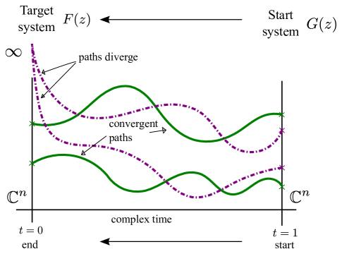
Once is solved and is formed, the solutions of for varying values of may be visualized as curves. Indeed, as varies continuously, the solutions of will vary continuously, so each solution sweeps out a curve or path (also sometimes called a solution curve or solution path) as moves from 1 to 0. A schematic of four such paths is given in Figure 1.
Predictor-corrector methods are used to follow the solutions of to those of along these paths. For example, an Euler (tangent) predictor will find a point near a solution of for some given , after which Newton’s method may be used to correct back to the solution at . This process is repeated to move forward along the path, towards . This is a vast oversimplification of what we refer to as standard homotopy methods (as opposed to parameter homotopies); indeed, in Bertini, Euler’s method has been replaced with more accurate predictors [1], potential path-crossings are handled with adaptive multiprecision path tracking techniques [7, 3], powerful numerical techniques called endgames are employed near the end of the path () [23, 24, 2], and, for large problems, all of this is done in parallel [4].
Despite all the modern safeguards against numerical difficulties, problems can still arise. If a path is not successfully tracked from all the way to a solution at , we refer to this as a path failure. Causes for path failures in Paramotopy are inherited directly from those of Bertini [4], as Paramotopy relies on Bertini for all path tracking. There are numerous such causes, though one of the most common comes from the situation of having two paths come near one another. In that case, the Jacobian matrix of the homotopy function becomes ill-conditioned, causing an increase in precision and/or reductions to the step size. Precision has a maximum allowed value within Paramotopy and Bertini, while the step size has a minimum allowed value. If either of these thresholds is broken, the path is declared a failure. It is important to note that path failures are not failures of the methods or the software. On the contrary, a path failure is a signal to the user that the geometry of the path is somehow particularly tricky and that more care needs to be taken. The mitigation of common path failures for parameter homotopies is described in §3.2.
2.2 Parameter homotopies
Suppose we wish to solve a parameterized polynomial system in variables and parameters at a (possibly very large) number of points in parameter space, i.e., we want to find such that for varying values . If we know all isolated, finite, complex solutions at some generic point in a convex444Handling non-convex parameter spaces is significantly more difficult and is described later. parameter space , the underlying theory allows us to make use of a parameter or coefficient-parameter homotopy [28]. The usefulness of this software becomes readily apparent from the following proposition, proved in somewhat different language in [27]. The proposition guarantees that we can find the isolated, finite, complex solutions of simply by following paths through the parameter space, , from the solutions of .
Proposition 2.2.
The number of finite, isolated solutions of is the same for all except for a measure zero, algebraic subset of .
This proposition gives us a probability one guarantee that a randomly chosen path through parameter space will avoid . Furthermore, assuming is convex, a straight line segment through parameter space from a randomly chosen to a prespecified target will, with probability one, not pass through the set . By moving in a straight line from a random starting point in parameter space, we should not have any path-crossings or divergent paths, i.e., the straight line from our starting point to should miss .
This immediately implies a (known) technique for solving many polynomial systems from the same parameterized family with parameter space . First, find all finite, isolated, complex solutions for some randomly chosen . We refer to this as Step 1. Second, for each parameter value of interest, , simply follow the finite, isolated, complex solutions through the simple homotopy . We refer to this as Step 2. Notice that the randomly chosen from standard homotopies can be neglected in this homotopy since is chosen randomly. We describe in §3.2 how we monitor these Step 2 runs in case paths fail and also how we handle such failures.
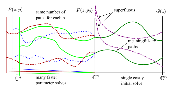
For the cost of a single Step 1 solve at some random point in the parameter space, we may rapidly solve many other polynomial systems in the same parameterized family. Indeed, there are a minimal number of paths to follow in each Step 2 run and no pre-computation cost exists beyond the initial solve at .
The randomness of
It is important to choose a random complex in . The measure zero set described above contains all parameter values for which the number of solutions is less than the generic number of solutions. If we were to choose from , we would not find all solutions for the parameter values of interest since we would not have as many paths as the number of solutions at each parameter value of interest. By choosing at random, there is a zero probability that . If we were to use a special , there is no guarantee that .
The value of parameter homotopies
To get a sense of the savings from using parameter homotopies over repeated standard homotopies, suppose you can solve a parameterized polynomial system for a single point in parameter space with paths. Suppose further that you wish to solve for different points in parameter space, each generically having solutions. With the repeated use of a standard homotopy, you would need to follow a total of paths. With a single Step 1 run at a randomly chosen complex point in the parameter space, followed by Step 2 runs to the points of interest, you would need to follow a total of paths. The savings are clearly significant if , especially when is large. For example, if , , but (these are not exaggerated numbers), the number of paths to be tracked is reduced from 10 million to 20 thousand by using parameter homotopies, but there is no degradation in the value of the output. If , it is unclear whether there is value in using a parameter homotopy. Indeed, it has been noticed that paths behave differently for different types of homotopies. This is an interesting open problem but is beyond the scope of this paper.
Handling non-convex parameter spaces
The above restriction that be convex simplifies the discussion but is not theoretically necessary. In our experience, it seems that most parameter spaces are convex, though it sometimes happens that parameter spaces may not be convex and it could very well be that, for certain application areas, parameter spaces are typically non-convex, perhaps not even path-connected.
If is not convex, it can happen that a line segment from to passes out of . In that case, it could happen that the root count in the ambient Euclidean space containing is higher than that of , resulting in the failure of paths when passing from back into .
One potential mitigation is to replace with , accepting that there will be more paths to follow from a generic . In this case, care must be taken that paths remain within once they first enter , since the first entry into could cause path failures, leading us back to the situation of the previous paragraph. Another mitigation for non-convex parameter spaces is to force the path to stay within , either by parameterizing some curve from to or by choosing a piecewise linear path that stays within (if one exists). See nested parameter spaces in [4] for more on this situation.
In any case, it is important to note that
-
1.
Paramotopy makes the assumption that the parameter space is convex, but
-
2.
With care, users can handle other sorts of parameter spaces (including non-convex parameter spaces) via Paramotopy.
In the next section, we describe the main algorithm for Paramotopy, involving one Step 1 run, followed by many Step 2 runs. We also point out some of the more technical aspects of Paramotopy, such as the use of parallelization and data management, as well as the use of multiple parameter homotopy runs from different starting points to find the solutions for particular parameter values for which there were path failures in the initial parameter homotopy.
3 Implementation details
Paramotopy is a C++ implementation of parameter homotopies, relying heavily on Bertini [5]. In this section, we provide the main mathematical algorithm, Algorithm 1, pseudocode for the fundamental algorithm, discuss how path failures are managed automatically, provide the technical details on both parallelization and data management in Paramotopy, and provide details on how to interface with Paramotopy from Matlab.
3.1 Main algorithm
We first present the main parameter homotopy algorithm that is implemented in Paramotopy. Note in particular the input value and the while loop at the end, both included to help manage path failures during the Step 2 runs. Also, note that this algorithm assumes that , for some . The use of Paramotopy for other parameter spaces is described in §3.3.
Remark 3.1.
To find all solutions for all , we must have that all solutions of are nonsingular as we can only follow paths starting from nonsingular solutions during the parameter homotopies after the first run. Deflation [20, 16] could be used to regularize singularities in Step 1 before beginning Step 2, but this is not currently implemented.
Remark 3.2.
Paramotopy does not currently check the quality of the Step 1 results. While theory dictates that some paths converge while others diverge as , the reality is that paths can fail for numerical reasons. For example, the path tracker can jump between paths if two paths come very near. This is largely mitigated in Bertini via adaptive precision and a check at (with as the default in Bertini) whether all paths are still distinct. But there is no known way to remove such crossings with certainty. Thus, the user should consider reviewing the output of Step 1 before launching Step 2. If nothing else, a rerun of Step 1 could increase confidence in the results.
3.2 Handling path failures during Step 2
If a path fails during a Step 2 run for some parameter value , Paramotopy will automatically attempt to find the solutions at by tracking from a different randomly chosen parameter value . It will repeat this process times, with specified by the user. This is the content of the while loop at the end of the Main Algorithm.
The idea behind this is that paths often fail for one of two reasons:
-
1.
the path seems to be diverging, or
-
2.
the Jacobian matrix becomes so ill-conditioned that either the steplength drops below the minimum allowed or the precision needed rises above the maximum allowed.
For parameter homotopies, a path failure of the first type is possible for either of two reasons: either
the path really is diverging or the norm of the solution is above a particular threshold.
In the former case, it can happen that the nature of the solution set at target value differs from that at
a generic point in the parameter space, e.g., there could be fewer finite solutions at .
Such path failures are captured and reported by Paramotopy, but there is simply no hope for
“fixing” them as this result is a natural consequence of the geometry of the solution set, i.e.,
is inherently different from other points in parameter space, so Paramotopy takes the
correct action in reporting it. In the latter case, it can happen that the scaling of
the problem results in solutions that are large in some norm, e.g., as is the default in the current
version of Bertini. If this is suspected, the user could rescale the system or adjust the threshold
MaxNorm and run the problem again.
For the second type of path failure, the ill-conditioning is caused by the presence of a singularity near or on the path between and . By choosing new starting point “adequately far” from , it should be feasible to avoid the ill-conditioned zone around unless is near the target value . In this last case, it is unlikely that choosing different starting points will have any value, which is why we have capped the number of new starting points allowed at .
For now, the new point is chosen randomly in the unit hypercube. Future work will detect where in parameter space the failures have occurred and bound away from this region.
Since it cannot easily be determined which paths from to correspond to the failed paths from to , there is no choice but to follow all paths from to . To find all solutions at , we simply use a parameter homotopy to move the solutions at to those at . Of course, if there are path failures, we must choose yet another and try again.
3.3 Handling parameter spaces other than
As described near the end of §2.2, Paramotopy may be used to handle parameter spaces other than the simplest parameter space, for some . However, some changes are needed in the algorithm.
If is a proper, convex subset of , Algorithm 1 needs only one change: must be somehow chosen within . To accommodate this, Paramotopy allows the user to specify .
If is a proper, non-convex set, more work is required. The Step 1 run would be the responsibility of the user, as in the previous paragraph, and it would be up to the user to string together subsequent Paramotopy runs to stay within . As this case appears to be both uncommon and highly complicated, we leave handling such situations the responsibility of the user.
3.4 Parallelization and data management
One of the features of Paramotopy that sets it apart from Bertini is the use of parallel computing for multiple parameter homotopies. Bertini includes parallel capabilities for a single homotopy run, but not for a sequence of runs. Parallelization was achieved using the head-worker paradigm, implemented with MPI. A single process controls the distribution of parameter points to the workers, which constitute the remainder of the processes. Workers are responsible for writing the necessary files for Bertini and for writing their own data to disk.
Bertini creates structures in memory by parsing an input file. As input is interpreted, several other files are created. These contain the straight line program, coefficient values, variable names, etc. Since the monomial structure of the polynomials in each Step 2 run is the same, almost all of these files are identical from one run to the next, so almost all this parsing is unnecessary. The only file that needs to be changed between runs is the file containing parameter values. Parsing requires a significant amount of time especially when compared to the short time needed for parameter homotopy runs, and since we call Bertini repeatedly, we eliminate as much of this parsing as possible. We do so by calling certain Bertini functions from a compiled library, so as to prevent both the repeated parsing of an input file and to preserve the necessary structure of the temporary files.
As Bertini runs through the paths of a homotopy, it records path-tracking data files. To prevent proliferation in the number of files needed to contain the data from the Paramotopy run, the Bertini output data is read back into memory, and dumped into a collective data file. The collective data files have a maximum buffer size (the default of which is 64MB), and once the buffer size is reached, the data in the buffer is written to the file, and the process repeats by storing the Bertini output data in memory until the buffer is full once more. On modern systems, in principle all data could be collected into a single file, but transfer of data out of a computing cluster can be cumbersome with extremely large files.
Repeated writing and reading is taxing on hard drives and clogs a LAN if the workers are using network drives. To free workers from having to physically write temporary files to electronic media storage, an option is provided to the user to exploit a shared memory location (or ramdisk), should it be available. The default location for this is /dev/shm. This is commonly available on Linux installations such as CentOS.
As a piece of scientific software, knowledge of efficiency and performance are important. To this end, we have developed a custom class for timing statements that records information for each parameter point by utilizing the chrono standard library. This enables analysis of performance by process type, which appears below in the demonstration sections (4). If the user is not interested in timing, the program may be compiled without the timing statements by making use of the appropriate compiler flags.
3.5 Front ends and back ends
Real-world problems may involve many parameters. This could be problematic when one wants to discretize a parameter space into a uniform sample as the number of parameter points of interest can easily reach into the millions or even billions. Hence, Paramotopy contains support for both linear uniform meshes of parameters, as well as user-defined sets of parameter values stored in a text file. Systems with few parameters can make excellent use of computer-generated discretizations. In contrast, systems with many parameters perhaps could use the Monte Carlo sampling method to collect useful information. To use this functionality, the user must generate a text file containing whitespace-separated real and imaginary pairs for each parameter, with distinct parameter points being on separate lines. An example with a user-defined parameter sampling is given in Section 4.1, while computer generated regular meshes are used in Sections 4.2-4.4.
A generic Matlab interface for gathering, saving, and plotting data from an arbitrary Paramotopy run is provided on the Paramotopy website. It can handle both the mesh-style parameter discretizations, as well as user-defined sets. The mesh-style runs generate an -dimensional array, with the number of solutions, number of real solutions, and solution values stored accordingly. Because the user-defined runs may not emit such a convenient method of storage, a 1D array is created, with line number from the parameter file corresponding to the index in the Matlab data structure.
Regarding plotting in this Matlab function, two and three dimensional data sets are plotted automatically. Higher dimension data can be plotted with the user’s choice of variables appearing on the axes, with a variable used for coloring the points if desired, for display of up to 4 dimensions. Additional basic display techniques included are movie-making and display of the number of real solutions in parameter space. Details on how to use these features may be found in the Paramotopy user’s manual, available from the Paramotopy website.
Other software packages, including surfex and surfer, can be used for viewing algebraic surfaces given by one polynomial in three variables [18, 14]. Bertini_real is another such software package that has no such restrictions on the number of polynomials and variables, though it will find only the real solutions within complex curves and surfaces [9].
4 Examples
In this section, we walk through a few examples of Paramotopy runs demonstrating various features.
4.1 Kinematics
Kinematics problems can often be cast in polynomial systems language; see e.g. [19, 8] and a slew of others. Robotic arms, whether prismatic or revolute in nature, can be described in terms of now-canonical parameters [10]. Using homogeneous matrices, inverse kinematic equations can be derived for any robot, and in the case of revolute joints, are expressed in terms of sines and cosines of the joint variables. Finally, by coupling such pairs through a Pythagorean identity, the trigonometric functions can be made polynomial.
Here, we present a very basic manipulator, purely for demonstration purposes. Consider a three-link spatial manipulator, with each link having joint length unity. For such a robot, Denavit Hartenberg (DH) parameters are given in Table 1. To get a basic mapping of the workspace, we can sample coordinates randomly, and feed Paramotopy this sample. See Input 1. Running Paramotopy will then give us a map of the space, in terms of the number of real configurations possible for each point in space, as well as allowing us to estimate the volume of the workspace.
| (m) | (m) | ||
|---|---|---|---|
| 1 | 0 | ||
| 0 | 1 | 0 | |
| 1 | 0 |
A plot of a random point sampling with coloring according to the number of real solutions is given in Figure 3. Every point in the sample has an even number of real solutions, with a core around the origin having four, and the remainder having two. A total of 58% of samples had a positive number of real solutions; therefore, we can estimate that the volume of the workspace for this robot is cubic units.
The ability to handle arbitrary parameter samples makes Paramotopy a powerful tool. One can perform initial sampling of a space, interpret the results using the Matlab codes provided, and make a new run using a refined sample. Alternatively, one can perform non-linear parameter scans; e.g. one could run logarithmic samples, or sample directly on interesting sets.
We note that some level of automation is possible, as well, in that one could feed a list of numeric inputs to Paramotopy via the < directive in the command line. This would allow the user to pass pre-defined commands to the program, and would, for example, after the completion of a successful ab ignition run, proceed onto step 2, without the need for constant monitoring of the program.
4.2 Dynamical Systems
As derived by Ken Monks in an unpublished work, we have the ‘Monks Equations’, which describe the amplitude of interacting waves on an annulus and are related to growth patterns in cacti and other plants. They are interesting because the number of real solutions depends on the parameter values and because some equilibrium solutions are stable while others are unstable. The differential equations are the following square coupled four-complex-dimensional system:
| (1) | ||||
where Monks notes that the three parameters must be real, and that . Note that the complex conjugate operator is nondifferentiable and nonalgebraic. To get around this difficulty, we seek pure real solutions (), and drop the bar from each equation. See Input 2.
To get a sense of the raw speedup offered by the Paramotopy method, we did the following comparison. Using the random parameter values as a comparison point, and running Bertini 1.3.1 in serial mode on the same machine on which the timing runs were performed, 1000 iterations at took 89.4 seconds, or about 0.089 seconds per execution. In Paramotopy, 72 workers and a single head node ran 110592 points in 221.75 seconds, including network communication and data collection, about 0.002 seconds per parameter point. The inferred raw ratio for speedup was 44.6. However, the parameter points in the sampling would have varying distances from the singularities, and perhaps run quicker or slower than the random point used in this timing demo, which due to genericity would run fairly quickly. Regardless, the speedup in this example is significant, especially given the impracticality of running Bertini in parallel mode for this small problem.
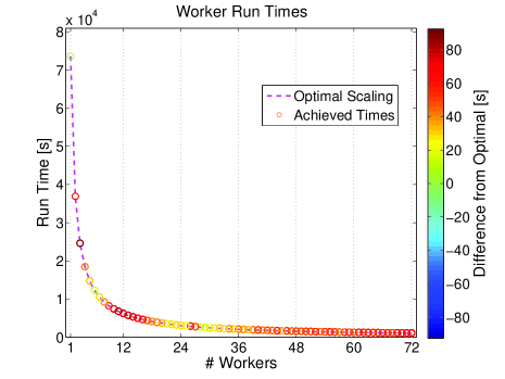
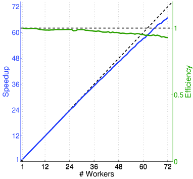
Scaling tests of Paramotopy were performed using the Monks equations, on a mesh of 48 points in each of three parameters, for a total of 110592 parameter points. Using the timing results from one worker as a base for calculation, we ran the same parameter sampling using identical , with up to 72 workers. Figure 4 shows the results. We saw great linear scaling throughout the tested range, with speedup and efficiency dropping off slightly as the number of workers approached 72. The trajectory of the two curves indicates that Paramotopy would have scaled to well over 72 processors.
We note here that scaling results depend on the problem size. In general, the larger the parameter sampling, the more processors one can be use. To be able to handle larger problems, Paramotopy has tunable settings for buffering memory in data collection, and parameter point distribution.
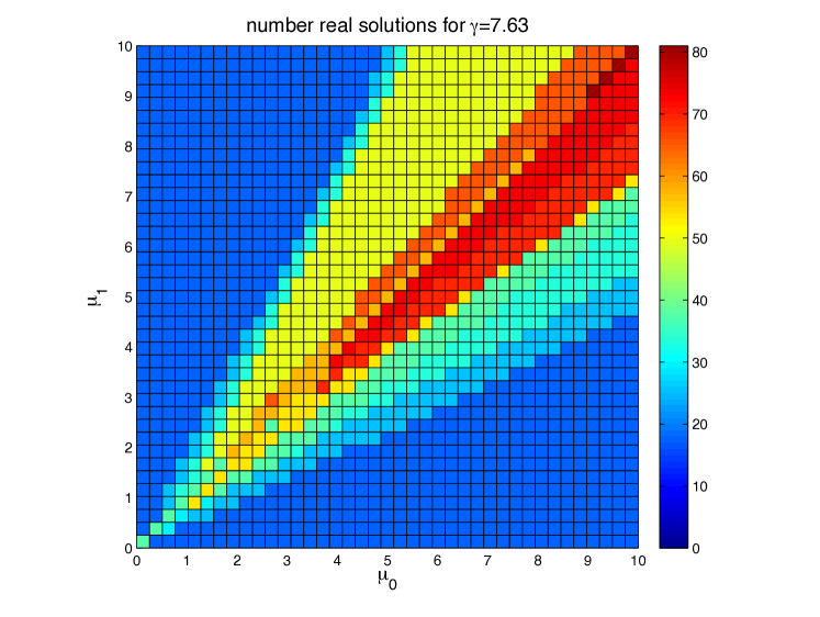
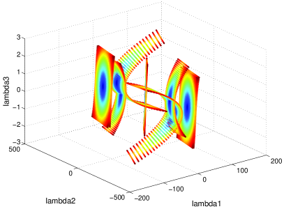
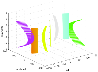
Aside from timing results, Paramotopy is useful in describing the dependence on the number of real equilibria in the system in relation to the values of the parameters, as seen in Figure 5. For generic parameter values, the Monks Equations have 81 distinct isolated complex solutions, with no positive-dimensional components in the variety corresponding to equilibria solution, as verified using a positive dimensional run in Bertini. Rarely enough, the single variable group total degree start system constructed by Bertini happens to have 81 paths to track as well. In this figure, we see one slice along in the three dimensional parameter space, with .
4.3 Control
The following system is derived from a receding horizon optimization problem, concerned with driving a nonlinear Duffing oscillator to rest [13]. The problem depends on parameters, and can be formulated as a polynomial system, for which we desire the roots. Paramotopy was designed specifically to solve such a system at multiple parameter points of interest. We will use one particular version of the system, corresponding to looking two steps ahead. The system is given below in Input 3.
Timing runs using a mesh of points are demonstrated in Figure 6. Again, linear speedup was achieved with efficiency of nearly one throughout the range of processors. The head spends most of its time waiting for the workers to ask for more work, and the trends in the timing indicate that Paramotopy in this case would have scaled well beyond 72 workers.
4.4 Path failure
To demonstrate the capabilities of Paramotopy to deal with path failures, we present here the results of a run using the ‘cube’ system:
| (2) |
Treating , as parameters, and letting be the sole variable, we get a one-variable system. See Input 4.
Discretizing in a 200x200 grid, for a total of 40,000 points, and solving using the default Bertini configuration, exactly four parameter points result in path failures:
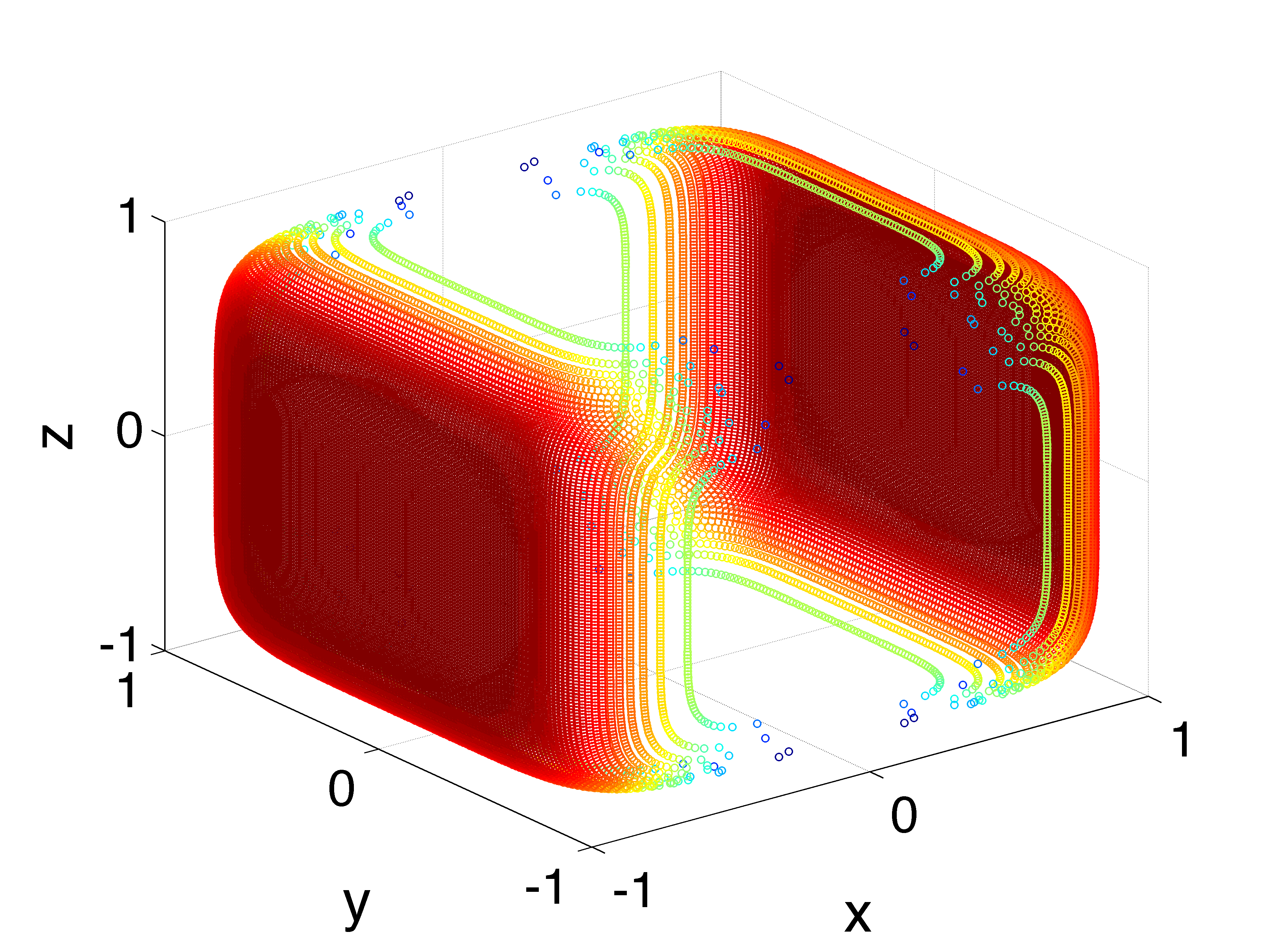
Paramotopy re-solved these points, by first moving the random complex start parameter values to another point , and then tracking to these four points, using a larger maxnorm (the maximum infinity-norm value of a solution at any point during Bertini solve), and securitylevel 1. Of course, whether to move to a new is determined by the user, as are the tolerance values and other Bertini settings. A plot of the solutions found, concatenated with the parameter values used to give a triple of coordinates, is presented in Figure 8.
One of the benefits of having automatic path failure detection and solution methods is speed. Solution of the system for all parameter values at the tighter tolerances would have taken much longer; it can be more time efficient to run at lower tolerances for a first pass, and re-solve with more secure settings only when and where needed.
5 Conclusions
In this article, we described the new open-source software package Paramotopy, which can be used to solve parameterized polynomial systems very efficiently for large numbers of parameter values. This extends the reach of numerical algebraic geometry in a new direction, particularly a direction that might be useful for mathematicians, scientists, and engineers who would like to rapidly test a hypothesis or would like to find regions of a parameter space over which the polynomial system has the same number of solutions. While Bertini and PHCpack have some parameter homotopy capabilities, Paramotopy has been optimized for the scenario of using many-processor computers to solve at many parameter values of interest.
Paramotopy is under ongoing development, and we expect several extensions in the coming months and years. For example, Bertini has been improved since the initial development of Paramotopy began in 2010. In particular, Bertini now has configuration settings to turn off parsing (Paramotopy currently uses a special version of Bertini built before this new configuration was added), and the parameter homotopy functionality of Bertini has now been expanded to include the use of projective space.
Also, we intend to expand Paramotopy to automatically search for and map out boundaries between cells of the parameter space within which the parameterized polynomial system has the same number of real solutions. More precisely, the discriminant locus of a parameterized polynomial system breaks the parameter space into cells. For all points within the same cell, the parameterized polynomial system has the same number of real solutions. By taking a grid within some region of the parameter space, successive refinements of this grid near parameter values for which solutions are ill-conditioned will help us to “zoom in” on portions of the discriminant locus. This “zooming in” procedure is currently under development and will provide a fast, numerical way of finding these boundaries. Currently, such boundaries can only be computed algebraically (this computation breaks down for systems of even moderate size) or through subdivision methods (which have difficulty in zooming in on positive-dimensional solution sets such as the discriminant locus).
In the numerical analysis of dynamical systems, significant research has been devoted to the computation of bifurcation points. MATCONT is a MATLAB package for the bifurcation analysis of ODEs [11]. Another software package for bifurcation analysis is DDE-BIFTOOL [12]. Both these packages are similar to some of the capabilities of Paramotopy but both packages are remarkably different from Paramotopy in scope and intended use. Both of these packages include continuation techniques over . Paramotopy is significantly different as it performs continuation methods over and works for general polynomial systems.
Acknowledgments
The authors would like to thank the useful comments from several anonymous referees and Andrew Sommese, which have greatly contributed to a better paper. The first author would also like to recognize the hospitality of Institut Mittag-Leffler and the Mathematical Biosciences Institute.
Appendix A Example input files
This appendix contains the input files for the four examples contained above in Section 4.
References
- [1] D. J. Bates, J. D. Hauenstein, and A. J. Sommese. Efficient path tracking methods. Numer. Algorithms, 58(4):451–459, 2011.
- [2] D. J. Bates, J. D. Hauenstein, and A. J. Sommese. A parallel endgame. Contemp. Math., 556:25–35, 2011.
- [3] D. J. Bates, J. D. Hauenstein, A. J. Sommese, and C. W. Wampler. Stepsize control for path tracking. Contemp. Math., 496:21–31, 2009.
- [4] D. J. Bates, J. D. Hauenstein, A. J. Sommese, and C. W. Wampler. Numerical solution of polynomial systems using the software package Bertini. SIAM, Philadelphia, PA, 2013.
- [5] D. J. Bates, J. D. Hauenstein, A. J. Sommese, and C.W. Wampler. Bertini: Software for numerical algebraic geometry, 2006.
- [6] D.J. Bates, J.D. Hauenstein, C. Peterson, and A.J. Sommese. A numerical local dimension test for points on the solution set of a system of polynomial equations. SIAM J. Numer. Anal., 47(5):3608–3623, 2009.
- [7] D.J. Bates, J.D. Hauenstein, A.J. Sommese, and C.W. Wampler. Adaptive multiprecision path tracking. SIAM J. Numer. Anal., 46(2):722–746, 2008.
- [8] D. A. Brake, D. J. Bates, V. Putkaradze, and A. A. Maciejewski. Illustration of numerical algebraic methods for workspace estimation of cooperating robots after joint failure. In 15th IASTED Int. Conf. on Rob. and Appl., pages 461–468, 2010.
- [9] D. A. Brake, D. J. D. J. Bates, W. Hao, J. D. Hauenstein, A. J Sommese, and C. W. Wampler. Algorithm 976: Bertini_real: Numerical decomposition of real algebraic curves and surfaces. ACM Transactions on Mathematical Software (TOMS), 44(1):10:1–10:30, July 2017.
- [10] J. Denavit and R.S. Hartenberg. A kinematic notation for lower-pair mechanisms based on matrices. Trans. ASME J. Appl. Mech., 23:215–221, 1955.
- [11] A. Dhooge, W. Govaerts, and Y.A. Kuznetsov. Matcont: a matlab package for numerical bifurcation analysis of odes. ACM Transactions on Mathematical Software (TOMS), 29(2):141–164, 2003.
- [12] K. Engelborghs, T. Luzyanina, and D. Roose. Numerical bifurcation analysis of delay differential equations using dde-biftool. ACM Transactions on Mathematical Software (TOMS), 28(1):1–21, 2002.
- [13] I. A. Fotiou, P. Rostalski, B. Sturmfels, and M. Morari. An algebraic geometry approach to nonlinear parametric optimization in control. In American Control Conference, 2006, pages 3618–3623, june 2006.
- [14] G.-M. Greuel, C. Stussak, M. Urbannek, A. Matt, A. Hartkopf, C. Knoth, H. Hauser, M. Alberich, J. Buend a, C. Corrales, L. May, A. Sabater, E. Sànchez, and O. Labs. Surfer. Technical report, 2011. http://imaginary.org/program/surfer.
- [15] J.D. Hauenstein, A.J. Sommese, and C.W. Wampler. Regeneration homotopies for solving systems of polynomials. Math. Comput., 80(273):345–377, 2010.
- [16] J.D. Hauenstein and C.W. Wampler. Isosingular sets and deflation. Foundations of Computational Mathematics, 13:371–403, 2013.
- [17] Yang-Hui He, Dhagash Mehta, Matthew Niemerg, Markus Rummel, and Alexandru Valeanu. Exploring the potential energy landscape over a large parameter-space. Journal of High Energy Physics, 2013(7):1–29, 2013.
- [18] S. Holzer and OliverLabs. surfex 0.90. Technical report, University of Mainz, University of Saarbrücken, 2008. www.surfex.AlgebraicSurface.net.
- [19] E. Lee and C. Mavroidis. Solving the geometric design problem of spatial 3R robot manipulators using polynomial homotopy continuation. J. Mech. Des., 124:653–661, December 2002.
- [20] A. Leykin, J. Verschelde, and A. Zhao. Newton’s method with deflation for isolated singularities of polynomial systems. Theoretical Computer Science, 359:111–122, 2006.
- [21] T. Y. Li. Numerical solution of polynomial systems by homotopy continuation methods. Handb. Numer. Anal., 11:209–304, 2003.
- [22] T. Y. Li, T. Sauer, and J. A. Yorke. The cheater’s homotopy: An efficient procedure for solving systems of polynomial equations. SIAM J. Numer. Anal., 26(5):1241–1251, 1989.
- [23] A. P. Morgan, A. J. Sommese, and C. W. Wampler. Computing singular solutions to polynomial systems. Adv. Appl. Math., 13(3):305–327, 1992.
- [24] A. P. Morgan, A. J. Sommese, and C. W. Wampler. A power series method for computing singular solutions to nonlinear analytic systems. Numer. Math., 63(1):391–409, 1992.
- [25] A. J. Newell. Transition to superparamagnetism in chains of magnetosome crystals. Geochem. Geophys. Geosy., 10(11):Q11Z08, 2009.
- [26] P. Rostalski, I. A. Fotiou, D. J. Bates, A. G. Beccuti, and M. Morari. Numerical algebraic geometry for optimal control applications. SIAM J Optimiz., 21(2):417–437, 2011.
- [27] A. J. Sommese and C. W. Wampler. The Numerical solution of systems of polynomials arising in engineering and science. World Scientific Publishing, 2005.
- [28] A.J. Sommese and A.P. Morgan. Coefficient-parameter polynomial continuation. Appl. Math and Comp., 29:123–160, 1989.
- [29] J. Verschelde. Algorithm 795: Phcpack: A general-purpose solver for polynomial systems by homotopy continuation. ACM Transactions on Mathematical Software (TOMS), 25(2):251–276, 1999.
- [30] C. W. Wampler. Bezout number calculations for multi-homogeneous polynomial systems. Appl. math. and comput., 51(2):143–157, 1992.