Interdependent Gibbs Samplers

Abstract

Gibbs sampling, as a model learning method, is known to produce the most accurate results available in a variety of domains, and is a de facto standard in these domains. Yet, it is also well known that Gibbs random walks usually have bottlenecks, sometimes termed “local maxima”, and thus samplers often return suboptimal solutions. In this paper we introduce a variation of the Gibbs sampler which yields high likelihood solutions significantly more often than the regular Gibbs sampler. Specifically, we show that combining multiple samplers, with certain dependence (coupling) between them, results in higher likelihood solutions. This side-steps the well known issue of identifiability, which has been the obstacle to combining samplers in previous work. We evaluate the approach on a Latent Dirichlet Allocation model, and also on HMM’s, where precise computation of likelihoods and comparisons to the standard EM algorithm are possible.

1 Introduction

Gibbs sampling is a standard model learning method in Bayesian Statistics, and in particular in the field of Graphical Models, [Gelman et al., 2014]. In the Machine Learning community, it is commonly applied in situations where non sample based algorithms, such as gradient descent and EM are not feasible. Perhaps the most prominent application example is the Latent Dirichlet Allocation (LDA) topic model [Blei et al., 2002], a model that is routinely used in text analysis, recommender systems, and a variety of other domains. For LDA, Gibbs sampling is considered to be the standard and the most accurate approach (see, for instance, [Smola and Narayanamurthy, 2010], [Papanikolaou et al., 2017]).

1.1 Local Maxima

The standard asymptotic theory of random walks guarantees that Gibbs, and more generally, MCMC samplers, eventually produce a sample from the target distribution (see [Gelman et al., 2014]). The number of steps of the sampler that is required to approximate well a sample from the target distribution is known as the mixing time of the sampler. However, it is well known to practitioners that the true mixing times of Gibbs samplers in realistic situations are unpractically high. The typical observed behavior of the random walk is not that one obtains a fresh sample from the target distribution every given number of steps, but rather that the walk converges to a certain configuration of the parameters, and stays in the vicinity of these parameters for extremely long times, which would not have had happened if mixing times where short. This is illustrated in Figure 1, and a related discussion is given in Section 4.1.

In view of this behavior, it is natural to ask how one can improve the quality of the solutions obtained as the local maxima. The simplest classical receipt is to run the sampler multiple times independently, and to choose the best solution. Note that it is usually not clear that running a sampler a few or even a few hundred times will significantly improve the quality of a solution. Moreover, in some situations, such as LDA, even the task of computing the quality of the solution (the loglikelihood in this case) is hard and can not be performed reliably.

Another approach would be to attempt to combine multiple solutions, to produce a single improved solution. However, while this general idea was discussed already in [Griffiths and Steyvers, 2004], at present there is no known way to carry this out, due to an issue known as the identifiability problem. In the next section we introduce the approach taken in this paper, and its relation to identifiability.

1.2 Mulitpaths and Identifiability

The approach of this paper, which we call the multipath sampler, is to use multiple, interdependent Gibbs samplers.

Consider a Bayesian setting where we a have generative model for the observed data $w=(w_{1},\ldots,w_{N})$ and a set of latent variables $p=(p_{1},\ldots,p_{N})$. The model depends on a set of parameters $\phi$, and this set is endowed with a prior, $\mathbb{P}\left(\phi\right)$. We call the set of latent variables a path. For LDA, $\phi$ corresponds to topics, with a Dirichlet prior, and for every token $w_{i}$, $i\leq N$, $p_{i}$ is the topic assigned to that token. In a standard (partially collapsed) Gibbs sampler one first samples the parameters from $\mathbb{P}\left(\phi|p,w\right)$, and then samples topic assignments $p_{i}$, from $\mathbb{P}\left(p_{i}|p_{-i},w,\phi\right)$, for each $i\leq N$. Here $p_{-i}$ are the values of all the assignments in the path except $p_{i}$.

In the multipath sampler, instead of a single set of latent variables $p$ we maintain $m$ sets, $p^{1},\ldots,p^{m}$. We define an appropriate joint distribution on them as described in Section 3. Under this joint distribution, the marginal distribution $p^{j}$ for each $j\leq m$ given the data $w$, coincides with the distribution of latent variables $p$ in the regular Gibbs sampler.

Next, to sample the latent variables $p^{j}$, we first sample $\mathbb{P}\left(\phi|p^{1},\ldots,p^{m},w\right)$, and then use the usual Gibbs sampler independently for each $p^{j}$, given $\phi$. The dependence between the paths $p^{j}$ is expressed in sampling from $\mathbb{P}\left(\phi|p^{1},\ldots,p^{m},w\right)$, where $\phi$ depends on all the $p^{j}$ together. This step can be viewed as model averaging. The details are given in Section 3. In particular, we will show that the target distribution of the multipath sampler emphasizes the solutions that have high likelihood for the regular sampler.

As noted earlier, the idea of model averaging in the context Gibbs sampling has been discussed in the literature at least since the paper [Griffiths and Steyvers, 2004]. In particular, it is well known that it is generally impossible to average the results of independent samplers, due to the problem of identifiability (see, for instance, [Griffiths and Steyvers, 2004], [Steyvers and Griffiths, 2007], [Gelman et al., 2014]), which refers to the issue that the model parameters are only defined by the model up to a permutation. For instance, in the case of LDA, suppose $\phi=(\phi_{1},\ldots,\phi_{T})$ and $\phi^{\prime}=(\phi^{\prime}_{1},\ldots,\phi^{\prime}_{T})$ are two sets of topics estimated by two independent Gibbs samplers. One then might attempt to combine $\phi_{1}$ and $\phi^{\prime}_{1}$, for instance by defining $\phi^{\prime\prime}_{1}=\frac{\phi_{1}+\phi^{\prime}_{1}}{2}$, to obtain a better estimate of the topic. However, even if $\phi$ and $\phi^{\prime}$ represent nearly the same set of topics, $\phi_{1}$ in $\phi$ does not necessarily correspond to $\phi^{\prime}_{1}$, but may rather correspond to some other $\phi^{\prime}_{j}$ for some $j\neq 1$. Thus, to perform direct averaging, one would have to find a proper permutation expressing the correspondence, before averaging. Moreover, the situation is further complicated by the fact that $\phi$ and $\phi^{\prime}$ do not necessarily represent similar sets of topics, and thus for many topics in $\phi$, there simply will be no “similar” topic in $\phi^{\prime}$ to average with.

With the multipath approach, we show for the first time how the identifiability problem can be avoided. Indeed, instead of running the samplers completely independently and attempting to only combine the final results, we allow the samplers to share the parameters during the optimization. This forces the samplers to find a common version of each topic, while still maintaining different and somewhat independent empirical estimates of it.

1.3 Experiments

We demonstrate the methods introduced in this paper on HMM and LDA Gibbs samplers, and in both cases the multipath sampler improves on the results of a regular sampler. We now motivate and briefly describe the experiments.

As mentioned earlier, in a typical problem where a Gibbs sampler is used, given the model parameters $\phi$ found by a sampler, there is no precise way to evaluate the likelihood of the data $w$ with respect to $\phi$. See [Wallach et al., 2009], where an equivalent notion of perplexity is discussed. As a result, it is not usually easy to compare two different solutions, $\phi$ and $\phi^{\prime}$, possibly found by two different methods, and perplexity, if used at all, is never used as a sole method of evaluation.

Therefore, to evaluate the performance of the multipath sampler we first compare it to the regular Gibbs sampler on a model where explicit computation of data likelihoods is possible. Specifically, we use Hidden Markov Models (HMMs), with synthetic data, where the parameters $\phi$ to be estimated are the emission and transition probabilities. We compare the solutions form the Gibbs samplers to those found by the EM-type Baum-Welch algorithm, and to the ground truth.

Next, we compare the Gibbs and the multipath Gibbs sampler LDA model on synthetic data and measure the closeness of the recovered topics to the ground truth.

In addition, on the well known State of The Union corpus, [Wang and McCallum, 2006], we compare the time concentration of the topics as an additional quality indicator. Specifically, this dataset consists of speeches given between the years 1790 to 2013, and each speech is further divided into multiple documents. When such time information is available, it is natural to ask whether certain topics appear in a specific time period, or their occurrence is spread relatively uniformly over time. We call a topic time-concentrated if most of its occurrences are contained in a short time period. Consider Figure 5 for an example of a relatively well time-concentrated topic.

Next, note that the LDA model itself has no access to timestamps, and that if token assignments were given at random, then the topics would be approximately uniformly spread over time. Therefore, time concentration of the topics may be observed only if the model fits the data well, and better time concentration implies a better fit to the data. In Section 4.2 we show that topics and topic assignments found by the multipath sampler have significantly better time-concentration properties compared to topics from the regular sampler.

We note that time concentration for topics is a well studied subject. For instance, the well known Topics over Time (ToT) model, [Wang and McCallum, 2006], and its numerous extensions, incorporate the timestamp data into the model via appropriate probabilistic constraints. These additional constraints may be viewed as an expression of a prior belief about the data, in particular that a topic’s usage pattern has certain temporal properties. Using such models, one indeed obtains topics that are better concentrated in time compared to standard LDA. However, note that by extending the model, one effectively forces a bias towards learning concentrated topics. In contrast, here we show that one can obtain improved concentration by an improved learning algorithm of LDA itself, without additional assumptions. This demonstrates that time-concentration of the topics is a signal contained in the data, rather than an artifact of the extended model.

The rest of the paper is organized as follows: In Section 2 we review the literature. In Section 3 we formally define the mulipath sampler and study its relation to the regular sampler. Section 4 contains the experiments, and concluding remarks and future work are discussed in Section 5.

2 Literature

A few days after the first posting of this paper, we have been informed that a similar approach has already been considered previously. While the experiments and the point of view taken in the discussion in this paper are different, the core idea, Algorithm 1, is identical to the algorithm introduced in [Doucet et al., 2002].

As detailed below, there is a large body of work on performance improvements for Gibbs samplers, and in particular for the Gibbs samplers of the LDA model.

The uncollapsed Gibbs sampler for LDA was introduced in [Pritchard et al., 2000] where it was applied to genetic data. The collapsed Gibbs sampler was introduced in [Griffiths and Steyvers, 2004].

Parallelization was studied, for instance, in [Newman et al., 2007], [Smola and Narayanamurthy, 2010]. In [Neiswanger et al., 2014] parallelization methods with asymptotical exactness guarantees were given. Note that while parallelizing the fully collapsed Gibbs sampler presents several significant issues which are addressed in the above work, for LDA there is a partially collapsed sampler, studied in [Asuncion, 2011], which is straightforward to parallelize. As observed in [Magnusson et al., 2017], the partially collapsed samplers may have a performance, in terms of quality of solutions, comparable to the performance of the fully collapsed sampler.

Methods that exploit sparseness of distributions to speed up the iteration of the sampler were studied, among other work, in [Yao et al., 2009], [Li et al., 2014], and further optimized in [Chen et al., 2016]. These methods perform the same random walk as the collapsed sampler, but the sampling step itself is implemented more efficiently.

In a recent work [Papanikolaou et al., 2017], parameter inference by averaging several solutions was discussed for the case of LDA. It is important to note here that this refers to a very restricted form of averaging. Indeed, in that work, one first obtains a solution from a collapsed Gibbs sampler, and a postprocessing step considers perturbations in this solution at a single coordinate, to obtain some variability in the assignment. Thus all the perturbed solutions differ from the original solution at a single coordinate at most. It is then argued that such perturbations can be averaged, since changing only one assignment coordinate in a large corpus is unlikely to cause the identifiability issues associated with averaging. Clearly, however, due to the same reasons, such perturbations can not change the particular local maxima of the original solution and can only provide small variations around it. Thus, while this approach is useful as a local denoising method, especially in computing topic assignment distributions (rather than topic themselves), and is suggested as such in [Papanikolaou et al., 2017], the overall quality of the solution is the same as the one returned by the original sampler. As discussed in the Introduction, our approach completely avoids the identifiability issues, and allows to combine information from significantly differing topic assignments.

Finally, we note that all of the above mentioned methods can be combined with the methods introduced in this paper. In particular both multipath samplers may be parallelized and may incorporate sparsity in exactly the same way this is done for the regular sampler.

3 Multiple Paths

We will assume that the data is generated in a standard Bayesian setting: A set of model parameters is denoted by $\Phi$, endowed with a prior distribution $\mathbb{P}\left(\phi\right)$. Given $\phi$, the model specifies a distribution of latent variables $p=\left(p_{i}\right)_{i=1}^{N}$, $\mathbb{P}\left(p|\phi\right)$. Each $p_{i}$ takes values in the set $\left\{1,\ldots,S\right\}$. By analogy to HMMs, we refer to the latent variables $p$ as a path, and denote the set of all possible values of a path sequence by $\mathcal{P}=\mathcal{P}_{N}=\left\{1,\ldots,S\right\}^{N}$.

Finally, given the parameters and the path, the model specifies the distribution of the observed variables $\mathbb{P}\left(w|p,\phi\right)$, where $w=\left(w_{i}\right)_{i=1}^{N}$. We also refer to $w$ as the data variables. Each $w_{i}$ takes values in the alphabet $\left\{1,\ldots,W\right\}$.

In the case of HMMs, the parameters $\phi$ are be the transition and emission distributions. Specifically, we consider HMMs with $S$ states, and with emissions given by discrete distributions on the alphabet $\left\{1,\ldots,W\right\}$. Then $\phi=(\beta^{\prime},\beta_{1},\ldots,\beta_{S},e_{1},\ldots,e_{S})$, where $\beta^{\prime}$ is the initial distribution on the Markov chain, for each $j\leq S$, $\beta_{j}$ is the transition distribution given the chain is at state $j$, and $e_{j}$ are emission distributions for state $j$. The prior is given by $\beta^{\prime}\sim Dir_{S}(1)$, $\beta_{j}\sim Dir_{S}(1)$, and $e_{j}\sim Dir_{W}(1)$. The path $p$ is a state sequence sampled from the Markov chain, and $w$ are the emissions given the state sequence, so that the distribution of given $p_{i}=j$ is $w_{i}\sim e_{j}$.

For LDA, the parameters are the topics, $\phi=(\phi_{1},\ldots,\phi_{S})$, with a prior $\phi_{j}\sim Dir_{W}(\eta)$, for some fixed $\eta>0$. The path is the set of topic assignments for each token in the corpus, and $w$ are the tokens, where $w_{i}$ is sampled from the topic $p_{i}$.

Next, the following definitions will be useful. We refer to the quantity

$$\mathbb{P}\left(w,p|\phi\right)$$ (1)

as the path likelihood, and to

$$\mathbb{P}\left(w|\phi\right)=\sum_{p\in\mathcal{P}}\mathbb{P}\left(w,p|\phi\right)$$ (2)

the data likelihood.

Given the data $w$, we interested in the maximum likelihood parameter values, $\phi_{max}$,

$$\phi_{max}=\operatornamewithlimits{argmax}_{\phi}\mathbb{P}\left(w|\phi\right),$$ (3)

and in a sample of $p$ given $w$ and $\phi_{\max}$. A standard approach to obtaining an approximation of $\phi_{max}$ is to use a Gibbs sampler to sample from $\mathbb{P}\left(\phi,p|w\right)$.

Now, on the set of parameters and paths, $\Phi\times\mathcal{P}$, define the function

$$f(\phi,p)=\mathbb{P}\left(w,p,\phi\right)=\mathbb{P}\left(w,p|\phi\right)\cdot\mathbb{P}\left(\phi\right).$$

Denote by

$$C_{f}=\sum_{p}\int_{\Phi}f(\phi,p)d\phi=\mathbb{P}\left(w\right),$$

where $d\phi$ is the Lebesgue measure on $\Phi$ (that is, $\mathbb{P}\left(\phi\right)$ is a density with respect to $d\phi$ ).

Then the probability density $\hat{f}(\phi,p)=\frac{1}{C_{f}}f(\phi,p)$ is, by definition, the density of the posterior distribution $\mathbb{P}\left(\phi,p|w\right)$.

Observe that the posterior density of $\phi$ is proportional to the data likelihood of $\phi$:

$$\hat{f}(\phi)=\sum_{p}\hat{f}(\phi,p)=\frac{1}{C_{f}}\sum_{p}\mathbb{P}\left(\phi,p,\mathcal{D}\right)=$$ (4)

$$=\frac{1}{C_{f}}\cdot\mathbb{P}\left(\phi\right)\cdot\mathbb{P}\left(w|\phi\right).$$

We are now ready to introduce the multiple paths model. The generative model consist of simply sampling the parameters $\phi$ from $\mathbb{P}\left(\phi\right)$, and then sampling $m$ independent copies of the paths, $p^{j}$, and the data, $w^{j}$. Here the data sequence $\left\{w_{i}^{j}\right\}_{i\leq N}$ is sampled from the original generative model given $\phi$ and $p^{j}$. Therefore, the model generates $m$ paths, and $m$ versions of the data. In what follows we will condition this model on the event that all the versions of the data coincide and are equal to a given data sequence $w$.

Specifically, given a data sequence $w$, we seek the posterior distribution of $\phi$ in the $m$ path model, given the data $w^{j}$, such that $w^{j}=w$ for all paths $j\leq m$.

For $m\geq 1$, define on $\Phi\times\mathcal{P}^{m}$ the function

$$f_{m}(\phi,p^{1},\ldots,p^{m})=\mathbb{P}\left(\phi\right)\cdot\prod_{j\leq m}\mathbb{P}\left(p^{j},w|\phi\right).$$ (5)

Denote by $C_{f_{m}}$ the corresponding normalization constant,

$$C_{f_{m}}=\int_{\Phi}\sum_{p^{1},\ldots,p^{m}}f_{m}(\phi,p^{1},\ldots,p^{m})d\phi.$$

Then $\hat{f}_{m}=\frac{1}{C_{f_{m}}}f_{m}$ gives the distribution of $(\phi,p^{1},\ldots,p^{m})$ with respect to the multipath generative model, conditioned on the event $w^{j}=w$ for all $j\leq m$.

The following observation is the key fact of this section, and we record it as a lemma.

Lemma 3.1.

Let $(\phi,p^{1},\ldots,p^{m})$ be a sample from $\hat{f}_{m}$. Then the marginal density of $\phi$ is

$$\mathbb{P}_{m}\left(\phi|w\right)=\frac{1}{C_{f_{m}}}\mathbb{P}\left(\phi\right)\mathbb{P}\left(w|\phi\right)^{m}.$$ (6)

Proof.

Indeed,

$$C_{f_{m}}\cdot\mathbb{P}_{m}\left(\phi|w\right)=\sum_{p^{1},\ldots,p^{m}}f_{m}(\phi,p^{1},\ldots,p^{m})=$$

$$\mathbb{P}\left(\phi\right)\sum_{p^{1},\ldots,p^{m}}\prod_{j\leq m}\mathbb{P}\left(p^{j},w|\phi\right)=$$

$$\mathbb{P}\left(\phi\right)\prod_{j\leq m}\sum_{p^{j}}\mathbb{P}\left(p^{j},w|\phi\right)=$$

$$\mathbb{P}\left(\phi\right)\mathbb{P}\left(w|\phi\right)^{m}.$$

∎

Note that this generalizes (4). The crucial detail about (6) is that it contains the $m$-th power of the data likelihood. Let $\phi_{max}$, defined in (3), be a maximum likelihood solution given the data, and let $\phi$ be any other parameter. Then,

$$\mathbb{P}_{m}\left(\phi_{max}|w\right)\big{/}\mathbb{P}_{m}\left(\phi|w\right)=$$

$$\left(\mathbb{P}\left(w|\phi_{max}\right)\big{/}\mathbb{P}\left(w|\phi\right)\right)^{m}=$$

$$\left(\mathbb{P}\left(\phi_{max}|w\right)\big{/}\mathbb{P}\left(\phi|w\right)\right)^{m}.$$

In words, we are exponentially more likely to obtain $\phi_{max}$ as a sample form $\hat{f}_{m}$ than from $\hat{f}$ (compared to any other $\phi$). Thus, as $m$ grows, any sample form $\hat{f}_{m}$ should yield $\phi$ with data likelihood close to that of $\phi_{max}$.

The discussion above shows why sampling from $\hat{f}_{m}$ yields better solutions than sampling from $\hat{f}$. We now discuss the Gibbs sampler for $\hat{f}_{m}$, which is a straightforward extension of the sampler for $\hat{f}$. The sampler is given schematically in Algorithm 1. For $m=1$, this is the standard Gibbs sampler.

The notation $p_{-i}$ has the standard meaning of $p$ without the $i$-th component $p_{i}$. For the $m$-path model, our path is the collection of all paths $p^{1},\dots,p^{m}$. However, when sampling and individual component $p_{i}^{j}$ from $p^{j}$, since the density (5) factorizes over $j$, we obtain:

$$\mathbb{P}\left(p_{i}^{j}=s|p_{-i}^{j},p^{1},\ldots,p^{j-1},p^{j+1},\ldots,p^{m},w,\phi\right)=$$

$$\mathbb{P}\left(p_{i}^{j}=s|p_{-i}^{j},w,\phi\right)$$

for every $s\in S$. Thus, given the parameters $\phi$, one samples each path $p^{j}$ independently from the others.

Algorithm 1 Multi path Gibbs Sampler

1:  Input: Data $w$ of length $N$, number of paths $m$.

2:  Initialize paths $p^{1},\dots,p^{m}$ at random.

3:  repeat

4:     Sample $\phi$ from $\mathbb{P}\left(\phi|p^{1},\ldots,p^{m},w\right)$.

5:     for all  $i\leq N$ do

6:        for all  $j\leq m$ do

7:           Sample $p_{i}^{j}$ from $\mathbb{P}\left(p_{i}^{j}|p_{-i}^{j},w,\phi\right)$.

8:        end for

9:     end for

10:  until  iteration count threshold is reached.

For the special cases of HMM and LDA, we write out Algorithm 1 in full detail in Supplementary Material Section B. In particular, we detail the equations which describe how steps 4 and 7 of Algorithm 1 are performed for these models. As mentioned earlier, these equations are straightforward modifications of the corresponding equations for the standard sampler. Also, note that for LDA, Algorithm 1 corresponds to the so called partially collapsed Gibbs sampler, rather than to the more common fully collapsed version. However, a fully collapsed version of a sampler from $\hat{f_{m}}$ is equally easy to derive, and is also presented in Supplementary Material Section B.

As discussed above, the advantage of the multipath sampling comes from the fact that it implicitly samples $\phi$ from a distribution proportional to $\mathbb{P}\left(\phi|w\right)^{m}$. Note that while $\mathbb{P}\left(\phi|w\right)$ is not typically computable, the path likelihood $\mathbb{P}\left(\phi,p|w\right)$ is computable. It is then natural to ask what will happen if the Gibbs sampler is modified to sample the pair $(\phi,p)$ from a distribution proportional to $\mathbb{P}\left(\phi,p|w\right)^{m}$. This can easily be accomplished, using a single path. Such a sampler will spend much more time around the pairs $(\phi,p)$ for which $\mathbb{P}\left(\phi,p|w\right)$ is high, compared to the regular Gibbs sampler. However, even if we were given a pair $(\phi^{\prime},p^{\prime})$ that maximizes $\mathbb{P}\left(\phi,p|w\right)$ globally over all $\phi,p$, it is straightforward to verify that $\phi^{\prime}$ would not usually correspond to useful parameters. On the other hand, if the data is generated by a model with parameters $\psi$, then consistency results (such as, for instance, [Baum and Petrie, 1966] for the case of HMMs) ensure that maximum data likelihood solutions, as in (3), reconstruct $\psi$. The important feature of multipath sampler is therefore that it samples from $\mathbb{P}\left(\phi|w\right)^{m}$, even though $\mathbb{P}\left(\phi|w\right)$ is not computable.

Finally, it is worthwhile to remark that the multipath approach bears some resemblance to the EM algorithm. Indeed, in EM algorithm, for each $i\leq N$, one computes the distribution of $p_{i}$ given all the data $w$ and parameters $\phi$. Then, given these distributions, one recomputes the parameters. One can view the multipath scheme as an approximation of the $p_{i}$ distribution with $m$ samples, instead of a computation of it in a closed form as in EM, or an approximation with one sample, as in regular Gibbs. A substantial difference between EM and the sampler is that our samples of $p_{i}$ are conditioned on the data and the rest of the assignments, $p_{-i}$, while in EM the distribution is conditioned only on the data. However, interestingly, note that if the assignments $p_{i}$ are independent given the parameters, as in the case of mixture models, than a multipath sampler directly approximates EM as $m$ grows.

4 Experiments

In this Section we describe the HMM and LDA experiments. In addition, in Section 4.1, after describing the HMM experiments we discuss Figure 1, referred to in Section 1, which demonstrates the local maxima behavior of the Gibbs sampler.

4.1 HMMs

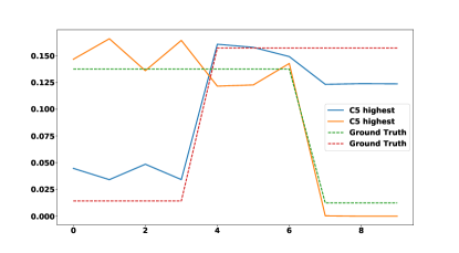
The HMM experiments use synthetic data. The data was generated by an HMM with two states, such that the transition probability between the states is $0.45$, and the emissions are distributions on $W=10$ symbols. The emissions are show in Figure 3 as the ground truth. All the experiments were conducted using the same fixed random sample of size $N=200000$ from this HMM.

These particular parameters were chosen in order to make the HMM hard to learn. Otherwise, all methods would succeed all the time, and would be difficult to compare. This corresponds to realistic situations where different emissions are hard to distinguish.

Note that while $N=200000$ may appear as a high number of samples, in this case, due to transitions probabilities which are close to $0.5$, this high number of samples is in fact necessary. As we discuss later, even with this number of samples, both the EM algorithm and some runs of the Gibbs sampler manage to slightly overfit the solution.

To put the HMM learning problem in the Bayesian setting, we endow the set of parameters with a prior where transition and emission distributions are sampled from a uniform Dirchlet, $Dir(1)$. In other words, transition distributions are sampled uniformly from a 3-simplex, and emission distributions from an 11-simplex. The data $w$ is the given emissions of the HMM, and the path $p$ corresponds to the latent sequence of the states of the HMM.

Figure 1 demonstrates the local maxima behavior. It shows the data log-likelihoods of a solution along a run of a collapsed Gibbs sampler, for 16 independent runs of a collapsed Gibbs sampler.

Each run had 200000 iterations, with data log-likelihoods computed every 100 iterations. As discussed in the Introduction, each run converges fairly quickly to an area of fixed likelihood, and stays there for extremely long time intervals.

Figure 1: Collapsed Gibbs HMM Data Likelihoods, illustrating the Local Maxima. Measurement is performed every 100 iterations. Total of 200000 iterations.

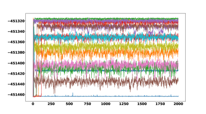
Figure 2 shows the data log-likelihoods of the parameters $\phi$ for multiple runs of different algorithms after 200000 iterations. Each algorithm was run independently 16 times (all on the same data), and the resulting data log-likelihoods are plotted in ascending order. The algorithms included are the Collapsed Gibbs sampler for 1 and five paths (C 1, 5) and a non-collapsed sampler (PC 1, 5).

For reference, the constant line (BW) corresponds to a solution found by the Baum-Welch algorithm, and Ground line corresponds to the data likelihood for the ground truth parameters. Note that the Ground line is slightly lower than the highest likelihood solutions, even with the relatively high number of samples $N=200000$.

Figure 2: Data likelihoods, all algorithms

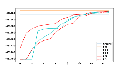
Clearly most of the algorithms improve on the base-line – the Collapsed Gibbs sampler C1. The the non- collapsed sampler, PC1, which is also a base-line, provides results similar to those of C1. The best results are obtained by C 5. The emissions found by C5 run with the highest data likelihood are shown in Figure 3. Note that the imperfect approximation of the emissions may be explained by a mild overfitting due to the barely sufficient amount of data.

Figure 3: Emissions of highest C5

4.2 LDA

In this Section we describe the LDA experiments.

4.2.1 Synthetic Data

The $T=10$ topics for the synthetic data are shown in Figure 4. They were constructed as follows: Choose 10 overlapping bands of equal length (except the boundary ones) on a dictionary of size $W=100$, centered at equally spaced intervals over $0,\ldots,99$. Each topic is a linear combination of a band, with weight $0.95$ and a uniform distribution on $W$, with weight $0.05$. Most of the points in the dictionary belong to two topics (if one disregards the uniform component present in all topics).

Figure 4: LDA Synthetic Topics

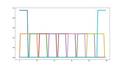
Each document is generated by sampling the topic distribution $\theta\sim Dir(\alpha)$, with $\alpha=1$, and sampling 10 tokens by sampling a topic from $\theta$, and a token from that topic.

We have generated a varying number of documents from this model, and have run the collapsed LDA Gibbs sampler with a varying number of paths. Given the topics $\beta_{1},\ldots,\beta_{10}$ found by the sampler, to compute a distance to ground truth,$disc$, for each ground truth topic $\beta^{g}_{i}$, we find a topic $\beta_{j}$ closest to $\beta^{g}_{i}$ in total variation distance, and take the mean of these distances:

$$disc=\frac{1}{10}\sum_{i}\min_{j}\left\|\beta^{g}_{i}-\beta_{j}\right\|_{1}$$

In addition, each $disc$ was averaged over 10 independent runs of the sampler (with same data and same number of paths). Samplers with different number of sources, but same number of documents, were run on the set of documents. All samplers were run for 10000 iterations, and in all cases already after 3000 the topics stabilized and practically did not change further. The results are shown in Table 1. Clearly, increasing the number of paths yields better reconstruction. Increasing the number of paths to more than 5 improved the performance further in some, but not all cases.

Table 1: Topic reconstruction results for synthetic LDA data, for varying number of paths and documents

$m$ (paths num.)	1500	3000	6000	9000
1	1.12	0.79	0.58	0.43
2	0.86	0.59	0.41	0.32
3	0.77	0.54	0.35	0.29
5	0.69	0.46	0.31	0.24

4.2.2 SOTU Dataset

Our State of the Union speeches corpus contains speeches from years 1790 to 2013. The preprocessing included stop words removal, stemming, removal of 40 most common words, and words that appeared only once in the corpus. Each speech was divided into paragraphs, and each paragraph was treated as a document. After the preprocessing, the corpus contains around 767000 tokens, in about 21000 documents. There are on average 50-80 documents corresponding to a single year. All the models were fit with $T=500$ topics and prior parameters $\eta=0.01$ and $\alpha=10/T=0.02$.

As discussed in Section 1.3, we compare the time- concentration properties of LDA models on the State of the Union corpus, found by the collapsed Gibbs sampler (referred to as LDA in what follows), and by multipath collapsed Gibbs sampler with $m=5$ paths (to which we refer as mpLDA). We quantify the time concentration of topics in two different ways, via the computation of yearly entropy, and via the notion of quantile buckets, as discussed below.

Given the topic assignments $p$ returned by the sampler, we compute several quantities as discussed below. For each document $d$, let $\theta_{d}$ be the topic distribution ( a probability distribution on the set $0,\ldots,T-1$) of the document, as computed by the sampler. Specifically, if $i_{1}^{d},\ldots,i_{k}^{d}$ are the indexes of the tokens in a document $d$, with $k=\left|d\right|$ the size of the document, then

$$\theta_{d}=\frac{1}{k}\sum_{l\leq k}\delta_{p_{i_{k}^{d}}}.$$

For the multipath sampler, we take the assignments from the first path $p^{1}$, for convenience. Typically, after convergence, for most tokens, all paths have an identical assignment for a given token.

Next, for each year, we compute the topic distribution: Let $\mathcal{Y}_{y}$ be the set of documents from year $y$. Then the topic distribution of the year $y$ is

$$\theta_{y}=\frac{1}{\left|\mathcal{Y}_{y}\right|}\sum_{d\in\mathcal{Y}_{y}}\theta_{d}.$$

We refer to $\theta_{y}(t)$ as the topic weight of topic $t$ for year $y$. The Figure 5 shows in blue the topic weights for all years of a particular topic $t$ in a model found by the collapsed Gibbs sampler. The 9 words with highest probabilities in this topic are indicated in the figure. In addition, we have found the topic $t^{\prime}$ in the model returned by the Mulipath Gibbs, and $t^{\prime\prime}$ for the aternating sampler which are closest to $t$ in total variation distance (as distributions over words). The topic weights of $t^{\prime}$ and $t^{\prime\prime}$ are shown in orange and green.

Figure 5: Topic Comparison LDA/mpLDA

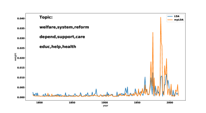
As Figure 5 shows, the orange curve has more weight on the years where both blue and orange curves have high values, and it has less weight in other areas. Note that the second statement here (less weight) does not follow from the first (more weight) – the weight of the topic over the years does not have to sum to 1 (the sum over all topics for a fixed year is 1). We conclude that the orange topic is more time concentrated than the blue. Similar conclusion also holds for the green topic.

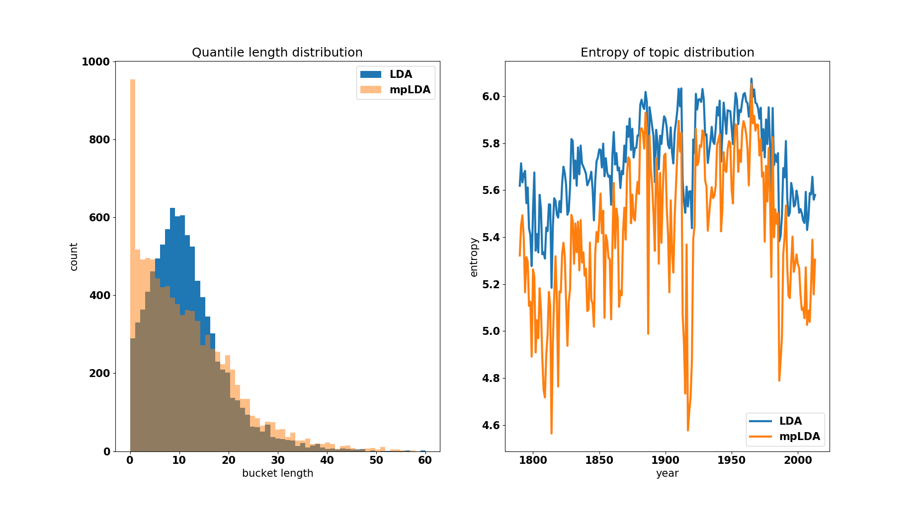
We now proceed to show that the situation depicted in Figure 5 for a fixed topic, is in fact typical for most topics, and overall the topics of mpLDA are better concentrated than those of LDA. First, consider the entropy of the topic distribution $\theta_{y}$ for every year, for all models, as shown in Figure 7 (right). The entropies of mpLDA are similar consistently lower than those of LDA for every year. This means that each year in the new models is composed of slightly fewer topics, with higher weights.

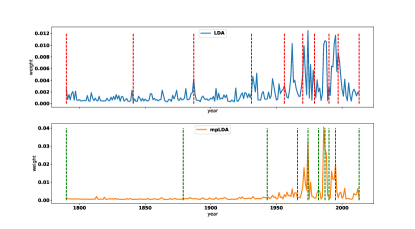
Second, given the topic weights for a fixed topic, we quantify its time concentration via the notion of quantile bucket length. A $\gamma$-quantile bucket of the weights is a time interval which contains a $\gamma$ proportion of the total weight of the topic. For instance, Figure 6 show $\gamma=0.1$ quantile buckets for topics from Figure 5. Shorter buckets mean that a fixed proportion of the weight is contained in a shorter time interval. Note that the short buckets of the orange curve in Figure 6 are shorter than than those of the blue curve.

Figure 6: $0.1$-quantile buckets

In Figure 7 (left), the distribution of the bucket lengths, with $\gamma=0.05$, for all the buckets from all the topics is shown, for all models. Since the sum of each 20 buckets contributed by a single topic is 224, the total number of years, the expectation of each histogram must be $11.2$. We observe that the blue histogram is centered around this value, indicating more or less uniform (over time) weight distributions for most of the topics of LDA. On the other hand, the orange histogram is clearly skewed to the left, which implies that there are more short intervals containing a fixed weight in mpLDA.

Some additional measurements related to this experiment may be found in Supplementary Material Section A.

Figure 7: Bucket Lengths and Yearly Entropies

5 Conclusion and Future Work

In this work we have introduced a modification of the Gibbs sampler, which combines samples from multiple sets of latent variables and yet avoids the identifiability problem. We have shown that asymptotically this sampler is exponentially more likely, compared to the regular Gibbs sampler, to return samples which have high data likelihood in the original generative model. We have also shown empirically that the quality of the solutions indeed improves, as the number of paths grows.

In addition, we found that time concentration properties of topic models may improve when using the multipath sampler, compared to regular Gibbs. This is one instance of a phenomenon where a better optimization of a model yields better insight into the data. However, full implications of this fact, in particular in the context of trend analysis, would require a more extensive investigation.

While we have tested our methods on the HMM and LDA models, our methods were formulated in a fairly generic latent variables settings, and could be extended even further. Thus, a natural direction for future work would be to understand the impact of the methods presented here on learning in other models, such as Markov Random Fields or extended HMMs with large state spaces, for which EM algorithms are not feasible.

Appendix A Additional Considerations Regarding Time Concentration

In Section 4.2.2 we have found that for topics and topic assignments from the multipath Gibbs sampler, the distribution of bucket lengths is more skewed to the left.

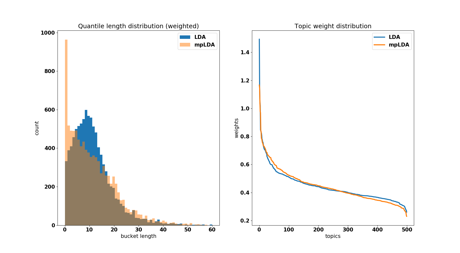
However, note that there might have existed degenerate topic assignments, which could have produced the concentration results of Figure 7. Indeed, consider an assignment where there is a single topic that is assigned to a major portion of every document, with the rest of the topics distributed in a concentrated way over the years. Such an assignment would lower the yearly entropy and produce a left skew in bucket lengths, but, arguably, should not be considered a better description of the data. To ensure that this is not the case, for each topic $t\leq T$, consider the total topic weight

$$w_{t}=\sum_{y}\theta_{y}(t).$$ (7)

In Figure 8, we show the sorted topic weights for both models (right) and the histogram of bucket lengths (left), where each bucket length is weighted proportionally to the topic weight $w_{t}$ of its topic (rather then by 1, as in computation for Figure 7). The topic weight distribution is practically the same for both models, and the lengths histograms also remain practically unchanged. This shows that the mpLDA genuinely redistributes the same topic weights in a more time concentrated fashion, rather than produces anomalous assignments.

Figure 8: Weighted Bucket Lengths, Topic Weights

Appendix B Explicit Implementations

In this Section we describe a fully detailed implementation of a multipath Gibbs sampler Algorithm 1 for LDA. As discussed in Section 3, in order to fully specify Algorithm 1 for a particular generative model, one has to implement the sampling in lines 4 and 7 of the Algorithm. Line 4 corresponds to line 6 in Algorithm 3, and line 7 to lines 12-19.

In addition, we describe the multipath analog of the collapsed Gibbs sampler. Schematically, the multipath collapsed Gibbs sampler is given in Algorithm 2, and Algorithm 4 is a full implementation.

The notation for the algorithms is summarized in Table 2, and is analogous to the one commonly used in the literature.

Note that for $m=1$ both Algorithm 3 and 4 coincide with their standard counterparts.

All computations in the derivation of the algorithms are standard Dirichlet conjugacy type computations. We omit the computations, since they are completely analogous to the computations for the derivation of the regular LDA Gibbs sampler. The algorithms for the HMM model are also derived using similar (slightly simpler) computations.

Please see the next page for the notation and the algorithms.

Algorithm 2 Multipath Collapsed Gibbs Sampler

1:  Input: Data $w$ of length $N$, number of paths $m$.

2:  Initialize paths $p^{1},\dots,p^{m}$ at random.

3:  repeat

4:     for all  $i\leq N$ do

5:        for all  $j\leq m$ do

6:           Sample $p_{i}^{j}$ from   $\mathbb{P}\left(p_{i}^{j}|p^{1},\ldots,p^{j}_{-i},\ldots,p^{m},w\right)$.

7:        end for

8:     end for

9:  until  iteration count threshold is reached.

Table 2: LDA Notation

Name	Description
Model Notation
$T$	Number of topics
$W$	Dictionary size
$m$	Number of paths in a multipath model
$\eta$	Hyperparameter for words in a topic
$\alpha$	Hyperparameter for topics in a document
$\beta_{i}$	Topics, $i\leq T$.
Corpus Notation
$N$	Total number of tokens in a corpus
$D$	Total number of documents in a corpus
$w_{i}$	The $i$-th token in a corpus. $i\leq N$ and $w_{i}\leq W\hskip 5.69054pt\forall i\leq N$
$\mathcal{D}_{i}$	The document of the $i$-th token in a corpus. $i\leq N$ and $\mathcal{D}_{i}\leq D\hskip 5.69054pt\forall i\leq N$
Sampler Notation
$p^{j}_{i}$	Topic assignment to the $i$-th word in a corpus. $i\leq N$,$j\leq m$ and $p^{j}_{i}\leq T\hskip 5.69054pt\forall i,j$
$\mathcal{C}^{TW}_{tw}$	Topic-word counter, $\mathcal{C}^{TW}_{tw}=\sum_{j\leq m}\left|\left\{i\leq N\hskip 5.69054pt|\hskip 5.69054ptw_{i}=w\wedge p^{j}_{i}=t\right\}\right|$
$\mathcal{C}^{T}_{t}$	Topic occurrence count, $\mathcal{C}^{T}_{t}=\sum_{w}\mathcal{C}^{TW}_{tw}$
$\mathcal{C}^{D}_{d}$	Document occurrence count (size of document $d$), $\mathcal{C}^{D}_{d}=\left|\left\{i\leq N\hskip 5.69054pt|\hskip 5.69054pt\mathcal{D}_{i}=d\right\}\right|$
$\mathcal{C}^{DT}_{jdt}$	Document-topic counter, $\mathcal{C}^{DT}_{jdt}=\left|\left\{i\leq N\hskip 5.69054pt|\hskip 5.69054pt\mathcal{D}_{i}=d\wedge p^{j}_{i}=t\right\}\right|$ with $j\leq m$

Algorithm 3 Multipath Partially Collapsed LDA Gibbs Sampler

1:  Input: Hyperparameters $\alpha,\eta$, data $\mathcal{W},\mathcal{D}$.

2:  Initialize $p^{j}_{i}$ to random integers in range $[1,T]$.

3:  Initialize $\mathcal{C}^{TW},\mathcal{C}^{DT},\mathcal{C}^{T}$ from $p$.

4:  repeat

5:     for all  $t\leq T$ do

6:        Sample $\beta_{t}\leftarrow Dir(\eta+\mathcal{C}^{TW}_{t,0},\ldots,\eta+\mathcal{C}^{TW}_{t,W-1})$

7:     end for

8:     for all  $j\leq m$ do

9:        for all  $i\leq N$ do

10:           $w\leftarrow w_{i}$, $d\leftarrow\mathcal{D}_{i}$.

11:           $z\leftarrow p^{j}_{i}$.

12:           $\mathcal{C}^{TW}_{zw}\leftarrow\mathcal{C}^{TW}_{zw}-1$,  $\mathcal{C}^{DT}_{jdz}\leftarrow\mathcal{C}^{DT}_{jdz}-1$,   $\mathcal{C}^{T}_{z}\leftarrow\mathcal{C}^{T}_{z}-1$.

13:           for all  $t\leq T$ do

14:              $r_{t}\leftarrow\beta_{t}(w)\cdot\left(\mathcal{C}^{DT}_{jdt}+\alpha\right)$.

15:           end for

16:           $r\leftarrow\sum_{t\leq T}r_{t}$.

17:           Sample $z^{\prime}\leftarrow multinomial\left(\frac{r_{1}}{r},\ldots,\frac{r_{T}}{r}\right)$.

18:           $p^{j}_{i}\leftarrow z^{\prime}$.

19:           $\mathcal{C}^{TW}_{z^{\prime}w}\leftarrow\mathcal{C}^{TW}_{z^{\prime}w}+1$,  $\mathcal{C}^{DT}_{jdz^{\prime}}\leftarrow\mathcal{C}^{DT}_{jdz^{\prime}}+1$,   $\mathcal{C}^{T}_{z^{\prime}}\leftarrow\mathcal{C}^{T}_{z^{\prime}}+1$.

20:        end for

21:     end for

22:  until  iteration count threshold is reached.

Algorithm 4 Multipath Collapsed LDA Gibbs Sampler

1:  Input: Hyperparameters $\alpha,\eta$, data $\mathcal{W},\mathcal{D}$.

2:  Initialize $p^{j}_{i}$ to random integers in range $[1,T]$.

3:  Initialize $\mathcal{C}^{TW},\mathcal{C}^{DT},\mathcal{C}^{T}$ from $p$.

4:  repeat

5:     for all  $j\leq m$ do

6:        for all  $i\leq N$ do

7:           $w\leftarrow w_{i}$, $d\leftarrow\mathcal{D}_{i}$.

8:           $z\leftarrow p^{j}_{i}$.

9:           $\mathcal{C}^{TW}_{zw}\leftarrow\mathcal{C}^{TW}_{zw}-1$,  $\mathcal{C}^{DT}_{jdz}\leftarrow\mathcal{C}^{DT}_{jdz}-1$,   $\mathcal{C}^{T}_{z}\leftarrow\mathcal{C}^{T}_{z}-1$.

10:           for all  $t\leq T$ do

11:              $r_{t}\leftarrow\frac{\mathcal{C}^{TW}_{tw}+\eta}{\mathcal{C}^{T}_{t}+T\cdot\eta}\cdot\left(\mathcal{C}^{DT}_{jdt}+\alpha\right)$.

12:           end for

13:           $r\leftarrow\sum_{t\leq T}r_{t}$.

14:           Sample $z^{\prime}\leftarrow multinomial\left(\frac{r_{1}}{r},\ldots,\frac{r_{T}}{r}\right)$.

15:           $p^{j}_{i}\leftarrow z^{\prime}$.

16:           $\mathcal{C}^{TW}_{z^{\prime}w}\leftarrow\mathcal{C}^{TW}_{z^{\prime}w}+1$,  $\mathcal{C}^{DT}_{jdz^{\prime}}\leftarrow\mathcal{C}^{DT}_{jdz^{\prime}}+1$,   $\mathcal{C}^{T}_{z^{\prime}}\leftarrow\mathcal{C}^{T}_{z^{\prime}}+1$.

17:        end for

18:     end for

19:  until  iteration count threshold is reached.

References

- [Asuncion, 2011] Asuncion, Jr., A. U. (2011). Distributed and Accelerated Inference Algorithms for Probabilistic Graphical Models. PhD thesis.
- [Baum and Petrie, 1966] Baum, L. E. and Petrie, T. (1966). Statistical inference for probabilistic functions of finite state markov chains. Ann. Math. Statist., 37(6).
- [Blei et al., 2002] Blei, D. M., Ng, A. Y., and Jordan, M. I. (2002). Latent dirichlet allocation. Journal of Machine Learning Research, 3:2003.
- [Chen et al., 2016] Chen, J., Li, K., Zhu, J., and Chen, W. (2016). WarpLDA: A cache efficient o(1) algorithm for latent dirichlet allocation. Proc. VLDB Endow.
- [Doucet et al., 2002] Doucet, A., Godsill, S. J., and Robert, C. P. (2002). Marginal maximum a posteriori estimation using markov chain monte carlo. Statistics and Computing.
- [Gelman et al., 2014] Gelman, A., Carlin, J., Stern, H., Dunson, D., Vehtari, A., and Rubin, D. (2014). Bayesian Data Analysis. Third edition.
- [Griffiths and Steyvers, 2004] Griffiths, T. L. and Steyvers, M. (2004). Finding scientific topics. Proceedings of the National Academy of Sciences of the United States of America, 101.
- [Li et al., 2014] Li, A. Q., Ahmed, A., Ravi, S., and Smola, A. J. (2014). Reducing the sampling complexity of topic models. KDD.
- [Magnusson et al., 2017] Magnusson, M., Jonsson, L., Villani, M., and Broman, D. (2017). Sparse partially collapsed mcmc for parallel inference in topic models. Journal of Computational and Graphical Statistics.
- [Neiswanger et al., 2014] Neiswanger, W., Wang, C., and Xing, E. P. (2014). Asymptotically exact, embarrassingly parallel mcmc. UAI.
- [Newman et al., 2007] Newman, D., Asuncion, A., Smyth, P., and Welling, M. (2007). Distributed inference for latent dirichlet allocation. NIPS.
- [Papanikolaou et al., 2017] Papanikolaou, Y., Foulds, J. R., Rubin, T. N., and Tsoumakas, G. (2017). Dense distributions from sparse samples: Improved gibbs sampling parameter estimators for lda. Journal of Machine Learning Research, 18(62).
- [Pritchard et al., 2000] Pritchard, J. K., Stephens, M., and Donnelly, P. (2000). Inference of population structure using multilocus genotype data. Genetics.
- [Smola and Narayanamurthy, 2010] Smola, A. and Narayanamurthy, S. (2010). An architecture for parallel topic models. Proc. VLDB Endow.
- [Steyvers and Griffiths, 2007] Steyvers, M. and Griffiths, T. (2007). Probabilistic Topic Models.
- [Wallach et al., 2009] Wallach, H. M., Murray, I., Salakhutdinov, R., and Mimno, D. (2009). Evaluation methods for topic models. ICML.
- [Wang and McCallum, 2006] Wang, X. and McCallum, A. (2006). Topics over time: a non-markov continuous-time model of topical trends. In Proceedings of the 12th ACM SIGKDD international conference on Knowledge discovery and data mining, pages 424–433. ACM.
- [Yao et al., 2009] Yao, L., Mimno, D., and McCallum, A. (2009). Efficient methods for topic model inference on streaming document collections. KDD.