NEW INSIGHTS INTO THE FORMATION OF THE BLUE MAIN SEQUENCE IN NGC 1850

Abstract

Recent discoveries of bimodal main sequences (MSs) associated with young clusters (with ages $\lesssim 1$ Gyr) in the Magellanic Clouds have drawn a lot of attention. One of the prevailing formation scenarios attributes these split MSs to a bimodal distribution in stellar rotation rates, with most stars belonging to a rapidly rotating population. In this scenario, only a small fraction of stars populating a secondary blue sequence are slowly or non-rotating stars. Here, we focus on the blue MS in the young cluster NGC 1850. We compare the cumulative number fraction of the observed blue-MS stars to that of the high-mass-ratio binary systems at different radii. The cumulative distributions of both populations exhibit a clear anti-correlation, characterized by a highly significant Pearson coefficient of $-0.97$. Our observations are consistent with the possibility that blue-MS stars are low-mass-ratio binaries, and therefore their dynamical disruption is still ongoing. High-mass-ratio binaries, on the other hand, are more centrally concentrated.

1. Introduction

Extended main-sequence turnoff regions (eMSTOs) are common features of almost all intermediate-age, $\sim$1–2 Gyr-old clusters (IACs) in the Large and Small Magellanic Clouds (LMC, SMC) (e.g., Milone et al., 2009; Girardi et al., 2013; Li et al., 2016; Wu et al., 2016). Recently, such features have been also detected in some young massive clusters (YMCs; with ages $\leq 300$ Myr) in the LMC (e.g., Milone et al., 2015, 2016, 2017; Li et al., 2017). In addition, some of these YMCs exhibit clearly split main sequences (MSs), where most cluster stars are concentrated on or near the cluster population’s ridge line in the color–magnitude diagram (CMD), whereas a smaller fraction of stars scatter to the ridge line’s blue periphery. We will henceforth refer to these stars as blue-MS stars.

Previous studies have proposed several scenarios to explain the observed eMSTO regions and the split MSs, including multiple stellar populations of different ages (Milone et al., 2009; Goudfrooij et al., 2011; Girardi et al., 2013; Piatti & Cole, 2017), coeval stellar populations characterized by different rotation rates (Bastian & de Mink, 2009; Brandt & Huang, 2015; D’Antona et al., 2015; Wu et al., 2016), interacting binaries (Yang et al., 2011), or combinations of these (e.g., Goudfrooij et al., 2015; Li et al., 2017; Milone et al., 2017). Among the prevailing explanations, differences in stellar rotation rates are currently deemed most viable. For instance, D’Antona et al. (2015) showed that the bimodal MS of NGC 1856 can be interpreted as a superposition of two populations with different rotation rates, where one population—encompassing two-thirds of all cluster stars—is characterized by a very high rotation rate of $\omega=0.9\omega_{\rm crit}$ (where $\omega_{\rm crit}$ is the break-up angular velocity) and forms the MS and the upper MSTO region. The second population contains the remaining one-third of the cluster’s stars, characterized by slowly or non-rotating stars ($\omega=0$), which form the blue MS. The underlying idea of the rotational variation model is that stars with different rotation rates exhibit different evolutionary behavior for the same stellar mass. For instance, rapid stellar rotation reduces the stellar surface temperature, causing such stars to look redder and appear fainter. In addition, convection in their hydrogen-burning cores would extend their MS lifetime. All of these effects complicate the resulting morphology of the MS and the MSTO region.

The stellar rotation model is remarkably successful in explaining the eMSTO regions and/or bifurcated MSs in most YMCs (e.g., Brandt & Huang, 2015; D’Antona et al., 2015). D’Antona et al. (2015) proposed that the slowly rotating stellar population may be linked to a cluster’s binary population, since binary interactions slow down stellar rotation rates. Their proposed stellar rotation scenario therefore provides a direct link between bifurcated MSs and the binary interaction scenario (Yang et al., 2011).

Binary systems are, on average, more massive than a cluster’s stellar population for the same (primary) mass. Dynamical mass segregation would therefore cause binaries to gradually sink toward the cluster center. This picture has been confirmed in most old Galactic globular clusters (e.g., Milone et al., 2012). For YMCs, dynamical disruption of binary systems should also be taken into account. A population’s ‘hard’ binaries are expected to exhibit a higher degree of central concentration than single stars, while the ‘soft’ binaries would be less segregated, because in the central regions of dense clusters dynamical disruption is more efficient. In this context, we define soft and hard binaries to satisfy $|E|/m\sigma^{2}<1$ and $>1$, respectively, where $E$ is the binary system’s binding energy, and $m\sigma^{2}$ is its typical kinetic energy for a combined mass $m$ and velocity dispersion $\sigma$. Heggie (1975) first proposed this dichotomy and his predictions have recently been confirmed (de Grijs et al., 2013; Geller et al., 2013, 2015; Li et al., 2013).

Although the radial behavior of binaries in YMCs is complicated, the different dynamical processes they have experienced relative to single stars are expected to lead to different radial profiles. A comparison of the radial distribution of blue-MS stars and binaries may provide clues about their potential correlation, if any. In this article, we analyze the radial behavior of the observed blue-MS stars and the high-mass-ratio binaries in the $\sim 100$ Myr-old, $\sim 4.4\times 10^{4}M_{\odot}$ LMC cluster NGC 1850. The cluster’s populations of blue-MS stars and high-mass-ratio binary systems can be distinguished easily based on inspection of its CMD (Milone et al., 2016, see their Fig. 6).

This paper is organized as follows. In Section 2, we describe the data analysis processes we adopted. Section 3 presents the main results. We discuss the physical implications of our results in Section 4. Finally, we provide a summary and preliminary conclusions in Section 5.

2. Data Analysis

We use high-resolution data collected through the Ultraviolet and Visual Channel of the Wide Field Camera 3 (UVIS/WFC3) on board of the Hubble Space Telescope (HST) as part of program GO-14069 (PI: N. Bastian). The exposure times through the F336W, F343N, and F438W filters are 2555 s, 4075 s, and 1048 s, respectively. Photometry was done using the DOLPHOT stellar photometry package and its WFC3 module. We ran the wfc3mask, splitgroups, calcsky, and dolphot tasks in order, following the preprocessing steps recommended in the DOLPHOT/WFC3 User’s Guide to obtain the best photometric results. The DOLPHOT output files include several parameters to estimate the quality of our photometry, including Signal-to-noise, Object sharpness, Object roundness, Crowding, Object type, and Photometry quality flag. In order to restrict our analysis to the highest-quality photometric data, we use measurements that satisfy the following five criteria: (1) signal-to-noise ¿ 5. (2) $|\textit{Object sharpness}|<0.2$, which was used to remove non-stellar objects. The absolute value of an object’s sharpness is small for point-like sources (e.g., stars) that are well fitted by the PSF model. More positive sharpnesses imply sharper objects (e.g., cosmic rays); more negative sharpness corresponds to objects with broader profiles, such as blended clusters or galaxies. (3) $\textit{Crowding}<0.5$ to reject stars that are poorly measured because of contamination by nearby bright objects. (4) $\textit{Object type}=1$, i.e., ‘good’ stars. (5) Photometry quality flag = 0. The resulting stellar catalog includes a total of 21,660 stars.

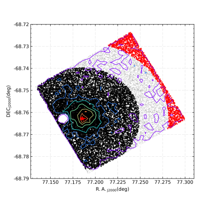
Next, we need to define the appropriate cluster and reference fields. To do so, we first inspected the radial surface brightness profile of NGC 1850. The spatial distribution and the number-density contours including all stars are shown in Fig. 1. The red pentagram indicates the cluster center, which corresponds to the highest two-dimensional number density. The resulting cluster center coordinates are $\alpha_{\rm J2000}=05^{\rm h}08^{\rm m}44.34^{\rm s}$, $\delta_{\rm J2000}=-68^{\circ}45^{\prime}45.60^{\prime\prime}$. These coordinates are in good agreement with the coordinates $\alpha_{\rm J2000}=05^{\rm h}08^{\rm m}44.79^{\rm s}$, $\delta_{\rm J2000}=-68^{\circ}45^{\prime}38.60^{\prime\prime}$ listed by the Strasbourg Astronomical Data Center’s SIMBAD database (http://simbad.u-strasbg.fr/simbad/). Black points concentrated around the red pentagram are cluster stars. We will analyze the behavior of the high-mass-ratio binaries (using their binary fractions, $f_{\rm bin}$) and blue-MS stars ($f_{\rm bMS}$) as a function of radius in this region (the extent of the region covered here was determined on the basis of the cluster’s surface brightness profile; see below for details).

At the distance of NGC 1850, $(m-M)_{0}=18.45$ mag (determined below and based on isochrone fitting), $1^{\prime\prime}$ corresponds to 0.24 pc. As we will see below, the cluster’s core radius, $r_{\rm c}$, is 2.76 pc and its radial profile disappears into the background noise at a radius of $\sim$83^′′ or 20 pc. We chose objects located at distances greater than 30 pc from the cluster center as reference stars (see the red points in Fig. 1), since those stars should be negligibly contaminated by cluster stars. They were used to statistically remove background stars from the adopted cluster region. Additionally, a small young star cluster (NGC 1850B) located to the southwest of our target cluster contains several young bright stars. To minimize any contamination by NGC 1850B, we removed objects located in an area with a radius of $8^{\prime\prime}$ centered on NGC 1850B. (The center coordinates of NGC 1850B were kept consistent with the location of the brightest star in the raw image, based on visual inspection, because the number density in this region is too low to determine the subcluster’s center coordinates on the basis of a density contour map. The adopted coordinates are $\alpha_{\rm J2000}=05^{\rm h}08^{\rm m}39.34^{\rm s}$, $\delta_{\rm J2000}=-68^{\circ}45^{\prime}45.80^{\prime\prime}$.)

Figure 1.— Spatial distributions of all stars (grey), stars within the adopted cluster region (black), reference field stars (red), and number density contours in the NGC 1850 field. The red pentagram indicates the cluster center at $\alpha_{\rm J2000}=05^{\rm h}08^{\rm m}44.34^{\rm s}$, $\delta_{\rm J2000}=-68^{\circ}45^{\prime}45.60^{\prime\prime}$. Objects located in the white circle to the left of the red pentagram were removed so as to minimize contamination by NGC 1850B stars.

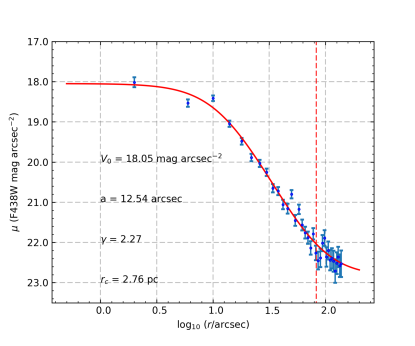
We used the cluster center to define annular rings at different radii and calculated the corresponding surface brightness profile. We followed the method introduced by Mackey & Gilmore (2003), adopting a $4^{\prime\prime}$ ring width. The resulting surface brightness profile is shown in Fig. 2. Since NGC 1850 is a YMC in the LMC, its surface brightness profile follows the canonical (Elson et al., 1987, EFF) profile,

$$\mu(r)=\mu_{0}(1+\frac{r^{2}}{a^{2}})^{-\gamma/2},$$ (1)

where $\mu_{0}$ is the central surface brightness. The EFF model’s core radius, $a$, and the power-law index $\gamma$ are linked to the core radius of the standard King model, $r_{\rm c}$, through

$$r_{\rm c}=a(2^{2/\gamma}-1)^{1/2}.$$ (2)

The parameters pertaining to the best-fitting EFF profile and the linked core radius of the King profile are also included in the bottom left-hand corner of Fig. 2. Our fit implies that the NGC 1850 core radius is $2.76\pm 0.12$ pc, which is consistent within one sigma with the value of $2.69^{+0.13}_{-0.17}$ pc derived by McLaughlin & van der Marel (2005, their Table 11). Through visual inspection, we determined that at a radius $R\sim 20$ pc ($\sim$83^′′; indicated by the vertical red dashed line in Fig. 2) the cluster’s surface brightness profile becomes indistinguishable from the field level. We therefore adopted this radius as that encompassing the typical cluster region (shown as the area containing the black points in Fig. 1). Note that in reality the surface brightness continues to decrease beyond the cluster region, however, so that the adopted value of 20 pc does not represent the full extent of the cluster. This is consistent with the conclusion of McLaughlin & van der Marel (2005), who derived a tidal radius for NGC 1850 of $\log(r_{\rm t}\mbox{ pc}^{-1})=2.16^{+0.09}_{-0.07}$.

Figure 2.— Surface brightness profile of NGC 1850. The red solid line is the best-fitting EFF profile. Error bars show Poissonian errors pertaining to each $4^{\prime\prime}$-wide annulus. The three parameters associated with the best-fitting EFF profile and the core radius from the linked King profile are shown in the bottom left-hand corner. The vertical red dashed line indicates the radius of the adopted cluster region.

3. Results

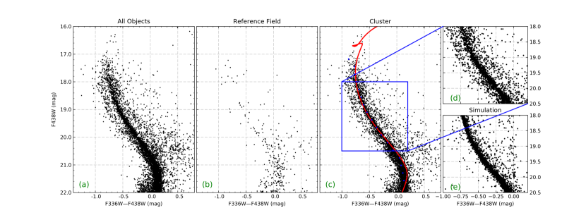
The CMDs of all stars in our observed field, the reference field stars, and the cluster stars are shown in Figs 3a, 3b, and 3c, respectively. We corrected for differential reddening by application of the method of Milone et al. (2012). The resulting differential reddening values across the cluster area ranged from $\vartriangle E(B-V)\sim-0.024$ mag to 0.023 mag, adopting the relative interstellar extinction coefficients $\frac{A_{\rm F336W}}{A_{V}}=1.66$ and $\frac{A_{\rm F438W}}{A_{V}}=1.33$ (Girardi et al., 2008). In Fig. 3c, we derived the basic cluster parameters using isochrone fitting. First, we divided stars with magnitudes in the range $17<m_{\rm F438W}<22$ mag into 30 bins. We then used Gaussian distributions to fit the color histograms in each bin. We chose the center color values of these Gaussian distributions as representative of our ridge line, shown as blue squares in Fig. 3c. We adjusted the parameters of the isochrones with reference to those blue squares. The best-fitting isochrone from the suite of PARSEC model isochrones (Bressan et al., 2012) yielded an age $\log(t\mbox{ yr}^{-1})=7.98^{+0.13}_{-0.15}$, a metallicity $Z=0.008$, a total extinction $A_{V}=0.3\pm 0.1$ mag, and a distance modulus $(m-M)_{0}=18.45^{+0.06}_{-0.08}$ mag. These parameters are mostly in good agreement with those derived by Bastian et al. (2016); these latter authors found a best-fitting age of 70–140 Myr, $Z=0.008$, and $(m-M)_{0}=18.35$ mag. Our best-fitting isochrone is shown as the red line in Fig. 3c. The cluster CMD exhibits a significant split in its MS in the magnitude range $19.0<m_{\rm F438W}<20.5$ mag. A zoomed-in view of the CMD focused on the split MS (indicated by the blue box in Fig. 3c) is shown in Fig. 3d. We also performed artificial-star experiments to make sure that the split MS is a real feature associated with NGC 1850. We first generated an artificial-star population containing 1000 data points with the same photometric properties as each isochrone point. We then reran DOLPHOT by adding the Fakestars option. The simulated CMD is shown in Fig. 3e.

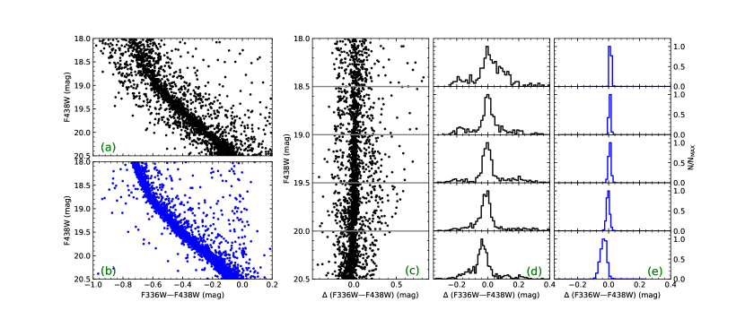
Figure 4 illustrates the process adopted to confirm the bimodal MS feature in NGC 1850. Figs 4a and 4b are equivalent to Figs 3d and 3e, respectively, showing zoomed-in CMDs of the observed and simulated stars in the region where we have detected the split MS. In Fig. 4c, we display the cluster’s observed stellar distribution in the $m_{\rm F438W}$ versus $\vartriangle(m_{\rm F336W}-m_{\rm F438W})$ diagram; the latter quantity corresponds to the color of the stars minus that of the best-fitting isochrone for the corresponding F438W magnitude. Comparing the observed $\vartriangle(m_{\rm F336W}-m_{\rm F438W})$ distribution (Fig. 4d) with the corresponding simulated distribution (Fig. 4e), it is clear that the observed histograms exhibit a significant double peak in brighter magnitude bins, which merges into a single peak at fainter magnitudes, corresponding to the disappearance of the bimodal MS. However, the simulated histograms always shows a single-peaked distribution; the larger photometric errors on the faint end broaden the width of the peak. We thus conclude that the split MS is intrinsic to the cluster and cannot be caused by photometric errors alone.

Figure 3.— CMDs of (a) all stars in our observed field, (b) reference field stars (selected in Section 2), and (c) cluster stars. The ridge line defined by the cluster stars in the range $17<m_{\rm F438W}<22$ mag is shown by the blue squares. The red line represents the best-fitting isochrone, with $\log(t\mbox{ yr}^{-1})=7.98$, $Z=0.008$, $A_{V}=0.3$ mag, and $(m-M)_{0}=18.45$ mag; (d) zoomed-in view focused on the split MS region (indicated by the blue box in panel c); (e) CMD of the artificial stars.

Figure 4.— Illustration showing that a bimodal MS is an intrinsic feature of NGC 1850, which cannot have been caused by photometric errors alone. The CMDs of the observed stars (black dots) and the simulated stars (blue dots) are shown in panels (a) and (b), respectively. Panel (c) shows the $m_{\rm F438W}$ versus $\vartriangle(m_{\rm F336W}-m_{\rm F438W})$ CMD based on observed data. Panels (d) and (e) show the distribution of the $\vartriangle(m_{\rm F336W}-m_{\rm F438W})$ color in five magnitude intervals for the observed and simulated stars, respectively.

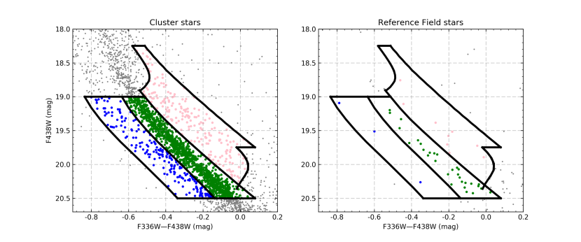
We are interested in the clearly split MS feature located at $19.0<m_{\rm F438W}<20.5$ mag. Therefore, we applied a method similar to that adopted by Milone et al. (2017) to divide those stars into blue-MS, red-MS, and high-mass-ratio binary stellar samples. A zoomed-in view of the CMD and the areas adopted for the blue-MS stars, red-MS stars, and high-mass-ratio binaries are shown as blue, green, and pink points in the left-hand panel of Fig. 5. The sample boundaries were defined as follows. First, we chose the best-fitting isochrone for the magnitude range $19.0<m_{\rm F438W}<20.5$ mag. From the PARSEC output data, i.e., the initial mass and the F336W and F438W magnitudes, we can then interpolate and derive the magnitude and color for any binary system for a given mass ratio $q=M_{1}/M_{2}$, where $M_{1}$ and $M_{2}$ are the masses of the binary system’s primary and secondary components, respectively. Thus, we obtained MS–MS binary sequences for different mass ratios; for $q=1$, the MS–MS binary sequence represents a simple upward shift of the single-star isochrone by 0.752 mag (see Elson et al., 1998, their Fig. 3).

The red and blue boundaries of the red MS are defined by moving the best-fitting isochrone by an additional $1.5\sigma$ given by the photometric errors in both the color and magnitude directions. Note that our data are characterized by small photometric uncertainties, since we adopted only high-quality data. We also note that the DOLPHOT output uncertainties are rather too small; if we would use the DOLPHOT uncertainties directly, the fiducial sequence would not be included in the red-MS region. Therefore, we adopted the standard deviations of the magnitudes in both filters from our artificial-star tests (Fig. 3e) as our photometric uncertainties, which include the systematic errors. This method is similar to that adopted by Milone et al. (2017). The latter authors shifted the ridge line of the cluster’s red MS by $2\sigma_{\rm c}$ toward the blue, where $\sigma_{\rm c}$ is the uncertainty in color.

The bright and faint boundaries of the blue and red MSs were set at $m_{\rm F438W}=19.0$ mag and $m_{\rm F438W}=20.5$ mag, respectively. The red boundary of the high-mass-ratio binaries was defined by shifting the sequence of equal-mass binaries to the red by $1.5\sigma$, where $\sigma$ is the uncertainty in the color. Note that the pink points are mostly located above the $q=0.55$ MS–MS binary sequence, hence our reference to ‘high-mass-ratio’ binaries. The top and bottom boundaries of the pink region were obtained through interpolation, starting from the different mass ratios corresponding to the equivalent points on the single-star isochrone at $m_{\rm F438W}=19.0$ mag and $m_{\rm F438W}=20.5$ mag, respectively. The blue boundary of the blue MS was drawn arbitrarily to make sure that we include the majority of objects in that regime. The right-hand panel of Fig. 5 shows the same boundaries for the reference field stars. Our final sample of blue-MS stars includes 194 objects; our catalog also includes 1176 red-MS stars and 210 high-mass-ratio binaries in the cluster region, as well as three blue-MS stars, 30 red-MS stars, and 10 high-mass-ratio binaries in the reference field.

Figure 5.— Zoomed views of the CMD region of interest exhibiting split MSs. The left-hand panel shows the distribution of blue-MS stars (blue), red-MS stars (green), and high-mass-ratio binaries (pink) in the cluster region. The right-hand panel is the same but for the reference field.

We calculated the population ratio of blue-MS stars and high-mass-ratio binaries with respect to the total number of stars in the three regions for different radii:

$$f_{\rm bMS}(r)=\frac{(N_{\rm bMS}(r)-A(r)n_{\rm bMS})\times\frac{P({\rm in})_{\rm bMS}(r)}{P({\rm out})_{\rm bMS}(r)}}{N_{\rm bMS}(r)+N_{\rm rMS}(r)+N_{\rm bin}(r)};$$ (3)

$$f_{\rm bin}(r)=\frac{(N_{\rm bin}(r)-A(r)n_{\rm bin})\times\frac{P({\rm in})_{\rm bin}(r)}{P({\rm out})_{\rm bin}(r)}}{N_{\rm bMS}(r)+N_{\rm rMS}(r)+N_{\rm bin}(r)}.$$ (4)

Here, $N_{\rm bMS}$, $N_{\rm rMS}$, and $N_{\rm bin}$, are the numbers of blue-MS stars, red-MS stars, and high-mass-ratio binaries in the different annular rings, respectively; $n_{\rm bMS}$ and $n_{\rm bin}$ are the corresponding numbers for stars located in the same regions in the CMD of the reference field. $A(r)$ is the correction factor for the areal difference between the ring and the reference field. This value is defined by means of Monte Carlo simulations. (In detail, we generated one million uniformly distributed data points in the right ascension–declination plane, counting the numbers of points located in annular rings and the reference field, i.e, $A(r)=\frac{N_{\rm ring}(r)}{N_{\rm reference}}$.)

$\frac{P({\rm in})(r)}{P({\rm out})(r)}$ is a photometric correction factor. Single stars in the cluster center may appear like binaries because of the crowded environment in the cluster core and because of stellar blends. Thus, a blue-MS star can be pushed into the CMD region of the red-MS stars, while a red-MS star can be pushed into the region containing the cluster’s binaries. It is therefore necessary to correct for the number difference caused by the process of obtaining our photometry. To do so, we generated more than 200,000 artificial stars, inserted them into the raw image, and then measured them in exactly the same way as the real stars. Specifically, we first generated 100 artificial stars located in the black-bordered region of Fig. 5 with uniform color–magnitude and spatial distributions. Next, we reran DOLPHOT with the added Fakestars option, thus allowing us to assess the differences between the input and output photometry. We repeated this process more than one thousand times for each chip to reduce the effects of statistical fluctuations. We generated 100 artificial stars each time so as to avoid the situation where artificial stars would significantly increase the crowding of our images. Finally, we calculated the number ratio of the input and output artificial stellar samples using the same approach as that introduced to deal with Fig. 5, thus resulting in the photometric correction factor.

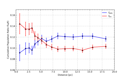
In this paper, we are only concerned with the number-fraction profiles of the blue-MS stars and high-mass-ratio binaries. We divided all colored stars in Fig. 5 into 15 different annular rings, imposing the condition that these annular rings contain almost the same numbers of colored stars. The cumulative number-fraction profiles are shown in Fig. 6. The number fractions of the high-mass-ratio binaries, $f_{\rm bin}(\leq R)$, and of the blue-MS stars, $f_{\rm bMS}(\leq R)$, show a significant negative correlation. The Pearson coefficient pertaining to the cumulative population is $-0.97$, which satisfies the condition that “if the absolute Pearson coefficient exceeds 0.7, the correlation between two data sequences is significant.” Figure 6 thus reveals a potential correlation between both stellar samples, which we will discuss in the next section.

Additionally, radially dependent photometric errors could also introduce spurious trends. The photometric errors may be large in the cluster center and small in the outskirts because of crowding in the cluster core. From the CMD, we infer that more intrinsic red-MS stars (blue-MS stars, high-mass-ratio binaries) would move to the blue-MS stars region or high-mass-ratio binaries in the cluster center, while stars would remain in their original region in the cluster’s periphery. This means that our photometry procedure cannot fully reproduce the input distribution but introduces a small, non-real gradient. We conducted artificial-star experiments to check the importance of this effect on our observed number fraction profiles. In particular, we generated single fake stars along the ridge lines of the observed blue- and red-MSs. We also generated 30% binaries for each single-star sample with a flat mass-ratio distribution. The spatial coordinates of all artificial stars follow the same radial distribution. We obtained PSF photometry for the artificial stars using DOLPHOT. We used the same approach as employed for the real stars to reduce the simulated data and derived the radial distributions of blue-MS stars and binaries. The measured number fractions of blue-MS stars are significantly higher than the input values in the inner rings, and they decrease in the outer rings. However, the measured number fraction of binaries remains almost the same as the input values in all rings. In other words, the simulated radial distribution is such that the artificial blue-MS is more centrally concentrated than the red-MS population. Therefore, we come to the conclusion that the blue-MS fraction is overestimated, while radially dependent photometric errors would not change the main result.

Figure 6.— Cumulative population of blue MS stars (blue line) and high-mass-ratio binaries (red line) with respect to the total numbers of sample stars at different radii. The vertical error bars represent Poissonian errors. Both profiles are strongly anti-correlated for radii within a few parsecs from the cluster center.

4. Discussion

The origin of the blue MS remains a puzzle. D’Antona et al. (2015) interpreted the CMD of the YMC NGC 1856 as a superposition of two populations, i.e., one-third of the total number of stars is composed of slowly/non-rotating stars and two-thirds of rapidly rotating stars. A key problem arising from this scenario is that rapid rotation is a common feature of B–A-type stars, so one should then wonder why there are so many slowly/non-rotating stars. One possibility regarding the origin of the slowly/non-rotating stars is that most blue-MS stars might hide a binary component, where the tidal interaction between the binary components is held responsible for slowing down the rotation rate (D’Antona et al., 2017). If this suggestion is correct and also holds for NGC 1850, there might be a link between the spatial distributions of the blue-MS stars and the high-mass-ratio binaries. Our results thus offer some hints as regards this possible correlation.

The origin of the apparent anti-correlation between the radial number-fraction profiles of the blue-MS stars and the high-mass-ratio binaries is not clear. Li et al. (2013) showed the opposite trend for the F-type binaries’ radial profiles in both NGC 1805 and NGC 1818. They concluded that this opposite trend could have been caused by the clusters’ different dynamical ages. NGC 1805 is dominated by dynamical mass segregation while the evolution of NGC 1818 is still dominated by binary disruption. Their calculations confirmed that NGC 1805 is dynamically older than NGC 1818. Using $N$-body simulations, Geller et al. (2013) showed that the radial distribution of binary systems in rich star clusters can evolve from a decreasing trend toward a cluster’s core to an increasing trend, depending on the dynamical timescale. A cluster’s dynamical age is a key parameter of importance for the shape of a stellar sample’s radial profile.

In addition, it seems that most of the binaries populating the blue MS are low-mass-ratio binaries ($q<0.55$), which we cannot easily distinguish from single stars, given the prevailing photometric uncertainties. They are likely still in their dynamical disruption phase, while the high-mass-ratio binaries are more segregated. To confirm the dynamical phase governing the blue-MS stars and the high-mass-ratio binaries in NGC 1850, we calculated the half-mass relaxation times for both samples (Meylan, 1987),

$$t_{r,{\rm h}}=(8.92\times 10^{5})\frac{M_{\rm tot}^{1/2}}{m}\frac{R_{\rm h}^{3/2}}{\log(0.4M_{\rm tot}/m)}\mbox{ yr}.$$ (5)

The total mass of NGC 1850 was calculated using the relation between the initial stellar masses and magnitudes in the F438W filter provided by the best-fitting PARSEC isochrone data table. The total luminous mass of NGC 1850 based on our F438W observations is $\log M_{\rm tot}/M_{\odot}=4.360\pm 0.001$ and the half-mass radius $R_{\rm h}=9.239^{+0.009}_{-0.017}$ pc. We also estimated the mass of NGC 1850 based on the canonical initial mass function (Kroupa, 2001), $\log M_{\rm tot}/M_{\odot}=4.64^{+0.09}_{-0.07}$. Correnti et al. (2017) derived $\log M_{\rm tot}/M_{\odot}=4.86\pm 0.10$ and $\log M_{\rm tot}/M_{\odot}=4.62\pm 0.10$ based on Salpeter (1955) and Chabrier (2003) initial mass functions, respectively. The luminous mass estimate we obtained here is the smallest value. The typical masses of our stellar samples are also required to calculate the half-mass relaxation time. Since binaries are completely unresolved in the LMC, binary systems will look like single point-like sources. With $m_{1}$, $m_{2}$, $F_{1}$, and $F_{2}$ defined as the magnitudes and fluxes of primary and secondary stars in a binary system, the combined magnitude of the binary system is

$$m_{\rm bin}=m_{1}-2.5\log(1+\frac{F_{2}}{F_{1}}).$$ (6)

Since the observed fluxes are related to the underlying stellar masses, the combined magnitudes of MS–MS binary systems depend on the relevant mass ratios, $q=M_{2}/M_{1}$. We can calculate the MS–MS binary sequences for different mass ratios and the curve defining the change in luminosity for a given initial mass (Elson et al., 1998). MS–MS binary sequences and luminosity change curves compose a grid covering the CMD. In this grid, one object corresponds to one set of coordinates, $(q,M_{\rm ini})$. The mass of photometric MS–MS binary systems can be obtained by optimizing the combination of $q$ and $M_{\rm ini}$. We thus calculated the average mass of our high-mass-ratio binaries, i.e. $4.52M_{\odot}$. The average mass of blue-MS stars is $2.52M_{\odot}$, which was calculated through interpolation (i.e, we can derive the mass of a blue-MS star with any magnitude through the relationship between the initial mass and the F438W magnitudes of the best-fitting isochrone data).

Our aim of estimating the half-mass relaxation time here is to compare the dynamical stages of our stellar samples, not to determine precise values. Our rough estimates of the half-mass relaxation times of the high-mass-ratio binaries and the cluster’s blue-MS stars are 253.7 Myr and 422.6 Myr, respectively, while the respective core relaxation times are 38.3 Myr and 63.8 Myr. The dynamical timescale is always longer for the blue-MS stars than for the high-mass-ratio binaries. This confirms the assumption that the blue-MS stars are dynamically younger than the high-mass-ratio binaries. This then supports the suggestion that the blue-MS stars are low-mass-ratio binaries, which have lower binding energies than high-mass-ratio binary systems, because the binding energy of a binary system is directly proportional to the masses of its stellar components ($E\varpropto qM^{2}$), on average. Generally speaking, after suffering numerous encounters in a stellar system, soft binaries become softer, while hard binaries become harder (Heggie, 1975). That is indeed the reason why the high-mass-ratio binaries in NGC 1850 are more segregated than their low-mass-ratio counterparts. However, ideally we prefer a shorter half-mass relaxation timescale for high-mass-ratio binaries than the cluster age, while we would expect the equivalent timescale for blue-MS stars to be longer than the cluster age. Of course, this discussion assumes that the cluster is located in an isolated environment. We note, however, that NGC 1850 is located at the northern end of the LMC’s bar structure. In addition, the young cluster NGC 1850B is located to the west of NGC 1850, within about $30^{\prime\prime}$. Both of those structures may contribute to accelerating the cluster’s dynamical evolution, so the half-mass relaxation times estimated above are upper limits.

We tentatively suggest that dynamical mass exchange of binaries may link the low- and high-mass-ratio binaries, thus producing a radial anti-correlation between them. There are two channels by which a binary system can be hardened through interactions with single stars. First, extraction of internal energy from the binary by a single star would make a binary system more strongly bound. This process is important when the average mass of the surrounding stars and the local stellar number density are not very high, e.g., in the outer regions of star clusters. Second, a low-mass-ratio binary system can transfer internal energy to its surroundings through mass exchange. The lower-mass component in the binary system is thereby replaced by a higher-mass field star. As a result, it becomes a high-mass-ratio binary system. This process is favored when the masses of the surrounding stars are higher than the mass of one component of a binary system, e.g., in the mass-segregated core region of a star cluster.

The second channel for binary hardening is actually a combination of the destruction of low-mass-ratio binaries and the production of high-mass-ratio binaries, thus causing mutual exclusion. Because all binaries studied here have mass ratios $q\geq 0.55$, if the blue-MS stars are indeed low-mass-ratio binaries and if they are still affected by mass exchange, their radial number-fraction profile may be anti-correlated with the high-mass-ratio binaries. In addition, because mass exchange favors dense cluster core regions, the anti-correlation between the number fraction of low- and high-mass-ratio binaries should be more significant in a cluster’s central region, which is indeed observed in NGC 1850 (Fig. 6).

Our proposed scenario agrees to a large extent with the stellar rotation models. However, here we suggest that the blue-MS may be populated by low-mass-ratio binaries, whereas D’Antona et al. (2017) interpreted blue-MS stars as slowly rotating stars following a period of ‘braking.’ Indeed, it is well-known that rapid rotation is a common feature among stars, and tidal torques in binary systems can slow down the rotation rates significantly. There is no direct observational evidence showing that low-mass-ratio binaries are more likely to be affected by tidal interactions than high-mass-ratio binaries. For the same gravitational environment and conditions, low-mass-ratio binaries preferentially have smaller separations. Thus, they can survive just as well as high-mass-ratio binaries, since the binding energy $E\varpropto\frac{qM^{2}}{r}$. The smaller the binary system’s separation is, the stronger the effects of tidal synchronization will be. Therefore, the rotation rates of the primary stars of surviving low-mass-ratio binaries are more easily affected by tidal synchronization. As a result, we would observe bluer primary stars on the whole, because of the decrease in rotation rates. In addition, if tidal synchronization slows down the primary stars in unresolved systems, high-mass companions would make stars look redder and brighter, and high-mass-ratio binaries would not be found on the blue-MS. Note that, at the present time, this is merely a speculative conclusion.

However, Milone et al. (2017) studied the same behavior for another YMC, NGC 1866. They did not detect any evidence of such an anti-correlation between the radial number-fraction profiles of the blue-MS stars and the cluster’s high-mass-ratio binaries. On the contrary, their result seems to support that the number-fraction profiles of the blue-MS stars and the high-mass-ratio binaries are positively correlated (their Fig. 9). The half-light relaxation times of NGC 1866 and NGC 1850 are $\log t_{r,{\rm h}}=9.55_{-0.08}^{+0.06}$ yr and $\log t_{r,{\rm h}}=9.58_{-0.10}^{+0.05}$ yr, respectively (McLaughlin & van der Marel, 2005). The best-fitting isochrone age for NGC 1866 varies from 140 Myr to 220 Myr. Comparing the cluster ages and half-mass relaxation times of these two YMCs, we come to the conclusion that NGC 1866 is dynamically much older than NGC 1850, which again supports our proposed scenario. In summary, NGC 1866 is dynamically more evolved than NGC 1850, and the pool of low-mass-ratio systems may already have evolved in the core of NGC 1866. In turn, this has resulted in the observed positive correlation between this cluster’s blue-MS and high-mass-ratio radial profiles.

Because measuring the mass ratio of an individual binary system located in a dense LMC cluster is not possible at the present time, our proposed scenario is currently only a theoretical possibility. Similar studies for other analogous YMCs will help us to better understand the potential physics governing these blue-MS stars.

5. Summary

In this paper, we have studied the radial number-fraction profiles of the blue-MS stars and the high-mass-ratio binaries in the YMC NGC 1850. We aimed to examine if the observed blue-MS stars are binary-related objects, as suggested by D’Antona et al. (2015, 2017). Our analysis reveals that (1) the blue-MS stars show an inverse radial segregation, while the high-mass-ratio binaries are more segregated than the cluster’s bulk stellar population; and (2) the radial number-fraction profiles of the blue-MS stars and the high-mass-ratio binaries are strongly anti-correlated in the cluster core.

We suggest that most blue-MS stars may be low-mass-ratio binaries. They might still be experiencing dynamical disruption. Mass exchange between these low-mass-ratio binaries and the surrounding population of massive stars is likely taking place at the present time, which causes an increase in their mass ratio. This process is responsible for turning low-mass-ratio binaries into high-mass-ratio systems, thus producing an inverse correlation between both types of binary system. However, because of the absence of definitive evidence, whether or not this scenario is correct remains an open question.

References

- Bastian & de Mink (2009) Bastian, N., & de Mink, S. E. 2009, MNRAS, 398, L11
- Bastian et al. (2016) Bastian, N., Niederhofer, F., Kozhurina-Platais, V., et al. 2016, MNRAS, 460, L20
- Brandt & Huang (2015) Brandt, T. D., & Huang, C. X. 2015, ApJ, 807, 24
- Bressan et al. (2012) Bressan, A., Marigo, P., Girardi, L., et al. 2012, MNRAS, 427, 127
- Chabrier (2003) Chabrier, G. 2003, PASP, 115, 763
- Correnti et al. (2017) Correnti, M., Goudfrooij, P., Bellini, A., Kalirai, J. S., & Puzia, T. H. 2017, MNRAS, 467, 3628
- D’Antona et al. (2015) D’Antona, F., Di Criscienzo, M., Decressin, T., et al. 2015, MNRAS, 453, 2637
- D’Antona et al. (2017) D’Antona, F., Milone, A. P., Tailo, M., et al. 2017, Nature Astronomy, 1, 0186
- de Grijs et al. (2013) de Grijs, R., Li, C., Zheng, Y., et al. 2013, ApJ, 765, 4
- Elson et al. (1987) Elson, R. A. W., Fall, S. M., & Freeman, K. C. 1987, ApJ, 323, 54
- Elson et al. (1998) Elson, R. A. W., Sigurdsson, S., Davies, M., Hurley, J., & Gilmore, G. 1998, MNRAS, 300, 857
- Geller et al. (2013) Geller, A. M., de Grijs, R., Li, C., & Hurley, J. R. 2013, ApJ, 779, 30
- Geller et al. (2015) —. 2015, ApJ, 805, 11
- Girardi et al. (2008) Girardi, L., Dalcanton, J., Williams, B., et al. 2008, PASP, 120, 583
- Girardi et al. (2013) Girardi, L., Goudfrooij, P., Kalirai, J. S., et al. 2013, MNRAS, 431, 3501
- Goudfrooij et al. (2015) Goudfrooij, P., Girardi, L., Rosenfield, P., et al. 2015, MNRAS, 450, 1693
- Goudfrooij et al. (2011) Goudfrooij, P., Puzia, T. H., Kozhurina-Platais, V., & Chandar, R. 2011, ApJ, 737, 3
- Heggie (1975) Heggie, D. C. 1975, MNRAS, 173, 729
- Kroupa (2001) Kroupa, P. 2001, MNRAS, 322, 231
- Li et al. (2016) Li, C., de Grijs, R., Bastian, N., et al. 2016, MNRAS, 461, 3212
- Li et al. (2013) Li, C., de Grijs, R., & Deng, L. 2013, MNRAS, 436, 1497
- Li et al. (2017) Li, C., de Grijs, R., Deng, L., & Milone, A. P. 2017, ApJ, 834, 156
- Mackey & Gilmore (2003) Mackey, A. D., & Gilmore, G. F. 2003, MNRAS, 338, 85
- McLaughlin & van der Marel (2005) McLaughlin, D. E., & van der Marel, R. P. 2005, ApJS, 161, 304
- Meylan (1987) Meylan, G. 1987, A&A, 184, 144
- Milone et al. (2009) Milone, A. P., Bedin, L. R., Piotto, G., & Anderson, J. 2009, A&A, 497, 755
- Milone et al. (2016) Milone, A. P., Marino, A. F., D’Antona, F., et al. 2016, MNRAS, 458, 4368
- Milone et al. (2012) Milone, A. P., Piotto, G., Bedin, L. R., et al. 2012, A&A, 540, A16
- Milone et al. (2015) Milone, A. P., Bedin, L. R., Piotto, G., et al. 2015, MNRAS, 450, 3750
- Milone et al. (2017) Milone, A. P., Marino, A. F., D’Antona, F., et al. 2017, MNRAS, 465, 4363
- Piatti & Cole (2017) Piatti, A. E., & Cole, A. 2017, MNRAS, 470, L77
- Salpeter (1955) Salpeter, E. E. 1955, ApJ, 121, 161
- Wu et al. (2016) Wu, X., Li, C., de Grijs, R., & Deng, L. 2016, ApJ, 826, L14
- Yang et al. (2011) Yang, W., Meng, X., Bi, S., et al. 2011, ApJ, 731, L37