Offline Object Extraction from
Dynamic Occupancy Grid Map Sequences^⋆ 

Abstract

A dynamic occupancy grid map (DOGMa) allows a fast, robust, and complete environment representation for automated vehicles. Dynamic objects in a DOGMa, however, are commonly represented as independent cells while modeled objects with shape and pose are favorable. The evaluation of algorithms for object extraction or the training and validation of learning algorithms rely on labeled ground truth data. Manually annotating objects in a DOGMa to obtain ground truth data is a time consuming and expensive process. Additionally the quality of labeled data depend strongly on the variation of filtered input data. The presented work introduces an automatic labeling process, where a full sequence is used to extract the best possible object pose and shape in terms of temporal consistency. A two direction temporal search is executed to trace single objects over a sequence, where the best estimate of its extent and pose is refined in every time step. Furthermore, the presented algorithm only uses statistical constraints of the cell clusters for the object extraction instead of fixed heuristic parameters. Experimental results show a well-performing automatic labeling algorithm with real sensor data even at challenging scenarios.

I Introduction

For automated driving or modern driver assistant systems, a detection of the vehicle surrounding is essential. For that reason, more and more sensors are mounted on the vehicle to generate dense and precise measurements of the environment. A well-studied topic to detect and track external dynamic objects in the environment is using temporal filtering algorithms [1]. These object-model-based representations use Bayesian filtering techniques and manage to suppress clutter and false alarms, and are able to track multiple objects at once [2, 3]. Despite the impressive success, object tracking in crowded urban shared space scenarios is still an tough challenge. Using occupancy grid maps is a complementing alternative to process sensor measurements and represent the complete environment object-model-free [4]. Therefore, the local environment is separated in grid cells, where the state of each cell is an estimation of the probabilities for occupied and free. The extension to a dynamic occupancy grid map (DOGMa) [5, 6, 7] enables the estimation of dynamics in any cell. A main advantage of grid maps is the simple accumulation of sensor measurements from different sensors at different time steps. Each cell is processed independently without any assumptions of object shapes, movements or types. Consequently, a detection of the entire environment including all traffic participants is possible.

Due to the independence of cells, there is no information of the associated object generating these measurements. However, for autonomous applications, e.g. behavior planning [8], full knowledge of the single object state is favorable. To achieve this, a major challenge is to extract objects from the grid map by associating cells to objects and represent them with spatial and dynamic information.

Figure 1: Overlay of the DOGMa and Google Maps in Ulm inner city with extracted objects as orange rectangles after the full sequence is processed.

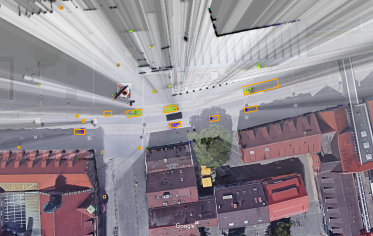
In this work we present an offline approach to extract dynamic objects from a DOGMa. Therefore, the presented algorithm uses acausal information from the future and past to generate a ground truth object state to any time. Starting from a moment where an object is clearly visible, it can be traced forward and backward in time, while the correct shape, pose and trajectory is refined via best fit on the entire sequence. Due to this algorithm, even challenging separations of objects moving next to each other and precise spatial information of occluded or barely visible objects are possible. An example of the algorithm’s result is shown in Figure 1. Therefore, an overlay of the satellite image from Google Maps and a DOGMA generated with Lidar sensors at an urban area is depicted. Rectangles represent the extracted objects pose and shape, as width and length, after the presented two directional search. It is clearly visible that even objects with only a few number of cells hold the exact estimation of the shape. Additionally the algorithm is designed to require almost no heuristic parameters and uses statistical constraints instead. The main goal of the algorithm’s result is intended to serve as ground truth to evaluate object extraction algorithms, e.g. based on clustering techniques like DBSCAN [9], or as labels for learning techniques on grid maps what gains interest in current research [10, 11].

The remaining paper is structured as follows: A short insight of related work for objects extraction of grid maps is reviewed in Section II. An implementation of the DOGMa and a prepossessing of the algorithm is described in Section III. The object extraction algorithm with its detailed description is given in Section IV and Section V. Resulting extracted objects from the presented algorithm and limitations are shown in Section VI followed by conclusions given in Section VII.

II Related Work

A common approach to extract objects from the occupancy grid map is based on a combination of multi-object tracking algorithms. In [12] a fusion approach is presented where a Kalman filter processes the cell states to improve the object tracking estimate. Therefore, an association between the grid map cells and the current track is necessary, what is realized with a grouping algorithm using a distance criterion. The approach by Jungnickel [13] presents an object tracking based only on occupancy grid maps. A particle filter tracks a dynamic cell cluster what represents an arbitrary object shape. For state estimation the DBSCAN algorithm clusters dynamic cells and to sets up new object tracks. Sch tz et al. [14] perform an extended object tracking [15] using a local grid to estimate the objects shape. Here, the DBSCAN algorithm is also used to cluster the measurements by defining a range parameter $\epsilon$ and minimum number of cells $k_{min}$. Recently published approaches by [16, 17] seem very promising for detecting objects and tracking the pose and shape of objects. However, setting up new objects requires well separable clusters and small uncertainties in the cells. Additionally, heuristic parameter tuning is commonly required and strongly dependent on the density in the scene. Summarized, all online object tracking approaches suffer from engineered feature selections and parameter adjustments. In [10, 11] CNNs were trained on DOGMa input to detect and predict objects, while the objects are still represented as single independent cells, rather than clusters or boxes. Nevertheless, hours of training data, that commonly is labeled manually, is required to use neural networks efficiently. This procedure is expensive and time intensive for a huge amount of data. Due to offline processing, it is possible to automatically label ground truth data by using a two direction temporal search. An object detection algorithm, i.e. detecting rotated bounding boxes in a DOGMa, trained with the result presented in this work was published in [18].

III Preprocessing

The DOGMa is an implementation of [6], where cells $c$ discretize the local environment as spatial grid at the Universal Transverse Mercator (UTM) coordinates $(\mathrm{E},\mathrm{N})$. The spatial grid provides cells in $\mathbb{R}^{W\times H}$ with width $W$ and height $H$ pointing east and north, respectively. A particle filter estimates the static and dynamic state per cell. A cell comprises $\Omega_{c}=\left\{M_{\mathrm{O}},M_{\mathrm{F}},v_{\mathrm{E}},v_{\mathrm{N}},\sigma^{2}_{v_{\mathrm{E}}},\sigma^{2}_{v_{\mathrm{N}}},\sigma^{2}_{v_{\mathrm{E}},v_{\mathrm{N}}}\right\}$ with the Dempster Shafer [19] masses for occupancy $M_{\mathrm{O}}\in\left[0,1\right]$ and free space $M_{\mathrm{F}}\in\left[0,1\right]$. Furthermore, a velocity in east $v_{\mathrm{E}}$ and north $v_{\mathrm{N}}$ direction with appropriate (co-)variances $\left\{\sigma^{2}_{v_{\mathrm{E}}},\sigma^{2}_{v_{\mathrm{N}}},\sigma^{2}_{v_{\mathrm{E}},v_{\mathrm{N}}}\right\}$ is estimated. The grid map cell states $\Omega_{c}(t)$ are given at any time step $t$ of the sequence. The occupancy probability of a cell is calculated by $P_{\mathrm{O}}=0.5\cdot M_{\mathrm{O}}+0.5\cdot(1-M_{\mathrm{F}})$.

The input data for the algorithm is the ego motion aligned grid map sequence (EMAGS) which is a stack of temporal excerpts from a DOGMa sequence. It is generated by aligning snapshots from the DOGMa according to the ego motion of the perceiving vehicle, to generate a persistent map along the sequence. Therefore, even the ego vehicle generates a moving object in the EMAGS, but static objects stay on the same position over time. Additionally, this implies that every slice in the EMAGS may have other spatial boundaries, depending on the ego motion. The EMAGS is illustrated in Fig. 2, where

Figure 2: Illustrated EMAGS (top) where each slice is another time step, stacked on top of the previous time step. Static objects, such as walls or pillars, can be seen as vertical objects. Moving objects appear similar to staircases. The red vertical line (top) and curve (bottom) illustrate the occupancy of a single cell traversed by an object.

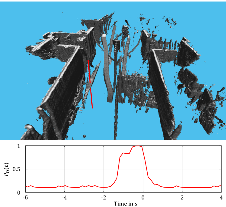
static objects can be seen as vertical objects, while moving objects appear similar to a staircase. In the image, a red line is drawn along the time axis with constant cell coordinates. The according curve $P_{\mathrm{O}}(t)$ is given in the plot in Fig. 2.

Algorithm 1 describes the main preprocessing steps. It aims at reasonable initialization points to start object extraction and spatial borders ideally representing object silhouette bounds.

Algorithm 1 Preprocessing of the EMAGS

0:  EMAGS

0:  Border mask and list of initialization points

  Spatial and temporal smoothing

  for each time step do

     Extract edges

     Generate possible object border lines

     Calculate center points

  end for

  return  border mask and initialization points

The EMAGS is first smoothed with a $3$D Gaussian in $P_{\mathrm{O}}(\mathrm{E},\mathrm{N},t)$. The first and second derivative is calculated along all $3$ dimensions to obtain points of inflections spatially and temporally. Similar to edge detection the found points represent sinks and raises of $P_{\mathrm{O}}(\mathrm{E},\mathrm{N},t)$. We consider the found points as border mask in spatial domain. In time domain, for each cell time steps $P_{\mathrm{O}}(t)$ within a raise and a slope, as illustrated by the plot in Fig. 2, are considered as traversed by a moving object. We use cluster centers of these points as initialization points for the extraction algorithm explained in the following sections. One slice, i.e. time step, of the preprocessing result is shown in Fig. 3 including a zoomed view showing initialization points in detail. The border mask is plotted in blue, where each marked point is part of the border of a possible object. The green points are the initialization points marking an inner point of a possible object. It is possible for an object to have multiple or no initialization points in a specific time step, as the preprocessing is a coarse first evaluation.

Figure 3: One time step of the preprocessed data is shown, referring to one slice from the EMAGS. The occupancy information is used as background, where black means occupied and white means not occupied. The border mask is shown in blue lines and the calculated initialization points are plotted in green. A zoomed excerpt is integrated in the bottom left, including two possible objects. One is marked with a single initialization point, the other with multiple. A third occupied area is seen, but it does not move over time, so it is not marked as possible object.

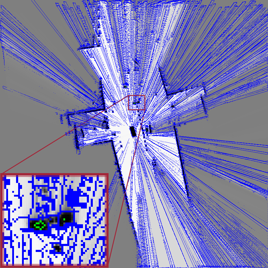
However, every object that has a clear appearance at least once in the sequence will be marked with an initialization point in that time step. This data is the output of preprocessing and will be used in the main algorithm to extract actual objects with their correct shapes. At this point, there is no temporal connection established between the initialization points, as it is not clear if every initialization point marks an actual object.

IV Algorithm Overview

Figure 4: Overview over the introduced algorithm. First and third row show the prediction step including the predicted object silhouette as green rectangle and the calculated starting points for the next component search in red crosses. The second and fourth row show the result of the component search and the object pose estimation. The pink and red marked cells are the first and the reduced blob. The object’s reference point is marked as blue cross. The beige and orange rectangles are the blob bounding box and the object bounding box, respectively.

The present algorithm automatically generates object labels in the EMAGS to enable their use as ground truth or comparison data. Every object is traced through the considered sequence using the best fitting of length and width, which is obtained over multiple time steps. The result is an automatically labeled EMAGS, where ideally every occurring object has its correct dimension and position in every time step, even if the true dimensions are only observed in few time steps. As the algorithm consists of multiple complex steps, this section gives an overview over the whole procedure, while the individual parts are explained separately in Sec. V.

Algorithm 2 Overview

0:  EMAGS

0:  labeled EMAGS

  preprocess EMAGS to calculate initialization points and border mask

  while get initialization point do

     Object initialization: connected component, polygon, velocity profile

     Start temporal search

     for forward step, backward step do

        while in sequence and object plausible do

           Object silhouette prediction

           Get connected component search starting points

           Extract connected component: first blob

           Blob reduction via outlier removal

           Calculate velocity profile

           Object plausibility check

           Construct blob polygon and get reference point

           Update object width and length estimation

           Construct object polygon

        end while

        Start backward step with best object estimates from forward step

     end for

     Delete initialization points covered by extracted object

     Object and trajectory consistency validation

     Orientation correction for standing objects

     (optional) Temporal trajectory smoothing

     Write object to result

  end while

  return  labeled EMAGS

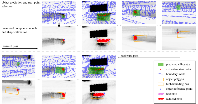
The pseudocode in Algorithm 2 introduces the idea of the main processing steps. Fig. 4 shows the main steps in detail in four rows of example pictures. The first two rows illustrate the forward pass, while backward processing is depicted in the two bottom rows. The first row shows in green the predicted visible silhouette of the last object extraction drawn over a grayscale DOGMa, where dark pixels refer to high $P_{\mathrm{O}}$. A red cross illustrates cells within the predicted silhouette that fit best to the expected object velocity, $P_{\mathrm{O}}$, and blob center. These cells are used to start the connected component (blob) extraction. Blue pixels refer to the current border mask limiting the connected component search. The extracted connected component result is illustrated in the second row for each time step. Please note, that first a rough blob (pink) is extracted based on previous object estimates, while a second, reduced blob (red) is obtained by outlier removal explained later in Section V-G. A rectangle polygon is constructed around the reduced blob (light yellow rectangle). The closest polygon point with least occlusion (sum of $P_{\mathrm{O}}$ in line of sight) is considered as reference point (blue x). The object size and length is estimated from current and previous blob polygons assuming up to $10\text{\,}\mathrm{\char 37\relax}$ outlier probability. The object polygon (orange rectangle) is constructed from the reference point and estimated object dimensions.

The third and fourth row show the same steps analogous, but in backward direction. What should be noted is the already known object polygon in the backward phase that was calculated in the forward phase and would not be known from the measurement of the current blob. Thus, correct object size and pose can be obtained even in far distance when the visible silhouette is corrupted due to particle convergence delay and (self-) occlusion.

V Algorithm Components

The keywords used in Algorithm 2 are explained in this section. Since fully detailed code would break the scope of the paper, all methods are also explained as pseudocode or described with few words.

V-A Initialization Point

Each object initialization is based on a given initialization point which is calculated by and obtained from the preprocessing. As a result of the preprocessing, each initialization point marks a moving object at some point in the sequence. That means, an object does not need to have an initialization point in each time step of the sequence, nor does it certainly have only a single point. As every initialization point is as likely an object as another, all points generated in the preprocessing are put on a stack that is processed one by one. However, as explained in Sec. V-H, all points covered by an object with completely examined trajectory are removed from the stack and do not spawn another new object.

V-B Velocity Profile

The velocity profile of an object describes its characteristics statistically over cells occupied by the object. As every cell holds information about its velocity, divided in east-/north-direction, each with the corresponding covariance, the resulting velocity vector can be calculated to provide an orientation and a velocity magnitude, as well as the corresponding covariance. All valid cells included in one object, i.e. in one connected component, are used to retrieve the velocity profile. Obviously invalid cells, i.e. cells that do not provide a valid covariance, are discarded to get as good a result as possible. The resulting velocity profile is used to distinguish incoming cells whether they fit in the object or not. The velocity profile contains object wide features as well as cell wise features over all cells $c\in\mathcal{C}_{0}$, where $\mathcal{C}_{0}$ is the connected component occupied by the object. The object wide features contain for $*\in\left\{\mathrm{E},\mathrm{N}\right\}$ the object mean velocity

$$\bar{v}_{*}=\bar{\sigma}_{v_{*}}\sum_{c\in\mathcal{C}_{0}}\frac{1}{\sigma^{2}_{v_{*}}(c)}v_{*}(c)~{},$$

the object wide velocity variance

$$\sigma_{\bar{v}_{*}}=\left(\sum_{c\in\mathcal{C}_{0}}\frac{1}{\sigma^{2}_{v_{*}}(c)}\right)^{-1}~{},$$

the object wide mean orientation $\phi=\mathrm{atan2}(\bar{v}_{\mathrm{N}},\bar{v}_{\mathrm{E}})$ and velocity magnitude $\left|\bar{v}\right|=\sqrt{\bar{v}_{\mathrm{N}}^{2}+\bar{v}_{\mathrm{E}}^{2}}~{}.$ The cell wise statistics contain, over all object cells $c\in\mathcal{C}_{0}$, mean and variance of ${v}_{\mathrm{E}}(c)$, ${v}_{\mathrm{N}}(c)$, $\theta(c)=\mathrm{atan2({v}_{\mathrm{N}}(c),{v}_{\mathrm{E}}(c))}$, and $\left|{v}(c)\right|=\sqrt{{v}_{\mathrm{N}}(c)^{2}+{v}_{\mathrm{E}}(c)^{2}}$. The expected velocity variance in an object cell is calculated by

$$\bar{\sigma}_{v_{*}}=\frac{1}{\left|\mathcal{C}_{0}\right|}\sum_{c\in\mathcal{C}_{0}}\sigma_{v_{*}}(c)~{}.$$

Object wide features are used when assessing the object trajectory, while cell wise features are used find associating cells, e.g. in the next time step.

V-C Object Initialization

The object initialization-method is used to calculate the first object state estimate based on the preprocessed data. Algorithm 3 describes the process of initializing a new object based on a given initialization point. The method is called for each initialization point taken from the stack, while the initialization point is required to have $\sigma^{2}_{v_{\mathrm{E}}},\sigma^{2}_{v_{\mathrm{N}}}<1\frac{\mathrm{m}^{2}}{\mathrm{s}^{2}}$ to ensure low uncertainty. The method uses a coarse-to-fine approach where the velocity profile and the connected component (see section V-F) are calculated twice in alternating order.

Algorithm 3 Object initialization

0:  initialization point in space and time (E,N,t)

0:  Observed object (velocity profile, connected component, object polygon)

  if Check initialization point for prerequisites then

     Generate coarse connected component

     Generate coarse velocity profile

     Calculate fine connected component

     Calculate fine velocity profile

  end if

The result is an object hypothesis comprising connected grid cells, a velocity profile, and a bounding polygon. From this hypothesis the object is traced forward and backward in time, as described in the following.

V-D Object Prediction

The object prediction works in two ways, on object polygon level and on cell cluster (blob) level. In early stages of the algorithm, both levels may be very similar, since the object size is similar to the connected component size, as no further information from other time steps is present. In later stages, the knowledge of the object’s dimension enables the tracing of a larger object than actual visible in the grid map as blob, e.g. due to (self) occlusion. Therefore, the object polygon is predicted with constant velocity, with the prediction area increased by the variance in the velocity profile. Thereby, the possible occupied cells of the whole object are found out. Additionally, the visible blob is also predicted with constant velocity to obtain not only possible cells covered by an object but also cells expected to be visible as occupied. This results in the possible positions of the actual measurable cells in the time step.

V-E Component Search Starting Point

After the prediction of an object and the resulting search space in the new time step, starting points for the connected component search are calculated. The selection of those points aims at finding points fitting best to the expected blob size and velocity profile. The number of search start points is limited to one point per $0.5\text{\,}\mathrm{m}^{2}$ of the object silhouette. The selection is based on a loss function for every cell in the search space. This loss function includes the following properties:

• occupancy value

• orientation deviation from velocity profile

• distance deviation from expected blob center

• velocity deviation from velocity profile

The differences are calculated according to the properties from the earlier processing time step. The points that minimize the loss function, i.e. fit best to the earlier estimation and the prediction of the object, will be the new centers from which the new connected component will be generated.

V-F Connected Component

Algorithm 4 Connected component search

0:  component search start points $s_{0}$, border mask $\mathcal{B}_{0}$, velocity profile $\mathcal{V}_{0}$

0:  connected component $\mathcal{C}_{0}$

  Stash $\mathcal{S}\leftarrow s_{0}$

  while $\mathcal{S}\neq\emptyset$ do

     Pop $s_{i}$ from $\mathcal{S}$

     Add cells surrounding $s_{i}$ to $\mathcal{S}$ and to $\mathcal{C}_{0}$

     Remove already visited cells from $\mathcal{S}$

     Remove cells on $\mathcal{B}_{0}$ from $\mathcal{S}$

     Remove cells below occupancy threshold from $\mathcal{S}$

     Remove cells not matching $\mathcal{V}_{0}$ from $\mathcal{S}$

  end while

  return  $\mathcal{C}_{0}$

In this context, a connected component is a hypothesis which cells may belong to an object. Starting from an initialization point or component search start point it grows successively by adding adjacent cells until it reaches a boundary provided by the border mask. Whereas, cells that

• lie on the border,

• fall below an occupancy threshold,

• do not match the velocity profile

are discarded from further exploration. The thresholds are controlled by the predicted silhouette and velocity profile, e.g. a $\pm 2\sigma$ band from the velocity profile around mean orientation of component search start points, and a $-2\sigma$ band from mean $P_{\mathrm{O}}$ accordingly. Algorithm 4 describes the connected component search regarding the border mask and the velocity profile. Note that all surrounding points of a stashed point are added to the connected component $\mathcal{C}_{0}$ but only the points meeting the required properties are added as additional search points to the stash $\mathcal{S}_{0}$. Therefore, the resulting connected component consists of inner points matching the velocity profile and a maximum of one layer of boundary points that may violate the velocity profile.

V-G Outlier Removal

Figure 5: Blob shrinking by outlier removal. The first extracted blob is assumed to contain $n$ inliers, while $n$ is the number of previous blob cells. $n$ cells with highest $P_{\mathrm{O}}$ and minimal deviation from the mean orientation are considered as inliers and used to calculate outlier bounds. Cells not identified as outliers are included in the reduced blob. This includes also cells not considered as inlier nor outliers.

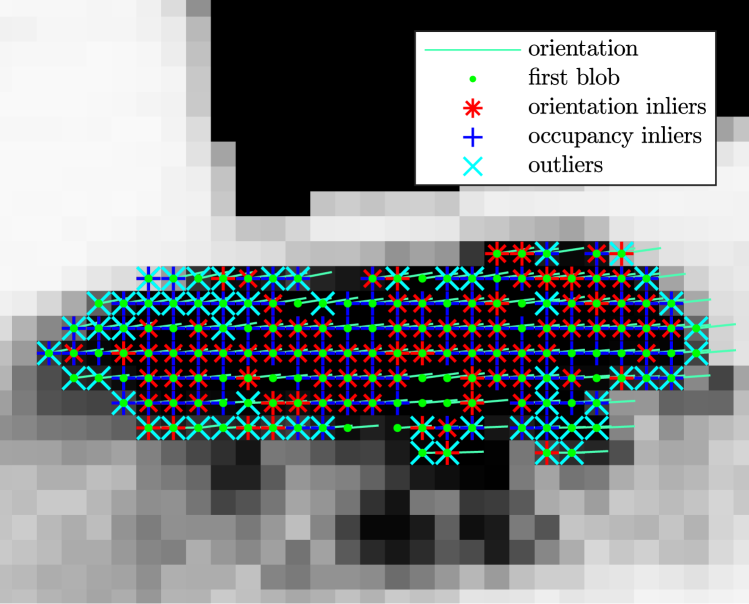
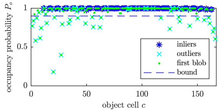
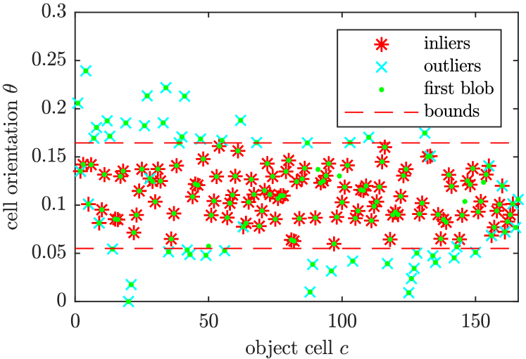
The calculated connected component, based on the starting points from the prediction step, is assumed to include outliers, as the connected component search aims on finding all possible object cells suiting the previous object state. This first connected component is called first blob in Fig. 4 and outlier removal leads to the reduced blob, shown in the same figure. In the removal step only the cells certainly belong together should be taken into account for the shape estimation. The considered properties are

• occupancy value

• orientation value

• velocity value

of every cell in the first blob which results in a mean value and a standard deviation for each property. All cells that lie out of a two-sigma band, i.e. differ more than two standard deviations from the mean, are removed as outliers from the blob. Fig. 5 illustrates the outlier removal in one silhouette. From the previous time step it is known, that the blob consists of $n$ cells. Therefore it is assumed, that the new blob contains $n$ inliers. From the new blob, $n$ cells with highest $P_{\mathrm{O}}$ and lowest deviation from mean orientation $\theta$ are used to calculate the standard deviation, which in turn is used to separate outliers from the first blob. The resulting blob might than contain more than $n$ cells. Please note, that the outlier bounds are limited to a minimum band, i.e. expected variance in the velocity profile and $0.9\cdot\underset{c\in\mathcal{C}_{0}}{\mathrm{max}}\left(P_{\mathrm{O}}(c)\right)$.

V-H Removal of completed object

A fully examined and saved object has to be removed from the searching list. As one object may cover multiple initialization points in each time step of the EMAGS, every affiliated point needs to be removed, spatial as temporal. Algorithm 5 explains how completed objects are removed from the list of initialization points.

Algorithm 5 Object Removal

0:  Object, preprocessed EMAGS

0:  EMAGS without input object

  Extract object dimension

  Transform object in every relevant time step

  Determine underlying cells

  Remove cells from possible initialization points

This step ensures that the algorithm terminates, as it removes at least the initialization point that was considered as possible object. Additionally, as an object is generated by a single initialization point, but may overlap multiple initialization points over different time steps, this step commonly removes more than one point from the stack. Thereby, the calculation time, dependent on the amount of initialized objects, is reduced heavily.

V-I Post Processing

The extracted object trajectory is evaluated for plausible size, shape aspect ratio and smooth movement. Also, trajectories traversing buildings permanently are ignored, while short inference with buildings is tolerated due to localization and map uncertainties. Objects within buildings are usually caused by mirrored laser measurements at glass fronts of buildings. Buildings are represented as polygons obtained from Open Street Maps. It happens that the algorithm traces standing objects. Therefore, static trajectories are ignored. In addition, orientation estimation of objects temporarily standing is error prone and thus corrected using linear interpolation where the trajectory doesn’t move.

VI Results

Figure 6: Example scene of extracted objects with zoomed excerpts a)-d). The occupancy values are illustrated in the background, where moving cells are colored according to their direction. The extracted object labels are shown with orange rectangles. Buildings are plotted with light blue lines, taken from the open street map.

Figure 7: Example scene of extracted objects while the ego vehicle (black rectangle with inner triangle) is moving.

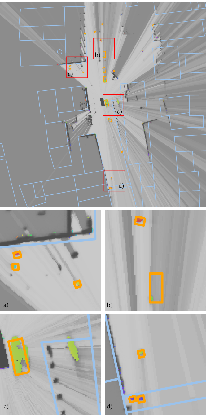
The algorithm was applied on laser recordings from a down town shared space scenarios including multiple pedestrians, bikes, cars, trucks and buses. The experimental vehicle is equipped with multiple laser scanners, four 16-layer Velodyne scanners and one 4-layer Ibeo Lux. The scene was recorded for about $2.5\text{\,}\mathrm{h}$. Although recordings were made with a moving and stationary platform, due to the high traffic, most of the sequence was recorded from a parking position either in the street center or on the sidewalk.

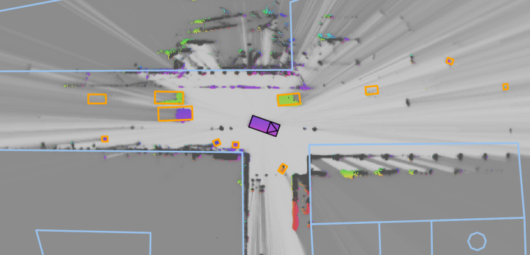
As the presented method generates labels thought as ground truth data, it has to compete with manual labeling and thereby is best validated visually. Fig. 6 shows some examples where the generated object rectangles are plotted in orange, open street map buildings in blue, moving cells in colors according to their direction and the occupancy values in shades of gray. The zoomed excerpts are: a) Three objects (pedestrians) are extracted correctly. b) Two objects (pedestrian and vehicle) are extracted, where the current grid map state would not lead to the correct vehicle size. c) State estimation of the left vehicle fits to the measured cells. The mirrored blob in the right building is omitted, because its trajectory lies inside the building. d) Three pedestrians are correctly extracted, although they are far away from the ego vehicle and close together, which would typically result in one large detection or no detection at all. An example where the ego vehicle is moving is illustrated in Fig. 7. The example shows, that many static regions in the grid map have a false velocity estimation, illustrated by colored grid map pixels. The EMAGS offline assessment, however, resolves that the occupancy is actually not moving although the particle filter indicates dynamic states.

The main limitation of the algorithm is that if track of an object is lost due to temporary full occlusion, reinitialized object tracing easily fails to estimate the correct object size.

VII Conclusion

A new method to generate object labels on a DOGMa is introduced in this work. After the preprocessing of a DOGMa sequence, called EMAGS, the algorithm uses a forward search to find objects and calculate their dimensions and poses. Additionally a backward phase is used to predict the object back to the beginning of the sequence, whereby the best possible object estimation is achieved. The extracted object dimensions and poses serve as automatically generated ground truth labels in the DOGMa. The advantage of this method is that the labels are generated automatically and not manually, thereby it is possible to label almost every amount of sequences, only limited through computation time and not through persons labeling the single images.

References

- [1] Y. Bar-Shalom and T. Fortmann, Tracking and Data Association, ser. Mathematics in Science and Engineering Series. Academic Press, 1988.
- [2] R. P. S. Mahler, Statistical Multisource-Multitarget Information Fusion. Norwood, MA, USA: Artech House, Inc., 2007.
- [3] S. Reuter, A. Scheel, and K. Dietmayer, “The Multiple Model Labeled Multi-Bernoulli Filter,” in Information Fusion (Fusion), 2015 18th International Conference on, July 2015, pp. 1574–1580.
- [4] A. Elfes, “Using Occupancy Grids for Mobile Robot Perception and navigation,” Computer, vol. 22, no. 6, pp. 46–57, June 1989.
- [5] R. Danescu, F. Oniga, and S. Nedevschi, “Modeling and Tracking the Driving Environment With a Particle-Based Occupancy Grid,” IEEE Transactions on Intelligent Transportation Systems, vol. 12, no. 4, pp. 1331–1342, Dec 2011.
- [6] D. Nuss, “A Random Finite Set Approach for Dynamic Occupancy Grid Maps,” Ph.D. dissertation, Universit t Ulm, Institut f r Mess-, Regel- und Mikrotechnik, 2017.
- [7] N. Rexin, D. Nuss, S. Reuter, and K. Dietmayer, “Modeling Occluded Areas in Dynamic Grid Maps,” in 2017 20th International Conference on Information Fusion (Fusion), July 2017, pp. 1–6.
- [8] S. Ulbrich and M. Maurer, “Probabilistic Online POMDP Decision Making for Lane Changes in Fully Automated Driving,” in 16th International IEEE Conference on Intelligent Transportation Systems (ITSC 2013), Oct 2013, pp. 2063–2067.
- [9] M. Ester, H.-P. Kriegel, J. Sander, X. Xu, et al., “A Density-Based Algorithm for Discovering Clusters in Large Spatial Databases with Noise.” in Kdd, vol. 96, no. 34, 1996, pp. 226–231.
- [10] F. Piewak, T. Rehfeld, M. Weber, and J. M. Zöllner, “Fully Convolutional Neural Networks for Dynamic Object Detection in Grid Maps,” CoRR, vol. abs/1709.03139, 2017. [Online]. Available: http://arxiv.org/abs/1709.03139
- [11] S. Hoermann, M. Bach, and K. Dietmayer, “Learning Long-Term Situation Prediction for Automated Driving,” in 2017 16th IEEE International Conference on Machine Learning and Applications (ICMLA), Dec 2017, pp. 1000–1005.
- [12] M. E. Bouzouraa and U. Hofmann, “Fusion of Occupancy Grid Mapping and Model Based Object Tracking for Driver Assistance Systems using Laser and Radar Sensors,” in 2010 IEEE Intelligent Vehicles Symposium, June 2010, pp. 294–300.
- [13] R. Jungnickel and F. Korf, “Object Tracking and Dynamic Estimation on Evidential Grids,” in 17th International IEEE Conference on Intelligent Transportation Systems (ITSC), Oct 2014, pp. 2310–2316.
- [14] M. Sch tz, N. Appenrodt, J. Dickmann, and K. Dietmayer, “Occupancy Grid Map-Based Extended Object Tracking,” in 2014 IEEE Intelligent Vehicles Symposium Proceedings, June 2014, pp. 1205–1210.
- [15] K. Granström and M. Baum, “Extended Object Tracking: Introduction, Overview and Applications,” CoRR, vol. abs/1604.00970, 2016. [Online]. Available: http://arxiv.org/abs/1604.00970
- [16] S. Steyer, G. Tanzmeister, and D. Wollherr, “Object Tracking Based on Evidential Dynamic Occupancy Grids in Urban Environments,” in 2017 IEEE Intelligent Vehicles Symposium (IV), June 2017, pp. 1064–1070.
- [17] T. Yuan, K. Krishnan, B. Duraisamy, M. Maile, and T. Schwarz, “Extended Object Tracking using IMM Approach for a Real-World Vehicle Sensor Fusion System,” in 2017 IEEE International Conference on Multisensor Fusion and Integration for Intelligent Systems (MFI), Nov 2017, pp. 638–643.
- [18] S. Hoermann, P. Henzler, M. Bach, and K. Dietmayer, “Object Detection on Dynamic Occupancy Grid Maps Using Deep Learning and Automatic Label Generation,” ArXiv e-prints, Jan. 2018. [Online]. Available: https://arxiv.org/abs/1802.02202
- [19] A. Dempster, “A generalization of bayesian inference (with diseussion),” Journal of the Royal Statistical Soeiety Series B, vol. 30, no. 2, 1968.