Multi-dimensional Optimal Trade Execution under Stochastic Resilience††thanks: Financial support through the TRCRC 190 Rationality and competition; the economic performance of individuals and firms and d-fine GmbH is gratefully acknowledged. We thank Paulwin Graewe for valuable comments and suggestions. This paper was finished while Horst was visiting the Risk Management Institute at the National University of Singapore. Grateful acknowledgement is made for hospitality.
Abstract
We provide a general framework for analyzing linear-quadratic multi-dimensional portfolio liquidation problems with instantaneous and persistent price impact and stochastic resilience. We show that the value function can be described by a multi-dimensional non-monotone backward stochastic Riccati differential equations (BSRDE) with a singular terminal condition in one component. We prove the existence of a solution to the BSRDE system and characterise both the value function and the optimal strategy in terms of that solution. We prove that the solution to the liquidation problem can be approximated by the solutions to a sequence of unconstrained problems with increasing penalisation of open positions at the terminal time. Our proof is based on a much fine a priori estimate for the approximating BSRDE systems, from which we infer the convergence of the optimal trading strategies for the unconstrained models to an admissible liquidation strategy for the original problem.
Keywords: stochastic control, multi-dimensional backward stochastic Riccati differential equation, multi-dimensional portfolio liquidation, singular terminal value
AMS subject classification: 93E20, 60H15, 91G80
1 Introduction and overview
Let and let be filtered probability space that carries a one dimensional standard Brownian motion . We assume throughout that is the filtration generated by completed by all the null sets and that . For a Euclidean space we denote by and the Banach spaces of all -valued, -adapted, square-integrable stochastic process on , endowed with the norms , respectively .
For any we denote by and the Euclidean space of all symmetric, respectively nonnegative definite matrices. For any two matrices from we write and if is positive definite, respectively nonnegative definite. In what follows all equations and inequalities are to be understood in the -a.s. sense.
For a given we consider the -dimensional linear-quadratic stochastic control problem
| (1.1) |
subject to the state dynamics
| (1.2) |
Here, is positive definite, is a positive definite diagonal matrix, and and are progressively measurable essentially bounded -valued process:
| (1.3) |
Control problems of the above form arise in models of multi-dimensional optimal portfolio liquidation under market impact. In such models, denotes the portfolio the investor needs to liquidate, and denotes the rate at which the different stocks are traded at time . The terminal constraint is the liquidation constraint. The process describes the persistent price impacts caused by past trades. The process describes how fast the order books recover from past trades. The matrix describes an additional instantaneous impact factor. The first two terms of running cost function in (1.1) capture the expected liquidity cost resulting from the instantaneous and the persistent impact, respectively. The third term can be interpreted as a measure of the market risk associated with an open position. It penalises slow liquidation.
The majority of the portfolio liquidation literature allows for only one of the two possible price impacts. The first approach, initiated by Bertsimas and Lo [5] and Almgren and Chriss [2] and later generalized by many authors including [3, 10, 16] describes the price impact as a purely temporary effect that depends only on the present trading rate. A second approach, initiated by Obizhaeva and Wang [17] and later generalized in, e.g. [7, 8] assumes that price impact is persistent with the impact of past trades on current prices decaying over time. Graewe and Horst [9] studied optimal execution problems with instantaneous and persistent price impact and stochastic resilience. In their model the value function can be represented by the solution to a coupled non-monotone three-dimensional stochastic Riccati equation.
In this paper we extend the model in [9] to multi-dimensional portfolios. Our approach uses a penalisation method; we show that the solution to the liquidation problem can be obtained by a sequence of solutions to unconstrained problems where the terminal state constraint is replaced by an increased penalisation of open positions at the terminal time. The penalisation technique has previously been applied to one-dimensional liquidation problems by many authors. When the value function can be characterised by a one-dimensional equation, the monotonicity of value function in the terminal condition can easily be established using standard comparison principles for PDEs or BSDEs. These comparison principles typically do not carry over to higher dimensions, which renders the analysis of multi-dimensional problems, especially the verification result much more complex. We extend the penalisation method to multi-asset liquidation problems with stochastic resilience. As a byproduct we obtain a convergence result for the single-asset model analysed in [9]. The convergence result provides an important consistency result for both the constrained and the unconstrained liquidation problem. Considering sequences of unconstrained problems with increasing penalization of open positions is reasonable only if some form of convergence for the optimal trading strategies can be established. Likewise, the constrained problem should approximate unconstrained problems in some sense.
Several multi-dimensional liquidation models with deterministic cost functions and deterministic resilience have previously been considered in the literature. The special case and in (1.1) and (1.2) corresponds to the multiple asset model of Almgren and Chriss [2]. This model was generalised by Kratz and Schöneborn [15] to discrete-time multi-asset liquidation problems when an investor trades simultaneously in a traditional venue and a dark pool. In the follow-up work [14], the same authors studied a continuous-time multi-asset liquidation problem with dark pools. The benchmark case of deterministic coefficients and zero permanent impact () in (1.2) corresponds to the model in [14] without a dark pool. A model of optimal basket liquidation for a CARA investor with general deterministic cost function was analyzed by Schied et al [19]. In their model there is no loss in generality in restricting the class of admissible liquidation strategies to deterministic ones. Later, Schöneborn [21] considered an infinite-horizon multi-asset portfolio liquidation problem for a general von Neumann-Morgenstern investor with general deterministic temporary and linear permanent impact functions. He characterized the value function as the solution to the two-dimensional PDEs and showed that the optimal portfolio process depends only on the co-variance and cross-asset market impact of the assets in his setting. Alfonsi et al. [1] considered a discrete-time model of optimal basket liquidation with linear transient price impact and general deterministic resilience. Existence of an optimal liquidation strategy in their model is guaranteed if the decay kernel corresponds to a matrix-valued positive definite function but additional assumptions on the decay kernel are required for the optimal liquidation strategies to be well-behaved. In their recent paper, Schneider and Lillo [20] established necessary conditions on the size and impact of cross-impact for the absence of dynamic arbitrage in a continuous time version of [1] that can be directly verified on data.
We provide a general framework for analyzing multi-dimensional portfolio liquidation problems with linear-quadratic cost functions and stochastic resilience. If the cost and the resilience coefficients are described by general adapted stochastic processes, then the value functions can be described by a matrix-valued linear-quadratic backward stochastic Riccati differential equation (BSRDE) with a singular terminal component. In order to prove the existence of optimal liquidation strategies we first analyse the unconstrained problems with finite end costs. We show that the value functions for unconstrained problems are given by the solutions to BSRDE systems with finite terminal value after a linear transformation. For the benchmark case of uncorrelated assets this systems can be decomposed into a series of subsystems for which a priori estimates similar to those in [9] can be established. Using a novel comparison result for matrix-valued BSRDEs given in the appendix, we prove that the solutions to the BSRDE systems can be uniformly bounded from above and below on compact time intervals by two benchmark models with uncorrelated assets. This allows us to prove that the pointwise (in time) limit of the solutions to these systems exists when the degree of penalisation tends to infinity. This limit yields a candidate value function for the liquidation problem.
The verification argument is much more involved. It requires a much finer then usual a priori estimate for the approximating BSRDE systems, from which to infer the convergence of the optimal trading strategies for the unconstrained models to an admissible liquidation strategy for the original problem. The convergence of the optimal strategies allows us to carry out the verification argument and to prove that the limiting BSRDE does indeed characterise the value function of the original liquidation problem. We emphasise that in our multi-dimensional setting the convergence of the optimal trading strategies is required for the verification argument. This is typically not the case in one-dimensional models where much coarser a priori estimates are sufficient to carry out the verification argument.
When all the cost coefficients in our model are deterministic constants, then the value function associated with the optimization problem above can be described by a linear-quadratic ODE system with singular terminal component. The deterministic benchmark case can be analyzed numerically. Our simulations suggest that the correlation between the assets’ fundamental value is a key determinant of optimal liquidation strategies. Consistent with the [9] we also find that when the instantaneous impact factor is low, then the optimal liquidation strategies are strongly convex with the degree of convexity depending on the correlation and the relative liquidity across assets. Surprisingly, a qualitatively similar result is obtained for high persistent impact factors. The intuitive reason is that early trading benefits from resilience.
The remainder of this paper is structured as follows. The model and main results are summarised in Section 2. All proofs are carried out in Section 3. Numerical simulations are provided in Section 4. Section 5 concludes. An appendix contains a multi-dimensional comparison principle for BSRDEs and technical estimates that are omitted in earlier sections.
Notational conventions. We adopt the convention that is a constant, which may vary from line to line. Moreover, we will use the following spaces of progressively measurable processes:
We say that a sequence of stochastic processes converges compactly to on if it converges uniformly to on every compact subinterval. Whenever the notation appears we mean that the statement holds for all the when is replaced by , e.g. . For we mean by - that for every there exists such that for all , -a.e.
For any vector or matrix we put . For the largest (smallest) eigenvalue is denoted () and denotes the induced matrix norm. Then, . For any , the square root exists and and have same eigenvalues. Hence and Moreover, where denotes the identity matrix.
2 Main Results
For any initial state we define by
| (2.1) |
the value function of the stochastic control problem (1.1) subject to the state dynamics
| (2.2) |
Here, the essential infimum is taken over the class of all admissible liquidation strategies, that is over all trading strategies that satisfy the liquidation constraint
We characterise the value function by a unique solution to a matrix-valued backward BSRDE with singular terminal condition. Our approach is based on an approximation argument. To this end, we consider, for any , the value function
| (2.3) |
of a corresponding unconstrained optimisation problem where the liquidation constraint is replaced by a finite penalty term. We solve the unconstrained problem first and then show that the solutions to (2.3) converge to the value function (2.1) as
A pair of random fields is called a classical solution to (2.3) if it satisfies the following conditions:
-
•
for each , is continuously differentiable in and ,
-
•
for each , ,
-
•
for each , ,
-
•
for all and it holds that
(2.4)
The linear-quadratic structure of the control problem suggest the ansatz
| (2.5) |
for the solution to the HJB equation, where are progressively measurable -valued processes. The following lemma shows that this ansatz reduces our HJB equation (2.4) to the matrix-valued stochastic Riccati equation,
| (2.6) | ||||
where is the identity matrix. The proof is standard and hence omitted.
Lemma 2.1.
Bismut [6] and Peng [18] proved the existence and uniqueness of solutions to general BSRDEs, but require the coefficient of degree zero to be nonnegative definite. This requirement is not satisfied in our case. We can overcome this problem by the linear transformation
and by considering the resulting BSRDE:
| (2.8) | ||||
The matrix is nonnegative definite if In this case, all the coefficients in (2.8) satisfy the requirements in [6] and [18] (see also [12, Proposition 2.1]). Hence, we have the following existence result.
Theorem 2.2.
For every the BSRDE (2.8) has a unique solution
The preceding theorem implies the existence and the uniqueness of a solution
to the BSRDE (2.6). The following theorem shows that the solution to the unconstrained optimisation problem can be given in terms of . The proof is given in Section 3 below.
Theorem 2.3.
Intuitively, the solution to (2.1) should be the limit of the solutions to (2.3) as . The following two theorems show that this limit is well-defined and characterises the value function of our liquidation problem. The proofs are given in Section 3 below.
Theorem 2.4.
For any the limit
exists and converges compactly to on Moreover, there exists such that solves the equation
| (2.10) |
on Furthermore,
By Theorem 2.4 we also obtain the existence of the limit of the optimal strategies as
This allows us to state the main result of this paper.
3 Proofs
In this section, we give the proofs of the Theorems 2.3-2.5. In a first step, we bound (with respect to the partial order on the cone of positive semi-definite matrices) the processes by a matrix-valued processes whose limiting behaviour at the terminal time can be inferred from a one-dimensional benchmark model (Lemma 3.1). This will enable us to prove the existence of the limit (Theorem 2.4). In a second step, we establish upper and lower bounds for
near the terminal time (Proposition 3.4), from which we will infer the convergence of the strategies to an admissible liquidation strategy.
Notation. The following notion will be useful. For a generic matrix , we write
| (3.1) |
and set , and .
3.1 A priori estimates
If then and the system (2.8) simplifies to the three-dimensional BSRDE:
| (3.2) |
Analogous to the a priori estimates in [9], we have the following bounds on :
where Thus,
| (3.3) | ||||
3.1.1 A first (rough) estimate
If were diagonal matrices, the BSRDE system (2.8) would separate into subsystems, which are similar to the three-dimensional system (3.2). Our idea is thus to first bound from above and below by diagonal matrices and , respectively, and then to prove that the solutions to the resulting BSRDEs provide upper and lower bounds for the processes .
More precisely, we consider the following BSRDEs:
| (3.4) | ||||
and
| (3.5) | ||||
Their solutions are denoted by and respectively. The matrices are of the form
where each triple solves the BSRDE (3.2) if is replaced by and respectively. Moreover, from our comparison theorem given in the appendix [Theorem A.1], we conclude that the processes , and are nondecreasing in and
| (3.6) |
Combing this inequality with the a priori estimates (3.3), we obtain the following result.
Lemma 3.1.
For every the following a priori estimates hold for all :
| (3.7) | ||||
and where
3.1.2 A second (finer) estimate
We are now going to bound the processes
Multiplying on the left and on the right in (2.8), we see that satisfies
| (3.8) | ||||
Our goal is to bound the processes by the solutions to deterministic RDEs. To this end, we first prove that the process
can be bounded from below and above by and respectively.
Lemma 3.2.
Proof.
Using the matrix decomposition introduced prior to Section 3.1, we need to prove that
Since is nonnegative definite,
In view of (3.1) it follows that,
| (3.11) | ||||
For ,
Set
It is easy to check that
Since is increasing in and we have for Moreover, by Lemma 3.1,
Therefore,
| (3.12) |
This yields the right inequality in (3.10). For the left inequality, notice that similarly to (3.11),
Hence, the left inequality also follows from (3.12). ∎
From [13, Section 2.2.2], we have the following lemma.
Lemma 3.3.
Let where
and let be as in equation (3.9). Then the initial value problems
| (3.13) |
and
| (3.14) |
with
| (3.15) |
possess unique solutions respectively on . They are given by
where
| (3.16) | ||||
with
The matrices in Lemma 3.3 turn out to be the desired bounds for near the terminal time.
Proof.
The preceding proposition established upper and lower bounds for the processes in terms of the functions and on . For analytical convenience we extend these functions and the bounds to the whole interval by putting
| (3.18) | ||||
for and Then,
3.2 Solving the unconstrained problems
In this section, we are going to solve the unconstrained optimisation problem. For any initial state , the dynamics of the state process under the candidate strategy is given by:
| (3.19) |
In particular, and hence
| (3.20) |
where Thus,
| (3.21) | ||||
In order to solve this linear ordinary differential equation, we introduce the fundamental matrix It is given by the unique solution of the ODE system
| (3.22) |
The inverse exists and satisfies
The following lemma establishes norm bounds on the fundamental solution and its inverse.
Lemma 3.5.
Proof.
Let For we obtain by Proposition 3.4 and (3.18) that
Since is discontinuous at if we divide the interval into two subintervals . On each subinterval the assumptions of Gronwall’s inequality are satisfied. Hence,
| (3.24) |
Hence, for all ,
Since is positive definite, and because is the th unit vector this yields
Hence,
This proves the desired bound for the fundamental solution. Since we may consider the differential equation
in order to establish the desired bound for the inverse. This system is similar to (3.22). The desired bounds thus follow from similar arguments as before. ∎
The following bounds on the state process are key to our subsequent analysis.
Proposition 3.6.
Let for as in (2.9). Then there exists a constant that is independent of such that for all
| (3.25) | ||||
Proof.
Let Differentiating this equation and using (3.21) yields,
Since the interated integral version of Gronwall’s inequality yields
| (3.26) | ||||
The processes and are bounded. Moreover, we prove below that there exists a constant , which is independent of such that for
| (3.27) |
Then the desired bounds follow from Lemma 3.5 and Lemma A.2 as
In order to establish the bound (3.27) we multiply on the left and on the right in (2.8) and use the decomposition of the matrix introduced prior to Section 3.1. Thus,
where . Recalling the definition of in (3.22),
The uniform boundedness of together with and yields,
Proposition 3.7.
Proof.
We are now ready to carry out the verification argument for the unconstrained problem (2.3).
Proof of Theorem 2.3.
Let us fix an initial state and admissible control . For we define the stopping time
Since solves the HJB equation, standard arguments show that for any ,
| (3.29) |
where the inequality is an equality if . Since and , it follows from Hölder’s inequality that
and
Thus, the dominated convergence theorem applies when letting in (3.29). This yields
| (3.30) | ||||
with equality if ∎
3.3 Solving the optimal liquidation problem
3.3.1 The candidate value function
In this section, we prove that the limit
exists for . In particular, the candidate value function for (2.1),
is well-defined.
Proof of Theorem 2.4.
For given the sequence is nondecreasing. Moreover, the a priori estimates (3.7) imply that
for some constant uniformly on In particular, the sequence converges pointwise and in to some limiting process on . Using the continuity of ,
This shows that
We are now going to show that is one part of the solution to the matrix differential equation (2.10) on To this end, let and let be the solutions of (2.8) with terminal values and respectively. Applying the Itô formula to on we obtain,
| (3.31) | ||||
where
and
Due to the symmetry of and monotonicity of the sequence , the square root exists. Since is positive definite,
Since the sequence is uniformly bounded on and
for some constant that is independent of Using
| (3.32) |
Moreover, yields,
Hence,
| (3.33) |
Using the Burkholder-Davis-Gundy inequality in (3.31) yields a constant such that
| (3.34) | ||||
By Young’s inequality,
Altogether, we arrive at
The right-hand side converges to zero as This shows that
Furthermore, (3.33) implies that is a Cauchy sequence in and converges to some , for every Taking the limit in (2.8) implies satisfies the matrix differential equation (2.10) on Compact convergence follows by Dini’s theorem, due to the monotonicity. ∎
3.3.2 Verification
Before proving that the strategy defined in Theorem 2.5 is admissible, we first analyse the controlled processes and show that is a liquidation strategy, i.e. that
Proposition 3.8.
-
(i)
Let Then
-
(ii)
In particular,
(3.35)
Proof.
(i) Let On and solve the differential equations
for and , respectively. Since on the sequences and are uniformly bounded and uniformly converges to , the first assertion follows from the continuous dependence of solutions of systems of ordinary linear differential equations on the right side.
(ii) The convergence of the sequence to zero follows from Proposition 3.6 along with Lemma 3.5 and Lemma A.2. From the bound on in (3.17) and the definition of in (3.16), (3.18), we know that
can be bounded from above and below by and respectively.
Therefore, similar argument to the proof of Proposition 3.6 show that
By Lemma A.2, , which yields
Using the uniform boundedness of , similar arguments show that
∎
From the compact convergence results on we know that
Proposition 3.9.
The feedback control is an admissible liquidation strategy.
Proof.
4 Numerical analysis
In this section we simulate the solution to a deterministic benchmark model with two assets. In order to simplify the exposition, we assume that there is no cross asset price impact and choose
| (4.1) |
If all the cost coefficients are deterministic constants, the stochastic Riccati equation reduces to a multi-dimensional ODE system that can be solved numerically using the MATLAB package bvpsuite [11]. This package is designed for solving ODE systems with regular singular points.
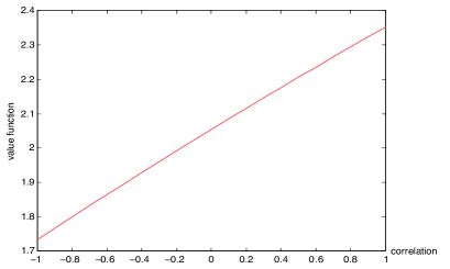
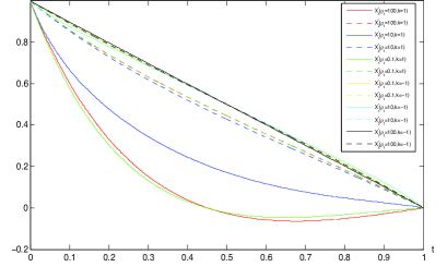
Figure 1 shows that the value function increases in the correlation of the assets’ fundamental price processes. This is natural as a negative correlation reduces risk costs. We also see that for our choice of model parameters the more liquid asset is liquidated at a much faster rate than the less liquid one and that the initial liquidation rate increases in the correlation. Both results are intuitive; fast liquidation reduces risk cost and the cost savings are increasing in the correlation. Moreover, the less liquid asset is liquidated at an almost constant rate while the more liquid asset is liquidated at a convex rate with the degree of convexity decreasing in the correlation.
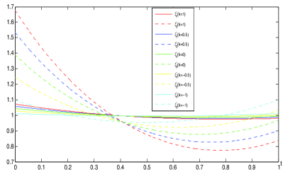
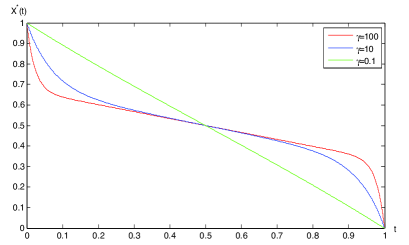
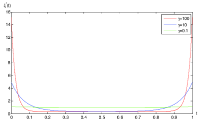
The convexity of the optimal liquidation strategy is consistent with the single asset case analyzed in [9]. There, it is shown that when the instantaneous market impact is small, the optimal liquidation strategy resembles a strategy with block trades: the (single) asset is liquidated at a very high rate initially and close to the terminal time. Similar results for the 2-dimensional case are shown in Figure 2 where the dependence of the value function (left) and the optimal liquidation strategy (right) on the impact factors is depicted.
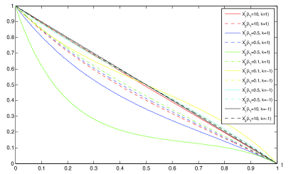
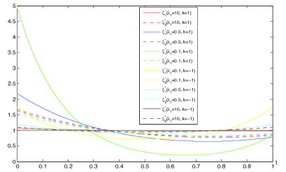
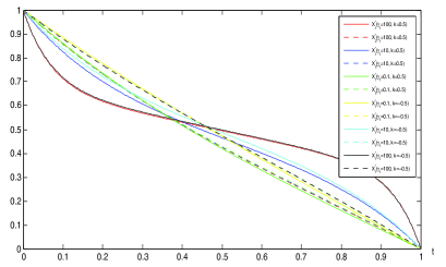
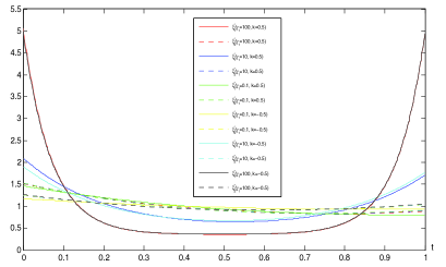
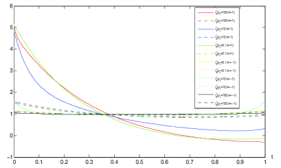
While the initial trading rate decreases if the instantaneous impact factor increases, our simulations suggest that it increases with the persistent impact factors. This effect can already been seen in the single asset case as shown in Figure 3. Simulations for the 2-dimensional case are shown in Figure 4. If the persistent impact factor is large, early trading benefits from resilience. In fact, if there is no resilience and if the persistent impact dominates the cost function to the extend that we may drop the instantaneous impact and risk cost, the resulting Lagrange equation is zero and any liquidation strategy is optimal. If the resilience is positive large initial trades benefit from resilience effects.
The dependence of the optimal solution on the resilience factor is shown in Figure 5. Although we observe again that the optimal strategy is convex, the dependence of the convexity on the strength of resilience is less clear than that on the impact factors. We also see from that figure (red and green curves) that short positions can not be excluded; if the assets are strongly positively correlated, a negative position in one asset may well be beneficial in order to balance the portfolio risk.
5 Conclusion
In this paper we established the existence result of solutions for a multi-dimensional stochastic control problem with singular terminal state constraint. In our model, the value function could be described by a matrix-valued LQ backward stochastic Riccati differential equation with singular terminal component. The verification argument strongly hinged on the a convergence result for the optimal strategies for a series of unconstrained control problems. Several avenues are open for further research. First, as in the one-dimensional case we cannot guarantee non-negativity of the trading rate. Second, the assumption that and are constant was important to establish the a priori estimates. An extension to more general impact factors is certainly desirable. Finally, the set of admissible trading strategies was restricted to absolutely continuous ones. An extension to singular controls would be desirable as well.
Appendix A Appendix
Theorem A.1.
For let , , Assume that
on For , let be the solution of the matrix-valued differential equation,
Then,
Proof.
For given , let be the solution of
on Then,
Thus,
∎
Lemma A.2.
Proof.
In the following proof we introduce simpler bounds for to simplfy the calculations. For where are given by
Hence we need to prove that,
For
For
and
For
and
Therefore, for fixed , there exists a constant independent of such that
∎
References
- [1] A. Alfonsi, F. Klöck, and A. Schied, Multivariate transient price impact and matrix-valued positive definite functions, Math. Oper. Res., 41 (2016), pp. 914–934.
- [2] R. Almgren and N. Chriss, Optimal execution of portfolio transactions, J. Risk, 3 (2001), pp. 5–39.
- [3] S. Ankirchner, M. Jeanblanc, and T. Kruse, BSDEs with singular terminal condition and control problems with constraints, SIAM J. Control Optim., 52 (2014), pp. 893–913.
- [4] D. S. Bernstein, Matrix Mathematics: Theory, Facts, and Formulas with Application to Linear Systems Theory, Princeton University Press, 2005.
- [5] D. Bertsimas and A. W. Lo, Optimal control of execution costs, J. Financ. Markets, 1 (1998), pp. 1–50.
- [6] J.-M. Bismut, Linear quadratic optimal stochastic control with random coefficients, SIAM J. Control Optim., 14 (1976), pp. 419–444.
- [7] A. Fruth, T. Schöneborn, and M. Urusov, Optimal trade execution and price manipulation in order books with time-varying liquidity, Math. Finance, 24 (2014), pp. 651–695.
- [8] , Optimal trade execution in order books with stochastic liquidity. http://homepage.alice.de/murusov/papers/fsu-optimal_execution_stochastic.pdf, 2015.
- [9] P. Graewe and U. Horst, Optimal trade execution with instantaneous price impact and stochastic resilience, SIAM J. Control Optim., 55 (2017), pp. 3707–3725.
- [10] P. Graewe, U. Horst, and J. Qiu, A non-Markovian liquidation problem and backward SPDEs with singular terminal conditions, SIAM J. Control Optim., 53 (2015), pp. 690–711.
- [11] G. Kitzhofer, O. Koch, G. Pulverer, C. Simon, and E. Weinmüller, The new MATLAB code bvpsuite for the solution of singular implicit BVPs, J. Numer. Anal. Indust. Appl. Math., 10 (2010), pp. 113–134.
- [12] M. Kohlmann and S. Tang, Multidimensional backward stochastic riccati equations and applications, SIAM J. Control Optim., 41 (2003), pp. 1696–1721.
- [13] P. Kratz, Optimal liquidation in dark pools in discrete and continuous time, PhD thesis, Humboldt-Universität zu Berlin, 2011.
- [14] P. Kratz and T. Schöneborn, Portfolio liquidation in dark pools in continuous time, Math. Finance, 25 (2015), pp. 496–544.
- [15] P. Kratz and T. Schöneborn, Optimal liquidation in dark pools, Quant. Finance, 14 (2014), pp. 1519–1539.
- [16] T. Kruse and A. Popier, Minimal supersolutions for bsdes with singular terminal condition and application to optimal position targeting, Stochastic Process. Appl., 126 (2016), pp. 2554–2592.
- [17] A. Obizhaeva and J. Wang, Optimal trading strategy and supply/demand dynamics, J. Financ. Markets, 15 (2013), pp. 1–31.
- [18] S. Peng, Stochastic hamilton–jacobi–bellman equations, SIAM J. Control Optim., 30 (1992), pp. 284–304.
- [19] A. Schied, T. Schöneborn, and M. Tehranchi, Optimal basket liquidation for CARA investors is deterministic, Appl. Math. Finance, 17 (2010), pp. 471–489.
- [20] M. Schneider and F. Lillo, Cross-impact and no-dynamic-arbitrage, SSRN, (2016).
- [21] T. Schöneborn, Adaptive basket liquidation, Finance Stoch., 20 (2016), pp. 455–493.