Numerical evidence of electron hydrodynamic whirlpools in graphene samples

Abstract

We present an extension of recent relativistic Lattice Boltzmann methods based on Gaussian quadratures for the study of fluids in $(2+1)$ dimensions. The new method is applied to the analysis of electron flow in graphene samples subject to electrostatic drive; we show that the flow displays hydro-electronic whirlpools in accordance with recent analytical calculations as well as experimental results.

1 Introduction

Relativistic fluid dynamics has so far been generally confined to the study of astrophysical phenomena, and mostly for ideal non-viscous fluids. However, it has been remarked recently that a fluid dynamics approach may be able to capture interesting aspects of the behavior of systems at much smaller scales. A pioneering example is the study of the behavior of the ultra-relativistic quark-gluon plasma formed in the collision of high-energy heavy ions in particle accelerators [1, 2, 3]. More recently, it has been suggested that relativistic fluid dynamics is relevant to understand the behavior of quantum states that can now be studied in several condensed matter experimental setups [4], within the context of so-called AdS-CFT holographic fluids [5, 6, 7, 8].

Recent experimental studies have shown that certain features of the flow of electrons in graphene can be explained through a pseudo-relativistic hydrodynamic approach[9], confirming earlier theoretical predictions [10, 11].

In this paper, we present preliminary results on the development and validation of computationally efficient numerical approaches aimed at capturing details of the electron behavior in these systems, addressing the specific case of graphene.

In brief, electrons in graphene follow an “ultra-relativistic” dispersion relation, so they can be considered as a fluid of massless (quasi-)particles whose energy depends on the momentum as $E=v_{f}p$, with $v_{f}\sim 10^{6}$ m/s the Fermi speed, mimicking the role of the speed of light in true relativistic systems. The observation of hydrodynamic regimes is predicted to be simpler in doped graphene sheets [12], which are characterized by large viscosities.

The Lattice Boltzmann Method (LBM) is a class of computational fluid dynamics solver which has attracted much interest in the past three decades for the solution of the Navier-Stokes equations. The method stems from the kinetic level and consists of a quadrature-based discretization of the Boltzmann equation, allowing the use of a regular grid of points to exactly match the moments of an equilibrium distribution function up to a desired order. Rigorous mathematical analyses based on the Chapman Enskog expansion are typically employed to bridge between the kinetic and the macroscopic level for near equilibrium fluids. Recently, new formulations have been introduced to extend the method to the study of relativistic hydrodynamics. The relativistic Lattice Boltzmann Method (RLBM) [13, 14] offers an appealing solution for the study of dissipative relativistic hydrodynamics, since viscosity is naturally included in its formulation and, furthermore, it does not involve second order derivatives in space, preserving relativistic invariance and causality by construction [15].

The interest towards the numerical study of electrons flow in graphene has motivated the development of two-dimensional RLBM solvers [16, 17, 18, 19]. Most of these numerical methods are based on a second order expansion of an equilibrium distribution function following the Fermi-Dirac statistics, and they have been applied to study e.g. low-viscosity pre-turbulent regimes.

In [20], working in three dimensions, we have shown that third order expansions of the equilibrium distribution function are the minimum requirement to correctly handle dissipative effects in simulations of the relativistic regime.

In this paper, we present a new RLBM in two dimensions, based on a third order expansion of the equilibrium Maxwell-Jüttner distribution. Quantum effects are not described in this model, a choice which simplifies the algorithmic derivation allowing us to retain one of the main LBM features, namely perfect streaming. This could be regarded as the first step in the derivation of a truly accurate model for the fluid dynamics descriptions of electrons in graphene, but we also expect that quantum effects should have a limited impact on the averages involved in hydrodynamical bulk observables. As a result, we expect that the present model should be able to provide new useful insights into the physics of relativistic electron flow in graphene devices. We provide a first validation test of our approach simulating a doped single layer graphene sheet in the so-called ”vicinity-geometry”, which was considered in a series of papers [21, 12, 22] to outline phenomena such as negative nonlocal resistance and current whirlpools. The numerical method is tested in a steady-state regime, for which semi-analytical solutions are available, showing satisfactory agreement with previous works; we wish to emphasize that the present numerical method allows to describe time-dependent, nonlinear flows which escape analytical treatments. Hence, the future plan is to address electron flows of experimental interest.

This paper is organized as follows. In Section 2 we describe our new RLBM model, summarizing the general procedure used in its derivation and providing details of the quadrature and of the external forcing scheme. In Section 3 we carry out simulations of the ”vicinity-geometry” replicating the formation of current whirlpools and providing quantitative comparisons of the electrochemical potential against analytical approximations available in the literature.

2 Model Description

This section briefly describes our RLBM model, which is a ”downsizing” to two spatial dimensions of a similar model handling relativistic flows in 3D; for a more detailed description, the reader is referred to [23, 20].

2.1 Relativistic Boltzmann equation

We consider an ideal non-degenerate relativistic fluid, consisting at the kinetic level of a system of interacting particles of rest mass $m$. The particle distribution function $f((x^{\alpha}),(p^{\alpha}))$, depending on space-time coordinates $\left(x^{\alpha}\right)=\left(ct,\bm{x}\right)$ and momenta $\left(p^{\alpha}\right)=\left(p^{0},\bm{p}\right)=\left(\sqrt{\bm{p}^{2}+m^{2}},\bm{p}\right)$ ($c$ is the speed of light, $\bm{x}$, $\bm{p}\in\mathbb{R}^{2}$), describes the probability of finding a particle with momentum $\bm{p}$ at a given time $t$ and position $\bm{x}$. We adopt Einstein’s summation convention over repeated indexes, and use Greek indexes to denote $(2+1)$ space-time coordinates and Latin indexes for $2$ dimensional spatial coordinates. The particle distribution function obeys the relativistic Boltzmann equation, here taken in the Anderson-Witting [24, 25] relaxation-time approximation:

$$p^{\alpha}\frac{\partial f}{\partial x^{\alpha}}+K^{\alpha}\frac{\partial f}{\partial p^{\alpha}}=\frac{p^{\alpha}U_{\alpha}}{c^{2}~{}\tau}\left(f-f^{eq}\right)\quad,$$ (1)

with $\tau$ the relaxation (proper-)time, $(U^{\alpha})=\gamma\cdot(c,\bm{u})$ the macroscopic $(2+1)$-velocity ($\gamma=1/\sqrt{1-\bm{u}^{2}/c^{2}}$), $K^{\alpha}$ the external forces acting on the system (for simplicity we assume they do not depend on the momentum), and $f^{eq}$ the local equilibrium. In this work $f^{eq}$ will follow a Maxwell-Jüttner distribution:

$$f^{eq}=\frac{1}{A}\exp{\left(-\frac{p^{\alpha}U_{\alpha}}{k_{B}T}\right)}\quad,$$ (2)

where $A$ is a normalization constant and $k_{B}$ the Boltzmann constant.

At the macroscopic level the Anderson-Witting model correctly reproduce the conservation equations, i.e. $\partial_{\alpha}N^{\alpha}=0$ and $\partial_{\beta}T^{\alpha\beta}=0$, with $N^{\alpha}$ the particle $(2+1)$-flow and $T^{\alpha\beta}$ the energy-momentum tensor. At equilibrium $N^{\alpha}$ and $T^{\alpha\beta}$ can be described by the moments of the equilibrium distribution function:

$$N_{E}^{\alpha} =\int f^{eq}p^{\alpha}\frac{\mathop{}\!\mathrm{d}\bm{p}}{p_{0}}=nU^{\alpha}\quad,$$ (3)

$$T_{E}^{\alpha\beta} =\int f^{eq}p^{\alpha}p^{\beta}\frac{\mathop{}\!\mathrm{d}\bm{p}}{p_{0}}=\left(\epsilon+P\right)U^{\alpha}U^{\beta}-P\eta^{\alpha\beta}\quad,$$ (4)

where $n$ is the particle number-density, $\epsilon$ the energy density, $P$ the pressure and $\eta^{\alpha\beta}$ the Minkowski metric tensor. To be noted that the normalization constant in Eq. 2 has to be chosen in such a way to satisfy the relation with the fluid particle density in Eq. 3. In the following we will use $\eta^{\alpha\beta}=diag(1,-1,-1)$, and adopt natural units for which $c=k_{B}=1$ .

2.2 Lattice discretization

In this section we revise the general procedure, used in the derivation of previous non-relativistic [26, 27, 28, 29] and relativistic LBMs [30, 31, 23], for the discretization of the Boltzmann equation on a lattice.

We start from an expansion of the equilibrium distribution function $f^{eq}$ in a basis of polynomials, orthogonal with respect to a weighting function $\omega$ corresponding to $f^{eq}$ in the fluid rest frame (where $\bm{u}=0$). It is simple to verify that in the rest frame Eq. 2 reduces to

$$\omega(p^{0})=\frac{1}{N_{R}}\exp{\left(-p^{0}/T\right)}\quad,$$ (5)

where the normalization factor $N_{R}$ is taken such that $\int\omega(p^{0})\mathop{}\!\mathrm{d}\bm{p}/p^{0}=1$. Starting from the basis $\mathcal{V}=\{1,p^{\alpha},p^{\alpha}p^{\beta},\dots\}$ one derives the set of orthogonal polynomials $\{J^{(i)},i=1,2\dots\}$ by following a Gram-Schmidt procedure, with the inner product defined using the weighting function in Eq. 5. In Appendix A we provide an example of polynomials up to the third order for $m=0$. The polynomials are then used to build the expansion:

$$f^{eq}\left((p^{\mu}),(U^{\mu}),T\right)=\omega(p^{0})\sum_{k=0}^{\infty}a^{(k)}((U^{\mu}),T)J^{(k)}((p^{\mu}))\quad,$$ (6)

where $a^{(k)}$ are the projection coefficients defined as

$$a^{(k)}((U^{\mu}),T)=\int f^{eq}((p^{\mu}),(U^{\mu}),T)J^{(k)}((p^{\mu}))\frac{\mathop{}\!\mathrm{d}\bm{p}}{p^{0}}\quad.$$ (7)

Observe that by construction the coefficients $a^{(k)}$ coincide with the moments of the distribution function; this is a crucial aspect since it follows that $f_{N}^{eq}$, obtained truncating the summation in Eq. 6 such to include only the terms of order up to $N$, correctly preserves the moments of the distribution up to the $N-th$ order.

The next step consists in determining a Gauss-type quadrature on a Cartesian grid, with the aim of i) ensuring exact streaming by requiring that all quadrature points lie on lattice sites ii) preserving the moments of the distribution up to a desired order $N$. The discretized version of the equilibrium distribution can be then written as follows:

$$f_{iN}^{eq}((p^{\mu}),(U^{\mu}),T)=w_{i}\sum_{k=0}^{N}a^{(k)}((U^{\mu}),T)J^{(k)}((p_{i}^{\mu}))\quad.$$ (8)

where $w_{i}$ and $p_{i}^{\mu}$ are the weights and the nodes of the quadrature, respectively. The analytic expression of $f_{iN}^{eq}$ for $N=3$ and $m=0$ is given in Appendix C.

At this stage it is possible to formulate the discrete Boltzmann equation, which in the relativistic case reads as

$$f_{i}(\bm{x}+v^{i}\Delta t,t+\Delta t)-f_{i}(\bm{x},t)=-\Delta t~{}\frac{p_{i}^{\mu}U_{\mu}}{p^{0}\tau}(f_{i}-f_{iN}^{eq})+F^{ext}_{i}\quad.$$ (9)

A detailed description of the algorithmic derivation for the 3-dimensional case is given in [23]. The algebraic complexities in the calculation of the polynomials and the expansion of the equilibrium distribution significantly simplify in 2-D. The full details will be described at length in a future expanded version of this work.

2.3 Quadrature with prescribed nodes

As discussed in the introduction, here we focus our attention on solving Eq. 10 using polynomials up to the third order.

The lattice discretization of the Boltzmann equation can be reduced to a quadrature problem. In practice, one needs to find the weights and the abscissas of a quadrature able to satisfy the orthonormal conditions up to a desired order [32]:

$$\int\omega(p^{0})J_{l}((p^{\mu}))J_{k}((p^{\mu}))\frac{\mathop{}\!\mathrm{d}\bm{p}}{p^{0}}=\sum_{i}w_{i}J_{l}((p^{\mu}_{i}))J_{k}((p^{\mu}_{i}))=\delta_{lk}\quad;$$ (10)

here $p^{\mu}_{i}$ are the discrete quadri-momentum vectors. A convenient parametrization of $p^{\mu}_{i}$ was given in [23] and writes as follows:

$$(p^{\mu}_{i})=p^{0}_{i}(1,v_{0}n_{i})\quad,$$ (11)

where $n_{i}\in\mathbb{Z}^{2}$ are the vectors forming the stencil $G=\{n_{i}~{}|~{}i=1,2,\dots,i_{max}\}$ defined by the (on-lattice) quadrature points, $v_{0}$ is a free parameter that can be freely chosen such that $v_{i}=v_{0}||n_{i}||\leq 1,\forall i$, and $p_{i}^{0}$ is defined as

$$p_{i}^{0}=m\gamma_{i}=m\frac{1}{\sqrt{1-v_{i}^{2}}}\quad.$$ (12)

In order to determine a quadrature we proceed as follows: i) select a value for the rest mass $\bar{m}=m/T_{0}$ (with $T_{0}$ a reference temperature on the lattice), ii) choose a set of velocity vectors $G$, formed by a sufficient number of elements such that the left hand side of Eq. 10 is a full ranked matrix, iii) look for a solution of Eq. 10 formed by non-negative weights $(w_{i}\geq 0,\forall i)$.

We point out that the parametrization in Eq. 11 is general and can be used to determine quadratures for wide ranges of values of $\bar{m}$.

As an example we show in 1(a) a set of vectors that can be used to build a quadrature for $\bar{m}=5$. In the remainder of this paper we are interested in particular in the case of massless particles, all traveling at the same speed $v_{i}=c=1,\forall i$. Since for $m=0$ Eq. 12 is not well defined, we let $p^{0}_{i}$ be free parameters (as already suggested in [31]) to be determined such as to satisfy Eq. 10. We can have several energy shells associated to each vector and therefore we add a second index to Eq. 11:

$$(p^{\mu}_{i,j})=p^{0}_{j}(1,\frac{n_{i}}{||n_{i}||})\quad,$$ (13)

where the index $j$ labels different energy shells.

(a) $\bar{m}=5$, order 3

(b) $\bar{m}=0$, order 3

Figure 1: Examples of stencils for a third-order approximation. Left: $\bar{m}=5$. $G=\{\left(0,0\right),$ $\left(\pm 1,0\right)_{FS},$ $\left(\pm 1,\pm 1\right)_{FS},$ $\left(\pm 2,0\right)_{FS},$ $\left(\pm 2,\pm 1\right)_{FS},$ $\left(\pm 2,\pm 2\right)_{FS},$ $\left(\pm 3,0\right)_{FS},$ $\left(\pm 3,\pm 2\right)_{FS},$ $\left(\pm 3,\pm 3\right)_{FS},$ $\left(\pm 4,0\right)_{FS}$ $\}$ (45 components). Right: $\bar{m}=0$. $G=\{\left(\pm 3,\pm 4\right)_{FS},\left(\pm 5,0\right)_{FS}\}$ with 4 energy shells (48 components).

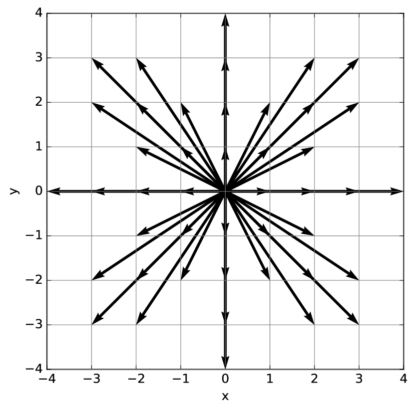
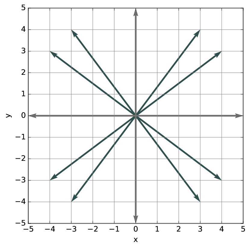
The minimal stencil structure, supporting a third order expansion of the equilibrium distribution function, has radius $R=||n_{i}||=5$ (1(b)); it is formed by the following set of velocity vectors $G=\{\left(\pm 3,\pm 4\right)_{FS},\left(\pm 5,0\right)_{FS}\}$ (FS stands for full symmetric), with four energy shells and the following weights:

$$w_{11} =0.003930503244\dots~{}~{}~{}~{}w_{21}=0.054642060984\dots~{}~{}~{}~{}p^{0}_{1}=0.000016359462\dots$$

$$w_{12} =0.008026424774\dots~{}~{}~{}~{}w_{22}=0.013535762740\dots~{}~{}~{}~{}p^{0}_{2}=3.305423649330\dots$$

$$w_{13} =0.000175706060\dots~{}~{}~{}~{}w_{23}=0.000296310700\dots~{}~{}~{}~{}p^{0}_{3}=7.758786843141\dots$$

$$w_{14} =0.042659667266\dots~{}~{}~{}~{}w_{24}=0.071941262878\dots~{}~{}~{}~{}p^{0}_{4}=0.935838587521\dots$$

$w_{1j}$ and $w_{2j}$, $j=1,\dots,4$ are respectively the weights associated to the stencil components $\left(\pm 3,\pm 4\right)_{FS}$ and $\left(\pm 5,0\right)_{FS}$. This lattice will be used in Section 3 for the numerical part of this work; in Appendix A and Appendix B we list the polynomials and the projections used for the derivation of the method.

2.4 Forcing Scheme

The definition of force in relativity is subject to a certain degree of arbitrariness due to the lack of certain general properties such as, for example, Newton’s third law [33]. In the following we will use the definition of the Minkowski force:

$$K^{\alpha}=m\frac{\mathop{}\!\mathrm{d}U^{\alpha}}{\mathop{}\!\mathrm{d}\tau}\quad,$$ (14)

subject to the condition

$$K^{\alpha}p_{\alpha}=K^{0}p^{0}-\bm{K}\cdot\bm{p}=0\quad,$$ (15)

and

$$\bm{K}=\gamma~{}\bm{F}\quad.$$ (16)

To introduce a forcing term in our numerical scheme we make the following two assumptions: i) the force does not depend on the momentum three vector ( $\frac{\partial K^{\alpha}}{\partial p^{\alpha}}=0$ ) ii) the distribution function in not far from the equilibrium, such that we can approximate the term $K^{\alpha}\frac{\partial f}{\partial p^{\alpha}}$ in Eq. 1 with an expansion that uses the same polynomials used for the equilibrium distribution function:

$$\frac{\partial f}{\partial p^{\alpha}}\approx\frac{\partial f^{eq}}{\partial p^{\alpha}}=\omega(p^{0})\sum_{k=0}^{\infty}b^{(k)}((U^{\mu}),T)J^{(k)}((p^{\mu}))$$ (17)

with the projection coefficients defined as

$$b^{(k)}((U^{\mu}),T)=\int\frac{\partial}{\partial p^{\alpha}}f^{eq}((p^{\mu}),(U^{\mu}),T)J^{(k)}((p^{\mu}))\frac{\mathop{}\!\mathrm{d}\bm{p}}{p^{0}}\quad.$$ (18)

3 Numerical Tests

We now apply the model described in the previous section to the simulation of the (pseudo)-relativistic dynamics of electrons in graphene sheets; as already remarked, in this case the Fermi velocity $v_{f}$ of the simulated system plays the role of the speed of light. We consider an experimental setup consisting of an ultraclean single layer graphene encapsulated between boron nitride crystals in which it has been shown that electrons exhibit a hydrodynamic flow [12]. This setup has been used in a series of works [21, 12, 22] to highlight peculiar properties such as negative nonlocal resistance and current whirlpools.

Figure 2: Geometry used for the validation of the code. Bounce back boundary conditions are imposed at the wall. Sites representing the inlet and the outlet do not evolve in time.

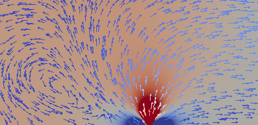
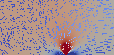
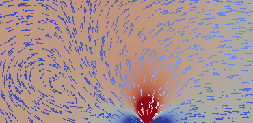
The geometry is sketched in Figure 2. The total force acting on the system is given by the vector sum of the force due to the electric field $F_{E}$ and the force due to the pressure gradient $F_{P}$. While $F_{P}$ is naturally described by our RLBM solver, $F_{E}$ is included in the form of an external force. Therefore, in the simulations the external force $\bm{F}$ (Eq. 16) is given by a self-consistent electric field $\bm{E}=-\rho_{e}\nabla\phi$, with $\rho_{e}=ne$ being the electron charge density. For our initial validation tests on this specific setup, we follow [34] and do not solve explicitly the Poisson equation for the electric potential, but rather use a local capacitance approximation defined as:

$$\phi(\bm{x})=-en(\bm{x})/C_{g}\quad,$$ (19)

where $C_{g}$ is the capacitance per unit area.

Using this setup, we simulate a system similar to the one considered in [21, 12], where analytical results are obtained in the approximation of an infinitely long channel; we use a lattice with an aspect ratio $L/W=4$, that we simulate on a lattice of $2000\times 500$ grid points. The translation between physical units and adimensional lattice units is based on the definition of a length-unit on the lattice such that the width of the channel corresponds to the physical value and on an energy unit that we chose as the Fermi-energy of the simulated system. In Figure 3 we show a snapshot of a simulation, using a constant initial density and a large value for the shear viscosity. As we can see, results are qualitatively comparable with those presented in [21, 12]. In particular one can appreciate the (symmetric) formation of electron back-flows in the proximity of the gates, so called current whirlpools.

Figure 3: Snapshot of a simulation on a $2000\times 500$ lattice, taken after 100000 time steps, with an initial uniform density $n=1.5$, initial $T=1.25$, a fixed velocity at inlet $v^{in}=10^{-5}$, $\tau=1.0$, $C_{g}=10$. The color map describes the electrochemical potential (red colors positive potential, blue colors negative potential). Ticked lines represent the electrons velocity streamlines.

For a more quantitative comparison, we take into consideration the electrochemical potential in the proximity of the injector, for which the following approximate analytic expression was derived in [21]:

$$\Phi(r,\theta)\approx\frac{2I\eta}{\pi\bar{n}^{2}e^{2}}\frac{cos(2\theta)}{r^{2}}\quad;$$ (20)

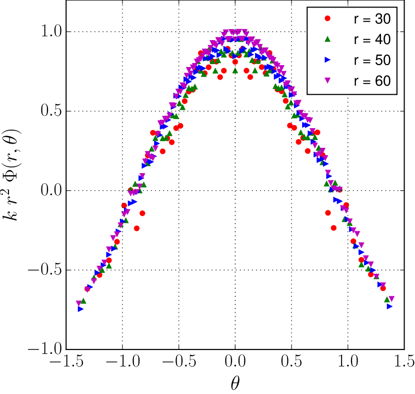
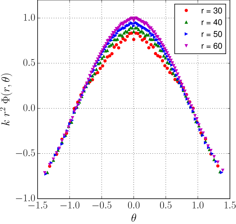
$I$ is the driving current at the inlet, $\eta$ is the shear viscosity, $\bar{n}$ is the equilibrium density, $e$ is the electron charge, $r$ and $\theta$ are used to parametrize in polar coordinates the space in the proximity of the inlet. In Figure 4 we compare the prediction of Eq. 20 with the results of our simulations by plotting the electrochemical potential as a function of the polar angle for several lattice points at several distances $r$ from the center of the injector. In particular we show that for different setups, the quantity $r^{2}~{}\phi(r,\theta)$ does not depend on $r$ as predicted by Equation 20: to a good approximation, all curves collapse on the top of each other, as expected.

Figure 4: Electric potential measured at several fixed distances $r$ from the current injector. Plots present the quantity $r^{2}~{}\Phi(r,\theta)$ normalized to $\Phi(40,0)$, showing that simulated data points collapse onto a single line, as predicted by Eq. 20. Results taken from a simulation on a $2000\times 500$ lattice, with an initial uniform density $n=1.5$, $T=1.25$, $C_{g}=10$ and a fixed velocity at inlet $v^{in}=10^{-5}$ (all quantities in dimensionless units). Left: $\tau=0.8$. Right: $\tau=1.2$.

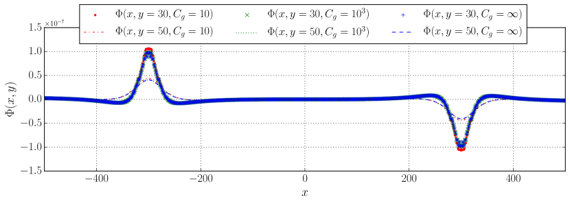
As a further benchmark we evaluate how the steady state solution reported in Figure 3 varies when tuning the magnitude of the driving forces $F_{E}$ and $F_{P}$. To this purpose, we perform simulations with different values of the parameter $C_{g}$ (see Eq. 19) to evaluate the role of the electric potential. Following [35] one would not expect to observe the effect of Coulomb interactions for static flows. In Figure 5 we show that this is indeed the case; in fact varying $C_{g}$ over several different orders of magnitude does not yield any appreciable effect on the solution. Moreover the results are the same even in the case when $F_{E}$ is neglected ($C_{G}=\infty$), proving that the model gives a self-consistent description of hydrodynamic theory on long length scales. On the other hand, the electric potential is expected to play a major role on the dynamics of non-linear, time-dependent flows, which will make the object of forthcoming studies.

(a) $C_{g}=10$

(b) $C_{g}=10^{4}$

(c) $C_{g}=\infty$

(d)

Figure 5: Qualitative (top) and quantitative (bottom) comparison of the electrochemical potential obtained by varying the intensity of the electric field $F_{E}$. Results taken from a simulation on a $2000\times 500$ lattice, with an initial uniform density $n=1.5$, $T=1.25$, $\tau=1.0$ and a fixed velocity at inlet $v^{in}=10^{-5}$ (all quantities in dimensionless units).

4 Conclusions

In this work we have described a new solver for the study of (2+1)-dimensional relativistic hydrodynamics based on the Lattice Boltzmann Method. The model is applied to the specific study case of the analysis of the electrons flow in graphene. We have presented results of simulations of a doped single graphene layer sheet in the so-called ”vicinity-geometry”. From a qualitative point of view we have successfully reproduced the current whirlpools highlighted by recent experimental works [12]. Besides, we have provided a more quantitative validation, with a comparison of the electrochemical potential in the proximity of the current injector against previous analytic predictions [21]. We consider this to be a first step in the derivation of an accurate model for the study of the hydrodynamics behavior of electrons flow in graphene. Future works will deal with more robust comparisons of simulations against experimental data and more detailed simulations of actual experimental setups. This work will allow a proper evaluation of the loss of accuracy due to the neglect of quantum effects, alongside with further parameters that should be taken into account (such as electrons collisions with impurities and phonons) to expand the capabilities of the present model.

Appendix A Third order 2D Relativistic Orthonormal Polynomials

In this appendix we provide the analytic expressions of the relativistic orthogonal polynomials for the ultra-relativistic case up to the third order. The notation $J^{(n)}_{m_{1}\dots m_{n}}$, $m_{i}\in{0,x,y}$ is used to label the polynomial of order $n$ with the subscript $\mu$ referring to the corresponding element of the generating basis $\mathcal{V}=\{1,p^{\alpha},p^{\alpha}p^{\beta}\dots\}$ ($\alpha,\beta\in\{0,x,y\}$):

$$J^{(0)} =1$$

$$J^{(1)}_{0} =p^{0}-1$$

$$J^{(1)}_{x} =p^{x}$$

$$J^{(1)}_{y} =p^{y}$$

$$J^{(2)}_{00} =\frac{1}{2}(p^{0})^{2}-2p^{0}+1$$

$$J^{(2)}_{0x} =\frac{1}{\sqrt{3}}p^{0}p^{x}-\sqrt{3}p^{x}$$

$$J^{(2)}_{0y} =\frac{1}{\sqrt{3}}p^{0}p^{y}-\sqrt{3}p^{y}$$

$$J^{(2)}_{xx} =\frac{1}{\sqrt{3}}(p^{x})^{2}-\frac{1}{2\sqrt{3}}(p^{0})^{2}$$

$$J^{(2)}_{xy} =\frac{1}{\sqrt{3}}p^{x}p^{y}$$

$$J^{(3)}_{000} =\frac{1}{6}(p^{0})^{3}-\frac{3}{2}(p^{0})^{2}+3p^{0}-1$$

$$J^{(3)}_{xxx} =-p^{0}p^{x}+\frac{1}{6}(p^{x})^{3}+\frac{3}{2}p^{x}$$

$$J^{(3)}_{00x} =\frac{1}{\sqrt{15}}(p^{0})^{2}p^{x}-\sqrt{\frac{5}{3}}p^{0}p^{x}-\frac{1}{2\sqrt{15}}(p^{x})^{3}+\frac{\sqrt{15}}{2}p^{x}$$

$$J^{(3)}_{0xx} =-\frac{1}{2\sqrt{15}}(p^{0})^{3}+\frac{1}{2}\sqrt{\frac{5}{3}}(p^{0})^{2}+\frac{1}{\sqrt{15}}p^{0}(p^{x})^{2}-\sqrt{\frac{5}{3}}(p^{x})^{2}$$

$$J^{(3)}_{00y} =\frac{1}{2\sqrt{6}}(p^{0})^{2}p^{y}-2\sqrt{\frac{2}{3}}p^{0}p^{y}+\sqrt{6}p^{y}$$

$$J^{(3)}_{xxy} =\frac{1}{3}\sqrt{\frac{2}{5}}(p^{x})^{2}p^{y}-\frac{1}{6\sqrt{10}}(p^{0})^{2}p^{y}$$

$$J^{(3)}_{0xy} =\frac{1}{\sqrt{15}}p^{0}p^{x}p^{y}-\sqrt{\frac{5}{3}}p^{x}p^{y}$$

Appendix B Third order 2D Orthogonal Projections

In this appendix we provide the analytic expressions of the orthogonal projections $a^{(k)}$, up to the third order, for the ultra-relativistic case. The notation follows the one introduced in Appendix A for the orthogonal polynomials. All the projections are scaled with the particle density $n$, thereby ensuring the correct normalization of the equilibrium distribution function (Eq. 2).

$$a^{(0)} =1$$

$$a^{(1)}_{0} =Tu^{0}-1$$

$$a^{(1)}_{x} =Tu^{x}$$

$$a^{(1)}_{y} =Tu^{y}$$

$$a^{(2)}_{00} =\frac{1}{2}T^{2}\left(3(u^{0})^{2}-1\right)-2Tu^{0}+1$$

$$a^{(2)}_{0x} =\sqrt{3}Tu^{x}(Tu^{0}-1)$$

$$a^{(2)}_{0y} =\sqrt{3}Tu^{y}(Tu^{0}-1)$$

$$a^{(2)}_{xx} =-\frac{1}{2}\sqrt{3}T^{2}\left((u^{0})^{2}-2(u^{x})^{2}-1\right)$$

$$a^{(2)}_{xy} =\sqrt{3}T^{2}u^{x}u^{y}$$

$$a^{(3)}_{000} =\frac{1}{2}(Tu^{0}-1)\left(T^{2}\left(5(u^{0})^{2}-3\right)-4T(u^{0})+2\right)$$

$$a^{(3)}_{xxx} =\frac{1}{2}Tu^{x}\left(T^{2}\left(5(u^{x})^{2}+3\right)-6Tu^{0}+3\right)$$

$$a^{(3)}_{00x} =-\frac{1}{2}\sqrt{15}Tu^{x}\left(T^{2}\left(-2(u^{0})^{2}+(u^{x})^{2}+1\right)+2Tu^{0}-1\right)$$

$$a^{(3)}_{0xx} =-\frac{1}{2}\sqrt{15}T^{2}(Tu^{0}-1)\left((u^{0})^{2}-2(u^{x})^{2}-1\right)$$

$$a^{(3)}_{00y} =\frac{1}{2}\sqrt{\frac{3}{2}}Tu^{y}\left(T^{2}\left(5(u^{0})^{2}-1\right)-8Tu^{0}+4\right)$$

$$a^{(3)}_{xxy} =-\frac{1}{2}\sqrt{\frac{5}{2}}T^{3}u^{y}\left((u^{0})^{2}-4(u^{x})^{2}-1\right)$$

$$a^{(3)}_{0xy} =\sqrt{15}T^{2}u^{x}u^{y}(Tu^{0}-1)$$

Appendix C Third order expansion of the equilibrium distribution function

The third order expansion of the Maxwell-Jüttner distribution in two dimension and for $m=0$, which allows to recover the first, the second and the third order moments of Eq. 2, was derived using the polynomials defined in Appendix A and projections in Appendix B. It reads as follow:

$$f_{i}^{eq} =\frac{w_{i}~{}n}{T}\left(\frac{1}{6}T^{3}u^{x}\left((p_{i}^{x})^{3}-\frac{3(p_{i}^{0})^{2}p_{i}^{x}}{4}\right)\left(-3(u^{0})^{2}+4(u^{x})^{2}+3\right)\right.$$

$$\left.+\frac{1}{24}p_{i}^{y}T^{3}u^{y}\left((p_{i}^{0})^{2}-4(p_{i}^{x})^{2}\right)\left((u^{0})^{2}-4(u^{x})^{2}-1\right)\right.$$

$$\left.+\frac{1}{4}T^{2}\left((p_{i}^{0})^{2}-2(p_{i}^{x})^{2}\right)\left((u^{0})^{2}-2(u^{x})^{2}-1\right)+\frac{1}{8}\left(-2(p_{i}^{0})^{2}+(p_{i}^{0}-5)(p_{i}^{x})^{2}\right.\right.$$

$$\left.\left.+9p_{i}^{0}-3\right)(Tu^{0}-1)\left(T\left(5T(u^{x})^{2}+T-2u^{0}\right)+1\right)+\frac{1}{24}\left(4(p_{i}^{0})^{3}-30(p_{i}^{0})^{2}\right.\right.$$

$$\left.\left.-3(p_{i}^{0}-5)(p_{i}^{x})^{2}+45p_{i}^{0}-15\right)(Tu^{0}-1)\left(T^{2}\left(4(u^{0})^{2}-3\left((u^{x})^{2}+1\right)\right)\right.\right.$$

$$\left.\left.-2Tu^{0}+1\right)+(p_{i}^{0}-5)p_{i}^{x}p_{i}^{y}T^{2}u^{x}u^{y}(Tu^{0}-1)\right.$$

$$\left.+\frac{1}{8}(p_{i}^{0}-6)(p_{i}^{0}-2)p_{i}^{x}Tu^{x}\left(T^{2}\left(5(u^{0})^{2}-1\right)-8Tu^{0}+4\right)\right.$$

$$\left.+(p_{i}^{0}-3)p_{i}^{x}Tu^{x}(Tu^{0}-1)+\frac{1}{8}(p_{i}^{0}-6)(p_{i}^{0}-2)p_{i}^{y}T(u^{y})\left(T^{2}\left(5(u^{0})^{2}-1\right)\right.\right.$$

$$\left.\left.-8Tu^{0}+4\right)+(p_{i}^{0}-3)p_{i}^{y}Tu^{y}(Tu^{0}-1)+\frac{1}{4}((p_{i}^{0}-4)p_{i}^{0}+2)\left(T^{2}\left(3(u^{0})^{2}\right.\right.\right.$$

$$\left.\left.\left.-1\right)-4Tu^{0}+2\right)+(p_{i}^{0}-1)(Tu^{0}-1)+p_{i}^{x}p_{i}^{y}T^{2}u^{x}u^{y}+p_{i}^{x}Tu^{x}+p_{i}^{y}Tu^{y}+1\right)$$

References

- [1] U. Heinz, R. Snellings, Collective flow and viscosity in relativistic heavy-ion collisions, Annual Review of Nuclear and Particle Science 63 (1) (2013) 123–151. doi:10.1146/annurev-nucl-102212-170540.
- [2] W. Florkowski, M. P. Heller, M. Spalinski, New theories of relativistic hydrodynamics in the lhc era, Reports on Progress in Physics.
- [3] P. Romatschke, Far From Equilibrium Fluid DynamicsarXiv:1704.08699.
- [4] E. Fradkin, S. A. Kivelson, M. J. Lawler, J. P. Eisenstein, A. P. Mackenzie, Nematic Fermi Fluids in Condensed Matter Physics, Annual Review of Condensed Matter Physics 1 (1) (2010) 153–178. doi:10.1146/annurev-conmatphys-070909-103925.
- [5] J. Maldacena, The Large-N Limit of Superconformal Field Theories and Supergravity, International Journal of Theoretical Physics 38 (4) (1999) 1113–1133. doi:10.1023/A:1026654312961.
- [6] P. K. Kovtun, D. T. Son, A. O. Starinets, Viscosity in strongly interacting quantum field theories from black hole physics, Phys. Rev. Lett. 94 (2005) 111601. doi:10.1103/PhysRevLett.94.111601.
- [7] S. Bhattacharyya, S. Minwalla, V. E. Hubeny, M. Rangamani, Nonlinear fluid dynamics from gravity, Journal of High Energy Physics 2008 (02) (2008) 045.
- [8] R. Baier, P. Romatschke, D. T. Son, A. O. Starinets, M. A. Stephanov, Relativistic viscous hydrodynamics, conformal invariance, and holography, Journal of High Energy Physics 2008 (04) (2008) 100.
- [9] J. Crossno, J. K. Shi, K. Wang, X. Liu, A. Harzheim, A. Lucas, S. Sachdev, P. Kim, T. Taniguchi, K. Watanabe, T. A. Ohki, K. C. Fong, Observation of the Dirac fluid and the breakdown of the Wiedemann-Franz law in graphene, Sciencedoi:10.1126/science.aad0343.
- [10] M. Müller, L. Fritz, S. Sachdev, Quantum-critical relativistic magnetotransport in graphene, Phys. Rev. B 78 (2008) 115406. doi:10.1103/PhysRevB.78.115406.
- [11] M. Müller, J. Schmalian, L. Fritz, Graphene: A nearly perfect fluid, Phys. Rev. Lett. 103 (2009) 025301. doi:10.1103/PhysRevLett.103.025301.
- [12] D. A. Bandurin, I. Torre, R. K. Kumar, M. Ben Shalom, A. Tomadin, A. Principi, G. H. Auton, E. Khestanova, K. S. Novoselov, I. V. Grigorieva, L. A. Ponomarenko, A. K. Geim, M. Polini, Negative local resistance caused by viscous electron backflow in graphene, Sciencedoi:10.1126/science.aad0201.
- [13] M. Mendoza, B. M. Boghosian, H. J. Herrmann, S. Succi, Fast lattice boltzmann solver for relativistic hydrodynamics, Phys. Rev. Lett. 105 (2010) 014502. doi:10.1103/PhysRevLett.105.014502.
- [14] M. Mendoza, B. M. Boghosian, H. J. Herrmann, S. Succi, Derivation of the lattice boltzmann model for relativistic hydrodynamics, Phys. Rev. D 82 (2010) 105008. doi:10.1103/PhysRevD.82.105008.
- [15] P. Romatschke, U. Romatschke, Relativistic Fluid Dynamics Out of Equilibrium (December). arXiv:1706.00801.
- [16] M. Mendoza, H. J. Herrmann, S. Succi, Preturbulent Regimes in Graphene Flow, Phys. Rev. Lett. 106 (15) (2011) 156601. arXiv:1201.6590, doi:10.1103/PhysRevLett.106.156601.
- [17] D. Oettinger, M. Mendoza, H. J. Herrmann, Gaussian quadrature and lattice discretization of the Fermi-Dirac distribution for graphene, Phys. Rev. E 88 (2013) 013302. doi:10.1103/PhysRevE.88.013302.
- [18] O. Furtmaier, M. Mendoza, I. Karlin, S. Succi, H. J. Herrmann, Rayleigh-Bénard instability in graphene, Phys. Rev. B 91 (2015) 085401. doi:10.1103/PhysRevB.91.085401.
- [19] R. C. V. Coelho, M. Mendoza, M. M. Doria, H. J. Herrmann, Kelvin-Helmholtz instability on graphene (June). arXiv:1706.00801.
- [20] A. Gabbana, M. Mendoza, S. Succi, R. Tripiccione, Kinetic approach to relativistic dissipation, Phys. Rev. E 96 (2017) 023305. doi:10.1103/PhysRevE.96.023305.
- [21] I. Torre, A. Tomadin, A. K. Geim, M. Polini, Nonlocal transport and the hydrodynamic shear viscosity in graphene, Phys. Rev. B 92 (2015) 165433. doi:10.1103/PhysRevB.92.165433.
- [22] F. M. D. Pellegrino, I. Torre, A. K. Geim, M. Polini, Electron hydrodynamics dilemma: Whirlpools or no whirlpools, Phys. Rev. B 94 (2016) 155414. doi:10.1103/PhysRevB.94.155414.
- [23] A. Gabbana, M. Mendoza, S. Succi, R. Tripiccione, Towards a unified lattice kinetic scheme for relativistic hydrodynamics, Phys. Rev. E 95 (2017) 053304. doi:10.1103/PhysRevE.95.053304.
- [24] J. Anderson, H. Witting, A relativistic relaxation-time model for the Boltzmann equation, Physica 74 (3) (1974) 466 – 488. doi:10.1016/0031-8914(74)90355-3.
- [25] J. Anderson, H. Witting, Relativistic quantum transport coefficients, Physica 74 (3) (1974) 489 – 495. doi:10.1016/0031-8914(74)90356-5.
- [26] F. J. Higuera, S. Succi, R. Benzi, Lattice gas dynamics with enhanced collisions, EPL (Europhysics Letters) 9 (4) (1989) 345.
- [27] X. He, L.-S. Luo, Theory of the lattice Boltzmann method: From the Boltzmann equation to the lattice Boltzmann equation, Phys. Rev. E 56 (1997) 6811–6817. doi:10.1103/PhysRevE.56.6811.
- [28] X. Shan, X. He, Discretization of the velocity space in solution of the Boltzmann equationdoi:10.1103/PhysRevLett.80.65.
- [29] N. S. Martys, X. Shan, H. Chen, Evaluation of the external force term in the discrete Boltzmann equation, Phys. Rev. E 58 (1998) 6855–6857. doi:10.1103/PhysRevE.58.6855.
- [30] P. Romatschke, M. Mendoza, S. Succi, Fully relativistic lattice Boltzmann algorithm, Phys. Rev. C 84 (2011) 034903. doi:10.1103/PhysRevC.84.034903.
- [31] M. Mendoza, I. Karlin, S. Succi, H. J. Herrmann, Relativistic lattice Boltzmann model with improved dissipation, Phys. Rev. D 87 (2013) 065027. doi:10.1103/PhysRevD.87.065027.
- [32] P. C. Philippi, L. A. Hegele, L. O. E. dos Santos, R. Surmas, From the continuous to the lattice Boltzmann equation: The discretization problem and thermal models, Phys. Rev. E 73 (2006) 056702. doi:10.1103/PhysRevE.73.056702.
- [33] M. Tuval, A. Yahalom, Newton’s third law in the framework of special relativity, The European Physical Journal Plus 129 (11) (2014) 240. doi:10.1140/epjp/i2014-14240-x.
- [34] A. Tomadin, M. Polini, Theory of the plasma-wave photoresponse of a gated graphene sheet, Phys. Rev. B 88 (2013) 205426. doi:10.1103/PhysRevB.88.205426.
- [35] A. Lucas, J. Crossno, K. C. Fong, P. Kim, S. Sachdev, Transport in inhomogeneous quantum critical fluids and in the Dirac fluid in graphene, Phys. Rev. B 93 (2016) 075426. doi:10.1103/PhysRevB.93.075426.