Higher-Order Nonlinear Complementary Filtering on Lie Groups

David Evan Zlotnik,  James Richard Forbes This research was supported by the National Science Foundation Award Number 1550103. D. E. Zlotnik is with the Department of Aerospace Engineering, University of Michigan, Ann Arbor, MI, 48109 USA e-mail: dzlotnik@umich.edu.J. R. Forbes is with the Department of Mechanical Engineering, McGill University, Montreal, QC, H3A 0C3, Canada e-mail: james.richard.forbes@mcgill.ca.
Abstract

Nonlinear observer design for systems whose state space evolves on Lie groups is considered. The proposed method is similar to previously developed nonlinear observers in that it involves propagating the state estimate using a process model and corrects the propagated state estimate using an innovation term on the tangent space of the Lie group. In the proposed method, the innovation term is constructed by passing the gradient of an invariant cost function, resolved in a basis of the tangent space, through a linear time-invariant system. The introduction of the linear system completes the extension of linear complementary filters to nonlinear Lie group observers by allowing higher-order filtering. In practice, the proposed method allows for greater design freedom and, with the appropriate selection of the linear filter, the ability to filter bias and noise over specific bandwidths. A disturbance observer that accounts for constant and harmonic disturbances in group velocity measurements is also considered. Local asymptotic stability about the desired equilibrium point is demonstrated. A numerical example that demonstrates the desirable properties of the observer is presented in the context of pose estimation.

I Introduction

The kinematics and dynamics of many systems evolve on differential manifolds, rather than strictly in Euclidean space. Lie groups are a well known class of manifold that occur naturally in the study of rigid-body kinematics. Attitude kinematics, for example, evolve on the Lie group SO(3)𝑆𝑂3SO(3), while pose kinematics evolve on the special Euclidean group SE(3)𝑆𝐸3SE(3) [1]. The development of observers for systems whose state evolves on a Lie group is therefore a highly practical exercise. A class of nonlinear Lie group observers has recently been developed [2, 3, 4, 5, 6, 7]. The interest in these observers was, in part, sparked by the development of nonlinear observers for attitude estimation using first the unit quaternion [8, 9, 10, 11] and later the rotation matrix element of SO(3)𝑆𝑂3SO(3) directly [12, 13]. Following [13], several nonlinear attitude observers that exploit the underlying SO(3)𝑆𝑂3SO(3) Lie group structure have been developed [14, 15, 16], as well as several SE(3)𝑆𝐸3SE(3) based nonlinear observers [17, 18]. By working directly with the elements of SO(3)𝑆𝑂3SO(3) and SE(3)𝑆𝐸3SE(3), the attitude and pose are both globally and uniquely represented and thus issues associated with attitude parameterizations, such as non-uniqueness, are avoided [19]. Nonlinear observers are attractive as they can often be shown to have strong stability properties [11, 5, 6] and are, in general, computationally simpler than traditional estimation methods [5].

Lie group observer design methodology considered in the literature can often be described as possessing two distinct terms. The first is a copy of the nonlinear system while the second is an innovation term that serves to drive the estimated state towards the true state. This is analogous to the Luenberger observer for linear systems where the state estimate is propogated using a process model and a correction term alters the state estimate based on the error between the measured and estimated system output. However, as mentioned in [5], there is no canonical choice for the innovation term for Lie group observers, and as such, its selection must be carefully considered. A method to find suitable innovation terms is considered in [2], where symmetry preserving innovation terms are found via the moving frame method [2, 6]. Alternatively, in [3] and [5] the innovation term is chosen based on the gradient descent direction of a selected invariant cost function and the observer is shown to be almost globally asymptotically stable about the point where the estimated state is equal to the true state. The work of [5] was extended in [6] where a nonlinear Lie group observer for systems with homogeneous outputs and biased velocity measurements was proposed.

In this paper, a nonlinear observer whose system state evolves on a Lie group is considered. The approach taken is similar to previous Lie group observers presented in the literature, including [5], [6], as the innovation is related to the gradient of a cost function. However, while the gradient of the cost function appears directly as the innovation term in [5], in this paper the innovation is based on the output of a linear time-invariant (LTI) system whose input is the gradient of a cost function resolved in a basis of the tangent space. Analogous to the classical complementary filter, the proposed method can be understood as a nonlinear complementary filter on a Lie group. Previous observers, including [5] and [6], are analogous to the classical complementary filter with first order sensitivity and complementary sensitivity transfer functions. The introduction of the LTI system in the proposed observer allows for more general and complex higher-order filtering. Consequently, to the authors’ knowledge, the proposed method is the first nonlinear observer that fully extends the concept of linear complementary filtering to Lie group observer design. This is highly practical, as it allows for the targeting of specific frequency bandwidths in the velocity and partial state measurements. For example, applying a fast Fourier transform (FFT) to measurement data, the frequency content of the measurement noise can be identified and then mitigated by carefully constructing the LTI system. Further, it is shown that by restricting the LTI sytem to the set of strictly positive real systems with feedthrough the strong stability properties of the nonlinear observer can be maintained. Passing nonlinear inputs through dynamic systems are considered in the context of rigid-body attitude estimation in [20] and [21], and for rigid-body attitude control in [22]. In [22] the nonlinear input is passed through a first-order dynamic system where the dynamic system is used to retain continuity in the case of discontinuities in the nonlinear input. In [20] and [21], a first-order dynamic system is employed and is derived via the Lagrange-D’Alembert principle and applied in continuous and discrete time. The filters in [20], [21], and [22] are first-order and consequently do not generalize to higher-order systems. Further, they were developed for the specific case of the Lie group SO(3)𝑆𝑂3SO(3), while general Lie groups are considered in this paper.

The inclusion of an LTI system for filtering on the Lie group SO(3)𝑆𝑂3SO(3) has been previously considered in [23]. This paper builds upon the results of [23] by considering a general Lie group as well as considering the effects of harmonic disturbances, both of which constitute significant contributions. Moreover, full state measurements of the rotation matrix element of SO(3)𝑆𝑂3SO(3) is assumed in [23], while the more realistic scenario of partial state measurements are assumed in this paper. Further, the proposed method is a direct extension of the gradient observer proposed in [5] in that the proposed observer reduces to the gradient observer with the selection of a particular static linear system. As in [6] and [7], the case where velocity measurements are corrupted by constant bias is also considered. However, the solutions given in [6] and [7] are extended in this paper to include harmonic disturbances as well as constant bias. This is done by introducing a disturbance observer that incorporates an internal model of the harmonic disturbances. In practice, harmonic disturbances may be introduced due to mechanical vibration of a vehicle’s structure or mechanical imbalance of rotors. For example, mounting an inertial measurement unit on a stiff but not infinitely rigid aerial vehicle frame would introduce harmonic disturbances into the angular velocity measurement [24]. The approach taken is similar to the method given in [24], where an adaptive disturbance observer is proposed in the context of attitude estimation. In this paper a disturbance observer for use with any general Lie group is considered.

The main contribution of this paper is the design of the observer, which allows for greater design freedom compared to similar observers and can, with appropriate selection of the LTI system, result in enhanced rejection of measurement noise. It is shown that, provided the linear system is composed of a strictly positive real part and feedthrough, the proposed observer is locally asymptotically stable about a desired equilibrium point.

The remainder of this paper is as follows. Mathematical preliminaries are discussed in Sec. II including a discussion on Lie groups as well as Riemannian geometry. Observer design is considered in Sec. III, where stability results are presented in Sec. III-C. The disturbance observer is introduced in Sec. IV. The proposed observer is demonstrated in the context of rigid-body pose estimation in Sec. V. Finally, concluding remarks are given in Sec. VI.

II Mathematical Preliminaries and Notation

We adopt notation from [1], [25], [5] and [7]. Following [5], let G𝐺G and 𝔤𝔤\mathfrak{g} respectively denote a finite dimensional connected Lie group and its associated Lie algebra. An inner product on 𝔤𝔤\mathfrak{g} is denoted ,:𝔤×𝔤:𝔤𝔤\langle\cdot,\cdot\rangle:\mathfrak{g}\times\mathfrak{g}\rightarrow\mathbb{R} with associated norm ||||𝔤=,||\cdot||_{\mathfrak{g}}=\sqrt{\langle\cdot,\cdot\rangle}. Further, let IG𝐼𝐺I\in G be the identity element and for X,YG𝑋𝑌𝐺X,Y\in G, and define the right and left translation maps by RX:GG,YYX:subscript𝑅𝑋formulae-sequence𝐺𝐺maps-to𝑌𝑌𝑋R_{X}:G\rightarrow G,Y\mapsto YX and LX:GG,YXY:subscript𝐿𝑋formulae-sequence𝐺𝐺maps-to𝑌𝑋𝑌L_{X}:G\rightarrow G,Y\mapsto XY [1]. The tangent space of G𝐺G at any point XG𝑋𝐺X\in G is denoted TXGsubscript𝑇𝑋𝐺T_{X}G. Given XG𝑋𝐺X\in G and v𝔤𝑣𝔤v\in\mathfrak{g}, vectors in TXGsubscript𝑇𝑋𝐺T_{X}G may be expressed as Xv𝑋𝑣Xv or vX𝑣𝑋vX, where Xv𝑋𝑣Xv and vX𝑣𝑋vX denote a simplified notation for TILXvsubscript𝑇𝐼subscript𝐿𝑋𝑣T_{I}L_{X}v and TIRXvsubscript𝑇𝐼subscript𝑅𝑋𝑣T_{I}R_{X}v, respectively [5, 25]. The adjoint map, denoted AdX:𝔤𝔤:subscriptAd𝑋𝔤𝔤{\mathrm{Ad}}_{X}:\mathfrak{g}\rightarrow\mathfrak{g}, is a linear map where AdX(v)=TXRX1TILXvsubscriptAd𝑋𝑣subscript𝑇𝑋subscript𝑅superscript𝑋1subscript𝑇𝐼subscript𝐿𝑋𝑣{\mathrm{Ad}}_{X}(v)=T_{X}R_{X^{-1}}T_{I}L_{X}v for all XG𝑋𝐺X\in G and v𝔤𝑣𝔤v\in\mathfrak{g} [7].

Let the set B={b1,,bn}𝐵subscript𝑏1subscript𝑏𝑛B=\{b_{1},\ldots,b_{n}\}, where b1,,bn𝔤subscript𝑏1subscript𝑏𝑛𝔤b_{1},\ldots,b_{n}\in\mathfrak{g}, be a basis of 𝔤𝔤\mathfrak{g}. Then, for any a𝔤𝑎𝔤a\in\mathfrak{g}, a𝑎a may be written as a=S(𝐚)𝑎𝑆𝐚a=S(\mbf{a}) where 𝐚=[𝐚𝟏,,𝐚𝐧]𝖳𝐧𝐚superscriptsubscript𝐚1subscript𝐚𝐧𝖳superscript𝐧\mbf{a}=[\ a_{1},\ldots,a_{n}\ ]^{\mathsf{T}}\in\mathbb{R}^{n} and S:n𝔤:𝑆superscript𝑛𝔤S:\mathbb{R}^{n}\rightarrow\mathfrak{g} is such that S(𝐚)=𝐢=𝟏𝐧𝐚𝐢𝐛𝐢𝑆𝐚superscriptsubscript𝐢1𝐧subscript𝐚𝐢subscript𝐛𝐢S(\mbf{a})=\sum_{i=1}^{n}a_{i}b_{i}. A basis of TXGsubscript𝑇𝑋𝐺T_{X}G may be found by right translation of B𝐵B by X𝑋X such that BX={b1X,,bnX}subscript𝐵𝑋subscript𝑏1𝑋subscript𝑏𝑛𝑋B_{X}=\{b_{1}X,\ldots,b_{n}X\} is a basis of TXGsubscript𝑇𝑋𝐺T_{X}G. To simplify the results included in this paper the basis B𝐵B is assumed to be orthonormal, however, similar results follow for any arbitrary basis.

An inner product ,X:TXG+:subscript𝑋subscript𝑇𝑋𝐺superscript\langle\cdot,\cdot\rangle_{X}:T_{X}G\rightarrow\mathbb{R}^{+} may be defined for the tangent space at each point X𝑋X. When the inner product is smoothly varying the inner product is referred to as a Riemannian metric [26]. The inner product on 𝔤𝔤\mathfrak{g} determines a right invariant Riemannian metric by the following relationship

V(X),U(X)Xsubscript𝑉𝑋𝑈𝑋𝑋\displaystyle\langle V(X),U(X)\rangle_{X} =\displaystyle= V(X)X1,U(X)X1𝑉𝑋superscript𝑋1𝑈𝑋superscript𝑋1\displaystyle\langle V(X)X^{-1},U(X)X^{-1}\rangle (1)
=\displaystyle= v,u𝑣𝑢\displaystyle\langle v,u\rangle
=\displaystyle= 𝐯𝖳𝐮superscript𝐯𝖳𝐮\displaystyle\mbf{v}^{\mathsf{T}}\mbf{u}

for all XG𝑋𝐺X\in G, and vector fields V(X)=vX𝑉𝑋𝑣𝑋V(X)=vX and U(X)=uX𝑈𝑋𝑢𝑋U(X)=uX, where v=S(𝐯),𝐮=𝐒(𝐮)𝔤formulae-sequence𝑣𝑆𝐯𝐮𝐒𝐮𝔤v=S(\mbf{v}),u=S(\mbf{u})\in\mathfrak{g} [1]. The Riemannian metric of (1) is right invariant in that V,UX=VY,UYXYsubscript𝑉𝑈𝑋subscript𝑉𝑌𝑈𝑌𝑋𝑌\langle V,U\rangle_{X}=\langle VY,UY\rangle_{XY} for all X,YG𝑋𝑌𝐺X,Y\in G [1]. Associated with the Riemannian metric is a unique torsion free and compatible affine connection \nabla, called the Levi-Civita connection, that assigns to each pair of vector field V𝑉V and U𝑈U a vector field VUsubscript𝑉𝑈\nabla_{V}U.

The gradient of a function f:G:𝑓𝐺f:G\rightarrow\mathbb{R} is a vector field f𝑓\nabla f such that

Vf(X)=f(X),V(X)X,V(X)TXG,formulae-sequencesubscript𝑉𝑓𝑋subscript𝑓𝑋𝑉𝑋𝑋for-all𝑉𝑋subscript𝑇𝑋𝐺\mathscr{L}_{V}f(X)=\langle\nabla f(X),{V}(X)\rangle_{X},\ \forall{V}({X})\in T_{{X}}G,

where Vf(X)subscript𝑉𝑓𝑋\mathscr{L}_{V}f(X) is the Lie derivative, or directional derivative, of f𝑓f along vector field V𝑉V at point X𝑋X [26, 25, 1]. The Riemannian Hessian, or Hessian operator, of f𝑓f at point X𝑋X, is the symmetric linear mapping Hf(X):TXGTXG:subscript𝐻𝑓𝑋subscript𝑇𝑋𝐺subscript𝑇𝑋𝐺H_{f(X)}:T_{X}G\rightarrow T_{X}G defined by [26]

Hf(X)(V(X))=Vf(X),V(X)TXG.formulae-sequencesubscript𝐻𝑓𝑋𝑉𝑋subscript𝑉𝑓𝑋for-all𝑉𝑋subscript𝑇𝑋𝐺{H}_{f({X})}({V}({X}))={\nabla}_{V}{\nabla}f({X}),\ \forall{V}({X})\in T_{X}G. (2)

Consider now functions on G×G𝐺𝐺G\times G. A function f:G×G:𝑓𝐺𝐺f:G\times G\rightarrow\mathbb{R} is said to be symmetric if f(X,Y)=f(Y,X)𝑓𝑋𝑌𝑓𝑌𝑋f(X,Y)=f(Y,X) X,YGfor-all𝑋𝑌𝐺\forall{X},{Y}\in G [1]. The function f𝑓f is right invariant if f(XZ,YZ)=f(X,Y)𝑓𝑋𝑍𝑌𝑍𝑓𝑋𝑌f({X}{Z},{Y}{Z})=f({X},{Y}) X,Y,ZGfor-all𝑋𝑌𝑍𝐺\forall{X},{Y},{Z}\in G. Following [1], for a symmetric function f:G×G:𝑓𝐺𝐺f:G\times G\rightarrow\mathbb{R} and YG𝑌𝐺{Y}\in G, define fY:G:subscript𝑓𝑌𝐺f_{Y}:G\rightarrow\mathbb{R} as fY(X)=f(X,Y)subscript𝑓𝑌𝑋𝑓𝑋𝑌f_{Y}({X})=f({X},{Y}). Then, the gradient of f(X,Y)𝑓𝑋𝑌f({X},{Y}) with respect to X𝑋{X} and Y𝑌{Y} are respectively defined as the unique vectors Xf(X,Y)TXGsubscript𝑋𝑓𝑋𝑌subscript𝑇𝑋𝐺{\nabla}_{{X}}f({X},{Y})\in T_{X}G and Yf(X,Y)TYGsubscript𝑌𝑓𝑋𝑌subscript𝑇𝑌𝐺{\nabla}_{{Y}}f({X},{Y})\in T_{Y}G such that

VfY(X)subscript𝑉subscript𝑓𝑌𝑋\displaystyle\mathscr{L}_{V}f_{Y}({X}) =\displaystyle= Xf(X,Y),VX,VTXGsubscriptsubscript𝑋𝑓𝑋𝑌𝑉𝑋for-all𝑉subscript𝑇𝑋𝐺\displaystyle\langle{\nabla}_{{X}}f({X},{Y}),{V}\rangle_{X},\ \forall{V}\in T_{{X}}G
UfX(Y)subscript𝑈subscript𝑓𝑋𝑌\displaystyle\mathscr{L}_{U}f_{X}({Y}) =\displaystyle= Yf(X,Y),UY,UTYG.subscriptsubscript𝑌𝑓𝑋𝑌𝑈𝑌for-all𝑈subscript𝑇𝑌𝐺\displaystyle\langle{\nabla}_{{Y}}f({X},{Y}),{U}\rangle_{Y},\ \forall{U}\in T_{{Y}}G.

III Nonlinear Complementary Filter

III-A Observer Design

Consider the design of an observer for a system evolving on a Lie group. As before, let G𝐺G denote a Lie group with corresponding Lie algebra 𝔤𝔤\mathfrak{g}, and let XG𝑋𝐺X\in G. The differential equations governing the trajectory X()𝑋X(\cdot) is expressed as the left invariant system

X˙(t)=X(t)v(t),˙𝑋𝑡𝑋𝑡𝑣𝑡\dot{{X}}(t)={X}(t)v(t), (3)

where v()𝑣v(\cdot) is an exogeneous signal. The quantity v𝑣v is often called the group velocity. It is assumed that measurements of velocity v()𝑣v(\cdot) and \ell\in\mathbb{N}, l>0𝑙0l>0, partial measurements of the state X𝑋X are available as

yj(t)subscript𝑦𝑗𝑡\displaystyle y_{j}(t) =\displaystyle= hj(Nj(t)X(t),y¯j),j{1,,},subscript𝑗subscript𝑁𝑗𝑡𝑋𝑡subscript¯𝑦𝑗𝑗1\displaystyle h_{j}(N_{j}(t)X(t),\bar{{y}}_{j}),\ j\in\{1,\ldots,\ell\}, (4)
vy(t)subscript𝑣𝑦𝑡\displaystyle v_{y}(t) =\displaystyle= v(t)+w(t),𝑣𝑡𝑤𝑡\displaystyle v(t)+w(t), (5)

where vy𝔤subscript𝑣𝑦𝔤v_{y}\in\mathfrak{g} is the measurement of v𝑣v, w𝔤𝑤𝔤w\in\mathfrak{g} is the noise associated with measurement vysubscript𝑣𝑦v_{y}, and NjGsubscript𝑁𝑗𝐺N_{j}\in G is multiplicative noise associated with the measurement of yjsubscript𝑦𝑗y_{j}. As in [27], the partial state measurements, or system outputs, yjsubscript𝑦𝑗y_{j} are assumed to be elements of a manifold \mathcal{M} and y¯jsubscript¯𝑦𝑗\bar{y}_{j}\in\mathcal{M} are constant reference outputs. The mappings hj:G×:subscript𝑗𝐺h_{j}:G\times\mathcal{M}\rightarrow\mathcal{M} are assumed to be right actions of G𝐺G on \mathcal{M} such that hj(I,y)=ysubscript𝑗𝐼𝑦𝑦h_{j}(I,y)=y and hj(X,hj(Y,y))=hj(XY,y)subscript𝑗𝑋subscript𝑗𝑌𝑦subscript𝑗𝑋𝑌𝑦h_{j}(X,h_{j}(Y,y))=h_{j}(XY,y) for all X,YG𝑋𝑌𝐺X,Y\in G and y𝑦y\in\mathcal{M} [27, 7]. For simplicity of notation, define =××superscript\mathcal{M}^{\ell}=\mathcal{M}\times\cdots\times\mathcal{M} and let y=(y1,,y)𝑦subscript𝑦1subscript𝑦superscripty=(y_{1},\ldots,y_{\ell})\in\mathcal{M}^{\ell}, y¯=(y¯1,,y¯)¯𝑦subscript¯𝑦1subscript¯𝑦superscript\bar{y}=(\bar{y}_{1},\ldots,\bar{y}_{\ell})\in\mathcal{M}^{\ell}, and h:G×:𝐺superscriptsuperscripth:G\times\mathcal{M}^{\ell}\rightarrow\mathcal{M}^{\ell}, (X,y)(h1(X,y1),,h(X,y))maps-to𝑋𝑦subscript1𝑋subscript𝑦1subscript𝑋subscript𝑦(X,y)\mapsto(h_{1}(X,y_{1}),\ldots,h_{\ell}(X,y_{\ell})).

To motivate the design of the observer presented in this paper, first consider the analogous system to (3) on \mathbb{R} given by

x˙(t)=v(t),˙𝑥𝑡𝑣𝑡\dot{x}(t)=v(t),

where x𝑥x\in\mathbb{R} and v𝑣v\in\mathbb{R} is some time-dependent exogenous signal. Suppose it is desired to build a filter to estimate the state x𝑥x from measurements of x𝑥x and v𝑣v given by

y(t)𝑦𝑡\displaystyle y(t) =\displaystyle= x(t)+n(t),𝑥𝑡𝑛𝑡\displaystyle x(t)+n(t),
vy(t)subscript𝑣𝑦𝑡\displaystyle v_{y}(t) =\displaystyle= v(t)+w(t),𝑣𝑡𝑤𝑡\displaystyle v(t)+w(t),

where n,w𝑛𝑤n,w\in\mathbb{R} are, respectively, the noise associated with y𝑦y and vysubscript𝑣𝑦v_{y}. The complementary filter is a simple method to fuse the measurements of x𝑥x and v𝑣v, and is particularly effective when y𝑦y and vysubscript𝑣𝑦v_{y} have complementary noise characteristics [28, 29]. Expressed in the frequency domain, the classical complementary filter is given by

x^(s)^𝑥𝑠\displaystyle\hat{x}(s) =\displaystyle= x(s)+ss+H(s)w(s)s+H(s)s+H(s)n(s)𝑥𝑠𝑠𝑠𝐻𝑠𝑤𝑠𝑠𝐻𝑠𝑠𝐻𝑠𝑛𝑠\displaystyle x(s)+\frac{s}{s+H(s)}\frac{w(s)}{s}+\frac{H(s)}{s+H(s)}n(s)
=\displaystyle= x(s)+S(s)w(s)s+T(s)n(s)𝑥𝑠𝑆𝑠𝑤𝑠𝑠𝑇𝑠𝑛𝑠\displaystyle x(s)+S(s)\frac{w(s)}{s}+T(s)n(s)

where S(s)𝑆𝑠S(s) and T(s)𝑇𝑠T(s) are the sensitivity and complementary sensitivity functions of the closed-loop system [28, 29, 13]. The state-space representation of a complementary filter takes the form

x^˙˙^𝑥\displaystyle\dot{\hat{x}} =\displaystyle= vyusubscript𝑣𝑦𝑢\displaystyle v_{y}-u (6a)
𝐱˙fsubscript˙𝐱𝑓\displaystyle\dot{\mbf{x}}_{f} =\displaystyle= 𝐀𝐟𝐱𝐟+𝐁𝐟𝐞subscript𝐀𝐟subscript𝐱𝐟subscript𝐁𝐟𝐞\displaystyle\mbf{A}_{f}\mbf{x}_{f}+\mbf{B}_{f}e (6b)
u𝑢\displaystyle u =\displaystyle= 𝐂𝐟𝐱𝐟+𝐃𝐟𝐞,subscript𝐂𝐟subscript𝐱𝐟subscript𝐃𝐟𝐞\displaystyle\mbf{C}_{f}\mbf{x}_{f}+\mbf{D}_{f}e, (6c)

where (𝐀𝐟,𝐁𝐟,𝐂𝐟,𝐃𝐟)subscript𝐀𝐟subscript𝐁𝐟subscript𝐂𝐟subscript𝐃𝐟(\mbf{A}_{f},\mbf{B}_{f},\mbf{C}_{f},\mbf{D}_{f}) form a minimal state-space realization of H(s)𝐻𝑠H(s), 𝐱𝐟subscript𝐱𝐟\mbf{x}_{f} is the state associated with H(s)𝐻𝑠H(s), e=x^y𝑒^𝑥𝑦e=\hat{x}-y is the error between the state and output, and the temporal argument has been neglected for simplicity. Classical control methods can be used to design H(s)𝐻𝑠H(s) such that T(s)𝑇𝑠T(s) and S(s)𝑆𝑠S(s) have desirable properties. When n(s)𝑛𝑠n(s) is comprised of high frequency noise and w(s)/s𝑤𝑠𝑠w(s)/s is comprised of low frequency noise, H(s)𝐻𝑠H(s) is designed such that T(s)𝑇𝑠T(s) and S(s)𝑆𝑠S(s) are low-pass and high-pass filters, respectively. A simple method to accomplish this is to let H(s)=k𝐻𝑠𝑘H(s)=k, where k(0,)𝑘0k\in(0,\infty). Then, T(s)𝑇𝑠T(s) and S(s)𝑆𝑠S(s) respectively become first order low and high-pass filters with cutoff frequencies of k𝑘k (rad/s)𝑟𝑎𝑑𝑠(rad/s).

Motivated by (6), the Lie group observer proposed in this paper takes the form

X^˙˙^𝑋\displaystyle\dot{\hat{X}} =\displaystyle= X^vyuX^,^𝑋subscript𝑣𝑦𝑢^𝑋\displaystyle\hat{X}v_{y}-u\hat{X}, (7a)
𝐱˙fsubscript˙𝐱𝑓\displaystyle\dot{\mbf{x}}_{f} =\displaystyle= 𝐀𝐟𝐱𝐟+𝐁𝐟𝐞,subscript𝐀𝐟subscript𝐱𝐟subscript𝐁𝐟𝐞\displaystyle\mbf{A}_{f}\mbf{x}_{f}+\mbf{B}_{f}\mbf{e}, (7b)
𝐮𝐮\displaystyle\mbf{u} =\displaystyle= 𝐂𝐟𝐱𝐟+𝐃𝐟𝐞,subscript𝐂𝐟subscript𝐱𝐟subscript𝐃𝐟𝐞\displaystyle\mbf{C}_{f}\mbf{x}_{f}+\mbf{D}_{f}\mbf{e}, (7c)

where X^^𝑋\hat{X} is the estimate of X𝑋{X}, 𝐇(𝐬)=𝐂𝐟(𝐬𝟏𝐀𝐟)𝟏𝐁𝐟+𝐃𝐟𝐇𝐬subscript𝐂𝐟superscript𝐬𝟏subscript𝐀𝐟1subscript𝐁𝐟subscript𝐃𝐟\mbf{H}(s)=\mbf{C}_{f}(s\mbf{1}-\mbf{A}_{f})^{-1}\mbf{B}_{f}+\mbf{D}_{f} is a linear system with associated state 𝐱𝐟𝐧𝐟subscript𝐱𝐟superscriptsubscript𝐧𝐟\mbf{x}_{f}\in\mathbb{R}^{n_{f}}, 𝐞𝐧𝐞superscript𝐧\mbf{e}\in\mathbb{R}^{n} is the input to 𝐇(𝐬)𝐇𝐬\mbf{H}(s), u=S(𝐮)𝔤𝑢𝑆𝐮𝔤u=S(\mbf{u})\in\mathfrak{g}, and 𝐮𝐮\mbf{u} is the output of the linear system. The input 𝐞𝐞\mbf{e} is taken to be the representation of the gradient of a cost function resolved in basis BX^subscript𝐵^𝑋B_{\hat{X}}. Let g:×+:𝑔superscriptsuperscriptsuperscriptg:\mathcal{M}^{\ell}\times\mathcal{M}^{\ell}\rightarrow\mathbb{R}^{+} denote a smooth symmetric cost function on superscript\mathcal{M}^{\ell} such that g(h(X^,y¯),y)𝑔^𝑋¯𝑦𝑦g(h(\hat{X},\bar{y}),y) describes the error between predicted observations h(X^,y¯)^𝑋¯𝑦h(\hat{X},\bar{y}) and true observations y=h(X,y¯)𝑦𝑋¯𝑦y=h(X,\bar{y}). As in [27], it is assumed that g𝑔g is invariant under the right action h(,)h(\cdot,\cdot) such that g(h(X,a),h(X,b))=g(a,b)𝑔𝑋𝑎𝑋𝑏𝑔𝑎𝑏g(h(X,a),h(X,b))=g(a,b) for all XG𝑋𝐺X\in G and a,b𝑎𝑏superscripta,b\in\mathcal{M}^{\ell}. A cost function on G𝐺G may be defined as f:G×G+:𝑓𝐺𝐺superscriptf:G\times G\rightarrow\mathbb{R}^{+}, f(X^,X)=g(h(X^,y¯),h(X,y¯))𝑓^𝑋𝑋𝑔^𝑋¯𝑦𝑋¯𝑦f(\hat{X},X)=g(h(\hat{X},\bar{y}),h(X,\bar{y})). As g𝑔g is invariant under the right action hh, it follows that f𝑓f is a smooth symmetric right invariant function. Thus, 𝐞𝐞\mbf{e} is taken to be 𝐞=[𝐗^𝐟(𝐗^,𝐗)]𝐁𝐗^𝐞subscriptdelimited-[]subscript^𝐗𝐟^𝐗𝐗subscript𝐁^𝐗\mbf{e}=[\nabla_{\hat{X}}f(\hat{X},X)]_{B_{\hat{X}}}, which is to say that 𝐞𝐞\mbf{e} is the representation of vector X^f(X^,X)TX^Gsubscript^𝑋𝑓^𝑋𝑋subscript𝑇^𝑋𝐺\nabla_{\hat{X}}f(\hat{X},X)\in T_{\hat{X}}G in the basis BX^subscript𝐵^𝑋B_{\hat{X}}.

The proposed observer is composed of two coupled ordinary differential equations. The first, (7a), evolves directly on the underlying Lie group G𝐺G, while the second, (7b), is a linear system evolving on nfsuperscriptsubscript𝑛𝑓\mathbb{R}^{n_{f}}. Taken on its own, (7a) shares the same structure as previous Lie group observers proposed in the literature, including [5, 7], in that it is composed of two terms, the first of which copies the nonlinear system dynamics of (3) and the second is an innovation term that serves to drive the state estimate towards the true state. In fact, taking 𝐇(𝐬)=𝟏𝐇𝐬1\mbf{H}(s)=\mbf{1}, the proposed observer reduces to

X^˙=X^vyX^f(X^,X),˙^𝑋^𝑋subscript𝑣𝑦subscript^𝑋𝑓^𝑋𝑋\dot{\hat{X}}=\hat{X}v_{y}-{\nabla}_{\hat{X}}f(\hat{X},X), (8)

the left gradient observer proposed in [5].

Noting the similarities in structure between the classical complementary filter (6) to the proposed observer (7), the proposed method can be understood as a nonlinear complementary filter on the Lie group G𝐺G. The similarities between Lie group observers of the form (8) and linear complementary filters with a constant transfer function H(s)=k𝐻𝑠𝑘H(s)=k was first noted for the case of the Lie group SO(3)𝑆𝑂3SO(3) in [13]. The proposed observer, however, is analogous to a classical complementary filter on \mathbb{R} for any general transfer function H(s)𝐻𝑠H(s), rather than strictly for constant H(s)𝐻𝑠H(s). Therefore, the introduction of the linear system 𝐇(𝐬)𝐇𝐬\mbf{H}(s) in (7) completes the extension of linear complementary filters, with any general transfer function H(s)𝐻𝑠H(s), to nonlinear complementary filters on Lie groups. In practice, 𝐇(𝐬)𝐇𝐬\mbf{H}(s) allows for greater freedom in the design of sensitivity and complementary sensitivity transfer functions when (7) is linearized. A constant transfer function only allows for simple first-order low- and high-pass filtering, while higher-order filtering can be accomplished with the appropriate selection of 𝐇(𝐬)𝐇𝐬\mbf{H}(s). This enhanced design freedom can be exploited to better reject measurement noise and improve performance of the nonlinear observer. It is shown in Sec. III-C that the strong stability properties typical of nonlinear Lie group observers can be maintained even with the introuction of 𝐇(𝐬)𝐇𝐬\mbf{H}(s).

III-B Error Dynamics

As in [5] and [7], define the group error as X~=X^X1~𝑋^𝑋superscript𝑋1\tilde{X}=\hat{X}{X}^{-1} where X~=I~𝑋𝐼\tilde{X}=I when X^=X^𝑋𝑋\hat{X}={X}. As f𝑓f is right invariant, it follows that f(X^,X)=fI(X~)𝑓^𝑋𝑋subscript𝑓𝐼~𝑋f(\hat{X},{X})=f_{I}(\tilde{X}), where fI(X~)f(X~,I)subscript𝑓𝐼~𝑋𝑓~𝑋𝐼f_{I}(\tilde{X})\triangleq f(\tilde{X},I). To analyze the stability of the proposed observer it is helpful to determine the dynamics of (X~,𝐱𝐟)~𝑋subscript𝐱𝐟(\tilde{X},\mbf{x}_{f}). As is the case in [5], left invariant system dynamics along with the right invariance of the chosen Riemannian metric and cost function yield autonomous error dynamics. The autonomy of the error dynamics are established in the following proposition.

Proposition 1.

Consider trajectories of (X^,𝐱𝐟)^𝑋subscript𝐱𝐟(\hat{X},\mbf{x}_{f}) under (7). Let f:G×G:𝑓𝐺𝐺f:G\times G\rightarrow\mathbb{R} be a right invariant cost function and assume that y𝑦y and 𝐯𝐯\mbf{v} are measured exactly, that is, y=h(X,y¯)𝑦𝑋¯𝑦y=h(X,\bar{y}) and 𝐯𝐲=𝐯subscript𝐯𝐲𝐯\mbf{v}_{y}=\mbf{v}. Then, dynamics associated with (X~,𝐱𝐟)~𝑋subscript𝐱𝐟(\tilde{X},\mbf{x}_{f}) are autonomous and are given by

X~˙˙~𝑋\displaystyle\dot{\tilde{X}} =\displaystyle= uX~,𝑢~𝑋\displaystyle-u\tilde{X}, (9a)
𝐱˙fsubscript˙𝐱𝑓\displaystyle\dot{\mbf{x}}_{f} =\displaystyle= 𝐀𝐟𝐱𝐟+𝐁𝐟𝐞,subscript𝐀𝐟subscript𝐱𝐟subscript𝐁𝐟𝐞\displaystyle\mbf{A}_{f}\mbf{x}_{f}+\mbf{B}_{f}\mbf{e}, (9b)
𝐮𝐮\displaystyle\mbf{u} =\displaystyle= 𝐂𝐟𝐱𝐟+𝐃𝐟𝐞,subscript𝐂𝐟subscript𝐱𝐟subscript𝐃𝐟𝐞\displaystyle\mbf{C}_{f}\mbf{x}_{f}+\mbf{D}_{f}\mbf{e}, (9c)

where 𝐞=𝐞(𝐗~)=[𝐗~𝐟𝐈(𝐗~)]𝐁𝐗~𝐞𝐞~𝐗subscriptdelimited-[]subscript~𝐗subscript𝐟𝐈~𝐗subscript𝐁~𝐗\mbf{e}=\mbf{e}(\tilde{X})=[{\nabla}_{\tilde{X}}f_{I}(\tilde{X})]_{B_{\tilde{X}}}.

Proof By Lemma 10 and Theorem 11 of [5] the expression for X~˙˙~𝑋\dot{\tilde{X}} satisfies X~˙=TX^RX1uX^=uX~˙~𝑋subscript𝑇^𝑋subscript𝑅superscript𝑋1𝑢^𝑋𝑢~𝑋\dot{\tilde{X}}=-T_{\hat{X}}R_{X^{-1}}u\hat{X}=-u\tilde{X}. To show that (9) is autonomous, it is sufficient to show that 𝐞𝐞\mbf{e} depends only on X~~𝑋\tilde{X}. Recall, 𝐞=[𝐗^𝐟(𝐗^,𝐗)]𝐁𝐗^𝐞subscriptdelimited-[]subscript^𝐗𝐟^𝐗𝐗subscript𝐁^𝐗\mbf{e}=[{\nabla}_{\hat{X}}f(\hat{X},{X})]_{B_{\hat{X}}} and therefore X^f(X^,X)=S(𝐞)𝐗^subscript^𝑋𝑓^𝑋𝑋𝑆𝐞^𝐗{\nabla}_{\hat{X}}f(\hat{X},{X})=S(\mbf{e})\hat{X}. As f𝑓f is right invariant and the gradient is defined with respect to a right invariant Riemannian metric, it follows that [5, Lemma 16]

X~fI(X~)subscript~𝑋subscript𝑓𝐼~𝑋\displaystyle{\nabla}_{\tilde{X}}f_{I}(\tilde{X}) =\displaystyle= TX^RX1X^f(X^,X)subscript𝑇^𝑋subscript𝑅superscript𝑋1subscript^𝑋𝑓^𝑋𝑋\displaystyle T_{\hat{X}}R_{X^{-1}}{\nabla}_{\hat{X}}f(\hat{X},{X})
=\displaystyle= TX^RX1S(𝐞)𝐗^subscript𝑇^𝑋subscript𝑅superscript𝑋1𝑆𝐞^𝐗\displaystyle T_{\hat{X}}R_{X^{-1}}S(\mbf{e})\hat{X}
=\displaystyle= S(𝐞)𝐗~.𝑆𝐞~𝐗\displaystyle S(\mbf{e})\tilde{X}.

Consequently, X~fI(X~)=S(𝐞)𝐗~subscript~𝑋subscript𝑓𝐼~𝑋𝑆𝐞~𝐗{\nabla}_{\tilde{X}}f_{I}(\tilde{X})=S(\mbf{e})\tilde{X} and thus 𝐞=[𝐗~𝐟𝐈(𝐗~)]𝐁𝐗~𝐞subscriptdelimited-[]subscript~𝐗subscript𝐟𝐈~𝐗subscript𝐁~𝐗\mbf{e}=[{\nabla}_{\tilde{X}}f_{I}(\tilde{X})]_{B_{\tilde{X}}}. Therefore the components of 𝐞𝐞\mbf{e} depend only on X~~𝑋\tilde{X} and thus (9) is autonomous. \Box

III-C Stability Results

In the stability results that follow restrictions will be made on the cost function, f𝑓f, as well as the linear system 𝐇(𝐬)𝐇𝐬\mbf{H}(s). In particular, the cost function will be restricted to the set of right invariant error functions, as defined below, and the linear system is restricted to the set of strictly positive real systems with feedthrough.

Definition 1 (Error function [1]).

A smooth symmetric function f:G×G:𝑓𝐺𝐺f:G\times G\rightarrow\mathbb{R} is an error function about XG𝑋𝐺{X}\in G if fX:G:subscript𝑓𝑋𝐺f_{{X}}:G\rightarrow\mathbb{R} is smooth, proper, bounded from below, and fXsubscript𝑓𝑋f_{X} satisfies

  1. (i)

    fX(X)=0subscript𝑓𝑋𝑋0f_{X}({X})=0,

  2. (ii)

    fX(X)=0subscript𝑓𝑋𝑋0{\nabla}f_{{X}}({X})=0,

  3. (iii)

    HfX(X)subscript𝐻subscript𝑓𝑋𝑋{H}_{f_{{X}}({X})} is positive definite.

The properties of an error function are well established in [1], where the error function is labeled a “tracking error function”. A method for constructing error functions based on single variable cost functions on the output spaces is proposed in [6]. Another method for finding right invariant cost functions is discussed in [5].

Definition 2 (Strictly Positive Real (SPR) Transfer Matrix [30]).

A real, rational, strictly proper transfer matrix 𝐇spr(𝐬)subscript𝐇spr𝐬\mbf{H}_{\text{spr}}(s) of the complex variable s𝑠s is SPR if

  1. 1.

    𝐇spr(𝐬)subscript𝐇spr𝐬\mbf{H}_{\text{spr}}(s) is real for all real s𝑠s and all elements of 𝐇spr(𝐬)subscript𝐇spr𝐬\mbf{H}_{\text{spr}}(s) are analytic in Re{s}0𝑅𝑒𝑠0Re\{s\}\geq 0,

  2. 2.

    𝐇spr(𝐣ω)+𝐇spr𝖧(𝐣ω)>𝟎subscript𝐇spr𝐣𝜔superscriptsubscript𝐇spr𝖧𝐣𝜔0\mbf{H}_{\text{spr}}(j\omega)+\mbf{H}_{\text{spr}}^{\mathsf{H}}(j\omega)>\mbf{0} ω(,)for-all𝜔\forall\omega\in(-\infty,\infty),

  3. 3.

    limωω2{𝐇spr(𝐣ω)+𝐇spr𝖧(𝐣ω)}>𝟎subscript𝜔superscript𝜔2subscript𝐇spr𝐣𝜔superscriptsubscript𝐇spr𝖧𝐣𝜔0\lim_{\omega\rightarrow\infty}\omega^{2}\{\mbf{H}_{\text{spr}}(j\omega)+\mbf{H}_{\text{spr}}^{\mathsf{H}}(j\omega)\}>\mbf{0}.

Given Definition 1 and Definition 2 it is now possible to present the main result of this section. As in [7] we require the existence of a faithful representation of the Lie group G𝐺G as a matrix Lie group.

Theorem 1.

Consider trajectories of (X~,𝐱𝐟)~𝑋subscript𝐱𝐟(\tilde{X},\mbf{x}_{f}) under (9). Let f𝑓f be a right invariant error function about X𝑋{X}, let (𝐀𝐟,𝐁𝐟,𝐂𝐟)subscript𝐀𝐟subscript𝐁𝐟subscript𝐂𝐟(\mbf{A}_{f},\mbf{B}_{f},\mbf{C}_{f}) be SPR where 𝐁𝐟subscript𝐁𝐟\mbf{B}_{f} has full rank, and let 𝐃𝐟𝟎subscript𝐃𝐟0\mbf{D}_{f}\geq 0. Assume that y𝑦y and v𝑣v are measured exactly, that is, y=h(X,y¯)𝑦𝑋¯𝑦y=h(X,\bar{y}) and vy=vsubscript𝑣𝑦𝑣v_{y}=v. Further assume that there exists a faithful representation of the Lie group G𝐺G as a matrix Lie group. Define L=sup{c|X~Ωc{I}𝐞𝟎}𝐿supremumconditional-set𝑐~𝑋subscriptΩ𝑐𝐼𝐞0L=\sup\{c\in\mathbb{R}\ |\ \tilde{X}\in\Omega_{c}\setminus\{I\}\implies\mbf{e}\neq\mbf{0}\}, where Ωc={X~G|fI(X~)c}subscriptΩ𝑐conditional-set~𝑋𝐺subscript𝑓𝐼~𝑋𝑐\Omega_{c}=\{\tilde{X}\in G\ |\ f_{I}(\tilde{X})\leq c\}. Then the following statements hold:

  1. (i)

    the equilibrium point (X~,𝐱𝐟)=(𝐈,𝟎)~𝑋subscript𝐱𝐟𝐈0(\tilde{X},\mbf{x}_{f})=(I,\mbf{0}) is locally asymptotically stable;

  2. (ii)

    trajectories of (𝐞,𝐱𝐟)𝐞subscript𝐱𝐟(\mbf{e},\mbf{x}_{f}) exponentially approach (𝟎,𝟎)00(\mbf{0},\mbf{0}) and X~~𝑋\tilde{X} asymptotically approaches I𝐼I for all initial conditions satisfying V1(X~(0),𝐱𝐟(𝟎))<𝐋subscript𝑉1~𝑋0subscript𝐱𝐟0𝐋V_{1}(\tilde{X}(0),\mbf{x}_{f}(0))<L, where V1subscript𝑉1V_{1} is defined in (25).

Proof See Appendix A.

The stability results presented in Theorem 1 are valid for all 𝐇(𝐬)=𝐇spr(𝐬)+𝐃𝐟𝐇𝐬subscript𝐇spr𝐬subscript𝐃𝐟\mbf{H}(s)=\mbf{H}_{\text{spr}}(s)+\mbf{D}_{f}, where 𝐇spr(𝐬)subscript𝐇spr𝐬\mbf{H}_{\text{spr}}(s) is nonzero and 𝐃𝐟𝟎subscript𝐃𝐟0\mbf{D}_{f}\geq 0. When 𝐇spr(𝐬)=𝟎subscript𝐇spr𝐬0\mbf{H}_{\text{spr}}(s)=\mbf{0} a similar result can be found by further restricting 𝐃𝐟subscript𝐃𝐟\mbf{D}_{f} to the set of positive definite marices, that is 𝐃𝐟>𝟎subscript𝐃𝐟0\mbf{D}_{f}>0. This can be accomplished by taking f(X~,I)𝑓~𝑋𝐼f(\tilde{X},I) as the Lyapunov function and performing a similar analysis. This result is not presented here as it is equivalent to the stability results presented previously in [5].

The restriction on the set of initial conditions in item (ii) can be interpreted as an estimate of the region of attraction of the equilibrium point (X~,𝐱𝐟)=(𝐈,𝟎)~𝑋subscript𝐱𝐟𝐈0(\tilde{X},\mbf{x}_{f})=(I,\mbf{0}). Specifically, the estimate of the region of attraction is {(X~,𝐱𝐟)𝐆×𝐧𝐟|𝐕𝟏(𝐗~,𝐱𝐟)𝐜}conditional-set~𝑋subscript𝐱𝐟𝐆superscriptsubscript𝐧𝐟subscript𝐕1~𝐗subscript𝐱𝐟𝐜\{(\tilde{X},\mbf{x}_{f})\in G\times\mathbb{R}^{n_{f}}\ |\ V_{1}(\tilde{X},\mbf{x}_{f})\leq c\}, where c<L𝑐𝐿c<L. It also follows, by Remark 6.13 of [1], that if X~=I~𝑋𝐼\tilde{X}=I is the only critical point of f𝑓f, then the equilibrium point (X~,𝐱𝐟)=(𝐈,𝟎)~𝑋subscript𝐱𝐟𝐈0(\tilde{X},\mbf{x}_{f})=(I,\mbf{0}) is globally asymptotically stable. Often it is the case that f𝑓f will have multiple critical points. In these instances, it is not possible to demonstrate global asymptotic stability. However, it may be possible to demonstrate almost global stability by placing further restrictions on the the error function as is done in [5].

IV Disturbance Observer

In the proofs in the previous section, it was assumed that the velocity term v𝑣v is measured exactly. However, in practice v𝑣v is often corrupted by noise and bias, as is the case for angular velocity measurements taken by inertial measurement units. Suppose that the noise associated with vysubscript𝑣𝑦v_{y} in (5), w=S(𝐰)𝑤𝑆𝐰w=S(\mbf{w}) where 𝐰𝐧𝐰superscript𝐧\mbf{w}\in\mathbb{R}^{n}, is composed of a linear combination of constant and harmonic signals. As such, 𝐰𝐰\mbf{w} may be written as the output of the linear system

𝐱˙d=𝐀𝐝𝐱𝐝,𝐰=𝐂𝐝𝐱𝐝,formulae-sequencesubscript˙𝐱𝑑subscript𝐀𝐝subscript𝐱𝐝𝐰subscript𝐂𝐝subscript𝐱𝐝\dot{\mbf{x}}_{d}=\mbf{A}_{d}\mbf{x}_{d},\ \ \mbf{w}=\mbf{C}_{d}\mbf{x}_{d}, (10)

where 𝐱𝐝𝐧𝐝subscript𝐱𝐝superscriptsubscript𝐧𝐝\mbf{x}_{d}\in\mathbb{R}^{n_{d}} and 𝐀𝐝subscript𝐀𝐝\mbf{A}_{d} is skew-symmetric.

Let 𝐱^dsubscript^𝐱𝑑{\hat{\mbf{x}}}_{d} denote the estimate of 𝐱𝐝subscript𝐱𝐝\mbf{x}_{d} and consider the observer

X^˙˙^𝑋\displaystyle\dot{\hat{X}} =\displaystyle= X^vyX^w^uX^,^𝑋subscript𝑣𝑦^𝑋^𝑤𝑢^𝑋\displaystyle\hat{X}v_{y}-\hat{X}\hat{w}-u\hat{X}, (11a)
𝐱˙fsubscript˙𝐱𝑓\displaystyle\dot{\mbf{x}}_{f} =\displaystyle= 𝐀𝐟𝐱𝐟+𝐁𝐟𝐞,subscript𝐀𝐟subscript𝐱𝐟subscript𝐁𝐟𝐞\displaystyle\mbf{A}_{f}\mbf{x}_{f}+\mbf{B}_{f}\mbf{e}, (11b)
𝐮𝐮\displaystyle\mbf{u} =\displaystyle= 𝐂𝐟𝐱𝐟+𝐃𝐟𝐞,subscript𝐂𝐟subscript𝐱𝐟subscript𝐃𝐟𝐞\displaystyle\mbf{C}_{f}\mbf{x}_{f}+\mbf{D}_{f}\mbf{e}, (11c)
𝐱^˙dsubscript˙^𝐱𝑑\displaystyle\dot{{\hat{\mbf{x}}}}_{d} =\displaystyle= 𝐀𝐝𝐱^𝐝+ρ𝐂𝐝𝖳𝐞¯,subscript𝐀𝐝subscript^𝐱𝐝𝜌superscriptsubscript𝐂𝐝𝖳¯𝐞\displaystyle\mbf{A}_{d}{\hat{\mbf{x}}}_{d}+\rho\mbf{C}_{d}^{\mathsf{T}}{\bar{\mbf{e}}}, (11d)
𝐰^^𝐰\displaystyle{\hat{\mbf{w}}} =\displaystyle= 𝐂𝐝𝐱^𝐝,subscript𝐂𝐝subscript^𝐱𝐝\displaystyle\mbf{C}_{d}{\hat{\mbf{x}}}_{d}, (11e)

where ρ>0𝜌0\rho>0, and w^=S(𝐰^)𝔤^𝑤𝑆^𝐰𝔤\hat{w}=S({\hat{\mbf{w}}})\in\mathfrak{g}. The input to (11d), 𝐞¯n¯𝐞superscript𝑛{\bar{\mbf{e}}}\in\mathbb{R}^{n}, is such that S(𝐞¯)=AdX^(S(𝐞))𝑆¯𝐞superscriptsubscriptAd^𝑋𝑆𝐞S({\bar{\mbf{e}}})={\mathrm{Ad}}_{\hat{X}}^{*}(S(\mbf{e})) where AdX^()superscriptsubscriptAd^𝑋{\mathrm{Ad}}_{\hat{X}}^{*}(\cdot) is the adjoint of the linear map AdX^()subscriptAd^𝑋{\mathrm{Ad}}_{\hat{X}}(\cdot) such that u,AdX(v)=AdX(u),v𝑢subscriptAd𝑋𝑣superscriptsubscriptAd𝑋𝑢𝑣\langle u,{\mathrm{Ad}}_{X}(v)\rangle=\langle{\mathrm{Ad}}_{X}^{*}(u),v\rangle for all v,u𝔤𝑣𝑢𝔤v,u\in\mathfrak{g} and XG𝑋𝐺X\in G. The Lie group observer presented in (11) is similar to the observer presented in (7). However, the estimate of the disturbance, given by the disturbance observer in (11d) and (11e), is subtracted from the velocity measurement. Similar disturbance observers are used in [24] in the context of attitude estimation as well as in [31] in the context of spacecraft attitude control.

The error dynamics associated with (11) will be needed in the stability analysis that follows.

Proposition 2.

Define 𝐱~d=𝐱𝐝𝐱^𝐝subscript~𝐱𝑑subscript𝐱𝐝subscript^𝐱𝐝{\tilde{\mbf{x}}}_{d}=\mbf{x}_{d}-{\hat{\mbf{x}}}_{d} and define w~=S(𝐰~)~𝑤𝑆~𝐰\tilde{w}=S({\tilde{\mbf{w}}}) where 𝐰~=𝐰𝐰^𝐧~𝐰𝐰^𝐰superscript𝐧{\tilde{\mbf{w}}}=\mbf{w}-{\hat{\mbf{w}}}\in\mathbb{R}^{n}. Then, the dynamics associated with (X~,𝐱𝐟,𝐱~𝐝)~𝑋subscript𝐱𝐟subscript~𝐱𝐝(\tilde{X},\mbf{x}_{f},{\tilde{\mbf{x}}}_{d}) are nonautonomous and are given by

X~˙˙~𝑋\displaystyle\dot{\tilde{X}} =\displaystyle= X~AdX(w~)uX~,~𝑋subscriptAd𝑋~𝑤𝑢~𝑋\displaystyle\tilde{X}{\mathrm{Ad}}_{X}(\tilde{w})-u\tilde{X}, (12a)
𝐱˙fsubscript˙𝐱𝑓\displaystyle\dot{\mbf{x}}_{f} =\displaystyle= 𝐀𝐟𝐱𝐟+𝐁𝐟𝐞,subscript𝐀𝐟subscript𝐱𝐟subscript𝐁𝐟𝐞\displaystyle\mbf{A}_{f}\mbf{x}_{f}+\mbf{B}_{f}\mbf{e}, (12b)
𝐮𝐮\displaystyle\mbf{u} =\displaystyle= 𝐂𝐟𝐱𝐟+𝐃𝐟𝐞,subscript𝐂𝐟subscript𝐱𝐟subscript𝐃𝐟𝐞\displaystyle\mbf{C}_{f}\mbf{x}_{f}+\mbf{D}_{f}\mbf{e}, (12c)
𝐱~˙dsubscript˙~𝐱𝑑\displaystyle\dot{{\tilde{\mbf{x}}}}_{d} =\displaystyle= 𝐀𝐝𝐱~𝐝ρ𝐂𝐝𝖳𝐞¯,subscript𝐀𝐝subscript~𝐱𝐝𝜌superscriptsubscript𝐂𝐝𝖳¯𝐞\displaystyle\mbf{A}_{d}{\tilde{\mbf{x}}}_{d}-\rho\mbf{C}_{d}^{\mathsf{T}}{\bar{\mbf{e}}}, (12d)
𝐰~~𝐰\displaystyle{\tilde{\mbf{w}}} =\displaystyle= 𝐂𝐝𝐱~𝐝.subscript𝐂𝐝subscript~𝐱𝐝\displaystyle\mbf{C}_{d}{\tilde{\mbf{x}}}_{d}. (12e)

Proof By Lemma 10 and 11 of [5], the time derivative of X~~𝑋\tilde{X} satisfies X~˙=TX^RX1(X^wX^w^+uX^)˙~𝑋subscript𝑇^𝑋subscript𝑅superscript𝑋1^𝑋𝑤^𝑋^𝑤𝑢^𝑋\dot{\tilde{X}}=T_{\hat{X}}R_{X^{-1}}(\hat{X}w-\hat{X}\hat{w}+u\hat{X}). It follows then that

X~˙˙~𝑋\displaystyle\dot{\tilde{X}} =\displaystyle= TX^RX1(X^w~uX^)subscript𝑇^𝑋subscript𝑅superscript𝑋1^𝑋~𝑤𝑢^𝑋\displaystyle T_{\hat{X}}R_{X^{-1}}(\hat{X}\tilde{w}-u\hat{X})
=\displaystyle= TX^RX1TILX^w~TX^RX1uX^subscript𝑇^𝑋subscript𝑅superscript𝑋1subscript𝑇𝐼subscript𝐿^𝑋~𝑤subscript𝑇^𝑋subscript𝑅superscript𝑋1𝑢^𝑋\displaystyle T_{\hat{X}}R_{X^{-1}}T_{I}L_{\hat{X}}\tilde{w}-T_{\hat{X}}R_{X^{-1}}u\hat{X}
=\displaystyle= TX1LX^TIRX1w~uX~subscript𝑇superscript𝑋1subscript𝐿^𝑋subscript𝑇𝐼subscript𝑅superscript𝑋1~𝑤𝑢~𝑋\displaystyle T_{X^{-1}}L_{\hat{X}}T_{I}R_{X^{-1}}\tilde{w}-u\tilde{X}
=\displaystyle= TILX~TX1LXTIRX1w~uX~subscript𝑇𝐼subscript𝐿~𝑋subscript𝑇superscript𝑋1subscript𝐿𝑋subscript𝑇𝐼subscript𝑅superscript𝑋1~𝑤𝑢~𝑋\displaystyle T_{I}L_{\tilde{X}}T_{X^{-1}}L_{X}T_{I}R_{X^{-1}}\tilde{w}-u\tilde{X}
=\displaystyle= TILX~AdX(w~)uX~subscript𝑇𝐼subscript𝐿~𝑋subscriptAd𝑋~𝑤𝑢~𝑋\displaystyle T_{I}L_{\tilde{X}}{\mathrm{Ad}}_{X}(\tilde{w})-u\tilde{X}
=\displaystyle= X~AdX(w~)uX~~𝑋subscriptAd𝑋~𝑤𝑢~𝑋\displaystyle\tilde{X}{\mathrm{Ad}}_{X}(\tilde{w})-u\tilde{X}

Taking the time derivative of 𝐱~dsubscript~𝐱𝑑{\tilde{\mbf{x}}}_{d} gives

𝐱~˙dsubscript˙~𝐱𝑑\displaystyle\dot{{\tilde{\mbf{x}}}}_{d} =\displaystyle= 𝐱˙d𝐱^˙dsubscript˙𝐱𝑑subscript˙^𝐱𝑑\displaystyle\dot{\mbf{x}}_{d}-\dot{{\hat{\mbf{x}}}}_{d}
=\displaystyle= 𝐀𝐝𝐱𝐝𝐀𝐝𝐱^𝐝ρ𝐂𝐝𝖳𝐞¯subscript𝐀𝐝subscript𝐱𝐝subscript𝐀𝐝subscript^𝐱𝐝𝜌superscriptsubscript𝐂𝐝𝖳¯𝐞\displaystyle\mbf{A}_{d}\mbf{x}_{d}-\mbf{A}_{d}{\hat{\mbf{x}}}_{d}-\rho\mbf{C}_{d}^{\mathsf{T}}{\bar{\mbf{e}}}
=\displaystyle= 𝐀𝐝𝐱~𝐝ρ𝐂𝐝𝖳𝐞¯.subscript𝐀𝐝subscript~𝐱𝐝𝜌superscriptsubscript𝐂𝐝𝖳¯𝐞\displaystyle\mbf{A}_{d}{\tilde{\mbf{x}}}_{d}-\rho\mbf{C}_{d}^{\mathsf{T}}{\bar{\mbf{e}}}.

The error in the disturbance estimate is 𝐰~=𝐰𝐰^=𝐂𝐝𝐱𝐝𝐂𝐝𝐱^𝐝=𝐂𝐝𝐱~𝐝~𝐰𝐰^𝐰subscript𝐂𝐝subscript𝐱𝐝subscript𝐂𝐝subscript^𝐱𝐝subscript𝐂𝐝subscript~𝐱𝐝{\tilde{\mbf{w}}}=\mbf{w}-{\hat{\mbf{w}}}=\mbf{C}_{d}\mbf{x}_{d}-\mbf{C}_{d}{\hat{\mbf{x}}}_{d}=\mbf{C}_{d}{\tilde{\mbf{x}}}_{d}. The dynamics are nonautonomous due to the presence of the time dependent variable X𝑋X in the expression for X~˙˙~𝑋\dot{\tilde{X}}. \Box

The stability of the equilibrium point (X~,𝐱𝐟,𝐱~𝐝)=(𝐈,𝟎,𝟎)~𝑋subscript𝐱𝐟subscript~𝐱𝐝𝐈00(\tilde{X},\mbf{x}_{f},{\tilde{\mbf{x}}}_{d})=(I,\mbf{0},\mbf{0}) is established in Theorem 2. As before, it is required that f𝑓f be an error function and that 𝐇(𝐬)=𝐇spr(𝐬)+𝐃𝐟𝐇𝐬subscript𝐇spr𝐬subscript𝐃𝐟\mbf{H}(s)=\mbf{H}_{\text{spr}}(s)+\mbf{D}_{f}, where 𝐇spr(𝐬)subscript𝐇spr𝐬\mbf{H}_{\text{spr}}(s) is SPR and 𝐃𝐟𝟎subscript𝐃𝐟0\mbf{D}_{f}\geq 0.

Theorem 2.

Consider trajectories of (X~,𝐱𝐟,𝐱~𝐝)~𝑋subscript𝐱𝐟subscript~𝐱𝐝(\tilde{X},\mbf{x}_{f},{\tilde{\mbf{x}}}_{d}) under (12). Let f𝑓f be a right invariant error function about X𝑋X and let (𝐀𝐟,𝐁𝐟,𝐂𝐟)subscript𝐀𝐟subscript𝐁𝐟subscript𝐂𝐟(\mbf{A}_{f},\mbf{B}_{f},\mbf{C}_{f}) be SPR, where 𝐁𝐟subscript𝐁𝐟\mbf{B}_{f} has full rank and 𝐃𝐟𝟎subscript𝐃𝐟0\mbf{D}_{f}\geq 0. Assume that there exists a faithful representation of the Lie group G𝐺G as a Lie group, denoted 𝚽:GGL(m):𝚽𝐺𝐺𝐿𝑚{\bm{\Phi}}:G\rightarrow GL(m). Assume that 𝚽(X)𝚽𝑋{\bm{\Phi}}(X) and v𝑣v are bounded with respect to ||||𝖥||\cdot||_{\mathsf{F}} and ||||𝔤||\cdot||_{\mathfrak{g}}, respectively. Further assume that 𝐂𝐝subscript𝐂𝐝\mbf{C}_{d} has full rank. Define L=sup{c|X~Ωc{I}𝐞𝟎}𝐿supremumconditional-set𝑐~𝑋subscriptΩ𝑐𝐼𝐞0L=\sup\{c\in\mathbb{R}\ |\ \tilde{X}\in\Omega_{c}\setminus\{I\}\implies\mbf{e}\neq\mbf{0}\}, where Ωc={X~G|fI(X~)c}subscriptΩ𝑐conditional-set~𝑋𝐺subscript𝑓𝐼~𝑋𝑐\Omega_{c}=\{\tilde{X}\in G\ |\ f_{I}(\tilde{X})\leq c\}. Then the following statements hold:

  1. (i)

    the equilibrium point (X~,𝐱𝐟,𝐱~𝐝)=(𝐈,𝟎,𝟎)~𝑋subscript𝐱𝐟subscript~𝐱𝐝𝐈00(\tilde{X},\mbf{x}_{f},{\tilde{\mbf{x}}}_{d})=(I,\mbf{0},\mbf{0}) is locally uniformly asymptotically stable;

  2. (ii)

    trajectories of (X~,𝐱𝐟,𝐱~𝐝)~𝑋subscript𝐱𝐟subscript~𝐱𝐝(\tilde{X},\mbf{x}_{f},{\tilde{\mbf{x}}}_{d}) converge asymptotically to (I,𝟎,𝟎)𝐼00(I,\mbf{0},\mbf{0}) for all initial conditions satisfying V3(X~(0),𝐱𝐟(𝟎),𝐱~𝐝(𝟎))<𝐋subscript𝑉3~𝑋0subscript𝐱𝐟0subscript~𝐱𝐝0𝐋V_{3}(\tilde{X}(0),\mbf{x}_{f}(0),{\tilde{\mbf{x}}}_{d}(0))<L, where V3subscript𝑉3V_{3} is defined in (32).

Proof See Appendix B.

As was the case for Theorem 1, the restriction on initial conditions in item (ii) can be interpreted as an estimate of the region of attraction of the equilibrium point (𝐗~,𝐱𝐟,𝐱~𝐝)=(𝐈,𝟎,𝟎)~𝐗subscript𝐱𝐟subscript~𝐱𝐝𝐈00({\tilde{\mbf{X}}},\mbf{x}_{f},{\tilde{\mbf{x}}}_{d})=(I,\mbf{0},\mbf{0}). This estimate is given by the set {(X~,𝐱𝐟,𝐱~𝐝)𝐆×𝐧𝐟×𝐧𝐝|𝐕𝟑(𝐗~,𝐱𝐟,𝐱~𝐝)𝐜}conditional-set~𝑋subscript𝐱𝐟subscript~𝐱𝐝𝐆superscriptsubscript𝐧𝐟superscriptsubscript𝐧𝐝subscript𝐕3~𝐗subscript𝐱𝐟subscript~𝐱𝐝𝐜\{(\tilde{X},\mbf{x}_{f},{\tilde{\mbf{x}}}_{d})\in G\times\mathbb{R}^{n_{f}}\times\mathbb{R}^{n_{d}}\ |\ V_{3}(\tilde{X},\mbf{x}_{f},{\tilde{\mbf{x}}}_{d})\leq c\}, where c<L𝑐𝐿c<L. It is also the case that if L=+𝐿L=+\infty, then the equilibrium point is globally asymptotically stable.

V Pose Estimation Example

In this section, the observer developed in this paper is applied to the problem of pose estimation and tested in simulation. Consider a rigid body rotating and translating in three dimensional space. The kinematics of the rigid body evolve on the Lie group SE(3)𝑆𝐸3SE(3) with corresponding Lie algebra 𝔰𝔢(3)𝔰𝔢3\mathfrak{se}(3) [1]. The standard Euclidean matrix inner product, defined as tr(𝐀𝖳𝐁)trsuperscript𝐀𝖳𝐁{\mathrm{tr}}{(\mbf{A}^{\mathsf{T}}\mbf{B})} for all 𝐀,𝐁𝐧×𝐧𝐀𝐁superscript𝐧𝐧\mbf{A},\mbf{B}\in\mathbb{R}^{n\times n}, is taken as an inner product on 𝔰𝔢(3)𝔰𝔢3\mathfrak{se}(3). For convenience in notation elements in SE(3)𝑆𝐸3SE(3) are identified by elements in SO(3)×3𝑆𝑂3superscript3SO(3)\times\mathbb{R}^{3} by

(𝐑,𝐫)[𝐑𝐫𝟎𝟏].maps-to𝐑𝐫delimited-[]𝐑𝐫01(\mbf{R},\mbf{r})\mapsto\left[\begin{array}[]{c c}\mbf{R}&\mbf{r}\\ \mbf{0}&1\end{array}\right]. (13)

Let 𝐓=(𝐑,𝐫)𝐒𝐄(𝟑)𝐓𝐑𝐫𝐒𝐄3\mbf{T}=(\mbf{R},\mbf{r})\in SE(3) denote the pose of the rigid body, where 𝐑𝐒𝐎(𝟑)𝐑𝐒𝐎3\mbf{R}\in SO(3) is the attitude of the datum frame relative to the body frame, and 𝐫𝟑𝐫superscript3\mbf{r}\in\mathbb{R}^{3} is the position of the body relative to a datum resolved in the datum frame. In addition, let 𝝎3𝝎superscript3{\bm{\omega}}\in\mathbb{R}^{3} and 𝐯𝟑𝐯superscript3\mbf{v}\in\mathbb{R}^{3} denote the angular and translational velocities of the rigid body resolved in the body frame. Then, pose kinematics can be written as 𝐓˙=𝐓𝐕˙𝐓𝐓𝐕\dot{\mbf{T}}=\mbf{T}\mbf{V}, where 𝐕=[𝝎×𝐯𝟎𝟎]𝔰𝔢(𝟑)𝐕delimited-[]superscript𝝎𝐯00𝔰𝔢3\mbf{V}=\left[\begin{array}[]{c c}{\bm{\omega}}^{\times}&\mbf{v}\\ \mbf{0}&0\end{array}\right]\in\mathfrak{se}(3), and ()×:3𝔰𝔬(3):superscriptsuperscript3𝔰𝔬3(\cdot)^{\times}:\mathbb{R}^{3}\rightarrow\mathfrak{so}(3) such that

𝝎×=[0ω3ω2ω30ω1ω2ω10],𝝎=[ω1ω2ω3]3.formulae-sequencesuperscript𝝎delimited-[]0subscript𝜔3subscript𝜔2subscript𝜔30subscript𝜔1subscript𝜔2subscript𝜔10for-all𝝎delimited-[]subscript𝜔1subscript𝜔2subscript𝜔3superscript3{\bm{\omega}}^{\times}=\left[\begin{array}[]{c c c}0&-\omega_{3}&\omega_{2}\\ \omega_{3}&0&-\omega_{1}\\ -\omega_{2}&\omega_{1}&0\end{array}\right],\ \ \forall{\bm{\omega}}=\left[\begin{array}[]{c}\omega_{1}\\ \omega_{2}\\ \omega_{3}\end{array}\right]\in\mathbb{R}^{3}.

An orthonormal basis is chosen for 𝔤𝔤\mathfrak{g} and is given by B={𝐁𝟏,,𝐁𝟔}𝐵subscript𝐁1subscript𝐁6B=\{\mbf{B}_{1},\ldots,\mbf{B}_{6}\}. For this example, the basis is defined as

𝐁𝐢subscript𝐁𝐢\displaystyle\mbf{B}_{i} =\displaystyle= [12𝐞𝐢×𝟎𝟎0],i{1,2,3}delimited-[]12superscriptsubscript𝐞𝐢000for-all𝑖123\displaystyle\left[\begin{array}[]{c c}\frac{1}{\sqrt{2}}\mbf{e}_{i}^{\times}&\mbf{0}\\ \mbf{0}&0\end{array}\right],\ \forall i\in\{1,2,3\}
𝐁𝐢subscript𝐁𝐢\displaystyle\mbf{B}_{i} =\displaystyle= [𝟎𝐞𝐢𝟑𝟎0],i{4,5,6},delimited-[]0subscript𝐞𝐢300for-all𝑖456\displaystyle\left[\begin{array}[]{c c}\mbf{0}&\mbf{e}_{i-3}\\ \mbf{0}&0\end{array}\right],\ \forall i\in\{4,5,6\},

where {𝐞𝟏,𝐞𝟐,𝐞𝟑}subscript𝐞1subscript𝐞2subscript𝐞3\{\mbf{e}_{1},\mbf{e}_{2},\mbf{e}_{3}\} is the standard basis of 3superscript3\mathbb{R}^{3}.

V-A SE(3)𝑆𝐸3SE(3) Observer Design

It is assumed that the rigid body is equipped with sensors that provide measurements of the group velocity, 𝐕𝐕\mbf{V}, as well as the position of three reference points. The velocity is measured as

𝐕𝐲=𝐕+𝐖,subscript𝐕𝐲𝐕𝐖\mbf{V}_{y}=\mbf{V}+\mbf{W},

where 𝐖=𝐒(𝐰)𝔰𝔢(𝟑)𝐖𝐒𝐰𝔰𝔢3\mbf{W}=S(\mbf{w})\in\mathfrak{se}(3) is the noise associated with measurement 𝐕𝐲subscript𝐕𝐲\mbf{V}_{y}. The reference vectors are measured as

𝐲𝐣=𝐓𝟏𝐍𝐣𝟏𝐲¯𝐣,𝐣{𝟏,𝟐,𝟑},formulae-sequencesubscript𝐲𝐣superscript𝐓1superscriptsubscript𝐍𝐣1subscript¯𝐲𝐣𝐣123\mbf{y}_{j}=\mbf{T}^{-1}\mbf{N}_{j}^{-1}{\bar{\mbf{y}}}_{j},\ j\in\{1,2,3\}, (16)

where 𝐲𝐣subscript𝐲𝐣\mbf{y}_{j}\in\mathcal{M}, ={𝐱=[𝐱𝟏𝐱𝟐𝐱𝟑𝐱𝟒]𝟑|𝐱𝟒=𝟏}conditional-set𝐱delimited-[]subscript𝐱1subscript𝐱2subscript𝐱3subscript𝐱4superscript3subscript𝐱41\mathcal{M}=\{\mbf{x}=[\ x_{1}\ x_{2}\ x_{3}\ x_{4}]\in\mathbb{R}^{3}\ |\ x_{4}=1\}, is the partial state measurement, 𝐲¯jsubscript¯𝐲𝑗{\bar{\mbf{y}}}_{j}\in\mathcal{M} is a known reference, and 𝐍𝐣=exp(𝐒(𝐧𝐣))subscript𝐍𝐣𝐒subscript𝐧𝐣\mbf{N}_{j}=\exp(S(\mbf{n}_{j})), where 𝐧𝐣𝟔subscript𝐧𝐣superscript6\mbf{n}_{j}\in\mathbb{R}^{6}, is multiplicative noise associated with the vector measurement 𝐲𝐣subscript𝐲𝐣\mbf{y}_{j}.

Let 𝐓^^𝐓{\hat{\mbf{T}}} denote the estimate of 𝐓𝐓\mbf{T} and consider the function f(𝐓^,𝐓)=12𝐣=𝟏𝟑𝐓^𝟏𝐲¯𝐣𝐓𝟏𝐲¯𝐣𝟐𝟐𝑓^𝐓𝐓12superscriptsubscript𝐣13superscriptsubscriptnormsuperscript^𝐓1subscript¯𝐲𝐣superscript𝐓1subscript¯𝐲𝐣22f({\hat{\mbf{T}}},\mbf{T})=\mbox{$\textstyle{\frac{1}{2}}$}\sum_{j=1}^{3}||{\hat{\mbf{T}}}^{-1}{\bar{\mbf{y}}}_{j}-\mbf{T}^{-1}{\bar{\mbf{y}}}_{j}||_{2}^{2}. The function f𝑓f is a right invariant error function, satisfying all of the conditions in Definition 1, provided {𝐲¯1,𝐲¯2,𝐲¯3}subscript¯𝐲1subscript¯𝐲2subscript¯𝐲3\{{\bar{\mbf{y}}}_{1},{\bar{\mbf{y}}}_{2},{\bar{\mbf{y}}}_{3}\} forms a basis of \mathcal{M} [17]. The gradient of f𝑓f with respect to 𝐓^^𝐓{\hat{\mbf{T}}} is 𝐓^f(𝐓^,𝐓)=𝓟(𝐣=𝟏𝟑𝐓^𝖳(𝐓^𝟏𝐓)𝐲¯𝐣𝐲¯𝐣𝖳)𝐓^,subscriptbold-∇^𝐓𝑓^𝐓𝐓𝓟superscriptsubscript𝐣13superscript^𝐓𝖳superscript^𝐓1𝐓subscript¯𝐲𝐣superscriptsubscript¯𝐲𝐣𝖳^𝐓{\bm{\nabla}}_{{\hat{\mbf{T}}}}f({\hat{\mbf{T}}},\mbf{T})=-\bm{\mathcal{P}}(\sum_{j=1}^{3}{\hat{\mbf{T}}}^{-{\mathsf{T}}}({\hat{\mbf{T}}}^{-1}-\mbf{T}){\bar{\mbf{y}}}_{j}{\bar{\mbf{y}}}_{j}^{\mathsf{T}}){\hat{\mbf{T}}}, where 𝓟():4×4𝔰𝔢(3):𝓟superscript44𝔰𝔢3\bm{\mathcal{P}}(\cdot):\mathbb{R}^{4\times 4}\rightarrow\mathfrak{se}(3) is the orthogonal projection of 4×4superscript44\mathbb{R}^{4\times 4} onto 𝔰𝔢(3)𝔰𝔢3\mathfrak{se}(3) defined in [17]. The proposed observer, without the disturbance observer, given in (7) can be written as

𝐓^˙˙^𝐓\displaystyle\dot{{\hat{\mbf{T}}}} =\displaystyle= 𝐓^𝐕𝐲𝐒(𝐮)𝐓^,^𝐓subscript𝐕𝐲𝐒𝐮^𝐓\displaystyle{\hat{\mbf{T}}}\mbf{V}_{y}-S(\mbf{u}){\hat{\mbf{T}}}, (17a)
𝐱˙fsubscript˙𝐱𝑓\displaystyle\dot{\mbf{x}}_{f} =\displaystyle= 𝐀𝐟𝐱𝐟+𝐁𝐟𝐞,subscript𝐀𝐟subscript𝐱𝐟subscript𝐁𝐟𝐞\displaystyle\mbf{A}_{f}\mbf{x}_{f}+\mbf{B}_{f}\mbf{e}, (17b)
𝐮𝐮\displaystyle\mbf{u} =\displaystyle= 𝐂𝐟𝐱𝐟+𝐃𝐟𝐞,subscript𝐂𝐟subscript𝐱𝐟subscript𝐃𝐟𝐞\displaystyle\mbf{C}_{f}\mbf{x}_{f}+\mbf{D}_{f}\mbf{e}, (17c)

where 𝐞𝐞\mbf{e} is the represenation of 𝓟(j=13𝐓^𝖳(𝐓^1𝐓)𝐲¯𝐣𝐲¯𝐣𝖳)𝓟superscriptsubscript𝑗13superscript^𝐓𝖳superscript^𝐓1𝐓subscript¯𝐲𝐣superscriptsubscript¯𝐲𝐣𝖳-\bm{\mathcal{P}}(\sum_{j=1}^{3}{\hat{\mbf{T}}}^{-{\mathsf{T}}}({\hat{\mbf{T}}}^{-1}-\mbf{T}){\bar{\mbf{y}}}_{j}{\bar{\mbf{y}}}_{j}^{\mathsf{T}}) in the chosen basis B𝐵B.

To design (𝐀𝐟,𝐁𝐟,𝐂𝐟,𝐃𝐟)subscript𝐀𝐟subscript𝐁𝐟subscript𝐂𝐟subscript𝐃𝐟(\mbf{A}_{f},\mbf{B}_{f},\mbf{C}_{f},\mbf{D}_{f}) it will be useful to examine the linearization of the error dynamics associated with (17). These error dynamics are given by

𝐓~˙˙~𝐓\displaystyle\dot{{\tilde{\mbf{T}}}} =\displaystyle= 𝐓~𝐓𝐒(𝐰)𝐓𝟏𝐒(𝐮)𝐑~,~𝐓𝐓𝐒𝐰superscript𝐓1𝐒𝐮~𝐑\displaystyle{\tilde{\mbf{T}}}\mbf{T}S(\mbf{w})\mbf{T}^{-1}-S(\mbf{u}){\tilde{\mbf{R}}}, (18a)
𝐱˙fsubscript˙𝐱𝑓\displaystyle\dot{\mbf{x}}_{f} =\displaystyle= 𝐀𝐟𝐱𝐟+𝐁𝐟𝐞,subscript𝐀𝐟subscript𝐱𝐟subscript𝐁𝐟𝐞\displaystyle\mbf{A}_{f}\mbf{x}_{f}+\mbf{B}_{f}\mbf{e}, (18b)
𝐮𝐮\displaystyle\mbf{u} =\displaystyle= 𝐂𝐟𝐱𝐟+𝐃𝐟𝐞.subscript𝐂𝐟subscript𝐱𝐟subscript𝐃𝐟𝐞\displaystyle\mbf{C}_{f}\mbf{x}_{f}+\mbf{D}_{f}\mbf{e}. (18c)

Let 𝐓~=exp(S(𝐱))~𝐓𝑆𝐱{\tilde{\mbf{T}}}=\exp(S(\mbf{x})), where 𝐱𝟔𝐱superscript6\mbf{x}\in\mathbb{R}^{6}. The matrix 𝐓~~𝐓{\tilde{\mbf{T}}} can be perturbed about 𝟏1\mbf{1} by letting 𝐱=𝐱¯+δ𝐱𝐱¯𝐱𝛿𝐱\mbf{x}={\bar{\mbf{x}}}+\delta\mbf{x}, where 𝐱¯=𝟎¯𝐱0{\bar{\mbf{x}}}=\mbf{0} is the nominal value of 𝐱𝐱\mbf{x}. Writing 𝐓~~𝐓{\tilde{\mbf{T}}} as the exponential of S(δ𝐱)𝑆𝛿𝐱S(\delta\mbf{x}) as a power series and neglecting higher order terms gives 𝐓~𝟏+𝐒(δ𝐱)~𝐓1𝐒𝛿𝐱{\tilde{\mbf{T}}}\approx\mbf{1}+S(\delta\mbf{x}). Similarily, let 𝐰=𝐰¯+δ𝐰𝐰¯𝐰𝛿𝐰\mbf{w}={\bar{\mbf{w}}}+\delta\mbf{w} and 𝐧𝐣=𝐧¯𝐣+δ𝐧𝐣subscript𝐧𝐣subscript¯𝐧𝐣𝛿subscript𝐧𝐣\mbf{n}_{j}={\bar{\mbf{n}}}_{j}+\delta\mbf{n}_{j}, where 𝐰¯=𝐧¯j=𝟎¯𝐰subscript¯𝐧𝑗0{\bar{\mbf{w}}}={\bar{\mbf{n}}}_{j}=\mbf{0}. It can be shown that the nonlinear input to the SPR filter in (18) can be expressed as 𝐞(𝐌𝟏δ𝐱𝐌𝟐δ𝐧)𝐞subscript𝐌1𝛿𝐱subscript𝐌2𝛿𝐧\mbf{e}\approx(\mbf{M}_{1}\delta\mbf{x}-\mbf{M}_{2}\delta\mbf{n}), where δ𝐧=[δ𝐧𝟏𝖳δ𝐧𝟐𝖳δ𝐧𝟑𝖳]𝖳𝛿𝐧superscriptdelimited-[]𝛿superscriptsubscript𝐧1𝖳𝛿superscriptsubscript𝐧2𝖳𝛿superscriptsubscript𝐧3𝖳𝖳\delta\mbf{n}=\left[\begin{array}[]{ c c c}\delta{\mbf{n}}_{1}^{\mathsf{T}}&\delta{\mbf{n}}_{2}^{\mathsf{T}}&\delta{\mbf{n}}_{3}^{\mathsf{T}}\end{array}\right]^{\mathsf{T}}, and 𝐌𝟏𝟔×𝟔subscript𝐌1superscript66\mbf{M}_{1}\in\mathbb{R}^{6\times 6} and 𝐌𝟐𝟔×𝟏𝟖subscript𝐌2superscript618\mbf{M}_{2}\in\mathbb{R}^{6\times 18} are full rank. Then (18) can be linearized as

δ𝐱˙𝛿˙𝐱\displaystyle\delta\dot{\mbf{x}} =\displaystyle= δ𝐰𝐮,𝛿superscript𝐰𝐮\displaystyle\delta\mbf{w}^{\prime}-\mbf{u}, (19a)
𝐱˙fsubscript˙𝐱𝑓\displaystyle\dot{\mbf{x}}_{f} =\displaystyle= 𝐀𝐟𝐱𝐟+𝐁𝐟(𝐌𝟏δ𝐱𝐌𝟐δ𝐧),subscript𝐀𝐟subscript𝐱𝐟subscript𝐁𝐟subscript𝐌1𝛿𝐱subscript𝐌2𝛿𝐧\displaystyle\mbf{A}_{f}\mbf{x}_{f}+\mbf{B}_{f}(\mbf{M}_{1}\delta\mbf{x}-\mbf{M}_{2}\delta\mbf{n}), (19b)
𝐮𝐮\displaystyle\mbf{u} =\displaystyle= 𝐂𝐟𝐱𝐟+𝐃𝐟(𝐌𝟏δ𝐱𝐌𝟐δ𝐧),subscript𝐂𝐟subscript𝐱𝐟subscript𝐃𝐟subscript𝐌1𝛿𝐱subscript𝐌2𝛿𝐧\displaystyle\mbf{C}_{f}\mbf{x}_{f}+\mbf{D}_{f}(\mbf{M}_{1}\delta\mbf{x}-\mbf{M}_{2}\delta\mbf{n}), (19c)

where S(δ𝐰)=Ad𝐓(𝐒(δ𝐰))𝑆𝛿superscript𝐰subscriptAd𝐓𝐒𝛿𝐰S(\delta\mbf{w}^{\prime})={\mathrm{Ad}}_{\mbf{T}}(S(\delta\mbf{w})). To simplify the design of the filter, let 𝐇(𝐬)=𝐂𝐟(𝐬𝟏𝐀𝐟)𝟏𝐁𝐟+𝐃𝐟=𝐇(𝐬)𝐌𝟏𝟏𝐇𝐬subscript𝐂𝐟superscript𝐬𝟏subscript𝐀𝐟1subscript𝐁𝐟subscript𝐃𝐟𝐇𝐬superscriptsubscript𝐌11\mbf{H}(s)=\mbf{C}_{f}(s\mbf{1}-\mbf{A}_{f})^{-1}\mbf{B}_{f}+\mbf{D}_{f}=H(s)\mbf{M}_{1}^{-1}. Then, taking the Laplace transform of (19a) yields

δ𝐱(𝐬)𝛿𝐱𝐬\displaystyle\delta\mbf{x}(s) =\displaystyle= s1+H(s)δ𝐰(𝐬)s+H(s)s+H(s)𝐌𝟏𝟏𝐌𝟐δ𝐧(𝐬)𝑠1𝐻𝑠𝛿superscript𝐰𝐬𝑠𝐻𝑠𝑠𝐻𝑠superscriptsubscript𝐌11subscript𝐌2𝛿𝐧𝐬\displaystyle\frac{s}{1+H(s)}\frac{\delta\mbf{w}^{\prime}(s)}{s}+\frac{H(s)}{s+H(s)}\mbf{M}_{1}^{-1}\mbf{M}_{2}\delta\mbf{n}(s)
=\displaystyle= S(s)δ𝐰(𝐬)s+T(s)𝐌𝟏𝟏𝐌𝟐δ𝐧(𝐬).𝑆𝑠𝛿superscript𝐰𝐬𝑠𝑇𝑠superscriptsubscript𝐌11subscript𝐌2𝛿𝐧𝐬\displaystyle S(s)\frac{\delta\mbf{w}^{\prime}(s)}{s}+T(s)\mbf{M}_{1}^{-1}\mbf{M}_{2}\delta\mbf{n}(s).

A number of classical control techniques can now be used to design H(s)𝐻𝑠H(s) such that T(s)𝑇𝑠T(s) and S(s)𝑆𝑠S(s) have desirable properties relative to the frequency content of δ𝐧(𝐬)𝛿𝐧𝐬\delta\mbf{n}(s) and δ𝐰(𝐬)/𝐬𝛿superscript𝐰𝐬𝐬\delta\mbf{w}^{\prime}(s)/s. Different designs of H(s)𝐻𝑠H(s) are explored in the following simulations.

V-B Simulations

Let the angular and translational velocities of the rigid body be described by 𝝎=π2cos(π/10t)/60.0[ 1 1 1]𝖳𝝎superscript𝜋2𝜋10𝑡60.0superscriptdelimited-[]111𝖳{\bm{\omega}}=-\pi^{2}\cos(\pi/10t)/60.0\ [\ 1\ 1\ 1\ ]^{\mathsf{T}} (rad/s) and 𝐯=0.1π𝟐cos(π/𝟏𝟎𝐭)/60.0[ 1 1 1]𝖳𝐯0.1superscript𝜋2𝜋10𝐭60.0superscriptdelimited-[]111𝖳\mbf{v}=-0.1\pi^{2}\cos(\pi/10t)/60.0\ [\ 1\ 1\ 1\ ]^{\mathsf{T}} (m/s). The initial pose is set to 𝐓(𝟎)=(𝐑(𝟎),𝐫(𝟎))𝐓0𝐑0𝐫0\mbf{T}(0)=(\mbf{R}(0),\mbf{r}(0)), where 𝐑(𝟎)=exp(ϕ(𝟎)×)𝐑0bold-italic-ϕsuperscript0\mbf{R}(0)=\exp({\bm{\phi}}(0)^{\times}), ϕ(0)=[π/6 0 0]𝖳bold-italic-ϕ0superscriptdelimited-[]𝜋600𝖳{\bm{\phi}}(0)=[\ \pi/6\ 0\ 0\ ]^{\mathsf{T}}, and 𝐫(𝟎)=[ 1 1 1]𝖳𝐫0superscriptdelimited-[]111𝖳\mbf{r}(0)=[\ 1\ 1\ 1]^{\mathsf{T}} (m). The three reference vectors are given by 𝐲¯1=[ 1 0 0 1]𝖳subscript¯𝐲1superscriptdelimited-[]1001𝖳{\bar{\mbf{y}}}_{1}=[\ 1\ 0\ 0\ 1]^{\mathsf{T}}, 𝐲¯2=[ 0 1 0 1]𝖳subscript¯𝐲2superscriptdelimited-[]0101𝖳{\bar{\mbf{y}}}_{2}=[\ 0\ 1\ 0\ 1]^{\mathsf{T}}, and 𝐲¯3=[ 0 0 1 1]𝖳subscript¯𝐲3superscriptdelimited-[]0011𝖳{\bar{\mbf{y}}}_{3}=[\ 0\ 0\ 1\ 1]^{\mathsf{T}}. For the following simulations, the observer is initialized with 𝐓^(0)=𝟏^𝐓01{\hat{\mbf{T}}}(0)=\mbf{1} and 𝐱𝐟(𝟎)=𝟎subscript𝐱𝐟00\mbf{x}_{f}(0)=\mbf{0}. To highlight the design freedom that the linear filter affords, three different cases will be considered.

Case 1 (partial state measurement noise)

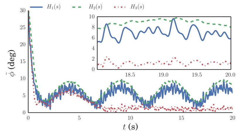
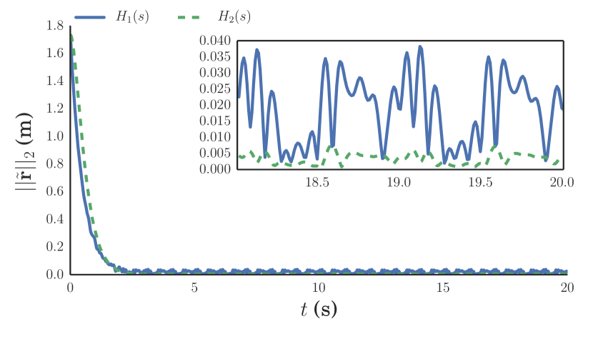
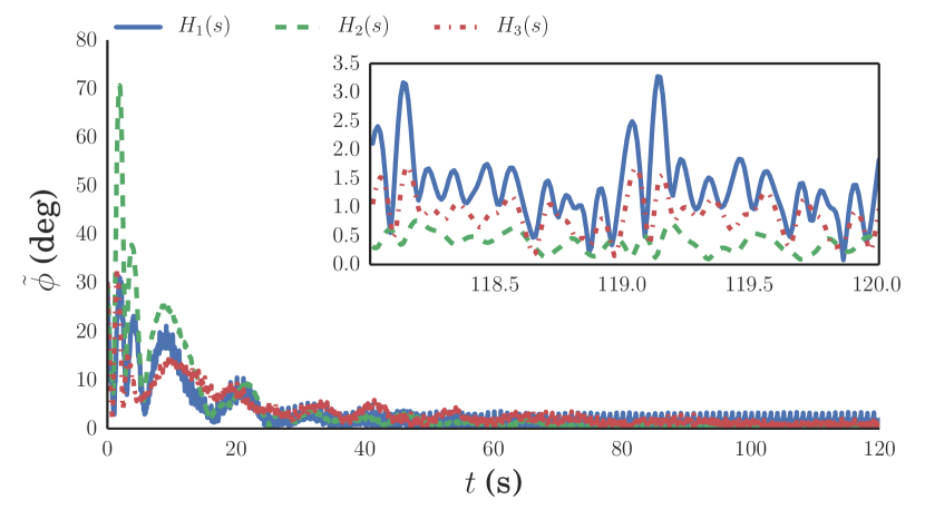
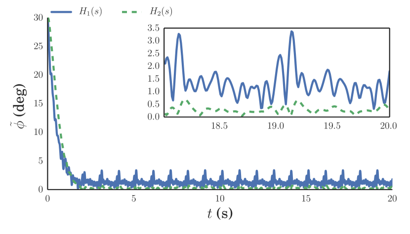
The multiplicative noise associated with the reference vector measurements, 𝐍𝐣=exp(𝐒(𝐧𝐣))subscript𝐍𝐣𝐒subscript𝐧𝐣\mbf{N}_{j}=\exp(S(\mbf{n}_{j})), are constructed by selecting 𝐧𝐣subscript𝐧𝐣\mbf{n}_{j} as linear combinations of harmonic signals with frequencies in the range [8π,16π]8𝜋16𝜋[8\pi,16\pi] (rad/s) and amplitudes in the range [0.05,0.4]0.050.4[0.05,0.4]. The undesirable effects of 𝐧𝐣(𝐭)subscript𝐧𝐣𝐭\mbf{n}_{j}(t) can be mitigated by designing T(s)𝑇𝑠T(s) as a low-pass filter with an appropriate cutoff frequency. Consider two versions of H(s)𝐻𝑠H(s), H1(s)=ksubscript𝐻1𝑠𝑘H_{1}(s)=k and H2(s)=b/(s+a)subscript𝐻2𝑠𝑏𝑠𝑎H_{2}(s)=b/(s+a), where k,a,b(0,)𝑘𝑎𝑏0k,a,b\in(0,\infty). By selecting H1(s)subscript𝐻1𝑠H_{1}(s) the transfer function T(s)𝑇𝑠T(s) is a first order low-pass filter of the form T(s)=k/(s+k)𝑇𝑠𝑘𝑠𝑘T(s)=k/(s+k). This is equivalent to the pose observer proposd in [18]. Alternatively, selecting the SPR transfer function H2(s)subscript𝐻2𝑠H_{2}(s) results in a second order low-pass filter T(s)=b/(s2+as+b)𝑇𝑠𝑏superscript𝑠2𝑎𝑠𝑏T(s)=b/(s^{2}+as+b). Selecting k=2𝑘2k=2, a=6.2𝑎6.2a=6.2, and b=9.7𝑏9.7b=9.7 results in a cutoff frequency of 222 (rad/s) for T(s)𝑇𝑠T(s). Although H1(s)subscript𝐻1𝑠H_{1}(s) and H2(s)subscript𝐻2𝑠H_{2}(s) give the same cutoff frequency for T(s)𝑇𝑠T(s), the second order low-pass filter rolls off at 4040-40 dB per decade while the first order low-pass filter rolls off at 2020-20 dB per decade. Consequently, it is expected that greater noise mitigation can be accomplished by selecting H2(s)subscript𝐻2𝑠H_{2}(s) over H1(s)subscript𝐻1𝑠H_{1}(s). Simulation results for the observer in (17) with both H1(s)subscript𝐻1𝑠H_{1}(s) and H2(s)subscript𝐻2𝑠H_{2}(s) are shown in Fig. 2(a). Referring to Fig. 2(a), the steady state error associated with the SPR filter H2(s)subscript𝐻2𝑠H_{2}(s) is indeed lower than that with a constant transfer function, as was expected. This indicates that superior noise mitigation is possible with the appropriate selection of an SPR filter.

Case 2 (input disturbance)

Suppose now that in addition to partial state measurement noise, the velocity measurement is corrupted by harmonic disturbances. Specifically, let 𝐰(𝐭)=[𝐰𝟏(𝐭)𝐰𝟐(𝐭)𝐰𝟑(𝐭)𝐰𝟒(𝐭)𝐰𝟓(𝐭)𝐰𝟔(𝐭)]𝖳𝐰𝐭superscriptdelimited-[]subscript𝐰1𝐭subscript𝐰2𝐭subscript𝐰3𝐭subscript𝐰4𝐭subscript𝐰5𝐭subscript𝐰6𝐭𝖳\mbf{w}(t)=[\ w_{1}(t)\ w_{2}(t)\ w_{3}(t)\ w_{4}(t)\ w_{5}(t)\ w_{6}(t)\ ]^{\mathsf{T}} be composed of harmonic signals such that

wi(t)=αisin(0.2πt)+βicos(0.2πt),i=1,,6,formulae-sequencesubscript𝑤𝑖𝑡subscript𝛼𝑖0.2𝜋𝑡subscript𝛽𝑖0.2𝜋𝑡for-all𝑖16w_{i}(t)=\alpha_{i}\sin(0.2\pi t)+\beta_{i}\cos(0.2\pi t),\ \forall i=1,\ldots,6, (20)

where αi,βi[0.1,0.2]subscript𝛼𝑖subscript𝛽𝑖0.10.2\alpha_{i},\beta_{i}\in[0.1,0.2] and αisubscript𝛼𝑖\alpha_{i} and βisubscript𝛽𝑖\beta_{i} have appropriate units. A simple method to mitigate the effect of 𝐰𝐰\mbf{w} is to add a notch filter at 0.2π0.2𝜋0.2\pi (rad/s) to S(s)𝑆𝑠S(s). In this way, the gain of S(s)𝑆𝑠S(s) at 0.2π0.2𝜋0.2\pi (rad/s) can be significantly reduced thereby attenuating 𝐰𝐰\mbf{w}. Let M(s)=(s2+0.1s+(0.2π)2)/(s2+s+(0.2π)2)𝑀𝑠superscript𝑠20.1𝑠superscript0.2𝜋2superscript𝑠2𝑠superscript0.2𝜋2M(s)=(s^{2}+0.1s+(0.2\pi)^{2})/(s^{2}+s+(0.2\pi)^{2}) be the notch filter, and consider a third version of H(s)𝐻𝑠H(s), denoted H3(s)subscript𝐻3𝑠H_{3}(s). The filter H3(s)subscript𝐻3𝑠H_{3}(s) is designed by letting S3(s)=S2(s)M(s)subscript𝑆3𝑠subscript𝑆2𝑠𝑀𝑠S_{3}(s)=S_{2}(s)M(s), where S2(s)=s/(s+H2(s))subscript𝑆2𝑠𝑠𝑠subscript𝐻2𝑠S_{2}(s)=s/(s+H_{2}(s)), and solving for H3(s)subscript𝐻3𝑠H_{3}(s) by S3(s)=s/(s+H3(s))subscript𝑆3𝑠𝑠𝑠subscript𝐻3𝑠S_{3}(s)=s/(s+H_{3}(s)). Employing this method yields

H3(s)subscript𝐻3𝑠\displaystyle H_{3}(s) =\displaystyle= 0.9s3+15.25s2+9.7s+3.8s3+6.3s2+1.0s+2.450.9superscript𝑠315.25superscript𝑠29.7𝑠3.8superscript𝑠36.3superscript𝑠21.0𝑠2.45\displaystyle\frac{0.9s^{3}+15.25s^{2}+9.7s+3.8}{s^{3}+6.3s^{2}+1.0s+2.45}
=\displaystyle= 9.6s2+8.7s+1.6s3+6.315s2+1.0s+2.45+0.99.6superscript𝑠28.7𝑠1.6superscript𝑠36.315superscript𝑠21.0𝑠2.450.9\displaystyle\frac{9.6s^{2}+8.7s+1.6}{s^{3}+6.315s^{2}+1.0s+2.45}+0.9
=\displaystyle= Hspr(s)+D,subscript𝐻𝑠𝑝𝑟𝑠𝐷\displaystyle H_{spr}(s)+D,

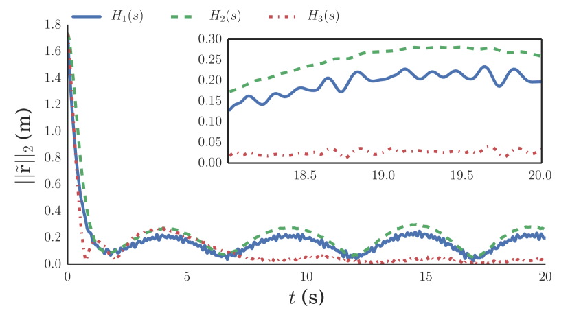
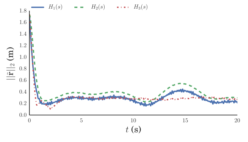
where it can be shown that Hspr(s)subscript𝐻𝑠𝑝𝑟𝑠H_{spr}(s) is SPR. Simulation results for H1(s)subscript𝐻1𝑠H_{1}(s), H2(s)subscript𝐻2𝑠H_{2}(s), and H3(s)subscript𝐻3𝑠H_{3}(s) are shown in Fig. 2(b). The steady state performance of (17) with both H1(s)subscript𝐻1𝑠H_{1}(s) and H2(s)subscript𝐻2𝑠H_{2}(s) observed in case 1 has been lost. However, the results indicate that the inclusion of the notch filter in H3(s)subscript𝐻3𝑠H_{3}(s) is successful in mitigating the effects of the input disturbance. If in addition to harmonic disturbances a constant bias is added to 𝐰𝐰\mbf{w} such that

wi(t)=αisin(0.2πt)+βicos(0.2πt)+bi,i=1,,6,formulae-sequencesubscript𝑤𝑖𝑡subscript𝛼𝑖0.2𝜋𝑡subscript𝛽𝑖0.2𝜋𝑡subscript𝑏𝑖for-all𝑖16w_{i}(t)=\alpha_{i}\sin(0.2\pi t)+\beta_{i}\cos(0.2\pi t)+b_{i},\ \forall i=1,\ldots,6, (21)

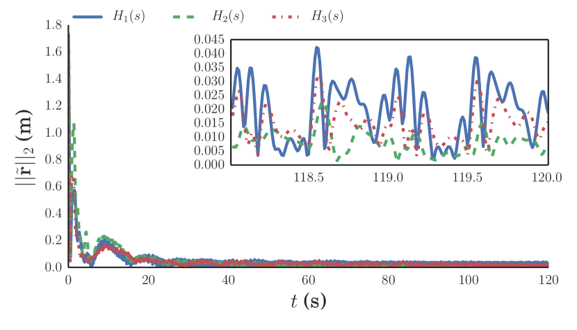
where bisubscript𝑏𝑖b_{i}\in\mathbb{R} is a constant, then the steady state performance of (17) is significantly degraded. This is shown in Fig. 2(c) where the previous simulation is repeated with bi[0.5,0.5]subscript𝑏𝑖0.50.5b_{i}\in[-0.5,0.5]. The poor performance of (17) in this case motivates the introduction of the disturbance observer discussed in Sec. IV.

Case 3 (disturbance observer)
Refer to caption
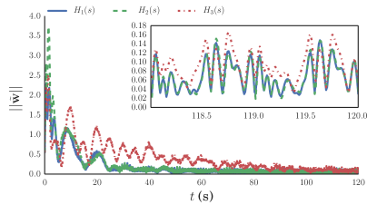
Figure 1: Error in the disturbance estimate approaches zero.

In an effort to regain the steady-state performance of the proposed observer in the presence of velocity disturbances and constant bias, the disturbance observer presented in Sec. IV is now implemented. The disturbance, 𝐰𝐰\mbf{w}, can be written as the output of the linear system in (10), where 𝐀𝐝=diag{𝐀𝟏,𝐀𝟐,𝐀𝟑,𝐀𝟒,𝐀𝟔,𝐀𝟔}subscript𝐀𝐝diagsubscript𝐀1subscript𝐀2subscript𝐀3subscript𝐀4subscript𝐀6subscript𝐀6\mbf{A}_{d}=\text{diag}\{\mbf{A}_{1},\mbf{A}_{2},\mbf{A}_{3},\mbf{A}_{4},\mbf{A}_{6},\mbf{A}_{6}\}, 𝐂𝐝=diag{𝐂𝟏,𝐂𝟐,𝐂𝟑,𝐂𝟒,𝐂𝟓,𝐂𝟔}subscript𝐂𝐝diagsubscript𝐂1subscript𝐂2subscript𝐂3subscript𝐂4subscript𝐂5subscript𝐂6\mbf{C}_{d}=\text{diag}\{\mbf{C}_{1},\mbf{C}_{2},\mbf{C}_{3},\mbf{C}_{4},\mbf{C}_{5},\mbf{C}_{6}\},

𝐀𝐢=[𝟎𝟎𝟎𝟎𝟎0.2π𝟎0.2π𝟎],𝐢=𝟏,,𝟔,formulae-sequencesubscript𝐀𝐢delimited-[]000000.2𝜋00.2𝜋0for-all𝐢16\mbf{A}_{i}=\left[\begin{array}[]{c c c}0&0&0\\ 0&0&0.2\pi\\ 0&-0.2\pi&0\end{array}\right],\ \forall i=1,\ldots,6,

and 𝐂𝐢=[ 1 1/(0.2π) 0]subscript𝐂𝐢delimited-[]110.2𝜋 0\mbf{C}_{i}=[\ 1\ 1/(0.2\pi)\ 0\ ] i=1,,6for-all𝑖16\forall i=1,\ldots,6, with appropriate initial conditions. Then, the proposed observer on SE(3)𝑆𝐸3SE(3) and the associated disturbance observer are given by

𝐓^˙˙^𝐓\displaystyle\dot{{\hat{\mbf{T}}}} =\displaystyle= 𝐓^𝐕𝐲𝐓^𝐒(𝐰^)𝐒(𝐮)𝐓^,^𝐓subscript𝐕𝐲^𝐓𝐒^𝐰𝐒𝐮^𝐓\displaystyle{\hat{\mbf{T}}}\mbf{V}_{y}-{\hat{\mbf{T}}}S({\hat{\mbf{w}}})-{S}(\mbf{u}){\hat{\mbf{T}}},
𝐱˙fsubscript˙𝐱𝑓\displaystyle\dot{\mbf{x}}_{f} =\displaystyle= 𝐀𝐟𝐱𝐟+𝐁𝐟𝐞,subscript𝐀𝐟subscript𝐱𝐟subscript𝐁𝐟𝐞\displaystyle\mbf{A}_{f}\mbf{x}_{f}+\mbf{B}_{f}\mbf{e},
𝐮𝐮\displaystyle\mbf{u} =\displaystyle= 𝐂𝐟𝐱𝐟+𝐃𝐟𝐞,subscript𝐂𝐟subscript𝐱𝐟subscript𝐃𝐟𝐞\displaystyle\mbf{C}_{f}\mbf{x}_{f}+\mbf{D}_{f}\mbf{e},
𝐱^˙dsubscript˙^𝐱𝑑\displaystyle\dot{{\hat{\mbf{x}}}}_{d} =\displaystyle= 𝐀𝐝𝐱^𝐝+ρ𝐂𝐝𝖳𝐞¯,subscript𝐀𝐝subscript^𝐱𝐝𝜌superscriptsubscript𝐂𝐝𝖳¯𝐞\displaystyle\mbf{A}_{d}{\hat{\mbf{x}}}_{d}+\rho\mbf{C}_{d}^{\mathsf{T}}{\bar{\mbf{e}}},
𝐰^^𝐰\displaystyle{\hat{\mbf{w}}} =\displaystyle= 𝐂𝐝𝐱^𝐝,subscript𝐂𝐝subscript^𝐱𝐝\displaystyle\mbf{C}_{d}{\hat{\mbf{x}}}_{d},

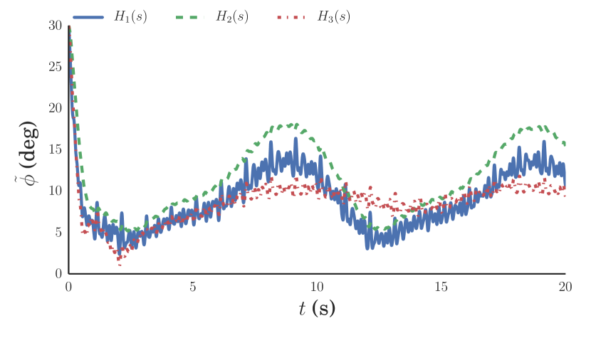
where S(𝐞¯)=𝐓^S(𝐞)𝐓^𝟏𝑆¯𝐞^𝐓𝑆𝐞superscript^𝐓1S({\bar{\mbf{e}}})={\hat{\mbf{T}}}S(\mbf{e}){\hat{\mbf{T}}}^{-1}. The results of a simulation with initial conditions (𝐓^,𝐱𝐟,𝐱^𝐝)=(𝟏,𝟎,𝟎)^𝐓subscript𝐱𝐟subscript^𝐱𝐝100({\hat{\mbf{T}}},\mbf{x}_{f},{\hat{\mbf{x}}}_{d})=(\mbf{1},\mbf{0},\mbf{0}) and ρ=0.5𝜌0.5\rho=0.5 is shown in Fig. 2(d) and Fig. 1. The pose estimation error is shown in Fig. 2(d) while the error associated with the disturbance estimate is shown in Fig. 1. Referring to Fig. 1, it can be seen that the disturbance observer is successfull in tracking the true disturbance as 𝐰~~𝐰{\tilde{\mbf{w}}} approaches zero for all observers. Consequently, the steady-state attitude error observed in Fig. 2(a) has been recovered, as shown in Fig. 2(d).
Refer to caption
Refer to caption
Refer to caption
(a) Simulation results for case 1.
Refer to caption
(b) Simulation results for case 2.
Refer to caption
Refer to caption
Refer to caption
(c) Simulation results for case 2 with constant bias.
Refer to caption
(d) Simulation results for case 3.
Figure 2: Time history of the error in the pose estimate for (a) case 1, (b) case 2, (c) case 2 with constant bias, and (d) case 3. The attitude error, ϕ~=ϕ~2~italic-ϕsubscriptnorm~bold-italic-ϕ2\tilde{\phi}=||{\tilde{\bm{\phi}}}||_{2}, and position error, 𝐫~2subscriptnorm~𝐫2||{\tilde{\mbf{r}}}||_{2}, are extracted from 𝐓~=(𝐑~,𝐫~)~𝐓~𝐑~𝐫{\tilde{\mbf{T}}}=({\tilde{\mbf{R}}},{\tilde{\mbf{r}}}), where 𝐑~=exp(ϕ~×)~𝐑superscript~bold-italic-ϕ{\tilde{\mbf{R}}}=\exp({\tilde{\bm{\phi}}}^{\times}). The steady-state error for the last two seconds is shown in the inset.

VI Conclusion

Nonlinear observer design on Lie groups has been considered. This paper builds on previously developed nonlinear observers and the proposed method is a generalization of the gradient based Lie group observer proposed in [5]. The observer has several desirable properties. First, like many recently developed nonlinear observers, the proposed method is provably locally asymptotically stable about the point at which the state estimate is equal to the true state. Secondly, the observer evolves directly on the underlying Lie group and thus captures the full nonlinear system dynamics. Third, a disturbance observer may be used to reject constant and harmonic disturbances in the velocity measurement. Finally, the introduction of an LTI system acting on the gradient of an invariant cost function allows for greater design freedom when compared to similar observers in the literature. Classical control techniques can be used to shape the sensitivity and complementary sensitivity transfer matrices of the linearized closed-loop system based on specific sensor noise characteristics. A numerical example demonstrated that the proposed observer performs admirably in the context of rigid-body pose estimation.

Appendix A Proof of Theorem 1

The proof of Theorem 1 requires the following lemma and corollary.

Lemma 1 (Kalman-Yakubovich-Popov (KYP) Lemma [32]).

Consider the LTI system

𝐱˙fsubscript˙𝐱𝑓\displaystyle\dot{\mbf{x}}_{f} =\displaystyle= 𝐀𝐟𝐱𝐟+𝐁𝐟𝐮𝐟,subscript𝐀𝐟subscript𝐱𝐟subscript𝐁𝐟subscript𝐮𝐟\displaystyle\mbf{A}_{f}\mbf{x}_{f}+\mbf{B}_{f}\mbf{u}_{f},
𝐲𝐟subscript𝐲𝐟\displaystyle\mbf{y}_{f} =\displaystyle= 𝐂𝐟𝐱𝐟,subscript𝐂𝐟subscript𝐱𝐟\displaystyle\mbf{C}_{f}\mbf{x}_{f},

where 𝐱𝐟𝐧𝐟subscript𝐱𝐟superscriptsubscript𝐧𝐟\mbf{x}_{f}\in\mathbb{R}^{n_{f}}, 𝐮𝐟,𝐲𝐟𝐦𝐟subscript𝐮𝐟subscript𝐲𝐟superscriptsubscript𝐦𝐟\mbf{u}_{f},\mbf{y}_{f}\in\mathbb{R}^{m_{f}}, and 𝐀𝐟subscript𝐀𝐟\mbf{A}_{f}, 𝐁𝐟subscript𝐁𝐟\mbf{B}_{f}, and 𝐂𝐟subscript𝐂𝐟\mbf{C}_{f} are appropriately dimensioned real matrices that form a minimal state-space realization. Moreover, assume that 𝐀𝐟subscript𝐀𝐟\mbf{A}_{f} is Hurwitz. Then, the system is strictly positive real (SPR) if and only if there exists symmetric positive definite matrices 𝐏𝐟,𝐐𝐟𝐧𝐟×𝐧𝐟subscript𝐏𝐟subscript𝐐𝐟superscriptsubscript𝐧𝐟subscript𝐧𝐟\mbf{P}_{f},\mbf{Q}_{f}\in\mathbb{R}^{n_{f}\times n_{f}} such that

𝐏𝐟𝐀𝐟+𝐀𝐟𝖳𝐏𝐟subscript𝐏𝐟subscript𝐀𝐟superscriptsubscript𝐀𝐟𝖳subscript𝐏𝐟\displaystyle\mbf{P}_{f}\mbf{A}_{f}+\mbf{A}_{f}^{\mathsf{T}}\mbf{P}_{f} =\displaystyle= 𝐐𝐟subscript𝐐𝐟\displaystyle-\mbf{Q}_{f} (23a)
𝐏𝐟𝐁𝐟subscript𝐏𝐟subscript𝐁𝐟\displaystyle\mbf{P}_{f}\mbf{B}_{f} =\displaystyle= 𝐂𝐟𝖳.superscriptsubscript𝐂𝐟𝖳\displaystyle\mbf{C}_{f}^{\mathsf{T}}. (23b)
Corollary 1.

Consider an LTI system with minimal state-space realization given by

𝐱˙fsubscript˙𝐱𝑓\displaystyle\dot{\mbf{x}}_{f} =\displaystyle= 𝐀𝐟𝐱𝐟+𝐁𝐟𝐮𝐟,subscript𝐀𝐟subscript𝐱𝐟subscript𝐁𝐟subscript𝐮𝐟\displaystyle\mbf{A}_{f}\mbf{x}_{f}+\mbf{B}_{f}\mbf{u}_{f}, (24a)
𝐲𝐟subscript𝐲𝐟\displaystyle\mbf{y}_{f} =\displaystyle= 𝐂𝐟𝐱𝐟+𝐃𝐟𝐮𝐟,subscript𝐂𝐟subscript𝐱𝐟subscript𝐃𝐟subscript𝐮𝐟\displaystyle\mbf{C}_{f}\mbf{x}_{f}+\mbf{D}_{f}\mbf{u}_{f}, (24b)

and define (𝐱𝐟)=12𝐱𝐟𝖳𝐏𝐟𝐱𝐟subscript𝐱𝐟12superscriptsubscript𝐱𝐟𝖳subscript𝐏𝐟subscript𝐱𝐟\mathcal{L}(\mbf{x}_{f})=\mbox{$\textstyle{\frac{1}{2}}$}\mbf{x}_{f}^{\mathsf{T}}\mbf{P}_{f}\mbf{x}_{f}. If matrices (𝐀𝐟,𝐁𝐟,𝐂𝐟)subscript𝐀𝐟subscript𝐁𝐟subscript𝐂𝐟(\mbf{A}_{f},\mbf{B}_{f},\mbf{C}_{f}) satisfy the KYP equations (23) then, regardless of the choice of 𝐃𝐟subscript𝐃𝐟\mbf{D}_{f}, the time derivative of \mathcal{L} is given by

˙(𝐱𝐟)=12𝐱𝐟𝖳𝐐𝐟𝐱𝐟+𝐮𝐟𝖳𝐲𝐟𝐮𝐟𝖳𝐃𝐟𝐮𝐟.˙subscript𝐱𝐟12superscriptsubscript𝐱𝐟𝖳subscript𝐐𝐟subscript𝐱𝐟superscriptsubscript𝐮𝐟𝖳subscript𝐲𝐟superscriptsubscript𝐮𝐟𝖳subscript𝐃𝐟subscript𝐮𝐟\dot{\mathcal{L}}(\mbf{x}_{f})=-\mbox{$\textstyle{\frac{1}{2}}$}\mbf{x}_{f}^{\mathsf{T}}\mbf{Q}_{f}\mbf{x}_{f}+\mbf{u}_{f}^{\mathsf{T}}\mbf{y}_{f}-\mbf{u}_{f}^{\mathsf{T}}\mbf{D}_{f}\mbf{u}_{f}.

Proof The proof follows directly from equations (23) and (24). \Box

Now a proof of Theorem 1 is given, starting with item (i) in Theorem 1. Consider the Lyapunov function candidate

V1(X~,𝐱𝐟)=𝐟(𝐗~,𝐈)+(𝐱𝐟).subscript𝑉1~𝑋subscript𝐱𝐟𝐟~𝐗𝐈subscript𝐱𝐟V_{1}(\tilde{X},\mbf{x}_{f})=f(\tilde{X},I)+\mathcal{L}(\mbf{x}_{f}). (25)

The derivative with respect to time of V1subscript𝑉1V_{1} is

V˙1(X~,𝐱𝐟)subscript˙𝑉1~𝑋subscript𝐱𝐟\displaystyle\dot{V}_{1}(\tilde{X},\mbf{x}_{f}) =\displaystyle= X~fI(X~),X~˙X~+˙(𝐱𝐟)subscriptsubscript~𝑋subscript𝑓𝐼~𝑋˙~𝑋~𝑋˙subscript𝐱𝐟\displaystyle\langle{\nabla}_{\tilde{X}}f_{I}(\tilde{X}),\dot{\tilde{X}}\rangle_{\tilde{X}}+\dot{\mathcal{L}}(\mbf{x}_{f})
=\displaystyle= S(𝐞)𝐗~,𝐒(𝐮)𝐗~𝐗~+˙(𝐱𝐟)subscript𝑆𝐞~𝐗𝐒𝐮~𝐗~𝐗˙subscript𝐱𝐟\displaystyle-\langle S(\mbf{e})\tilde{X},S(\mbf{u})\tilde{X}\rangle_{\tilde{X}}+\dot{\mathcal{L}}(\mbf{x}_{f})
=\displaystyle= S(𝐞),𝐒(𝐮)+˙(𝐱𝐟)𝑆𝐞𝐒𝐮˙subscript𝐱𝐟\displaystyle-\langle S(\mbf{e}),S(\mbf{u})\rangle+\dot{\mathcal{L}}(\mbf{x}_{f})
=\displaystyle= 𝐞𝖳𝐮+˙(𝐱𝐟).superscript𝐞𝖳𝐮˙subscript𝐱𝐟\displaystyle-\mbf{e}^{\mathsf{T}}\mbf{u}+\dot{\mathcal{L}}(\mbf{x}_{f}).

By application of Corollary 1, V˙1subscript˙𝑉1\dot{V}_{1} is given by

V˙1(X~,𝐱𝐟)=𝐞𝖳𝐮12𝐱𝐟𝖳𝐐𝐟𝐱𝐟+𝐞𝖳𝐮𝐞𝖳𝐃𝐟𝐞.subscript˙𝑉1~𝑋subscript𝐱𝐟superscript𝐞𝖳𝐮12superscriptsubscript𝐱𝐟𝖳subscript𝐐𝐟subscript𝐱𝐟superscript𝐞𝖳𝐮superscript𝐞𝖳subscript𝐃𝐟𝐞\dot{V}_{1}(\tilde{X},\mbf{x}_{f})=-\mbf{e}^{\mathsf{T}}\mbf{u}-\mbox{$\textstyle{\frac{1}{2}}$}\mbf{x}_{f}^{\mathsf{T}}\mbf{Q}_{f}\mbf{x}_{f}+\mbf{e}^{\mathsf{T}}\mbf{u}-\mbf{e}^{\mathsf{T}}\mbf{D}_{f}\mbf{e}.

Consequently, V˙1(X~,𝐱𝐟)=12𝐱𝐟𝖳𝐐𝐟𝐱𝐟𝐞𝖳𝐃𝐟𝐞subscript˙𝑉1~𝑋subscript𝐱𝐟12superscriptsubscript𝐱𝐟𝖳subscript𝐐𝐟subscript𝐱𝐟superscript𝐞𝖳subscript𝐃𝐟𝐞\dot{V}_{1}(\tilde{X},\mbf{x}_{f})=-\mbox{$\textstyle{\frac{1}{2}}$}\mbf{x}_{f}^{\mathsf{T}}\mbf{Q}_{f}\mbf{x}_{f}-\mbf{e}^{\mathsf{T}}\mbf{D}_{f}\mbf{e}. By assumption 𝐃𝐟𝟎subscript𝐃𝐟0\mbf{D}_{f}\geq 0, which implies V˙1(X~,𝐱𝐟)12𝐱𝐟𝖳𝐐𝐟𝐱𝐟subscript˙𝑉1~𝑋subscript𝐱𝐟12superscriptsubscript𝐱𝐟𝖳subscript𝐐𝐟subscript𝐱𝐟\dot{V}_{1}(\tilde{X},\mbf{x}_{f})\leq-\mbox{$\textstyle{\frac{1}{2}}$}\mbf{x}_{f}^{\mathsf{T}}\mbf{Q}_{f}\mbf{x}_{f} and thus V˙1(X~,𝐱𝐟)𝟎subscript˙𝑉1~𝑋subscript𝐱𝐟0\dot{V}_{1}(\tilde{X},\mbf{x}_{f})\leq 0 and V1(X~(t),𝐱𝐟(𝐭))𝐕𝟏(𝐗~(𝟎),𝐱𝐟(𝟎))subscript𝑉1~𝑋𝑡subscript𝐱𝐟𝐭subscript𝐕1~𝐗0subscript𝐱𝐟0V_{1}(\tilde{X}(t),\mbf{x}_{f}(t))\leq V_{1}(\tilde{X}(0),\mbf{x}_{f}(0)) for all t0𝑡0t\geq 0. By Remark 11.11 of [1], f𝑓f is locally positive definite and X~=I~𝑋𝐼\tilde{X}=I is an isolated critical point of f𝑓f. By assumption, there exists a faithful representation of G𝐺G as a matrix Lie group. This implies that there exists m>0𝑚0m>0 and a mapping 𝚽:GGL(m):𝚽𝐺𝐺𝐿𝑚{\bm{\Phi}}:G\rightarrow GL(m) such that 𝚽(G)𝚽𝐺{\bm{\Phi}}(G) is a matrix Lie group [7]. Following the proof of Theorem 5.1 in [7], this implies that there exists a set Br={X~G|d(X~)r}subscript𝐵𝑟conditional-set~𝑋𝐺𝑑~𝑋𝑟B_{r}=\{\tilde{X}\in G\ |\ d(\tilde{X})\leq r\} about X~=I~𝑋𝐼\tilde{X}=I, where d(X~)=𝟏𝚽(𝐗~)𝖥𝑑~𝑋subscriptnorm1𝚽~𝐗𝖥d(\tilde{X})=||\mbf{1}-{\bm{\Phi}}(\tilde{X})||_{\mathsf{F}}, such that for all X~Br~𝑋subscript𝐵𝑟\tilde{X}\in B_{r}, f(X~,I)𝑓~𝑋𝐼f(\tilde{X},I) is positive definite and X~=I~𝑋𝐼\tilde{X}=I is the only critical point of f𝑓f in Brsubscript𝐵𝑟B_{r}. Further, this implies that V1(X~,𝐱𝐟)subscript𝑉1~𝑋subscript𝐱𝐟V_{1}(\tilde{X},\mbf{x}_{f}) is positive definite in the set B¯r={(X~,𝐱𝐟)𝐆×𝐧𝐟|(𝐗~,𝐱𝐟)𝐫}subscript¯𝐵𝑟conditional-set~𝑋subscript𝐱𝐟𝐆superscriptsubscript𝐧𝐟~𝐗subscript𝐱𝐟𝐫\bar{B}_{r}=\{(\tilde{X},\mbf{x}_{f})\in G\times\mathbb{R}^{n_{f}}\ |\ \ell(\tilde{X},\mbf{x}_{f})\leq r\}, where (X~,𝐱𝐟)=𝐝(𝐗~)+𝐱𝐟𝟐~𝑋subscript𝐱𝐟𝐝~𝐗subscriptnormsubscript𝐱𝐟2\ell(\tilde{X},\mbf{x}_{f})=d(\tilde{X})+||\mbf{x}_{f}||_{2}, and X~=I~𝑋𝐼\tilde{X}=I is the only critical point of f𝑓f in B¯rsubscript¯𝐵𝑟\bar{B}_{r}.

A corollary to LaSalle’s invariant set theorem will now be used to prove local asymptotic stability [33, p. 128]. Let 𝒮={(X~,𝐱𝐟)𝐁¯𝐫|𝐕˙𝟏(𝐗~,𝐱𝐟)=𝟎}𝒮conditional-set~𝑋subscript𝐱𝐟subscript¯𝐁𝐫subscript˙𝐕1~𝐗subscript𝐱𝐟0\mathcal{S}=\{(\tilde{X},\mbf{x}_{f})\in\bar{B}_{r}\ |\ \dot{V}_{1}(\tilde{X},\mbf{x}_{f})=0\}. It will now be shown that the only solution that can stay identically in 𝒮𝒮\mathcal{S} is the solution (X~,𝐱𝐟)=(𝐈,𝟎)~𝑋subscript𝐱𝐟𝐈0(\tilde{X},\mbf{x}_{f})=(I,\mbf{0}). For all (X~,𝐱𝐟)𝒮~𝑋subscript𝐱𝐟𝒮(\tilde{X},\mbf{x}_{f})\in\mathcal{S}, 𝐱𝐟𝟎subscript𝐱𝐟0\mbf{x}_{f}\equiv\mbf{0}. With 𝐱𝐟𝟎subscript𝐱𝐟0\mbf{x}_{f}\equiv\mbf{0}, it follows that 𝐱˙f𝟎subscript˙𝐱𝑓0\dot{\mbf{x}}_{f}\equiv\mbf{0}. This implies that 𝐁𝐟𝐞𝟎subscript𝐁𝐟𝐞0\mbf{B}_{f}\mbf{e}\equiv\mbf{0}. Since 𝐁𝐟subscript𝐁𝐟\mbf{B}_{f} has full rank by assumption, 𝐁𝐟𝐞𝟎subscript𝐁𝐟𝐞0\mbf{B}_{f}\mbf{e}\equiv\mbf{0} implies that 𝐞𝟎𝐞0\mbf{e}\equiv\mbf{0} and consequently X~fI(X~)0subscript~𝑋subscript𝑓𝐼~𝑋0{\nabla}_{\tilde{X}}f_{I}(\tilde{X})\equiv 0. As the only critical point of f𝑓f in B¯rsubscript¯𝐵𝑟\bar{B}_{r} is the point X~=I~𝑋𝐼\tilde{X}=I, it follows that X~fI(X~)0subscript~𝑋subscript𝑓𝐼~𝑋0{\nabla}_{\tilde{X}}f_{I}(\tilde{X})\equiv 0 implies X~=I~𝑋𝐼\tilde{X}=I. Thus, by Corollary 4.1 of [33, p. 128] the equilibrium point (X~,𝐱𝐟)=(𝐈,𝟎)~𝑋subscript𝐱𝐟𝐈0(\tilde{X},\mbf{x}_{f})=(I,\mbf{0}) is locally asymptotically stable. This proves item (i).

The following corollary will be required for the proof of item (ii).

Corollary 2.

Consider the gradient vector field fI(X~)=S(𝐞)𝐗~subscript𝑓𝐼~𝑋𝑆𝐞~𝐗{\nabla}f_{I}(\tilde{X})=S(\mbf{e})\tilde{X} and let X~˙=S(𝐪)𝐗~˙~𝑋𝑆𝐪~𝐗\dot{\tilde{X}}=S(\mbf{q})\tilde{X}, where 𝐪𝐧𝐪superscript𝐧\mbf{q}\in\mathbb{R}^{n}. Then, the derivative with respect to time of 𝐞𝐞\mbf{e} is given by

𝐞˙=𝐇(𝐗~)𝐪𝝃,˙𝐞𝐇~𝐗𝐪𝝃\dot{\mbf{e}}=\mbf{H}(\tilde{X})\mbf{q}-{\bm{\xi}},

where 𝐇(𝐗~)𝐇~𝐗\mbf{H}(\tilde{X}) is the matrix representation in basis BX~subscript𝐵~𝑋B_{\tilde{X}} of the Riemannian Hessian operator HfI(X~)()subscript𝐻subscript𝑓𝐼~𝑋H_{f_{I}(\tilde{X})}(\cdot) at point X~~𝑋\tilde{X}, and 𝝃n𝝃superscript𝑛{\bm{\xi}}\in\mathbb{R}^{n}. Moreover, there exists a finite constant m<𝑚m<\infty such that 𝝃𝝃{\bm{\xi}} satisfies 𝝃2m𝐪𝟐𝐞𝟐subscriptnorm𝝃2𝑚subscriptnorm𝐪2subscriptnorm𝐞2||{\bm{\xi}}||_{2}\leq m||\mbf{q}||_{2}||\mbf{e}||_{2}.

Proof Let X~~𝑋\tilde{X} be a trajectory under the ordinary differential equation X~˙=S(𝐪)𝐗~˙~𝑋𝑆𝐪~𝐗\dot{\tilde{X}}=S(\mbf{q})\tilde{X}, and consider the gradient vector field fI(X~)subscript𝑓𝐼~𝑋{\nabla}f_{I}(\tilde{X}). Let ΓΓ\Gamma be a vector field along the curve X~~𝑋\tilde{X} such that Γ(t)=fI(X~(t))Γ𝑡subscript𝑓𝐼~𝑋𝑡\Gamma(t)={\nabla}f_{I}(\tilde{X}(t)). The covariant derivative of ΓΓ\Gamma along X~~𝑋\tilde{X} is given by [1, p. 139],

DΓdt=S(𝐞˙)X~+Q(S(𝐪),𝐒(𝐞))𝐗~,DΓd𝑡𝑆˙𝐞~𝑋𝑄𝑆𝐪𝐒𝐞~𝐗\frac{\mathrm{D}\Gamma}{\mathrm{d}t}=S(\dot{\mbf{e}})\tilde{X}+Q(S(\mbf{q}),S(\mbf{e}))\tilde{X}, (26)

where Q:𝔤×𝔤𝔤:𝑄𝔤𝔤𝔤Q:\mathfrak{g}\times\mathfrak{g}\rightarrow\mathfrak{g} is the unique bilinear mapping associated with the Levi-Civita connection such that for any two right invariant vector fields V(X)=vX𝑉𝑋𝑣𝑋V(X)=vX and U(X)=uX𝑈𝑋𝑢𝑋U(X)=uX, VU=Q(v,u)Xsubscript𝑉𝑈𝑄𝑣𝑢𝑋\nabla_{V}U=Q(v,u)X. By definition the covariant derivative satisfies

DΓdt=X~˙fI(X~),DΓd𝑡subscript˙~𝑋subscript𝑓𝐼~𝑋\frac{\mathrm{D}\Gamma}{\mathrm{d}t}={\nabla}_{\dot{\tilde{X}}}{\nabla}f_{I}(\tilde{X}),

and from the definition of the Hessian operator in (2) it follows that

DΓdt=HfI(X~)(X~˙).DΓd𝑡subscript𝐻subscript𝑓𝐼~𝑋˙~𝑋\frac{\mathrm{D}\Gamma}{\mathrm{d}t}=H_{f_{I}(\tilde{X})}(\dot{\tilde{X}}). (27)

Combining (26) and (27) yields

S(𝐞˙)X~=HfI(X~)(X~˙)Q(S(𝐪),𝐒(𝐞))𝐗~.𝑆˙𝐞~𝑋subscript𝐻subscript𝑓𝐼~𝑋˙~𝑋𝑄𝑆𝐪𝐒𝐞~𝐗S(\dot{\mbf{e}})\tilde{X}=H_{f_{I}(\tilde{X})}(\dot{\tilde{X}})-Q(S(\mbf{q}),S(\mbf{e}))\tilde{X}. (28)

Resolving (28) in basis BX~subscript𝐵~𝑋B_{\tilde{X}} yields

𝐞˙=𝐇(𝐗~)𝐪𝝃,˙𝐞𝐇~𝐗𝐪𝝃\dot{\mbf{e}}=\mbf{H}(\tilde{X})\mbf{q}-{\bm{\xi}},

where S(𝝃)=Q(S(𝐪),𝐒(𝐞))𝑆𝝃𝑄𝑆𝐪𝐒𝐞S({\bm{\xi}})=Q(S(\mbf{q}),S(\mbf{e})). Recall that the Riemannian manifold under consideration, namely (G,,X)𝐺subscript𝑋(G,\langle\cdot,\cdot\rangle_{X}), is a smooth Riemannian manifold. This implies that the Levi-Civita connection is continuous [1, p.115 Theorem 3.104]. This further implies that the bilinear map Q(,)𝑄Q(\cdot,\cdot) is continuous and consequently Q(,)𝑄Q(\cdot,\cdot) is bounded, which is to say that there exists m<𝑚m<\infty such that Q(a,b)𝔤ma𝔤b𝔤subscriptnorm𝑄𝑎𝑏𝔤𝑚subscriptnorm𝑎𝔤subscriptnorm𝑏𝔤||Q(a,b)||_{\mathfrak{g}}\leq m||a||_{\mathfrak{g}}||b||_{\mathfrak{g}} for all a,b𝔤𝑎𝑏𝔤a,b\in\mathfrak{g}. Thus, S(𝝃)𝔤mS(𝐪)𝔤𝐒(𝐞)𝔤subscriptnorm𝑆𝝃𝔤𝑚subscriptnorm𝑆𝐪𝔤subscriptnorm𝐒𝐞𝔤||S({\bm{\xi}})||_{\mathfrak{g}}\leq m||S(\mbf{q})||_{\mathfrak{g}}||S(\mbf{e})||_{\mathfrak{g}}, which implies that 𝝃2m𝐪𝟐𝐞𝟐subscriptnorm𝝃2𝑚subscriptnorm𝐪2subscriptnorm𝐞2||{\bm{\xi}}||_{2}\leq m||\mbf{q}||_{2}||\mbf{e}||_{2}. \Box

The proof of item (ii) in Theorem 1 continues as follows. By Corollary 6.29 of [1] there exists a constant c>0𝑐0c>0 such that the set Ωc={X~G|fI(X~)c}subscriptΩ𝑐conditional-set~𝑋𝐺subscript𝑓𝐼~𝑋𝑐\Omega_{c}=\{\tilde{X}\in G\ |\ f_{I}(\tilde{X})\leq c\} is compact and the only critical point of f𝑓f in ΩcsubscriptΩ𝑐\Omega_{c} is the point X~=I~𝑋𝐼\tilde{X}=I. By Proposition 6.30 of [1], for all c(0,L)𝑐0𝐿c\in(0,L) there exists constants 0<b1b20subscript𝑏1subscript𝑏20<b_{1}\leq b_{2} such that

b1𝐞𝟐𝟐𝐟(𝐗^,𝐗)𝐛𝟐𝐞𝟐𝟐.subscript𝑏1superscriptsubscriptnorm𝐞22𝐟^𝐗𝐗subscript𝐛2superscriptsubscriptnorm𝐞22b_{1}||\mbf{e}||_{2}^{2}\leq f(\hat{X},X)\leq b_{2}||\mbf{e}||_{2}^{2}. (29)

Consider again the function V1subscript𝑉1V_{1} given in (25) and recall that V˙10subscript˙𝑉10\dot{V}_{1}\leq 0. Therefore, V1(X~(t),𝐱𝐟(𝐭))𝐕𝟏(𝐗~(𝟎),𝐱𝐟(𝟎))subscript𝑉1~𝑋𝑡subscript𝐱𝐟𝐭subscript𝐕1~𝐗0subscript𝐱𝐟0V_{1}(\tilde{X}(t),\mbf{x}_{f}(t))\leq V_{1}(\tilde{X}(0),\mbf{x}_{f}(0)) t0for-all𝑡0\forall t\geq 0. Let V1(X~(0),𝐱𝐟(𝟎))𝐜subscript𝑉1~𝑋0subscript𝐱𝐟0𝐜V_{1}(\tilde{X}(0),\mbf{x}_{f}(0))\leq c, where c(0,L)𝑐0𝐿c\in(0,L). Then, fI(X~(t))csubscript𝑓𝐼~𝑋𝑡𝑐f_{I}(\tilde{X}(t))\leq c t0for-all𝑡0\forall t\geq 0 and X~Ωc~𝑋subscriptΩ𝑐\tilde{X}\in\Omega_{c} t0for-all𝑡0\forall t\geq 0. This implies that (29) is satisfied for all t0𝑡0t\geq 0. Then, V1subscript𝑉1V_{1} satisfies min{b1,12λ¯(𝐏𝐟)}𝐳𝟐𝟐𝐕𝟏max{𝐛𝟐,12λ¯(𝐏𝐟)}𝐳𝟐𝟐subscript𝑏112¯𝜆subscript𝐏𝐟superscriptsubscriptnorm𝐳22subscript𝐕1subscript𝐛212¯𝜆subscript𝐏𝐟superscriptsubscriptnorm𝐳22\min\{b_{1},\mbox{$\textstyle{\frac{1}{2}}$}\underline{\lambda}(\mbf{P}_{f})\}||\mbf{z}||_{2}^{2}\leq V_{1}\leq\max\{b_{2},\mbox{$\textstyle{\frac{1}{2}}$}\bar{\lambda}(\mbf{P}_{f})\}||\mbf{z}||_{2}^{2}, where λ¯()¯𝜆\underline{\lambda}(\cdot) and λ¯()¯𝜆\bar{\lambda}(\cdot) respectively denote the maximum and minimum eigenvalues of a matrix, and 𝐳=[𝐞𝟐𝐱𝐟𝟐]𝖳𝐳superscriptdelimited-[]subscriptnorm𝐞2subscriptnormsubscript𝐱𝐟2𝖳\mbf{z}=[\ ||\mbf{e}||_{2}\ ||\mbf{x}_{f}||_{2}\ ]^{\mathsf{T}}. Thus, the fact that V1(𝐗~(t),𝐱𝐟(𝐭))𝐜subscript𝑉1~𝐗𝑡subscript𝐱𝐟𝐭𝐜V_{1}({\tilde{\mbf{X}}}(t),\mbf{x}_{f}(t))\leq c for all t0𝑡0t\geq 0 implies that 𝐞𝐞\mbf{e} and 𝐱𝐟subscript𝐱𝐟\mbf{x}_{f} are bounded for all t0𝑡0t\geq 0.

Consider the Lyapunov function candidate

V2(X~,𝐱𝐟)=𝐕𝟏(𝐗~,𝐱𝐟)𝐚𝐞𝖳𝐂𝐟𝐱𝐟,subscript𝑉2~𝑋subscript𝐱𝐟subscript𝐕1~𝐗subscript𝐱𝐟superscript𝐚𝐞𝖳subscript𝐂𝐟subscript𝐱𝐟V_{2}(\tilde{X},\mbf{x}_{f})=V_{1}(\tilde{X},\mbf{x}_{f})-a\mbf{e}^{\mathsf{T}}\mbf{C}_{f}\mbf{x}_{f}, (30)

where a(0,)𝑎0a\in(0,\infty). Let γ=𝐂𝐟𝖥𝛾subscriptnormsubscript𝐂𝐟𝖥\gamma=||\mbf{C}_{f}||_{\mathsf{F}}, then V2subscript𝑉2V_{2} satisfies 𝐳𝖳𝐖𝟏𝐳𝐕𝟐𝐳𝖳𝐖𝟐𝐳superscript𝐳𝖳subscript𝐖1𝐳subscript𝐕2superscript𝐳𝖳subscript𝐖2𝐳\mbf{z}^{\mathsf{T}}\mbf{W}_{1}\mbf{z}\leq V_{2}\leq\mbf{z}^{\mathsf{T}}\mbf{W}_{2}\mbf{z}, where

𝐖𝟏=[𝐛𝟏12𝐚γ12𝐚γ12λ¯(𝐏𝐟)],and𝐖𝟐=[𝐛𝟐12𝐚γ12𝐚γ12λ¯(𝐏𝐟)].formulae-sequencesubscript𝐖1delimited-[]subscript𝐛112𝐚𝛾12𝐚𝛾12¯𝜆subscript𝐏𝐟andsubscript𝐖2delimited-[]subscript𝐛212𝐚𝛾12𝐚𝛾12¯𝜆subscript𝐏𝐟\mbf{W}_{1}=\left[\begin{array}[]{c c}b_{1}&-\mbox{$\textstyle{\frac{1}{2}}$}a\gamma\\ -\mbox{$\textstyle{\frac{1}{2}}$}a\gamma&\mbox{$\textstyle{\frac{1}{2}}$}\underline{\lambda}(\mbf{P}_{f})\end{array}\right],\ \text{and}\ \mbf{W}_{2}=\left[\begin{array}[]{c c}b_{2}&\mbox{$\textstyle{\frac{1}{2}}$}a\gamma\\ \mbox{$\textstyle{\frac{1}{2}}$}a\gamma&\mbox{$\textstyle{\frac{1}{2}}$}\bar{\lambda}(\mbf{P}_{f})\end{array}\right].

The derivative with respect to time of V2subscript𝑉2V_{2} satisfies

V˙2subscript˙𝑉2\displaystyle\dot{V}_{2} =\displaystyle= V˙1a𝐱𝐟𝖳𝐂𝐟𝖳𝐞˙𝐚𝐞𝖳𝐂𝐟𝐱˙𝐟subscript˙𝑉1𝑎superscriptsubscript𝐱𝐟𝖳superscriptsubscript𝐂𝐟𝖳˙𝐞superscript𝐚𝐞𝖳subscript𝐂𝐟subscript˙𝐱𝐟\displaystyle\dot{V}_{1}-a\mbf{x}_{f}^{\mathsf{T}}\mbf{C}_{f}^{\mathsf{T}}\dot{\mbf{e}}-a\mbf{e}^{\mathsf{T}}\mbf{C}_{f}\dot{\mbf{x}}_{f}
\displaystyle\leq 12𝐱𝐟𝖳𝐐𝐟𝐱𝐟𝐚𝐱𝐟𝖳𝐂𝐟𝖳𝐞˙𝐚𝐞𝖳𝐂𝐟𝐱˙𝐟.12superscriptsubscript𝐱𝐟𝖳subscript𝐐𝐟subscript𝐱𝐟superscriptsubscript𝐚𝐱𝐟𝖳superscriptsubscript𝐂𝐟𝖳˙𝐞superscript𝐚𝐞𝖳subscript𝐂𝐟subscript˙𝐱𝐟\displaystyle-\mbox{$\textstyle{\frac{1}{2}}$}\mbf{x}_{f}^{\mathsf{T}}\mbf{Q}_{f}\mbf{x}_{f}-a\mbf{x}_{f}^{\mathsf{T}}\mbf{C}_{f}^{\mathsf{T}}\dot{\mbf{e}}-a\mbf{e}^{\mathsf{T}}\mbf{C}_{f}\dot{\mbf{x}}_{f}.

From Corollary 2, the derivative with respect to time of 𝐞𝐞\mbf{e} is given by 𝐞˙=𝐇(𝐗~)𝐮𝝃˙𝐞𝐇~𝐗𝐮𝝃\dot{\mbf{e}}=-\mbf{H}(\tilde{X})\mbf{u}-{\bm{\xi}}, where S(𝝃)=Q(S(𝐮),𝐒(𝐞))𝑆𝝃𝑄𝑆𝐮𝐒𝐞S({\bm{\xi}})=Q(S(\mbf{u}),S(\mbf{e})) and 𝝃2m𝐮𝟐𝐞𝟐subscriptnorm𝝃2𝑚subscriptnorm𝐮2subscriptnorm𝐞2||{\bm{\xi}}||_{2}\leq m||\mbf{u}||_{2}||\mbf{e}||_{2}. Given that 𝐱𝐟subscript𝐱𝐟\mbf{x}_{f} and 𝐞𝐞\mbf{e} are bounded, it follows that 𝐮𝐮\mbf{u} is bounded as well. As ΩcsubscriptΩ𝑐\Omega_{c} is compact it follows that the norm of 𝐇(𝐗~)𝐇~𝐗\mbf{H}(\tilde{X}) is bounded [1]. Define m1=supX~Ωc𝐇(𝐗~)𝖥subscript𝑚1subscriptsupremum~𝑋subscriptΩ𝑐subscriptnorm𝐇~𝐗𝖥m_{1}=\sup_{\tilde{X}\in\Omega_{c}}||\mbf{H}(\tilde{X})||_{\mathsf{F}}, m2=msup𝐮𝟐subscript𝑚2𝑚supremumsubscriptnorm𝐮2m_{2}=m\cdot\sup||\mbf{u}||_{2}, β=𝐃𝐟𝖥𝛽subscriptnormsubscript𝐃𝐟𝖥\beta=||\mbf{D}_{f}||_{\mathsf{F}}, and ϵ=λ¯(𝐐𝐟)italic-ϵ¯𝜆subscript𝐐𝐟\epsilon=\underline{\lambda}(\mbf{Q}_{f}). Then it can be shown that

V2˙˙subscript𝑉2\displaystyle\dot{V_{2}} \displaystyle\leq 12ϵ𝐱𝐟𝟐+𝐚𝐦𝟏γ𝟐𝐱𝐟𝟐𝟐+𝐚𝐦𝟏βγ𝐱𝐟𝟐𝐞𝟐12italic-ϵsuperscriptnormsubscript𝐱𝐟2subscript𝐚𝐦1superscript𝛾2superscriptsubscriptnormsubscript𝐱𝐟22subscript𝐚𝐦1𝛽𝛾subscriptnormsubscript𝐱𝐟2subscriptnorm𝐞2\displaystyle-\mbox{$\textstyle{\frac{1}{2}}$}\epsilon||\mbf{x}_{f}||^{2}+am_{1}\gamma^{2}||\mbf{x}_{f}||_{2}^{2}+am_{1}\beta\gamma||\mbf{x}_{f}||_{2}||\mbf{e}||_{2}
+aγm2𝐱𝐟𝟐𝐞𝟐𝐚𝐞𝖳𝐂𝐟𝐀𝐟𝐱𝐟𝑎𝛾subscript𝑚2subscriptnormsubscript𝐱𝐟2subscriptnorm𝐞2superscript𝐚𝐞𝖳subscript𝐂𝐟subscript𝐀𝐟subscript𝐱𝐟\displaystyle{+}\>a\gamma m_{2}||\mbf{x}_{f}||_{2}||\mbf{e}||_{2}-a\mbf{e}^{\mathsf{T}}\mbf{C}_{f}\mbf{A}_{f}\mbf{x}_{f}
a𝐞𝖳𝐂𝐟𝐁𝐟𝐞.𝑎superscript𝐞𝖳subscript𝐂𝐟subscript𝐁𝐟𝐞\displaystyle{-}\>a\mbf{e}^{\mathsf{T}}\mbf{C}_{f}\mbf{B}_{f}\mbf{e}.

Recall from (23b) 𝐂𝐟=𝐁𝐟𝖳𝐏𝐟subscript𝐂𝐟superscriptsubscript𝐁𝐟𝖳subscript𝐏𝐟\mbf{C}_{f}=\mbf{B}_{f}^{\mathsf{T}}\mbf{P}_{f}. Let 𝚼=𝐁𝐟𝖳𝐏𝐟𝐁𝐟𝚼superscriptsubscript𝐁𝐟𝖳subscript𝐏𝐟subscript𝐁𝐟{\bm{\Upsilon}}=\mbf{B}_{f}^{\mathsf{T}}\mbf{P}_{f}\mbf{B}_{f} and note that since 𝐁𝐟subscript𝐁𝐟\mbf{B}_{f} is assumed full rank and 𝐏𝐟>𝟎subscript𝐏𝐟0\mbf{P}_{f}>0 it follows that 𝚼>0𝚼0{\bm{\Upsilon}}>0. Define δ=𝐀𝐟𝖥𝛿subscriptnormsubscript𝐀𝐟𝖥\delta=||\mbf{A}_{f}||_{\mathsf{F}}, then

V˙2subscript˙𝑉2\displaystyle\dot{V}_{2} (12ϵam1γ2)𝐱𝐟𝟐𝟐𝐚λ¯(𝚼)𝐞𝟐𝟐absent12italic-ϵ𝑎subscript𝑚1superscript𝛾2superscriptsubscriptnormsubscript𝐱𝐟22𝐚¯𝜆𝚼superscriptsubscriptnorm𝐞22\displaystyle\leq-(\mbox{$\textstyle{\frac{1}{2}}$}\epsilon-am_{1}\gamma^{2})||\mbf{x}_{f}||_{2}^{2}-a\underline{\lambda}({\bm{\Upsilon}})||\mbf{e}||_{2}^{2}
+aγ(m2+m1β+δ)𝐱𝐟𝟐𝐞𝟐.𝑎𝛾subscript𝑚2subscript𝑚1𝛽𝛿subscriptnormsubscript𝐱𝐟2subscriptnorm𝐞2\displaystyle\phantom{{}\leq{}}+a\gamma(m_{2}+m_{1}\beta+\delta)||\mbf{x}_{f}||_{2}||\mbf{e}||_{2}. (31)

Equation (31) is equivalent to V˙2𝐳𝖳𝐖𝟑𝐳subscript˙𝑉2superscript𝐳𝖳subscript𝐖3𝐳\dot{V}_{2}\leq-\mbf{z}^{\mathsf{T}}\mbf{W}_{3}\mbf{z}, where

𝐖𝟑=[𝐚λ¯(𝚼)𝐚κ𝐚κ12ϵ𝐚𝐦𝟏γ𝟐],subscript𝐖3delimited-[]𝐚¯𝜆𝚼𝐚𝜅𝐚𝜅12italic-ϵsubscript𝐚𝐦1superscript𝛾2\mbf{W}_{3}=\left[\begin{array}[]{c c}a\underline{\lambda}({\bm{\Upsilon}})&-a\kappa\\ -a\kappa&\mbox{$\textstyle{\frac{1}{2}}$}\epsilon-am_{1}\gamma^{2}\end{array}\right],

and κ=12aγ(m2+m1β+δ)𝜅12𝑎𝛾subscript𝑚2subscript𝑚1𝛽𝛿\kappa=\mbox{$\textstyle{\frac{1}{2}}$}a\gamma(m_{2}+m_{1}\beta+\delta). It can be shown that, provided

a<min{2b1λ¯(𝐏𝐟)γ2,12ϵλ¯(𝚼)λ¯(𝚼)m1γ2+κ2},𝑎2subscript𝑏1¯𝜆subscript𝐏𝐟superscript𝛾212italic-ϵ¯𝜆𝚼¯𝜆𝚼subscript𝑚1superscript𝛾2superscript𝜅2a<\min\left\{\sqrt{\frac{2b_{1}\underline{\lambda}(\mbf{P}_{f})}{\gamma^{2}}},\frac{\mbox{$\textstyle{\frac{1}{2}}$}\epsilon\underline{\lambda}({\bm{\Upsilon}})}{\underline{\lambda}({\bm{\Upsilon}})m_{1}\gamma^{2}+\kappa^{2}}\right\},

the matrices 𝐖𝟏subscript𝐖1\mbf{W}_{1}, 𝐖𝟐subscript𝐖2\mbf{W}_{2}, and 𝐖𝟑subscript𝐖3\mbf{W}_{3} are positive definite. Therefore,

λ¯(𝐖𝟏)𝐳𝟐𝟐𝐕𝟐λ¯(𝐖𝟐)𝐳𝟐𝟐¯𝜆subscript𝐖1superscriptsubscriptnorm𝐳22subscript𝐕2¯𝜆subscript𝐖2superscriptsubscriptnorm𝐳22\displaystyle\underline{\lambda}(\mbf{W}_{1})||\mbf{z}||_{2}^{2}\leq V_{2}\leq\bar{\lambda}(\mbf{W}_{2})||\mbf{z}||_{2}^{2}
V˙2λ¯(𝐖𝟑)𝐳𝟐𝟐,subscript˙𝑉2¯𝜆subscript𝐖3superscriptsubscriptnorm𝐳22\displaystyle\dot{V}_{2}\leq-\underline{\lambda}(\mbf{W}_{3})||\mbf{z}||_{2}^{2},

which implies that

𝐳(𝐭)𝟐(λ¯(𝐖𝟏)λ¯(𝐖𝟐))12𝐳(𝟎)𝟐exp(λ¯(𝐖𝟑)𝟐λ¯(𝐖𝟐)𝐭).subscriptnorm𝐳𝐭2superscript¯𝜆subscript𝐖1¯𝜆subscript𝐖212subscriptnorm𝐳02¯𝜆subscript𝐖32¯𝜆subscript𝐖2𝐭||\mbf{z}(t)||_{2}\leq\left(\frac{\underline{\lambda}(\mbf{W}_{1})}{\bar{\lambda}(\mbf{W}_{2})}\right)^{\mbox{$\textstyle{\frac{1}{2}}$}}||\mbf{z}(0)||_{2}\exp\left(-\frac{\underline{\lambda}(\mbf{W}_{3})}{2\bar{\lambda}(\mbf{W}_{2})}t\right).

Therefore, trajectories of (𝐞𝟐,𝐱𝐟𝟐)subscriptnorm𝐞2subscriptnormsubscript𝐱𝐟2(||\mbf{e}||_{2},||\mbf{x}_{f}||_{2}) exponentially approach (0,0)00(0,0). Due to the fact that trajectories of X~~𝑋\tilde{X} remain in ΩcsubscriptΩ𝑐\Omega_{c} for all t0𝑡0t\geq 0, 𝐞𝟎𝐞0\mbf{e}\rightarrow\mbf{0} implies that X~I~𝑋𝐼\tilde{X}\rightarrow I as t𝑡t\rightarrow\infty. \Box

Appendix B Proof of Theorem 2

The proof of item (i) in Theorem 2 follows in a similar manner to the proof of Theorem 5.1 in [7]. Consider the Lyapunov function candidate

V3(X~,𝐱𝐟,𝐱~𝐝)=𝐟(𝐗~,𝟏)+(𝐱𝐟)+12ρ𝟏𝐱~𝐝𝖳𝐱~𝐝.subscript𝑉3~𝑋subscript𝐱𝐟subscript~𝐱𝐝𝐟~𝐗1subscript𝐱𝐟12superscript𝜌1superscriptsubscript~𝐱𝐝𝖳subscript~𝐱𝐝V_{3}(\tilde{X},\mbf{x}_{f},{\tilde{\mbf{x}}}_{d})=f(\tilde{X},\mbf{1})+\mathcal{L}(\mbf{x}_{f})+\mbox{$\textstyle{\frac{1}{2}}$}\rho^{-1}{\tilde{\mbf{x}}}_{d}^{\mathsf{T}}{\tilde{\mbf{x}}}_{d}. (32)

The derivative with respect to time of the third term, 12ρ1𝐱~d𝖳𝐱~d12superscript𝜌1superscriptsubscript~𝐱𝑑𝖳subscript~𝐱𝑑\mbox{$\textstyle{\frac{1}{2}}$}\rho^{-1}{\tilde{\mbf{x}}}_{d}^{\mathsf{T}}{\tilde{\mbf{x}}}_{d}, is

ddt12ρ1𝐱~d𝖳𝐱~d=12ρ1𝐱~d𝖳(𝐀𝐝𝖳+𝐀𝐝)𝐱~𝐝𝐱~𝐝𝖳𝐂𝐝𝖳𝐞¯.dd𝑡12superscript𝜌1superscriptsubscript~𝐱𝑑𝖳subscript~𝐱𝑑12superscript𝜌1superscriptsubscript~𝐱𝑑𝖳superscriptsubscript𝐀𝐝𝖳subscript𝐀𝐝subscript~𝐱𝐝superscriptsubscript~𝐱𝐝𝖳superscriptsubscript𝐂𝐝𝖳¯𝐞\frac{\mathrm{d}}{\mathrm{d}t}\mbox{$\textstyle{\frac{1}{2}}$}\rho^{-1}{\tilde{\mbf{x}}}_{d}^{\mathsf{T}}{\tilde{\mbf{x}}}_{d}=\mbox{$\textstyle{\frac{1}{2}}$}\rho^{-1}{\tilde{\mbf{x}}}_{d}^{\mathsf{T}}(\mbf{A}_{d}^{\mathsf{T}}+\mbf{A}_{d}){\tilde{\mbf{x}}}_{d}-{\tilde{\mbf{x}}}_{d}^{\mathsf{T}}\mbf{C}_{d}^{\mathsf{T}}{\bar{\mbf{e}}}.

Recall that 𝐀𝐝subscript𝐀𝐝\mbf{A}_{d} is skew-symmetric and therefore 𝐀𝐝𝖳+𝐀𝐝=𝟎superscriptsubscript𝐀𝐝𝖳subscript𝐀𝐝0\mbf{A}_{d}^{\mathsf{T}}+\mbf{A}_{d}=\mbf{0}. Consequently,

ddt12ρ1𝐱~d𝖳𝐱~d=𝐱~d𝖳𝐂𝐝𝖳𝐞¯=𝐰~𝖳𝐞¯.dd𝑡12superscript𝜌1superscriptsubscript~𝐱𝑑𝖳subscript~𝐱𝑑superscriptsubscript~𝐱𝑑𝖳superscriptsubscript𝐂𝐝𝖳¯𝐞superscript~𝐰𝖳¯𝐞\frac{\mathrm{d}}{\mathrm{d}t}\mbox{$\textstyle{\frac{1}{2}}$}\rho^{-1}{\tilde{\mbf{x}}}_{d}^{\mathsf{T}}{\tilde{\mbf{x}}}_{d}=-{\tilde{\mbf{x}}}_{d}^{\mathsf{T}}\mbf{C}_{d}^{\mathsf{T}}{\bar{\mbf{e}}}=-{\tilde{\mbf{w}}}^{\mathsf{T}}{\bar{\mbf{e}}}.

The derivative with respect to time of V3subscript𝑉3V_{3} can therefore be written as

V˙3=X~f(X~,I),X~˙X~+˙(𝐱𝐟)𝐰~𝖳𝐞¯.subscript˙𝑉3subscriptsubscript~𝑋𝑓~𝑋𝐼˙~𝑋~𝑋˙subscript𝐱𝐟superscript~𝐰𝖳¯𝐞\dot{V}_{3}=\langle{\nabla}_{\tilde{X}}f(\tilde{X},I),\dot{\tilde{X}}\rangle_{\tilde{X}}+\dot{\mathcal{L}}(\mbf{x}_{f})-{\tilde{\mbf{w}}}^{\mathsf{T}}{\bar{\mbf{e}}}. (33)

Substituting (12a) into (33) yields

V˙3subscript˙𝑉3\displaystyle\dot{V}_{3} =\displaystyle= X~f(X~,I),X~˙X~+˙(𝐱𝐟)𝐰~𝖳𝐞¯subscriptsubscript~𝑋𝑓~𝑋𝐼˙~𝑋~𝑋˙subscript𝐱𝐟superscript~𝐰𝖳¯𝐞\displaystyle\langle{\nabla}_{\tilde{X}}f(\tilde{X},I),\dot{\tilde{X}}\rangle_{\tilde{X}}+\dot{\mathcal{L}}(\mbf{x}_{f})-{\tilde{\mbf{w}}}^{\mathsf{T}}{\bar{\mbf{e}}}
=\displaystyle= S(𝐞)𝐗~,𝐗~Ad𝐗(𝐰~)𝐗~𝐒(𝐞)𝐗~,𝐒(𝐮)𝐗~𝐗~subscript𝑆𝐞~𝐗~𝐗subscriptAd𝐗~𝐰~𝐗subscript𝐒𝐞~𝐗𝐒𝐮~𝐗~𝐗\displaystyle\langle S(\mbf{e})\tilde{X},\tilde{X}{\mathrm{Ad}}_{X}(\tilde{w})\rangle_{\tilde{X}}-\langle{S}(\mbf{e})\tilde{X},{S}(\mbf{u})\tilde{X}\rangle_{\tilde{X}}
+˙(𝐱𝐟)𝐰~𝖳𝐞¯˙subscript𝐱𝐟superscript~𝐰𝖳¯𝐞\displaystyle{+}\>\dot{\mathcal{L}}(\mbf{x}_{f})-{\tilde{\mbf{w}}}^{\mathsf{T}}{\bar{\mbf{e}}}
=\displaystyle= S(𝐞),𝐒(𝐮)+𝐒(𝐞),Ad𝐗^(𝐰~)𝑆𝐞𝐒𝐮𝐒𝐞subscriptAd^𝐗~𝐰\displaystyle-\langle{S}(\mbf{e}),{S}(\mbf{u})\rangle+\langle{S}(\mbf{e}),{\mathrm{Ad}}_{\hat{X}}(\tilde{w})\rangle
+˙(𝐱𝐟)𝐰~𝖳𝐞¯˙subscript𝐱𝐟superscript~𝐰𝖳¯𝐞\displaystyle{+}\>\dot{\mathcal{L}}(\mbf{x}_{f})-{\tilde{\mbf{w}}}^{\mathsf{T}}{\bar{\mbf{e}}}
=\displaystyle= 𝐞𝖳𝐮+Ad𝐗^(𝐒(𝐞)),𝐒(𝐰~)+˙(𝐱𝐟)𝐰~𝖳𝐞¯superscript𝐞𝖳𝐮superscriptsubscriptAd^𝐗𝐒𝐞𝐒~𝐰˙subscript𝐱𝐟superscript~𝐰𝖳¯𝐞\displaystyle-\mbf{e}^{\mathsf{T}}\mbf{u}+\langle{\mathrm{Ad}}_{\hat{X}}^{*}({S}(\mbf{e})),{S}({\tilde{\mbf{w}}})\rangle+\dot{\mathcal{L}}(\mbf{x}_{f})-{\tilde{\mbf{w}}}^{\mathsf{T}}{\bar{\mbf{e}}}
=\displaystyle= 𝐞𝖳𝐮+𝐒(𝐞¯),𝐒(𝐰~)+˙(𝐱𝐟)𝐰~𝖳𝐞¯superscript𝐞𝖳𝐮𝐒¯𝐞𝐒~𝐰˙subscript𝐱𝐟superscript~𝐰𝖳¯𝐞\displaystyle-\mbf{e}^{\mathsf{T}}\mbf{u}+\langle S({\bar{\mbf{e}}}),S({\tilde{\mbf{w}}})\rangle+\dot{\mathcal{L}}(\mbf{x}_{f})-{\tilde{\mbf{w}}}^{\mathsf{T}}{\bar{\mbf{e}}}
=\displaystyle= 𝐞𝖳𝐮+𝐞¯𝖳𝐰~+˙(𝐱𝐟)𝐰~𝖳𝐞¯superscript𝐞𝖳𝐮superscript¯𝐞𝖳~𝐰˙subscript𝐱𝐟superscript~𝐰𝖳¯𝐞\displaystyle-\mbf{e}^{\mathsf{T}}\mbf{u}+{\bar{\mbf{e}}}^{\mathsf{T}}{\tilde{\mbf{w}}}+\dot{\mathcal{L}}(\mbf{x}_{f})-{\tilde{\mbf{w}}}^{\mathsf{T}}{\bar{\mbf{e}}}
=\displaystyle= 𝐞𝖳𝐮+˙(𝐱𝐟).superscript𝐞𝖳𝐮˙subscript𝐱𝐟\displaystyle-\mbf{e}^{\mathsf{T}}\mbf{u}+\dot{\mathcal{L}}(\mbf{x}_{f}).

By Corollary 1, V˙3=12𝐱𝐟𝖳𝐐𝐟𝐱𝐟𝐞𝖳𝐃𝐟𝐞subscript˙𝑉312superscriptsubscript𝐱𝐟𝖳subscript𝐐𝐟subscript𝐱𝐟superscript𝐞𝖳subscript𝐃𝐟𝐞\dot{V}_{3}=-\mbox{$\textstyle{\frac{1}{2}}$}\mbf{x}_{f}^{\mathsf{T}}\mbf{Q}_{f}\mbf{x}_{f}-\mbf{e}^{\mathsf{T}}\mbf{D}_{f}\mbf{e}. Therefore, V˙30subscript˙𝑉30\dot{V}_{3}\leq 0. As f𝑓f is an error function it follows that f𝑓f is locally positive definite and X~=I~𝑋𝐼\tilde{X}=I is an isolated critical point of f𝑓f [1]. By assumption, there exists a faithful representation of G𝐺G as a matrix Lie group. This implies that there exists m>0𝑚0m>0 and a mapping 𝚽:GGL(m):𝚽𝐺𝐺𝐿𝑚{\bm{\Phi}}:G\rightarrow GL(m) such that 𝚽(G)𝚽𝐺{\bm{\Phi}}(G) is a matrix Lie group [7]. Following the proof of Theorem 5.1 in [7], this implies that there exists a set Br={X~G|d(X~)r}subscript𝐵𝑟conditional-set~𝑋𝐺𝑑~𝑋𝑟B_{r}=\{\tilde{X}\in G\ |\ d(\tilde{X})\leq r\} about X~=I~𝑋𝐼\tilde{X}=I, where d(X~)=𝟏𝚽(𝐗~)𝖥𝑑~𝑋subscriptnorm1𝚽~𝐗𝖥d(\tilde{X})=||\mbf{1}-{\bm{\Phi}}(\tilde{X})||_{\mathsf{F}}, such that for all X~Br~𝑋subscript𝐵𝑟\tilde{X}\in B_{r}, f(X~,I)𝑓~𝑋𝐼f(\tilde{X},I) is positive definite and X~=I~𝑋𝐼\tilde{X}=I is the only critical point of f𝑓f in Brsubscript𝐵𝑟B_{r}. Further, this implies that V3(X~,𝐱𝐟,𝐱~)subscript𝑉3~𝑋subscript𝐱𝐟~𝐱V_{3}(\tilde{X},\mbf{x}_{f},{\tilde{\mbf{x}}}) is positive definite in the set B¯r={(X~,𝐱𝐟,𝐱~𝐝)𝐆×𝐧𝐟×𝐧𝐝|(𝐗~,𝐱𝐟,𝐱~𝐝)𝐫}subscript¯𝐵𝑟conditional-set~𝑋subscript𝐱𝐟subscript~𝐱𝐝𝐆superscriptsubscript𝐧𝐟superscriptsubscript𝐧𝐝~𝐗subscript𝐱𝐟subscript~𝐱𝐝𝐫\bar{B}_{r}=\{(\tilde{X},\mbf{x}_{f},{\tilde{\mbf{x}}}_{d})\in G\times\mathbb{R}^{n_{f}}\times\mathbb{R}^{n_{d}}\ |\ \ell(\tilde{X},\mbf{x}_{f},{\tilde{\mbf{x}}}_{d})\leq r\}, where (X~,𝐱𝐟,𝐱~𝐝)=𝐝(𝐗~)+𝐱𝐟𝟐+𝐱~𝐝𝟐~𝑋subscript𝐱𝐟subscript~𝐱𝐝𝐝~𝐗subscriptnormsubscript𝐱𝐟2subscriptnormsubscript~𝐱𝐝2\ell(\tilde{X},\mbf{x}_{f},{\tilde{\mbf{x}}}_{d})=d(\tilde{X})+||\mbf{x}_{f}||_{2}+||{\tilde{\mbf{x}}}_{d}||_{2}, and X~=I~𝑋𝐼\tilde{X}=I is the only critical point of f𝑓f in the set B¯rsubscript¯𝐵𝑟\bar{B}_{r}. Consequently, for all t0𝑡0t\geq 0 and all (X~,𝐱𝐟,𝐱~𝐝)𝐁¯𝐫~𝑋subscript𝐱𝐟subscript~𝐱𝐝subscript¯𝐁𝐫(\tilde{X},\mbf{x}_{f},{\tilde{\mbf{x}}}_{d})\in\bar{B}_{r} the Lyapunov function V3subscript𝑉3V_{3} is positive definite and V˙30subscript˙𝑉30\dot{V}_{3}\leq 0 and by Theorem 4.8 of [33] the equilibrium point (X~,𝐱𝐟,𝐱~𝐝)=(𝐈,𝟎,𝟎)~𝑋subscript𝐱𝐟subscript~𝐱𝐝𝐈00(\tilde{X},\mbf{x}_{f},{\tilde{\mbf{x}}}_{d})=(I,\mbf{0},\mbf{0}) is uniformly stable.

Again, following the proof of Theorem 5.1 in [7], choose α<min(X~,𝐱𝐟,𝐱~𝐝)=𝐫V3(X~,𝐱𝐟,𝐱~𝐝)𝛼subscript~𝑋subscript𝐱𝐟subscript~𝐱𝐝𝐫subscript𝑉3~𝑋subscript𝐱𝐟subscript~𝐱𝐝\alpha<\min_{\ell(\tilde{X},\mbf{x}_{f},{\tilde{\mbf{x}}}_{d})=r}V_{3}(\tilde{X},\mbf{x}_{f},{\tilde{\mbf{x}}}_{d}), and define α={(X~,𝐱𝐟,𝐱~𝐝)𝐁¯𝐫|𝐕𝟑(𝐗~,𝐱𝐟,𝐱~𝐝)α}subscript𝛼conditional-set~𝑋subscript𝐱𝐟subscript~𝐱𝐝subscript¯𝐁𝐫subscript𝐕3~𝐗subscript𝐱𝐟subscript~𝐱𝐝𝛼\mathscr{L}_{\alpha}=\{(\tilde{X},\mbf{x}_{f},{\tilde{\mbf{x}}}_{d})\in\bar{B}_{r}\ |\ V_{3}(\tilde{X},\mbf{x}_{f},{\tilde{\mbf{x}}}_{d})\leq\alpha\}. Then, αB¯rsubscript𝛼subscript¯𝐵𝑟\mathscr{L}_{\alpha}\subset\bar{B}_{r} and all trajectories of (X~,𝐱𝐟,𝐱~𝐝)~𝑋subscript𝐱𝐟subscript~𝐱𝐝(\tilde{X},\mbf{x}_{f},{\tilde{\mbf{x}}}_{d}) starting in αsubscript𝛼\mathscr{L}_{\alpha} remain in αsubscript𝛼\mathscr{L}_{\alpha} for all t0𝑡0t\geq 0 [33]. Consequently, trajectories of (X~,𝐱𝐟,𝐱~𝐝)~𝑋subscript𝐱𝐟subscript~𝐱𝐝(\tilde{X},\mbf{x}_{f},{\tilde{\mbf{x}}}_{d}) remain bounded with respect to (X~,𝐱𝐟,𝐱~𝐝)~𝑋subscript𝐱𝐟subscript~𝐱𝐝\ell(\tilde{X},\mbf{x}_{f},{\tilde{\mbf{x}}}_{d}), which implies X~~𝑋\tilde{X} remains bounded with respect to d()𝑑d(\cdot) and 𝐱𝐟,𝐱~𝐝subscript𝐱𝐟subscript~𝐱𝐝\mbf{x}_{f},{\tilde{\mbf{x}}}_{d} remain bounded with respect to ||||2||\cdot||_{2}.

As (X~,𝐱𝐟,𝐱~𝐝)α~𝑋subscript𝐱𝐟subscript~𝐱𝐝subscript𝛼(\tilde{X},\mbf{x}_{f},{\tilde{\mbf{x}}}_{d})\in\mathscr{L}_{\alpha} for all t0𝑡0t\geq 0, it follows that X~Ωα~𝑋subscriptΩ𝛼\tilde{X}\in\Omega_{\alpha} for all t0𝑡0t\geq 0, where Ωα={XBr|f(X~,I)α}subscriptΩ𝛼conditional-set𝑋subscript𝐵𝑟𝑓~𝑋𝐼𝛼\Omega_{\alpha}=\{{X}\in B_{r}\ |\ f(\tilde{X},I)\leq\alpha\}. Moreover, αB¯rsubscript𝛼subscript¯𝐵𝑟\mathscr{L}_{\alpha}\subset\bar{B}_{r} implies that the only critical point of f𝑓f in αsubscript𝛼\mathscr{L}_{\alpha} is X~=I~𝑋𝐼\tilde{X}=I and therefore the only critical point in ΩαsubscriptΩ𝛼\Omega_{\alpha} is X~=I~𝑋𝐼\tilde{X}=I. Consequently, ΩαΩLsubscriptΩ𝛼subscriptΩ𝐿\Omega_{\alpha}\subset\Omega_{L} and therefore by Proposition 6.30 of [1] there exists constants b1subscript𝑏1b_{1} and b2subscript𝑏2b_{2} such that (29) is satisfied. This implies that 𝐞𝐞\mbf{e} is bounded for all t0𝑡0t\geq 0.

Taking the second derivative with respect to time of V3subscript𝑉3V_{3} yields V¨3=𝐱𝐟𝖳𝐐𝐟𝐱˙𝐟𝟐𝐞𝖳𝐃𝐟𝐞˙subscript¨𝑉3superscriptsubscript𝐱𝐟𝖳subscript𝐐𝐟subscript˙𝐱𝐟2superscript𝐞𝖳subscript𝐃𝐟˙𝐞\ddot{V}_{3}=-\mbf{x}_{f}^{\mathsf{T}}\mbf{Q}_{f}\dot{\mbf{x}}_{f}-2\mbf{e}^{\mathsf{T}}\mbf{D}_{f}\dot{\mbf{e}}. By Corollary 2, 𝐞˙=𝐇(𝐗~)𝐪𝝃˙𝐞𝐇~𝐗𝐪𝝃\dot{\mbf{e}}=-\mbf{H}(\tilde{X})\mbf{q}-{\bm{\xi}} where S(𝐪)=Ad𝐗^(𝐒(𝐰~))+𝐒(𝐮)𝑆𝐪subscriptAd^𝐗𝐒~𝐰𝐒𝐮S(\mbf{q})={\mathrm{Ad}}_{\hat{X}}({S}({\tilde{\mbf{w}}}))+S(\mbf{u}) and S(𝝃)=Q(S(𝐪),𝐒(𝐞))𝑆𝝃𝑄𝑆𝐪𝐒𝐞{S}({\bm{\xi}})={Q}({S}(\mbf{q}),S(\mbf{e})). Given that X~~𝑋\tilde{X}, 𝐱𝐟subscript𝐱𝐟\mbf{x}_{f}, 𝐱~dsubscript~𝐱𝑑{\tilde{\mbf{x}}}_{d}, and 𝐞𝐞\mbf{e} are bounded and X𝑋{X} is bounded by assumption, it follows that 𝐱˙fsubscript˙𝐱𝑓\dot{\mbf{x}}_{f} and 𝐞˙˙𝐞\dot{\mbf{e}} are bounded. Thus, V¨3subscript¨𝑉3\ddot{V}_{3} is bounded and therefore V˙3subscript˙𝑉3\dot{V}_{3} is uniformly continuous. By application of Barbalat’s Lemma V˙30subscript˙𝑉30\dot{V}_{3}\rightarrow 0 as t𝑡t\rightarrow\infty and thus 𝐱𝐟𝟎subscript𝐱𝐟0\mbf{x}_{f}\rightarrow\mbf{0} as t𝑡t\rightarrow\infty. Taking the derivative with respect to time of 𝐱˙fsubscript˙𝐱𝑓\dot{\mbf{x}}_{f} gives 𝐱¨f=𝐀𝐟𝟐𝐱𝐟+𝐀𝐟𝐁𝐟𝐞+𝐁𝐟𝐞˙subscript¨𝐱𝑓superscriptsubscript𝐀𝐟2subscript𝐱𝐟subscript𝐀𝐟subscript𝐁𝐟𝐞subscript𝐁𝐟˙𝐞\ddot{\mbf{x}}_{f}=\mbf{A}_{f}^{2}\mbf{x}_{f}+\mbf{A}_{f}\mbf{B}_{f}\mbf{e}+\mbf{B}_{f}\dot{\mbf{e}}, which is bounded. Applying Barbalat’s Lemma, 𝐱˙f𝟎subscript˙𝐱𝑓0\dot{\mbf{x}}_{f}\rightarrow\mbf{0}. This fact, along with the assumption that 𝐁𝐟subscript𝐁𝐟\mbf{B}_{f} has full rank implies that 𝐞𝟎𝐞0\mbf{e}\rightarrow\mbf{0} and X~f(X~,I)0subscript~𝑋𝑓~𝑋𝐼0{\nabla}_{\tilde{X}}f(\tilde{X},I)\rightarrow 0. Consequently, 𝐮𝟎𝐮0\mbf{u}\rightarrow\mbf{0} as t𝑡t\rightarrow\infty. Since the only critical point of f𝑓f in αsubscript𝛼\mathscr{L}_{\alpha} is the point X~=I~𝑋𝐼\tilde{X}=I, it follows that X~I~𝑋𝐼\tilde{X}\rightarrow I as t𝑡t\rightarrow\infty. Due to the boundedness of X~~𝑋\tilde{X}, 𝐱𝐟subscript𝐱𝐟\mbf{x}_{f}, and 𝐱~dsubscript~𝐱𝑑{\tilde{\mbf{x}}}_{d} as well as the assumption that X𝑋{X} and v𝑣v are bounded it can be shown that X~¨¨~𝑋\ddot{\tilde{X}} is bounded. Thus X~˙˙~𝑋\dot{\tilde{X}} is uniformly continuous and by Barbalat’s Lemma X~˙0˙~𝑋0\dot{\tilde{X}}\rightarrow 0 as t𝑡t\rightarrow\infty. From (12),

00\displaystyle 0 =\displaystyle= limt(X~AdX(S(𝐰~))𝐒(𝐮)𝐗~)subscript𝑡~𝑋subscriptAd𝑋𝑆~𝐰𝐒𝐮~𝐗\displaystyle\lim_{t\rightarrow\infty}\left(\tilde{X}{\mathrm{Ad}}_{X}({S}({\tilde{\mbf{w}}}))-\mbf{S}(\mbf{u})\tilde{X}\right)
=\displaystyle= limtAdX(S(𝐰~))subscript𝑡subscriptAd𝑋𝑆~𝐰\displaystyle\lim_{t\rightarrow\infty}{\mathrm{Ad}}_{X}({S}({\tilde{\mbf{w}}}))

and thus 𝐰~𝟎~𝐰0{\tilde{\mbf{w}}}\rightarrow\mbf{0} as t𝑡t\rightarrow\infty. With the assumption that 𝐂𝐝subscript𝐂𝐝\mbf{C}_{d} has full rank 𝐰~𝟎~𝐰0{\tilde{\mbf{w}}}\rightarrow\mbf{0} implies that 𝐱~d𝟎subscript~𝐱𝑑0{\tilde{\mbf{x}}}_{d}\rightarrow\mbf{0} as t𝑡t\rightarrow\infty.

It has been shown that for all (X~(0),𝐱𝐟(𝟎),𝐱~𝐝(𝟎))α~𝑋0subscript𝐱𝐟0subscript~𝐱𝐝0subscript𝛼(\tilde{X}(0),\mbf{x}_{f}(0),{\tilde{\mbf{x}}}_{d}(0))\in\mathscr{L}_{\alpha}, (X~,𝐱𝐟,𝐱~𝐝)(𝟏,𝟎,𝟎)~𝑋subscript𝐱𝐟subscript~𝐱𝐝100(\tilde{X},\mbf{x}_{f},{\tilde{\mbf{x}}}_{d})\rightarrow(\mbf{1},\mbf{0},\mbf{0}) as t𝑡t\rightarrow\infty. As V3subscript𝑉3V_{3} is positive definite on αsubscript𝛼\mathscr{L}_{\alpha} there exists a class 𝒦𝒦\mathcal{K} function ϕitalic-ϕ\phi such that ϕ((X~,𝐱𝐟,𝐱~𝐝))𝐕(𝐗~,𝐱𝐟,𝐱~𝐝)italic-ϕ~𝑋subscript𝐱𝐟subscript~𝐱𝐝𝐕~𝐗subscript𝐱𝐟subscript~𝐱𝐝\phi(\ell(\tilde{X},\mbf{x}_{f},{\tilde{\mbf{x}}}_{d}))\leq V(\tilde{X},\mbf{x}_{f},{\tilde{\mbf{x}}}_{d}) for all (X~,𝐱𝐟,𝐱~𝐝)α~𝑋subscript𝐱𝐟subscript~𝐱𝐝subscript𝛼(\tilde{X},\mbf{x}_{f},{\tilde{\mbf{x}}}_{d})\in\mathscr{L}_{\alpha} [33]. Thus, (X~,𝐱𝐟,𝐱~𝐝)(𝐈,𝟎,𝟎)~𝑋subscript𝐱𝐟subscript~𝐱𝐝𝐈00(\tilde{X},\mbf{x}_{f},{\tilde{\mbf{x}}}_{d})\rightarrow(I,\mbf{0},\mbf{0}) as t𝑡t\rightarrow\infty for all (X~(0),𝐱𝐟(𝟎),𝐱~𝐝(𝟎))<ϕ𝟏(α)~𝑋0subscript𝐱𝐟0subscript~𝐱𝐝0superscriptitalic-ϕ1𝛼\ell(\tilde{X}(0),\mbf{x}_{f}(0),{\tilde{\mbf{x}}}_{d}(0))<\phi^{-1}(\alpha) and therefore the equilibrium point (X~,𝐱𝐟,𝐱~𝐝)=(𝐈,𝟎,𝟎)~𝑋subscript𝐱𝐟subscript~𝐱𝐝𝐈00(\tilde{X},\mbf{x}_{f},{\tilde{\mbf{x}}}_{d})=(I,\mbf{0},\mbf{0}) is uniformly convergent [34]. This, along with the fact that the equilibrium point is uniformly stable, shows that (X~,𝐱𝐟,𝐱~𝐝)=(𝐈,𝟎,𝟎)~𝑋subscript𝐱𝐟subscript~𝐱𝐝𝐈00(\tilde{X},\mbf{x}_{f},{\tilde{\mbf{x}}}_{d})=(I,\mbf{0},\mbf{0}) is locally uniformly asymptotically stable.

To show item (ii) of Theorem 2, recall that V˙30subscript˙𝑉30\dot{V}_{3}\leq 0 and consequently V3(X~(t),𝐱𝐟(𝐭),𝐱~𝐝(𝐭))𝐕𝟑(𝐗~(𝟎),𝐱𝐟(𝟎),𝐱~𝐝(𝟎))subscript𝑉3~𝑋𝑡subscript𝐱𝐟𝐭subscript~𝐱𝐝𝐭subscript𝐕3~𝐗0subscript𝐱𝐟0subscript~𝐱𝐝0V_{3}(\tilde{X}(t),\mbf{x}_{f}(t),{\tilde{\mbf{x}}}_{d}(t))\leq V_{3}(\tilde{X}(0),\mbf{x}_{f}(0),{\tilde{\mbf{x}}}_{d}(0)) for all t0𝑡0t\geq 0. By assumption V3(X~(0),𝐱𝐟(𝟎),𝐱~𝐝(𝟎))<𝐋subscript𝑉3~𝑋0subscript𝐱𝐟0subscript~𝐱𝐝0𝐋V_{3}(\tilde{X}(0),\mbf{x}_{f}(0),{\tilde{\mbf{x}}}_{d}(0))<L, and therefore V3(X~(t),𝐱𝐟(𝐭),𝐱~𝐝(𝐭))<𝐋subscript𝑉3~𝑋𝑡subscript𝐱𝐟𝐭subscript~𝐱𝐝𝐭𝐋V_{3}(\tilde{X}(t),\mbf{x}_{f}(t),{\tilde{\mbf{x}}}_{d}(t))<L for all t0𝑡0t\geq 0. This implies that 𝐱𝐟subscript𝐱𝐟\mbf{x}_{f} and 𝐱~fsubscript~𝐱𝑓{\tilde{\mbf{x}}}_{f} remain bounded for all t0𝑡0t\geq 0 and that (29) is satisfied for all t0𝑡0t\geq 0, which implies that 𝐞𝐞\mbf{e} is bounded for all t0𝑡0t\geq 0. Applying Barbalat’s Lemma on V3subscript𝑉3V_{3}, 𝐱𝐟subscript𝐱𝐟\mbf{x}_{f}, and X~~𝑋\tilde{X}, as above, it can be shown that 𝐞𝟎𝐞0\mbf{e}\rightarrow\mbf{0}, 𝐱𝐟𝟎subscript𝐱𝐟0\mbf{x}_{f}\rightarrow\mbf{0}, and 𝐱~d𝟎subscript~𝐱𝑑0{\tilde{\mbf{x}}}_{d}\rightarrow\mbf{0} as t𝑡t\rightarrow\infty. Due to the fact that V3(X~(t),𝐱𝐟(𝐭),𝐱~𝐝(𝐭))<𝐋subscript𝑉3~𝑋𝑡subscript𝐱𝐟𝐭subscript~𝐱𝐝𝐭𝐋V_{3}(\tilde{X}(t),\mbf{x}_{f}(t),{\tilde{\mbf{x}}}_{d}(t))<L, 𝐞𝟎𝐞0\mbf{e}\rightarrow\mbf{0} implies that X~I~𝑋𝐼\tilde{X}\rightarrow I. Therefore trajectories of (X~,𝐱𝐟,𝐱~𝐝)~𝑋subscript𝐱𝐟subscript~𝐱𝐝(\tilde{X},\mbf{x}_{f},{\tilde{\mbf{x}}}_{d}) asymptotically approach (I,𝟎,𝟎)𝐼00(I,\mbf{0},\mbf{0}). \Box

Acknowledgment

The authors would like to thank the reviewers whose input has greatly improved the paper.

References

  • [1] F. Bullo and A. D. Lewis, Geometric Control of Mechanical Systems. New York: Springer Science + Business Media, Inc., 2005.
  • [2] S. Bonnabel, P. Martin, and P. Rouchon, “Symmetry-preserving observers,” IEEE Transactions on Automatic Control, vol. 53, no. 11, pp. 2514–2526, 2008.
  • [3] C. Lageman, R. Mahony, J. Trumpf, et al., “State observers for invariant dynamics on a Lie group,” in 18th International Symposium on Mathematical Theory of Networks and Systems, p. 8, 2008.
  • [4] S. Bonnabel, P. Martin, and P. Rouchon, “Non-linear symmetry-preserving observers on Lie groups,” IEEE Transactions on Automatic Control, vol. 54, no. 7, pp. 1709–1713, 2009.
  • [5] C. Lageman, J. Trumpf, and R. Mahony, “Gradient-like observers for invariant dynamics on a Lie group,” IEEE Transactions on Automatic Control, vol. 55, no. 2, pp. 367–377, 2010.
  • [6] A. Khosravian, J. Trumpf, R. Mahony, and C. Lageman, “Bias estimation for invariant systems on Lie groups with homogeneous outputs,” in IEEE Conference on Decision and Control (CDC), pp. 4454–4460, IEEE, 2013.
  • [7] A. Khosravian, J. Trumpf, R. Mahony, and C. Lageman, “Observers for invariant systems on Lie groups with biased input measurements and homogeneous outputs,” Automatica, vol. 55, pp. 19–26, 2015.
  • [8] S. Salcudean, “A globally convergent angular velocity observer for rigid body motion,” IEEE Transactions on Automatic Control, vol. 36, no. 12, pp. 1493–1497, 1991.
  • [9] H. Nijmeijer and T. I. Fossen, New directions in nonlinear observer design, vol. 244. Springer, 1999.
  • [10] J. Thienel and R. M. Sanner, “A coupled nonlinear spacecraft attitude controller and observer with an unknown constant gyro bias and gyro noise,” IEEE Transactions on Automatic Control, vol. 48, no. 11, pp. 2011–2015, 2003.
  • [11] J. L. Crassidis, F. L. Markley, and Y. Cheng, “Survey of nonlinear attitude estimation methods,” AIAA Journal of Guidance, Control, and Dynamics, vol. 30, no. 1, pp. 12–28, 2007.
  • [12] R. Mahony, T. Hamel, and J.-M. Pflimlin, “Complementary filter design on the special orthogonal group SO(3)𝑆𝑂3SO(3),” Proc. of the IEEE Conference on Decision and Control and European Control Conference, Seville, Spain, December 12-15, 2005, pp. 1477–1484.
  • [13] R. Mahony, T. Hamel, and J.-M. Pflimlin, “Nonlinear complementary filters on the special orthogonal group,” IEEE Transactions on Automatic Control, vol. 53, no. 5, pp. 1203–1218, 2008.
  • [14] M.-D. Hua, “Attitude estimation for accelerated vehicles using GPS/INS measurements,” Control Engineering Practice, vol. 18, no. 7, pp. 723–732, 2010.
  • [15] H. F. Grip, T. I. Fossen, T. A. Johansen, and A. Saberi, “Attitude estimation using biased gyro and vector measurements with time-varying reference vectors,” IEEE Transactions on Automatic Control, vol. 57, no. 5, pp. 1332–1338, 2012.
  • [16] A. Khosravian and M. Namvar, “Rigid body attitude control using a single vector measurement and gyro,” IEEE Transactions on Automatic Control, vol. 57, pp. 1273–1279, May 2012.
  • [17] M.-D. Hua, M. Zamani, J. Trumpf, R. Mahony, and T. Hamel, “Observer design on the special Euclidean group SE(3)𝑆𝐸3SE(3),” in IEEE Conference on Decision and Control and European Control Conference, pp. 8169–8175, IEEE, 2011.
  • [18] M.-D. Hua, T. Hamel, R. Mahony, and J. Trumpf, “Gradient-like observer design on the special Euclidean group SE(3)𝑆𝐸3SE(3) with system outputs on the real projective space,” in IEEE Conference on Decision and Control (CDC), pp. 2139–2145, Dec 2015.
  • [19] N. A. Chaturvedi, A. K. Sanyal, and N. H. McClamroch, “Rigid-body attitude control,” IEEE Control Systems, vol. 31, no. 3, pp. 30–51, 2011.
  • [20] M. Izadi and A. K. Sanyal, “Rigid body attitude estimation based on the Lagrange–d’Alembert principle,” Automatica, vol. 50, no. 10, pp. 2570–2577, 2014.
  • [21] M. Izadi, A. K. Sanyal, E. Samiei, and S. P. Viswanathan, “Discrete-time rigid body attitude state estimation based on the discrete Lagrange-d’Alembert principle,” in American Control Conference (ACC), 2015, pp. 3392–3397, IEEE, 2015.
  • [22] S. Berkane, A. Abdessameud, and A. Tayebi, “Hybrid global exponential stabilization on so(3),” Automatica, vol. 81, pp. 279 – 285, 2017.
  • [23] D. E. Zlotnik and J. R. Forbes, “Exteroceptive measurement filtering embedded within an SO(3)-based attitude estimator,” in 2016 IEEE 55th Conference on Decision and Control (CDC), pp. 296–301, IEEE, 2016.
  • [24] P. Pisu and A. Serrani, “Attitude tracking with adaptive rejection of rate gyro disturbances,” in American Control Conference, 2008, pp. 4839–4844, IEEE, 2008.
  • [25] A. Bloch, J. Baillieul, P. Crouch, J. E. Marsden, P. S. Krishnaprasad, R. Murray, and D. Zenkov, Nonholonomic Mechanics and Control, vol. 24. Springer, 2003.
  • [26] P.-A. Absil, R. Mahony, and R. Sepulchre, Optimization Algorithms on Matrix Manifolds. Princeton University Press, 2009.
  • [27] C. Lageman, J. Trumpf, and R. Mahony, “Observers for systems with invariant outputs,” in Control Conference (ECC), 2009 European, pp. 4587–4592, IEEE, 2009.
  • [28] W. T. Higgins, “A comparison of complementary and kalman filtering,” IEEE Transactions on Aerospace and Electronic Systems, no. 3, pp. 321–325, 1975.
  • [29] M. Zimmermann and W. Sulzer, “High bandwidth orientation measurement and control based on complementary filtering,” in Robot Control 1991, IFAC Symposia Series, pp. 525 – 530, Amsterdam: Pergamon, 1992.
  • [30] G. Tao and P. Ioannou, “Strictly positive real matrices and the lefschetz-kalman-yakubovich lemma,” IEEE Transactions on Automatic Control, vol. 33, no. 12, pp. 1183–1185, 1988.
  • [31] A. Sanyal, A. Fosbury, N. Chaturvedi, and D. Bernstein, “Inertia-free spacecraft attitude tracking with disturbance rejection and almost global stabilization,” AIAA Journal of Guidance, Control, and Dynamics, vol. 32, no. 4, pp. 1167–1178, 2009.
  • [32] J. T. Wen, “Time domain and frequency domain conditions for strict positive realness,” IEEE Transactions on Automatic Control, vol. 33, pp. 988–992, October 1988.
  • [33] H. Khalil, Nonlinear Systems. Prentice Hall, 2002.
  • [34] H. Marquez, Nonlinear Control Systems. Hoboken, NJ: John Wiley and Sons, Inc., 2003.
[Uncaptioned image] David Evan Zlotnik received his Bachelors of Mechanical Engineering (Honours) from McGill University in 2013 and his MSE in Aerospace Engineering at the University of Michigan in 2016. David is currently a Ph.D. Candidate in the department of Aerospace Engineering at the University of Michigan. His research interests include nonlinear observer design, control of flexible space structures and robotic manipulators, as well as localization and mapping for mobile robotics.
[Uncaptioned image] James Richard Forbes received his B.A.Sc. in Mechanical Engineering (Honours, Co-op) from the University of Waterloo in 2006. While attending the University of Waterloo James participated in the co-op program; James had the opportunity to work in the manufacturing, automotive, rail, and industrial automation (robotics) industries. James was awarded his M.A.Sc. and Ph.D. degrees in Aerospace Science and Engineering from the University of Toronto Institute for Aerospace Studies (UTIAS) in 2008 and 2011, respectively. He was awarded the G. N. Patterson Award for the most outstanding Ph.D. thesis in 2011. With Anton de Ruiter and Christopher Damaren, James coauthored the text “Spacecraft Dynamics and Control – An Introduction” published by Wiley in 2013 (ISBN-13: 978-1118342367). From May 2011 to August 2013 James was an Assistant Professor of Mechanical Engineering at McGill University located in Montreal, Quebec, Canada. From September 2013 to July 2015 James was an Assistant Professor of Aerospace Engineering at the University of Michigan. In August 2015 James returned to McGill University as an Assistant Professor of Mechanical Engineering. James is also a member of McGill’s Center for Intelligent Machines (CIM). James’ research interests include nonlinear, robust, and optimal estimation and control as applied to robotic and aerospace systems.