Low-Latency Video Semantic Segmentation

Abstract

Recent years have seen remarkable progress in semantic segmentation. Yet, it remains a challenging task to apply segmentation techniques to video-based applications. Specifically, the high throughput of video streams, the sheer cost of running fully convolutional networks, together with the low-latency requirements in many real-world applications, e.g. autonomous driving, present a significant challenge to the design of the video segmentation framework. To tackle this combined challenge, we develop a framework for video semantic segmentation, which incorporates two novel components: (1) a feature propagation module that adaptively fuses features over time via spatially variant convolution, thus reducing the cost of per-frame computation; and (2) an adaptive scheduler that dynamically allocate computation based on accuracy prediction. Both components work together to ensure low latency while maintaining high segmentation quality. On both Cityscapes and CamVid, the proposed framework obtained competitive performance compared to the state of the art, while substantially reducing the latency, from $360$ ms to $119$ ms.

1 Introduction

Semantic segmentation, a task to divide observed scenes into semantic regions, has been an active research topic in computer vision. In recent years, the advances in deep learning [16, 27, 12] and in particular the development of Fully Convolutional Network (FCN) [19] have brought the performance of this task to a new level. Yet, many existing methods for semantic segmentation were devised for parsing images [19, 4, 18, 22, 29]. How to extend the success of segmentation techniques to video-based applications (e.g. robotics, autonomous driving, and surveillance) remains a challenging question.

The challenges of video-based semantic segmentation consist in two aspects. On one hand, videos usually involve significantly larger volume of data compared to images. Particularly, a video typically contains $15$ to $30$ frames per second. Hence, analyzing videos requires much more computing resources. On the other hand, many real-world systems that need video segmentation, e.g. autonomous driving, have strict requirments on the latency of response, thus making the problem even more challenging.

Figure 1: Latency and mIoU performance on Cityscapes [7] dataset. Methods involved are NetWarp [10], PSPNet [29], Deeplab [6], PEARL [14], DFF [31], Clockework [25] and Ours. Our method achieves the lowest latency while maintaining competitive performance.

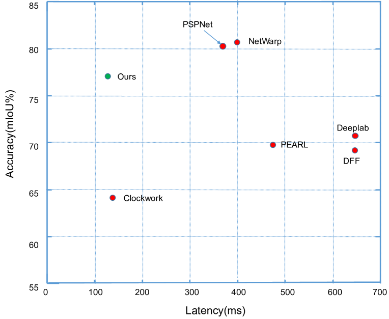
Previous efforts on video semantic segmentation mainly fall into two classes, namely high-level modeling and feature-level propagation. The former [8, 21] integrates frame-wise analysis via a sequential model. The methods along this line usually add additional levels on top, and therefore are unable to reduce the computing cost. The latter, such as Clockwork Net [25] and Deep Feature Flow [31], instead attempts to reuse the features in preceding frames to accelerate computation. Such methods were designed to reduce the overall cost in an amortized sense, while neglecting the issue of latency. Moreover, from a technical standpoint, existing methods exploit temporal correlations by treating all locations independently and uniformly. It ignores the different characteristics between smooth regions and boundaries, and lacks the flexibility of handling complex variations. Fig. 1 compares the performance/latency tradeoffs of various methods. We can see that previous methods fall short in either aspect.

Our primary goal in this work is to reduce not only the overall cost but also the maximum latency, while maintaining competitive performance in complicated and ever-changing scenarios. Towards this goal, we explore a new framework. Here, we adopt the idea of feature sharing, but move beyond the limitations of previous methods in two important aspects. (1) We introduce an adaptive feature propagation component, which combines features from preceding frames via spatially variant convolution. By adapting the combination weights locally, it results in more effective use of previous features and thus higher segmentation accuracy. (2) We adaptively allocate the keyframes on demand based on accuracy prediction and incorporate a parallel scheme to coordinate keyframe computation and feature propagation. This way not only leads to more efficient use of computational resources but also reduce the maximum latency. These components are integrated into a network.

Overall, the contributions of this work lie in three key aspects. (1) We study the issue of latency, which is often overlooked in previous work, and present a framework that achieves low-latency video segmentation. (2) We introduce two new components: a network using spatially variant convolution to propagate features adaptively and an adaptive scheduler to reduce the overall computing cost and ensure low latency. (3) Experimental results on both Cityscapes and CamVid demonstrate that our method achieve competitive performance as compared to the state of the art with remarkably lower latency.

2 Related Work

Image Semantic Segmentation

Semantic segmentation predicts per-pixel semantic labels given the input image. The Fully Convolutional Network (FCN) [19] is a seminal work on this topic, which replaces fully-connected layers in a classification network by convolutions to achieve pixel-wise prediction. Extensions to this formulation mainly follow two directions. One is to apply Conditional Random Fields (CRF) or their variants on top of the CNN models to increase localization accuracy [4, 18, 30]. The other direction explores multi-scale architectures to combine both low-level and high-level features [5, 11]. Various improved designs were proposed in recent years. Noh et al. [22] proposed to learn a deconvolution network for segmentation. Badrinarayanan et al. [1] proposed SegNet, which adopts an encoder-decoder architecture and leverages max pooling indices for upsampling. Paszke et al. [23] focused on the efficiency and developed ENet, a highly efficient network for segmentation. Zhao et al. [29] presented the PSPNet, which uses pyramid spatial pooling to combine global and local cues. All these works are purely image-based. Even if applied to videos, they work on a per-frame basis without considering the temporal relations.

Video Semantic Segmentation

Existing video semantic segmentation methods roughly fall in two categories. One category is to improve the accuracy by exploiting temporal continuity. Fayyaz et al. [8] proposed a spatial-temporal LSTM on per-frame CNN features. Nilsson and Sminchisescu [21] proposed gated recurrent units to propagate semantic labels. Jin et al. [14] proposed to learn discriminative features by predicting future frames and combine both the predicted results and current features to parse a frame. Gadde et al. [10] proposed to combine the features wrapped from previous frames with flows and those from the current frame to predict the segmentation. While these methods improve the segmentation accuracy by exploting across-frame relations, they are built on per-frame feature computation and therefore are not able to reduce the computation.

Another category focuses instead on reducing the computing cost. Clockwork Net [25] adapts mutli-stages FCN and directly reuses the second or third stage features of preceding frames to save computation. Whereas the high level features are relatively stable, such simple replication is not the best practice in general, especially when signficant changes occur in the scene. The DFF [31] propagates the high level feature from the key frame to current frame by optical flow learned in a flow network [9] and obtains better performance. Nevertheless, the separate flow network increases the computational cost; while the per-pixel location transformation by optical flow may miss the spatial information in the feature field. For both methods, the key frame selection is crucial to the overall performance. However, they simply use fixed-interval schedules [25, 31] or heuristic thresholding schemes [25], without providing a detailed investigation. Moreover, while being able to reduce the overall cost, they do not decrease the maximum latency.

There are also other video segmentation methods but with different settings. Perazzi et al. [24] built a large scale video object segmentation dataset, which concerns about segmenting the foreground objects and thus are different from our task, parsing the entire scene. Khoreva et al. [15] proposed to learn smooth video prediction from static images by combining the results from previous frames. Caelles et al. [3] tackled this problem in a semi-supervised manner. Mahasseni et al. [20] developed an offline method, which relies on a Markov decision process to select key frames, and propagate the results on key frames to others via interpolation. This method needs to traverse the video frames back and forth, and therefore is not suitable for the online settings discussed in this paper.

3 Video Segmentation Framework

We develop an efficient framework for video semantic segmentation. Our goal is to reduce not only the overall computing cost but also the maximum latency, while maintaining competitive performance. Specifically, we adopt the basic paradigm of the state-of-the-art frameworks [25, 31], namely, propagating features from key frames to others by exploiting the strong correlations between adjacent frames. But we take a significant step further, overcoming the limitations of previous work with new solutions to two key problems: (1) how to select the key frames and (2) how to propagate features across frames.

Figure 2: The overall pipeline. At each time step $t$, the lower-part of the CNN $S_{l}$ first computes the low-level features $F_{l}^{t}$. Based on both $F_{l}^{k}$ (the low-level features of the previous key frame) and $F_{l}^{t}$, the framework will decide whether to set $I^{t}$ as a new key frame. If yes, the high-level features $F_{h}^{t}$ will be computed based on the expensive higher-part $S_{h}$; otherwise, they will be derived by propagating from $F_{h}^{k}$ using spatially variant convolution. The high-level features, obtained in either way, will be used in predicting semantic labels.

3.1 Framework Overview

Previous works usually select key frames based on fixed intervals [31] or simple heuristics [25], and propagate features based on optical flows that are costly to compute [31] or CNNs with fixed kernels. Such methods often lack the capability of handling complex variations in videos, e.g. the changes in camera motion or scene structures. In this work, we explore a new idea to tackle these problems – taking advantage of low-level features, i.e. those from lower layers of a CNN. Specifically, low-level features are inexpensive to obtain, yet they provide rich information about the characteristics of the underlying frames. Hence, we may select key frames and propagate features more effectively by exploiting the information contained in the low-level features, while maintaining a relatively low computing cost.

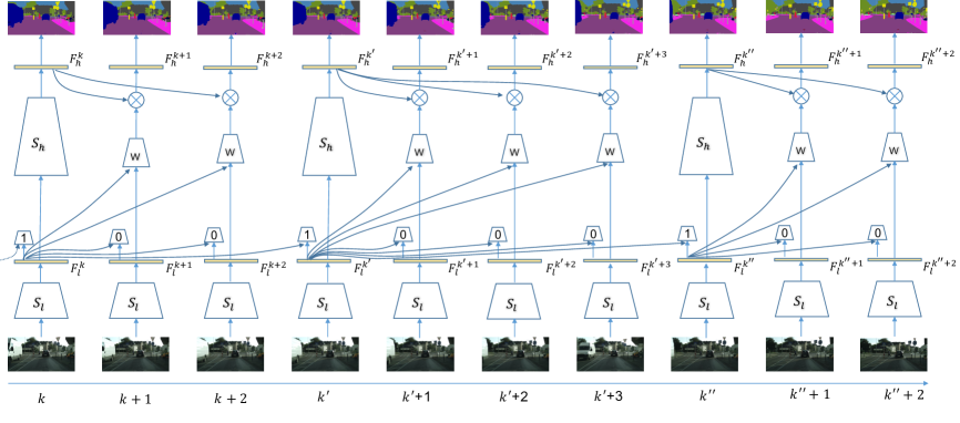
Figure 2 shows the overall pipeline of our framework. Specifically, we use a deep convolutional network (ResNet-101 [12] in our implementation) to extract visual features from frames. We divide the network into two parts, the lower part $S_{l}$ and the higher-part $S_{h}$. The low-level features derived from $S_{l}$ will be used for selecting key frames and controlling how high-level features are propagated.

At runtime, to initialize the entire procedure, the framework will feed the first frame $I^{0}$ through the entire CNN and obtain both low-level and high-level features. At a later time step $t$, it performs the computation adaptively. In particular, it first feeds the corresponding frame $I^{t}$ to $S_{l}$, and computes the low-level features $F_{l}^{t}$. Based on $F_{l}^{t}$, it decides whether to treat $I^{t}$ as a new key frame, depending on how much it deviates from the previous one. If the decision is “yes”, it will continue to feed $F_{l}^{t}$ to $S_{h}$ to compute the high-level features $F_{h}^{t}$, and then the segmentation map (via pixel-wise classification). Otherwise, it will feed $F_{l}^{t}$ to a kernel predictor, obtain a set of convolution kernels therefrom, and use them to propagate the high-level features from the previous key frame via spatially variant convolution.

Note that the combined cost of kernel prediction and spatially variant convolution is dramatically lower than computing the high-level features from $F_{l}^{t}$ ($38$ ms vs $299$ ms). With our design, such an adaptive propagation scheme can maintain reasonably high accuracy for a certain range ($7$ frames) from a key frame. Moreover, the process of deciding whether $I^{t}$ is a key frame is also cheap ($20$ ms). Hence, by selecting key frames smartly and propagating features effectively, we can significantly reduce the overall cost.

3.2 Adaptive Selection of Key Frames

An important step in our pipeline is to decide which frames are the key frames. A good strategy is to select key frames more frequently when the video is experiencing rapid changes, while reducing the computation when the observed scene is stable. Whereas this has been mentioned in previous literatures, what dominate the practice are still fixed-rate schedulers [31] or those based on simple thresholding of feature variances [25].

According to the rationale above, a natural criterion for judging whether a frame should be chosen as a new key frame is the deviation of its segmentation map from that of the previous key frame. This can be formally defined as the fraction of pixels at which the semantic labels differ. Intuitively, a large deviation implies significant changes and therefore it would be the time to set a new key frame.

However, computing the deviation as defined above requires the segmentation map of the current frame, which is expensive to obtain. Our approach to this problem is to leverage the low-level features to predict its value. Specifically, we conducted an empirical study on both Cityscapes and Camvid datasets, and found that there exists strong correlation between the difference in low-level features and the deviation values. Greater differences in the low-level features usually indicate larger deviations.

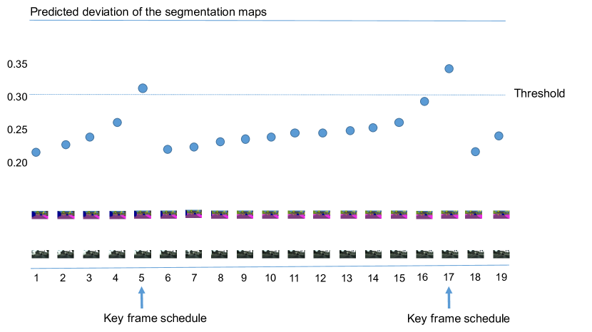
Motivated by this observation, we devise a small neural network to make the prediction. Let $k$ and $t$ be the indexes of two frames, this network takes the differences between their low-level features, i.e. $(F_{l}^{t}-F_{l}^{k})$, as input, and predicts the segmentation deviation, denoted by $\mathrm{dev}_{S}(k,t)$. Specifically, our design of this prediction network comprises two convolutional kernels with $256$ channels, a global pooling and a fully-connected layer that follows. In runtime, at time step $t$, we use this network to predict the deviation from the previous key frame, after the low-level features are extracted. As shown in Figure 3, we observed that the predicted deviation would generally increases over time. If the predicted deviation goes beyond a pre-defined threshold, we set the current frame as a key frame, and computes its high-level features with $S_{h}$, the higher part of the CNN.

Figure 3: Adaptive key frame selection. As we proceed further away from the key frame, the predicted deviation of the segmentation map, depicted with blue dots, gradually increases. In our scheme, when the deviation goes beyond a pre-defined threshold, the current frame will be selected as a new key frame.

3.3 Adaptive Feature Propagation

As mentioned, for a frame $I^{t}$ that is not a key frame, its high-level features will be derived by propagating from the previous key frame, which we denote by $I^{k}$. The question of how to propagate features effectively and efficiently is nontrivial. Existing works often adopt either of the following two approaches. 1) Follow optical flows [31]. While sounding reasonable, this way has two drawbacks: (a) The optical flows are expensive to compute. (b) Point-to-point mapping is often too restrictive. For high-level feature maps, where each feature actually captures the visual patterns over a neighborhood instead of a single site, a linear combination may provide greater latitude to express the propagation more accurately. 2) Use translation-invariant convolution [20]. While convolution is generally less expensive and offers greater flexibility, using a fixed set of convolution kernels uniformly across the map is problematic. Different parts of the scene have different motion patterns, e.g. they may move towards different directions, therefore they need different weights to propagate.

Motivated by this analysis, we propose to propagate the features by spatially variant convolution, that is, using convolution to express linear combinations of neighbors, with the kernels varying across sites. Let the size of the kernels be $H_{K}\times H_{K}$, then the propagation from the high-level features of the previous key frame ($F_{h}^{k}$) to that of the current frame ($F_{h}^{t}$) can be expressed as

$$F_{h}^{t}(l,i,j)=\sum_{u=-\Delta}^{\Delta}\sum_{v=-\Delta}^{\Delta}W^{(k,t)}_{ij}(u,v)\cdot F_{h}^{k}(l,i-u,j-v).$$ (1)

Here, $\Delta=\left\lfloor{H_{K}/2}\right\rfloor$, $F_{h}^{t}(l,i,j)$ is the feature value at $(i,j)$ of the $l$-th channel in $F_{h}^{t}$, $W^{(k,t)}_{ij}$ is an $H\times H$ kernel used to compute the feature at $(i,j)$ when propagating from $F_{h}^{k}$ to $F_{h}^{t}$. Note that the kernel values are to assign weights to different neighbors, which are dependent on the feature location $(i,j)$ but shared across all channels.

Figure 4: Adaptive feature propagation. Let $t$ refer to the current frame and $k$ the previous key frame. When the low-level features $F_{l}^{t}$ are computed, the kernel weight predictor will take both $F_{l}^{k}$ and $F_{l}^{t}$ as input, and yield a series of convolution kernels, each for a different location. Then the high-level features in the previous key frame $F_{h}^{k}$ will be propagated to the current time step via spatially variant convolution using the predicted kernels. Finally, the high-level features will be used in pixel-wise label prediction.

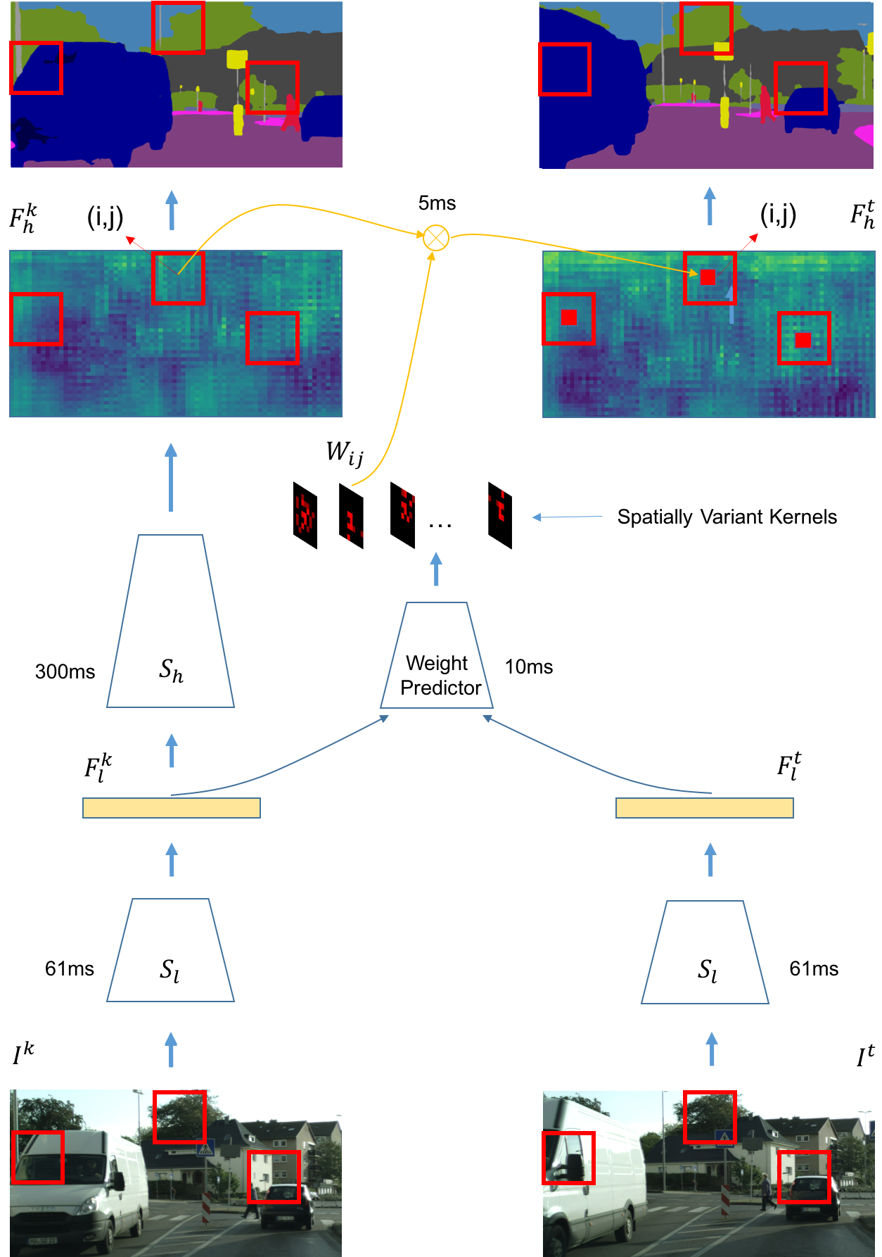
There remains a question – how to obtain the spatially variant kernels $W_{ij}^{(k,t)}$. Again, we leverage low-level features to solve the problem. In particular, we devise a kernel weight predictor, which is a small network that takes the low-level features of both frames, $F_{l}^{k}$ and $F_{l}^{t}$, as input, and produces the kernels at all locations altogether. This network comprises three convolutional layers interlaced with ReLU layers. The output of the last convolutional layer is of size $H_{K}^{2}\times H\times W$, where $H\times W$ is the spatial size of the high-level feature map. This means that it outputs an $H_{K}^{2}$-channel vector at each location, which is then repurposed to be a kernel of size $H_{K}\times H_{K}$ for that location. This output is then converted to normalized weights via a softmax layer to ensure that the weights of each kernel sum to one. With the weights decided on the low-level features, we allow the kernels to be adapted to not only the locations but also the frame contents, thus obtaining great expressive power.

To increase the robustness against scene changes, we fuse the low-level features $F_{l}^{t}$ with the propagated high-level feature $F_{h}^{t}$ for predicting the labels. Unlike in original Clockwork Net [25], where low- and high-level features are simply concatenated, we introduce a low-cost AdaptNet to adapt the low-level features before it is used for prediction. The AdaptNet consists of three convolution layers and each layer has a small number of channels. The AdaptNet is jointly learned with the weight predictor in model training. In this way, the framework can learn to exploit the complementary natures of both components more effectively.

3.4 Low-Latency Scheduling

Low latency is very important in many real-world applications, e.g. surveillance and autonomous driving. Yet, it has not received much attention in previous works. While some existing designs [25] can reduce the overall cost in an amortized sense, the maximum latency is not decreased in this design due to the heavy computation at key frames.

Based on the framework presented above, we devise a new scheduling scheme that can substantially reduce the maximum latency. The key of our approach is to introduce a “fast track” at key frames. Specifically, when a frame $I^{t}$ is decided to be a key frame, this scheme will compute the segmentation of this frame through the “fast track”, i.e. via feature propagation. The high-level features resulted from the fast track are temporarily treated as the new key frame feature and placed in the cache. In the mean time, a background process is launched to compute the more accurate version of $F_{h}^{t}$ via the “slow track” $S_{h}$, without blocking the main procedure. When the computation is done, this version will replace the cached features.

Our experiments show that this design can significantly reduce the maximum latency (from $360$ ms to $119$ ms), only causing minor drop in accuracy (from $76.84\%$ to $75.89\%$). Hence, it is a very effective scheme for real-world applications, especially those with stringent latency constraints. Note that the low-latency scheme cannot work in isolation. This good balance between performance and latency can only be achieved when the low-latency scheme is working with the adaptive key-frame selection and the adaptive feature propagation modules presented above.

4 Implementation Details

Our basic network is a ResNet-101 [12] pretrained on ImageNet. We choose conv4_3 as the split point between the lower and higher parts of the network. The low-level features $F_{l}^{t}$ derived from this layer has $1024$ channels. The lower part consumes about $1/6$ of the total inference time. In general, the model can achieve higher accuracy with a heavier low-level part, but at the expense of higher computing cost. We chose conv4_3 as it attains a good tradeoff between accuracy and speed on the validation sets.

The adaptive key frame selector takes the low-level features of the current frame $F_{l}^{t}$ and that of the previous key frame $F_{l}^{k}$ as input. This module first reduces the input features to $256$ channels with a convolution layer with $3\times 3$ kernels and then compute their differences, which are subsequently fed to another convolution layer with $256$ channels and $3\times 3$ kernels. Finally, a global pooling and a fully-connected layer are used to predict the deviation.

The kernel weight predictor in the adaptive feature propagation module (see Fig. 4) has a similar structure, except that the input features are concatenated after being reduced to $256$ channels, the global pooling is removed, and the fully-connected layer is replaced by a convolution layer with $1\times 1$ kernels and $81$ channels. The AdaptNet also reduces the low-level features to $256$ channels by a convolution layer with $3\times 3$ kernels, and then pass them to two two convolution layers with $256$ channels and $3\times 3$ kernels. For non-key frames, the adapted low-level features, i.e. the output of the AdaptNet are fused with the propagated high-level features. The fusion process takes the concatenation of both features as input, and sends it through a convolution layer with $3\times 3$ kernels and $256$ channels.

During training, we first trained basic network with respective ground-truths and fixed it as the feature extractor. Then, we finetuned the adaptive propagation module and the adaptive schedule module, both of which can take a pair of frames that are $l$ steps apart as input ($l$ is randomly chosen in $[2,10]$). Here, we choose the pairs such that in each pair the first frame is treated as the key frame, and the second one comes with annotation. For the adaptive propagation module, the kernel predictor and the AdaptNet are integrated into a network. This integrated network can produce a segmentation map for the second frame in each pair through keyframe computation and propagation. This combined network is trained to minimize the loss between the predicted segmentation (on the second frame of each pair) and the annotated groundtruth. For training the adaptive schedule module, we generated the segmentation maps of all unlabelled frames as auxiliary labels based on the trained basic network and computed the deviation of the segmentation maps between key frame and current frame as the regression target. The training images were randomly cropped to $713\times 713$ pixels. No other data argumentation methods were used.

5 Experiment

We evaluated our framework on two challenging datasets, Cityscapes [7] and CamVid [2], and compared it with state-of-the-art approaches. Our method, with lowest latency, outperforms previous methods significantly.

5.1 Datasets and Evaluation Metrics

Cityscapes [7] is set up for urban scene understanding and autonomous driving. It contains snippets of street scenes collected from $50$ different cities, at a frame rate of $17$ fps. The training, validation, and test sets respectively contain $2975$, $500$, and $1525$ snippets. Each snippet has $30$ frames, where the $20$-th frame is annotated with pixel-level ground-truth labels for semantic segmentation with $19$ categories. The segmentation accuracy is measured by the pixel-level mean Intersection-over-Union (mIoU) scores.

Camvid [2] contains $701$ color images with annotations of $11$ semantic classes. These images are extracted from driving videos captured at daytime and dusk. Each video contains $5000$ frames on average, with a resolution of $720\times 960$ pixels. Totally, there are about $40K$ frames.

5.2 Evaluation on Cityscapes Dataset

Method	mIOU	Avg RT	Latency
Clockwork Net [25]	67.7%	141ms	360ms
Deep Fea. Flow [31]	70.1%	273ms	654ms
GRFP(5) [21]	69.4%	470ms	470ms
baseline	80.2%	360ms	360ms
AFP + fix schedule	75.26%	151ms	360ms
AFP + AKS	76.84%	171ms	380ms
AFP + AKS + LLS	75.89%	119ms	119ms

Table 1: Comparison with state-of-the-art on Cityscapes dataset. “Avg RT” means average runtime per frame. “AFP” means adaptive feature propopagation. “fix schedule” means key frame is selected very 5 frame. “AKS” means adaptive key frame selection. “LLS” means low-latency scheduling scheme. Clockwork Net is implmented with the same settings as our method with fix schedule: (a) the same backbone network (ResNet-101), (b) the same split between the low-level and high-level stages, (c) the same AdaptNet following the low-level stage, and (d) the same interval between keyframes ($l=5$).

We compared our low-latency video semantic segmentation framework with recent state-of-the-art methods, following their evaluation protocol. Table 1 shows the quantitative comparison. The baseline is per-frame segmentation with the full ResNet. Our adaptive feature propagation with fixed-interval schedule speeds up the pipeline, reducing the per-frame runtime from $360$ ms to $151$ ms while decreasing the performance by $4.9\%$. Using adaptive key frame selection, the performance is boosted by $1.6\%$. While these schemes reduce the overall runtime, they are not able to reduce the maximum latency, due to the heavy computation on key frames. The low-latency scheduler effectively tackles this issue, which substantially decreases the latency to $119$ ms (about $1/3$ of the baseline latency) while maintaining a comparable performance (with just a minor drop).

From the results, we also see that other methods proposed recently fall short in certain aspects. In particular, Clockwork Net [25] has the same latency, but at the cost of significantly dropped performance. DFF [31] maintains a better performance, but at the expense of considerably increased computing cost and dramatically larger latency. Our final result, with low latency schedule for video segmentation, outperforms previous methods by a large margin. This validates the effectiveness of our entire design.

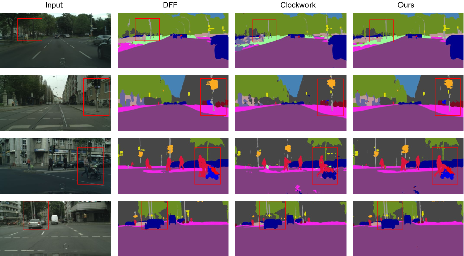
In addition to the quantitative comparison, we also shows some visual results in Fig. 6. Our method can successfully learn the video segmentation even when the frames vary significantly. In what follows, we will investigate the design for each module respectively.

Method	mIOU
Clockwork Propagation [25]	56.53%
Optical Flow Propagation [31]	69.2%
Unified Propagation	58.73%
Weight By Image Difference	60.12%
Adaptive Propagation Module (no fuse)	68.41%
Adaptive Propagation Module (with fuse)	75.26%

Table 2: Comparison of different feature propagation modules.

Figure 5: Comparison of different scheduling schemes.

Comparison on Feature Propagation

We begin by evaluating the effectiveness of our proposed adaptive propagation module. To evaluate the specific performance gain on this module, we fix the scheduling scheme as previous methods, namely selecting a key-frame per $5$ frames.

Table 2 shows the quantitative comparison. We compared our method with a globally learned unified propagation, for which the result is not satisfactory. It reveals that the spatially variant weight is quite important in our solution. We also compared to a baseline, where the weights are directly set by the differences of the input pixel values, our learned propagation weights also perform better. Our experiment also shows that the fuse with the low-level features from the current frame by AdaptNet achieves significant performance improvements (from $68.41\%$ to $75.26\%$), which may be ascribed to the strong complementary information learned by the fuse model.

Compared to recently proposed methods for feature propagation, our adaptive propagation module still performs significantly better. Particularly, Clockwork directly replaces parts of the current features with previous ones, and therefore the derived representation is not adapted to current changes, thus resulting in poor performance. The optical flow based method DFF [31] relies on the optical flows to propagate features and shows substantially better accuracies as compared to Clockwork, due to its better adaptivity. Yet, its performance is sensitive to the quality of the Flownet, and it ignores the spatial relationship on the feature space. These factors limit its performance gain, and hence it is still inferior to the proposed method.

Comparison on Scheduling

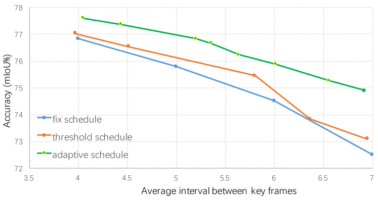
We also studied the performance of the adaptive scheduling module for key frame selection, given our feature propagation module. Note that a good schedule not only reduces the frequency of key frames, but also increases the performance given a fixed number of key frames. Hence, we conducted several experiments to compare different schedule methods across different key-frame intervals.

Specifically, we compared fixed rate schedule, threshold schedule, and also our adaptive schedule module. Fig. 5 shows the results. Under each key-frame interval, our adaptive schedule always outperforms the other two. We believe the reason why the proposed method outperforms the threshold schedule is that the intermediate feature maps is not specially optimized for key-frame selection. They may contain noises and perhaps many other irrelevant factors.

Modules	Time (ms)	R
Lower part of network $S_{l}$	61	16.9%
Higher part of network $S_{h}$	299	83.1%
Basic Network	360	100%
Adaptive Schedule Module	20	5.5%
Adaptive Propagation Module	38	10.5%
Non-Key Frame	119	33%

Table 3: Latency analysis for each module of our network. The second column (R) shows the ratio of the latency to the time spent by the basic network.

Cost and Latency Analysis

We analyzed the computation cost of each component in our pipeline, and then the overall latency of our method. The results are in Table 3. With the low-latency scheduling scheme, the total latency of our pipeline is equal to the sum of the lower part of the network $S_{l}$, adaptive key-frame selection, adaptive feature propagation, which is $0.119s$ ($33\%$ of the basic network). On the contrary, all previous methods fail to reduce latency in their system design, despite that they may reduce the overall cost in the amortized sense. Hence, they are not able to meet the latency requirements in real-time applications.

Methods	Pixel Accuracy	CA
SuperParsing [28]	83.9%	62.5%
DAG-RNN [26]	91.6%	78.1%
MPF-RNN [13]	92.8%	82.3%
RTDF [17]	89.9%	80.5%
PEARL [14]	94.2%	82.5%
Ours	94.6%	82.9%

Table 4: Result comparison for CamVid dataset.

Figure 6: Visual Results for Cityscapes Dataset: our method can achieve significant improvement shown as the red rectangle.

Figure 7: Visual Results for Camvid Dataset: our method can achieve significant improvement shown as the red rectangle.

5.3 CamVid Dataset

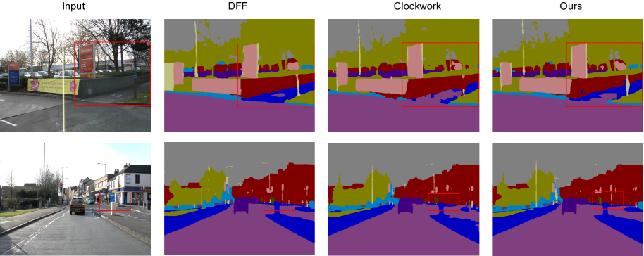
We also evaluated our method on CamVid, another video segmentation dataset, and compard it with multiple previous methods that have reported performances on CamVid, which range from traditional methods to various CNN or RNN based methods. In Table 4, we report the pixel accuracy and average per-Class Accuracy(CA), which can reduce the dominated effect on majority classes. We can see our framework still performs the best. The consistently good performances on both datasets show that our adaptive framework for video segmentation method is in general beneficial to video perception. Qualitative results on this dataset are shown in Fig. 7.

6 Conclusion

We presented an efficient video semantic segmentation framework with two key components: adaptive feature propagation and adaptive key-frame schedule. Particularly, our specially designed schedule scheme can achieve low latency in an online setting. The results on both Cityscapes and CamVid showed that our method can yield a substantially better tradeoff between accuracy in latency, compared to previous methods. In future, we will explore more model compression approaches which can further reduce the overall computation cost and latency for a practical system.

References

- [1] V. Badrinarayanan, A. Kendall, and R. Cipolla. Segnet: A deep convolutional encoder-decoder architecture for image segmentation. CoRR, abs/1511.00561, 2015.
- [2] G. J. Brostow, J. Fauqueur, and R. Cipolla. Semantic object classes in video: A high-definition ground truth database. Pattern Recognition Letters, 30(2):88–97, 2009.
- [3] S. Caelles, K.-K. Maninis, J. Pont-Tuset, L. Leal-Taixé, D. Cremers, and L. Van Gool. One-shot video object segmentation. arXiv preprint arXiv:1611.05198, 2016.
- [4] L. Chen, G. Papandreou, I. Kokkinos, K. Murphy, and A. L. Yuille. Semantic image segmentation with deep convolutional nets and fully connected crfs. CoRR, abs/1412.7062, 2014.
- [5] L. Chen, Y. Yang, J. Wang, W. Xu, and A. L. Yuille. Attention to scale: Scale-aware semantic image segmentation. CoRR, abs/1511.03339, 2015.
- [6] L.-C. Chen, G. Papandreou, I. Kokkinos, K. Murphy, and A. L. Yuille. Deeplab: Semantic image segmentation with deep convolutional nets, atrous convolution, and fully connected crfs. arXiv preprint arXiv:1606.00915, 2016.
- [7] M. Cordts, M. Omran, S. Ramos, T. Rehfeld, M. Enzweiler, R. Benenson, U. Franke, S. Roth, and B. Schiele. The cityscapes dataset for semantic urban scene understanding. In Proceedings of the IEEE Conference on Computer Vision and Pattern Recognition, pages 3213–3223, 2016.
- [8] M. Fayyaz, M. H. Saffar, M. Sabokrou, M. Fathy, R. Klette, and F. Huang. Stfcn: Spatio-temporal fcn for semantic video segmentation. arXiv preprint arXiv:1608.05971, 2016.
- [9] P. Fischer, A. Dosovitskiy, E. Ilg, P. Häusser, C. Hazırbaş, V. Golkov, P. van der Smagt, D. Cremers, and T. Brox. Flownet: Learning optical flow with convolutional networks. arXiv preprint arXiv:1504.06852, 2015.
- [10] R. Gadde, V. Jampani, and P. V. Gehler. Semantic video cnns through representation warping. arXiv preprint arXiv:1708.03088, 2017.
- [11] B. Hariharan, P. A. Arbeláez, R. B. Girshick, and J. Malik. Hypercolumns for object segmentation and fine-grained localization. In CVPR, pages 447–456, 2015.
- [12] K. He, X. Zhang, S. Ren, and J. Sun. Deep residual learning for image recognition. CoRR, abs/1512.03385, 2015.
- [13] X. Jin, Y. Chen, J. Feng, Z. Jie, and S. Yan. Multi-path feedback recurrent neural network for scene parsing. arXiv preprint arXiv:1608.07706, 2016.
- [14] X. Jin, X. Li, H. Xiao, X. Shen, Z. Lin, J. Yang, Y. Chen, J. Dong, L. Liu, Z. Jie, et al. Video scene parsing with predictive feature learning. arXiv preprint arXiv:1612.00119, 2016.
- [15] A. Khoreva, F. Perazzi, R. Benenson, B. Schiele, and A. Sorkine-Hornung. Learning video object segmentation from static images. arXiv preprint arXiv:1612.02646, 2016.
- [16] A. Krizhevsky, I. Sutskever, and G. E. Hinton. Imagenet classification with deep convolutional neural networks. In Advances in neural information processing systems, pages 1097–1105, 2012.
- [17] P. Lei and S. Todorovic. Recurrent temporal deep field for semantic video labeling. In European Conference on Computer Vision, pages 302–317. Springer, 2016.
- [18] Z. Liu, X. Li, P. Luo, C. C. Loy, and X. Tang. Semantic image segmentation via deep parsing network. In ICCV, pages 1377–1385, 2015.
- [19] J. Long, E. Shelhamer, and T. Darrell. Fully convolutional networks for semantic segmentation. In CVPR, pages 3431–3440, 2015.
- [20] B. Mahasseni, S. Todorovic, and A. Fern. Budget-aware deep semantic video segmentation. In Proceedings of the IEEE Conference on Computer Vision and Pattern Recognition, pages 1029–1038, 2017.
- [21] D. Nilsson and C. Sminchisescu. Semantic video segmentation by gated recurrent flow propagation. arXiv preprint arXiv:1612.08871, 2016.
- [22] H. Noh, S. Hong, and B. Han. Learning deconvolution network for semantic segmentation. In ICCV, pages 1520–1528, 2015.
- [23] A. Paszke, A. Chaurasia, S. Kim, and E. Culurciello. Enet: A deep neural network architecture for real-time semantic segmentation. CoRR, abs/1606.02147, 2016.
- [24] F. Perazzi, J. Pont-Tuset, B. McWilliams, L. Van Gool, M. Gross, and A. Sorkine-Hornung. A benchmark dataset and evaluation methodology for video object segmentation. In Proceedings of the IEEE Conference on Computer Vision and Pattern Recognition, pages 724–732, 2016.
- [25] E. Shelhamer, K. Rakelly, J. Hoffman, and T. Darrell. Clockwork convnets for video semantic segmentation. In Computer Vision–ECCV 2016 Workshops, pages 852–868. Springer, 2016.
- [26] B. Shuai, Z. Zuo, B. Wang, and G. Wang. Dag-recurrent neural networks for scene labeling. In Proceedings of the IEEE Conference on Computer Vision and Pattern Recognition, pages 3620–3629, 2016.
- [27] K. Simonyan and A. Zisserman. Very deep convolutional networks for large-scale image recognition. CoRR, abs/1409.1556, 2014.
- [28] J. Tighe and S. Lazebnik. Superparsing: scalable nonparametric image parsing with superpixels. In European conference on computer vision, pages 352–365. Springer, 2010.
- [29] H. Zhao, J. Shi, X. Qi, X. Wang, and J. Jia. Pyramid scene parsing network. arXiv preprint arXiv:1612.01105, 2016.
- [30] S. Zheng, S. Jayasumana, B. Romera-Paredes, V. Vineet, Z. Su, D. Du, C. Huang, and P. H. S. Torr. Conditional random fields as recurrent neural networks. In ICCV, pages 1529–1537, 2015.
- [31] X. Zhu, Y. Xiong, J. Dai, L. Yuan, and Y. Wei. Deep feature flow for video recognition. In Proceedings of the IEEE Conference on Computer Vision and Pattern Recognition, pages 2349–2358, 2017.