Linked cluster expansion of the many-body path integral

Abstract

We develop an approach of calculating the many-body path integral based on the linked cluster expansion method. First, we derive a linked cluster expansion and we give the diagrammatic rules for calculating the free-energy and the pair distribution function $g(r)$ as a systematic power series expansion in the particle density. We also generalize the hypernetted-chain (HNC) equation for $g(r)$, known from its application to classical statistical mechanics, to a set of quantum HNC equations (QHNC) for the quantum case. The calculated $g(r)$ for distinguishable particles interacting with a Lennard-Jones potential in various attempted schemes of approximation of the diagrammatic series compares very well with the results of path integral Monte Carlo simulation even for densities as high as the equilibrium density of the strongly correlated liquid ⁴He. Our method is applicable to a wide range of problems of current general interest and may be extended to the case of identical particles and, in particular, to the case of the many-fermion problem.

I Introduction

With the advance of computational power during the last four decades, Monte Carlo simulations have been very successful in addressing a volume of issues of classical statistical mechanics. As a result, earlier methods based on other approximate computational techniques, such as the cluster expansionMayer and Mayer (1940)Goodstein (2002) in conjunction with the hypernetted-chain approach (HNC)Hiroike (1957a, b); Morita (1958, 1959); Morita and Hiroike (1961); Morita (1960); Morita and Hiroike (1960) have become much less popular and are rather rarely used. Furthermore, the Monte Carlo method has been extended to carry out simulations of quantum many-body systems. It has been successfully developed to treat accurately a variety of problems including, quantum-spin systems, the polaron problemProkof’ev and Svistunov (1998); Mishchenko et al. (2000), and bosonic systems in the regime of high particle-density and as strongly correlated as liquid ⁴HeCeperley (1995). There are problems, however, such as the many-fermion systems and frustrated quantum spin systems, where there is no useful a priori positive-definite quantity to be used as the sampling probability in the Markov process. There are many useful ideas on how to treat these problems within some approximation scheme, such as, the fixed node approximationMcMahon et al. (2012) or the constrained path Monte CarloZhang et al. (1997), however, they are limited in the regime of their applicability.

In the present paper we develop a cluster expansion technique to treat the quantum many-body Feynman path-integralFeynman and Hibbs (1965) at finite-temperatureFeynman (1998). The expansion can be regarded as a systematic expansion in the number of particles involved in the diagrams retained, i.e., keeping up to $n$-body clusters. Alternatively, this can be viewed as a systematic formal expansion in the particle density $\rho$. We tested the method by comparing our results for the pair distribution function $g(r)$ for distinguishable particles interacting with the Lennard-Jones interaction to the results obtained by the path integral Monte Carlo (PIMC) method. Our results for $g(r)$ in a wide distance-range obtained by keeping just up to three-body clusters are in good agreement with the results of the PIMC method even at ⁴He densities down to moderately low temperature. Furthermore, we generalize the HNC resummation approach to the quantum case (QHNC). We show that our results for distinguishable particles described by the Lennard-Jones interaction are in good agreement with the results obtained by the PIMC method for the same system. In particular, we are encouraged by the fact that the results for $g(r)$ are accurate for the high-density regime applicable to helium where short-range correlations are strong.

This method is generalizable to the case of identical particles and, therefore, it has the potential to be useful as an alternative approach to the treatment of fermionic systems or frustrated quantum-spin systems. While the approach of keeping up to $n$-body clusters and the QHNC approach are both approximations, they may provide alternative approaches to complex problems from a different angle. For example, while at high density the electron gasCeperley and Alder (1980) is accurately described by the random phase approximation Fetter and Walecka (2003); Bohm and Pines (1953), at low-density, there is no exact treatment. Our method, which becomes asymptotically exact in the low-density limit, could provide the still missing accurate approach for the electron gas at low densities. Furthermore, the approach developed in the present work is a general method to treat the quantum many-particle problem. Therefore, it can be applied to other systems in diverse areas of physics, such as, systems of trapped ultra-cold atoms, and possibly to the many-nucleon problemPandharipande and Wiringa (1979), i.e., the hypothetical infinite nuclear matter and neutron stars.

The paper is organized as follows. In Sec. II we discuss the many-body path integral and we cast it in a form useful for the application of our method. In Sec. III we develop the cluster expansion of the path integral that describes the quantum mechanical partition function for a system of distinguishable particles. We give the diagrammatic rules for a systematic inclusion of all the diagrams order by order in the density. In Sec. IV we discuss the cluster expansion of the free-energy and in Sec. V that of the pair distribution function. In Sec. VI we present out results of the method viewed as a systematic power series expansion in the density. In addition, we derive the quantum hypernetted-chain (QHNC) equations and we give our results for the Lennard-Jones system for densities near the equilibrium density of liquid ⁴He. Last, in Sec. VII we present our conclusions.

II The many-body path integral

To build the path integral cluster expansion formalism we will follow the same procedure that is used in the case of classical cluster expansion. While our goal in this paper is to study the simpler case of distinguishable particles, we first begin by writing down the partition function Feynman (1998) for a system of $N$ interacting identical particles:

$$Z = \frac{1}{N!}\underset{P}{\sum}(\pm 1)^{[P]}\int d^{3}\vec{r}_{1}d^{3}\vec{r}_{2}....d^{3}\vec{r}_{N}$$ (1)

$$\langle\vec{r}_{1},\vec{r}_{2},...,\vec{r}_{N}\mid e^{-\beta\hat{H}}\mid\vec{r}_{P1},\vec{r}_{P2},...,\vec{r}_{PN}\rangle.$$

Here, the summation over $P$ means a summation over all permutations of particles and the notation $[P]$ denotes the order of the permutationFeynman (1998). In the case of bosons all permutations contribute with a positive sign. In the case of fermions, $(-1)^{[P]}$ is +1 or -1 depending on whether the permutation is even or odd. In the positions $(\vec{r}_{P1},\vec{r}_{P2},...,\vec{r}_{PN})$ the indices $P1,P2,...,PN$ are the particle indices after permutation $P$. In this paper we will deal with the general case of an interacting Hamiltonian $\hat{H}$ of the following form:

$$\hat{H}=-\frac{\hbar^{2}}{2m}\overset{N}{\underset{i}{\sum}}\nabla_{i}^{2}+\underset{i<j}{\sum}v(r_{ij}).$$ (2)

Next, we divide the imaginary-time interval $[0,\theta]$ ($\theta\equiv\hbar\beta$) into $M$ slices of size $\delta\tau=\hbar\beta/M$ to write $e^{-\beta\hat{H}}=e^{-\delta\tau\hat{H}/\hbar}e^{-\delta\tau\hat{H}/\hbar}...e^{-\delta\tau\hat{H}/\hbar}$. As usual we insert in between each pair of these operators the unit operator expressed as a sum over the complete set of many-body position eigenstates and by using the Trotter approximation we can write the partition function as:

$$Z = \underset{P}{\sum}\frac{(\pm 1)^{[P]}}{N!}\int_{\vec{r}_{i}(\theta)=\vec{r}_{Pi}(0)}\prod_{n=1}^{N}\prod_{k=0}^{M-1}\frac{d^{3}\vec{r}_{n}^{(k)}}{\lambda^{3}_{\delta\tau}}e^{-S_{E}},$$ (3)

where,

$$S_{E} = \frac{\delta\tau}{\hbar}\overset{M-1}{\underset{k=0}{\sum}}\underset{i<j}{\sum}\Bigl{[}\frac{m}{2{(\delta\tau)}^{2}}r^{2}_{i}(kk+1)+v(r_{ij}^{(k)})\Bigr{]},$$ (4)

$$\lambda_{\tau} \equiv {(2\pi\hbar\tau/m)^{1/2}},$$ (5)

and $r^{(k)}_{ij}=|\vec{r}^{(k)}_{i}-\vec{r}^{(k)}_{j}|$ and $r_{i}(kl)=|\vec{r}_{i}^{(k)}-\vec{r}_{i}^{(l)}|$. The constraint ${\vec{r}_{i}(\theta)=\vec{r}_{Pi}(0)}$ on the path integral (where $\theta=\hbar\beta$) means that the sum is over all possible $N$-particle paths which start at positions $(\vec{r}_{1}(0),\vec{r}_{2}(0),...,\vec{r}_{N}(0))$ at imaginary-time $\tau=0$ and after the “lapse” of an imaginary-time interval of $\beta\hbar$ they end up at positions $(\vec{r}_{1}(\theta)=\vec{r}_{P1}(0),\vec{r}_{2}(\theta)=\vec{r}_{P2}(0),...,\vec{r}_{N}(\theta)=\vec{r}_{PN}(0))$ where $P1,P2,...,PN$ are the particle indices after permutation $P$.

By taking the limit $M\rightarrow\infty$, one can obtain the well-known Feynman’s path-integral expression:

$$Z=\frac{1}{N!}\underset{P}{\sum}(-1)^{[P]}\int_{\vec{r}_{i}(\theta)=\vec{r}_{Pi}(0)}{\cal D}\vec{r}_{1}{\cal D}\vec{r}_{2}...{\cal D}\vec{r}_{N}e^{-S_{E}},$$ (6)

The Euclidean action in the above path integral is given by

$$S_{E}=\int_{0}^{\hbar\beta}(\sum_{i=1}^{N}\frac{1}{2}m\dot{\vec{r}}_{i}^{2}+\sum_{i<j}v(r_{ij}(\tau)))d\tau,$$ (7)

where $r_{ij}(\tau)=|\vec{r_{i}}(\tau)-\vec{r}_{j}(\tau)|$.

However, the Feynman’s path-integral expression is only symbolic and, for all practical purposes, we make use of the expression given by Eq. 3. As discussed in the abstract and in the introduction of this paper, in this paper we concentrate our attention to the simpler case of distinguishable particles, which corresponds to considering the identity permutation only.

III Cluster expansion of partition function

In this paper we concentrate only on the identity permutation which corresponds to a system of interacting distinguishable particles. This will allow us to test the method by comparison of our results to PIMC which is accurate in this case because of the absence of the sign problem. Since our method is diagrammatic in nature, it can be extended to include diagrams which correspond to particle permutations. Therefore, if we can demonstrate that the method works for distinguishable particles, it would be a promising sign for the applicability of the method to the more-complex problem of identical particles and in particular the problem of Fermions where QMC fails to address it in an exact way. While we consider the case of distinguishable particles, as we describe our method in the present paper, when appropriate, we address the generalizations needed in order to include the permutations.

Now, we concentrate on the dimensionless ratio $Z\over Z_{0}$ where $Z_{0}$ is the non-interacting partition function, which can be obtained from Eq. 3 by using the free-action, obtained from Eq. 4 with $v(r^{(k)}_{ij})=0$, and carrying out the Gaussian integrals:

$$Z_{0}=\frac{1}{N!}\Bigl{(}\frac{V}{V_{\theta}}\Bigr{)}^{N},\hskip 14.45377ptV_{\theta}=\lambda^{3}_{\theta},$$ (8)

and since $\lambda_{\theta}$ is the de Broglie thermal wavelength, $V_{\theta}$ is the de Broglie thermal volume. Thus,

$$\frac{Z}{Z_{0}}=\Bigl{(}\frac{V_{\theta}}{V}\Bigr{)}^{N}Z.$$ (9)

Next, we start the cluster expansion by defining the function $h_{ij}^{(k)}$ as follows:

$$e^{-\frac{\delta\tau}{\hbar}v(r_{ij}^{(k)})} \equiv 1+h_{ij}^{(k)},$$ (10)

and the function $L_{i}(kl)$ as follows:

$$L_{i}(kl) = \frac{1}{\lambda^{3}_{\tau_{kl}}}e^{-\pi\frac{r^{2}_{i}(kl)}{\lambda^{2}_{\tau_{kl}}}},$$ (11)

$$\tau_{kl} = |k-l|\delta\tau.$$ (12)

Using these definitions the partition function can be written as

$${Z\over{Z_{0}}} = \Bigl{(}\frac{V_{\theta}}{V}\Bigr{)}^{N}\int\prod_{n=1}^{N}\prod_{k=0}^{M-1}d^{3}r_{n}^{(k)}L_{n}(kk+1)$$ (13)

$$\times \prod_{l=0}^{M-1}\prod_{i<j}(1+h_{ij}^{(l)}).$$

The expression in Eq. 13 consists of products of $(1+h_{ij}^{(l))})$, which can be written out as follows:

$$\prod_{l=0}^{M-1}\prod_{i<j}(1+h_{ij}^{(l)})=1+\sum_{l=0}^{M-1}\sum_{i<j}h_{ij}^{(l)}+...$$ (14)

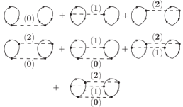
where we have omitted terms containing two or more $h$ factors. After substituting the expanded product in Eq. 9 we obtain a sum of integrals. We can keep track of terms by representing each of these integral terms by diagrams. As an example consider the case of 3 ($N=3$) particles with 3 time instants ($M=3$). In this case, the first few terms have been diagrammatically represented in Fig. 1.

Figure 1: Few diagrams that appear in the expression for $Z$ when $N=3$ and $M=3$.

We use the following convention for representing such terms:

1. The positions of the particles at the instants of time which enter in the integral are denoted by solid circles. An integration over these positions is implied.

2. $h_{ij}^{(k)}$ is denoted by a dashed line labeled by the index $(k)$ (which represents interaction between particles at the same instant of time $k$) connecting points $i$ and $j$.

3. The $L$ function defined by Eq. 11 is denoted by a solid line connecting points $\vec{r}_{i}^{(k)}$ and $\vec{r}_{i}^{(l)}$.

4. Every particle is associated with its own world-line, which is made up of products of $L$ functions. The world-lines of a pair of particles at a given instant of time can be either disconnected (i.e., there is a factor of unity) or they can be connected by a dashed-line.

5. The world-line starts at $\vec{r}_{1}^{(0)}$ and connects back to $\vec{r}_{1}^{(0)}$ because of the boundary condition $\vec{r}_{i}^{(0)}=\vec{r}_{i}^{(M)}$. Therefore, a world-line forms a loop formed by the particle positions at all instants of time.

In the case of identical particles, there are diagrams in which $\vec{r}_{i}^{(M)}=\vec{r}_{Pi}^{(0)}$, i.e., the particle positions are exchanged at imaginary-time slice $M$. In the present paper, we do not deal with the contribution of such diagrams.

If the world-line of a given particle has solid points which are not connected to any other point through dashed-lines then it is possible to perform the integration over those variables exactly by using the following identity:

$$L_{i}(kl)=\int d^{3}\vec{r}_{i}^{(m)}L_{i}(km)L_{i}(ml).$$ (15)

This result can be interpreted such that the world-line now makes a straight connection of the particle coordinate at the initial instant of time, i.e., $\vec{r}_{i}^{(k)}$ with the particle coordinate at the instant of time $\l$. This explicit integration removes such intermediate points in our diagrams which are not connected by any dashed-line. As an example, consider the diagram in Fig. 1. Because of the absence of dashed-lines it is possible to perform the integration over all three variables and the diagram equals to unity; Similarly, the term in Fig. 1 is obtained when the product is such that we have only one dashed-line (in this case $h_{12}^{(1)}$); here, particle 1 and 2 are connected but particle 3 is disconnected. Such a term has the following integral form:

$$\Bigl{(}{{V_{\theta}}\over V}\Bigr{)}^{3}\int\underset{i=1}{\overset{3}{\prod}}\underset{k=0}{\overset{2}{\prod}}d^{3}\vec{r}_{i}^{(k)}L_{i}(kk+1)h_{12}^{(2)}.$$ (16)

The coordinates of particle 3 at all instants of time can be integrated out and, thus, the diagram corresponds to the following expression:

$$\Bigl{(}{{V_{\theta}}\over V}\Bigr{)}^{2}\int\underset{i=1}{\overset{2}{\prod}}\underset{k=0}{\overset{2}{\prod}}d^{3}\vec{r}_{i}^{(k)}L_{i}(kk+1)h_{12}^{(2)}.$$ (17)

We can further simplify the above expression by noting that the integration over $\vec{r}_{1}^{(0)}$, $\vec{r}_{2}^{(0)}$, $\vec{r}_{1}^{(1)}$, and $\vec{r}_{2}^{(1)}$ can be performed as these are not connected through a dashed-line. The simplification leads to the following term:

$$\Bigl{(}{{V_{\theta}}\over V}\Bigr{)}^{2} \int d^{3}\vec{r}_{1}^{(2)}d^{3}\vec{r}_{2}^{(2)}L_{1}(0M)L_{2}(0M)h_{12}^{(2)}$$ (18)

$$= {1\over{V^{2}}}\int d^{3}\vec{r}_{1}^{(2)}d^{3}\vec{r}_{2}^{(2)}h_{12}^{(2)}.$$

Such a term has been represented in Fig. 2. Each of the two $L$ functions corresponding to the world-lines of particle 1 and 2 which begin and go back to the same position at zeroth time-slice (because $\vec{r}^{(M)}_{i}=\vec{r}^{(0)}_{i}$) yield the constant factor $L_{i}(0M)=1/V_{\theta}$.

Figure 2: (a) and (b) show respectively simplified versions of the diagrams shown in Fig. 1 and in Fig. 1 after integration over the coordinates of those points which are not connected through $h$-lines to any other point.

In a similar way, the diagram in Fig. 1, which is an example of a connected cluster, can be represented as shown in Fig. 2 with a contribution given by:

$${{{V_{\theta}}}\over{V^{3}}}\int d^{3}\vec{r}_{1}^{(2)}d^{3}\vec{r}_{2}^{(2)}d^{3}\vec{r}_{2}^{(0)} d^{3}\vec{r}_{3}^{(0)}L_{2}(02)L_{2}(20)h_{12}^{(2)}\times$$ (19)

$$h_{23}^{(0)}.$$

III.1 Diagrammatic rules

Now let us consider the expansion of $Z/Z_{0}$ for a very large number of particles $N$. In such an expansion we can still have terms which have the same expression as, for example the diagram of Fig. 2 (Eq. 18), in which the coordinates of all the other particles except 1 and 2 have been integrated out because they were not connected to any other particle by an $h$-line. In addition, the exact same two-body contribution arises when the labels of particles 1 and 2 are interchanged with any of the other $N-2$ particles. Therefore, when we draw a diagram such as the diagram of Fig. 2 we imply that we include all the $N(N-1)/2$ diagrams which correspond to those obtained from replacing 1 and 2 with any other pair of particles. Therefore, the contribution of this diagram is going to be:

$${1\over 2}(V_{\theta}\rho)^{2}\int d^{3}\vec{r}_{1}^{(2)}d^{3}\vec{r}_{2}^{(2)}L_{1}(0M)L_{2}(0M)h_{12}^{(2)},$$ (20)

where we have used the fact that as $N\to\infty$, $N(N-1)/V^{2}\to\rho^{2}$. To summarize, the expansion of $Z/Z_{0}$ can be obtained as a summation of terms which correspond to

$${Z\over{Z_{0}}}=1+\sum_{n=2}^{\infty}\sum_{\alpha}D^{(\alpha)}_{n},$$ (21)

when $D^{(\alpha)}_{n}$ stands for any $n$-body diagram. Here, $n$ is the number of particles involved in the diagram and $\alpha$ labels the various $n$-body diagrams. An $n$-body diagram is a diagram with $n$ particles connected to each other through dashed-lines and each of the remaining $N-n$ particles are not connected to any of the other particles. In this case, the coordinates of the latter $N-n$ particles drop out. To find all $D^{(\alpha)}_{n}$ we need to draw all topologically distinct $n$-particle diagrams by following the following rules:

1. Particle positions are denoted by solid dots labeled $\vec{r}_{i}^{(k)}$ and they stand for an integration over the coordinate of the $i$th particle at the $k$-th instant of time.

2. We need to select the $n$ world-lines for each one of the $n$ particles. Each world-line starts at time $\tau=0$ and ends at time $\tau=\hbar\beta$ and it is made out of connected solid-lines which correspond to $L$ functions (see Eq. 11) which connect particle coordinates at intermediate instants of time. The integrations over particle coordinates at intermediate instants of time are allowed unless they are connected to the world-line of at least one other particle by a dashed-line at the same instant of time.

3. We choose to connect pairs of particle positions $\vec{r}^{(k)}_{i}$, and $\vec{r}^{(k)}_{j}$ at the same instant of time $k$ by dashed-lines. Each such dashed-line labeled as $(k)$ connecting particles $i$ and $j$ gives rise to a factor $h_{ij}^{(k)}$.

4. For every world-line we need to multiply the contribution of the diagram by a dimensionless factor of ${\rho V_{\theta}}$.

5. The contribution of a diagram is divided by a factor of $S$, the symmetry factor of the diagram. In the case of the diagram of Fig. 2 the factor 1/2 in Eq. 20 is due to a symmetry factor of 2 due to the fact that by interchanging the two points 1 and 2 the contribution of the diagram remains the same.

III.2 Connected and disconnected diagrams

An $n$-body diagram is considered a connected diagram when each of the $n$ particles is connected to at least one of the other $n$-particles in the diagram. All the diagrams that appear in Fig. 1 are examples of connected diagrams. On the other hand, we have a disconnected $n$-body diagram when it is formed out of subsets of particles which are connected in such a way that particles of any given set are connected to each other and they remain disconnected from any particle not belonging to the given set. A simple example (with $M=2$) of a disconnected term is shown in Fig. 3 and it is given by:

$$\Bigl{(}{{V_{\theta}}\over V}\Bigr{)}^{4} \int\underset{i=1}{\overset{2}{\prod}}\underset{k=0}{\overset{1}{\prod}}d^{3}\vec{r}_{i}^{(k)}L_{i}(kk+1)h_{12}^{(0)}h_{12}^{(1)}\times$$ (22)

$$\int\underset{i=3}{\overset{4}{\prod}}\underset{k=0}{\overset{1}{\prod}}d^{3}\vec{r}_{i}^{(k)}L_{i}(kk+1)h_{34}^{(0)}h_{34}^{(1)}.$$

Figure 3: Example of a disconnected term (see Eq. 22).

III.3 Factorizable diagrams

There are diagrams which can be factorized into products of two or more different diagrams. Consider, for example, the diagram of Fig. 4. This diagram is factorizable at the node $\vec{r}_{2}^{(2)}$ at which point the world-line of particle 2 connects via a dynamical $h$-line to the world line of particle 3. This diagram can be written as a product of two parts as illustrated in Fig. 4. In order for a diagram to be factorizable, two parts of the diagram should be connected only at a node, namely, a point through which one has to go through when traveling from one part of the diagram to the other part using $h$-lines or $L$-lines.

Figure 4: An example of a factorizable diagram.

IV Free Energy

In the expansion of $Z/Z_{0}$ it is possible to re-group the various diagrams in such a way that it can be written as a sum of connected and disconnected clusters. We will use the notation $[i]$ to denote the sum of all connected clusters. It is easy to see that any disconnected cluster can be written in terms of product of connected clusters. We can write the sum of all the diagrams contributing to $Z/Z_{0}$ as followsPandharipande and Wiringa (1979):

$$\frac{Z}{Z_{0}}=1+[i]+\frac{1}{2}[i][j]+\frac{1}{3!}[i][j][k]+...$$ (23)

where $[i]$ denotes the $i$th connected piece and a summation over $i$,$j$,$k$, … is implied. In addition, the notation $[i][j]$ means a disconnected diagram made out of two parts where no-common particle exists. The second term is the sum of all connected diagrams. The third term is the sum of all the disconnected diagrams which are products of just two connected pieces. The factor of 1/2 is present to avoid double counting of terms in which $[i]$ and $[j]$ are interchanged. Similarly, we have a factor of $1\over{3!}$ in the fourth term which is the sum of all disconnected diagrams made out of three connected pieces.

The free-energy $F(N,T,V)$ of the system is obtained as

$$F(N,T,V)=-k_{B}TN\ln\Bigl{(}V/V_{\theta}\Bigr{)}-k_{B}T\ln\Bigl{(}\frac{Z}{Z_{0}}\Bigr{)}.$$ (24)

Therefore, the corrections to the ideal gas Free-energy is given by

$$-\beta\delta F(N,T,V)=\ln\Bigl{(}\frac{Z}{Z_{0}}\Bigr{)}.$$ (25)

Using the expression in Eq. 23 and the Taylor expansion of $ln(1+x)$ with $x=[i]+\frac{1}{2}[i][j]+\frac{1}{3!}[i][j][k]+...$, we obtain

$$\ln\Bigl{(}\frac{Z}{Z_{0}}\Bigr{)} = [i]+{1\over 2}[i][j]+{1\over 6}[i][j][k]-{1\over 2}[i]\times[j]$$ (26)

$$- {1\over 2}[i]\times[j][k]+{1\over 3}[i]\times[j]\times[k]+...,$$

and the above expression is correct up to terms which contain less than 4 disconnected clusters. Using the notation of Ref. Pandharipande and Wiringa, 1979:

$$[i]\times[j]=[i][j]+[{\overset{\mathbin{\text{\rotatebox[origin={c}]{-90.0}{$\Bigl{[}$}}}}{i][j}}]+[{\overset{\mathbin{\text{\rotatebox[origin={c}]{-90.0}{$\Bigl{[}$}}}}{\overset{\mathbin{\text{\rotatebox[origin={c}]{-90.0}{$\Bigl{[}$}}}}{i][j}}}]+...,$$ (27)

where one overhead bar means that the two clusters share one common particle and two such bars imply that they share two particles. Each diagram in $[i]$ is of the order of $N$ and the diagrams contributing to $[i][j]$ are of order of $N^{2}$, etc. As a result, the term $[{\overset{\mathbin{\text{\rotatebox[origin={c}]{-90.0}{$\Bigl{[}$}}}}{i][j}}]$ is of order $N$ and the term $[{\overset{\mathbin{\text{\rotatebox[origin={c}]{-90.0}{$\Bigl{[}$}}}}{\overset{\mathbin{\text{\rotatebox[origin={c}]{-90.0}{$\Bigl{[}$}}}}{i][j}}}]$ is of order unity. In general when there is such an overhead bar, it reduces the order of the contribution by a power of $N$. Substituting Eq. 27 in Eq. 26 we obtain the following terms up to order $N$:

$$-\beta\delta F(N,T,V) = [i]-{1\over 2}[{\overset{\mathbin{\text{\rotatebox[origin={c}]{-90.0}{$\Bigl{[}$}}}}{i][j}}]+{1\over 2}[\overset{\mathbin{\text{\rotatebox[origin={c}]{90.0}{$\Biggl{]}$}}}}{\overset{\mathbin{\text{\rotatebox[origin={c}]{-90.0}{$\Bigl{[}$}}}}{i][j}][k]}+$$ (28)

$${1\over 3}\overset{\mathbin{\text{\rotatebox[origin={c}]{-90.0}{$\Bigl{[}$}}}\mathbin{\text{\rotatebox[origin={c}]{90.0}{$\Bigr{]}$}}}}{[i][j][k]}+...,$$

where $\overset{\mathbin{\text{\rotatebox[origin={c}]{-90.0}{$\Bigl{[}$}}}\mathbin{\text{\rotatebox[origin={c}]{90.0}{$\Bigr{]}$}}}}{[i][j][k]}$, means that the three pieces share the same particle. Also,here the ellipses stand for terms containing products of more than three disconnected parts with common particles. Notice that each term is of order $N$: A disconnected piece is of order $N$ and every overhead line removes a factor of $N$. As long as each term has just one overhead line less than the number of its disconnected pieces, the contribution of the term is of order $N$.

We can simplify the above expression by making use of factorizability. We use the notation $[a]$ to denote non-factorizable type diagram. With this notation $[i]$ can be written as a sum of connected diagrams with all possible factorizable pieces.

$$[i]=[a]+{1\over 2}[{\overset{\mathbin{\text{\rotatebox[origin={c}]{-90.0}{$\Bigl{[}$}}}}{a\hskip 7.22743ptb}}]+....$$ (29)

So that,

$$-\beta\delta F(N,T,V)=[a]+\frac{1}{2}([\overset{\mathbin{\text{\rotatebox[origin={c}]{-90.0}{$\Bigl{[}$}}}}{a\hskip 7.22743ptb}]-[\overset{\mathbin{\text{\rotatebox[origin={c}]{-90.0}{$\Bigl{[}$}}}}{a][b}])+....$$ (30)

Fig. 5 shows diagrams contributing to the free-energy which are first order in $\rho$.

Figure 5: Diagrams contributing to the free-energy which are first order in $\rho$.

V Cluster expansion of distribution function

We now develop a diagrammatic expansion for the pair distribution function. We consider the distinguishable particle case by taking only the identity permutation. The pair distribution function for an isotropic translationally invariant system takes the following form in our notation:

$$g(r) = {{\cal N}\over{\cal D}},\hskip 14.45377pt{\cal D}\equiv{Z\over{Z_{0}}},$$ (31)

$${\cal N} \equiv {{V}\over{Z_{0}}}\int\underset{i=1}{\overset{N}{\prod}}\underset{k=0}{\overset{M-1}{\prod}}\frac{d^{3}r_{i}^{(k)}}{\Omega_{\delta\tau}}\delta(\vec{r}_{21}(0)-\vec{r})e^{-S},$$ (32)

where $\Omega_{\tau}=\lambda_{\tau}^{3}$ and $Z$ and $Z_{0}$ are the interacting and non-interacting partition function defined in the previous Section. The denominator has been expanded and written in terms of connected and disconnected diagrams as in Eq. 23.

In order to carry out the cluster expansion of the numerator we need to enrich our diagrammatic notation for the numerator diagrams. Examples of numerator diagrams are shown in Fig. 6 The two open circles labeled as $\vec{r}_{1}^{(0)}$ and $\vec{r}_{2}^{(0)}$ represent the external points needed in the expression of the numerator. There are no integrations over these external points and no $\rho$ factors for their world-lines. All other diagrammatic elements and rules are identical to those defined in the previous Section.

Figure 6: Examples of diagrams contributing to the numerator of $g(r)$.

Following Wiringa and PandharipandePandharipande and Wiringa (1979) let $[I]$ denote the sum over all connected numerator diagrams $[I]$, i.e., diagrams which include points $\vec{r}_{1}^{(0)}$ and $\vec{r}_{2}^{(0)}$ as external points. When we carry out the cluster expansion of the numerator we encounter disconnected diagrams with one or more pieces and the total expansion of the numerator can be written as

$${\cal N}=[I]+[I][i]+\frac{1}{2}[I][i][j]+...,$$ (33)

where a summation over $I$,$i$,$j$, … is implied. In addition, the notation $[I][i][j]$ means a disconnected diagram made out of three parts where no-common particle exists.

Now, we expand the ratio of ${\cal N}/{\cal D}$ and we obtain

$${{\cal N}\over{\cal D}} = [I]+[I][i]-{[I]}\times[i]+{1\over 2}[I][i][j]-{1\over 2}[I]\times[i][j]$$ (34)

$$+ [I]\times[i]\times[j]-[I][i]\times[j]+...$$

The following equations yield the product of sums of diagrams which is contained in right-hand-side of the above equation:

$$\left[I\right]\times[i] = [I][i]+[{\overset{\mathbin{\text{\rotatebox[origin={c}]{-90.0}{$\Bigl{[}$}}}}{I][i}}]+...,$$ (35)

$$\left[I\right]\times[i][j] = [I][i][j]+2[{\overset{\mathbin{\text{\rotatebox[origin={c}]{-90.0}{$\Bigl{[}$}}}}{I][i}}][j]+[\overset{\mathbin{\text{\rotatebox[origin={c}]{90.0}{$\Biggl{]}$}}}}{\overset{\mathbin{\text{\rotatebox[origin={c}]{-90.0}{$\Bigl{[}$}}}}{I][i}][j]}$$ (36)

$$+ 2[{\overset{\mathbin{\text{\rotatebox[origin={c}]{-90.0}{$\Bigl{[}$}}}}{\overset{\mathbin{\text{\rotatebox[origin={c}]{-90.0}{$\Bigl{[}$}}}}{I][j}}}][i]+...,$$

$$\left[I\right]\times[i]\times[j] = [I][i][j]+2[{\overset{\mathbin{\text{\rotatebox[origin={c}]{-90.0}{$\Bigl{[}$}}}}{I][i}}][j]+[I][{\overset{\mathbin{\text{\rotatebox[origin={c}]{-90.0}{$\Bigl{[}$}}}}{j][i}}]$$ (37)

$$+ [\overset{\mathbin{\text{\rotatebox[origin={c}]{90.0}{$\Biggl{]}$}}}}{\overset{\mathbin{\text{\rotatebox[origin={c}]{-90.0}{$\Bigl{[}$}}}}{I][i}][j]}+2[\overset{\mathbin{\text{\rotatebox[origin={c}]{-90.0}{$\Bigl{[}$}}}}{I][}i\overset{\mathbin{\text{\rotatebox[origin={c}]{-90.0}{$\Bigl{[}$}}}}{][j}]+2[{\overset{\mathbin{\text{\rotatebox[origin={c}]{-90.0}{$\Bigl{[}$}}}}{\overset{\mathbin{\text{\rotatebox[origin={c}]{-90.0}{$\Bigl{[}$}}}}{I][i}}][j}]$$

$$+ [I][{\overset{\mathbin{\text{\rotatebox[origin={c}]{-90.0}{$\Bigl{[}$}}}}{\overset{\mathbin{\text{\rotatebox[origin={c}]{-90.0}{$\Bigl{[}$}}}}{i][j}}}]+\overset{\mathbin{\text{\rotatebox[origin={c}]{-90.0}{$\Bigl{[}$}}}\mathbin{\text{\rotatebox[origin={c}]{90.0}{$\Bigr{]}$}}}}{[I][i][j]}+...,$$

$$\left[I\right][i]\times[j] = [I][i][j]+[\overset{\mathbin{\text{\rotatebox[origin={c}]{90.0}{$\Biggl{]}$}}}}{I][i][j]}+[I][\overset{\mathbin{\text{\rotatebox[origin={c}]{-90.0}{$\Bigl{[}$}}}}{i][j}]+[\overset{\mathbin{\text{\rotatebox[origin={c}]{90.0}{$\Biggl{]}$}}}}{I][\overset{\mathbin{\text{\rotatebox[origin={c}]{-90.0}{$\Bigl{[}$}}}}{i][j}]}$$ (38)

$$+ [\overset{\mathbin{\text{\rotatebox[origin={c}]{90.0}{$\Biggl{]}$}}}}{\overset{\mathbin{\text{\rotatebox[origin={c}]{90.0}{$\Biggl{]}$}}}}{I][i][j}}]+[I][\overset{\mathbin{\text{\rotatebox[origin={c}]{-90.0}{$\Bigl{[}$}}}}{\overset{\mathbin{\text{\rotatebox[origin={c}]{-90.0}{$\Bigl{[}$}}}}{i][j}}]+...,$$

where $\overset{\mathbin{\text{\rotatebox[origin={c}]{-90.0}{$\Bigl{[}$}}}\mathbin{\text{\rotatebox[origin={c}]{90.0}{$\Bigr{]}$}}}}{[I][i][j]}$, means that the three pieces share the same particle. The ellipses stand for more than three disconnected pieces. In addition, the ellipses stand for terms in which the number of common particles is equal to or more than the number of disconnected pieces. These latter terms have been neglected because their contribution relative to that of $I$ vanish in the $N\to\infty$ limit. Using the above equations we can write the expression given by Eq. 34 as follows:

$${{\cal N}\over{\cal D}} = [I]-[{\overset{\mathbin{\text{\rotatebox[origin={c}]{-90.0}{$\Bigl{[}$}}}}{I][i}}]+{1\over 2}{[\overset{\mathbin{\text{\rotatebox[origin={c}]{-90.0}{$\Bigl{[}$}}}}{\overset{\mathbin{\text{\rotatebox[origin={c}]{-90.0}{$\Bigl{[}$}}}}{I][i}][j}]}+[\overset{\mathbin{\text{\rotatebox[origin={c}]{-90.0}{$\Bigl{[}$}}}}{I][}i\overset{\mathbin{\text{\rotatebox[origin={c}]{-90.0}{$\Bigl{[}$}}}}{][j}]$$ (39)

$$+ \overset{\mathbin{\text{\rotatebox[origin={c}]{-90.0}{$\Bigl{[}$}}}\mathbin{\text{\rotatebox[origin={c}]{90.0}{$\Bigr{]}$}}}}{[I][i][j]}+....$$

We have neglected terms which have the same or more number of overhead lines as the number of disconnected pieces. Again, as long as each term has just one overhead line less than the number of its disconnected pieces, the contribution of the term is of the same order as the order of $[I]$, which is of the order of unity in the case of the distribution function.

We now make use of the factorizability of diagrams to further simplify the above expression. We use the notation $[A]$ to denote a non-factorizable numerator type diagram (this contains two external points) and use $[a]$ to denote a non-factorizable denominator type diagram. We expand our notation to describe this as follows. The following is an example of a connected diagram $[I_{3}]$ which has three factorizable pieces

$$[I_{3}]=[\overset{\mathbin{\text{\rotatebox[origin={c}]{-90.0}{$\Bigl{[}$}}}\hskip 1.4457pt\mathbin{\text{\rotatebox[origin={c}]{-90.0}{$\Bigl{[}$}}}}{A\hskip 7.22743pta_{1}\hskip 7.22743pta_{2}}],$$ (40)

where, the overhead lines denote the points where the diagram $[I_{3}]$ is factorizable. This means that the sum of the connected diagrams $[I]$ and $[i]$ can be written as follows:

$$[I] = [A]+[\overset{\mathbin{\text{\rotatebox[origin={c}]{-90.0}{$\Bigl{[}$}}}}{A\hskip 7.22743pta}]+[\overset{\mathbin{\text{\rotatebox[origin={c}]{-90.0}{$\Bigl{[}$}}}\hskip 1.4457pt\mathbin{\text{\rotatebox[origin={c}]{-90.0}{$\Bigl{[}$}}}}{A\hskip 7.22743pta\hskip 7.22743ptb}]+{1\over 2}[\overset{\mathbin{\text{\rotatebox[origin={c}]{90.0}{$\Biggl{]}$}}}}{\overset{\mathbin{\text{\rotatebox[origin={c}]{-90.0}{$\Bigl{[}$}}}}{A\hskip 7.22743pta\hskip 7.22743pt}b]}$$ (41)

$$+ {1\over 2}{\overset{\mathbin{\text{\rotatebox[origin={c}]{-90.0}{$\Bigl{[}$}}}\mathbin{\text{\rotatebox[origin={c}]{90.0}{$\Bigr{]}$}}}}{[A\hskip 7.22743pta\hskip 7.22743ptb]}}+...,$$

$$\left[i\right] = [a]+{1\over 2}[{\overset{\mathbin{\text{\rotatebox[origin={c}]{-90.0}{$\Bigl{[}$}}}}{a\hskip 7.22743ptb}}]+....$$ (42)

With this, the final expression for the pair distribution function becomes:

$${\cal{N}\over\cal{D}} = [A]+\Bigl{(}[\overset{\mathbin{\text{\rotatebox[origin={c}]{-90.0}{$\Bigl{[}$}}}}{A\hskip 7.22743pta}]-[\overset{\mathbin{\text{\rotatebox[origin={c}]{-90.0}{$\Bigl{[}$}}}}{A][a}]\Bigr{)}$$ (43)

$$+ \Bigl{(}[\overset{\mathbin{\text{\rotatebox[origin={c}]{-90.0}{$\Bigl{[}$}}}\hskip 1.4457pt\mathbin{\text{\rotatebox[origin={c}]{-90.0}{$\Bigl{[}$}}}}{A\hskip 7.22743pta\hskip 7.22743ptb}]-[\overset{\mathbin{\text{\rotatebox[origin={c}]{-90.0}{$\Bigl{[}$}}}}{A\hskip 7.22743pta}\overset{\mathbin{\text{\rotatebox[origin={c}]{-90.0}{$\Bigl{[}$}}}}{][\hskip 0.72229ptb}]-[\overset{\mathbin{\text{\rotatebox[origin={c}]{-90.0}{$\Bigl{[}$}}}}{A][a}\overset{\mathbin{\text{\rotatebox[origin={c}]{-90.0}{$\Bigl{[}$}}}}{b}]+[\overset{\mathbin{\text{\rotatebox[origin={c}]{-90.0}{$\Bigl{[}$}}}}{A][a}\overset{\mathbin{\text{\rotatebox[origin={c}]{-90.0}{$\Bigl{[}$}}}}{][b}]\Bigr{)}$$

$$+ \Bigl{(}{1\over 2}[\overset{\mathbin{\text{\rotatebox[origin={c}]{90.0}{$\Biggl{]}$}}}}{\overset{\mathbin{\text{\rotatebox[origin={c}]{-90.0}{$\Bigl{[}$}}}}{A\hskip 7.22743pta}{\;}\hskip 1.4457ptb]}-[\overset{\mathbin{\text{\rotatebox[origin={c}]{90.0}{$\Biggl{]}$}}}}{\overset{\mathbin{\text{\rotatebox[origin={c}]{-90.0}{$\Bigl{[}$}}}}{A\hskip 7.22743pta}][b]}+{1\over 2}[\overset{\mathbin{\text{\rotatebox[origin={c}]{90.0}{$\Biggl{]}$}}}}{\overset{\mathbin{\text{\rotatebox[origin={c}]{-90.0}{$\Bigl{[}$}}}}{A][a}][b]}\Bigr{)}$$

$$+ \Bigl{(}{1\over 2}{\overset{\mathbin{\text{\rotatebox[origin={c}]{-90.0}{$\Bigl{[}$}}}\mathbin{\text{\rotatebox[origin={c}]{-90.0}{$\Bigl{[}$}}}}{[A\hskip 7.22743pta\hskip 7.22743ptb]}}-{\overset{\mathbin{\text{\rotatebox[origin={c}]{-90.0}{$\Bigl{[}$}}}\mathbin{\text{\rotatebox[origin={c}]{90.0}{$\Bigr{]}$}}}}{[A\hskip 3.61371pta][b]}}-{1\over 2}{\overset{\mathbin{\text{\rotatebox[origin={c}]{-90.0}{$\Bigl{[}$}}}\mathbin{\text{\rotatebox[origin={c}]{90.0}{$\Bigr{]}$}}}}{[A][a\hskip 3.61371ptb]}}+{1\over 2}{\overset{\mathbin{\text{\rotatebox[origin={c}]{-90.0}{$\Bigl{[}$}}}\mathbin{\text{\rotatebox[origin={c}]{90.0}{$\Bigr{]}$}}}}{[A][a][b]}}\Bigr{)}$$

$$+ ....$$

The terms grouped in each parenthesis cancel exactly in the classical case and we are left with just $[A]$ the sum of all the connected and non-factorizable diagrams. In addition, in our quantum case, in many cases of diagrams they also cancel. Fig. 7 and Fig. 7 show typical examples of diagrams from sets $[\overset{\mathbin{\text{\rotatebox[origin={c}]{-90.0}{$\Bigl{[}$}}}}{A\hskip 7.22743pta}]$ and $[\overset{\mathbin{\text{\rotatebox[origin={c}]{-90.0}{$\Bigl{[}$}}}}{A][a}]$ respectively which cancel each other. The reason for this cancellation is the following. First, the world-line of particle 2 in the diagram which comes from $[a]$ in this example, is a constant factor, i.e., $L_{2}(0M)=1/V_{\theta}$. If we erase this “trivial” world-line and replace it by this factor, the two pieces of the diagram of Fig. 7 become the pieces of the factorizable diagram of Fig. 7 when factorized at point 2. In fact, any diagram from the $[\overset{\mathbin{\text{\rotatebox[origin={c}]{-90.0}{$\Bigl{[}$}}}}{A\hskip 7.22743pta}]$ group has a counterpart in the $[\overset{\mathbin{\text{\rotatebox[origin={c}]{-90.0}{$\Bigl{[}$}}}}{A][a}]$ group and they mutually cancel. The reverse is not true. Namely, there are diagrams in the $[\overset{\mathbin{\text{\rotatebox[origin={c}]{-90.0}{$\Bigl{[}$}}}}{A][a}]$ group which do not have a counterpart in the $[\overset{\mathbin{\text{\rotatebox[origin={c}]{-90.0}{$\Bigl{[}$}}}}{A\hskip 7.22743pta}]$ group and, they remain. For example the diagram illustrated in Fig. 7 has no counterpart in the $[\overset{\mathbin{\text{\rotatebox[origin={c}]{-90.0}{$\Bigl{[}$}}}}{A\hskip 7.22743pta}]$ group, its counterpart is in the $[A]$ group and it is the connected-non-factorizable diagram shown in Fig. 7. In the high temperature limit the diagram in Fig. 7 becomes factorizable (because the world-lines collapse as discussed in the following Section) and cancels the diagram in Fig. 7. Because pairs of diagrams of this type, such as the two diagrams of Fig. 7 and Fig. 7, nearly cancel at even intermediate temperature we need to either include their contribution together or neglect both.

In general consider any product of diagrams from the $[\overset{\mathbin{\text{\rotatebox[origin={c}]{-90.0}{$\Bigl{[}$}}}}{A][a}]$ group. In order to identify its corresponding “partner” diagram in the $[\overset{\mathbin{\text{\rotatebox[origin={c}]{-90.0}{$\Bigl{[}$}}}}{A\hskip 7.22743pta}]$ group we join these disconnected pieces $[A]$ and $[a]$ together at the common particle to create its corresponding factorizable diagram. If the created node is a node of two “non-trivial” world-lines the latter diagram does not exist in the $[\overset{\mathbin{\text{\rotatebox[origin={c}]{-90.0}{$\Bigl{[}$}}}}{A\hskip 7.22743pta}]$ group, i.e., as a factorizable diagram at the same point. Again, by a “trivial” world-line we mean those in which the corresponding particle has no interactions at any other time-slice and, therefore, they have been integrated out, yielding a constant factor of $1/V_{\theta}$.

Figure 7: Examples of diagrams from the families of the first line in Eq. 43.

In Fig. 8 we give an example of diagrams from the third line in Eq. 43 which cancel each other out. The diagram in Fig. 8 is an example from the $[\overset{\mathbin{\text{\rotatebox[origin={c}]{90.0}{$\Biggl{]}$}}}}{\overset{\mathbin{\text{\rotatebox[origin={c}]{-90.0}{$\Bigl{[}$}}}}{A\hskip 7.22743pta}{\;}\hskip 1.4457ptb]}$ group whereas the diagram in Fig. 8 and in Fig. 8 give its two counterparts which correspond to the families $[\overset{\mathbin{\text{\rotatebox[origin={c}]{90.0}{$\Biggl{]}$}}}}{\overset{\mathbin{\text{\rotatebox[origin={c}]{-90.0}{$\Bigl{[}$}}}}{A\hskip 7.22743pta}][b]}$ and $[\overset{\mathbin{\text{\rotatebox[origin={c}]{90.0}{$\Biggl{]}$}}}}{\overset{\mathbin{\text{\rotatebox[origin={c}]{-90.0}{$\Bigl{[}$}}}}{A][a}][b]}$. These three diagrams together cancel out when we take their prefactors and their symmetry factors into account.

Figure 8: Example of diagrams from the families of the third line in Eq. 43 with three factorizable parts which cancel.

VI Summation methods

As discussed in the previous section all disconnected diagrams contributing to $g(r)$, which are products of $[A]$ with $[a]$, $[b]$, …, with common particles, have counterparts in either $[A]$ class or in the class of factorizable diagrams. In addition, we discussed how we can define the partner of any such disconnected diagram. These “paired” diagrams either cancel exactly or they do so in the high temperature limit. For simplicity we neglected the contribution of all such “paired” diagrams because their combined contribution is very small at moderate temperatures due to this cancellation.

In order to find out the degree of accuracy of the method we choose to test it using particles interacting with the Lennard-Jones potential

$$v(r)=4\epsilon\Bigl{(}(\frac{\sigma}{r})^{12}-(\frac{\sigma}{r})^{6}\Bigr{)},$$ (44)

as applied to ⁴He and for particles having the ⁴He atomic mass. For the case of distinguishable particles we can obtain exact results for the pair distribution function using the path-integral Monte Carlo method.

VI.1 Density expansion and effective potential

One of the simplest approach would be to expand $g(r)$ and include all the diagrams up to a certain order in $\rho$.

(a) Zeroth order: The sum of zeroth order diagrams is given by the infinite series shown in Fig. 9. It is the sum of all possible two-body diagrams which can be obtained by considering all possible ways in which $h$-lines connect the coordinates of these two particles at any time-slice.

Figure 9: Expansion of $g(r)$ up to zeroth order in density.

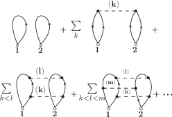
The sum of these diagrams is needed for two important reasons. We need to sum the entire series in order to obtain the correct behavior in low density limit. Second we need the entire series in order to obtain the correct classical limit at high temperature. To understand the latter, consider for simplicity the case of fixed number of time-slices and the expression for $Z$ given by Eq. 13. When the temperature is high, the world-line of any particle collapses to a point: this can be realized mathematically by noticing that the world-line is made up of the product of the Gaussians of the form given by Eq. 11 and as the temperature becomes high, $\delta\tau=\hbar\beta/M\to 0$, these Gaussians approach a delta-function of the difference in the two positions of the particle at two successive imaginary-time slices. In this case, the integrations over $\vec{r}^{(k)}_{i}$ for all $k\neq 0$ in Eq. 13 can be carried out. This eliminates all the integrals corresponding to the coordinates $\vec{r}^{(k)}_{i}$ for $k\neq 0$, and sets $\vec{r}^{(k)}_{i}=\vec{r}^{(0)}_{i}$ for $k\neq 0$ in the integrand, thus, $Z$ contains just $N$ integrals over the $N$-particle coordinates $\vec{r}^{(0)}_{i}$:

$${Z\over{Z_{0}}} = \int\prod_{n=1}^{N}\frac{d^{3}r_{n}^{(0)}}{V}\prod_{i<j}(1+h_{ij}^{(0)})^{M}.$$ (45)

Notice that, using the definition of $h^{(0)}_{ij}$ (Eq. 10) the above factor becomes

$$(1+h_{ij}^{(0)})^{M}=e^{-\beta v(r^{(0)}_{ij})},$$ (46)

i.e., we recover the classical partition function. However, since this product has been expanded to obtain the cluster expansion in the quantum case, i.e.,

$$e^{-\beta v(r^{(0)}_{ij})}=(1+h^{(0)}_{ij})^{M}=\sum_{k}\Bigl{(}\begin{array}[]{c}M\\ k\end{array}\Bigr{)}(h^{(0)}_{ij})^{k},$$ (49)

it implies that diagrammatically the collapse of the world-line leads to multiple $h$-lines connecting any two particles at the coordinates which correspond to the initial time. Fig. 10 shows this diagrammatically for the case of $M=3$.

Figure 10: Collapse of quantum world-line in the high temperature limit. The diagram on the left is also an example of a ladder diagram.

In Fig. 11 we show the fate of the series of the zeroth-order diagrams of Fig. 9 in the high-temperature limit.

Figure 11: The fate of the series of the zeroth-order diagrams of Fig. 9 in the high-temperature limit.

This explains the importance of including all zeroth-order diagrams in our formalism. The sum $g_{0}(r_{12})$ of the zeroth-order diagrams contributing to $g(r)$, i.e., those in Fig. 9, defines an effective potential $v_{e}(r)$ as follows:

$$g_{0}(r_{12})=\exp\bigl{(}-\beta v_{e}(r_{12})\bigr{)}.$$ (50)

In order to justify this definition, first, notice that the bare potential is obtained from the high-temperature (classical) and zero-density limit of the distribution function, which is given as:

$$\lim_{\beta\to 0}g_{0}(r_{12})=\exp\bigl{(}-\beta v(r_{12})\bigr{)}.$$ (51)

Also, the high temperature limit of the sum presented in Fig. 9 is the sum given in Fig. 11. The latter sum is equal to the result given by the above Eq. 51 This implies that in the above definition the effective potential corresponds to the case where instead of freezing the particles coordinates at their initial values, which would lead to the classical limit, we allow them to fluctuate in imaginary-time. In the zero-density limit, there are only the world-lines of the two external particles that matter.

The calculation of the sum of all zeroth-order diagrams can be done easily by noting that the diagonal part of the exact two body density matrix is directly proportional to the sum of all the zeroth-order diagrams in the density expansion of $g(r)$. This is true provided that sufficiently large number of time slices have been used to find the sum. This sum can be calculated by using the matrix squaring methodCeperley and Pollock (1992); Klemm and Storer (1973) for the two-body density matrix. The exact two-body density matrix at any temperature can be calculated by starting from the exact two-body density matrix at a very high temperature and then using the matrix squaring method to obtain the exact density matrix at lower temperature.

(b) First Order: Unlike the zeroth-order diagrams the higher order ladder diagrams for an arbitrary number of time slices are harder to calculate. Examples of diagrams which are first order in $\rho$ are shown in Fig. 12. We expect that such an expansion up to first order in $\rho$ will only give accurate results in the low density regime and also in the high temperature regime.

Figure 12: Fig. (a) and Fig. (b) are examples of $1^{st}$ (in $\rho$) order ladder diagrams.

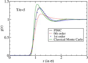
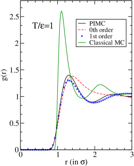
To compare the first order correction against the PIMC we have used only two time slices but using the $v_{eff}(r)$ instead of the bare interaction calculated at $\beta/2$. Using this approach we calculated $g(r)$ at both low temperature ($T=1$) and at high temperature ($T=5$) and for helium density $\rho=0.365\sigma^{-3}$. As we discuss in Appendix B, while the effective interaction provides a good approximation for low-density for $M=1$, when the value of $M$ is increased, the effective interaction approach yields results which at first diverge from the exact solution at low $\rho$. On the contrary, for helium density $\rho=0.365\sigma^{-3}$, the $g(r)$ obtained for $M=2$ using the effective interaction in the PIMC simulation is close to that corresponding to the $M\to\infty$ limit. In the Fig. 13 and Fig. 13 we compare the calculated $g(r)$ with the results of PIMC. This approximation surprisingly yields results for $g(r)$, which, in general, agree with the PIMC results at smaller distances at both low and high temperature. As expected, the agreement with Monte Carlo is better when the temperature is high.

Figure 13: Comparison of the calculated $g(r)$ within zeroth order (red dashed-line) and first order (blue circles) with the results of our PIMC simulation (black-line) for $T/\epsilon=5$ (panel (a)) and $T/\epsilon=1$ (panel (b)). The green solid-line is the result of classical Monte Carlo simulation.

VI.2 Quantum Hypernetted Chain Equations (QHNC)

Next, we will attempt to find the equations which will allow us to resum the diagrams contributing to $g(r)$ by generalizing the classical HNC approach to the quantum case. In order to achieve this, we begin by first classifying the diagrams as nodal ($N$) diagrams or as non-nodal (or composite) ($X$) diagrams (this is similar to the classical caseHiroike (1957a, b); Morita (1958, 1959); Morita and Hiroike (1961); Morita (1960); Morita and Hiroike (1960)) and we ignore the elementary diagrams. We make use of the fact that any nodal diagram is either a convolution of a non-nodal diagram with another non-nodal diagram or a convolution of a non-nodal diagram with a nodal diagram. To be able to sum all the diagrams which contribute to $g(r)$ we will need to consider convolutions of auxiliary diagrammatic pieces which do not necessarily contribute to $g(r)$ by themselves directly, but only through convolution with other diagrams or sub-diagrams. Such sub-diagrams can have external points which can be extremities of only $h$ lines or there can also be sub-diagrams in which one or both of their external points lie on the path of an $L$-line. Because of this, we further divide the class of the $N$ and $X$ diagrams into sub-groups, $N_{\alpha\beta}$ and $X_{\alpha\beta}$ where $\alpha$ and $\beta$ take the values $h$ or $w$ depending on whether the external point is an extremity of just $h$ lines or the external point lies on the path of an $L$-line. This is formally somewhat similar to the case of the so-called Fermi HNC (FHNC) Fantoni and Rosati (1975); Manousakis et al. (1983) equations technique, which was applied to calculate ground-state expectation values with Jastrow-Slater variational wavefunctions. In our case, however, unlike the case of FHNC, we need to further divide the nodal and composite diagrams into sub-groups of equal-time and unequal-time diagrams. Next, we outline the definitions of various sub-groups in detail as follows:

1. $N_{hh}$ or $X_{hh}$ diagrams: In these type of diagrams the two external points $\vec{r}_{1}^{(k)}$ and $\vec{r}_{2}^{(l)}$ are connected by $h$-lines. When $k$=$l$, these diagrams are at equal time and are denoted by $N_{hh}^{(k)}(r_{12})$ and $X_{hh}^{(k)}(r_{12})$. When $k\neq l$, these are unequal-time diagrams and are denoted by $N_{hh}^{(kl)}(r_{12})$ (or $X_{hh}^{(kl)}(r_{12})$). Some examples are shown in Fig. 14:

Figure 14: (a) An example of equal-time $N_{hh}$ diagram. (b) An example of a unequal-time $N_{hh}$ diagram. (c) An example of an equal-time $X_{hh}$ diagram. (d) An example of a unequal-time $X_{hh}$ diagram.

2. $N_{hw}$ or $X_{hw}$ type diagrams: In these type of diagrams the external point $\vec{r}_{1}^{(k)}$ is connected by only $h$-lines and the external point $\vec{r}_{2}^{(l)}$ lies on a $L$-line. When $k$=$l$, these are equal time diagrams and are denoted by $N_{hw}^{(k)}(r_{12})$ (or $X_{hw}^{(k)}(r_{12})$). When $k\neq l$, these are unequal-time diagrams and are denoted by $N_{hw}^{(kl)}(r_{12})$ (or $X_{hw}^{(kl)}(r_{12})$). In a similar way we can have $N_{wh}$ or $X_{wh}$ type of diagrams. Some examples are shown in Fig. 15.

Figure 15: (a) An example of equal-time $N_{hw}$ diagram. (b) An example of a unequal-time $N_{hw}$ diagram. (c) An example of an equal-time $X_{hw}$ diagram. (d) An example of a unequal-time $X_{hw}$ diagram.

3. $N_{ww}$ or $X_{ww}$ diagrams: In these type of diagrams the two external points $\vec{r}_{1}^{(k)}$ and $\vec{r}_{2}^{(l)}$ lie on $L$-lines. When $k$=$l$, these are equal time diagrams and are denoted by $N_{ww}^{(k)}(r_{12})$ (or $X_{ww}^{(k)}(r_{12})$). When $k\neq l$ these are unequal-time diagrams and are denoted by $N_{ww}^{(kl)}(r_{12})$ (or $X_{ww}^{(kl)}(r_{12})$). Some examples are shown in Fig. 16.

Figure 16: Fig. (a) shows an example of equal time $N_{ww}$ diagram. Fig. (b) shows unequal-time $N_{ww}$ diagram. Fig. (c) shows an example of equal time $X_{ww}$ diagram. Fig. (d) shows unequal-time $X_{ww}$ diagram.

Next, a set of self-consistent closed equations for various $X$ and $N$ type of diagrams can be written. Any $N_{hh}$ type diagram can be generated as a convolution of $hh$ type diagram with another $hh$ type diagram or with an $wh$ type diagram. Similarly, a $N_{wh}$ type of diagram may be constructed as a convolution of a $wh$ type diagram with another $wh$ type diagram or from a $ww$ type of diagram with a $hh$ type diagram. Finally, $N_{ww}$ type of diagram may be obtained as a convolution of (a) a $ww$ type with a $hw$ type diagram or (b) a $wh$ type with a $hw$ type diagram, or (c) a $wh$ type with a $ww$ type diagram. The basic rule involved in writing these equations is that any two points can only be convoluted if at least one of them is of $h$-type. In a similar fashion we can see that an unequal-time diagram can be generated by taking convolution of two unequal-time diagrams or a convolution of an equal time diagram with an unequal-time diagram. The generalized equations for any type of nodal diagram are given below:

$$N_{\alpha\beta}^{(kl)}(r_{12}) = \rho\overset{M-1}{\underset{m=0}{\sum}}\underset{\gamma,\gamma^{\prime}}{\sum}^{\prime}\int X_{\alpha\gamma}^{(km)}(r_{13})(X_{\gamma^{\prime}\beta}^{(ml)}(r_{32})+$$ (52)

$$N_{\gamma^{\prime}\beta}^{(ml)}(r_{32}))d^{3}\vec{r}_{3}^{(m)}.$$

Here, the subscripts $\alpha,\beta,\gamma$ and $\gamma^{\prime}$ can be either $w$ or $h$ and the presence of $\sum^{\prime}$ means that the sum over the $\gamma$ and $\gamma^{\prime}$ indices is constrained such that (as explained before) $\gamma$ and $\gamma^{\prime}$ both can not be $w$ simultaneously. The unequal-time $X$-type of diagrams can be written in terms of the unequal-time nodal diagrams in the following way:

$$X_{hh}^{(kl)}(r_{12})=e^{N_{hh}^{(kl)}(r_{12})}-N_{hh}^{(kl)}(r_{12})-1,$$ (53)

$$X_{hw}^{(kl)}(r_{12}) = e^{N_{hh}^{(kl)}(r_{12})}N_{hw}^{(kl)}(r_{12})-N_{hw}^{(kl)}(r_{12}),$$ (54)

$$X_{ww}^{(kl)}(r_{12}) = e^{N_{hh}^{(kl)}(r_{12})}[N_{ww}^{(kl)}(r_{12})+N_{hw}^{(kl)}(r_{12})N_{wh}^{(kl)}(r_{12})]$$ (55)

$$+ \frac{1}{\rho V_{\theta}}l(r_{12},\tau_{kl})\cdot l(r_{12},\theta-\tau_{kl})$$

$$- N_{ww}^{(kl)}(r_{12}).$$

In the above equations $\tau_{kl}$ is the time interval between the $k^{th}$ and $l^{th}$ time slices and the function $l$ is defined as follows:

$$l(r_{12},\tau_{kl}) = \frac{1}{\lambda^{3}_{\tau_{kl}}}\exp\Bigl{[}{-\pi\frac{(\vec{r}_{1}^{(k)}-\vec{r}_{2}^{(l)})^{2}}{\lambda^{2}_{\tau_{kl}}}}\Bigr{]}.$$ (56)

The equal time $X$-type of diagrams can be written in terms of the equal time nodal diagrams in the following way:

$$X_{hh}^{(l)}(r_{12}) = f(r_{12})e^{N_{hh}^{(l)}(r_{12})}-N_{hh}^{(l)}(r_{12})-1,$$ (57)

$$X_{hw}^{(l)}(r_{12}) = f(r_{12})e^{N_{hh}^{(l)}(r_{12})}N_{hw}^{(l)}(r_{12})-N_{hw}^{(l)}(r_{12}),$$ (58)

$$X_{ww}^{(l)}(r_{12}) = f(r_{12})e^{N_{hh}^{(l)}(r_{12})}[N_{ww}^{(l)}(r_{12})+N_{hw}^{(l)}(r_{12})$$ (59)

$$\times N_{wh}^{(l)}(r_{12})]-N_{ww}^{(l)}(r_{12}),$$

$$f(r_{12}) = 1+h(r_{12})=e^{-{{\delta\tau}\over{\hbar}}v(r_{12})}.$$ (60)

By solving these equations we can find the numerical values of all the nodal diagrams and then use them to find the pair distribution function. The pair distribution can be written in the following way in terms of the nodal functions:

$$g(r_{12})= f(r_{12})e^{N_{hh}^{(0)}(r_{12})}(1+N_{ww}^{(0)}(r_{12})+$$ (61)

$$2N_{hw}^{(0)}(r_{12})+N_{hw}^{(0)}(r_{12})N_{wh}^{(0)}(r_{12})).$$

VI.3 Implementation of QHNC

VI.3.1 Effective interaction approach

In our QHNC equations we used the effective interaction obtained from the exact two-body density matrix instead of the bare interaction. Namely, instead of $h^{(k)}_{ij}$ we use an effective $h$-line, i.e., the $h^{(k)}_{ij}$ obtained from Eq. 10 using $v_{e}(r)$ (given by Eq. 50) instead of the bare interaction.

There are two ways to justify the use of the effective interaction instead of the bare.

A) Using the exact two-body density-matrix (ETBDM) as starting point: We note that we could have defined our original starting point, such that, instead of using the bare interaction in Eq. 10 to use the effective potential. This effective $h$, i.e., $h_{e}$ and the bare $h$ are the same to order $\delta\tau$. This is what is done in most PIMC studiesPollock and Ceperley (1984); Ceperley and Pollock (1986); Pollock and Ceperley (1987); Ceperley and Pollock (1989, 1992) of liquid ⁴He. Therefore, since we need to make sure that the process converges by taking the $M\to\infty$ limit, both potentials should yield the same limit. The effective potential corresponds to using the ETBDM in the two-body Trotter break-up of the operator $e^{-\delta\tau\hat{H}/\hbar}$ which leads to using our effective potential in Eq. 10. The reason to prefer the effective potential as a starting point, is our hope that it will lead to a faster convergencePollock and Ceperley (1984) with respect to $M$.

B) Using the primitive Trotter approximation (PTA) as starting point: This means that we simply begin our cluster expansion or the PIMC simulation starting from the bare interaction in Eq. 10. In this approach the effective interaction emerges as the zero-density limit or by retaining just the two-body clusters. Furthermore, even if we start from the PTA as a starting point, this effective interaction should be incorporated in the QHNC equations, because they do not account for diagrams such as those in Fig. 9 which contain more than two $h$-lines. As discussed in Sec. VI.1 the inclusion of all the diagrams shown in Fig. 9 is necessary to obtain the correct classical limit and low density limit.

The reason that we have the choice between A and B is because of the fact that $M$ and $\delta\tau$ are tunable. However, there are different issues with both using the ETBDM or the PTA as starting points to justify the use of the effective interaction. If we use PTA as starting point, the effective interaction is derived as the zero density limit. Within this approach, if we simply replace the $h$-line with an effective $h$-line it can lead to a consistency problem which is discussed in the next subsections. If we start from the ETBDM, there is no such conceptual issue with justifying its use; however, as we will see in the next two subsections, there is a different issue which arises with the convergence with $M$ of the PIMC method in the low-density regime.

In the next subsection, we have solved the QHNC equations, using the effective potential for the case of $M=1$ and $M=2$, to find the pair distribution function for our test system.

VI.3.2 Calculation with $M=1$:
Two-body mean-field approximation.

It is easy to see that, when $M=1$, our QHNC equations transform into the classical HNC equations. This happens because all the un-equal time functions become zero and the equations take a simple form where only equal time $hh$ functions survive.

Figure 17: Illustration of an effective interaction picture which emerges at low density and in the high temperature limit using the ring-polymer isomorphism. The color denotes the various positions of the atoms at different time-slices. The solid lines denote the $L$-lines, i.e., the spring-like interactions in the classical ring-polymer picture of the many-body path integral. The dashed-lines denote the interaction between each bead of the polymer with the corresponding bead of another polymer at the same time-slice.

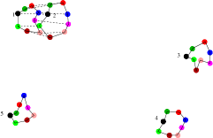
While we still work within the PTA starting point approach, we will use the effective potential in conjunction with the HNC. One might question that such an effective-HNC approximation can be appropriate for a quantum problem. First, note that the effective potential (see discussion in Sec. VI.1) takes into account the effect of the presence of world-lines in a way which is exact in the zero-density limit. Therefore, it should be expected to be a good approximation in the low-density regime also. Furthermore, in the high-temperature limit we obtain the classical partition function and, as a result, the HNC approximation is the appropriate treatment and is known to be accurate for a wide density range.

Our $M=1$ approximation should be viewed as a two-body mean-field theory, which is a consistent theory, and it should not be considered as just the simple one time-slice approximation. Namely, the physical meaning of the approximation is that we account for all the quantum effects at the two-body level exactly, and this defines an effective integration which can be treated with classical statistical mechanics. In Fig. 17 we illustrate the nature of the approximation. At low density the most probable configurations are the ones with mostly monomer configurations (ring-polymers with distance from the other ring-polymers beyond the interaction range). The next most probable occurrences are the clusters of two ring-polymers. A treatment in which only the ring-monomers are considered leads to the non-interacting ideal gas approximation. The next level is to consider the two-body clusters and to solve the two-ring polymer problem exactly by summing up all interaction terms using an infinite number of times-slices. This solution defines the effective interaction discussed in Sec. VI.1, which is then used to take into account the interaction of the center of mass of these ring-polymers.

Notice that in the low density limit this treatment should be a good approximation. A second condition for this approach to be accurate is that the amplitude of the quantum-thermal fluctuations of the particle positions, as captured by the de Broglie wavelength $\lambda_{\hbar\beta}$, should be small as compared to $r_{s}$ ($(4/3)\pi r_{s}^{3}\rho=1$), i.e.,

$$r_{s}>>\frac{\hbar}{\sqrt{2\pi mk_{B}T}}.$$ (62)

This is the analogue to the Born-Oppenheimer approximation which separates the fast from the slow degrees of freedom. Here, we integrate out the degrees of freedom at all intermediate time-slices for each pair of atoms. Therefore, a third condition for the applicability of this approach is that the time-scale for a third particle to approach an interacting pair and influence it, should be much larger than the imaginary-time $\theta=\hbar\beta$. This implies that $r_{s}/v_{th}>>\theta$, where $v_{th}$ is the classical atomic thermal velocity, and this leads to the condition:

$$r_{s}>>\frac{\hbar}{\sqrt{3mk_{B}T}}.$$ (63)

Notice that Eq. 63 and Eq. 62 are compatible with each other, giving approximately the same density-temperature boundary for the validity of this approximation. Notice that this condition is very well satisfied for the case of liquid ⁴He at temperature of the order of $T/\epsilon\sim 1$.

Figure 18: Comparison of $g(r)$ for particles interacting with Lennard-Jones potential for density $\rho=0.365\sigma^{-3}$ and for temperature (a) $T/\epsilon=5$ and (b) $T/\epsilon=1$. The black solid-line is the result obtained from our PIMC simulation extrapolated to $M\to\infty$ and $N\to\infty$. The blue circles represent the result obtained by using the QHNC equations for $M=1$.

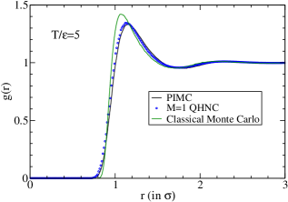
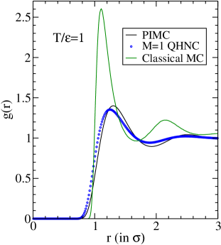
In an approach where we begin from the PTA as starting point, it appears that when we use the effective $h$-line in the QHNC equations it produces spurious diagrams in which a particle has two world-lines. However, these diagrams require a third particle to be in close proximity with the two external particles. However, at low density, the probability for that to occur is low. At high and moderately low temperature, this can be also justified and a detailed discussion has been provided in Appendix A.

In order to test the accuracy of this scheme we have applied it to the case of ⁴He as described by the Lennard-Jones interaction. Results have been obtained for a rather high-density using $\rho=0.365\sigma^{-3}$ (the zero temperature liquid ⁴He equilibrium density). The matrix squaring method has been used to obtain the effective $h$-line at two different temperatures namely $T=5$ and $T=1$ (see Fig. 18 and Fig. 18 for results). Notice that the results are reasonably close to those obtained by PIMC using large enough number of time-slices to achieve convergence. We note that the agreement between the $M=1$ approximation and the exact results improves as the density is decreased or the temperature is increased.

VI.3.3 Calculation with $M=2$

Within the PTA approach, i.e., starting from the expression of the path-integral with the bare interaction, there is an inconsistency in replacing the bare interaction with the effective interaction for $M>1$. This does not present a conceptual problem when one starts with the ETBDM approachCeperley and Pollock (1992) because this interaction is our starting point. However, surprisingly, as illustrated in Appendix B, while the use of the effective interaction with $M=1$ is exact at zero-density and close to the exact at low-density, when the value of $M$ is increased, the effective interaction approach yields results which at first diverge from the exact solution at low $\rho$ and it takes high values of $M$ to achieve convergence. Therefore, since we need to achieve convergence with respect to the number of time slices $M$, the PTA approach is superior to the the ETBDM approach. This is demonstrated in Appendix B.

Figure 19: (a) Convergence of $g(r)$ with the number of time-slices $M$ obtained at density of 0.365 $\sigma^{-3}$ starting from the bare interaction and with effective interaction as a starting point and carrying a PIMC simulation. (b) Same as in (a) by expanding the scale near the $g(r)$ maximum for clarity.

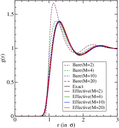
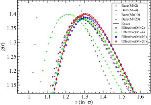
On the contrary at densities of the order of ⁴He equilibrium density, i.e., at density 0.365 $\sigma^{-3}$, the $g(r)$ obtained for $M=2$ using the effective interaction in the PIMC simulation is close to that corresponding to the $M\to\infty$ limit. Fig. 19 (Fig. 19 for more detail near the main peak of $g(r)$) shows our results obtained with the PIMC method as a function of the number of time-slices $M$ starting from either the bare interaction or the effective interaction. Notice that in fact the results for $M=2$ when using the effective interaction are not too far from $M=\infty$. On the contrary when starting from the PTA we need to use $M=20$ to achieve the same level of convergence. This also allows us to work with a few time slices without compromising the accuracy of the results for such densities. Furthermore, as shown in Sec. VI.1, when we calculated the first order correction to $g(r)$ with just two time slices but using the effective interaction, the results were reasonably good for at least the high temperature case.

In Fig. 20 we compare the results for $g(r)$ obtained by using the effective potential obtained after matrix squaring in conjunction with our QHNC equations with $M=2$. Notice that the results of using QHNC are in some disagreement with the results of PIMC.

Figure 20: Comparison of $g(r)$ between PIMC (solid line) and the QHNC (dashed line) with $M=2$ for temperature $T/\epsilon=1$ (red) and $T/\epsilon=5$ (blue).

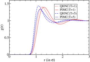
We would like to emphasize that our QHNC equations fail to include ladder diagrams and the other diagrams that would be produced by involving such ladder diagrams in Eq. 52. Such diagrams which are of zeroth order were included by using the effective potential as discussed in the previous subsection for $M=1$. In addition, the QHNC equations miss ladder diagrams where the ladder is formed by connecting via $h$-lines parts of world-lines of different particles to construct the steps of the ladder (spatial-ladders). Including the exact contribution of such ladder diagrams is not an easy task.

Here, we outline a modification of the QHNC approach which allows us to include an approximation of all such ladder diagrams. In the regime where the contribution of such diagrams is small, a good estimate of their contribution could provide an accurate enough calculation.

1) We begin by using the QHNC equations to obtain the pair distribution function using the effective potential for $\delta\tau=\hbar\beta/2$ (obtained by using the matrix squaring method) because we are dealing with $M=2$.

2) Next, we approximate these missing diagrams.

First, imagine that we have summed up all the diagrams contributing to $g(r)$ (with the exception of the elementary diagrams) and the expression is given by the functional $g(\{L\},\{h\})$. Namely, we would like to consider the sum of all the diagrams contributing to $g$ as a functional of the $L$-lines and the $h$-lines for a reason that will become clear below. To be consistent, the solution to the QHNC equations will be given by $g_{Q}(\{L\},\{h\})$, where $h$ is the $h$-line which corresponds to the effective potential. Then, the contribution of the missing diagrams is given by

$$\Delta g=g(\{L\},\{h\})-g_{Q}(\{L\},\{h\}).$$ (64)

Since the $\Delta g$ shown in Fig. 20 is small compared to $g(r)$ itself we will approximate $\Delta g$, i.e., the contribution of the missing diagrams by using their simplified expressions at high-temperature. As we have discussed previously, when $\delta\tau$ is small, the $L$-lines are Gaussian approximations to the delta-function, and in the limit of $\delta\tau\to 0$ they are true delta-functions leading to the classical limit, by “collapsing” the world lines in any given diagram. Therefore, a high-temperature approximation of these missing diagrams is given by

$$\Delta g=g(\{\delta\},\{h\})-g_{Q}(\{\delta\},\{h\}).$$ (65)

$g(\{\delta\},\{h\})$ and $g_{Q}(\{\delta\},\{h\})$ are, respectively, the expression of the exact distribution function and that obtained by solving the QHNC equations by replacing the $L$-lines, with a delta-function.

However, as we have shown in Sec. VI.1 $g(\{\delta\},\{h\})=g_{cl}$; namely if we start from the sum of all the diagrams and we replace the $L$-lines by a $\delta$-function, we obtain the classical limit. As a result the contribution of the missing ladder diagrams from the QHNC equations can be approximated by

$$\Delta g=g_{cl}-g_{Q}(\{\delta\},\{h\}).$$ (66)

Here, $g_{cl}$ is the pair distribution function obtained by using the classical HNC. The fact that the HNC contains the high temperature approximation of the missing ladder diagrams is demonstrated diagrammatically in Fig. 21. The reader can understand the above statement by studying Fig. 21 (and its caption) in conjunction with our discussion of Sec. VI.1.

Figure 21: (a) A ladder diagram contributing to full distribution function $g$ which is not obtained by the QHNC equations. In the high-temperature limit the diagram (a) reduces to diagram (b) because of the “collapse” of the world-lines. This diagram is contained in the classical HNC diagram shown in (c) in which the bold-dashed line is expressed in terms of the $h$-lines in the series illustrated in (d).

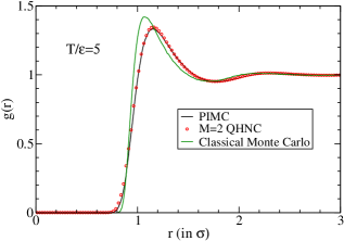
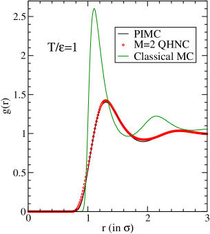
We worked at density 0.365$\sigma^{-3}$ using two values of temperature, $T/\epsilon=1$ and $T/\epsilon=5$, and the calculation of $g(r)$ is implemented as follows. For example, when using $T/\epsilon=5$, we first obtained the $h_{eff}(T)$ at $T/\epsilon=10$ and we used it in the QHNC equations to obtain $g_{Q}$. Then, we used this $h_{eff}(10)$ to obtain $g_{Q}(\{\delta\},\{h\})$. The effective $h$ given by

$$h_{eff}={(h_{eff}(10)+1)}^{2}-1,$$ (67)

was used in the classical HNC equations to obtain $g_{cl}$. Fig. 22 and Fig. 22 illustrate our results for $T/\epsilon=5$ and $T/\epsilon=1$ and compares them to the results obtained from PIMC simulation for $M\to\infty$. We can clearly see in Fig. 22 that the results from QHNC with $M=2$ (with the correction of $\Delta g$ described above given by Eq. 66) agree with the exact PIMC simulation. Fig. 22 for $T/\epsilon=1$ indicates that the QHNC equations with $M=2$ (with the correction of $\Delta g$ given by Eq. 66) yields more accurate than the QHNC with $M=1$.

Figure 22: Comparison of $g(r)$ obtained by adding the high-temperature approximation $\delta g$ to the QHNC results for $M=2$ (red circles) for density $\rho=0.365\sigma^{-3}$ and for temperature (a) $T/\epsilon=5$ and (b) $T/\epsilon=1$ to the PIMC simulation extrapolated to $M\to\infty$ and $N\to\infty$ (black-solid line).

VI.3.4 Calculation with larger values of $M$

If we apply the QHNC approach for $M>2$ we find that the results do not agree very well with the PIMC simulation. The QHNC equations fail to include diagrams in which world-lines involving more than one instant of imaginary time where an interaction $h$-line occurs. These are diagrams which appear as ladders in the time direction (time-ladders). These diagrams begin to occur for $M>2$. In addition, the QHNC equations miss ladder diagrams where the ladder is formed by connecting parts of world-lines of different particles to construct the steps of the ladder (spatial-ladders).

There are ways to generalize the QHNC equations to include such diagrams similar in spirit to those techniques used in conventional many-body perturbation theoryBethe and Salpeter (1951) and this is one of the directions of our future work.

VII Conclusions

We have revived the old well-known method of cluster-expansion in classical statistical mechanicsMayer and Mayer (1940) by extending its application to the many-body path integral and we have derived a diagrammatic expansion for the pair distribution function. The diagrammatic expansion for the pair distribution function contains both connected and some factorizable/disconnected diagrams. These disconnected diagrams which do not cancel exactly involve disconnected parts with common particles and can be paired with co-contributing factorizable diagrams or some non-factorizable connected diagrams contributing with an opposite sign. Because of this “pairing”, these paired diagrams almost cancel and it can be shown that the cancellation is exact in the high-temperature limit. By ignoring the contribution of these diagrams we can derive a cluster expansion of connected diagrams which can be written as a formal power series expansion in the particle density $\rho$. The series can be also thought of as an expansion where we keep all diagrams involving up to $n$-body clusters. We compared our results to results we obtained by applying the PIMC technique which is exact for distinguishable particles. Surprisingly, the calculation of $g(r)$ including up to three-body diagrams (first order in $\rho$) gives results for the Lennard-Jones system which are accurate even for liquid-⁴He equilibrium densities and for temperature $T/\epsilon=1$ where $\epsilon$ is the well-depth of the Lennard-Jones potential.

We also generalized the hypernetted-chain approximation for our quantum mechanical case (QHNC). We solved the QHNC equation for the Lennard-Jones system for the case of one ($M=1$) and two ($M=2$) imaginary-time slices along with an effective potential obtained from the matrix squaring technique. This was found to be accurate down to moderately low temperature ($T/\epsilon=1$). We find that our QHNC equations need to be generalized to tackle the case of $M>2$.

Our method is generalizable to the case of identical particles and in particular to the case of fermions. We hope that this method can provide useful results to compare with the results obtained by applying quantum Monte Carlo (QMC) methods in this latter case where the QMC results are not exact. We hope to provide results for this case in the near future.

VIII Acknowledgments

This work was supported in part by the U.S. National High Magnetic Field Laboratory, which is funded by NSF DMR-1157490 and the State of Florida.

Appendix A Spurious diagrams

In the effective-HNC approximation (i.e., our $M=1$ approximation) the terms up to zeroth order match exactly with the exact quantum expansion up to zeroth order. However, for terms which are higher than zeroth order, the effective-HNC approximation is not able to account for all the terms that appear in the exact quantum expansion. There are spurious terms which appear in the expansion in which the particles have two world-lines (see Fig. 23).

Figure 23: Examples of spurious terms that appear in effective HNC expansion in which particle 3 appears to have two world-lines.

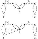
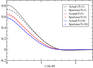
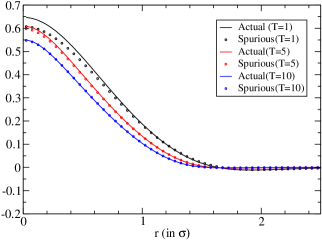
The high-temperature limit of the effective $h$-line is the classical $h$-line. Also, both the exact quantum pair distribution function and the pair distribution function obtained from effective-HNC become the classical pair distribution function in the high-temperature limit. For any spurious diagram that appears in the effective-HNC there is a unique counterpart diagram in the exact expression for $g(r)$ (see Fig. 24 as an example).

Figure 24: (a) A term that appears in the exact quantum expansion. (b)The spurious counterpart of (a) in which particle labeled 3 appears to have two world-lines.

Any such spurious diagram and its counterpart in the actual expansion have approximately the same contribution in certain temperature regime (as temperature becomes high the two match exactly). We have compared the two terms (exact and its spurious counterpart) that appear in Fig. 24 for different temperature to see how close these two terms are down to temperature $T/\epsilon=1$. We kept the number of time slices fixed at 16 and have considered the case where $k=l=1$ and the case where $k=1$ and $l=4$. The results are shown in Fig. 25, and Fig. 26.

Figure 25: Comparison of the exact term and its spurious counterpart for the case where $k=l=1$. The total number of division used is 16 ($M=16$)

Figure 26: Comparison of the contributions of the exact diagram and that of its spurious counterpart for the case where $k=1$ and $l=4$ for $M=16$.

Since the expansion parameter is $\rho$ we expect the effective-HNC scheme to be more accurate in the low density and high temperature regime.

Appendix B Convergence with respect to the number of time-slices $M$

The approach of using the ETBDM in PIMC simulations and in our approach has the following problem for low density illustrated in Fig. 27 for zero density. Fig. 27 presents the results obtained for $g(r)$ for various values of $M$ using (a) the bare interaction and (b) the effective interaction corresponding to the particular value of $M$. It can be clearly seen that when we use the bare interaction the results for $M=20$ are very close to the exact results. When, however, we use the effective interaction, even though the $g(r)$ for $M=1$ is already the exact $g(r)$, the results for $M=2,3,4,5$ move further away from exact solution and, for larger values of $M$, they begin moving closer to the exact solution. However, even for $M=20$ they are still far from the exact results. Therefore, the convergence is faster when the bare interaction is used. Thus, if one did not know that the starting $g(r)$, which corresponds to $M=1$ was the exact solution, and one uses the convergence criterion to extract the correct $g(r)$ it is better to use the bare interaction, i.e., the approach based on the PTA. This creates a problem for the convergence with $M$ in the PIMC approach at low density when starting from the ETBDM. While this seems surprising at first, it can be easily understood within our approach. While the effective potential for $M=1$ corresponds to the exact $g(r)$ at zero density (and presumably a good approximation at low density), when dealing with $M>1$ using the effective potential corresponding to inverse temperature $\beta/M$ for the $M$ intermediate time-slices leads to the following problem. The density sub-matrix needed to connect two consecutive time-slices separated by $\delta\tau=\hbar\beta/M$ is the full density matrix including its off-diagonal matrix elements in order to connect the points at $\vec{r}_{1}^{(M)},\vec{r}_{2}^{(M)}$ with the points $\vec{r}_{1}^{(M+1)},\vec{r}_{2}^{(M+1)}$. Instead, only the diagonal matrix elements are utilized when we use the effective potential. This yields the correct $g(r)$ when $M$ is infinite and in that limit the bare interaction is good enough. This leads to the results presented in Fig.  27 where, if we use the effective interaction, the density matrix is already the exact at the $M=1$ level, and by trying to go beyond that by increasing the value of $M$, using the effective interaction at $M>1$, the results first diverge from the exact results and, then, slowly approach the same solution after very large value of $M$ (see Fig. 27).

Figure 27: (a) Convergence of $g(r)$ with the number of time-slices $M$ obtained at zero-density starting from the bare interaction, i.e., within the PTA approximation and with the ETBDM (effective interaction) as a starting point. (b) Convergence of the maximum of $g(r)$ as a function of $M$ with the two approaches.

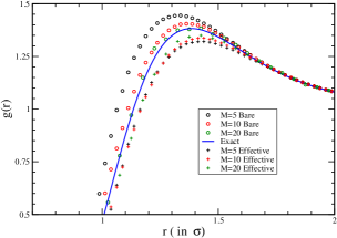
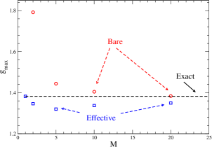
On the contrary at densities of the order of ⁴He equilibrium density, i.e., at density 0.365 $\sigma^{-3}$, the convergence when using the effective interaction is much better than when using the bare interaction as starting point. This is illustrated in Fig. 19, which is the same as Fig. 19 but we have expanded the region near the peak. We can now clearly see that for this high density using the effective interaction we achieve much faster convergence with $M$ as compared to using the bare interaction.

References

- Mayer and Mayer (1940) J. E. Mayer and M. G. Mayer, Statistical Mechanics (1940) p. Chapt. 13.
- Goodstein (2002) D. Goodstein, States of Matter, Dover Books on Physics Series (Dover, 2002).
- Hiroike (1957a) K. Hiroike, J. Phys. Soc. Jap. 12, 326 (1957a).
- Hiroike (1957b) K. Hiroike, J. Phys. Soc. Jap. 12, 864 (1957b).
- Morita (1958) T. Morita, Prog. Theor. Phys. 20, 920 (1958).
- Morita (1959) T. Morita, Prog. Theor. Phys. 21, 361 (1959).
- Morita and Hiroike (1961) T. Morita and K. Hiroike, Prog. Theor. Phys. 25, 537 (1961).
- Morita (1960) T. Morita, Prog. Theor. Phys. 23, 829 (1960).
- Morita and Hiroike (1960) T. Morita and K. Hiroike, Prog. Theor. Phys. 23, 1003 (1960).
- Prokof’ev and Svistunov (1998) N. V. Prokof’ev and B. V. Svistunov, Phys. Rev. Lett. 81, 2514 (1998).
- Mishchenko et al. (2000) A. S. Mishchenko, N. V. Prokof’ev, A. Sakamoto, and B. V. Svistunov, Phys. Rev. B 62, 6317 (2000).
- Ceperley (1995) D. M. Ceperley, Rev. Mod. Phys. 67, 279 (1995).
- McMahon et al. (2012) J. M. McMahon, M. A. Morales, C. Pierleoni, and D. M. Ceperley, Rev. Mod. Phys. 84, 1607 (2012).
- Zhang et al. (1997) S. Zhang, J. Carlson, and J. E. Gubernatis, Phys. Rev. B 55, 7464 (1997).
- Feynman and Hibbs (1965) R. P. Feynman and A. R. Hibbs, Quantum Mechanics and Path Integrals (McGraw-Hill, New York, 1965).
- Feynman (1998) R. Feynman, Statistical Mechanics: A Set Of Lectures, Advanced Books Classics (Avalon Publishing, 1998).
- Ceperley and Alder (1980) D. M. Ceperley and B. J. Alder, Phys. Rev. Lett. 45, 566 (1980).
- Fetter and Walecka (2003) A. Fetter and J. Walecka, Quantum Theory of Many-particle Systems, Dover Books on Physics (Dover Publications, 2003).
- Bohm and Pines (1953) D. Bohm and D. Pines, Phys. Rev. 92, 609 (1953).
- Pandharipande and Wiringa (1979) V. R. Pandharipande and R. B. Wiringa, Rev. Mod. Phys. 51, 821 (1979).
- Ceperley and Pollock (1992) D. M. Ceperley and E. L. Pollock, Eds S. Caracciolo and A. Fabrocini , ETS Edtrice, Pisa, Italy, pg. 35 (1992).
- Klemm and Storer (1973) A. Klemm and R. Storer, Aust. J. Phys. 26, 43 (1973).
- Fantoni and Rosati (1975) S. Fantoni and S. Rosati, Il Nuovo Cimento A 25, 593 (1975).
- Manousakis et al. (1983) E. Manousakis, S. Fantoni, V. R. Pandharipande, and Q. N. Usmani, Phys. Rev. B 28, 3770 (1983).
- Pollock and Ceperley (1984) E. L. Pollock and D. M. Ceperley, Phys. Rev. B 30, 2555 (1984).
- Ceperley and Pollock (1986) D. M. Ceperley and E. L. Pollock, Phys. Rev. Lett. 56, 351 (1986).
- Pollock and Ceperley (1987) E. L. Pollock and D. M. Ceperley, Phys. Rev. B 36, 8343 (1987).
- Ceperley and Pollock (1989) D. M. Ceperley and E. L. Pollock, Phys. Rev. B 39, 2084 (1989).
- Bethe and Salpeter (1951) H. Bethe and E. Salpeter, Phys. Rev. 84, 1232 (1951).