Revisiting relaxation in globular clusters

Chris Hamilton1,2, Jean-Baptiste Fouvry3, James Binney1, Christophe Pichon4,5,6
1Rudolf Peierls Centre for Theoretical Physics, 1 Keble Road, Oxford, OX1 3NP, UK
2Department of Applied Mathematics and Theoretical Physics, University of Cambridge, Wilberforce Road, Cambridge CB3 0WA, UK
3Institute for Advanced Study, Einstein Drive, Princeton NJ 08540, USA
4Institut d’Astrophysique de Paris and UPMC, CNRS (UMR 7095), 98 bis Boulevard Arago, 75014, Paris, France
5Korea Institute of Advanced studies (KIAS), 85 Hoegiro, Dongdaemun-gu, Seoul, 02455, Republic of Korea
6Institute for Astronomy, University of Edinburgh, Royal Observatory, Blackford Hill, Edinburgh, EH9 3HJ, UK
E-mail: ch783@cam.ac.ukHubble Fellow
Abstract

The classical theory of cluster relaxation is unsatisfactory because it involves the Coulomb logarithm. The Balescu–Lenard (BL) equation provides a rigorous alternative that has no ill-defined parameter. Moreover, the BL equation, unlike classical theory, includes the cluster’s self-gravity. A heuristic argument is given that indicates that relaxation does not occur predominantly through two-particle scattering and is enhanced by self-gravity. The BL equation is adapted to a spherical system and used to estimate the flux through the action space of isochrone clusters with different velocity anisotropies. A range of fairly different secular behaviours is found depending on the fraction of radial orbits. Classical theory is also used to compute the corresponding classical fluxes. The BL and classical fluxes are very different because (a) the classical theory materially under-estimates the impact of large-scale collectively amplified fluctuations and (b) only the leading terms in an infinite sum for the BL flux are computed. A complete theory of cluster relaxation likely requires that the sum in the BL equation be decomposed into a sum over a finite number of small wavenumbers complemented by an integral over large wavenumbers analogous to classical theory.

keywords:
Galaxy: kinematics and dynamics – galaxies: kinematics and dynamics – galaxies: star clusters: general – methods: numerical

1 Introduction

As systems of almost coeval stars, globular clusters have been vital to the development and testing of the theory of stellar structure and evolution. As wonderfully clean dynamical systems that have enough stars to allow precise statistical characterisation but few enough stars to evolve significantly by stellar-dynamical relaxation within a Hubble time, their study has been important for the development of stellar dynamics. Yet notwithstanding intensive study for more than a century, aspects of these system remain mysterious. In particular we don’t understand how or where they formed. Moreover, the efficiency with which gas must have been converted into stars when they formed becomes more surprising as our knowledge of the general star-formation process grows.

In this paper we argue that the dynamical evolution of globular clusters is also less well understood than it should be with a critique of the standard theory of two-body relaxation. Then we re-formulate, in the context of a model globular cluster, the theory of the long-time (secular) evolution of a stellar system using a sophisticated approach that has recently explained the secular evolution of collisionless stellar discs.

The conceptual foundation of the theory of secular evolution is that the system evolves through a series of steady-state solutions of the collisionless Boltzmann equation. By Jeans’ theorem, any such solution can be described by a distribution function (DF) that depends on position and velocity (𝐱,𝐯)𝐱𝐯({\bf x},{\bf v}) only through constants of stellar motion. Since we focus on spherical systems, we know that the system’s mean-field Hamiltonian H=12v2+Φ(𝐱)𝐻12superscript𝑣2Φ𝐱H={\textstyle{1\over 2}}v^{2}+\Phi({\bf x}) admits three action integrals Jisubscript𝐽𝑖J_{i}, and we may assume that at each time the DF takes the form f(𝐉)𝑓𝐉f({\bf J}). On a timescale much longer than the system’s crossing time, small fluctuations of the potential ΦΦ\Phi around the slowly evolving mean spherical form for which the Jisubscript𝐽𝑖J_{i} are the action integrals cause the actions of stars to change, and thus the functional form of f𝑓f to evolve.

The most obvious difference between the real potential ΦN(𝐱)subscriptΦ𝑁𝐱\Phi_{N}({\bf x}) and the spherical approximation for which the Jisubscript𝐽𝑖J_{i} are computed, is the local singularities ΦN(𝐱)Gm/|𝐱𝐱i|similar-tosubscriptΦ𝑁𝐱𝐺𝑚𝐱subscript𝐱𝑖\Phi_{N}({\bf x})\sim-Gm/|{\bf x}-{\bf x}_{i}| near the location 𝐱isubscript𝐱𝑖{\bf x}_{i} of each star. The classical theory of relaxation (e.g. Binney & Tremaine, 2008, chapter 7) is based on the idea that as a star moves through the cluster it is repeatedly scattered by the singularities that lie along its path. Following Chandrasekhar (1943) one calculates as a function of impact parameter b𝑏b and relative velocity the velocity change δ𝐯𝛿𝐯\delta{\bf v} that an encounter causes, and then adds these changes by integrating over impact parameters and relative velocities to obtain diffusion coefficients for the Fokker-Planck equation that describes the diffusion of stars through phase space (Chandrasekhar, 1949):

ft=𝐯(𝚫1f12𝐯[𝚫2f]).𝑓𝑡𝐯subscript𝚫1𝑓12𝐯delimited-[]subscript𝚫2𝑓\displaystyle{\partial f\over\partial t}=-{\partial\over\partial{\bf v}}\cdot\biggl{(}\mbox{\boldmath$\Delta$}_{1}f-{\textstyle{1\over 2}}{\partial\over\partial{\bf v}}\cdot\Bigl{[}\mbox{\boldmath$\Delta$}_{2}f\Bigr{]}\biggr{)}. (1)

Here the first-order diffusion coefficient 𝚫1subscript𝚫1\mbox{\boldmath$\Delta$}_{1} is the average δ𝐯delimited-⟨⟩𝛿𝐯\left\langle\delta{\bf v}\right\rangle of the δ𝐯𝛿𝐯\delta{\bf v}, while the second-order diffusion coefficient 𝚫2subscript𝚫2\mbox{\boldmath$\Delta$}_{2} is obtained by averaging the δ𝐯𝛿𝐯\delta{\bf v} in quadrature.

The calculation is made tractable by neglecting the acceleration caused by the mean-field potential ΦΦ\Phi. That is, one assumes that in the absence of a nearby singularity, the star’s trajectory would be a straight line, and in its presence it is a Keplerian hyperbola. This approximation is only valid when the impact parameter b𝑏b is much less than the distance to the cluster’s centre. The inconvenient truth is that the integral for δ𝐯delimited-⟨⟩𝛿𝐯\left\langle\delta{\bf v}\right\rangle over impact parameters diverges at large b𝑏b, signalling that encounters with distant stars contribute significantly to δ𝐯delimited-⟨⟩𝛿𝐯\left\langle\delta{\bf v}\right\rangle.

Fortunately, the divergence is only logarithmic and the text-book work-around for this conceptual difficulty is to cut the integral off at a distance bmaxsubscript𝑏maxb_{\rm max} comparable to the system’s half-mass radius, and report bmaxsubscript𝑏maxb_{\rm max} through the value of the “Coulomb logarithm”, which is the natural logarithm of the ratio of bmaxsubscript𝑏maxb_{\rm max} to the impact parameter that gives rise to scattering by 90 degrees at the mean relative velocity. The venerable age of this work-around should not blind us to its unsatisfactory nature: the divergence of the integral for δ𝐯delimited-⟨⟩𝛿𝐯\left\langle\delta{\bf v}\right\rangle is no mathematical nicety but reflects a real physical issue – the significant contribution of fluctuations in the potential generated by distant rather than nearby stars (Weinberg, 1993). Clearly these stars do not cause Rutherford-like scattering, and they do not act in isolation. In so far as long-range encounters contribute significantly to the secular evolution of the system, the classical formulation of the problem is flawed.

The purpose of this paper is first to argue that the theory of the secular evolution of globular clusters should be reformulated, second to explain what the reformulated theory looks like, and finally to present a worked example of the reformulated theory in action. In Section 2 we give an order-of-magnitude calculation that implies that relaxation is driven not by individual encounters but by fluctuations in the number of particles in different sub-regions of the system. This conclusion suggests that the self-gravity of the system, which is completely neglected in the traditional approach, can play a significant role. In Section 3 we give the governing equations and explain their physical content. Section 4 deals with the application of these equations to spherical systems. Sections 3 and 4 are rather technical in nature and readers may like to skip straight from Section 2 to Section 5, which examines the diffusive fluxes in a family of clusters that have the spatial structure of Henon’s isochrone, but have differing degrees of velocity anisotropy. We show that the flux computed from the BL equation is larger when self-gravity is included than it is otherwise. We explore the extent to which the BL flux grows as the velocity anisotropy increases towards the value at which the cluster is prone to the radial-orbit instability. In Section 6, we compare the BL flux to the classical theory. We discuss these results in Section 7, and conclude in Section 8.

2 What drives secular evolution

A simple back-of-the-envelope calculation confirms the importance of large-scale fluctuations that fall outside the scope of a Rutherford scattering calculation. We consider a system of mass M𝑀M with N𝑁N stars and characteristic scale R𝑅R, in which the characteristic internal speed is σ=GM/R𝜎𝐺𝑀𝑅\sigma=\sqrt{GM/R}. A subregion of size r=xR𝑟𝑥𝑅r=xR contains mass Mrx3Msimilar-to-or-equalssubscript𝑀𝑟superscript𝑥3𝑀M_{r}\simeq x^{3}M and nx3Nsimilar-to-or-equals𝑛superscript𝑥3𝑁n\simeq x^{3}N stars, so on account of Poisson noise Mrsubscript𝑀𝑟M_{r} fluctuates by δMr=Mr/n=x3/2M/N𝛿subscript𝑀𝑟subscript𝑀𝑟𝑛superscript𝑥32𝑀𝑁\delta M_{r}=M_{r}/\surd n=x^{3/2}M/\surd N during times δt=r/σ𝛿𝑡𝑟𝜎\delta t=r/\sigma. Consider a point that is distance yR𝑦𝑅yR from our subregion. At this point a single fluctuation in the subregion’s gravitational attraction will change the velocity of a test star by

δv=GδMr(yR)2δt=GMx3/2(yR)2NxRσ=σx5/2y2N.𝛿𝑣𝐺𝛿subscript𝑀𝑟superscript𝑦𝑅2𝛿𝑡𝐺𝑀superscript𝑥32superscript𝑦𝑅2𝑁𝑥𝑅𝜎𝜎superscript𝑥52superscript𝑦2𝑁\delta v={G\delta M_{r}\over(yR)^{2}}\delta t={GMx^{3/2}\over(yR)^{2}\surd N}{xR\over\sigma}={\sigma x^{5/2}\over y^{2}\surd N}. (2)

This formula states that for given y𝑦y, large volumes x1similar-to-or-equals𝑥1x\simeq 1 perturb v𝑣v very much more strongly than small volumes x1much-less-than𝑥1x\ll 1. Against this trend we must bear in mind that (a) yx𝑦𝑥y\geq x, (b) as x𝑥x decreases the number of subregions perturbing increases as x3superscript𝑥3x^{-3}, and (c) the time within which the contribution (2) comes about decreases with x𝑥x, so in a given time each small subregion makes many more contributions to v𝑣v than does a large subregion.

For the moment we assume that the contributions to v𝑣v from different subregions are statistically independent, so it’s appropriate to add the δv𝛿𝑣\delta v in quadrature. There are 4π(y/x)2similar-toabsent4𝜋superscript𝑦𝑥2\sim 4\pi(y/x)^{2} subregions of scale x𝑥x that are distance yR𝑦𝑅yR from our point, and in a global crossing time tcross=R/σsubscript𝑡cross𝑅𝜎t_{\rm cross}=R/\sigma each such subregion contributes x1superscript𝑥1x^{-1} times. So in a crossing time all these subregions change v2superscript𝑣2v^{2} by

(Δv)2=4πy2x3(δv)2=4πσ2x2y2N.superscriptΔ𝑣24𝜋superscript𝑦2superscript𝑥3superscript𝛿𝑣24𝜋superscript𝜎2superscript𝑥2superscript𝑦2𝑁(\Delta v)^{2}=4\pi{y^{2}\over x^{3}}(\delta v)^{2}=4\pi{\sigma^{2}x^{2}\over y^{2}N}. (3)

Now we have to sum over y=x,2x,3x,,1𝑦𝑥2𝑥3𝑥1y=x,2x,3x,\dots,1. We convert the sum to an integral using dy=xd𝑦𝑥{\rm d}y=x and have

1y21xx1dyy2=1x(1x1)1x2.similar-to-or-equals1superscript𝑦21𝑥superscriptsubscript𝑥1d𝑦superscript𝑦21𝑥1𝑥1similar-to-or-equals1superscript𝑥2\sum{1\over y^{2}}\simeq{1\over x}\int_{x}^{1}{{\rm d}y\over y^{2}}={1\over x}\left({1\over x}-1\right)\simeq{1\over x^{2}}. (4)

Hence in a crossing time the subregions of scale x𝑥x change v2superscript𝑣2v^{2} by

(Δv)24πσ2/N.similar-to-or-equalssuperscriptΔ𝑣24𝜋superscript𝜎2𝑁(\Delta v)^{2}\simeq 4\pi\sigma^{2}/N. (5)

Remarkably, this is independent of x𝑥x, so by this reckoning regions of each scale xR𝑥𝑅xR contribute equally to changing v2superscript𝑣2v^{2}.

At this point it is important to consider correlations between the fluctuations in subregions. On first examining a cluster, the fluctuations between the masses in different subregions characterised by a given value of x𝑥x will be negligible on all but the largest scales: the basis of Poisson statistics is the selection of items from an essentially infinite pool of objects and this model will begin to fail only when the number of items selected, x3Nsuperscript𝑥3𝑁x^{3}N, becomes comparable to N𝑁N. When x1similar-to𝑥1x\sim 1 and the assumption of statistical independence fails, it does so because fluctuations in one half of the cluster are anti-correlated with fluctuations in the other half. Consequently, as x1𝑥1x\to 1 we should be adding values of δ𝐯𝛿𝐯\delta{\bf v} linearly rather than quadratically because the downward fluctuation in one hemisphere pushes a test star in the same direction as the upward correlation in the other hemisphere. Hence, by neglecting correlations between subregions we are merely under-estimating the importance of large scales relative to small scales.

We must also consider temporal fluctuations: since an over-density in one subregion must run out through its neighbours, the overdensity in adjacent cells of a given scale are temporally correlated. Our calculation allows for this correlation by taking the persistence time of an overdensity to be δt=xR/σ𝛿𝑡𝑥𝑅𝜎\delta t=xR/\sigma, but to incorporate this insight into our final value for (Δv)2superscriptΔ𝑣2(\Delta v)^{2} we must add the contributions of all relevant scales x𝑥x: the contribution from the smallest values of x𝑥x are based on a picture in which after a time δt=xR/σ𝛿𝑡𝑥𝑅𝜎\delta t=xR/\sigma mass is reassigned to cells from some fictional outside reservoir rather than by passing mass between adjacent cells. Only by including independently the contributions to (Δv)2superscriptΔ𝑣2(\Delta v)^{2} from larger values of x𝑥x do we arrive at a value that reflects temporal correlations between over-densities. Since the number of scales between the smallest one, xminsubscript𝑥minx_{\rm min} and the whole cluster is lnxminsubscript𝑥min-\ln x_{\rm min}, we multiply equation (5) by lnxminsubscript𝑥min-\ln x_{\rm min}. The smallest subregion it’s sensible to consider cannot be smaller than a decent multiple of the inter-particle distance R/N1/3similar-toabsent𝑅superscript𝑁13\sim R/N^{1/3}. When it is equal to this distance, we have

(Δv)tcross24πσ2lnN3N.similar-to-or-equalssubscriptsuperscriptΔ𝑣2subscripttcross4𝜋superscript𝜎2𝑁3𝑁(\Delta v)^{2}_{\rm t_{\rm cross}}\simeq{4\pi\sigma^{2}\ln N\over 3N}. (6)

The relaxation time is the time required for fluctuations to change any velocity by order of itself, thus for (Δv)2superscriptΔ𝑣2(\Delta v)^{2} to accumulate to σ2superscript𝜎2\sigma^{2}. From equation (6) it follows that

trelaxN4lnNtcross.similar-to-or-equalssubscript𝑡relax𝑁4𝑁subscript𝑡crosst_{\rm relax}\simeq{N\over 4\ln N}t_{\rm cross}. (7)

This result is essentially identical with equation (7.108) for the half-mass relaxation time in Binney & Tremaine (2008).

In an ideal gas the number of molecules in a given volume is given by Poisson statistics as was assumed above, and the time evolution of fluctuations can be computed by considering them to arise from thermally excited sound waves. The self-gravity of a stellar system makes the system more compressible on large scales than on small scales, where self-gravity is unimportant and an ideal gas provides a valid model. Gravity reduces the energy density associated with a sound wave of given amplitude – as the wave’s wavelength rises towards the Jeans length, the energy density falls to zero. Hence, when thermally excited, waves with longer wavelengths will have larger amplitudes than Poisson statistics would imply. It follows that in a real system fluctuations near the size of the system (the Jeans length) dominate, contrary to our finding above of equal contributions from all scales (Weinberg, 1993).

In summary, we can recover the traditional formula for the “two-body” relaxation time by computing the effects of Poisson fluctuations in the mass density within the system. Given that self-gravity makes a gas more compressible than a classical ideal gas, on the largest spatial scales, we expect the actual density fluctuations in a cluster to have larger amplitudes than simple shot noise predicts. It follows that the classical relaxation time is too long by a factor that depends on the amount by which self-gravity enhances fluctuations.

Weinberg (1993) showed that popular models of clusters have a weakly damped mode in which the core oscillates along some line in antiphase to the envelope that surrounds it. The physics of this dipole mode, in which the core exchanges momentum with the halo, is heavily dependent on the fact that the cluster generates its own gravitational field rather than being confined with an external field from which it could draw momentum at will. In Section 5 we will show that in the self-gravitating case a cluster’s relaxation is significantly accelerated as a result of this mode being stimulated by Poisson noise.

Clusters with strongly radially biased velocity dispersions are subject to the radial-orbit instability (Fridman & Poliachenko, 1984; Palmer & Papaloizou, 1987; Binney & Tremaine, 2008, §5.5.2). In such a cluster a quadrupolar distortion of the cluster’s initial spherical shape grows exponentially. In essence, when pressure in the tangential directions falls below a certain threshold, the cluster becomes Jeans unstable in these directions. A cluster with a less radially biased velocity distribution may not be Jeans unstable but the frequencies of quadrupolar modes will be low because the system is highly compressible in the tangential directions (May & Binney, 1986). In such a case we have to expect enhanced stellar diffusion in angular momentum and a shorter relaxation time than (7). In Section 5 we quantify this prediction.

3 The Balescu–Lenard equation

Over the last 20 years an approach to the secular evolution of stellar systems that differs radically from that of Spitzer–Chandrasekhar has emerged. In an important series of papers Weinberg demonstrated the significance of self-gravity in the responses of stellar systems to perturbation. Weinberg (1989) showed that the time required for dynamical friction to drag a satellite to the centre of its host galaxy is 2–3 times longer when self-gravity is included in the calculation than when it is not. This conclusion was obtained by extending to spherical systems the approach to stellar dynamics based on angle-action coordinates and orthonormal potential-density pairs that Kalnajs (1976) introduced in the context of discs. This apparatus enabled for the first time a satisfactory treatment of the large-scale distortions of a stellar system. Weinberg (1991) went on to determine the frequencies of the fundamental modes of anisotropic stellar systems and thus to determine the level of radial anisotropy at which the radial-orbit instability sets in. Using the same apparatus Weinberg (1994) showed that popular models of globular clusters have very weakly damped modes, a result that will prove crucial below.

Whereas in his previous papers the focus had been on the impact of an externally applied perturbation, Weinberg (1993) for the first time discussed the impact of Poisson noise. He did so in the context of the periodic cube of stars, and for this idealised system he was able to derive a well defined collision integral for the Boltzmann equation. By varying the ratio r𝑟r of the Jeans length to the size of the cube, he could show that self-gravity, by amplifying the excitation of large-scale fluctuations by Poisson noise, dramatically accelerates the system’s relaxation when r𝑟r is close to unity. Weinberg (1998) extended this analysis from the periodic cube to real systems. Using angle-action coordinates and orthonormal potential-density pairs he computed the dressed response of the system to a single particle, and the mean energy invested in thermally excited low-order modes.

Heyvaerts (2010), in the spirit of Weinberg’s analysis of the periodic cube, approached the problem of secular evolution by returning to the BBGKY hierarchy of equations for the n𝑛n-particle distribution functions f(n)superscript𝑓𝑛f^{(n)} that one obtains by integrating the 6N6𝑁6N dimensional Liouville equation for the dynamics of an N-particle system over the coordinates of all but the first n𝑛n particles. Working in angle-action coordinates to order 1/N1𝑁1/N, and taking full account of the system’s self-gravity, he obtained an expression for the 2-particle distribution function f(2)superscript𝑓2f^{(2)}. Inserting this into the BBGKY equation for the 1-particle DF, he obtained a Fokker-Planck equation together with expressions for its diffusion coefficients. This equation resembles an equation derived by Balescu (1960) and Lenard (1960) for the secular evolution of an electrostatic plasma, and in their honour we shall refer to it as the ‘BL equation’. In Heyvaerts’ derivation of the BL equation there is no suggestion of particles scattering one another. Instead, particles 1 and 2 interact when their frequency vectors 𝛀isubscript𝛀𝑖\mbox{\boldmath$\Omega$}_{i} satisfy a resonance condition 𝐧1𝛀1+𝐧2𝛀2=0subscript𝐧1subscript𝛀1subscript𝐧2subscript𝛀20{\bf n}_{1}\cdot\mbox{\boldmath$\Omega$}_{1}+{\bf n}_{2}\cdot\mbox{\boldmath$\Omega$}_{2}=0, where the 𝐧isubscript𝐧𝑖{\bf n}_{i} are vectors with integer components.

Rauch & Tremaine (1996) introduced the concept of ‘resonant relaxation’ in the context of star clusters that are dominated by a central massive black hole. In these systems the mean potential is nearly Keplerian, so each star can be replaced by the elliptical, Gaussian wire one obtains by averaging its motion around a Kepler orbit. The wires apply torques to each other, with the consequence that they precess. Unless the precession frequencies are closely matched, differential precession causes the sign of each angular momentum exchange to change quite rapidly, and hence average to zero. Consequently, the important interactions are those between stars that have commensurable precession frequencies – hence the term resonant relaxation. Heyvaerts’ work implies that similar physics applies to any stellar system.

Chavanis (2012) derived the same equation as Heyvaerts by a different, perhaps more physically intuitive, route that does not involve the BBGKY hierarchy. He expressed the 1-particle DF as a sum of a part f0subscript𝑓0f_{0} that evolves only on a secular timescale, and a fluctuating part f1subscript𝑓1f_{1} that averages to zero on an orbital timescale. The potential was similarly decomposed into mean and fluctuating parts, Φ0subscriptΦ0\Phi_{0} and Φ1subscriptΦ1\Phi_{1}. Then he could easily show that f0subscript𝑓0f_{0} satisfies

f0t=[f1,Φ1],subscript𝑓0𝑡delimited-⟨⟩subscript𝑓1subscriptΦ1{\partial f_{0}\over\partial t}=-\left\langle[f_{1},\Phi_{1}]\right\rangle, (8)

where [.,.][.,.] is a Poisson bracket and ..\left\langle..\right\rangle is an ensemble average. Equations for f1subscript𝑓1f_{1} and the potential Φ1subscriptΦ1\Phi_{1} to which it gives rise are readily found, and Chavanis solved them for initial conditions characteristic of Poisson statistics. When the solutions are inserted into equation (8), the BL equation is recovered.

The BL equation can be written

f0(𝐉,t)t=𝐉𝐅,subscript𝑓0𝐉𝑡𝑡𝐉𝐅{\partial f_{0}({\bf J},t)\over\partial t}=-{\partial\over\partial{\bf J}}\cdot{\bf F}, (9)

where 𝐅(𝐉)𝐅𝐉{\bf F}({\bf J}) is the flux of stars through action space. This flux falls naturally into two parts:

𝐅(𝐉)=𝐃1(𝐉)f0(𝐉)𝐃2(𝐉)f0𝐉,𝐅𝐉subscript𝐃1𝐉subscript𝑓0𝐉subscript𝐃2𝐉subscript𝑓0𝐉{\bf F}({\bf J})=-{\bf D}_{1}({\bf J})f_{0}({\bf J})-{\bf D}_{2}({\bf J})\cdot{\partial f_{0}\over\partial{\bf J}}, (10)

where for brevity we have suppressed the slow time dependence of all quantities. The term proportional to the first-order diffusion coefficient 𝐃1subscript𝐃1{\bf D}_{1} describes dynamical friction: the constant drift back to lower actions and lower energy that in thermal equilibrium perfectly balances the stochastic drive away from the origin of action space. The second-order diffusion coefficient 𝐃2subscript𝐃2{\bf D}_{2} is analogous to an anisotropic thermal conductivity, which permits heat to diffuse from hotter (large f0subscript𝑓0f_{0}) to colder regions at a particular speed in each direction. If 𝐃1subscript𝐃1{\bf D}_{1} vanished, the only steady-state solution would be f=0𝑓0f=0, which would be established after the term proportional to 𝐃2subscript𝐃2{\bf D}_{2} had driven stars out into the infinite phase-space volume that exists at large |𝐉|𝐉|{\bf J}|.

Heyvaerts’ derivation of the BL equation explicitly focuses on two-particle effects in as much as he starts by solving for the function that describes two-particle correlations. Chavanis’ derivation arrives at a picture in which secular evolution occurs through interactions between pairs of resonantly coupled particles as a consequence of the mathematical accident that the collision term on the r.h.s. of equation (8) is non-vanishing only because the fluctuations in the DF and in the potential are correlated. In Chavanis’ derivation the conceptual focus is on the impact of fluctuations in density and potential, and such fluctuations are by no means confined to pairwise interactions. The system’s self-gravity plays a role because the fluctuating part of the DF, f1subscript𝑓1f_{1} evolves in a potential to which it contributes through Poisson’s equation.

In detail, with f0subscript𝑓0f_{0} normalised such that

(2π)3d3𝐉f0=Nμ,superscript2𝜋3superscriptd3𝐉subscript𝑓0𝑁𝜇(2\pi)^{3}\int{\rm d}^{3}{\bf J}\,f_{0}=N\mu, (11)

with μ𝜇\mu the mass of a single particle and N𝑁N the number of particles, we have the following expressions for the diffusion coefficients

𝐃1(𝐉)subscript𝐃1𝐉\displaystyle{\bf D}_{1}({\bf J}) =12(2π)4μ𝐧𝐧d3𝐉|E𝐧𝐧(𝐉,𝐉,𝐧𝛀)|2absent12superscript2𝜋4𝜇subscriptsuperscript𝐧𝐧superscriptd3superscript𝐉superscriptsubscript𝐸superscript𝐧𝐧𝐉superscript𝐉𝐧𝛀2\displaystyle=-{\textstyle{1\over 2}}(2\pi)^{4}\mu\sum_{{\bf n}{\bf n}^{\prime}}\int{\rm d}^{3}{\bf J}^{\prime}\bigl{|}E_{{\bf n}{\bf n}^{\prime}}({\bf J},{\bf J}^{\prime},{\bf n}\cdot\mbox{\boldmath$\Omega$})\bigr{|}^{2} (12)
×𝐧f0𝐉δ(𝐧𝛀𝐧𝛀)𝐧,absentsuperscript𝐧subscript𝑓0superscript𝐉𝛿superscript𝐧superscript𝛀𝐧𝛀𝐧\displaystyle\times{\bf n}^{\prime}\cdot{\partial f_{0}\over\partial{\bf J}^{\prime}}\delta({\bf n}^{\prime}\cdot\mbox{\boldmath$\Omega$}^{\prime}-{\bf n}\cdot\mbox{\boldmath$\Omega$})\,{\bf n}, (13)
𝐃2(𝐉)subscript𝐃2𝐉\displaystyle{\bf D}_{2}({\bf J}) =12(2π)4μ𝐧𝐧d3𝐉|E𝐧𝐧(𝐉,𝐉,𝐧𝛀)|2absent12superscript2𝜋4𝜇subscriptsuperscript𝐧𝐧superscriptd3superscript𝐉superscriptsubscript𝐸superscript𝐧𝐧𝐉superscript𝐉𝐧𝛀2\displaystyle={\textstyle{1\over 2}}(2\pi)^{4}\mu\sum_{{\bf n}{\bf n}^{\prime}}\int{\rm d}^{3}{\bf J}^{\prime}\bigl{|}E_{{\bf n}{\bf n}^{\prime}}({\bf J},{\bf J}^{\prime},{\bf n}\cdot\mbox{\boldmath$\Omega$})\bigr{|}^{2} (14)
×f0(𝐉)δ(𝐧𝛀𝐧𝛀)𝐧𝐧.absenttensor-productsubscript𝑓0superscript𝐉𝛿superscript𝐧superscript𝛀𝐧𝛀𝐧𝐧\displaystyle\times f_{0}({\bf J}^{\prime})\delta({\bf n}^{\prime}\cdot\mbox{\boldmath$\Omega$}^{\prime}-{\bf n}\cdot\mbox{\boldmath$\Omega$})\,{\bf n}\otimes{\bf n}. (15)

In these formulae 𝐧,𝐧𝐧superscript𝐧{\bf n},{\bf n}^{\prime} are 3-vectors with integer components, and 𝛀𝛀(𝐉)𝛀𝛀𝐉\mbox{\boldmath$\Omega$}\equiv\mbox{\boldmath$\Omega$}({\bf J}) is the vector formed by the frequencies of the star with actions 𝐉𝐉{\bf J}. Analogously 𝛀𝛀(𝐉)superscript𝛀𝛀superscript𝐉\mbox{\boldmath$\Omega$}^{\prime}\equiv\mbox{\boldmath$\Omega$}({\bf J}^{\prime}). The occurrence of Dirac delta functions in equations (12) tells us that diffusion is possible only to the extent that stars have resonating frequencies: the rate at which stars with actions 𝐉𝐉{\bf J} diffuse is proportional to a sum over all resonating stars, regardless of their location within the system. The impact of self gravity is encoded in the complex susceptibility coefficients E𝐧𝐧(𝐉,𝐉,ω)subscript𝐸superscript𝐧𝐧𝐉superscript𝐉𝜔E_{{\bf n}{\bf n}^{\prime}}({\bf J},{\bf J}^{\prime},\omega). To explain the content of the susceptibility coefficients we have to introduce additional apparatus in the next section.

On account of the extensive similarities between the expressions for 𝐃1subscript𝐃1{\bf D}_{1} and 𝐃2subscript𝐃2{\bf D}_{2}, the action-space flux of stars (10) can be written in a relatively compact form

𝐅𝐅\displaystyle{\bf F} (𝐉)=12(2π)4μ𝐧𝐧𝐧d3𝐉|E𝐧𝐧(𝐉,𝐉,𝐧𝛀)|2𝐉12superscript2𝜋4𝜇subscriptsuperscript𝐧𝐧𝐧superscriptd3superscript𝐉superscriptsubscript𝐸superscript𝐧𝐧𝐉superscript𝐉𝐧𝛀2\displaystyle({\bf J})={\textstyle{1\over 2}}(2\pi)^{4}\mu\sum_{{\bf n}{\bf n}^{\prime}}{\bf n}\int{\rm d}^{3}{\bf J}^{\prime}\bigl{|}E_{{\bf n}{\bf n}^{\prime}}({\bf J},{\bf J}^{\prime},{\bf n}\cdot\mbox{\boldmath$\Omega$})\bigr{|}^{2} (16)
×(𝐧𝐉𝐧𝐉)f0(𝐉)f0(𝐉)δ(𝐧𝛀𝐧𝛀).absentsuperscript𝐧superscript𝐉𝐧𝐉subscript𝑓0𝐉subscript𝑓0superscript𝐉𝛿superscript𝐧superscript𝛀𝐧𝛀\displaystyle\!\times\!\biggl{(}{\bf n}^{\prime}\!\cdot{\partial\over\partial{\bf J}^{\prime}}-{\bf n}\cdot{\partial\over\partial{\bf J}}\biggr{)}f_{0}({\bf J})f_{0}({\bf J}^{\prime})\delta({\bf n}^{\prime}\!\cdot\mbox{\boldmath$\Omega$}^{\prime}-{\bf n}\cdot\mbox{\boldmath$\Omega$}). (17)

The factor μ𝜇\mu before the summation sign above signals that the flux is proportional to 1/N1𝑁1/N.

3.1 Potential-density pairs

To solve Poisson’s equation for the fluctuating potential Φ1subscriptΦ1\Phi_{1} given the fluctuating DF f1subscript𝑓1f_{1} one makes use of orthonormal potential-density pairs (Kalnajs, 1976). Let (Φ(p),ρ(p))superscriptΦ𝑝superscript𝜌𝑝(\Phi^{(p)},\rho^{(p)}) be such a pair. Then

2Φ(p)(𝐱)=4πGρ(p)(𝐱),superscript2superscriptΦ𝑝𝐱4𝜋𝐺superscript𝜌𝑝𝐱\nabla^{2}\Phi^{(p)}({\bf x})=4\pi G\rho^{(p)}({\bf x})\,, (18)

and

d3𝐱(Φ(q))ρ(p)=δpq,superscriptd3𝐱superscriptsuperscriptΦ𝑞superscript𝜌𝑝subscript𝛿𝑝𝑞\int{\rm d}^{3}{\bf x}\,(\Phi^{(q)})^{*}\rho^{(p)}=-{\cal E}\delta_{pq}, (19)

where (Φ(q))superscriptsuperscriptΦ𝑞(\Phi^{(q)})^{*} is the complex conjugate of Φ(q)superscriptΦ𝑞\Phi^{(q)} and {\cal E} is a convenient constant with the dimensions of energy. These pairs make it straightforward to compute the potential generated by any given density distribution:

ρ1(𝐱,t)=pAp(t)ρ(p)(𝐱)subscript𝜌1𝐱𝑡subscript𝑝subscript𝐴𝑝𝑡superscript𝜌𝑝𝐱\rho_{1}({\bf x},t)=\sum_{p}A_{p}(t)\rho^{(p)}({\bf x}) (20)

implies that

Φ1(𝐱,t)=pAp(t)Φ(p)(𝐱),subscriptΦ1𝐱𝑡subscript𝑝subscript𝐴𝑝𝑡superscriptΦ𝑝𝐱\Phi_{1}({\bf x},t)=\sum_{p}A_{p}(t)\Phi^{(p)}({\bf x}), (21)

with

Ap(t)=1d3𝐱Φ(𝐱)ρ1(𝐱,t).subscript𝐴𝑝𝑡1superscriptd3𝐱Φsuperscript𝐱subscript𝜌1𝐱𝑡A_{p}(t)=-{1\over{\cal E}}\int{\rm d}^{3}{\bf x}\,\Phi({\bf x})^{*}\rho_{1}({\bf x},t). (22)

When expressed in action-angle variables, the basis functions depend on all six coordinates. We work with their Fourier transforms with respect to the angle variables, which are defined by

f1(`,𝐉,t)subscript𝑓1`𝐉𝑡\displaystyle f_{1}({\mathchoice{\hbox{{\gkvecten\char 18\relax}}}{\hbox{{\gkvecten\char 18\relax}}}{\hbox{{\gkvecseven\char 18\relax}}}{\hbox{{\gkvecseven\char 18\relax}}}},{\bf J},t) =𝐧f^1(𝐧,𝐉,t)ei𝐧`,absentsubscript𝐧subscript^𝑓1𝐧𝐉𝑡superscriptei𝐧`\displaystyle=\sum_{\bf n}\hat{f}_{1}({\bf n},{\bf J},t)\mathrm{e}^{\mathrm{i}{\bf n}\cdot{\mathchoice{\hbox{{\gkvecten\char 18\relax}}}{\hbox{{\gkvecten\char 18\relax}}}{\hbox{{\gkvecseven\char 18\relax}}}{\hbox{{\gkvecseven\char 18\relax}}}}}, (23)
Φ1(`,𝐉,t)subscriptΦ1`𝐉𝑡\displaystyle\Phi_{1}({\mathchoice{\hbox{{\gkvecten\char 18\relax}}}{\hbox{{\gkvecten\char 18\relax}}}{\hbox{{\gkvecseven\char 18\relax}}}{\hbox{{\gkvecseven\char 18\relax}}}},{\bf J},t) =𝐧Φ^1(𝐧,𝐉,t)ei𝐧`.absentsubscript𝐧subscript^Φ1𝐧𝐉𝑡superscriptei𝐧`\displaystyle=\sum_{\bf n}\hat{\Phi}_{1}({\bf n},{\bf J},t)\mathrm{e}^{\mathrm{i}{\bf n}\cdot{\mathchoice{\hbox{{\gkvecten\char 18\relax}}}{\hbox{{\gkvecten\char 18\relax}}}{\hbox{{\gkvecseven\char 18\relax}}}{\hbox{{\gkvecseven\char 18\relax}}}}}. (24)

A straightforward calculation starting from the linearised collisionless Boltzmann equation shows that the Laplace transform

f~1(𝐧,𝐉,ω)=0dtf^1(𝐧,𝐉,t)eiωtsubscript~𝑓1𝐧𝐉𝜔superscriptsubscript0differential-d𝑡subscript^𝑓1𝐧𝐉𝑡superscriptei𝜔𝑡\widetilde{f}_{1}({\bf n},{\bf J},\omega)=\int_{0}^{\infty}{\rm d}t\,\hat{f}_{1}({\bf n},{\bf J},t)\mathrm{e}^{\mathrm{i}\omega t} (25)

of f^1(𝐧,𝐉,t)subscript^𝑓1𝐧𝐉𝑡\hat{f}_{1}({\bf n},{\bf J},t) is given by

f~1(𝐧,𝐉,ω)=𝐧f0𝐉Φ~1(𝐧,𝐉,ω)if^1(𝐧,𝐉,0)𝐧𝛀ω.subscript~𝑓1𝐧𝐉𝜔𝐧subscript𝑓0𝐉subscript~Φ1𝐧𝐉𝜔isubscript^𝑓1𝐧𝐉0𝐧𝛀𝜔\widetilde{f}_{1}({\bf n},{\bf J},\omega)={\displaystyle{\bf n}\cdot{\partial f_{0}\over\partial{\bf J}}\widetilde{\Phi}_{1}({\bf n},{\bf J},\omega)-\mathrm{i}\hat{f}_{1}({\bf n},{\bf J},0)\over{\bf n}\cdot\mbox{\boldmath$\Omega$}-\omega}. (26)

This equation gives the dynamical relationship between an initial condition f^1(𝐧,𝐉,0)subscript^𝑓1𝐧𝐉0\hat{f}_{1}({\bf n},{\bf J},0) and both the disturbances to the DF and the potential that it provokes.

The disturbed DF and potential are also linked by Poisson’s equation 2Φ1=4πGd3𝐯f1superscript2subscriptΦ14𝜋𝐺superscriptd3𝐯subscript𝑓1\nabla^{2}\Phi_{1}=4\pi G\int{\rm d}^{3}{\bf v}\,f_{1}. We multiply equation (26) by Φ(p)𝐧ei𝐧`superscriptΦ𝑝subscript𝐧superscriptei𝐧`\Phi^{(p)*}\sum_{\bf n}\mathrm{e}^{\mathrm{i}{\bf n}\cdot{\mathchoice{\hbox{{\gkvecten\char 18\relax}}}{\hbox{{\gkvecten\char 18\relax}}}{\hbox{{\gkvecseven\char 18\relax}}}{\hbox{{\gkvecseven\char 18\relax}}}}} and integrate over phase space. Then A~p(ω)subscript~𝐴𝑝𝜔\widetilde{A}_{p}(\omega), the Laplace transform that describes Φ1subscriptΦ1\Phi_{1}, appears on both sides. Gathering on the left the terms proportional to A~p(ω)subscript~𝐴𝑝𝜔\widetilde{A}_{p}(\omega), we obtain the matrix equation

pϵpp(ω)A~p(ω)=i(2π)3d3𝐉𝐧f^1(𝐧,𝐉,0)[Φ^(p)(𝐧,𝐉)]𝐧𝛀ω,subscriptsuperscript𝑝subscriptitalic-ϵ𝑝superscript𝑝𝜔subscript~𝐴superscript𝑝𝜔isuperscript2𝜋3superscriptd3𝐉subscript𝐧subscript^𝑓1𝐧𝐉0superscriptdelimited-[]superscript^Φ𝑝𝐧𝐉𝐧𝛀𝜔\displaystyle\sum_{p^{\prime}}\epsilon_{pp^{\prime}}(\omega)\widetilde{A}_{p^{\prime}}(\omega)=\mathrm{i}{(2\pi)^{3}\over{\cal E}}\!\int\!{\rm d}^{3}{\bf J}\sum_{\bf n}{\hat{f}_{1}({\bf n},{\bf J},0)[\hat{\Phi}^{(p)}({\bf n},{\bf J})]^{*}\over{\bf n}\cdot\mbox{\boldmath$\Omega$}-\omega}, (27)

where

ϵpp(ω)δppMppsubscriptitalic-ϵ𝑝superscript𝑝𝜔subscript𝛿𝑝superscript𝑝subscript𝑀𝑝superscript𝑝\epsilon_{pp^{\prime}}(\omega)\equiv\delta_{pp^{\prime}}-M_{pp^{\prime}} (28)

with

Mpp(2π)3d3𝐉𝐧𝐧f0𝐉𝐧𝛀ω[Φ^(p)(𝐧,𝐉)]Φ^(p)(𝐧,𝐉).subscript𝑀𝑝superscript𝑝superscript2𝜋3superscriptd3𝐉subscript𝐧𝐧subscript𝑓0𝐉𝐧𝛀𝜔superscriptdelimited-[]superscript^Φ𝑝𝐧𝐉superscript^Φsuperscript𝑝𝐧𝐉M_{pp^{\prime}}\equiv{(2\pi)^{3}\over{\cal E}}\!\int\!{\rm d}^{3}{\bf J}\sum_{\bf n}{{\bf n}\cdot{\partial f_{0}\over\partial{\bf J}}\over{\bf n}\cdot\mbox{\boldmath$\Omega$}-\omega}[\hat{\Phi}^{(p)}({\bf n},{\bf J})]^{*}\hat{\Phi}^{(p^{\prime})}({\bf n},{\bf J}). (29)

The matrix of susceptibility coefficients E𝐧𝐧(𝐉,𝐉,ω)subscript𝐸superscript𝐧𝐧𝐉superscript𝐉𝜔E_{{\bf n}{\bf n}^{\prime}}({\bf J},{\bf J}^{\prime},\omega) that appears in equations (12) for the diffusion coefficients is the inverse of the matrix (ω)𝜔{\mathchoice{\hbox{{\gkvecten\char 15\relax}}}{\hbox{{\gkvecten\char 15\relax}}}{\hbox{{\gkvecseven\char 15\relax}}}{\hbox{{\gkvecseven\char 15\relax}}}}(\omega) when the latter is written in the (𝐧,𝐉)𝐧𝐉({\bf n},{\bf J}) coordinate system:

E𝐧𝐧(𝐉,𝐉,ω)1ppΦ^(p)(𝐧,𝐉)pp1(ω)[Φ^(p)(𝐧,𝐉)],subscript𝐸superscript𝐧𝐧𝐉superscript𝐉𝜔1subscript𝑝superscript𝑝superscript^Φ𝑝𝐧𝐉subscriptsuperscript1𝑝superscript𝑝𝜔superscriptdelimited-[]superscript^Φsuperscript𝑝superscript𝐧superscript𝐉E_{{\bf n}{\bf n}^{\prime}}({\bf J},{\bf J}^{\prime},\omega)\equiv{1\over{\cal E}}\sum_{pp^{\prime}}\hat{\Phi}^{(p)}({\bf n},{\bf J}){\mathchoice{\hbox{{\gkvecten\char 15\relax}}}{\hbox{{\gkvecten\char 15\relax}}}{\hbox{{\gkvecseven\char 15\relax}}}{\hbox{{\gkvecseven\char 15\relax}}}}^{-1}_{pp^{\prime}}(\omega)[\hat{\Phi}^{(p^{\prime})}({\bf n}^{\prime},{\bf J}^{\prime})]^{*}, (30)

It allows us to obtain from equation (27) the key relation

Φ~1(𝐧,𝐉,ω)subscript~Φ1𝐧𝐉𝜔\displaystyle\widetilde{\Phi}_{1}({\bf n},{\bf J},\omega) =(2π)3id3𝐉𝐧E𝐧𝐧(𝐉,𝐉,ω)f^1(𝐧,𝐉,0)𝐧𝛀ω.absentsuperscript2𝜋3isuperscriptd3superscript𝐉subscriptsuperscript𝐧subscript𝐸superscript𝐧𝐧𝐉superscript𝐉𝜔subscript^𝑓1superscript𝐧superscript𝐉0superscript𝐧superscript𝛀𝜔\displaystyle=(2\pi)^{3}\mathrm{i}\int\!\!{\rm d}^{3}{\bf J}^{\prime}\sum_{{\bf n}^{\prime}}E_{{\bf n}{\bf n}^{\prime}}({\bf J},{\bf J}^{\prime},\omega){\hat{f}_{1}({\bf n}^{\prime},{\bf J}^{\prime},0)\over{\bf n}^{\prime}\cdot\mbox{\boldmath$\Omega$}^{\prime}-\omega}. (31)

3.2 Role of self-gravity

There are two terms in the numerator of equation (26) for the disturbance to the DF. The first describes the impact of self-gravity, and disappears in the limit G0𝐺0G\to 0, while the second describes the evolution of the initial disturbance in the mean-field potential. The former term gives rise to the ‘response matrix’ integral Mppsubscript𝑀𝑝superscript𝑝M_{pp^{\prime}} in the definition (28) of . In the limit G0𝐺0G\to 0, the integral’s prefactor 1G1similar-tosuperscript1superscript𝐺1{\cal E}^{-1}\sim G^{-1} diverges, but each of the potential basis functions in the integrand vanishes like G𝐺G, so the self-gravitating response vanishes with G𝐺G as we expect. We can switch off self-gravity in the BL equation by simply putting Mpp=0subscript𝑀𝑝superscript𝑝0M_{pp^{\prime}}=0, thereby recovering the inhomogeneous Landau equation (Chavanis, 2013b).

According to equation (31), E𝐧𝐧(𝐉,𝐉,ω)subscript𝐸superscript𝐧𝐧𝐉superscript𝐉𝜔E_{{\bf n}{\bf n}^{\prime}}({\bf J},{\bf J}^{\prime},\omega) gives the change in the potential at frequency ω𝜔\omega that is provoked by a change in the initial conditions. Schematically we have an equation for the potential response of the form Φ~1=𝒮subscript~Φ1𝒮\mathcal{L}\widetilde{\Phi}_{1}=\mathcal{S}, with (ω)𝜔\mathcal{L}(\omega) a linear operator and 𝒮𝒮\mathcal{S} a source term. If the system has a normal mode at frequency ω𝜔\omega (that is, a solution to (ω)Φ~1=0𝜔subscript~Φ10\mathcal{L}(\omega)\widetilde{\Phi}_{1}=0) there isn’t a unique relationship between the response of the system and the driving perturbation 𝒮𝒮\mathcal{S}, because to any solution of the governing equation we can add a multiple of the normal mode. It follows that when ω𝜔\omega is an eigenfrequency of the system, is a singular matrix. Its inverse 𝐄𝐄{\bf E} therefore diverges as ω𝜔\omega tends to the frequency of the normal mode.

The sums over 𝐧𝐧{\bf n} and 𝐧superscript𝐧{\bf n}^{\prime} in equation (16) suggest that diffusion is simply driven by pairs of resonating particles. This is a serious over-simplification, however, because the contribution of each pair is proportional to |E𝐧𝐧|2superscriptsubscript𝐸superscript𝐧𝐧2|E_{{\bf n}{\bf n}^{\prime}}|^{2}. This factor is large if the frequency at which the pair is communicating lies near an eigenfrequency of the whole system. One star perturbs a star at some distance from it by exciting oscillations in the entire cluster. If the cluster is responsive at the frequency in question, the two resonating stars can communicate effectively and rather quickly exchange significant energy and angular momentum, so we have rapid diffusion through phase space. In a tepid stellar disc the impact of the |E𝐧𝐧|2superscriptsubscript𝐸superscript𝐧𝐧2|E_{{\bf n}{\bf n}^{\prime}}|^{2} factor can be enormous, because the first star may launch a leading spiral wave, which is swing amplified as it is reflected off the forbidden zone around corotation before it is absorbed by the second star near the wave’s inner Lindblad resonance. Fouvry et al. (2015) showed that on account of swing amplification the relaxation time in a realistically cool disc can be 1000similar-toabsent1000\sim 1000 times shorter than one predicts when swing amplification is neglected. Below we show that self-gravity can significantly shorten the relaxation time of a non-rotating spherical system.

4 Application to spherical systems

In the case of a spherical system, convenient action-space coordinates are the radial action Jrsubscript𝐽𝑟J_{r}, the total angular momentum L𝐿L and the component Lzsubscript𝐿𝑧L_{z} of angular momentum parallel to the z𝑧z axis. We confine ourselves to systems with no special axis; that is, we consider systems for which the DF depends only on Jrsubscript𝐽𝑟J_{r} and L𝐿L, so f0subscript𝑓0f_{0} is independent of Lzsubscript𝐿𝑧L_{z}, which at given L𝐿L merely encodes the inclination of the angular momentum vector with respect to the z𝑧z axis.

Before the foregoing apparatus can be applied to any spherical system, a conceptual difficulty has to be finessed. The problem is that in a spherical system stars have only two independent frequencies. That is, there is a one-parameter family of vectors 𝐧𝐧{\bf n} such that 𝐧𝛀=0𝐧𝛀0{\bf n}\cdot\mbox{\boldmath$\Omega$}=0 𝐉for-all𝐉\forall\ {\bf J}.111In the Kepler potential of a massive black hole there is only one independent frequency and this problem is still more acute (Fouvry et al., 2017). This is a significant issue for the derivation of the BL equation since the derivations of Heyvaerts (2010) and Chavanis (2012) assume that in each patch of action space the frequencies ΩisubscriptΩ𝑖\Omega_{i} can be used as coordinates instead of the actions Jisubscript𝐽𝑖J_{i}, and when the frequencies are systematically degenerate this is not the case. It is also a problem as regards equations (12) for the diffusion coefficients. Indeed, in the (Jr,L,Lz)subscript𝐽𝑟𝐿subscript𝐿𝑧(J_{r},L,L_{z}) coordinate system, any vector 𝐧=(0,0,n)𝐧00𝑛{\bf n}=(0,0,n) yields 𝐧𝛀=0𝐧𝛀0{\bf n}\cdot\mbox{\boldmath$\Omega$}=0 because Ω3=H/Lz=0𝐉subscriptΩ3𝐻subscript𝐿𝑧0for-all𝐉\Omega_{3}=\partial H/\partial L_{z}=0\ \forall\ {\bf J}. Physically, the vanishing of Ω3subscriptΩ3\Omega_{3} expresses the fact that in a spherical potential orbital planes do not precess. Mathematically vectors of the form 𝐧=(0,0,n)𝐧00𝑛{\bf n}=(0,0,n) are problematic because they make the arguments of the Dirac delta functions vanish throughout action space, so the corresponding integral over actions becomes undefined.

To resolve the above problem, we define the 2-vector

𝐉~(Jr,L).~𝐉subscript𝐽𝑟𝐿\widetilde{\bf J}\equiv(J_{r},L). (32)

We similarly define integer 2-vectors 𝐧~=(n1,n2)~𝐧subscript𝑛1subscript𝑛2\widetilde{\bf n}=(n_{1},n_{2}) and frequency 2-vectors ~𝛀=H/𝐉~~absent𝛀𝐻~𝐉\widetilde{}\mbox{\boldmath$\Omega$}=\partial H/\partial\widetilde{\bf J} and observe that

𝐧𝛀=𝐧~~𝛀𝐧𝛀~𝐧~absent𝛀{\bf n}\cdot\mbox{\boldmath$\Omega$}=\widetilde{\bf n}\cdot\widetilde{}\mbox{\boldmath$\Omega$} (33)

because Ω3=0subscriptΩ30\Omega_{3}=0. It will be convenient to quantify J3=Lzsubscript𝐽3subscript𝐿𝑧J_{3}=L_{z} through the inclination β𝛽\beta defined by

cosβJ3J2(0βπ).𝛽subscript𝐽3subscript𝐽20𝛽𝜋\cos\beta\equiv\frac{J_{3}}{J_{2}}\quad(0\leq\beta\leq\pi). (34)

In terms of β𝛽\beta the action-space volume element is

d3𝐉=dJrLdLd(cosβ)=d2𝐉~J2d(cosβ).superscriptd3𝐉dsubscript𝐽𝑟𝐿d𝐿d𝛽superscriptd2~𝐉subscript𝐽2d𝛽\displaystyle{\rm d}^{3}{\bf J}={\rm d}J_{r}\,L{\rm d}L\,{\rm d}(\cos\beta)={\rm d}^{2}\widetilde{\bf J}\,J_{2}\,{\rm d}(\cos\beta). (35)

In the spherical case, it is natural to take the potential-density pairs to be proportional to spherical harmonics Ymsuperscriptsubscript𝑌𝑚Y_{\ell}^{m}. Thus we write222The indices on the spherical harmonics run over =0,1,2,012\ell=0,1,2,... and m=,+1,,1,𝑚11m=-\ell,-\ell+1,...,\ell-1,\ell.

Φ(p)(𝐱)Φmn(r,ϑ,ϕ)superscriptΦ𝑝𝐱subscriptΦ𝑚𝑛𝑟italic-ϑitalic-ϕ\displaystyle\Phi^{(p)}({\bf x})\equiv\Phi_{\ell mn}(r,\vartheta,\phi) =Ym(ϑ,ϕ)Un(r),absentsuperscriptsubscript𝑌𝑚italic-ϑitalic-ϕsuperscriptsubscript𝑈𝑛𝑟\displaystyle=Y_{\ell}^{m}(\vartheta,\phi)\,U_{n}^{\ell}(r),
ρ(p)(𝐱)ρmn(r,ϑ,ϕ)superscript𝜌𝑝𝐱subscript𝜌𝑚𝑛𝑟italic-ϑitalic-ϕ\displaystyle\rho^{(p)}({\bf x})\equiv\rho_{\ell mn}(r,\vartheta,\phi) =Ym(ϑ,ϕ)Dn(r),absentsuperscriptsubscript𝑌𝑚italic-ϑitalic-ϕsuperscriptsubscript𝐷𝑛𝑟\displaystyle=Y_{\ell}^{m}(\vartheta,\phi)\,D_{n}^{\ell}(r), (36)

where the (Un,Dn)superscriptsubscript𝑈𝑛superscriptsubscript𝐷𝑛{(U_{n}^{\ell},D_{n}^{\ell})} are real radial functions. Several authors (e.g. Clutton-Brock, 1973; Weinberg, 1989; Hernquist & Ostriker, 1992; Rahmati & Jalali, 2009) have proposed choices for Un(r)superscriptsubscript𝑈𝑛𝑟U_{n}^{\ell}(r). In Section 5, we give an explicit example of such basis functions. Then one can show (see Tremaine & Weinberg, 1984) that

Φ^(p)(𝐧,𝐉)=δmpn3impn2Ypn2(π/2,0)Rn2mpp(β)Wpnp𝐧~(𝐉~),superscript^Φ𝑝𝐧𝐉superscriptsubscript𝛿superscript𝑚𝑝subscript𝑛3superscriptisuperscript𝑚𝑝subscript𝑛2superscriptsubscript𝑌superscript𝑝subscript𝑛2𝜋20superscriptsubscript𝑅subscript𝑛2superscript𝑚𝑝superscript𝑝𝛽superscriptsubscript𝑊superscript𝑝superscript𝑛𝑝~𝐧~𝐉\widehat{\Phi}^{(p)}({\bf n},{\bf J})\!=\!\delta_{m^{p}}^{n_{3}}\,\mathrm{i}^{m^{p}-n_{2}}Y_{\ell^{p}}^{n_{2}}(\pi/2,0)\,R_{n_{2}m^{p}}^{\ell^{p}}(\beta)\,W_{\ell^{p}n^{p}}^{\widetilde{\bf n}}(\widetilde{\bf J}),

where333In equation (4) the sum over t𝑡t is restricted such that all arguments of the factorial operators are 0absent0\geq 0.

Rn2m(β)=superscriptsubscript𝑅subscript𝑛2𝑚𝛽absent\displaystyle R_{n_{2}m}^{\ell}(\beta)= t(1)t(+n2)!(n2)!(+m)!(m)!(mt)!(+n2t)!t!(t+mn2)!subscript𝑡superscript1𝑡subscript𝑛2subscript𝑛2𝑚𝑚𝑚𝑡subscript𝑛2𝑡𝑡𝑡𝑚subscript𝑛2\displaystyle\sum_{t}(-1)^{t}\frac{\sqrt{(\ell+n_{2})!(\ell-n_{2})!(\ell+m)!(\ell-m)!}}{(\ell-m-t)!(\ell+n_{2}-t)!t!(t+m-n_{2})!}
×[cos(β/2)]2+n2m2t[sin(β/2)]2t+mn2absentsuperscriptdelimited-[]𝛽22subscript𝑛2𝑚2𝑡superscriptdelimited-[]𝛽22𝑡𝑚subscript𝑛2\displaystyle\times[\cos(\beta/2)]^{2\ell+n_{2}-m-2t}[\sin(\beta/2)]^{2t+m-n_{2}} (37)

is the spin-\ell Wigner rotation matrix, and

Wn𝐧~(𝐉~)=1π0πdθ1Un(r(θ1))cos[n1θ1+n2(θ2ψ)].superscriptsubscript𝑊𝑛~𝐧~𝐉1𝜋superscriptsubscript0𝜋differential-dsubscript𝜃1superscriptsubscript𝑈𝑛𝑟subscript𝜃1subscript𝑛1subscript𝜃1subscript𝑛2subscript𝜃2𝜓W_{\ell n}^{\widetilde{\bf n}}(\widetilde{\bf J})\!=\!\frac{1}{\pi}\!\int_{0}^{\pi}\!\!{\rm d}\theta_{1}U_{n}^{\ell}(r(\theta_{1}))\cos\left[n_{1}\theta_{1}\!+\!n_{2}(\theta_{2}\!-\!\psi)\right]. (38)

Here ψ𝜓\psi is the angular coordinate within the orbital plane. It depends on both θ1subscript𝜃1\theta_{1} and θ2subscript𝜃2\theta_{2}, but the difference θ2ψsubscript𝜃2𝜓\theta_{2}-\psi is a function of θ1subscript𝜃1\theta_{1} alone, so the integral is well defined.

When f0subscript𝑓0f_{0} is independent of Lzsubscript𝐿𝑧L_{z}, the only β𝛽\beta dependence in the response matrix from equation (29) comes from the rotation matrices R𝑅R. Given the orthogonality of these matrices when integrated over cosβ𝛽{\cos\beta} (e.g. Edmonds, 1996)

11d(cosβ)Rn2n3p(β)Rn2n3q(β)=2δpq2p+1,superscriptsubscript11dsuperscript𝛽subscriptsuperscript𝑅superscript𝑝subscript𝑛2subscript𝑛3superscript𝛽subscriptsuperscript𝑅superscript𝑞subscript𝑛2subscript𝑛3superscript𝛽2superscriptsubscript𝛿superscript𝑝superscript𝑞2superscript𝑝1\int_{-1}^{1}\!\!\!\!{\rm d}(\cos\beta^{\prime})\,R^{\ell^{p}}_{n_{2}n_{3}}(\beta^{\prime})\,R^{\ell^{q}*}_{n_{2}n_{3}}(\beta^{\prime})=\frac{2\delta_{\ell^{p}}^{\ell^{q}}}{2\ell^{p}+1}, (39)

we can write the response matrix as

Mpq(ω)=δpqδmpmqξpnpnq(ω),subscript𝑀𝑝𝑞𝜔superscriptsubscript𝛿superscript𝑝superscript𝑞superscriptsubscript𝛿superscript𝑚𝑝superscript𝑚𝑞subscript𝜉superscript𝑝superscript𝑛𝑝superscript𝑛𝑞𝜔M_{pq}(\omega)=\delta_{\ell^{p}}^{\ell^{q}}\delta_{m^{p}}^{m^{q}}\xi_{\ell^{p}n^{p}n^{q}}(\omega), (40)

where

ξpnpnqsubscript𝜉superscript𝑝superscript𝑛𝑝superscript𝑛𝑞\displaystyle\xi_{\ell^{p}n^{p}n^{q}} (ω)(2π)3n1|n2|p(pn2)even22p+1|Ypn2(π/2,0)|2𝜔superscript2𝜋3subscriptsubscript𝑛1subscript𝑛2superscript𝑝superscript𝑝subscript𝑛2even22superscript𝑝1superscriptsuperscriptsubscript𝑌superscript𝑝subscript𝑛2𝜋202\displaystyle(\omega)\equiv{(2\pi)^{3}\over{\cal E}}\!\!\!\!\!\!\sum_{\begin{subarray}{c}n_{1}\\ |n_{2}|\leq\ell^{p}\\ (\ell^{p}-n_{2})\,\mathrm{even}\end{subarray}}\!\!\!\!\!\!\!\frac{2}{2\ell^{p}+1}\left|Y_{\ell^{p}}^{n_{2}}(\pi/2,0)\right|^{2}
×d2𝐉~L𝐧~f0/𝐉~ω𝐧~𝛀~Wpnp𝐧~(𝐉~)Wpnq𝐧~(𝐉~).\displaystyle\times\!\int\!{\rm d}^{2}\widetilde{{\bf J}}\,L\,\frac{\widetilde{{\bf n}}\cdot\partial f_{0}/\partial\widetilde{{\bf J}}}{\omega-\widetilde{{\bf n}}\cdot\widetilde{\mbox{\boldmath$\Omega$}}}\,W^{\widetilde{{\bf n}}}_{\ell^{p}n^{p}}(\widetilde{{\bf J}})\,W^{\widetilde{{\bf n}}}_{\ell^{p}n^{q}}(\widetilde{{\bf J}}). (41)

It follows that the matrix =𝐈𝐌𝐈𝐌{\mathchoice{\hbox{{\gkvecten\char 15\relax}}}{\hbox{{\gkvecten\char 15\relax}}}{\hbox{{\gkvecseven\char 15\relax}}}{\hbox{{\gkvecseven\char 15\relax}}}}={\bf I}-{\bf M} defined by equation (28) is

ϵpq=δpqδpqδmpmqξpnpnq(ω).subscriptitalic-ϵ𝑝𝑞superscriptsubscript𝛿𝑝𝑞superscriptsubscript𝛿superscript𝑝superscript𝑞superscriptsubscript𝛿superscript𝑚𝑝superscript𝑚𝑞subscript𝜉superscript𝑝superscript𝑛𝑝superscript𝑛𝑞𝜔\epsilon_{pq}=\delta_{p}^{q}-\delta_{\ell^{p}}^{\ell^{q}}\delta_{m^{p}}^{m^{q}}\,\xi_{\ell^{p}n^{p}n^{q}}(\omega). (42)

Then putting δpq=δpqδmpmqδnpnqsuperscriptsubscript𝛿𝑝𝑞superscriptsubscript𝛿superscript𝑝superscript𝑞superscriptsubscript𝛿superscript𝑚𝑝superscript𝑚𝑞superscriptsubscript𝛿superscript𝑛𝑝superscript𝑛𝑞{\delta_{p}^{q}=\delta_{\ell^{p}}^{\ell^{q}}\delta_{m^{p}}^{m^{q}}\delta_{n^{p}}^{n^{q}}} we arrive at

ϵpq1=δpqδmpmqNpnpnq(ω),subscriptsuperscriptitalic-ϵ1𝑝𝑞superscriptsubscript𝛿superscript𝑝superscript𝑞superscriptsubscript𝛿superscript𝑚𝑝superscript𝑚𝑞subscript𝑁superscript𝑝superscript𝑛𝑝superscript𝑛𝑞𝜔\displaystyle\epsilon^{-1}_{pq}=\delta_{\ell^{p}}^{\ell^{q}}\delta_{m^{p}}^{m^{q}}N_{\ell^{p}n^{p}n^{q}}(\omega), (43)

where Npnpnq(ω)subscript𝑁superscript𝑝superscript𝑛𝑝superscript𝑛𝑞𝜔{N_{\ell^{p}n^{p}n^{q}}(\omega)} is the inverse of [δnpnqξpnpnq(ω)]delimited-[]superscriptsubscript𝛿superscript𝑛𝑝superscript𝑛𝑞subscript𝜉superscript𝑝superscript𝑛𝑝superscript𝑛𝑞𝜔{[\delta_{n^{p}}^{n^{q}}-\xi_{\ell^{p}n^{p}n^{q}}(\omega)]}.

We insert this expression for 1superscript1{\mathchoice{\hbox{{\gkvecten\char 15\relax}}}{\hbox{{\gkvecten\char 15\relax}}}{\hbox{{\gkvecseven\char 15\relax}}}{\hbox{{\gkvecseven\char 15\relax}}}}^{-1} into equation (30) for the susceptibility coefficients and use the reality of R𝑅R, W𝑊W and Ym(π/2,0)superscriptsubscript𝑌𝑚𝜋20{Y_{\ell}^{m}(\pi/2,0)}, to obtain

E𝐧𝐧(𝐉\displaystyle E_{{\bf n}{\bf n}^{\prime}}({\bf J} ,𝐉,ω)=1pnpqnq|mp|p|mq|qδmpn3δmqn3δpqδmpmq\displaystyle,{\bf J}^{\prime},\omega)={1\over{\cal E}}\sum_{\begin{subarray}{c}\ell^{p}n^{p}\\ \ell^{q}n^{q}\end{subarray}}\sum_{\begin{subarray}{c}|m^{p}|\leq\ell^{p}\\ |m^{q}|\leq\ell^{q}\end{subarray}}\delta_{m^{p}}^{n_{3}}\delta_{m^{q}}^{n^{\prime}_{3}}\delta_{\ell^{p}}^{\ell^{q}}\delta_{m^{p}}^{m^{q}}
×[i(n2n2)i(mpmq)][Ypn2(π/2,0)Yqn2(π/2,0)]absentdelimited-[]superscriptisubscript𝑛2subscriptsuperscript𝑛2superscriptisuperscript𝑚𝑝superscript𝑚𝑞delimited-[]superscriptsubscript𝑌superscript𝑝subscript𝑛2𝜋20superscriptsubscript𝑌superscript𝑞subscriptsuperscript𝑛2𝜋20\displaystyle\times\left[\mathrm{i}^{(n_{2}-n^{\prime}_{2})}\,\mathrm{i}^{(m^{p}-m^{q})}\right]\left[Y_{\ell^{p}}^{n_{2}}(\pi/2,0)\,Y_{\ell^{q}}^{n^{\prime}_{2}}(\pi/2,0)\right]
×[Rn2mpp(β)Rn2mqq(β)]absentdelimited-[]subscriptsuperscript𝑅superscript𝑝subscript𝑛2superscript𝑚𝑝𝛽subscriptsuperscript𝑅superscript𝑞subscriptsuperscript𝑛2superscript𝑚𝑞superscript𝛽\displaystyle\times\left[R^{\ell^{p}}_{n_{2}m^{p}}(\beta)\,R^{\ell^{q}}_{n^{\prime}_{2}m^{q}}(\beta^{\prime})\right]
×[Wpnp𝐧~(𝐉~)Wqnq𝐧~(𝐉~)]Npnpnq(ω).absentdelimited-[]subscriptsuperscript𝑊~𝐧superscript𝑝superscript𝑛𝑝~𝐉subscriptsuperscript𝑊superscript~𝐧superscript𝑞superscript𝑛𝑞superscript~𝐉subscript𝑁superscript𝑝superscript𝑛𝑝superscript𝑛𝑞𝜔\displaystyle\times\left[W^{\widetilde{{\bf n}}}_{\ell^{p}n^{p}}(\widetilde{{\bf J}})\,W^{\widetilde{{\bf n}}^{\prime}}_{\ell^{q}n^{q}}(\widetilde{{\bf J}}^{\prime})\right]N_{\ell^{p}n^{p}n^{q}}(\omega). (44)

The sums on qsuperscript𝑞\ell^{q}, mpsuperscript𝑚𝑝m^{p} and mqsuperscript𝑚𝑞m^{q} are now trivially executed. The non-trivial part of E𝐧𝐧subscript𝐸superscript𝐧𝐧E_{{\bf n}{\bf n}^{\prime}} that is independent of β𝛽\beta is

Λ𝐧~𝐧~(𝐉~,\displaystyle\Lambda_{\widetilde{{\bf n}}\widetilde{{\bf n}}^{\prime}}^{\ell}(\widetilde{{\bf J}}, 𝐉~,ω)Yn2(π/2,0)Yn2(π/2,0)\displaystyle\,\widetilde{{\bf J}}^{\prime},\omega)\equiv Y_{\ell}^{n_{2}}(\pi/2,0)\,Y_{\ell}^{n^{\prime}_{2}}(\pi/2,0)
×npnqWnp𝐧~(𝐉~)Wnq𝐧~(𝐉~)Nnpnq(ω),\displaystyle\,\times\sum_{n^{p}n^{q}}W^{\widetilde{{\bf n}}}_{\ell n^{p}}(\widetilde{{\bf J}})\,W^{\widetilde{{\bf n}}^{\prime}}_{\ell n^{q}}(\widetilde{{\bf J}}^{\prime})\,N_{\ell n^{p}n^{q}}(\omega), (45)

and with this definition |E𝐧𝐧|2superscriptsubscript𝐸superscript𝐧𝐧2|E_{{\bf n}{\bf n}^{\prime}}|^{2} can be written

|E𝐧𝐧(𝐉,𝐉,ω)|2=12δn3n3superscriptsubscript𝐸superscript𝐧𝐧𝐉superscript𝐉𝜔21superscript2superscriptsubscript𝛿subscript𝑛3subscriptsuperscript𝑛3\displaystyle\left|E_{{\bf n}{\bf n}^{\prime}}({\bf J},{\bf J}^{\prime},\omega)\right|^{2}={1\over{\cal E}^{2}}\delta_{n_{3}}^{n^{\prime}_{3}}
×pqΛ𝐧~𝐧~p(𝐉~,𝐉~,ω)Λ𝐧~𝐧~q(𝐉~,𝐉~,ω)\displaystyle\hskip 21.33955pt\times\sum_{\begin{subarray}{c}\ell^{p}\end{subarray}}\sum_{\begin{subarray}{c}\ell^{q}\end{subarray}}\Lambda_{\widetilde{{\bf n}}\widetilde{{\bf n}}^{\prime}}^{\ell^{p}}(\widetilde{{\bf J}},\widetilde{{\bf J}}^{\prime},\omega)\,\Lambda_{\widetilde{{\bf n}}\widetilde{{\bf n}}^{\prime}}^{\ell^{q}*}(\widetilde{{\bf J}},\widetilde{{\bf J}}^{\prime},\omega)
×Rn2n3p(β)Rn2n3q(β)Rn2n3p(β)Rn2n3q(β).absentsubscriptsuperscript𝑅superscript𝑝subscript𝑛2subscript𝑛3𝛽subscriptsuperscript𝑅superscript𝑞subscript𝑛2subscript𝑛3𝛽subscriptsuperscript𝑅superscript𝑝subscriptsuperscript𝑛2subscriptsuperscript𝑛3superscript𝛽subscriptsuperscript𝑅superscript𝑞subscriptsuperscript𝑛2subscriptsuperscript𝑛3superscript𝛽\displaystyle\hskip 21.33955pt\times R^{\ell^{p}}_{n_{2}n_{3}}\!(\beta)\,R^{\ell^{q}}_{n_{2}n_{3}}\!(\beta)\,R^{\ell^{p}}_{n^{\prime}_{2}n^{\prime}_{3}}\!(\beta^{\prime})\,R^{\ell^{q}}_{n^{\prime}_{2}n^{\prime}_{3}}\!(\beta^{\prime}). (46)

The diffusion coefficients (12), for which we require |E𝐧𝐧|2superscriptsubscript𝐸superscript𝐧𝐧2|E_{{\bf n}{\bf n}^{\prime}}|^{2}, involve integrals over the actions, whose volume element is given by (35). Given that the DF f0subscript𝑓0f_{0} does not depend on J3subscript𝐽3J_{3}, we can execute the integral over cosβ𝛽\cos\beta up front. In view of the orthogonality relation (39) we have

dJ3differential-dsuperscriptsubscript𝐽3\displaystyle\int{\rm d}J_{3}^{\prime}\, |E𝐧𝐧(𝐉,𝐉,𝐧𝛀)|2=12δn3n3J2superscriptsubscript𝐸superscript𝐧𝐧𝐉superscript𝐉𝐧𝛀21superscript2superscriptsubscript𝛿subscript𝑛3subscriptsuperscript𝑛3superscriptsubscript𝐽2\displaystyle\big{|}E_{{\bf n}{\bf n}^{\prime}}({\bf J},{\bf J}^{\prime},{\bf n}\!\cdot\!\mbox{\boldmath$\Omega$})\big{|}^{2}={1\over{\cal E}^{2}}\delta_{n_{3}}^{n^{\prime}_{3}}\,J_{2}^{\prime}
×22+1|Λ𝐧~𝐧~(𝐉~,𝐉~,𝐧~~𝛀)|2|Rn2n3(β)|2.\displaystyle\,\times\!\!\sum_{\begin{subarray}{c}\ell\end{subarray}}\frac{2}{2\ell\!+\!1}\left|\Lambda_{\widetilde{{\bf n}}\widetilde{{\bf n}}^{\prime}}^{\ell}\!(\widetilde{{\bf J}},\widetilde{{\bf J}}^{\prime},\widetilde{{\bf n}}\!\cdot\!\widetilde{}\mbox{\boldmath$\Omega$})\right|^{2}\left|R^{\ell}_{n_{2}n_{3}}\!(\beta)\right|^{2}\!. (47)

We now turn to evaluating the flux 𝐅𝐅{\bf F} from equation (16). The assumed form f0(𝐉~)subscript𝑓0~𝐉f_{0}(\widetilde{\bf J}) of the DF together with equation (33) enables us to simplify equation (16) to

𝐅𝐅\displaystyle{\bf F} (𝐉)=12(2π)4μ𝐧𝐧𝐧d2𝐉~dJ3|E𝐧𝐧(𝐉,𝐉,𝐧𝛀)|2𝐉12superscript2𝜋4𝜇subscriptsuperscript𝐧𝐧𝐧superscriptd2superscript~𝐉differential-dsuperscriptsubscript𝐽3superscriptsubscript𝐸superscript𝐧𝐧𝐉superscript𝐉𝐧𝛀2\displaystyle({\bf J})={\textstyle{1\over 2}}(2\pi)^{4}\mu\sum_{{\bf n}{\bf n}^{\prime}}{\bf n}\int\!{\rm d}^{2}\widetilde{\bf J}^{\prime}\!\int\!{\rm d}J_{3}^{\prime}\bigl{|}E_{{\bf n}{\bf n}^{\prime}}({\bf J},{\bf J}^{\prime},{\bf n}\cdot\mbox{\boldmath$\Omega$})\bigr{|}^{2}
×(𝐧~𝐉~𝐧~𝐉~)f0(𝐉~)f0(𝐉~)δ(𝐧~~𝛀𝐧~~𝛀).absentsuperscript~𝐧superscript~𝐉~𝐧~𝐉subscript𝑓0~𝐉subscript𝑓0superscript~𝐉𝛿superscript~𝐧~absentsuperscript𝛀~𝐧~absent𝛀\displaystyle\hskip-14.22636pt\times\!\biggl{(}\widetilde{\bf n}^{\prime}\cdot{\partial\over\partial\widetilde{\bf J}^{\prime}}-\widetilde{\bf n}\cdot{\partial\over\partial\widetilde{\bf J}}\biggr{)}f_{0}(\widetilde{\bf J})f_{0}(\widetilde{\bf J}^{\prime})\delta(\widetilde{\bf n}^{\prime}\cdot\widetilde{}\mbox{\boldmath$\Omega$}^{\prime}-\widetilde{\bf n}\cdot\widetilde{}\mbox{\boldmath$\Omega$}). (48)

Consequently the only dependence of 𝐅𝐅{\bf F} on the third components of 𝐧𝐧{\bf n} and 𝐧superscript𝐧{\bf n}^{\prime} is given by equation (47), which states that non-zero contributions to 𝐅𝐅{\bf F} arise only when n3=n3subscript𝑛3subscriptsuperscript𝑛3n_{3}=n^{\prime}_{3}. For given values of 𝐧~~𝐧\widetilde{\bf n} and 𝐧~superscript~𝐧\widetilde{\bf n}^{\prime} we can sum over all values of n3=n3subscript𝑛3superscriptsubscript𝑛3n_{3}=n_{3}^{\prime} and take advantage of the identities

n3|Rn2n3(β)|2subscriptsubscript𝑛3superscriptsubscriptsuperscript𝑅subscript𝑛2subscript𝑛3𝛽2\displaystyle\sum_{n_{3}}\left|R^{\ell}_{n_{2}n_{3}}(\beta)\right|^{2} =1,absent1\displaystyle=1,
n3n3|Rn2n3(β)|2subscriptsubscript𝑛3subscript𝑛3superscriptsubscriptsuperscript𝑅subscript𝑛2subscript𝑛3𝛽2\displaystyle\sum_{n_{3}}n_{3}\left|R^{\ell}_{n_{2}n_{3}}(\beta)\right|^{2} =n2cosβ=n2Lz/L,absentsubscript𝑛2𝛽subscript𝑛2subscript𝐿𝑧𝐿\displaystyle=n_{2}\cos\beta=n_{2}L_{z}/L, (49)

to find

𝐅=(F1F2F3)=𝐧~(n1n2n2J3/J2)𝐧~(𝐉~),𝐅matrixsubscript𝐹1subscript𝐹2subscript𝐹3subscript~𝐧matrixsubscript𝑛1subscript𝑛2subscript𝑛2subscript𝐽3subscript𝐽2subscript~𝐧~𝐉{\bf F}=\begin{pmatrix}F_{1}\\ F_{2}\\ F_{3}\end{pmatrix}=\sum_{\widetilde{\bf n}}\begin{pmatrix}n_{1}\\ n_{2}\\ n_{2}J_{3}/J_{2}\end{pmatrix}{\cal F}_{\widetilde{\bf n}}(\widetilde{\bf J}), (50)

where

𝐧~subscript~𝐧\displaystyle{\cal F}_{\widetilde{\bf n}} (𝐉~)=(2π)4μ2𝐧~d2𝐉~J2|Λ𝐧~𝐧~(𝐉~,𝐉~,𝐧~~𝛀)|22+1~𝐉superscript2𝜋4𝜇superscript2subscriptsuperscript~𝐧superscriptd2superscript~𝐉superscriptsubscript𝐽2subscriptsuperscriptsubscriptsuperscriptΛ~𝐧superscript~𝐧~𝐉superscript~𝐉~𝐧~absent𝛀221\displaystyle(\widetilde{\bf J})=(2\pi)^{4}{\mu\over{\cal E}^{2}}\sum_{\widetilde{\bf n}^{\prime}}\int\!{\rm d}^{2}\widetilde{\bf J}^{\prime}\,J_{2}^{\prime}\sum_{\ell}\frac{\bigl{|}\Lambda^{\ell}_{\widetilde{\bf n}\widetilde{\bf n}^{\prime}}(\widetilde{\bf J},\widetilde{\bf J}^{\prime},\widetilde{\bf n}\cdot\widetilde{}\mbox{\boldmath$\Omega$})\bigr{|}^{2}}{2\ell+1}
×(𝐧~𝐉~𝐧~𝐉~)f0(𝐉~)f0(𝐉~)δ(𝐧~~𝛀𝐧~~𝛀).absentsuperscript~𝐧superscript~𝐉~𝐧~𝐉subscript𝑓0~𝐉subscript𝑓0superscript~𝐉𝛿superscript~𝐧~absentsuperscript𝛀~𝐧~absent𝛀\displaystyle\hskip-14.22636pt\times\!\biggl{(}\widetilde{\bf n}^{\prime}\cdot{\partial\over\partial\widetilde{\bf J}^{\prime}}-\widetilde{\bf n}\cdot{\partial\over\partial\widetilde{\bf J}}\biggr{)}f_{0}(\widetilde{\bf J})f_{0}(\widetilde{\bf J}^{\prime})\delta(\widetilde{\bf n}^{\prime}\cdot\widetilde{}\mbox{\boldmath$\Omega$}^{\prime}-\widetilde{\bf n}\cdot\widetilde{}\mbox{\boldmath$\Omega$}). (51)

Computing the divergence of 𝐅𝐅{\bf F} from equation (50) we find

div𝐅=F1J1+F2J2+F2J2.div𝐅subscript𝐹1subscript𝐽1subscript𝐹2subscript𝐽2subscript𝐹2subscript𝐽2\hbox{div}\,{\bf F}={\partial F_{1}\over\partial J_{1}}+{\partial F_{2}\over\partial J_{2}}+{F_{2}\over J_{2}}. (52)

Since F1subscript𝐹1F_{1} and F2subscript𝐹2F_{2} only depend on 𝐉~~𝐉\widetilde{\bf J}, it follows that div𝐅𝐅\,{\bf F} does not depend on J3subscript𝐽3J_{3}. Hence, a DF that initially is independent of Lz=J3subscript𝐿𝑧subscript𝐽3L_{z}=J_{3} will remain so as diffusion proceeds. This result ensures that an initially stable spherical cluster remains spherical.

We will work with the integral with respect to J3subscript𝐽3J_{3} of the BL equation. We define

f¯(𝐉~)J2J2dJ3f0(𝐉~)=2J2f0(𝐉~),¯𝑓~𝐉superscriptsubscriptsubscript𝐽2subscript𝐽2differential-dsubscript𝐽3subscript𝑓0~𝐉2subscript𝐽2subscript𝑓0~𝐉\overline{f}(\widetilde{\bf J})\equiv\int_{-J_{2}}^{J_{2}}{\rm d}J_{3}\,f_{0}(\widetilde{\bf J})=2J_{2}f_{0}(\widetilde{\bf J}), (53)

and note that since div𝐅div𝐅\hbox{div}\,{\bf F} is independent of J3subscript𝐽3J_{3},

J2J2dJ3div𝐅superscriptsubscriptsubscript𝐽2subscript𝐽2differential-dsubscript𝐽3div𝐅\displaystyle\int_{-J_{2}}^{J_{2}}{\rm d}J_{3}\,\hbox{div}{\bf F} =2J2div𝐅absent2subscript𝐽2div𝐅\displaystyle=2J_{2}\hbox{div}{\bf F} (54)
=2((J2F1)J1+(J2F2)J2).absent2subscript𝐽2subscript𝐹1subscript𝐽1subscript𝐽2subscript𝐹2subscript𝐽2\displaystyle=2\biggl{(}{\partial(J_{2}F_{1})\over\partial J_{1}}+{\partial(J_{2}F_{2})\over\partial J_{2}}\biggr{)}. (55)

Hence the integral of the BL equation with respect to J3subscript𝐽3J_{3} is

f¯t=𝐉~𝐅¯(𝐉~),¯𝑓𝑡~𝐉¯𝐅~𝐉{\partial\overline{f}\over\partial t}=-{\partial\over\partial\widetilde{\bf J}}\cdot\overline{{\bf F}}(\widetilde{\bf J}), (56)

where

𝐅¯𝐧~𝐧~¯𝐧~(𝐉~)¯𝐅subscript~𝐧~𝐧subscript¯~𝐧~𝐉\overline{{\bf F}}\equiv\sum_{\widetilde{\bf n}}\widetilde{\bf n}\overline{{\cal F}}_{\widetilde{\bf n}}(\widetilde{\bf J}) (57)

with

¯𝐧~subscript¯~𝐧\displaystyle\overline{{\cal F}}_{\widetilde{\bf n}} (𝐉~)12(2π)4μ2𝐧~d2𝐉~J2J2|Λ𝐧~𝐧~(𝐉~,𝐉~,𝐧~~𝛀)|22+1~𝐉12superscript2𝜋4𝜇superscript2subscriptsuperscript~𝐧superscriptd2superscript~𝐉subscript𝐽2superscriptsubscript𝐽2subscriptsuperscriptsubscriptsuperscriptΛ~𝐧superscript~𝐧~𝐉superscript~𝐉~𝐧~absent𝛀221\displaystyle(\widetilde{\bf J})\equiv{\textstyle{1\over 2}}(2\pi)^{4}{\mu\over{\cal E}^{2}}\sum_{\widetilde{\bf n}^{\prime}}\int\!{\rm d}^{2}\widetilde{\bf J}^{\prime}\,J_{2}J_{2}^{\prime}\sum_{\ell}\frac{\bigl{|}\Lambda^{\ell}_{\widetilde{\bf n}\widetilde{\bf n}^{\prime}}(\widetilde{\bf J},\widetilde{\bf J}^{\prime},\widetilde{\bf n}\cdot\widetilde{}\mbox{\boldmath$\Omega$})\bigr{|}^{2}}{2\ell+1}
×(𝐧~𝐉~𝐧~𝐉~)f¯(𝐉~)J2f¯(𝐉~)J2δ(𝐧~~𝛀𝐧~~𝛀).absentsuperscript~𝐧superscript~𝐉~𝐧~𝐉¯𝑓~𝐉subscript𝐽2¯𝑓superscript~𝐉subscriptsuperscript𝐽2𝛿superscript~𝐧~absentsuperscript𝛀~𝐧~absent𝛀\displaystyle\hskip-14.22636pt\times\!\biggl{(}\widetilde{\bf n}^{\prime}\cdot{\partial\over\partial\widetilde{\bf J}^{\prime}}-\widetilde{\bf n}\cdot{\partial\over\partial\widetilde{\bf J}}\biggr{)}{\overline{f}(\widetilde{\bf J})\over J_{2}}{\overline{f}(\widetilde{\bf J}^{\prime})\over J^{\prime}_{2}}\,\delta(\widetilde{\bf n}^{\prime}\cdot\widetilde{}\mbox{\boldmath$\Omega$}^{\prime}-\widetilde{\bf n}\cdot\widetilde{}\mbox{\boldmath$\Omega$}). (58)

Equations (56) to (4) describe diffusion of stars in the JrLsubscript𝐽𝑟𝐿J_{r}L plane; no references to the Lzsubscript𝐿𝑧L_{z} coordinate remain. The equations are formally similar to those that govern the relaxation of a two-dimensional stellar disc (Fouvry et al., 2015). In equation (4) the dressed friction was already computed by Weinberg (1989) in his equation (53). Self-gravity can be switched off by setting Mpq=0subscript𝑀𝑝𝑞0M_{pq}=0 when computing the coefficients Λ𝐧~𝐧~subscriptsuperscriptΛ~𝐧superscript~𝐧\Lambda^{\ell}_{\widetilde{\bf n}\widetilde{\bf n}^{\prime}}. Fluxes computed with self-gravity switched off are referred to as ‘bare’, whereas fluxes which include self-gravity are ‘dressed’.

Since L𝐿L and Jrsubscript𝐽𝑟J_{r} are inherently positive, it is a logical necessity that the component of 𝐅¯¯𝐅\overline{{\bf F}} perpendicular to the L𝐿L and Jrsubscript𝐽𝑟J_{r} axes should vanish at those axes, so stars cannot diffuse to negative values of L𝐿L or Jrsubscript𝐽𝑟J_{r}. The factor J2=Lsubscript𝐽2𝐿J_{2}=L after the infinitesimal in the definition (4) of ¯𝐧~(𝐉~)subscript¯~𝐧~𝐉\overline{{\cal F}}_{\widetilde{\bf n}}(\widetilde{\bf J}) guarantees that 𝐅¯¯𝐅\overline{{\bf F}} vanishes as L0𝐿0L\to 0. For the case Jr0subscript𝐽𝑟0J_{r}\to 0, we can change integration variable in the coefficients Wn𝐧~(𝐉~)subscriptsuperscript𝑊~𝐧𝑛~𝐉W^{\widetilde{\bf n}}_{\ell n}(\widetilde{\bf J}) defined by equation (38), so that they are integrals over r𝑟r from rpsubscript𝑟pr_{\mathrm{p}} to rasubscript𝑟ar_{\mathrm{a}}. They will vanish as Jr0subscript𝐽𝑟0J_{r}\to 0 because then rprasubscript𝑟psubscript𝑟ar_{\mathrm{p}}\to r_{\mathrm{a}} so the limits of integration become identical. By equation (4) Λ𝐧~𝐧~subscriptsuperscriptΛ~𝐧superscript~𝐧\Lambda^{\ell}_{\widetilde{\bf n}\widetilde{\bf n}^{\prime}} vanishes with Wn𝐧~subscriptsuperscript𝑊~𝐧𝑛W^{\widetilde{\bf n}}_{\ell n} causing ¯𝐧~subscript¯~𝐧\overline{{\cal F}}_{\widetilde{\bf n}} to vanish also. Hence there can be no flux across the L𝐿L axis either.

5 Application to the isochrone

The natural testbed for the formalism presented above is the isochrone model since for it alone we have analytic expressions `(𝐱,𝐯)`𝐱𝐯{\mathchoice{\hbox{{\gkvecten\char 18\relax}}}{\hbox{{\gkvecten\char 18\relax}}}{\hbox{{\gkvecseven\char 18\relax}}}{\hbox{{\gkvecseven\char 18\relax}}}}({\bf x},{\bf v}) and 𝐉(𝐱,𝐯)𝐉𝐱𝐯{\bf J}({\bf x},{\bf v}) for the angle-action variables.

Henon (1959) derived the isochrone potential

Φ0(r)Φiso(r)=GMb+b2+r2,subscriptΦ0𝑟subscriptΦiso𝑟𝐺𝑀𝑏superscript𝑏2superscript𝑟2\Phi_{0}(r)\equiv\Phi_{\mathrm{iso}}(r)=-\frac{GM}{b+\sqrt{b^{2}+r^{2}}}, (59)

where b𝑏b sets the model’s linear scale and M𝑀M is the model’s mass, as the only potential in which ΩrsubscriptΩ𝑟\Omega_{r} is independent of L𝐿L at given energy E𝐸E. The Hamiltonian for motion in this potential is

H0(𝐉~)=(GM)22[Jr+12(L+L2+4GMb)]2,subscript𝐻0~𝐉superscript𝐺𝑀22superscriptdelimited-[]subscript𝐽𝑟12𝐿superscript𝐿24𝐺𝑀𝑏2H_{0}(\widetilde{\bf J})=-\frac{(GM)^{2}}{2\left[J_{r}\!+\!\frac{1}{2}\left(L\!+\!\sqrt{L^{2}\!+\!4GMb}\right)\right]^{2}}, (60)

Hénon (1960) gave the ergodic DF f(E)𝑓𝐸f(E) that self-consistently generates the isochrone potential. Since we wish to probe the impact of velocity anisotropy on the rate of relaxation, we take the DF f0subscript𝑓0f_{0} to be a member of the Osipkov-Merritt family of DFs (May & Binney, 1986; Binney & Tremaine, 2008). Specifically,

f0subscript𝑓0\displaystyle f_{0} (Q)=(1Q)4M1282π3(GMb)3/2(Q[27+77γ(66+286γ)Q+\displaystyle\,(Q)=\frac{(1-Q)^{-4}M}{128\sqrt{2}\pi^{3}(GMb)^{3/2}}\Big{(}\!\sqrt{Q}\big{[}27\!+\!77\gamma\!-\!(66\!+\!286\gamma)Q+
(320+136γ)Q2(240+32γ)Q3+64Q4]+\displaystyle\,(320+136\gamma)Q^{2}-(240+32\gamma)Q^{3}+64Q^{4}\big{]}+
3arcsinQ1Q[(17γ9)+(2844γ)Q+(168γ)Q2]),\displaystyle\hskip-7.11317pt\,\frac{3\arcsin\sqrt{Q}}{\sqrt{1\!-\!Q}}\big{[}(17\gamma\!-\!9)\!+\!(28\!-\!44\gamma)Q\!+\!(16\!-\!8\gamma)Q^{2}\big{]}\Big{)}, (61)

where

QbGM(E+L22Ra2),andγ(b/Ra)2.formulae-sequence𝑄𝑏𝐺𝑀𝐸superscript𝐿22superscriptsubscript𝑅a2and𝛾superscript𝑏subscript𝑅a2Q\equiv-\frac{b}{GM}\left(E+\frac{L^{2}}{2R_{{\rm a}}^{2}}\right),\quad\mathrm{and}\quad\gamma\equiv(b/R_{\rm a})^{2}. (62)

With

β=1vt22vr2,𝛽1delimited-⟨⟩superscriptsubscript𝑣t22delimited-⟨⟩superscriptsubscript𝑣𝑟2\beta=1-\frac{\langle v_{{\rm t}}^{2}\rangle}{2\langle v_{r}^{2}\rangle}, (63)

where vt=vϑ2+vϕ2subscript𝑣tsuperscriptsubscript𝑣italic-ϑ2superscriptsubscript𝑣italic-ϕ2v_{\rm t}=\sqrt{v_{\vartheta}^{2}+v_{\phi}^{2}} is the tangential speed, for any Osipkov-Merritt model we have (Binney & Tremaine, 2008)

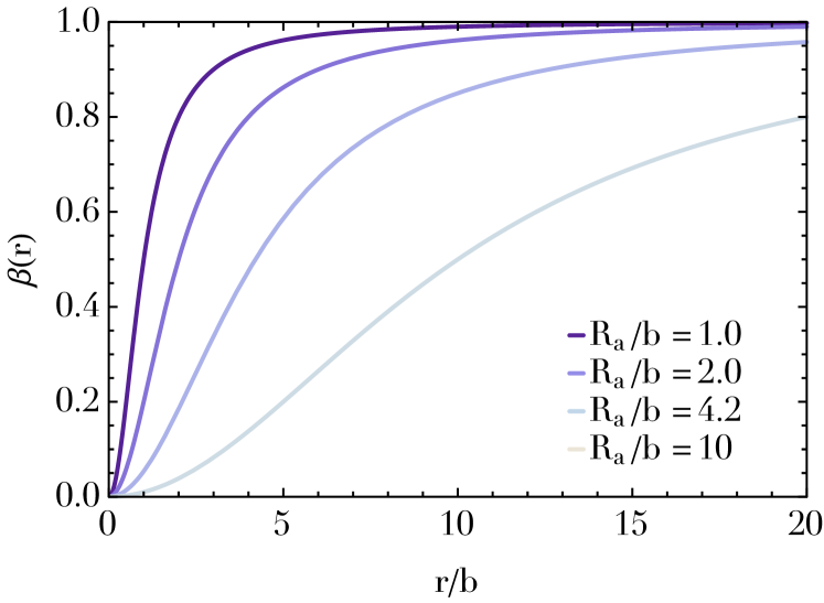
β(r)=11+Ra2/r2.𝛽𝑟11superscriptsubscript𝑅a2superscript𝑟2\beta(r)=\frac{1}{1+R_{\rm a}^{2}/r^{2}}. (64)

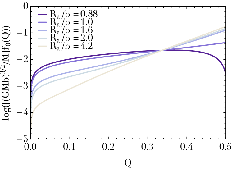
Hence Rasubscript𝑅aR_{{\rm a}} is called the ‘anisotropy radius’ and is the radius near which the velocity distribution transitions from isotropic at rRamuch-less-than𝑟subscript𝑅ar\ll R_{\rm a} to radially biased at rRamuch-greater-than𝑟subscript𝑅ar\gg R_{\rm a}. Fig. 1 shows the function f0(Q)subscript𝑓0𝑄f_{0}(Q) for several values of Rasubscript𝑅aR_{\rm a}, while Fig. 2 shows the corresponding runs of β(r)𝛽𝑟\beta(r).

Refer to caption

Figure 1: The Osipkov-Merritt DF f0(Q)subscript𝑓0𝑄f_{0}(Q) (equation (61)) as a function of Q𝑄Q. Note that for f0subscript𝑓0f_{0} to be well defined we require Ra>0.874bsubscript𝑅a0.874𝑏{R_{{\rm a}}>0.874b}.

Refer to caption

Figure 2: Anisotropy β1vt2/vr2𝛽1delimited-⟨⟩superscriptsubscript𝑣t2delimited-⟨⟩superscriptsubscript𝑣𝑟2{\beta\equiv 1-\langle v_{{\rm t}}^{2}\rangle/\langle v_{r}^{2}\rangle} as a function of radius r𝑟r for various anisotropy radii Rasubscript𝑅aR_{{\rm a}}.

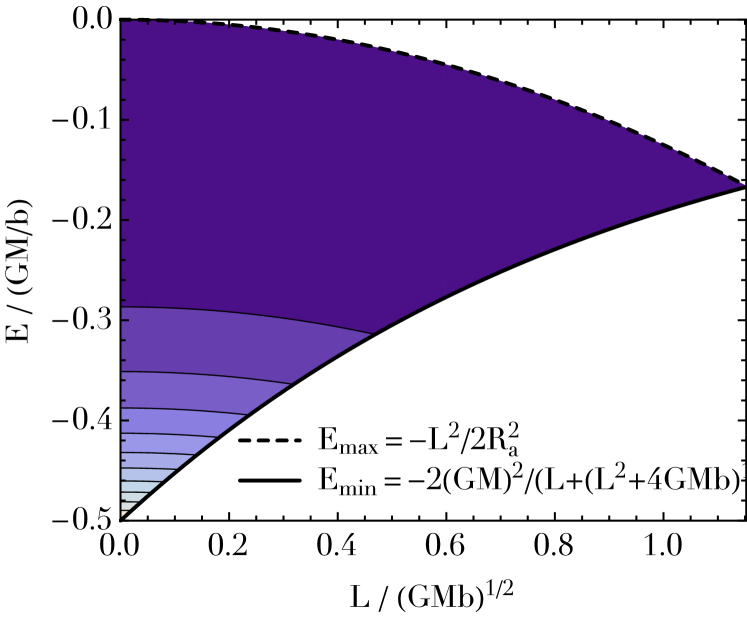
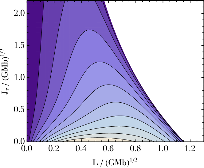
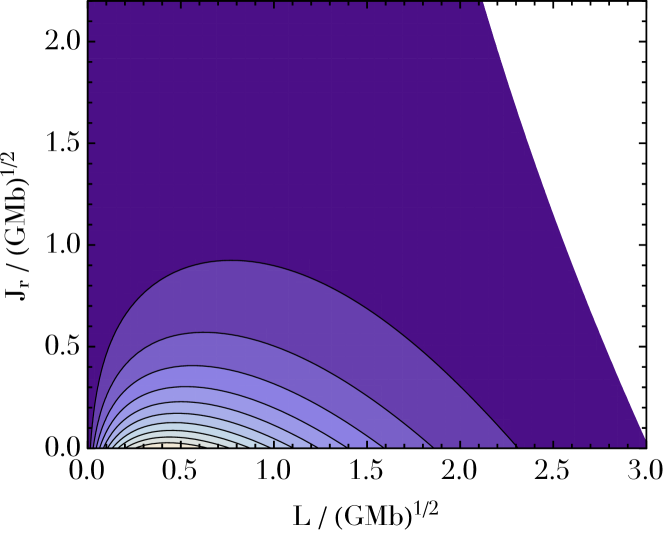
The model’s stars are confined to the part of the (E,L)𝐸𝐿(E,L) plane that is shaded in Figs. 3 and 4.

Refer to caption

Figure 3: Contours of f0(Q(E,L))subscript𝑓0𝑄𝐸𝐿{f_{0}(Q(E,L))} in the allowed part of (E,L)𝐸𝐿{(E,L)} space, for Ra=2bsubscript𝑅a2𝑏{R_{\rm a}=2b}. Contours are spaced linearly from the minimum (dark) to the maximum (light) values taken by f0(Q(E,L))subscript𝑓0𝑄𝐸𝐿{f_{0}(Q(E,L))}.

Refer to caption

Refer to caption

Figure 4: Contour plots of the two-dimensional DF f¯=2Lf0(Q)¯𝑓2𝐿subscript𝑓0𝑄\overline{f}=2Lf_{0}(Q) when Ra=2bsubscript𝑅a2𝑏R_{\rm a}=2b (above) and 10b10𝑏10b (below).

The lower boundary of this region is set by the requirement that E𝐸E be not smaller than the energy of a circular orbit at the given value of L𝐿L, which is

Emin=2(GM)2(L+L2+4GMb)2.subscript𝐸min2superscript𝐺𝑀2superscript𝐿superscript𝐿24𝐺𝑀𝑏2E_{\mathrm{min}}=-\frac{2(GM)^{2}}{\left(L+\sqrt{L^{2}+4GMb}\right)^{2}}. (65)

The upper boundary is simply the curve Q=0𝑄0Q=0. In addition, to have f00subscript𝑓00{f_{0}\geq 0} everywhere, we require Ra>0.874bsubscript𝑅a0.874𝑏{R_{{\rm a}}>0.874b}. By the Doremus-Feix-Baumann theorem (Binney & Tremaine, 2008, §5.5) the radial modes of a spherical model are all stable if f0/E<0subscript𝑓0𝐸0\partial f_{0}/\partial E<0 everywhere, and models with f0/L>0subscript𝑓0𝐿0\partial f_{0}/\partial L>0 tend to be unstable. We consider only models with Ra>0.97bsubscript𝑅a0.97𝑏{R_{{\rm a}}>0.97b} to ensure that f0/E<0subscript𝑓0𝐸0\partial f_{0}/\partial E<0 and f0/L<0subscript𝑓0𝐿0\partial f_{0}/\partial L<0 everywhere.

In significantly anisotropic models the boundary at Q=0𝑄0Q=0 generates large gradients in f𝑓f that are problematic numerically. Consequently, for models with Ra<10bsubscript𝑅a10𝑏R_{\rm a}<10b we have smoothed f𝑓f by multiplying it by e0.01/Qsuperscripte0.01𝑄\mathrm{e}^{-0.01/Q}.

We use the radial basis functions of Weinberg (1989) rescaled by a factor M/R𝑀𝑅M/\surd R, so they become

Un(r)superscriptsubscript𝑈𝑛𝑟\displaystyle U_{n}^{\ell}(r) =GMR4π2αn|j(αn)|j(αnr/R)absent𝐺𝑀𝑅4𝜋2subscript𝛼𝑛subscript𝑗subscript𝛼𝑛subscript𝑗subscript𝛼𝑛𝑟𝑅\displaystyle=-{GM\over R}{4\pi\surd 2\over\alpha_{\ell n}|j_{\ell}(\alpha_{\ell n})|}j_{\ell}(\alpha_{\ell n}r/R) (66)
Dn(r)superscriptsubscript𝐷𝑛𝑟\displaystyle D_{n}^{\ell}(r) =MR3αn2|j(αn)|j(αnr/R),absent𝑀superscript𝑅3subscript𝛼𝑛2subscript𝑗subscript𝛼𝑛subscript𝑗subscript𝛼𝑛𝑟𝑅\displaystyle={M\over R^{3}}{\alpha_{\ell n}\surd 2\over|j_{\ell}(\alpha_{\ell n})|}j_{\ell}(\alpha_{\ell n}r/R), (67)

where the density is assumed to vanish beyond the truncation radius R𝑅R, jsubscript𝑗j_{\ell} is a spherical Bessel function of the first kind and αnsubscript𝛼𝑛\alpha_{\ell n} is the n𝑛nth zero of jsubscript𝑗j_{\ell}. For these basis functions the normalising constant in equation (19) is

=4πGM2R.4𝜋𝐺superscript𝑀2𝑅{\cal E}=4\pi{GM^{2}\over R}. (68)

5.1 Calculation of the response matrix

To ensure that our code is applicable to any spherical model and not just isochrone models, we use as coordinates for orbit space the radii rpsubscript𝑟pr_{\rm p} and rasubscript𝑟ar_{\rm a} of peri- and apo-centre rather than Jrsubscript𝐽𝑟J_{r} and L𝐿L. These radii are the roots of the equation

EΦ(r)L22r2=0.𝐸Φ𝑟superscript𝐿22superscript𝑟20E-\Phi(r)-\frac{L^{2}}{2r^{2}}=0. (69)

Hence, given rpsubscript𝑟pr_{\rm p} and rasubscript𝑟ar_{\rm a} it follows easily that

E=ra2Φ(ra)rp2Φ(rp)ra2rp2;L=2[Φ(ra)Φ(rp)]rp2ra2.formulae-sequence𝐸superscriptsubscript𝑟a2Φsubscript𝑟asuperscriptsubscript𝑟p2Φsubscript𝑟psuperscriptsubscript𝑟a2superscriptsubscript𝑟p2𝐿2delimited-[]Φsubscript𝑟aΦsubscript𝑟psuperscriptsubscript𝑟p2superscriptsubscript𝑟a2E=\frac{r_{{\rm a}}^{2}\Phi(r_{{\rm a}})-r_{{\rm p}}^{2}\Phi(r_{{\rm p}})}{r_{{\rm a}}^{2}-r_{{\rm p}}^{2}};\,\,\,\,\,\,\,\,\,\,L=\sqrt{\frac{2[\Phi(r_{{\rm a}})-\Phi(r_{{\rm p}})]}{r_{{\rm p}}^{-2}-r_{{\rm a}}^{-2}}}. (70)

Putting H=E𝐻𝐸H=E in the Hamiltonian (60) we recover Jr(rp,ra)subscript𝐽𝑟subscript𝑟psubscript𝑟aJ_{r}(r_{\rm p},r_{\rm a}). Integrals over d2𝐉~superscriptd2~𝐉{\rm d}^{2}\widetilde{\bf J} can be expressed as integrals over (rp,ra)subscript𝑟psubscript𝑟a(r_{\rm p},r_{\rm a}) using the Jacobian

(Jr,L)(rp,ra)=(Jr,L)(E,L)(E,L)(rp,ra)=1Ωr(E,L)(rp,ra).subscript𝐽𝑟𝐿subscript𝑟psubscript𝑟asubscript𝐽𝑟𝐿𝐸𝐿𝐸𝐿subscript𝑟psubscript𝑟a1subscriptΩ𝑟𝐸𝐿subscript𝑟psubscript𝑟a\frac{\partial(J_{r},L)}{\partial(r_{\rm p},r_{\rm a})}=\frac{\partial(J_{r},L)}{\partial(E,L)}\frac{\partial(E,L)}{\partial(r_{\rm p},r_{\rm a})}={1\over\Omega_{r}}\frac{\partial(E,L)}{\partial(r_{\rm p},r_{\rm a})}. (71)

Since f0=f0(Q(E,L))subscript𝑓0subscript𝑓0𝑄𝐸𝐿{f_{0}=f_{0}\left(Q(E,L)\right)}, we have

𝐧~f0𝐉~=bGMdf0dQ[n1Ωr+n2(Ωϑ+LRa2)].~𝐧subscript𝑓0~𝐉𝑏𝐺𝑀dsubscript𝑓0d𝑄delimited-[]subscript𝑛1subscriptΩ𝑟subscript𝑛2subscriptΩitalic-ϑ𝐿superscriptsubscript𝑅a2\widetilde{\bf n}\cdot{\partial f_{0}\over\partial\widetilde{\bf J}}=-\frac{b}{GM}\frac{\mathrm{d}f_{0}}{\mathrm{d}Q}\left[n_{1}\Omega_{r}+n_{2}\left(\Omega_{\vartheta}+\frac{L}{R_{{\rm a}}^{2}}\right)\right].

To perform the integration numerically over the (rp,ra)subscript𝑟psubscript𝑟a(r_{\rm p},r_{\rm a}) plane implied by equation (4), we divide the plane into regions labelled by i𝑖i. The i𝑖ith region is centred at (rpi,rai)superscriptsubscript𝑟p𝑖superscriptsubscript𝑟a𝑖{(r_{{\rm p}}^{i},r_{{\rm a}}^{i})} and covers the square rp[rpiΔr/2,rpi+Δr/2],ra[raiΔr/2,rai+Δr/2]formulae-sequencesubscript𝑟psuperscriptsubscript𝑟p𝑖Δ𝑟2superscriptsubscript𝑟p𝑖Δ𝑟2subscript𝑟asuperscriptsubscript𝑟a𝑖Δ𝑟2superscriptsubscript𝑟a𝑖Δ𝑟2{r_{{\rm p}}\in[r_{{\rm p}}^{i}-\Delta r/2,r_{{\rm p}}^{i}+\Delta r/2],\,\,\,r_{{\rm a}}\in[r_{{\rm a}}^{i}-\Delta r/2,r_{{\rm a}}^{i}+\Delta r/2]}. Then in each region we separately Taylor expand the frequency 𝐧~~𝛀ω~𝐧~absent𝛀𝜔\widetilde{\bf n}\cdot\widetilde{}\mbox{\boldmath$\Omega$}-\omega that appears as the denominator in equation (4) and its numerator. The ratio of Taylor expansions is then analytically integrated through the region. The numerical steps involved are exactly those that have been detailed extensively in Fouvry et al. (2015) so we will not repeat the recipe here.

The most computationally expensive part of this procedure is the calculation from equation (38) of the matrix elements W𝑊W at each point on the (rp,ra)subscript𝑟psubscript𝑟a{(r_{{\rm p}},r_{{\rm a}})} grid. It is important that we use a large, dense grid, as the biggest contributions to 𝐧~f0/𝐉~~𝐧subscript𝑓0~𝐉\widetilde{\bf n}\cdot\partial f_{0}/\partial\widetilde{\bf J} come from the edge of the model, where |df0/dQ|dsubscript𝑓0d𝑄|\mathrm{d}f_{0}/\mathrm{d}Q| is largest. However, for small values of Rasubscript𝑅aR_{\rm a} the requirement Q>0𝑄0Q>0 usefully restricts the portion of the (rp,ra)subscript𝑟psubscript𝑟a(r_{\rm p},r_{\rm a}) grid within which the matrix elements of W𝑊W need to be computed (Fig. 3). For this reason fluxes are more easily computed for models with small values of Rasubscript𝑅aR_{\rm a} than large ones.

5.2 Recovering unstable modes

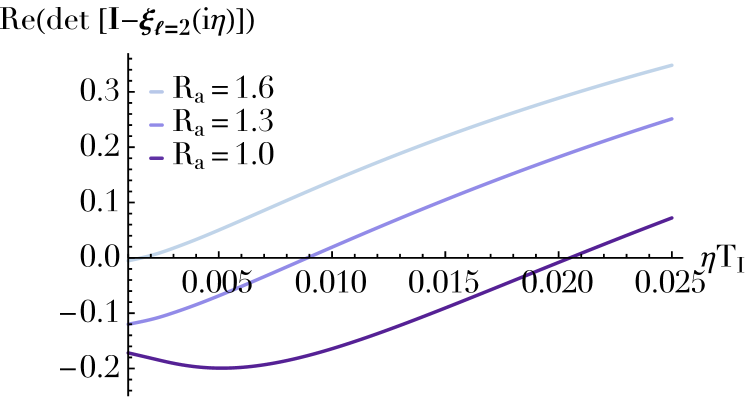
To demonstrate that our evaluation of the response matrix 𝐌(ω)𝐌𝜔\mathbf{M}(\omega) is correct, we recover the known unstable modes of our system. For a spherical system the perturbations can be conveniently decomposed into spherical harmonics Ymsuperscriptsubscript𝑌𝑚Y_{\ell}^{m}, and we can consider each harmonic \ell separately. Modes correspond to frequencies ω=ω0+iη𝜔subscript𝜔0i𝜂{\omega=\omega_{0}+\mathrm{i}\eta} with η>0𝜂0\eta>0 for which the matrix =𝐈𝐌(ω)𝐈𝐌𝜔{\mathchoice{\hbox{{\gkvecten\char 15\relax}}}{\hbox{{\gkvecten\char 15\relax}}}{\hbox{{\gkvecseven\char 15\relax}}}{\hbox{{\gkvecseven\char 15\relax}}}}={\bf I}-{\bf M}(\omega) has a zero eigenvalue; in other words, we seek ω𝜔\omega such that

det=0.0\det{\mathchoice{\hbox{{\gkvecten\char 15\relax}}}{\hbox{{\gkvecten\char 15\relax}}}{\hbox{{\gkvecseven\char 15\relax}}}{\hbox{{\gkvecseven\char 15\relax}}}}=0. (72)

The mode has frequency ω0subscript𝜔0\omega_{0} and growth rate η𝜂\eta. Since from equation (42)

ϵpq=δqδmpmq[δnpnqξnpnq(ω)].subscriptitalic-ϵ𝑝𝑞superscriptsubscript𝛿superscript𝑞superscriptsubscript𝛿superscript𝑚𝑝superscript𝑚𝑞delimited-[]superscriptsubscript𝛿superscript𝑛𝑝superscript𝑛𝑞subscript𝜉superscript𝑛𝑝superscript𝑛𝑞𝜔\epsilon_{pq}=\delta_{\ell}^{\ell^{q}}\delta_{m^{p}}^{m^{q}}[\delta_{n^{p}}^{n^{q}}-\xi_{\ell n^{p}n^{q}}(\omega)]. (73)

for each fixed \ell we need to compute the determinant of the matrix δnpnq(¸)npnqsuperscriptsubscript𝛿superscript𝑛𝑝superscript𝑛𝑞subscriptsubscript¸superscript𝑛𝑝superscript𝑛𝑞{\delta_{n^{p}}^{n^{q}}-({\mathchoice{\hbox{{\gkvecten\char 24\relax}}}{\hbox{{\gkvecten\char 24\relax}}}{\hbox{{\gkvecseven\char 24\relax}}}{\hbox{{\gkvecseven\char 24\relax}}}}_{\ell})_{n^{p}n^{q}}}.

Saha (1991) used the Osipkov-Merritt DF (61) to study the radial-orbit instability in anisotropic isochrone models. He found that a mode with =22{\ell=2} becomes unstable when Rasubscript𝑅aR_{\rm a} falls below 4bsimilar-toabsent4𝑏\sim 4b. In terms of the natural unit of time TI=b3/GMsubscript𝑇Isuperscript𝑏3𝐺𝑀T_{\mathrm{I}}=\sqrt{b^{3}/GM}, growth rates η𝜂\eta are very small (η0.001/TImuch-less-than𝜂0.001subscript𝑇I{\eta\ll 0.001/T_{\rm I}}) when the mode first becomes unstable but grow towards η0.025/TI𝜂0.025subscript𝑇I{\eta\approx 0.025/T_{\rm I}} as Rabsubscript𝑅a𝑏R_{{\rm a}}\to b.444Saha’s Figure 2(b) shows the growth rates η𝜂\eta for various anisotropies β𝛽\beta. To convert between Saha’s β𝛽\beta and Rasubscript𝑅aR_{\rm a}, use his Figure 1.

The calculations in Saha (1991) used 101010 radial basis functions Unsuperscriptsubscript𝑈𝑛U_{n}^{\ell} from a different family from that used here, and focused on =22\ell=2. Since in a spherical system the growth rate must be independent of the azimuthal part of the spherical harmonics, Saha set m=0𝑚0m=0. The unstable mode has vanishing pattern speed, so in searching for it Saha set ω0=0subscript𝜔00\omega_{0}=0. We follow all of these conventions. In our standard computation the truncation radius of the basis functions is R=20b𝑅20𝑏R=20b, and the grid in {(rpi,rai)}subscriptsuperscript𝑟𝑖psubscriptsuperscript𝑟𝑖a{\{(r^{i}_{{\rm p}},r^{i}_{{\rm a}})\}} covers the range ri[0.15b,19.85b]superscript𝑟𝑖0.15𝑏19.85𝑏{r^{i}\in[0.15b,19.85b]} with grid spacing Δr=0.1bΔ𝑟0.1𝑏{\Delta r=0.1b}. Finally, the maximum index n1subscript𝑛1n_{1} in the sum of equation (4) is n1=nmax=4subscript𝑛1superscript𝑛max4n_{1}=n^{\mathrm{max}}=4. The justification for this choice is that the isochrone’s frequencies satisfy

Ω2Ω1=12(1+J2J22+4GMb),subscriptΩ2subscriptΩ1121subscript𝐽2superscriptsubscript𝐽224𝐺𝑀𝑏{\Omega_{2}\over\Omega_{1}}={\textstyle{1\over 2}}\left(1+{J_{2}\over\sqrt{J_{2}^{2}+4GMb}}\right)\,, (74)

so orbits with J22GMbmuch-less-thansubscript𝐽22𝐺𝑀𝑏J_{2}\ll 2\sqrt{GMb} satisfy 2Ω2Ω102subscriptΩ2subscriptΩ102\Omega_{2}-\Omega_{1}\approx 0. Consequently, we expect equation (4) to be dominated by the term with (n1,n2)=±(1,2)subscript𝑛1subscript𝑛2plus-or-minus12(n_{1},n_{2})=\pm(1,-2).

Since η𝜂\eta is very small and all other contributions to the response matrix are real, the imaginary part of det[𝐈¸=2(iη)]delimited-[]𝐈subscript¸2i𝜂{\det[\mathbf{I}-{\mathchoice{\hbox{{\gkvecten\char 24\relax}}}{\hbox{{\gkvecten\char 24\relax}}}{\hbox{{\gkvecseven\char 24\relax}}}{\hbox{{\gkvecseven\char 24\relax}}}}_{\ell=2}(\mathrm{i}\eta)]} is negligible. Hence to locate the unstable modes, we need only plot Re(det[𝐈¸=2(iη)])Redelimited-[]𝐈subscript¸2i𝜂{\mathrm{Re}\left(\det[\mathbf{I}-{\mathchoice{\hbox{{\gkvecten\char 24\relax}}}{\hbox{{\gkvecten\char 24\relax}}}{\hbox{{\gkvecseven\char 24\relax}}}{\hbox{{\gkvecseven\char 24\relax}}}}_{\ell=2}(\mathrm{i}\eta)]\right)} for various values of the growth rate η𝜂\eta, and pick out the η𝜂\eta for which Re(det[𝐈¸=2(iη)])=0Redelimited-[]𝐈subscript¸2i𝜂0{\mathrm{Re}\left(\det[\mathbf{I}-{\mathchoice{\hbox{{\gkvecten\char 24\relax}}}{\hbox{{\gkvecten\char 24\relax}}}{\hbox{{\gkvecseven\char 24\relax}}}{\hbox{{\gkvecseven\char 24\relax}}}}_{\ell=2}(\mathrm{i}\eta)]\right)=0}. Fig. 5 shows Re(det[𝐈¸=2(iη)])Redelimited-[]𝐈subscript¸2i𝜂\mathrm{Re}\left(\det[\mathbf{I}-{\mathchoice{\hbox{{\gkvecten\char 24\relax}}}{\hbox{{\gkvecten\char 24\relax}}}{\hbox{{\gkvecseven\char 24\relax}}}{\hbox{{\gkvecseven\char 24\relax}}}}_{\ell=2}(\mathrm{i}\eta)]\right) as a function of η𝜂\eta for three values of Rasubscript𝑅aR_{\rm a}.

Refer to caption

Figure 5: Plot of Re(det[𝐈¸=2(0+iη)])Redelimited-[]𝐈subscript¸20i𝜂{\mathrm{Re}\left(\det[\mathbf{I}-{\mathchoice{\hbox{{\gkvecten\char 24\relax}}}{\hbox{{\gkvecten\char 24\relax}}}{\hbox{{\gkvecseven\char 24\relax}}}{\hbox{{\gkvecseven\char 24\relax}}}}_{\ell=2}(0+\mathrm{i}\eta)]\right)} in units of TIsubscript𝑇IT_{\rm I} as a function of the growth rate η𝜂\eta for Ra/b=1.0,1.3,1.6subscript𝑅a𝑏1.01.31.6{R_{\rm a}/b=1.0,1.3,1.6} (from bottom to top). Crossing the η𝜂\eta axis indicates the existence of the radial-orbit instability.

Each curve crosses the x𝑥x axis, so all these models are subject to the radial-orbit instability. However, the model with Ra=1.6bsubscript𝑅a1.6𝑏R_{\rm a}=1.6b only just manages to cross the x𝑥x axis, suggesting that the limiting value for instability, Ra,maxsubscript𝑅amaxR_{\rm a,max} lies close to 1.6b1.6𝑏1.6b. This conclusion is consistent with the conclusion of May & Binney (1986) that Ra,max1.67bsimilar-to-or-equalssubscript𝑅amax1.67𝑏R_{\rm a,max}\simeq 1.67b. The top row of Table 1 gives our growth rates for these four models plus indications that models with Ra/b2subscript𝑅a𝑏2R_{\rm a}/b\geq 2 are stable.

Table 1: Growth rates for the radial-orbit instability in the isochrone model. We compare values from our standard computation with values from Saha (1991). The notation ×ysubscript𝑦\times_{y} means that we could not recover an unstable mode, and that the value of Re(det[𝐈¸=2(iη)])Redelimited-[]𝐈subscript¸2i𝜂{\mathrm{Re}\left(\det[\mathbf{I}-{\mathchoice{\hbox{{\gkvecten\char 24\relax}}}{\hbox{{\gkvecten\char 24\relax}}}{\hbox{{\gkvecseven\char 24\relax}}}{\hbox{{\gkvecseven\char 24\relax}}}}_{\ell=2}(\mathrm{i}\eta)]\right)} at η=0𝜂0\eta=0 was y𝑦y.
Ra/bsubscript𝑅a𝑏R_{\rm a}/b 1.0 1.3 1.6 2.0 3.0 4.2
Our ηTI𝜂subscript𝑇I\eta T_{\rm I} 0.021 0.009 0.002 ×0.20subscript0.20\times_{0.20} ×0.43subscript0.43\times_{0.43} ×0.53subscript0.53\times_{0.53}
Saha linear ηTI𝜂subscript𝑇I\eta T_{\rm I} 0.024 0.009 0.004 <0.001absent0.001<0.001 0.001much-less-thanabsent0.001\ll 0.001 0.001very-much-less-thanabsent0.001\lll 0.001
Saha N-body ηTI𝜂subscript𝑇I\eta T_{\rm I} 0.029 0.015 0.010

The second and third rows of Table 1 give corresponding results from Saha (1991). Our growth rates tend to be slightly smaller than the rates Saha obtained from linear theory, and significantly smaller than the rates Saha inferred from N-body simulations, especially for the marginally unstable model.

Linear theory enables us to predict the shape (but not the amplitude) of the perturbation to the potential associated with an unstable mode. Indeed, with η𝜂\eta the growth rate of the unstable mode, ¸=2(iη)subscript¸2i𝜂{\mathchoice{\hbox{{\gkvecten\char 24\relax}}}{\hbox{{\gkvecten\char 24\relax}}}{\hbox{{\gkvecseven\char 24\relax}}}{\hbox{{\gkvecseven\char 24\relax}}}}_{\ell=2}(\mathrm{i}\eta) is an Hermitian matrix (to see this, take the Hermitian conjugate of equation (4) and use Wn𝐧~=Wn𝐧~subscriptsuperscript𝑊~𝐧𝑛subscriptsuperscript𝑊~𝐧𝑛W^{\widetilde{\mathbf{n}}}_{\ell n}=W^{-\widetilde{\mathbf{n}}}_{\ell n}). It has an eigenvector 𝐗𝐗{\bf X} with eigenvalue unity, and the perturbation to the potential is

Φ1(𝐱)subscriptΦ1𝐱\displaystyle\Phi_{1}({\bf x}) Re[n=1nmaxXnΦ(n,2,0)(𝐱)]proportional-toabsentRedelimited-[]superscriptsubscript𝑛1superscript𝑛maxsuperscript𝑋𝑛superscriptΦ𝑛20𝐱\displaystyle\propto\mathrm{Re}\left[\sum_{n=1}^{n^{\rm max}}X^{n}\Phi^{(n,2,0)}({\bf x})\right] (75)
=[n=1nmaxXnj2(α2nr/R)α2n|j2(α2n)|]P2(cosθ).absentdelimited-[]superscriptsubscript𝑛1superscript𝑛maxsuperscript𝑋𝑛subscript𝑗2subscript𝛼2𝑛𝑟𝑅subscript𝛼2𝑛subscript𝑗2subscript𝛼2𝑛subscript𝑃2𝜃\displaystyle=\left[\sum_{n=1}^{n^{\rm max}}X^{n}{j_{2}(\alpha_{2n}r/R)\over\alpha_{2n}\left|j_{2}(\alpha_{2n})\right|}\right]P_{2}(\cos\theta). (76)

The purple line in Fig. 6 shows Φ1subscriptΦ1\Phi_{1} when Ra=bsubscript𝑅a𝑏R_{\rm a}=b, while the black curve reproduces the corresponding plot from Saha (1991).
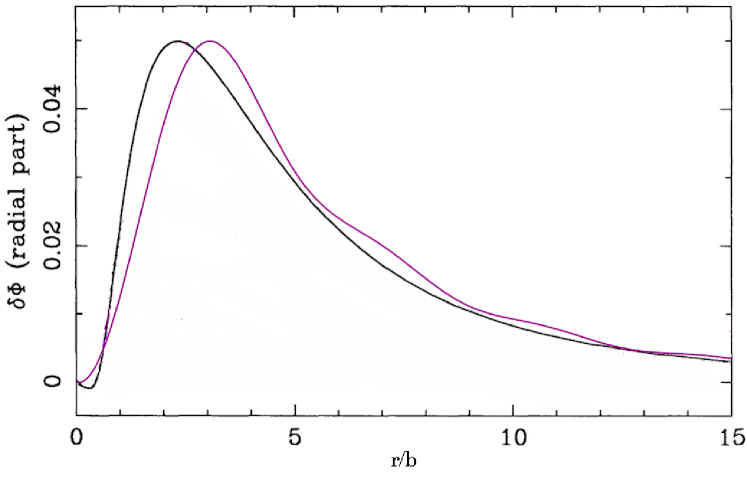
Refer to caption

Figure 6: The radial part of our Φ1subscriptΦ1\Phi_{1} (what Saha calls δΦ𝛿Φ\delta\Phi) in purple, superimposed on Saha’s version of the same mode (black), for the unstable =22{\ell=2} mode in the model with Ra=bsubscript𝑅a𝑏{R_{\mathrm{a}}=b}. The normalisation of the vertical axis is arbitrary. (Graphics edited from Saha (1991)).

Overall the agreement is good.

5.2.1 Convergence study

Table 2 shows how the recovered growth rates of the radial-orbit instability (=22\ell=2) are affected by changing the four key parameters of the computation.

Table 2: Growth rates for the radial-orbit instability in the isochrone model computed for various values of the parameters that control the precision of the calculations. The tabulated values are of ηTI𝜂subscript𝑇I\eta T_{\rm I} and the values in bold are from our standard computation. The notation ×ysubscript𝑦\times_{y} means that we could not recover an unstable mode, and that the value of Re(det[𝐈¸=2(iη)])Redelimited-[]𝐈subscript¸2i𝜂{\mathrm{Re}\left(\det[\mathbf{I}-{\mathchoice{\hbox{{\gkvecten\char 24\relax}}}{\hbox{{\gkvecten\char 24\relax}}}{\hbox{{\gkvecseven\char 24\relax}}}{\hbox{{\gkvecseven\char 24\relax}}}}_{\ell=2}(\mathrm{i}\eta)]\right)} at η=0𝜂0\eta=0 was y𝑦y.
Anisotropy radius Ra/bsubscript𝑅a𝑏R_{\mathrm{a}}/b 1.01.01.0 1.31.31.3 1.61.61.6 2.02.02.0 3.03.03.0 4.24.24.2
Δr/b=0.05Δ𝑟𝑏0.05\Delta r/b=0.05 0.02100.02100.0210 0.01110.01110.0111 ×0.01subscript0.01\times_{0.01} ×0.19subscript0.19\times_{0.19} ×0.43subscript0.43\times_{0.43} ×0.53subscript0.53\times_{0.53}
Δr/b=0.07Δ𝑟𝑏0.07\Delta r/b=0.07 0.02200.02200.0220 0.01000.01000.0100 ×0.02subscript0.02\times_{0.02} ×0.19subscript0.19\times_{0.19} ×0.43subscript0.43\times_{0.43} ×0.53subscript0.53\times_{0.53}
Δr/b=0.1Δ𝑟𝑏0.1\Delta r/b={\bf 0.1} 0.02050.0205{\bf 0.0205} 0.00890.0089{\bf 0.0089} 0.00160.0016{\bf 0.0016} ×0.20subscript0.20\times_{0.20} ×0.43subscript0.43\times_{0.43} ×0.53subscript0.53\times_{0.53}
Δr/b=0.15Δ𝑟𝑏0.15\Delta r/b=0.15 0.02000.02000.0200 0.00810.00810.0081 0.00680.00680.0068 ×0.17subscript0.17\times_{0.17} ×0.44subscript0.44\times_{0.44} ×0.54subscript0.54\times_{0.54}
Δr/b=0.2Δ𝑟𝑏0.2\Delta r/b=0.2 0.02450.02450.0245 0.00970.00970.0097 0.00570.00570.0057 ×0.22subscript0.22\times_{0.22} ×0.44subscript0.44\times_{0.44} ×0.54subscript0.54\times_{0.54}
Δr/b=0.3Δ𝑟𝑏0.3\Delta r/b=0.3 0.02220.02220.0222 0.00850.00850.0085 ×0.03subscript0.03\times_{0.03} ×0.21subscript0.21\times_{0.21} ×0.45subscript0.45\times_{0.45} ×0.55subscript0.55\times_{0.55}
R/b=10𝑅𝑏10R/b=10 0.02030.02030.0203 ×0.01subscript0.01\times_{0.01} ×0.15subscript0.15\times_{0.15} ×0.27subscript0.27\times_{0.27} ×0.39subscript0.39\times_{0.39} ×0.45subscript0.45\times_{0.45}
R/b=16𝑅𝑏16R/b=16 0.02160.02160.0216 0.00840.00840.0084 0.00160.00160.0016 ×0.22subscript0.22\times_{0.22} ×0.41subscript0.41\times_{0.41} ×0.50subscript0.50\times_{0.50}
R/b=𝟐𝟎𝑅𝑏20R/b={\bf 20} 0.02050.0205{\bf 0.0205} 0.00890.0089{\bf 0.0089} 0.00160.0016{\bf 0.0016} ×0.20subscript0.20\times_{0.20} ×0.43subscript0.43\times_{0.43} ×0.53subscript0.53\times_{0.53}
R/b=25𝑅𝑏25R/b=25 0.01800.01800.0180 0.00810.00810.0081 0.00260.00260.0026 ×0.17subscript0.17\times_{0.17} ×0.43subscript0.43\times_{0.43} ×0.56subscript0.56\times_{0.56}
n1max=1superscriptsubscript𝑛1max1n_{1}^{\mathrm{max}}=1 0.02080.02080.0208 0.00890.00890.0089 0.00140.00140.0014 ×0.19subscript0.19\times_{0.19} ×0.43subscript0.43\times_{0.43} ×0.54subscript0.54\times_{0.54}
n1max=2superscriptsubscript𝑛1max2n_{1}^{\mathrm{max}}=2 0.02040.02040.0204 0.00880.00880.0088 0.00150.00150.0015 ×0.19subscript0.19\times_{0.19} ×0.43subscript0.43\times_{0.43} ×0.54subscript0.54\times_{0.54}
n1max=𝟒superscriptsubscript𝑛1max4n_{1}^{\mathrm{max}}={\bf 4} 0.02050.0205{\bf 0.0205} 0.00890.0089{\bf 0.0089} 0.00160.0016{\bf 0.0016} ×0.20subscript0.20\times_{0.20} ×0.43subscript0.43\times_{0.43} ×0.53subscript0.53\times_{0.53}
n1max=6superscriptsubscript𝑛1max6n_{1}^{\mathrm{max}}=6 0.02050.02050.0205 0.00890.00890.0089 0.00170.00170.0017 ×0.19subscript0.19\times_{0.19} ×0.42subscript0.42\times_{0.42} ×0.53subscript0.53\times_{0.53}
n1max=8superscriptsubscript𝑛1max8n_{1}^{\mathrm{max}}=8 0.02060.02060.0206 0.00900.00900.0090 0.00170.00170.0017 ×0.19subscript0.19\times_{0.19} ×0.42subscript0.42\times_{0.42} ×0.52subscript0.52\times_{0.52}
nmax=8superscript𝑛max8n^{\mathrm{max}}=8 0.01820.01820.0182 0.00790.00790.0079 0.00010.00010.0001 ×0.22subscript0.22\times_{0.22} ×0.47subscript0.47\times_{0.47} ×0.58subscript0.58\times_{0.58}
nmax=𝟏𝟎superscript𝑛max10n^{\mathrm{max}}={\bf 10} 0.02050.0205{\bf 0.0205} 0.00890.0089{\bf 0.0089} 0.00160.0016{\bf 0.0016} ×0.20subscript0.20\times_{0.20} ×0.43subscript0.43\times_{0.43} ×0.53subscript0.53\times_{0.53}
nmax=13superscript𝑛max13n^{\mathrm{max}}=13 0.02200.02200.0220 0.00960.00960.0096 0.00200.00200.0020 ×0.17subscript0.17\times_{0.17} ×0.38subscript0.38\times_{0.38} ×0.48subscript0.48\times_{0.48}
nmax=16superscript𝑛max16n^{\mathrm{max}}=16 0.02240.02240.0224 0.00980.00980.0098 0.00230.00230.0023 ×0.15subscript0.15\times_{0.15} ×0.34subscript0.34\times_{0.34} ×0.43subscript0.43\times_{0.43}

These are (i) the spacing ΔrΔ𝑟\Delta r of the grid in rpsubscript𝑟pr_{\rm p} and rasubscript𝑟ar_{\rm a}; (ii) the truncation radius R𝑅R of the basis functions (which also sets the upper limit on values of rpsubscript𝑟pr_{\rm p} and rasubscript𝑟ar_{\rm a}); (iii) the maximum included value of the quantum number n1subscript𝑛1n_{1} associated with Jrsubscript𝐽𝑟J_{r}; (iv) the number nmaxsuperscript𝑛maxn^{\rm max} of basis functions summed over (equation (75)). The results for the significantly unstable models, Ra=1subscript𝑅a1R_{\rm a}=1 and 1.3, show gratifyingly little sensitivity to these parameters. The most significant fact is that dropping R𝑅R to 10b10𝑏10b killed the instability in the model with Ra=1.3bsubscript𝑅a1.3𝑏R_{\rm a}=1.3b. The results for the marginally unstable model Ra=1.6bsubscript𝑅a1.6𝑏R_{\rm a}=1.6b do change significantly with the values of parameters, but clear trends are not evident. It is notable that experimenting with different parameter values does not change the conclusion that the model with Ra=2bsubscript𝑅a2𝑏R_{\rm a}=2b is stable. No modification produced a curve of Re(det[𝐈¸=2(iη)])Redelimited-[]𝐈subscript¸2i𝜂\mathrm{Re}\left(\det[\mathbf{I}-{\mathchoice{\hbox{{\gkvecten\char 24\relax}}}{\hbox{{\gkvecten\char 24\relax}}}{\hbox{{\gkvecseven\char 24\relax}}}{\hbox{{\gkvecseven\char 24\relax}}}}_{\ell=2}(\mathrm{i}\eta)]\right) that differed significantly from those plotted in Fig. 5.

Tables 1 and 2 in conjunction with Fig. 6 give us confidence that the response matrix is being calculated correctly.

5.3 Calculation of the Balescu–Lenard flux

The magnitude of the diffusive flux 𝐅¯¯𝐅\overline{\bf F} is a direct measure of a system’s relaxation rate: as the relaxation timescale tends to infinity, the diffusive flux tends to zero. Hence we now compute from equations (57) and (4) the diffusive flux in the LJr𝐿subscript𝐽𝑟LJ_{r} plane. In Section 6 we will compare this flux with that predicted by classical theory.

The sum over \ell in equation (4) can be pulled out front, so we obtain the flux

𝐅¯=𝐅¯,¯𝐅subscriptsubscript¯𝐅\overline{{\bf F}}=\sum_{\ell}\overline{{\bf F}}_{\ell}, (77)

as a sum of contributions from each multipole. For given 𝐧~,𝐧~~𝐧superscript~𝐧\widetilde{\bf n},\widetilde{\bf n}^{\prime}, the integrand on the right of equation (4) can be straightforwardly computed from equations (4) and (43), so the only challenge is the evaluation of the integral over 𝐉~superscript~𝐉\widetilde{\bf J}^{\prime}, which has the general form

d2𝐉~g(𝐉~)δ(h(𝐉~)).superscriptd2superscript~𝐉𝑔superscript~𝐉𝛿superscript~𝐉\int{\rm d}^{2}\widetilde{\bf J}^{\prime}\,g(\widetilde{\bf J}^{\prime})\,\delta\big{(}h(\widetilde{\bf J}^{\prime})\big{)}. (78)

Following Fouvry et al. (2015), this may be written

Cdσ(𝐉~)g(𝐉~)|h(𝐉~)|,subscript𝐶differential-d𝜎superscript~𝐉𝑔superscript~𝐉superscript~𝐉\int_{C}\mathrm{d}\sigma(\widetilde{\bf J}^{\prime})\,\frac{g(\widetilde{\bf J}^{\prime})}{\left|\nabla h(\widetilde{\bf J}^{\prime})\right|}, (79)

where C𝐶C is the curve along which the resonant condition 0=h(𝐉)=𝐧~~𝛀𝐧~~𝛀0superscript𝐉superscript~𝐧~absentsuperscript𝛀~𝐧~absent𝛀0=h({\bf J}^{\prime})=\widetilde{\bf n}^{\prime}\cdot\widetilde{}\mbox{\boldmath$\Omega$}^{\prime}-\widetilde{\bf n}\cdot\widetilde{}\mbox{\boldmath$\Omega$} is satisfied, and dσ(𝐉~)d𝜎superscript~𝐉{\rm d}\sigma(\widetilde{\bf J}^{\prime}) is the line element on C𝐶C. Details of the evaluation of the resulting line integral can be found in Fouvry et al. (2015).

5.3.1 Wavevectors to consider

To evaluate the BL flux we have to perform a sum over all possible ‘pairs’ (𝐧~,𝐧~)~𝐧superscript~𝐧(\widetilde{\bf n},\widetilde{\bf n}^{\prime}) of two-dimensional vectors with integer components. By a slight abuse of language, we shall refer to objects like 𝐧~~𝐧\widetilde{\bf n} as ‘wavevectors’. In principle there are infinitely many of these wavevector pairs, but some of them do not contribute to the flux. To eliminate pairs which do not contribute we first note that for each value of \ell we can restrict ourselves to pairs for which the quantity Λ𝐧~𝐧~superscriptsubscriptΛ~𝐧superscript~𝐧\Lambda_{{\widetilde{\bf n}\widetilde{\bf n}^{\prime}}}^{\ell} defined by equation (4) is non-zero. From the appearance in this equation of n~2subscript~𝑛2\widetilde{n}_{2} and n~2superscriptsubscript~𝑛2\widetilde{n}_{2}^{\prime} as superscripts of spherical harmonics it is clear that the sum can be restricted to |n~2|subscript~𝑛2|\widetilde{n}_{2}|\leq\ell and |n~2|superscriptsubscript~𝑛2|\widetilde{n}_{2}^{\prime}|\leq\ell. Moreover, the spherical harmonics vanish unless n~2subscript~𝑛2\ell-\widetilde{n}_{2} and n~2superscriptsubscript~𝑛2\ell-\widetilde{n}_{2}^{\prime} are even. Hence the values to be included are

=0:n~2=0=2:n~2=±2,0=1:n~2=±1=3:n~2=±3,±1=4:n~2=0,±2,±4,matrix0:subscript~𝑛202:subscript~𝑛2plus-or-minus20matrix1:subscript~𝑛2plus-or-minus13:subscript~𝑛2plus-or-minus3plus-or-minus14:subscript~𝑛20plus-or-minus2plus-or-minus4\begin{matrix}\ell=0&:&\quad\widetilde{n}_{2}&=&0\\ \ell=2&:&\quad\widetilde{n}_{2}&=&\pm 2,0\end{matrix}\qquad\begin{matrix}\ell=1&:&\qquad\widetilde{n}_{2}&=&\pm 1\\ \ell=3&:&\qquad\widetilde{n}_{2}&=&\pm 3,\pm 1\\ \ell=4&:&\qquad\widetilde{n}_{2}&=&0,\pm 2,\pm 4,\end{matrix} (80)

and similarly for n~2superscriptsubscript~𝑛2\widetilde{n}_{2}^{\prime}. Unfortunately, n~1subscript~𝑛1\widetilde{n}_{1} and n~1superscriptsubscript~𝑛1\widetilde{n}_{1}^{\prime} are unrestricted. However one can easily show from the definitions in Section 4 that the pair (𝐧~,𝐧~)~𝐧superscript~𝐧(\widetilde{\bf n},\widetilde{\bf n}^{\prime}) makes exactly the same contribution to the flux as the pair (𝐧~,𝐧~)~𝐧superscript~𝐧(-\widetilde{\bf n},-\widetilde{\bf n}^{\prime}), halving the computation time. In addition one can show that for 22\ell\leq 2 (and respecting the rules above) the quantity 𝐧~~𝛀~𝐧~absent𝛀\widetilde{\bf n}\cdot\widetilde{}\mbox{\boldmath$\Omega$} has the same sign throughout action space (equation (74)). Since the resonant condition requires 𝐧~~𝛀=𝐧~~𝛀~𝐧~absent𝛀superscript~𝐧~absentsuperscript𝛀\widetilde{\bf n}\cdot\widetilde{}\mbox{\boldmath$\Omega$}=\widetilde{\bf n}^{\prime}\cdot\widetilde{}\mbox{\boldmath$\Omega$}^{\prime}, once 𝐧~~𝐧\widetilde{\bf n} has been chosen, only one sign of n~1superscriptsubscript~𝑛1\widetilde{n}_{1}^{\prime} can be of interest, restricting the pair count further. A corresponding statement does not hold for 33\ell\geq 3.

If for the sake of definiteness we consider only terms with |n~1|,|n~1|2subscript~𝑛1superscriptsubscript~𝑛12|\widetilde{n}_{1}|,|\widetilde{n}_{1}^{\prime}|\leq 2, then when =00\ell=0 and thus n~2=n~2=0subscript~𝑛2superscriptsubscript~𝑛20\widetilde{n}_{2}=\widetilde{n}_{2}^{\prime}=0, we require |n~1|,|n~1|>0subscript~𝑛1superscriptsubscript~𝑛10|\widetilde{n}_{1}|,|\widetilde{n}_{1}^{\prime}|>0 and have to include the four relevant pairings from (n~1,n~1)=(1,±1),(1,±2),(2,±1),(2,±2)subscript~𝑛1superscriptsubscript~𝑛11plus-or-minus11plus-or-minus22plus-or-minus12plus-or-minus2(\widetilde{n}_{1},\widetilde{n}_{1}^{\prime})=(1,\pm 1),(1,\pm 2),(2,\pm 1),(2,\pm 2). However, the corresponding pair count rises to 25 for =11\ell=1, to 49 for =22\ell=2, to well over 100 for =33\ell=3, etc. Clearly, increasing the upper bound on values of |n~1|subscript~𝑛1|\widetilde{n}_{1}| to be considered leads to still more intimidating pair counts and we must seek to identify the wavevector pairs that make the largest contributions to 𝐅¯¯𝐅\overline{{\bf F}}. Since computing time scales as (Δr)4superscriptΔ𝑟4(\Delta r)^{-4}, we do this by performing a preliminary computation on a coarse grid Δr0.25similar-toΔ𝑟0.25\Delta r\sim 0.25.

The =11\ell=1 fluxes for models with 105superscript10510^{5} stars and Ra=2bsubscript𝑅a2𝑏R_{\rm a}=2b (left), Ra=4.2bsubscript𝑅a4.2𝑏R_{\rm a}=4.2b (centre) and for the isotropic model (right) are shown in the upper row of Fig. 7.
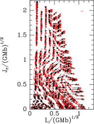
Refer to caption Refer to caption Refer to caption

Refer to caption Refer to caption Refer to caption

Figure 7: Flux vectors 𝐅¯subscript¯𝐅\overline{{\bf F}}_{\ell} in clusters with N=105𝑁superscript105N=10^{5} equal-mass particles with Ra/b=2subscript𝑅a𝑏2R_{\rm a}/b=2 (left) and 4.24.24.2 (centre), and in the isotropic model (right). The fluxes 𝐅¯1subscript¯𝐅1\overline{{\bf F}}_{1} are shown in the upper row, with the fluxes 𝐅¯2subscript¯𝐅2\overline{{\bf F}}_{2} shown below. The dressed flow is shown by red arrows on top of which are printed black arrows describing the bare flow. The length of an arrow is proportional to log10[|𝐅¯|/(1012Mb2)]subscript10¯𝐅superscript1012𝑀superscript𝑏2\log_{10}[|\overline{{\bf F}}|/(10^{-12}Mb^{-2})], so that an arrow of zero length corresponds to |𝐅¯|=1012Mb2subscript¯𝐅superscript1012𝑀superscript𝑏2|\overline{{\bf F}}_{\ell}|=10^{-12}Mb^{-2}. The bar at top right corresponds to a hundred-fold increase in |𝐅¯|subscript¯𝐅|\overline{{\bf F}}_{\ell}|.

Red arrows show the dressed (self-gravitating) flux, and black arrows show the corresponding bare flux computed by setting the response matrix Mpq=0subscript𝑀𝑝𝑞0M_{pq}=0 (i.e. with self-gravity switched off). These fluxes are obtained by summing over all pairs (𝐧~,𝐧~)~𝐧superscript~𝐧(\widetilde{\bf n},\widetilde{\bf n}^{\prime}) with n~1,n~1[2,2]subscript~𝑛1superscriptsubscript~𝑛122\widetilde{n}_{1},\widetilde{n}_{1}^{\prime}\in[-2,2]. In all three models, 𝐅¯1subscript¯𝐅1\overline{{\bf F}}_{1} generally shifts stars to lower Jrsubscript𝐽𝑟J_{r} but with a characteristic swirling action that causes L𝐿L to sometimes decreases and sometimes increase. In anisotropic models this swirling pattern is broken at the right-hand edge of the populated part of the LJr𝐿subscript𝐽𝑟LJ_{r} plane, where the restriction Q>0𝑄0Q>0 gives rise to a cliff-edge in f¯(𝐉~)¯𝑓~𝐉\overline{f}(\widetilde{\bf J}): stars naturally diffuse over this edge notwithstanding the fact that a small distance to the left of this edge stars are diffusing in almost the opposite direction. Since 𝐧~~𝐧\widetilde{\bf n} sets the direction of its contribution to 𝐅¯¯𝐅\overline{{\bf F}} (equation (50)), the swirling pattern in the upper panels of Fig. 7 indicates that the dominant value of 𝐧~~𝐧\widetilde{\bf n} changes as one moves through action space.

In Fig. 7 bare and dressed fluxes are plotted in black and red arrows, respectively, with black over-plotting red where they coincide. The length of an arrow is proportional to log10[|𝐅¯|/(1012Mb2)]subscript10¯𝐅superscript1012𝑀superscript𝑏2\log_{10}[|\overline{{\bf F}}|/(10^{-12}Mb^{-2})]. If |𝐅¯|<1012Mb2¯𝐅superscript1012𝑀superscript𝑏2|\overline{{\bf F}}|<10^{-12}Mb^{-2} no arrow is plotted, hence the blank regions in the panels. A red line at the upper right of each panel indicates how the length of an arrow increases when |𝐅¯|¯𝐅|\overline{{\bf F}}| is multiplied by 100. The shortness of this line makes clear the large dynamical range covered by 𝐅¯¯𝐅\overline{\bf F}, largely as a consequence of the large dynamic range in each model’s phase-space density f0subscript𝑓0f_{0}. In much of the upper three panels of Fig. 7 the red and black arrows are aligned but the red arrow is significantly longer. In the lower left corner arrows of each colour point in significantly different directions, indicating that the contributions from some vectors 𝐧~~𝐧\widetilde{\bf n} are amplified by self-gravity much more than others.

The strong enhancement of 𝐅¯1subscript¯𝐅1\overline{{\bf F}}_{1} by self-gravity is a natural consequence of the finding of Weinberg (1991) and Weinberg (1994) that the =11\ell=1 modes of clusters can be very weakly damped. These modes involve the cluster’s core and halo moving in antiphase along a line, so the linear momenta of the moving parts cancel. The impact of these modes on 𝐅¯1subscript¯𝐅1\overline{{\bf F}}_{1} is much enhanced by including self-gravity. Displacing the core with respect to the halo obviously becomes harder as the extent of radial anisotropy increases, and careful examination of the arrows in the upper row of Fig. 7 confirms that including self-gravity enhances 𝐅¯1subscript¯𝐅1\overline{{\bf F}}_{1} less when Ra=2bsubscript𝑅a2𝑏R_{\rm a}=2b than in the isotropic model. We note that for the secular evolution of discs the tapering of the inner and outer regions that was implemented in Fouvry et al. (2015) prevented any contributions from these =11\ell=1 modes.

The lower three panels of Fig. 7 show the fluxes 𝐅¯2subscript¯𝐅2\overline{{\bf F}}_{2}, obtained by adding the contributions of the 49 pairs (𝐧~,𝐧~)~𝐧superscript~𝐧(\widetilde{\bf n},\widetilde{\bf n}^{\prime}) with n~1[2,2]subscript~𝑛122\widetilde{n}_{1}\in[-2,2] and n~2[2,2]subscript~𝑛222\widetilde{n}_{2}\in[-2,2]. In these panels red is much less in evidence than in the upper panels, indicating that couplings associated with =22\ell=2 are less strongly affected by self-gravity than those associated with =11\ell=1. Red is most evident in the panel for Ra=2bsubscript𝑅a2𝑏R_{\rm a}=2b, as is to be expected given the vulnerability of this model to quadrupole distortions (May & Binney, 1986; Saha, 1991). In all three lower panels by far the largest =22\ell=2 fluxes occur in the bottom left corner, so physically in the cluster’s core. There the flux shifts stars to larger Jrsubscript𝐽𝑟J_{r} and smaller L𝐿L. In the nearly unstable model Ra=2bsubscript𝑅a2𝑏R_{\rm a}=2b, the flux outside this core region moves stars to smaller Jrsubscript𝐽𝑟J_{r} and larger L𝐿L, and thus tends to reduce the anisotropy that inclines the model to the radial-orbit instability.

Fig. 8 shows sums of the =11\ell=1 and =22\ell=2 fluxes.

Refer to caption Refer to caption Refer to caption

Figure 8: The result of adding the =11\ell=1 and 2 contributions to 𝐅¯¯𝐅\overline{{\bf F}}. As in Fig. 7 panels are for models with Ra=2bsubscript𝑅a2𝑏R_{\rm a}=2b (left), Ra=4.2bsubscript𝑅a4.2𝑏R_{\rm a}=4.2b (centre) and the isotropic model (right) and the arrows are scaled in the same way.

In the region of action space that is populated in all three models, the structure of the flow does not differ greatly between models. As Rasubscript𝑅aR_{\rm a} increases, the populated part of phase space extends into a region in which the flow is towards smaller L𝐿L.

Away from the cluster cores, the total fluxes are very similar to the =11\ell=1 fluxes because the latter are significantly larger than the =22\ell=2 fluxes. In the core 𝐅¯2subscript¯𝐅2\overline{{\bf F}}_{2} dominates and pushes stars to smaller L𝐿L and slightly larger Jrsubscript𝐽𝑟J_{r}. Around the core 𝐅¯1subscript¯𝐅1\overline{{\bf F}}_{1} and 𝐅¯2subscript¯𝐅2\overline{{\bf F}}_{2} are in opposite directions but the net flow reduces Jrsubscript𝐽𝑟J_{r}. In the model with Ra=2bsubscript𝑅a2𝑏R_{\rm a}=2b the flow generally increases L𝐿L, thus diminishing the model’s radial anisotropy.

We find the largest of 𝐅¯0subscript¯𝐅0\overline{{\bf F}}_{0}, 𝐅¯3subscript¯𝐅3\overline{{\bf F}}_{3} and 𝐅¯4subscript¯𝐅4\overline{{\bf F}}_{4} is always smaller than 𝐅¯2subscript¯𝐅2\overline{{\bf F}}_{2}, so we do not present our values for them.

Fig. 9 plots f¯/t¯𝑓𝑡\partial\overline{f}/\partial t for the models with Ra/b=2subscript𝑅a𝑏2R_{\rm a}/b=2 and 4.24.24.2 (left and centre) and the isotropic model (right) computed from the divergence of the dressed BL fluxes plotted in Fig. 8.
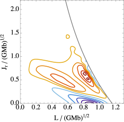
Refer to caption Refer to caption Refer to caption


Figure 9: The rate of change of the DF, f¯/t=/𝐉~𝐅¯¯𝑓𝑡~𝐉¯𝐅\partial\overline{f}/\partial t=-\partial/\partial\widetilde{\bf J}\cdot\overline{\bf F} for the models with Ra=2bsubscript𝑅a2𝑏R_{\rm a}=2b (left), Ra=4.2bsubscript𝑅a4.2𝑏R_{\rm a}=4.2b (centre) and the isotropic model (right). These rates are minus the divergence of the dressed BL fluxes. Red contours indicate that f¯¯𝑓\overline{f} is decreasing, blue that it is increasing. The boundary of the allowed action space domain is represented by the heavy black line.

The red contours indicate regions in which f¯¯𝑓\overline{f} is decreasing, while blue contours mark regions in which it is increasing. The data are quite noisy because they involve differentiation of the numerically computed fluxes. However, in all three models f¯¯𝑓\overline{f} increases at Jr0similar-to-or-equalssubscript𝐽𝑟0J_{r}\simeq 0 and LGMbsimilar-to-or-equals𝐿𝐺𝑀𝑏L\simeq\sqrt{GMb} and decreases at high Jrsubscript𝐽𝑟J_{r} and small L𝐿L. In order to illustrate the variety of diffusion features that can generically arise from the BL equation, in Appendix A we briefly consider the case of a tangentially anisotropic DF and illustrate again how self-gravity may impact the properties of the orbital diffusion.

6 Comparison with classical theory

Let us now compare the results of the BL formalism to those of the classical (Spitzer–Chandrasekhar) theory of local scattering. In Appendix B we show that classical theory predicts

f¯t=i=12Ji(F¯1i+F¯2i),¯𝑓𝑡superscriptsubscript𝑖12subscript𝐽𝑖superscriptsubscript¯𝐹1𝑖superscriptsubscript¯𝐹2𝑖{\partial\overline{f}\over\partial t}=-\sum_{i=1}^{2}{\partial\over\partial J_{i}}(\overline{F}_{1}^{i}+\overline{F}_{2}^{i}), (81)

where the fluxes 𝐅¯isubscript¯𝐅𝑖\overline{\bf F}_{i} are given by

F¯1isuperscriptsubscript¯𝐹1𝑖\displaystyle\overline{F}_{1}^{i} =(2π)2f¯dθrdψ[Di12ΓjniDjn]absentsuperscript2𝜋2¯𝑓differential-dsubscript𝜃𝑟differential-d𝜓delimited-[]superscript𝐷𝑖12subscriptsuperscriptΓ𝑖𝑗𝑛superscript𝐷𝑗𝑛\displaystyle=(2\pi)^{-2}\overline{f}\int{\rm d}\theta_{r}\,{\rm d}\psi\,\Bigl{[}D^{i}-{\textstyle{1\over 2}}\Gamma^{i}_{jn}D^{jn}\Bigr{]} (82)
F¯2isuperscriptsubscript¯𝐹2𝑖\displaystyle\overline{F}_{2}^{i} =12(2π)2Jj(f¯dθrdψDij),absent12superscript2𝜋2subscript𝐽𝑗¯𝑓differential-dsubscript𝜃𝑟differential-d𝜓superscript𝐷𝑖𝑗\displaystyle=-{\textstyle{1\over 2}}(2\pi)^{-2}{\partial\over\partial J_{j}}\biggl{(}\overline{f}\int{\rm d}\theta_{r}\,{\rm d}\psi\,D^{ij}\biggr{)}, (83)

(here we are using the summation convention over repeated indices). Here Disuperscript𝐷𝑖D^{i} and Djnsuperscript𝐷𝑗𝑛D^{jn} are rates of change of expectation values that can be obtained from the Rosenbluth potentials (Rosenbluth et al., 1957), ΓjnisubscriptsuperscriptΓ𝑖𝑗𝑛\Gamma^{i}_{jn} is a Christoffel symbol that emerges from the functional dependence of the actions on velocity, and θrsubscript𝜃𝑟\theta_{r} and ψ𝜓\psi are angles appearing in this dependence.

Evaluation of the Rosenbluth potentials for an anisotropic velocity distribution is costly, so, as is standard practice in studies of globular-cluster evolution (e.g. Cohn, 1979; Drukier et al., 1999), we evaluate the Rosenbluth potentials using an equivalent ergodic DF

fiso(E,r)=01dcf(E,r2vE22Ra2(1c2)),subscript𝑓iso𝐸𝑟superscriptsubscript01differential-d𝑐𝑓𝐸superscript𝑟2subscriptsuperscript𝑣2E2superscriptsubscript𝑅a21superscript𝑐2f_{\rm iso}(E,r)=\int_{0}^{1}{\rm d}c\,f\left(E,{r^{2}v^{2}_{\rm E}\over 2R_{\rm a}^{2}}(1-c^{2})\right), (84)

where vE(r)subscript𝑣E𝑟v_{\rm E}(r) is the speed at r𝑟r of a particle of energy E𝐸E. After computing the Rosenbluth potentials with fisosubscript𝑓isof_{\rm iso}, the appropriate anisotropic DF f¯¯𝑓\overline{f} is used in equations (82) for the flux.

Fig. 10 shows for two finite values of Rasubscript𝑅aR_{\rm a}, namely Ra=2bsubscript𝑅a2𝑏R_{\rm a}=2b and 4.2b4.2𝑏4.2b, and for the isotropic model, the resulting classical flux vectors scaled as in Figs. 7 and 8 for a cluster of N=105𝑁superscript105N=10^{5} equal-mass stars under the assumption that lnΛ=8.9Λ8.9\ln\Lambda=8.9 (Section B.1).

Refer to caption Refer to caption Refer to caption

Figure 10: Flux through 𝐉~~𝐉\widetilde{\bf J} space, 𝐅¯(𝐉~)¯𝐅~𝐉\overline{{\bf F}}(\widetilde{\bf J}), computed using the local approximation for models with Ra=2bsubscript𝑅a2𝑏R_{\rm a}=2b (left), 4.2b4.2𝑏4.2b (centre) and the isotropic model (right). The length of an arrow is proportional to log10[|𝐅¯|/(1012Mb2)]subscript10¯𝐅superscript1012𝑀superscript𝑏2\log_{10}[|\overline{{\bf F}}|/(10^{-12}Mb^{-2})], so that an arrow of zero length corresponds to |𝐅¯|=1012Mb2¯𝐅superscript1012𝑀superscript𝑏2|\overline{{\bf F}}|=10^{-12}Mb^{-2} as in Fig. 7. The red bar at top right corresponds to a hundred-fold increase in |𝐅¯|¯𝐅|\overline{{\bf F}}|.

The flow is structured by stagnation points. For Ra=2bsubscript𝑅a2𝑏R_{\rm a}=2b there is a single stagnation point that lies on the Jrsubscript𝐽𝑟J_{r} axis at Jr2.0GMbsimilar-tosubscript𝐽𝑟2.0𝐺𝑀𝑏J_{r}\sim 2.0\sqrt{GMb}. This point moves down the Jrsubscript𝐽𝑟J_{r} axis as Rasubscript𝑅aR_{\rm a} increases, so that by Ra=4.2bsubscript𝑅a4.2𝑏R_{\rm a}=4.2b it is at Jr0.6GMbsimilar-tosubscript𝐽𝑟0.6𝐺𝑀𝑏J_{r}\sim 0.6\sqrt{GMb}. The Ra=4.2bsubscript𝑅a4.2𝑏R_{\rm a}=4.2b plot also shows signs of another stagnation point on the L𝐿L axis, roughly at L0.1(GMb)1/2similar-to𝐿0.1superscript𝐺𝑀𝑏12L\sim 0.1(GMb)^{1/2} (see Appendix B.2). For larger Rasubscript𝑅aR_{\rm a} we have a single stagnation point on the L𝐿L axis, where it sticks as Rasubscript𝑅aR_{\rm a} tends to infinity. Above the stagnation point and near the Jrsubscript𝐽𝑟J_{r} axis the flow is vertically upwards, while below the stagnation point the flow is to lower Jrsubscript𝐽𝑟J_{r} and higher L𝐿L.

The classical flow pattern for the model with Ra=2bsubscript𝑅a2𝑏R_{\rm a}=2b is not unlike that obtained from the BL equation (left panel of Fig. 8). Given that in computing the BL fluxes we have only included the =1,212\ell=1,2 terms and confined ourselves to wave vectors 𝐧~~𝐧\widetilde{\bf n} with n~1[2,2]subscript~𝑛122\widetilde{n}_{1}\in[-2,2], the extent of the agreement between the two panels on the left of Fig. 8 and the corresponding panels of Fig. 10 is remarkable. As we proceed to larger Rasubscript𝑅aR_{\rm a}, the differences between the classical and the BL flows becomes pronounced. In the isotropic model the BL flow is everywhere towards smaller Jrsubscript𝐽𝑟J_{r} whereas the classical flow is towards larger Jrsubscript𝐽𝑟J_{r}. The tendency of the classical flow to increase Jrsubscript𝐽𝑟J_{r} is consistent with the well known tendency of the halos of clusters to become radially biased.

Fig. 11 shows the rate of change of the DF f¯/t¯𝑓𝑡\partial\overline{f}/\partial t (in units of M/Gb5𝑀𝐺superscript𝑏5\sqrt{M/Gb^{5}}) for the models with Ra/b=2subscript𝑅a𝑏2R_{\rm a}/b=2 and 4.24.24.2 (left and centre) and the isotropic model (right), all computed from the divergence of the classical flux vectors shown in Fig. 10.
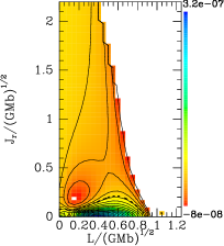
Refer to caption Refer to caption Refer to caption

Figure 11: The rate of change of the DF, f¯/t=/𝐉~𝐅¯¯𝑓𝑡~𝐉¯𝐅\partial\overline{f}/\partial t=-\partial/\partial\widetilde{\bf J}\cdot\overline{\bf F}, computed in the local approximation for the model with Ra=2bsubscript𝑅a2𝑏R_{\rm a}=2b (left), Ra=4.2bsubscript𝑅a4.2𝑏R_{\rm a}=4.2b (centre), and for the isotropic model (right). In each case we plot 20 solid contours, spaced linearly from the minimum to maximum value of (f¯/t)/M/Gb5¯𝑓𝑡𝑀𝐺superscript𝑏5(\partial\overline{f}/\partial t)/\sqrt{M/Gb^{5}}. The dashed contours divide regions of increasing and decreasing phase-space density.

In each panel the dashed contour divides the regions in which the DF is increasing from those at which it is decreasing. Whereas in the isotropic model 𝐅¯¯𝐅\overline{\bf F} tends to shift stars from nearly circular orbits to more eccentric ones, in the highly anisotropic model Ra=2bsubscript𝑅a2𝑏R_{\rm a}=2b the portion of action space associated with eccentric orbits is depopulated to feed growth in the region associated with nearly circular orbits.

Fig. 12 compares the magnitudes of the BL fluxes in each panel of Fig. 8 to the classical fluxes plotted in Fig. 10.
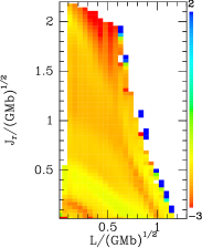
Refer to caption Refer to caption Refer to caption

Refer to caption Refer to caption Refer to caption

Figure 12: Ratios of the magnitudes of BL fluxes to classical fluxes. Upper row: bare fluxes; lower row: dressed fluxes. The left and central panels are for the models with Ra=2bsubscript𝑅a2𝑏R_{\rm a}=2b and 4.2b4.2𝑏4.2b, respectively, while the right panel is for the isotropic model. The colour scales shows log10(|𝐅BL|/|𝐅Class|)subscript10subscript𝐅BLsubscript𝐅Class\log_{10}(|{\bf F}_{\rm BL}|/|{\bf F}_{\rm Class}|).

The upper row is for the bare fluxes while the lower row is for dressed fluxes. The colour scales indicate logarithms to base 10 of the ratio of the BL flux to the classical flux. Whereas the bare BL fluxes are almost everywhere significantly smaller than the classical fluxes, outside the core the dressed fluxes are as large as or larger than the classical fluxes. The BL fluxes, both bare and dressed, tend to increase relative to the classical fluxes as Rasubscript𝑅aR_{\rm a} increases.

7 Discussion

Chavanis (2013a) (see also Chavanis, 2013b) has shown that the BL equation yields the classical theory of relaxation when one neglects inhomogeneity and collective effects. Indeed, in the limit of a homogeneous system, the three components of velocity take on the role of actions, the Cartesian coordinates xisubscript𝑥𝑖x_{i}, which increase uniformly along unperturbed trajectories, play the role of angles, and the sum over discrete vectors 𝐧𝐧{\bf n} becomes an integral over wavevectors. Neglect of collective effects enables one to execute this integral and recover the classical theory. Thus there is little doubt that if we could sum over all resonating pairs (𝐧~,𝐧~)~𝐧superscript~𝐧(\widetilde{\bf n},\widetilde{\bf n}^{\prime}) and all \ell, we would obtain a flux that embraced the classical flux but went beyond it in that (i) our flux would include the impact of large-scale amplified fluctuations that are not properly handled in the classical theory, and (ii) the flux would not depend on an ill-determined parameter such as logΛΛ\log\Lambda.

Since collective effects should be unimportant on small scales, it follows from Chavanis’ work that for some choice of logΛΛ\log\Lambda, classical theory should yield a good approximation to the portion of the diffusive flux that arises from encounters at small impact parameters – we shall refer to this as the ‘small-scale’ BL flux. With our current computational machinery it is not feasible to compute the small-scale BL flux by summing to high \ell and/or high |n~1|subscript~𝑛1|\widetilde{n}_{1}| or |n~2|subscript~𝑛2|\widetilde{n}_{2}|. Hence our BL fluxes arise exclusively from the part of the BL sum that returns the flux driven by interactions between stars for which the local approximation of classical theory is certainly invalid.

For our comparison to the classical flux we have used N=105𝑁superscript105N=10^{5}. The BL flux is proportional to the mass μ𝜇\mu of a star and therefore scales with the number of particles like 1/N1𝑁1/N (Section 3). The classical flux is proportional to μlogΛ𝜇Λ\mu\log\Lambda (Appendix B) and so scales like lnN/N𝑁𝑁\ln N/N. Therefore the ratio of BL to classical flux scales with particle number like 1/lnN1𝑁1/\ln N.

Given the ill-defined value of the Coulomb logarithm, the magnitude of the classical flux is uncertain. We have adopted logΛ=8.9Λ8.9\log\Lambda=8.9, to get an idea of the magnitude of the small-scale BL flux. Our key finding is that, when the cluster’s self-gravity is taken into account, the large-scale BL flux is as large as or even larger than the small-scale flux. Including self-gravity dramatically increases the diffusion generated by thermal excitation of the weakly damped, low frequency =11\ell=1 mode of clusters. This finding makes perfect sense physically, because this mode involves the cluster’s core and envelope oscillating in antiphase and periodically exchanging momentum. If the stars move in a fixed gravitational field, this mode of communication is impractical because the core then oscillates at a much higher frequency than the halo, and each section will exchange momentum with the source of the fixed gravitational field rather than the other half of the cluster.

When there are many orbits that move between the core and the halo, it will be harder for the core and the halo to oscillate in antiphase, so the =11\ell=1 mode will be harder to excite. Hence for such modes it is natural that the magnitude of the large-scale BL flux relative to that of the small-scale flux is decreased by making the cluster radially anisotropic.

It is well known that as radial anisotropy increases the energy required to make a cluster prolate decreases, and at a critical level of anisotropy it vanishes so the cluster is liable to spontaneous bar formation. Our results confirm the view of May & Binney (1986) that the critical level of anisotropy is reached near Ra=1.7bsubscript𝑅a1.7𝑏R_{\rm a}=1.7b. We find, as expected, that the =22\ell=2 contribution to the dressed BL flux associated with quadrupole symmetry increases as Rasubscript𝑅aR_{\rm a} decreases through thermal excitation of the quadrupole mode. We have not, however, computed a model that is sufficiently close to the critical anisotropy for the enhancement by self-gravity to be comparable to that found for the =11\ell=1 contribution to the flux in every model.

We have found that contributions to 𝐅¯¯𝐅\overline{{\bf F}} from =0,3,4034\ell=0,3,4 are much smaller than contributions from =1,212\ell=1,2. From these conclusions it does not follow that it was legitimate to neglect these and other 𝐅¯subscript¯𝐅\overline{{\bf F}}_{\ell}, nor does the large magnitude of our dressed BL fluxes justify limiting the sums over wavevectors to small 𝐧~~𝐧\widetilde{\bf n}. Indeed, classical theory, which consists of an approximate summation over the neglected terms, strongly suggests that the terms we have dropped are collectively important. Each wavevector 𝐧~~𝐧\widetilde{\bf n} in the sum contributes a flux in its own unique direction. The direction of our BL flux is set by the vectors 𝐧~~𝐧\widetilde{\bf n} we have chosen to include, while the classical flux is the result of summing over an infinite number of vectors, and in consequence it can point in a radically different direction, as comparison of the panels on the right of Figs. 8 and 10 shows to be the case in the isotropic model.

This discussion suggests that the partial BL summation on the one hand and the classical theory on the other hand provide distinct approximations to the flux. A summation over the leading discrete 𝐧~~𝐧\widetilde{\bf n}, combined with summation over a myriad of other 𝐧~~𝐧\widetilde{\bf n} that make small individual contributions to the flux may eventually prove sufficient (Weinberg, 1986). Most of these small contributions are expected to come from small-scale fluctuations in the potential that are probably adequately modelled by the orbit-averaged classical theory because neither inhomogeneity nor collective effects are important on small scales. Consequently, a proper procedure may involve computing the dominant terms in the dressed BL expressions for the diffusion coefficients and approximating the remaining infinite sum by the classical diffusion coefficients using a smaller value of logΛΛ\log\Lambda. The remaining problems are (i) expediting the computation of the BL terms, which is unreasonably costly with our current code and (ii) estimating the correct value of logΛΛ\log\Lambda.

7.1 N-body simulations

If classical theory is so misleading, why have N-body simulations of cluster relaxation not exposed this fact? A likely answer has two parts. First, classical theory has the free parameter logΛΛ\log\Lambda, and second analysis of N-body simulations is hard and the action-space flux 𝐅¯¯𝐅\overline{{\bf F}} is rarely computed. Rather the rate at which the model’s radial density profile evolves is computed, and logΛΛ\log\Lambda is adjusted to make the classically predicted rate agree with the measured rate. Theuns (1996) did compute the rate at which particles in N-body clusters (in this case isotropic King models) diffused in energy. He concluded that on average they diffused about twice as fast as classical theory predicted, and that outside the core classical theory underestimated the size of the the dynamical friction coefficient by up to a factor of 101010. These conclusions are roughly in agreement with the lower-right panel of our Fig. 12. Additionally, the excess power due to large scale modes has been seen in N-body simulations (for example those of Weinberg (1998); see also Weinberg (2001)). The patterns of the weakly damped modes themselves might simply be too hard to see in real space because they have such low frequencies and are soon washed out by noise (Weinberg, 2001). Sellwood (2015) performed N-body simulations of homogeneous spheres and found a scaling of the energy relaxation with N𝑁N which strongly suggested the dominance of large-scale collective modes driven by Poisson noise. On the other hand, Sellwood (2015) also simulated Hernquist and Plummer spheres and found fairly good agreement with the classical picture. The changes to the relaxation rate that can result from tuning logΛΛ\log\Lambda to any sensible value are typically only 1020%similar-toabsent10percent20\sim 10-20\% and so this alone cannot account for the consistent agreement which has been found between N-body and Fokker-Planck models. Finally we note that Kim et al. (2008) measured a significantly smaller discrepancy in energy diffusion rate from the classical expectation than Theuns (1996).

The validity of our conclusions should be tested by direct N-body simulations of clusters. A suitable programme would comprise an ensemble of short simulations of isochrone clusters. Individual simulations could be integrated for times significantly shorter than the half-mass relaxation time, so their mean-field potentials would remain close to that of the isochrone, and the actions of particles could be readily computed. By comparing actions computed at successive timesteps, fluxes across a grid of lines in LJr𝐿subscript𝐽𝑟LJ_{r} space could be determined. Moreover, the difference between the actual potential and the isochrone potential, projected onto a set of basis functions ΦnmsubscriptΦ𝑛𝑚\Phi_{n\ell m} could be monitored so one could estimate how much of the flux is generated by large-scale fluctuations that are significantly enhanced by self-gravity and cannot be well described by classical theory. Good statistics would be accumulated by stacking results from simulations that differed only in their initial conditions. We plan to present the results of such a study in the near future.

8 Conclusions

The classical theory of relaxation in star clusters has for decades formed one of the pillars of stellar dynamics. Yet it is well known to rest on shaky foundations in that its predictions all involve integrals that diverge logarithmically at large impact parameters. Conventionally this divergence is mastered by imposing an upper limit on impact parameters. Predictions then become proportional to the logarithm of this cutoff, so the theory has a free parameter.

A further weakness of the classical theory is that it neglects the cluster’s self-gravity. In Section 2 we gave a back-of-the-envelope argument that by accounting for Poisson fluctuations alone one can recover the classical expression for the relaxation time. Since self-gravity makes a star cluster more compressible than an ideal gas it follows that slow, large-scale fluctuations in density are liable to drive a cluster to relax faster than classical theory predicts.

In two important papers Weinberg (1993, 1998) presented arguments that the self-gravity significantly speeds the relaxation of stellar systems through excitation of large-scale modes. However, he did not provide an equation for the secular evolution of the DF when large-scale modes and self-gravity are properly handled. Such an equation, derived from a rigorous, self-consistent theory of relaxation that contains no arbitrary constants, appeared first in Heyvaerts (2010). The structure of this ‘BL equation’ suggests a physical picture of how systems relax that is radically different from the classical picture of successive stellar encounters. In Section 3 we summarised this theory, and in Section 4 we modified it so it could be applied to spherical systems, which have a degeneracy that precludes application of the unmodified equation.

According to the new theory, relaxation does not occur through localised encounters between stars but through pairs of stars communicating with each other by shaking the entire system at a specific frequency ω𝜔\omega. The stars do not need to be near each other in real space, although proximity will make communication easier. The effectiveness of communication between stars depends also on whether they can communicate at a frequency that lies near a weakly damped mode of the entire system. Self-gravity is important because it determines the modal structure. Fouvry et al. (2015) applied the new theory to stellar discs and showed that it could for the first time explain the emergence of strong spiral structure in N-body simulations of linearly stable discs. In particular, they showed that when self-gravity is properly included, realistic stellar discs can relax 1000similar-toabsent1000\sim 1000 times faster than classical theory predicts. Moreover, through a mechanism proposed by Sellwood & Carlberg (2014), the resonant nature of the disc’s relaxation steers the disc to a configuration in which it is unstable as a collisionless system, so it eventually develops a strong bar on a dynamical timescale.

In Section 5 we put forward the first implementation of the BL theory to three spherical clusters that all have the spatial structure of Hénon’s isochrone but distribution functions with different degrees of radial velocity anisotropy. The problem one encounters is the need to sum over infinitely many resonant interactions, each defined by a pair of two-dimensional vectors 𝐧~,𝐧~~𝐧superscript~𝐧\widetilde{\bf n},\widetilde{\bf n}^{\prime} with integer components. We tried to identify, and then sum, the interactions that make the largest contributions. The sum can be partitioned into contributions from each angular momentum quantum number \ell, and we considered =0,,404\ell=0,\ldots,4. We found that the sums for =1,212\ell=1,2 dominate strongly. However, the number of vector pairs that could contribute significantly grows rapidly with \ell and the size of the vectors, and it is possible for some configurations that large numbers of interactions that individually contribute little together contribute as much as the most important interactions (Weinberg, 1986). This being so, our partial sum may under-estimate the magnitude of the BL flux through phase space. In all three clusters, the partial BL fluxes are much larger when self-gravity is included than otherwise. This is to be expected because the terms we have included arise from large-scale distortions of the cluster, which are precisely the fluctuations enhanced by self-gravity.

In Appendix B we recovered the fluxes predicted by classical theory. In Section 6 we compared these fluxes with our partial BL fluxes. In the isotropic cluster, the fluxes have quite different directions, and the classical flux is often larger than the bare partial BL flux, consistent with our having missed the contributions of myriads of interactions that individually contribute little. The dressed partial BL fluxes are, by contrast, often larger than the classical flux, suggesting that the classical flux significantly under-estimates the rate of relaxation. The dominance of the dressed BL flux over the classical flux is most pronounced in the isotropic cluster and at large L𝐿L.

We conclude that classical theory is liable to under-estimate the rate of relaxation through neglect of self-gravity and non-local resonances. Whereas this can lead to the relaxation rate of a stellar disc being under-estimated by a factor 1000similar-toabsent1000\sim 1000, for a spherical system the magnitude of the relaxation rate predicted by (large scale) BL theory is typically similar-to\sim a few times that of classical theory (but is often in a completely different direction and can be significantly larger depending on the anisotropy of the cluster). However, brute-force application of the BL equation may not yet provide a fully viable alternative to classical theory because of the evaluation of the infinite sum over interaction vectors. A way must be found to combine a sum over the most important resonance vectors, which are associated with large-scale fluctuations and the important effects of self-gravity, with an integral like that executed in classical theory to include the effects of small-scale fluctuations, to which self-gravity contributes little. However, we should first confirm our finding that classical theory misses out some important physics through analysis of tailored N-body simulations.

Acknowledgements

JJB is supported by the European Research Council under the European Union’s Seventh Framework Programme (FP7/2007-2013)/ERC grant agreement no. 321067. JBF acknowledges support from Program number HST-HF2-51374 which was provided by NASA through a grant from the Space Telescope Science Institute, which is operated by the Association of Universities for Research in Astronomy Incorporated, under NASA contract NAS5–26555. This research was in part carried out within the framework of the Spin(e) collaboration (ANR-13-BS05-0005 http://cosmicorigin.org)

References

  • An & Evans (2006) An J. H., Evans N. W., 2006, AJ, 131, 782
  • Balescu (1960) Balescu R., 1960, Physics of Fluids, 3, 52
  • Binney & Tremaine (2008) Binney J., Tremaine S., 2008, Galactic Dynamics: Second Edition. Princeton University Press
  • Carroll (2004) Carroll S. M., 2004, Spacetime and geometry. An introduction to general relativity
  • Chandrasekhar (1943) Chandrasekhar S., 1943, ApJ, 97, 255
  • Chandrasekhar (1949) Chandrasekhar S., 1949, Reviews of Modern Physics, 21, 383
  • Chavanis (2012) Chavanis P.-H., 2012, Physica A, 391, 3680
  • Chavanis (2013a) Chavanis P.-H., 2013a, European Physical Journal Plus, 128, 126
  • Chavanis (2013b) Chavanis P.-H., 2013b, A&A, 556, A93
  • Clutton-Brock (1973) Clutton-Brock M., 1973, ApSpSc, 23, 55
  • Cohn (1979) Cohn H., 1979, ApJ, 234, 1036
  • Drukier et al. (1999) Drukier G. A., Cohn H. N., Lugger P. M., Yong H., 1999, The Astrophysical Journal, 518, 233
  • Edmonds (1996) Edmonds A., 1996, Angular Momentum in Quantum Mechanics. Princeton University Press
  • Fouvry et al. (2017) Fouvry J.-B., Pichon C., Magorrian J., 2017, A&A, 598, A71
  • Fouvry et al. (2015) Fouvry J. B., Pichon C., Magorrian J., Chavanis P. H., 2015, A&A, 584, A129
  • Fridman & Poliachenko (1984) Fridman A. M., Poliachenko V. L., 1984, Physics of gravitating systems. II. Springer-Verlag Berlin Heidelberg
  • Henon (1959) Henon M., 1959, Annales d’Astrophysique, 22, 126
  • Hénon (1960) Hénon M., 1960, Annales d’Astrophysique, 23, 474
  • Hernquist & Ostriker (1992) Hernquist L., Ostriker J. P., 1992, ApJ, 386, 375
  • Heyvaerts (2010) Heyvaerts J., 2010, MNRAS, 407, 355
  • Kalnajs (1976) Kalnajs A. J., 1976, ApJ, 205, 745
  • Kim et al. (2008) Kim E., Yoon I., Lee H. M., Spurzem R., 2008, Monthly Notices of the Royal Astronomical Society, 383, 2
  • Lenard (1960) Lenard A., 1960, Annals of Physics, 10, 390
  • May & Binney (1986) May A., Binney J., 1986, MNRAS, 221, 13P
  • Palmer & Papaloizou (1987) Palmer P. L., Papaloizou J., 1987, MNRAS, 224, 1043
  • Rahmati & Jalali (2009) Rahmati A., Jalali M. A., 2009, MNRAS, 393, 1459
  • Rauch & Tremaine (1996) Rauch K. P., Tremaine S., 1996, NAstr, 1, 149
  • Rosenbluth et al. (1957) Rosenbluth M. N., MacDonald W. M., Judd D. L., 1957, Physical Review, 107, 1
  • Saha (1991) Saha P., 1991, MNRAS, 248, 494
  • Sellwood (2015) Sellwood J. A., 2015, MNRAS, 453, 2919
  • Sellwood & Carlberg (2014) Sellwood J. A., Carlberg R. G., 2014, ApJ, 785, 137
  • Theuns (1996) Theuns T., 1996, MNRAS, 279, 827
  • Tremaine & Weinberg (1984) Tremaine S., Weinberg M. D., 1984, MNRAS, 209, 729
  • Weinberg (1986) Weinberg M. D., 1986, ApJ, 300, 93
  • Weinberg (1989) Weinberg M. D., 1989, MNRAS, 239, 549
  • Weinberg (1991) Weinberg M. D., 1991, ApJ, 368, 66
  • Weinberg (1993) Weinberg M. D., 1993, ApJ, 410, 543
  • Weinberg (1994) Weinberg M. D., 1994, ApJ, 421, 481
  • Weinberg (1998) Weinberg M. D., 1998, MNRAS, 297, 101
  • Weinberg (2001) Weinberg M. D., 2001, in Woodward C. E., Bicay M. D., Shull J. M., eds, Tetons 4: Galactic Structure, Stars and the Interstellar Medium Vol. 231 of Astronomical Society of the Pacific Conference Series, The Milky Way as a Key to Structural Evolution in Galaxies. p. 53

Appendix A Tangentially biased distribution functions

The self-consistent isochrone DF introduced in equation (61) is radially anisotropic. Following An & Evans (2006), a tangentially biased DF for the isochrone potential is given by

f0(E,L)=p(E)+q(E)L2,subscript𝑓0𝐸𝐿𝑝𝐸𝑞𝐸superscript𝐿2f_{0}(E,L)=p(E)+q(E)L^{2}, (85)

where

p(E)=𝑝𝐸absent\displaystyle p(E)= 3M(1E)4215/2π3(GMb)3/2((16E212E+3)15sin1E1E\displaystyle\,\frac{3M(1\!-\!E^{\prime})^{-4}}{2^{15/2}\pi^{3}(GMb)^{3/2}}\left(\!(16E^{\prime 2}\!-\!12E^{\prime}\!+\!3)\frac{15\sin^{-1}\!\sqrt{E^{\prime}}}{\sqrt{1-E^{\prime}}}\right.
(45150E+144E2208E3+64E4)E),\displaystyle\,\left.-(45-150E^{\prime}+144E^{\prime 2}-208E^{\prime 3}+64E^{\prime 4})\sqrt{E^{\prime}}\right),

and

q(E)=𝑞𝐸absent\displaystyle q(E)= 3M(1E)5215/2π3(GMb)3/2((40E224E+5)15sin1E1E\displaystyle\,\frac{3M(1\!-\!E^{\prime})^{-5}}{2^{15/2}\pi^{3}(GMb)^{3/2}}\left(\!(40E^{\prime 2}\!-\!24E^{\prime}\!+\!5)\frac{15\sin^{-1}\!\sqrt{E^{\prime}}}{\sqrt{1-E^{\prime}}}\right.
(75310E+400E2928E3+576E4128E5)E),\displaystyle\!\!\!\!\!\!\!\!\!\!\!\!\!\left.-(75\!-\!310E^{\prime}\!+\!400E^{\prime 2}\!-\!928E^{\prime 3}\!+\!576E^{\prime 4}\!-\!128E^{\prime 5})\sqrt{E^{\prime}}\right),

and EbE/GMsuperscript𝐸𝑏𝐸𝐺𝑀{E^{\prime}\equiv-bE/GM}. As emphasised in the BL equation (4), we may consider the averaged DF, f¯(Jr,L)=2Lf0¯𝑓subscript𝐽𝑟𝐿2𝐿subscript𝑓0\overline{f}(J_{r},L)=2Lf_{0}. In Fig. 13, we illustrate the respective contributions of the =11\ell=1 and =22\ell=2 to the diffusion flux, with and without collective effects.

Refer to caption Refer to caption

Refer to caption Refer to caption

Figure 13: The rate of change of the DF f¯/t=𝐅¯/𝐉~¯𝑓𝑡subscript¯𝐅~𝐉{\partial\overline{f}/\partial t=-\partial\overline{\bf F}_{\ell}/\partial\widetilde{\mathbf{J}}} for the tangentially anistropic DF from equation (85), for =11\ell=1 (top row) and =22\ell=2 (bottom row), without collective effects (left column) and with collective effects (right column). The convention used is the same as in Fig. 9. In the top-right panel, the dashed gray line is aligned with direction (1,1)11(-1,1).

In the first row of Fig. 13, we note the importance of collective effects in amplifying the flux and altering its direction for the =11\ell=1 component, as induced by the existence of a weakly damped =11\ell=1 mode in these systems (Weinberg, 1994). In particular, in the top-right panel, the diffusion takes place predominantly along the direction (1,1)11(-1,1). In the tangentially anisotropic model, stars are being picked up and moved along the (1,1)11(-1,1) line. Indeed, for perfectly circular orbits, one has (1,1)~𝛀=011~absent𝛀0(-1,1)\cdot\widetilde{}\mbox{\boldmath$\Omega$}=0. As there are numerous almost-circular orbits in this model, many stars will have a characteristic frequency 𝐧~~𝛀0similar-to-or-equals~𝐧~absent𝛀0\widetilde{\bf n}\cdot\widetilde{}\mbox{\boldmath$\Omega$}\simeq 0. Hence, many pairs of stars will have matching frequencies, allowing them to interact resonantly. The direction of the flux is then along the the most strongly-amplified resonance vector 𝐧~~𝐧\widetilde{\bf n}, which in this case is (1,1)11(-1,1). On the contrary, in the bottom row of Fig. 13, we note that collective effects do not boost the amplitude of the 𝐅¯2subscript¯𝐅2\overline{\bf F}_{2} flux, because the tangential model has so few radial orbits, i.e. so few orbits prone to undergo a strong self-gravitating amplification via the =22\ell=2 response.

Appendix B Classical diffusion coefficients

We use classical Spitzer–Chandrasekhar theory to compute the diffusive action-space flux. Our strategy is as follows. At each phase of an orbit of given (Jr,L)subscript𝐽𝑟𝐿(J_{r},L) we compute the probability flux and then average this flux over orbital phase. We obtain the flux at a given location by transforming the classical velocity-space Fokker-Planck equation to curvilinear coordinates for velocity-space that include Jrsubscript𝐽𝑟J_{r} and L𝐿L. The requisite tensor calculus is found in e.g. Carroll (2004).

We use as our velocity-space coordinates 𝐏=(Jr,L,ψ)𝐏subscript𝐽𝑟𝐿𝜓{\bf P}=(J_{r},L,\psi), where ψ𝜓\psi is the angle between the tangential component of the velocity and a fixed direction 𝐞xsubscript𝐞𝑥{\bf e}_{x} in the plane perpendicular to the current position vector 𝐫𝐫{\bf r}. In terms of the new velocity coordinates the Cartesian components of velocity are

(vr,vx,vy)subscript𝑣𝑟subscript𝑣𝑥subscript𝑣𝑦\displaystyle(v_{r},v_{x},v_{y}) =(2(EΦ)L2/r2,Lrcosψ,Lrsinψ),absent2𝐸Φsuperscript𝐿2superscript𝑟2𝐿𝑟𝜓𝐿𝑟𝜓\displaystyle=\left(\sqrt{2(E-\Phi)-L^{2}/r^{2}},{L\over r}\cos\psi,{L\over r}\sin\psi\right),

where E=E(Jr,L)𝐸𝐸subscript𝐽𝑟𝐿E=E(J_{r},L), so

𝐋=(0,Lsinψ,Lcosψ).𝐋0𝐿𝜓𝐿𝜓{\bf L}=(0,-L\sin\psi,L\cos\psi). (86)

Given that dE=ΩrdJr+ΩϑdLd𝐸subscriptΩ𝑟dsubscript𝐽𝑟subscriptΩitalic-ϑd𝐿{\rm d}E=\Omega_{r}{\rm d}J_{r}+\Omega_{\vartheta}{\rm d}L it follows that

dvr=ΩrdJr+(ΩϑL/r2)dLvr.dsubscript𝑣𝑟subscriptΩ𝑟dsubscript𝐽𝑟subscriptΩitalic-ϑ𝐿superscript𝑟2d𝐿subscript𝑣𝑟{\rm d}v_{r}={\Omega_{r}{\rm d}J_{r}+(\Omega_{\vartheta}-L/r^{2}){\rm d}L\over v_{r}}. (87)

Hence,

𝐯𝐏=(ΩrvrΩϑL/r2vr00cosψrvtsinψ0sinψrvtcosψ).𝐯𝐏matrixsubscriptΩ𝑟subscript𝑣𝑟subscriptΩitalic-ϑ𝐿superscript𝑟2subscript𝑣𝑟00𝜓𝑟subscript𝑣𝑡𝜓0𝜓𝑟subscript𝑣𝑡𝜓{\partial{\bf v}\over\partial{\bf P}}=\begin{pmatrix}{\displaystyle{\Omega_{r}\over v_{r}}}&{\displaystyle{\Omega_{\vartheta}-L/r^{2}\over v_{r}}}&0\cr 0&{\displaystyle{\cos\psi\over r}}&-v_{t}\sin\psi\cr 0&{\displaystyle{\sin\psi\over r}}&v_{t}\cos\psi\end{pmatrix}. (88)

To compute the inverse matrix we note that in any potential we have

L𝐯=𝐋×𝐫Landψ𝐯=rL2𝐋,formulae-sequence𝐿𝐯𝐋𝐫𝐿and𝜓𝐯𝑟superscript𝐿2𝐋{\partial L\over\partial{\bf v}}={{\bf L}\times{\bf r}\over L}\quad{\rm and}\quad{\partial\psi\over\partial{\bf v}}={r\over L^{2}}{\bf L}, (89)

and in the case of the isochrone there is a simple expression for Jr/𝐯subscript𝐽𝑟𝐯\partial J_{r}/\partial{\bf v}. By applying the operator /𝐯𝐯\partial/\partial{\bf v} to

Jr=GM2H12(L+L2+4GMb),subscript𝐽𝑟𝐺𝑀2𝐻12𝐿superscript𝐿24𝐺𝑀𝑏J_{r}={GM\over\sqrt{-2H}}-{\textstyle{1\over 2}}\bigl{(}L+\sqrt{L^{2}+4GMb}\bigr{)}, (90)

and using H/𝐯=𝐯𝐻𝐯𝐯\partial H/\partial{\bf v}={\bf v} and equation (89) one easily shows that

Jr𝐯=𝐯Ωϑ𝐋×𝐫/LΩr.subscript𝐽𝑟𝐯𝐯subscriptΩitalic-ϑ𝐋𝐫𝐿subscriptΩ𝑟{\partial J_{r}\over\partial{\bf v}}={{\bf v}-\Omega_{\vartheta}{\bf L}\times{\bf r}/L\over\Omega_{r}}. (91)

In matrix notation

Pivjsuperscript𝑃𝑖superscript𝑣𝑗\displaystyle{\partial P^{i}\over\partial v^{j}} =(vrΩr1Ωr(vxΩϑLyrL)1Ωr(vy+ΩϑLxrL)0Lyr/LLxr/L0Lxr/L2Lyr/L2)absentmatrixsubscript𝑣𝑟subscriptΩ𝑟1subscriptΩ𝑟subscript𝑣𝑥subscriptΩitalic-ϑsubscript𝐿𝑦𝑟𝐿1subscriptΩ𝑟subscript𝑣𝑦subscriptΩitalic-ϑsubscript𝐿𝑥𝑟𝐿0subscript𝐿𝑦𝑟𝐿subscript𝐿𝑥𝑟𝐿0subscript𝐿𝑥𝑟superscript𝐿2subscript𝐿𝑦𝑟superscript𝐿2\displaystyle=\begin{pmatrix}{\displaystyle{v_{r}\over\Omega_{r}}}&{\displaystyle{1\over\Omega_{r}}\left(v_{x}-{\Omega_{\vartheta}L_{y}r\over L}\right)}&{\displaystyle{1\over\Omega_{r}}\left(v_{y}+{\Omega_{\vartheta}L_{x}r\over L}\right)}\cr 0&{L_{y}r/L}&-L_{x}r/L\cr 0&L_{x}r/L^{2}&L_{y}r/L^{2}\cr\end{pmatrix} (92)
=(vrΩr1Ωr(vxΩϑLyrL)1Ωr(vy+ΩϑLxrL)0rcosψrsinπ0(r/L)sinψ(r/L)cosψ).absentmatrixsubscript𝑣𝑟subscriptΩ𝑟1subscriptΩ𝑟subscript𝑣𝑥subscriptΩitalic-ϑsubscript𝐿𝑦𝑟𝐿1subscriptΩ𝑟subscript𝑣𝑦subscriptΩitalic-ϑsubscript𝐿𝑥𝑟𝐿0𝑟𝜓𝑟𝜋0𝑟𝐿𝜓𝑟𝐿𝜓\displaystyle=\begin{pmatrix}{\displaystyle{v_{r}\over\Omega_{r}}}&{\displaystyle{1\over\Omega_{r}}\left(v_{x}-{\Omega_{\vartheta}L_{y}r\over L}\right)}&{\displaystyle{1\over\Omega_{r}}\left(v_{y}+{\Omega_{\vartheta}L_{x}r\over L}\right)}\cr 0&r\cos\psi&r\sin\pi\cr 0&-(r/L)\sin\psi&(r/L)\cos\psi\end{pmatrix}.

The invariant distance in velocity space is

ds2dsuperscript𝑠2\displaystyle{\rm d}s^{2} =dvr2+dvx2+dvy2absentdsuperscriptsubscript𝑣𝑟2dsuperscriptsubscript𝑣𝑥2dsuperscriptsubscript𝑣𝑦2\displaystyle={\rm d}v_{r}^{2}+{\rm d}v_{x}^{2}+{\rm d}v_{y}^{2} (93)
=Ωr2vr2dJr2+[(ΩϑL/r2)2vr2+1r2]dL2absentsuperscriptsubscriptΩ𝑟2superscriptsubscript𝑣𝑟2dsuperscriptsubscript𝐽𝑟2delimited-[]superscriptsubscriptΩitalic-ϑ𝐿superscript𝑟22superscriptsubscript𝑣𝑟21superscript𝑟2dsuperscript𝐿2\displaystyle={\Omega_{r}^{2}\over v_{r}^{2}}\,{\rm d}J_{r}^{2}+\biggl{[}{(\Omega_{\vartheta}-L/r^{2})^{2}\over v_{r}^{2}}+{1\over r^{2}}\biggr{]}\,{\rm d}L^{2} (94)
+2Ωrvr2(ΩϑL/r2)dJrdL+L2r2dψ22subscriptΩ𝑟superscriptsubscript𝑣𝑟2subscriptΩitalic-ϑ𝐿superscript𝑟2dsubscript𝐽𝑟d𝐿superscript𝐿2superscript𝑟2dsuperscript𝜓2\displaystyle\qquad+{2\Omega_{r}\over v_{r}^{2}}(\Omega_{\vartheta}-L/r^{2}){\rm d}J_{r}{\rm d}L+{L^{2}\over r^{2}}\,{\rm d}\psi^{2} (95)

so the non-vanishing components of the metric are

gJJsubscript𝑔𝐽𝐽\displaystyle g_{JJ} =Ωr2vr2,gLL=[(ΩϑL/r2)2vr2+1r2],formulae-sequenceabsentsuperscriptsubscriptΩ𝑟2superscriptsubscript𝑣𝑟2subscript𝑔𝐿𝐿delimited-[]superscriptsubscriptΩitalic-ϑ𝐿superscript𝑟22superscriptsubscript𝑣𝑟21superscript𝑟2\displaystyle={\Omega_{r}^{2}\over v_{r}^{2}},\qquad g_{LL}=\biggl{[}{(\Omega_{\vartheta}-L/r^{2})^{2}\over v_{r}^{2}}+{1\over r^{2}}\biggr{]}, (96)
gLJsubscript𝑔𝐿𝐽\displaystyle g_{LJ} =Ωrvr2(ΩϑL/r2),gψψ=L2r2.formulae-sequenceabsentsubscriptΩ𝑟superscriptsubscript𝑣𝑟2subscriptΩitalic-ϑ𝐿superscript𝑟2subscript𝑔𝜓𝜓superscript𝐿2superscript𝑟2\displaystyle={\Omega_{r}\over v_{r}^{2}}(\Omega_{\vartheta}-L/r^{2}),\qquad g_{\psi\psi}={L^{2}\over r^{2}}. (97)

We will need

g𝑔\displaystyle g detgijabsentdetsubscript𝑔𝑖𝑗\displaystyle\equiv{\hbox{det}\,g_{ij}} (98)
=L2r2{Ωr2vr2[(ΩϑL/r2)2vr2+1r2][Ωrvr2(ΩϑL/r2)]2}absentsuperscript𝐿2superscript𝑟2superscriptsubscriptΩ𝑟2superscriptsubscript𝑣𝑟2delimited-[]superscriptsubscriptΩitalic-ϑ𝐿superscript𝑟22superscriptsubscript𝑣𝑟21superscript𝑟2superscriptdelimited-[]subscriptΩ𝑟superscriptsubscript𝑣𝑟2subscriptΩitalic-ϑ𝐿superscript𝑟22\displaystyle={L^{2}\over r^{2}}\biggl{\{}{\Omega_{r}^{2}\over v_{r}^{2}}\biggl{[}{(\Omega_{\vartheta}-L/r^{2})^{2}\over v_{r}^{2}}+{1\over r^{2}}\biggr{]}-\biggl{[}{\Omega_{r}\over v_{r}^{2}}(\Omega_{\vartheta}-L/r^{2})\biggr{]}^{2}\biggr{\}} (99)
=L2r4Ωr2vr2.absentsuperscript𝐿2superscript𝑟4superscriptsubscriptΩ𝑟2superscriptsubscript𝑣𝑟2\displaystyle={L^{2}\over r^{4}}{\Omega_{r}^{2}\over v_{r}^{2}}. (100)

In Cartesian velocity coordinates the Fokker-Planck equation is

ft=i[δviff12j(δviδvjff)],𝑓𝑡subscript𝑖delimited-[]subscriptdelimited-⟨⟩𝛿superscript𝑣𝑖f𝑓12subscript𝑗subscriptdelimited-⟨⟩𝛿superscript𝑣𝑖𝛿superscript𝑣𝑗f𝑓{\partial f\over\partial t}=-\partial_{i}\left[\langle\delta v^{i}\rangle_{\rm f}f-{\textstyle{1\over 2}}\partial_{j}(\langle\delta v^{i}\delta v^{j}\rangle_{\rm f}f)\right], (101)

where the Einstein summation convention is used, i/visubscript𝑖superscript𝑣𝑖\partial_{i}\equiv{\partial/\partial v^{i}}, and we use superscripts for the indices of velocity components in preparation for the introduction of a non-trivial metric. To obtain the corresponding equation in curvilinear coordinates Pisuperscript𝑃𝑖P^{i}, we have to transform the vector δvifsubscriptdelimited-⟨⟩𝛿superscript𝑣𝑖f\langle\delta v^{i}\rangle_{\rm f} and the tensor δviδvjfsubscriptdelimited-⟨⟩𝛿superscript𝑣𝑖𝛿superscript𝑣𝑗f\langle\delta v^{i}\delta v^{j}\rangle_{\rm f} according to

Disuperscript𝐷𝑖\displaystyle D^{i} Pivjδvjfabsentsuperscript𝑃𝑖superscript𝑣𝑗subscriptdelimited-⟨⟩𝛿superscript𝑣𝑗f\displaystyle\equiv{\partial P^{i}\over\partial v^{j}}\langle\delta v^{j}\rangle_{\rm f} (102)
Dijsuperscript𝐷𝑖𝑗\displaystyle D^{ij} PivmPjvnδvmδvnfabsentsuperscript𝑃𝑖superscript𝑣𝑚superscript𝑃𝑗superscript𝑣𝑛subscriptdelimited-⟨⟩𝛿superscript𝑣𝑚𝛿superscript𝑣𝑛f\displaystyle\equiv{\partial P^{i}\over\partial v^{m}}{\partial P^{j}\over\partial v^{n}}\langle\delta v^{m}\delta v^{n}\rangle_{\rm f} (103)

and to convert the partial derivatives in equation (101) into covariant derivatives. We exploit the standard results

kAksubscript𝑘superscript𝐴𝑘\displaystyle\nabla_{k}A^{k} =1gk(gAk)absent1𝑔subscript𝑘𝑔superscript𝐴𝑘\displaystyle={1\over\surd g}\partial_{k}(\surd gA^{k}) (104)
kBknsubscript𝑘superscript𝐵𝑘𝑛\displaystyle\nabla_{k}B^{kn} =1gk(gBkn)+ΓkjnBkj,absent1𝑔subscript𝑘𝑔superscript𝐵𝑘𝑛subscriptsuperscriptΓ𝑛𝑘𝑗superscript𝐵𝑘𝑗\displaystyle={1\over\surd g}\partial_{k}(\surd gB^{kn})+\Gamma^{n}_{kj}B^{kj}, (105)

to deduce that in a general coordinate system f𝑓f obeys (Rosenbluth et al., 1957)

ft𝑓𝑡\displaystyle{\partial f\over\partial t} =1gi{g[Dif12gj(gDijf)12ΓjniDjnf]}absent1𝑔subscript𝑖𝑔delimited-[]superscript𝐷𝑖𝑓12𝑔subscript𝑗𝑔superscript𝐷𝑖𝑗𝑓12subscriptsuperscriptΓ𝑖𝑗𝑛superscript𝐷𝑗𝑛𝑓\displaystyle=-{1\over\surd g}\partial_{i}\left\{\surd g\left[D^{i}f-{1\over 2\surd g}\partial_{j}(\surd gD^{ij}f)-{\textstyle{1\over 2}}\Gamma^{i}_{jn}D^{jn}f\right]\right\} (106)
=1gi{g[Di12ΓjniDjn]f12j(gDijf)}.absent1𝑔subscript𝑖𝑔delimited-[]superscript𝐷𝑖12subscriptsuperscriptΓ𝑖𝑗𝑛superscript𝐷𝑗𝑛𝑓12subscript𝑗𝑔superscript𝐷𝑖𝑗𝑓\displaystyle=-{1\over\surd g}\partial_{i}\left\{\surd g\left[D^{i}-{\textstyle{1\over 2}}\Gamma^{i}_{jn}D^{jn}\right]f-{\textstyle{1\over 2}}\partial_{j}(\surd gD^{ij}f)\right\}. (107)

When this equation is multiplied by the infinitesimal phase-space volume d3𝐱d3𝐯=gd3𝐱d3𝐏superscriptd3𝐱superscriptd3𝐯𝑔superscriptd3𝐱superscriptd3𝐏{\rm d}^{3}{\bf x}\,{\rm d}^{3}{\bf v}=\surd g\,{\rm d}^{3}{\bf x}\,{\rm d}^{3}{\bf P}, the left side becomes the rate of change of the stellar mass in that element. Integrating this over all variables except Jrsubscript𝐽𝑟J_{r} and L𝐿L we obtain the rate of change of stellar mass with actions within (dJrdL)dsubscript𝐽𝑟d𝐿({\rm d}J_{r}\,{\rm d}L) of (Jr,L)subscript𝐽𝑟𝐿(J_{r},L):

N(Jr,L)t𝑁subscript𝐽𝑟𝐿𝑡\displaystyle{\partial N(J_{r},L)\over\partial t} =d3𝐱dψgftabsentsuperscriptd3𝐱differential-d𝜓𝑔𝑓𝑡\displaystyle=\int{\rm d}^{3}{\bf x}\,{\rm d}\psi\surd g{\partial f\over\partial t} (108)
=d3𝐱dψi{g[Di12ΓjniDjn]f\displaystyle=-\int{\rm d}^{3}{\bf x}\,{\rm d}\psi\,\partial_{i}\biggl{\{}\surd g\Bigl{[}D^{i}-{\textstyle{1\over 2}}\Gamma^{i}_{jn}D^{jn}\Bigr{]}f (109)
12j(gDijf)}.\displaystyle\qquad-{\textstyle{1\over 2}}\partial_{j}(\surd gD^{ij}f)\biggr{\}}. (110)

Since 3=ψsubscript3subscript𝜓\partial_{3}=\partial_{\psi} and we are integrating ψ𝜓\psi from 00 to 2π2𝜋2\pi, the sum over i𝑖i can be restricted to i=1,2𝑖12i=1,2. So, taking the remaining differentials out of the integral, we can rewrite equation (108) in the form

Nt=(2π)3i=12i(F¯1i+F¯2i),𝑁𝑡superscript2𝜋3superscriptsubscript𝑖12subscript𝑖superscriptsubscript¯𝐹1𝑖superscriptsubscript¯𝐹2𝑖{\partial N\over\partial t}=-(2\pi)^{3}\sum_{i=1}^{2}\partial_{i}(\overline{F}_{1}^{i}+\overline{F}_{2}^{i}), (111)

where we have broken the flux in (Jr,L)subscript𝐽𝑟𝐿(J_{r},L) space into two parts

F¯1isuperscriptsubscript¯𝐹1𝑖\displaystyle\overline{F}_{1}^{i} (2π)3fd3𝐱dψg[Di12ΓjniDjn]absentsuperscript2𝜋3𝑓superscriptd3𝐱differential-d𝜓𝑔delimited-[]superscript𝐷𝑖12subscriptsuperscriptΓ𝑖𝑗𝑛superscript𝐷𝑗𝑛\displaystyle\equiv(2\pi)^{-3}f\int{\rm d}^{3}{\bf x}\,{\rm d}\psi\,\surd g\Bigl{[}D^{i}-{\textstyle{1\over 2}}\Gamma^{i}_{jn}D^{jn}\Bigr{]} (112)
F¯2isuperscriptsubscript¯𝐹2𝑖\displaystyle\overline{F}_{2}^{i} 12(2π)3j(fd3𝐱dψgDij).absent12superscript2𝜋3subscript𝑗𝑓superscriptd3𝐱differential-d𝜓𝑔superscript𝐷𝑖𝑗\displaystyle\equiv-{\textstyle{1\over 2}}(2\pi)^{-3}\partial_{j}\biggl{(}f\int{\rm d}^{3}{\bf x}\,{\rm d}\psi\,\surd gD^{ij}\biggr{)}. (113)

and the sum over j𝑗j can be restricted to j=1,2𝑗12j=1,2.

We obtain an alternative expression for N(𝐉~)𝑁~𝐉N(\widetilde{\bf J}) by integrating f𝑓f over ` and Lzsubscript𝐿𝑧L_{z} and recalling the definition (53):

N(𝐉~)=(2π)32Lf(𝐉~)=(2π)3f¯(𝐉~).𝑁~𝐉superscript2𝜋32𝐿𝑓~𝐉superscript2𝜋3¯𝑓~𝐉N(\widetilde{\bf J})=(2\pi)^{3}2Lf(\widetilde{\bf J})=(2\pi)^{3}\overline{f}(\widetilde{\bf J}). (114)

Eliminating N𝑁N between equations (108) and (114) we have

f¯t=i=12i(F¯1i+F¯2i).¯𝑓𝑡superscriptsubscript𝑖12subscript𝑖superscriptsubscript¯𝐹1𝑖superscriptsubscript¯𝐹2𝑖{\partial\overline{f}\over\partial t}=-\sum_{i=1}^{2}\partial_{i}(\overline{F}_{1}^{i}+\overline{F}_{2}^{i}). (115)

We use spherical polar coordinates to execute the spatial integrals in the definition of 𝐅¯αsubscript¯𝐅𝛼\overline{\bf F}_{\alpha}. Since the system is spherically symmetric, the angular integrals produce a factor 4π4𝜋4\pi. The radial integrals run between the peri- and apo-centre implied by (Jr,L)subscript𝐽𝑟𝐿(J_{r},L) and are conveniently turned into integrals over radial phase using dr=vrdθr/Ωrd𝑟subscript𝑣𝑟dsubscript𝜃𝑟subscriptΩ𝑟{\rm d}r=v_{r}{\rm d}\theta_{r}/\Omega_{r}. Using g=LΩr/(r2vr)𝑔𝐿subscriptΩ𝑟superscript𝑟2subscript𝑣𝑟\surd g=L\Omega_{r}/(r^{2}v_{r}) from equation (98), we then find

F¯1isuperscriptsubscript¯𝐹1𝑖\displaystyle\overline{F}_{1}^{i} =(2π)2f¯dθrdψ[Di12ΓjniDjn]absentsuperscript2𝜋2¯𝑓differential-dsubscript𝜃𝑟differential-d𝜓delimited-[]superscript𝐷𝑖12subscriptsuperscriptΓ𝑖𝑗𝑛superscript𝐷𝑗𝑛\displaystyle=(2\pi)^{-2}\overline{f}\int{\rm d}\theta_{r}\,{\rm d}\psi\,\Bigl{[}D^{i}-{\textstyle{1\over 2}}\Gamma^{i}_{jn}D^{jn}\Bigr{]} (116)
F¯2isuperscriptsubscript¯𝐹2𝑖\displaystyle\overline{F}_{2}^{i} =12(2π)2j(f¯dθrdψDij).absent12superscript2𝜋2subscript𝑗¯𝑓differential-dsubscript𝜃𝑟differential-d𝜓superscript𝐷𝑖𝑗\displaystyle=-{\textstyle{1\over 2}}(2\pi)^{-2}\partial_{j}\biggl{(}\overline{f}\int{\rm d}\theta_{r}\,{\rm d}\psi\,D^{ij}\biggr{)}. (117)

From Binney & Tremaine (2008) §7.4.4 we have

δ𝐯fsubscriptdelimited-⟨⟩𝛿𝐯f\displaystyle\langle\delta{\bf v}\rangle_{\rm f} =4πG(m+m)logΛh𝐯absent4𝜋𝐺𝑚superscript𝑚Λ𝐯\displaystyle=4\pi G(m+m^{\prime})\log\Lambda{\partial h\over\partial{\bf v}} (118)
δviδvjfsubscriptdelimited-⟨⟩𝛿subscript𝑣𝑖𝛿subscript𝑣𝑗f\displaystyle\langle\delta v_{i}\delta v_{j}\rangle_{\rm f} =4πGmlogΛ2gvivj,absent4𝜋𝐺superscript𝑚Λsuperscript2𝑔subscript𝑣𝑖subscript𝑣𝑗\displaystyle=4\pi Gm^{\prime}\log\Lambda{\partial^{2}g\over\partial v_{i}\partial v_{j}}, (119)

where logΛΛ\log\Lambda is the Coulomb logarithm (Section B.1) and the Rosenbluth potentials are

h(𝐯)𝐯\displaystyle h({\bf v}) Gmd3𝐯n(𝐯)|𝐯𝐯|absent𝐺𝑚superscriptd3superscript𝐯𝑛superscript𝐯𝐯superscript𝐯\displaystyle\equiv Gm\int{\rm d}^{3}{\bf v}^{\prime}\,{n({\bf v}^{\prime})\over|{\bf v}-{\bf v}^{\prime}|} (120)
g(𝐯)𝑔𝐯\displaystyle g({\bf v}) Gmd3𝐯n(𝐯)|𝐯𝐯|.absent𝐺𝑚superscriptd3superscript𝐯𝑛superscript𝐯𝐯superscript𝐯\displaystyle\equiv Gm\int{\rm d}^{3}{\bf v}^{\prime}\,n({\bf v}^{\prime})|{\bf v}-{\bf v}^{\prime}|. (121)

Here d3𝐯n(𝐯)superscriptd3𝐯𝑛𝐯\int{\rm d}^{3}{\bf v}\,n({\bf v}) is the number density of stars in real space. If we restrict ourselves to an ergodic DF, so

n(𝐯)=n(|𝐯|)=f(H)/m𝑛superscript𝐯𝑛superscript𝐯𝑓𝐻𝑚n({\bf v}^{\prime})=n(|{\bf v}^{\prime}|)=f(H)/m (122)

the Rosenbluth potentials only depend on the magnitude of 𝐯𝐯{\bf v}. Integrating over all directions of 𝐯superscript𝐯{\bf v}^{\prime} we obtain

h(v)𝑣\displaystyle h(v) =4πG{1v0vdvv2f(v)+vdvvf(v)}absent4𝜋𝐺1𝑣superscriptsubscript0𝑣differential-dsuperscript𝑣superscript𝑣2𝑓superscript𝑣superscriptsubscript𝑣differential-dsuperscript𝑣superscript𝑣𝑓superscript𝑣\displaystyle=4\pi G\biggl{\{}{1\over v}\int_{0}^{v}{\rm d}v^{\prime}\,v^{\prime 2}f(v^{\prime})+\int_{v}^{\infty}{\rm d}v^{\prime}\,v^{\prime}f(v^{\prime})\biggr{\}} (123)
g(v)𝑔𝑣\displaystyle g(v) =4πG3{0vdvf(v)v2v(v2+3v2)\displaystyle={4\pi G\over 3}\biggl{\{}\int_{0}^{v}{\rm d}v^{\prime}\,f(v^{\prime}){v^{\prime 2}\over v}(v^{\prime 2}+3v^{2}) (124)
+vdvf(v)v(v2+3v2)}.\displaystyle\qquad+\int_{v}^{\infty}{\rm d}v^{\prime}\,f(v^{\prime})v^{\prime}(v^{2}+3v^{\prime 2})\biggr{\}}. (125)

Hence the averages over field stars are

δ𝐯fsubscriptdelimited-⟨⟩𝛿𝐯f\displaystyle\langle\delta{\bf v}\rangle_{\rm f} =4πG(m+m)logΛdhdv𝐯vabsent4𝜋𝐺𝑚superscript𝑚Λdd𝑣𝐯𝑣\displaystyle=4\pi G(m+m^{\prime})\log\Lambda{{\rm d}h\over{\rm d}v}{{\bf v}\over v} (126)
h1(v)𝐯absentsubscript1𝑣𝐯\displaystyle\equiv h_{1}(v){\bf v} (127)
δviδvjfsubscriptdelimited-⟨⟩𝛿subscript𝑣𝑖𝛿subscript𝑣𝑗f\displaystyle\langle\delta v_{i}\delta v_{j}\rangle_{\rm f} =4πGmlogΛ{d2gdv2vivjv2+1vdgdv(δijvivjv2)}absent4𝜋𝐺superscript𝑚Λsuperscriptd2𝑔dsuperscript𝑣2subscript𝑣𝑖subscript𝑣𝑗superscript𝑣21𝑣d𝑔d𝑣subscript𝛿𝑖𝑗subscript𝑣𝑖subscript𝑣𝑗superscript𝑣2\displaystyle=4\pi Gm^{\prime}\log\Lambda\biggl{\{}{{\rm d}^{2}g\over{\rm d}v^{2}}{v_{i}v_{j}\over v^{2}}+{1\over v}{{\rm d}g\over{\rm d}v}\biggl{(}\delta_{ij}-{v_{i}v_{j}\over v^{2}}\biggr{)}\biggr{\}} (128)
[g2(v)g1(v)]vivjv2+g1(v)δij,absentdelimited-[]subscript𝑔2𝑣subscript𝑔1𝑣superscript𝑣𝑖superscript𝑣𝑗superscript𝑣2subscript𝑔1𝑣subscript𝛿𝑖𝑗\displaystyle\equiv[g_{2}(v)-g_{1}(v)]{v^{i}v^{j}\over v^{2}}+g_{1}(v)\delta_{ij}, (129)

where

h1(v)subscript1𝑣\displaystyle h_{1}(v) 4πG(m+m)logΛvdhdvabsent4𝜋𝐺𝑚superscript𝑚Λ𝑣dd𝑣\displaystyle\equiv 4\pi G(m+m^{\prime}){\log\Lambda\over v}{{\rm d}h\over{\rm d}v} (130)
g1(v)subscript𝑔1𝑣\displaystyle g_{1}(v) 4πGmlogΛ1vdgdvabsent4𝜋𝐺superscript𝑚Λ1𝑣d𝑔d𝑣\displaystyle\equiv 4\pi Gm^{\prime}\log\Lambda{1\over v}{{\rm d}g\over{\rm d}v} (131)
g2(v)subscript𝑔2𝑣\displaystyle g_{2}(v) 4πGmlogΛd2gdv2.absent4𝜋𝐺superscript𝑚Λsuperscriptd2𝑔dsuperscript𝑣2\displaystyle\equiv 4\pi Gm^{\prime}\log\Lambda{{\rm d}^{2}g\over{\rm d}v^{2}}. (132)

and the required derivatives are

dhdvdd𝑣\displaystyle\!\!\!\!\!\!\!\!\!\!\!{{\rm d}h\over{\rm d}v} =4πGv20vdvv2f(v)absent4𝜋𝐺superscript𝑣2superscriptsubscript0𝑣differential-dsuperscript𝑣superscript𝑣2𝑓superscript𝑣\displaystyle=-{4\pi G\over v^{2}}\int_{0}^{v}{\rm d}v^{\prime}\,v^{\prime 2}f(v^{\prime}) (133)
dgdvd𝑔d𝑣\displaystyle\!\!\!\!\!\!\!\!\!\!\!{{\rm d}g\over{\rm d}v} =4πG3{0vdvv2f(v)(3v2v2)\displaystyle={4\pi G\over 3}\biggl{\{}\int_{0}^{v}{\rm d}v^{\prime}\,v^{\prime 2}f(v^{\prime})\left(3-{v^{\prime 2}\over v^{2}}\right) (134)
+2vvdvvf(v)}\displaystyle\qquad+2v\int_{v}^{\infty}{\rm d}v^{\prime}\,v^{\prime}f(v^{\prime})\biggr{\}} (135)
d2gdv2superscriptd2𝑔dsuperscript𝑣2\displaystyle\!\!\!\!\!\!\!\!\!\!\!{{\rm d}^{2}g\over{\rm d}v^{2}} =8πG3{1v30vdvv4f(v)+vdvvf(v)}.absent8𝜋𝐺31superscript𝑣3superscriptsubscript0𝑣differential-dsuperscript𝑣superscript𝑣4𝑓superscript𝑣superscriptsubscript𝑣differential-dsuperscript𝑣superscript𝑣𝑓superscript𝑣\displaystyle={8\pi G\over 3}\biggl{\{}{1\over v^{3}}\int_{0}^{v}\!\!{\rm d}v^{\prime}\,v^{\prime 4}f(v^{\prime})\!+\!\int_{v}^{\infty}\!\!{\rm d}v^{\prime}\,v^{\prime}f(v^{\prime})\biggr{\}}. (136)

When we insert equations (126) into equations (102) we encounter several instances of

𝐯Pi𝐯=(v2ΩϑLΩr,L,0)𝐯superscript𝑃𝑖𝐯superscript𝑣2subscriptΩitalic-ϑ𝐿subscriptΩ𝑟𝐿0{\bf v}\cdot{\partial P^{i}\over\partial{\bf v}}=\left({v^{2}-\Omega_{\vartheta}L\over\Omega_{r}},L,0\right) (137)

from which we construct

𝐌𝐌\displaystyle{\bf M} 𝐯Pi𝐯𝐯Pj𝐯absent𝐯superscript𝑃𝑖𝐯𝐯superscript𝑃𝑗𝐯\displaystyle\equiv{\bf v}\cdot{\partial P^{i}\over\partial{\bf v}}{\bf v}\cdot{\partial P^{j}\over\partial{\bf v}} (138)
=((v2ΩϑL)2Ωr2v2ΩϑLΩrL0v2ΩϑLΩrLL20000).absentmatrixsuperscriptsuperscript𝑣2subscriptΩitalic-ϑ𝐿2superscriptsubscriptΩ𝑟2superscript𝑣2subscriptΩitalic-ϑ𝐿subscriptΩ𝑟𝐿0superscript𝑣2subscriptΩitalic-ϑ𝐿subscriptΩ𝑟𝐿superscript𝐿20000\displaystyle=\begin{pmatrix}{\displaystyle{(v^{2}-\Omega_{\vartheta}L)^{2}\over\Omega_{r}^{2}}}&{\displaystyle{v^{2}-\Omega_{\vartheta}L\over\Omega_{r}}L}&0\cr{\displaystyle{v^{2}-\Omega_{\vartheta}L\over\Omega_{r}}L}&L^{2}&0\cr 0&0&0\end{pmatrix}. (139)

We also encounter

𝐍Pi𝐯Pj𝐯𝐍superscript𝑃𝑖𝐯superscript𝑃𝑗𝐯\displaystyle{\bf N}\equiv{\partial P^{i}\over\partial{\bf v}}\cdot{\partial P^{j}\over\partial{\bf v}} (140)
=(v22ΩϑL+Ωϑ2r2Ωr2LΩϑr2Ωr0LΩϑr2Ωrr2000r2L2).absentmatrixsuperscript𝑣22subscriptΩitalic-ϑ𝐿superscriptsubscriptΩitalic-ϑ2superscript𝑟2superscriptsubscriptΩ𝑟2𝐿subscriptΩitalic-ϑsuperscript𝑟2subscriptΩ𝑟0𝐿subscriptΩitalic-ϑsuperscript𝑟2subscriptΩ𝑟superscript𝑟2000superscript𝑟2superscript𝐿2\displaystyle=\begin{pmatrix}{\displaystyle{v^{2}-2\Omega_{\vartheta}L+\Omega_{\vartheta}^{2}r^{2}\over\Omega_{r}^{2}}}&{\displaystyle{L-\Omega_{\vartheta}r^{2}\over\Omega_{r}}}&0\cr{\displaystyle{L-\Omega_{\vartheta}r^{2}\over\Omega_{r}}}&r^{2}&0\cr 0&0&{\displaystyle{r^{2}\over L^{2}}}\cr\end{pmatrix}. (141)

With these definitions the (Jr,L,ψ)subscript𝐽𝑟𝐿𝜓(J_{r},L,\psi) diffusion coefficients are

Disuperscript𝐷𝑖\displaystyle D^{i} =h1(v)(v2ΩϑLΩr,L,0)absentsubscript1𝑣superscript𝑣2subscriptΩitalic-ϑ𝐿subscriptΩ𝑟𝐿0\displaystyle=h_{1}(v)\left({v^{2}-\Omega_{\vartheta}L\over\Omega_{r}},L,0\right) (142)
Dijsuperscript𝐷𝑖𝑗\displaystyle D^{ij} =[g2(v)g1(v)v2𝐌+g1(v)𝐍].absentdelimited-[]subscript𝑔2𝑣subscript𝑔1𝑣superscript𝑣2𝐌subscript𝑔1𝑣𝐍\displaystyle=\Bigl{[}{g_{2}(v)-g_{1}(v)\over v^{2}}{\bf M}+g_{1}(v){\bf N}\Bigr{]}. (143)

Before the right-hand side of equation (106) can be evaluated, it remains only to compute the Christoffel symbols that appear in it. This is most easily done by exploiting the fact that they vanish in the Cartesian system, so in the (Jr,L,ψ)subscript𝐽𝑟𝐿𝜓(J_{r},L,\psi) system they are given by

Γjni=Pivk2vkPjPnsubscriptsuperscriptΓ𝑖𝑗𝑛superscript𝑃𝑖superscript𝑣𝑘superscript2superscript𝑣𝑘superscript𝑃𝑗superscript𝑃𝑛\Gamma^{i}_{jn}={\partial P^{i}\over\partial v^{k}}{\partial^{2}v^{k}\over\partial P^{j}\partial P^{n}} (144)

The matrix of first derivatives is given by equations (89) to (91). Differentiating the matrix (88), we find the second derivatives are

2𝐯Jr𝐏=(1vrΩrJrΩr2vr3001vrΩϑJr(ΩϑL/r2)Ωrvr300000)Tsuperscript2𝐯subscript𝐽𝑟𝐏superscriptmatrix1subscript𝑣𝑟subscriptΩ𝑟subscript𝐽𝑟superscriptsubscriptΩ𝑟2superscriptsubscript𝑣𝑟3001subscript𝑣𝑟subscriptΩitalic-ϑsubscript𝐽𝑟subscriptΩitalic-ϑ𝐿superscript𝑟2subscriptΩ𝑟superscriptsubscript𝑣𝑟300000𝑇{\partial^{2}{\bf v}\over\partial J_{r}\partial{\bf P}}=\begin{pmatrix}{\displaystyle{1\over v_{r}}{\partial\Omega_{r}\over\partial J_{r}}-{\Omega_{r}^{2}\over v_{r}^{3}}}&0&0\cr{\displaystyle{1\over v_{r}}{\partial\Omega_{\vartheta}\over\partial J_{r}}-(\Omega_{\vartheta}-L/r^{2}){\Omega_{r}\over v_{r}^{3}}}&0&0\cr 0&0&0\end{pmatrix}^{T} (145)
2𝐯L𝐏=(1vrΩrL(ΩϑL/r2)Ωrvr3001vr(ΩϑL1r2)(ΩϑL/r2)2vr3000sinψrcosψr)Tsuperscript2𝐯𝐿𝐏superscriptmatrix1subscript𝑣𝑟subscriptΩ𝑟𝐿subscriptΩitalic-ϑ𝐿superscript𝑟2subscriptΩ𝑟superscriptsubscript𝑣𝑟3001subscript𝑣𝑟subscriptΩitalic-ϑ𝐿1superscript𝑟2superscriptsubscriptΩitalic-ϑ𝐿superscript𝑟22superscriptsubscript𝑣𝑟3000𝜓𝑟𝜓𝑟𝑇\displaystyle{\partial^{2}{\bf v}\over\partial L\partial{\bf P}}=\begin{pmatrix}{\displaystyle{1\over v_{r}}{\partial\Omega_{r}\over\partial L}-(\Omega_{\vartheta}-L/r^{2}){\Omega_{r}\over v_{r}^{3}}}&0&0\cr{\displaystyle{1\over v_{r}}\biggl{(}{\partial\Omega_{\vartheta}\over\partial L}-{1\over r^{2}}\biggr{)}-{(\Omega_{\vartheta}-L/r^{2})^{2}\over v_{r}^{3}}}&0&0\cr 0&{\displaystyle-{\sin\psi\over r}}&{\displaystyle{\cos\psi\over r}}\end{pmatrix}^{T}
2𝐯ψ𝐏=(0000sinψrvtcosψ0cosψrvtsinψ).superscript2𝐯𝜓𝐏matrix0000𝜓𝑟subscript𝑣𝑡𝜓0𝜓𝑟subscript𝑣𝑡𝜓{\partial^{2}{\bf v}\over\partial\psi\partial{\bf P}}=\begin{pmatrix}0&0&0\cr 0&{\displaystyle-{\sin\psi\over r}}&-v_{t}\cos\psi\cr 0&{\displaystyle{\cos\psi\over r}}&-v_{t}\sin\psi\end{pmatrix}. (146)

The matrix formed by a Christoffel with a given lower left index is obtained by premultiplying each of these matrices by 𝐏/𝐯𝐏𝐯\partial{\bf P}/\partial{\bf v}.

B.1 The Coulomb logarithm

The isochrone sphere provides natural units M𝑀M and b𝑏b of mass and length, and from them we derive the natural unit of time

TI=b3GM.subscript𝑇Isuperscript𝑏3𝐺𝑀T_{\rm I}=\sqrt{{b^{3}\over GM}}. (147)

The Coulomb logarithm is traditionally defined to be

logΛ=ln(bmaxσ22Gμ),Λsubscript𝑏maxsuperscript𝜎22𝐺𝜇\log\Lambda=\ln\left({b_{\rm max}\sigma^{2}\over 2G\mu}\right), (148)

where bmaxsubscript𝑏maxb_{\rm max} is the largest impact parameter we should consider when one star encounters another and σ𝜎\sigma is the typical speed of stars. For the isochrone the virial theorem yields

σ2=GMb(14π23).superscript𝜎2𝐺𝑀𝑏14𝜋23\sigma^{2}={GM\over b}\left({\textstyle{1\over 4}}\pi-{\textstyle{2\over 3}}\right). (149)

Hence

logΛ=ln(N(14π23)bmax2b).Λ𝑁14𝜋23subscript𝑏max2𝑏\log\Lambda=\ln\left(N\left({\textstyle{1\over 4}}\pi-{\textstyle{2\over 3}}\right){b_{\rm max}\over 2b}\right). (150)

In the core one might reasonably argue that bmaxsubscript𝑏maxb_{\rm max} is of order b𝑏b, while at some radius r𝑟r outside the core bmaxsubscript𝑏maxb_{\rm max} could be a significant fraction of r𝑟r. We will assume bmaxbsimilar-tosubscript𝑏max𝑏b_{\rm max}\sim b so logΛ=ln(0.059N)8.7Λ0.059𝑁similar-to-or-equals8.7\log\Lambda=\ln(0.059N)\simeq 8.7 for N=105𝑁superscript105N=10^{5}.

B.2 Numerical details

Numerical evaluation of the diffusive flux is quite delicate because components of the Christoffel symbols diverge in the limits L0𝐿0L\to 0 and vr0subscript𝑣𝑟0v_{r}\to 0. The components that diverge as vr0subscript𝑣𝑟0v_{r}\to 0 cancel when ΓΓ\Gamma is multiplied into D𝐷D. The divergence at L0𝐿0L\to 0 permits 𝐅¯1subscript¯𝐅1\overline{\bf F}_{1}, the definition of which (equation (116)) has a leading factor L𝐿L, to remain finite as L0𝐿0L\to 0. Fig. 14 shows why it is important that 𝐅¯10subscript¯𝐅10\overline{\bf F}_{1}\neq 0 at L=0𝐿0L=0 by plotting 𝐅¯1subscript¯𝐅1\overline{\bf F}_{1} and 𝐅¯2subscript¯𝐅2\overline{\bf F}_{2} separately.

Refer to caption

Refer to caption

Figure 14: Lower panel: the contribution from the divergence F¯2i=12j(LfdθrdψDij)superscriptsubscript¯𝐹2𝑖12subscript𝑗𝐿𝑓differential-dsubscript𝜃𝑟differential-d𝜓superscript𝐷𝑖𝑗\overline{F}_{2}^{i}=-{\textstyle{1\over 2}}\partial_{j}(Lf\int{\rm d}\theta_{r}{\rm d}\psi\,D^{ij}) to the flow in LJr𝐿subscript𝐽𝑟LJ_{r} space. Upper panel: the complementing contribution to the flow, 𝐅¯1subscript¯𝐅1\overline{\bf F}_{1}.

Both 𝐅¯1subscript¯𝐅1\overline{\bf F}_{1} and 𝐅¯2subscript¯𝐅2\overline{\bf F}_{2} indicate unphysical fluxes of stars across the boundaries L=0𝐿0L=0 and Jr=0subscript𝐽𝑟0J_{r}=0. Physically the total flux, 𝐅¯1+𝐅¯2subscript¯𝐅1subscript¯𝐅2\overline{\bf F}_{1}+\overline{\bf F}_{2}, across these boundaries has to vanish, and it does so because the components of 𝐅¯1subscript¯𝐅1\overline{\bf F}_{1} and 𝐅¯2subscript¯𝐅2\overline{\bf F}_{2} perpendicular to the boundaries cancel to a good approximation. Any error in the numerical scheme is liable to spoil this cancellation, so the general structure of the flow shown in Fig. 10 gives confidence in the soundness of the numerics.

However, along the bottom of Fig. 10 the arrows suggest that stars are flowing into LJr𝐿subscript𝐽𝑟LJ_{r} space across the L𝐿L axis. Fig. 15 shows this region for the case Ra=4.2bsubscript𝑅a4.2𝑏R_{\rm a}=4.2b at higher resolution, for 𝐅¯1+𝐅¯2subscript¯𝐅1subscript¯𝐅2\overline{\bf F}_{1}+\overline{\bf F}_{2} (top) and for 𝐅¯1subscript¯𝐅1\overline{\bf F}_{1} and 𝐅¯2subscript¯𝐅2\overline{\bf F}_{2} below.

Refer to caption


Figure 15: Top: overall flow 𝐅¯1+𝐅¯2subscript¯𝐅1subscript¯𝐅2\overline{\bf F}_{1}+\overline{\bf F}_{2} in the region of the singular point of the model with R=4.2b𝑅4.2𝑏R=4.2b. Centre: the flow 𝐅¯1subscript¯𝐅1\overline{\bf F}_{1} driven by dynamical friction. Bottom: the flow 𝐅¯2subscript¯𝐅2\overline{\bf F}_{2} that depends on grad f𝑓f.

We see that the net flow is away from a singular point at (L,Jr)(0.095,0)GMbsimilar-to-or-equals𝐿subscript𝐽𝑟0.0950𝐺𝑀𝑏(L,J_{r})\simeq(0.095,0)\sqrt{GMb} while neither 𝐅¯1subscript¯𝐅1\overline{\bf F}_{1} nor 𝐅¯2subscript¯𝐅2\overline{\bf F}_{2} has such a singular point and that away from the singular point the net flow is parallel to the L𝐿L axis because the vertical components of 𝐅¯1subscript¯𝐅1\overline{\bf F}_{1} and 𝐅¯2subscript¯𝐅2\overline{\bf F}_{2} precisely cancel. The singular point in the net flow is almost certainly a stagnation point, so by virtue of remarkable cancellations no stars pass over either axis.