Existence, uniqueness, and approximation for solutions of a functional-integral equation in Lpsuperscript𝐿𝑝L^{p} spaces

Suzete M. Afonso smafonso@rc.unesp.br Juarez S. Azevedo juarez@ufrb.edu.br Mariana P. G. da Silva mpinheiro@ufrb.edu.br Adson M. Rocha adson@ufrb.edu.br Univ Estadual Paulista, Instituto de GeociΓͺncias e CiΓͺncias Exatas, 13506-900, Rio Claro SP, Brasil Universidade Federal do RecΓ΄ncavo da Bahia - UFRB, CETEC, Centro, 44380-000, Cruz das Almas-BA, Brazil.
Abstract

In this work we consider the general functional-integral equation:

y​(t)=f​(t,∫abk​(t,s)​g​(s,y​(s))​𝑑s),t∈[a,b],formulae-sequence𝑦𝑑𝑓𝑑superscriptsubscriptπ‘Žπ‘π‘˜π‘‘π‘ π‘”π‘ π‘¦π‘ differential-dπ‘ π‘‘π‘Žπ‘y(t)=f\left(t,\int_{a}^{b}k(t,s)g(s,y(s))ds\right),\qquad t\in[a,b],

and give conditions that guarantee existence and uniqueness of solution in Lp​([a,b])superscriptπΏπ‘π‘Žπ‘L^{p}([a,b]), with 1<p<∞1𝑝1<p<\infty. We use Banach Fixed Point Theorem and employ the successive approximation method and Chebyshev quadrature for approximating the values of integrals. Finally, to illustrate the results of this work, we provide some numerical examples.

keywords:
Functional-integral equations , Lpsuperscript𝐿𝑝L^{p} spaces , Existence , Uniqueness , Successive approximation.
MSC:
45G99 , 45L05 , 65R20
††journal: arKiv

1 Introduction

Nonlinear integral equations have been extensively studied in the literature, see for example integral equations of Urysohn type [8, 9], Hammerstein type [5], and Volterra type [11]; the works cited had as a focal point conditions of existence of solution for such equations. In this sense, the theme has induced some authors to improve and extend these results to existence of solutions involving functional integral equations in the space L1​([0,1])superscript𝐿101L^{1}([0,1]) [2, 6, 7]. For this reason, these authors have considered the equation:

y​(t)=f​(t,rβ€‹βˆ«01k​(t,s)​g​(s,y​(s))​𝑑s),t∈[0,1],r>0,formulae-sequenceπ‘¦π‘‘π‘“π‘‘π‘Ÿsuperscriptsubscript01π‘˜π‘‘π‘ π‘”π‘ π‘¦π‘ differential-d𝑠formulae-sequence𝑑01π‘Ÿ0y(t)=f\left(t,r\int_{0}^{1}k(t,s)g(s,y(s))ds\right),\qquad t\in[0,1],\,r>0, (1)

and proved the existence of solutions of that equation in L1​([0,1])superscript𝐿101L^{1}([0,1]). In this way, they have concluded that equation (1) has a solution in this space. An extension of these results was given in Lp​([0,1])superscript𝐿𝑝01L^{p}([0,1]), pβ‰₯1𝑝1p\geq 1, by Karoui and Adel in [10], considering nonlinear integral equations of the Hammerstein and Volterra type. Moreover, in [12], the authors were able to guarantee the existence and uniqueness of the solution of Hammerstein integral equation in the Lp​([0,1])superscript𝐿𝑝01L^{p}([0,1]) space. However, the results were limited to this specific type of equation. In order to fill this gap, we consider the functional-integral equation defined by:

y​(t)=f​(t,∫abk​(t,s)​g​(s,y​(s))​𝑑s),t∈[a,b],r>0,formulae-sequence𝑦𝑑𝑓𝑑superscriptsubscriptπ‘Žπ‘π‘˜π‘‘π‘ π‘”π‘ π‘¦π‘ differential-d𝑠formulae-sequenceπ‘‘π‘Žπ‘π‘Ÿ0{\color[rgb]{0,0,0}y(t)=f\left(t,\int_{a}^{b}k(t,s)g(s,y(s))ds\right),\qquad t\in[a,b],\,r>0,} (2)

with a,bβˆˆβ„π‘Žπ‘β„a,b\in\mathbb{R}, and prove that, under certain hypotheses, it admits a unique solution in Lp​([a,b])superscriptπΏπ‘π‘Žπ‘L^{p}([a,b]), 1<p<∞1𝑝1<p<\infty. Here, we delete the term rπ‘Ÿr from our calculations and consider an arbitrary real interval [a,b]π‘Žπ‘[a,b] .

As starting point, we show that, under certain conditions, the operator defined by the right hand side of (2) maps Lp​([a,b])superscriptπΏπ‘π‘Žπ‘L^{p}([a,b]) into itself. It ensures that any solution of (2) lies in Lp​([a,b])superscriptπΏπ‘π‘Žπ‘L^{p}([a,b]). And, under additional hypotheses, we prove that eq. (2) has a unique solution in Lp​([a,b])superscriptπΏπ‘π‘Žπ‘L^{p}([a,b]), which can be obtained as the limit of successive approximations.

The remainder of the paper is organized as follows. In Section 2 we present results on existence and uniqueness of solutions for functional-integral equation, considering the successive approximation method. In Section 3 we exhibit an estimative of the error generated by the successive approximation method. Numerical examples are provided in Section 4 and we conclude the paper in Section 5.

2 Main Results

In what follows, we assume that the function f:[a,b]×ℝ→ℝ:π‘“β†’π‘Žπ‘β„β„f:[a,b]\times\mathbb{R}\to\mathbb{R} in (2) satisfies the Caratheodory conditions, that is,

  1. i)i)

    f​(t,x)𝑓𝑑π‘₯f(t,x) is continuous in xπ‘₯x for each fixed t𝑑t;

  2. ii)ii)

    f​(t,x)𝑓𝑑π‘₯f(t,x) is measurable in t𝑑t for each fixed xπ‘₯x;

  3. iii)iii)

    there is a non-negative Lebesgue-integrable function m:[a,b]→ℝ:π‘šβ†’π‘Žπ‘β„m:[a,b]\to\mathbb{R} such that |f​(t,x)|≀m​(t)𝑓𝑑π‘₯π‘šπ‘‘|f(t,x)|\leq m(t), for all (t,x)∈[a,b]×ℝ𝑑π‘₯π‘Žπ‘β„(t,x)\in[a,b]\times\mathbb{R}.

Theorem 2.1.

Assume that the following conditions are satisfied:

  1. (A​1)𝐴1(A1)

    There are a non-negative function h1∈Lp​([a,b])subscriptβ„Ž1superscriptπΏπ‘π‘Žπ‘h_{1}\in L^{p}([a,b]) and a non-negative constant b1subscript𝑏1b_{1} such that

    |f​(t,x)|≀h1​(t)+b1​|x|q/pfor a.e.​t​in​[a,b],xβˆˆβ„,and​1p+1q=1.formulae-sequence𝑓𝑑π‘₯subscriptβ„Ž1𝑑subscript𝑏1superscriptπ‘₯π‘žπ‘for a.e.𝑑inπ‘Žπ‘formulae-sequenceπ‘₯ℝand1𝑝1π‘ž1|f(t,x)|\leq h_{1}(t)+b_{1}|x|^{q/p}\qquad\textrm{for a.e.}\,\,t\,\,\textrm{in}\,\,[a,b],\,x\in\mathbb{R},\leavevmode\nobreak\ \mbox{and}\leavevmode\nobreak\ \frac{1}{p}+\frac{1}{q}=1.
  2. (A​2)𝐴2(A2)

    The kernel k​(t,β‹…)π‘˜π‘‘β‹…k(t,\cdot) is measurable, belongs to the space Lq​([a,b])superscriptπΏπ‘žπ‘Žπ‘L^{q}([a,b]) for all t∈[a,b]π‘‘π‘Žπ‘t\in[a,b] and

    (∫ab|k​(t,s)|q​𝑑s)1q≀M1​(t),for any​t∈[a,b],formulae-sequencesuperscriptsuperscriptsubscriptπ‘Žπ‘superscriptπ‘˜π‘‘π‘ π‘ždifferential-d𝑠1π‘žsubscript𝑀1𝑑for anyπ‘‘π‘Žπ‘{\color[rgb]{0,0,0}\left(\int_{a}^{b}|k(t,s)|^{q}ds\right)^{\frac{1}{q}}\leq M_{1}(t),\qquad\textrm{for any}\,\,\,t\in[a,b],} (3)

    where M1subscript𝑀1M_{1} is a non-negative function in Lp​([a,b])superscriptπΏπ‘π‘Žπ‘L^{p}([a,b]).

  3. (A​3)𝐴3(A3)

    The function g​(s,z)𝑔𝑠𝑧g(s,z) is a map from [a,b]Γ—β„π‘Žπ‘β„[a,b]\times\mathbb{R} into [a,b]π‘Žπ‘[a,b] satisfying Caratheodory conditions and such that

    |g​(s,z)|≀a0​(s)+b0​|z|,𝑔𝑠𝑧subscriptπ‘Ž0𝑠subscript𝑏0𝑧{\color[rgb]{0,0,0}|g(s,z)|\leq a_{0}(s)+b_{0}|z|},

    where a0subscriptπ‘Ž0a_{0} is a non-negative function in Lp​([a,b])superscriptπΏπ‘π‘Žπ‘L^{p}([a,b]) and b0subscript𝑏0b_{0} is a non-negative constant.

Under conditions (A1)subscript𝐴1(A_{1}), (A2)subscript𝐴2(A_{2}), and (A3)subscript𝐴3(A_{3}), the operator

(A​y)​(t)=f​(t,∫abk​(t,s)​g​(s,y​(s))​𝑑s),t∈[a,b],formulae-sequence𝐴𝑦𝑑𝑓𝑑superscriptsubscriptπ‘Žπ‘π‘˜π‘‘π‘ π‘”π‘ π‘¦π‘ differential-dπ‘ π‘‘π‘Žπ‘(Ay)(t)=f\left(t,\int_{a}^{b}k(t,s)g(s,y(s))ds\right),\qquad t\in[a,b], (4)

is a map from Lp​([a,b])superscriptπΏπ‘π‘Žπ‘L^{p}([a,b]) into Lp​([a,b])superscriptπΏπ‘π‘Žπ‘L^{p}([a,b]).

Proof.

Firstly, note that β€–g​(β‹…,y​(β‹…))β€–psubscriptnorm𝑔⋅𝑦⋅𝑝\|g(\cdot,y(\cdot))\|_{p}<∞absent<\infty whenever y∈Lp​([a,b])𝑦superscriptπΏπ‘π‘Žπ‘y\in L^{p}([a,b]). Indeed, by Condition (A​3)𝐴3(A3), we have

|g​(s,y​(s))|p≀(a0​(t)+b0​|y​(s)|)p,for all​s∈[a,b],formulae-sequencesuperscript𝑔𝑠𝑦𝑠𝑝superscriptsubscriptπ‘Ž0𝑑subscript𝑏0𝑦𝑠𝑝for allπ‘ π‘Žπ‘{\color[rgb]{0,0,0}|g(s,y(s))|^{p}\leq\left(a_{0}(t)+b_{0}|y(s)|\right)^{p},\qquad\textrm{for all}\,\,s\in[a,b],}

and, therefore,

β€–g​(β‹…,y​(β‹…))β€–p=(∫ab|g​(s,y​(s))|p​𝑑s)1p≀(∫ab(a0​(s)+b0​|y​(s)|)p​𝑑s)1p.subscriptnorm𝑔⋅𝑦⋅𝑝superscriptsuperscriptsubscriptπ‘Žπ‘superscript𝑔𝑠𝑦𝑠𝑝differential-d𝑠1𝑝superscriptsuperscriptsubscriptπ‘Žπ‘superscriptsubscriptπ‘Ž0𝑠subscript𝑏0𝑦𝑠𝑝differential-d𝑠1𝑝{\color[rgb]{0,0,0}\|g(\cdot,y(\cdot))\|_{p}}=\left(\int_{a}^{b}|g(s,y(s))|^{p}ds\right)^{\frac{1}{p}}\leq\left(\int_{a}^{b}\left(a_{0}(s)+b_{0}|y(s)|\right)^{p}ds\right)^{\frac{1}{p}}.

Using Minkowski’s inequality, we get

β€–g​(β‹…,y​(β‹…))β€–p≀(∫ab|a0​(s)|p​𝑑s)1p+(∫abb0p​|y​(s)|p​𝑑s)1p,subscriptnorm𝑔⋅𝑦⋅𝑝superscriptsuperscriptsubscriptπ‘Žπ‘superscriptsubscriptπ‘Ž0𝑠𝑝differential-d𝑠1𝑝superscriptsuperscriptsubscriptπ‘Žπ‘superscriptsubscript𝑏0𝑝superscript𝑦𝑠𝑝differential-d𝑠1𝑝{\color[rgb]{0,0,0}\|g(\cdot,y(\cdot))\|_{p}}\leq\left(\int_{a}^{b}|a_{0}(s)|^{p}ds\right)^{\frac{1}{p}}+\left(\int_{a}^{b}b_{0}^{p}|y(s)|^{p}ds\right)^{\frac{1}{p}},

whence it follows that

β€–g​(β‹…,y​(β‹…))β€–p≀‖a0β€–p+b0​‖yβ€–p<∞.subscriptnorm𝑔⋅𝑦⋅𝑝subscriptnormsubscriptπ‘Ž0𝑝subscript𝑏0subscriptnorm𝑦𝑝{\color[rgb]{0,0,0}\|g(\cdot,y(\cdot))\|_{p}}\leq\|a_{0}\|_{p}+b_{0}\|y\|_{p}<\infty. (5)

Now let us show that if y∈Lp​([a,b])𝑦superscriptπΏπ‘π‘Žπ‘y\in L^{p}([a,b]) then A​y∈Lp​([a,b])𝐴𝑦superscriptπΏπ‘π‘Žπ‘Ay\in L^{p}([a,b]). In fact, for y∈Lp​([a,b])𝑦superscriptπΏπ‘π‘Žπ‘y\in L^{p}([a,b]) and t∈[a,b]π‘‘π‘Žπ‘t\in[a,b], it follows from Condition (A1)subscript𝐴1(A_{1}) that

|A​y​(t)|psuperscript𝐴𝑦𝑑𝑝\displaystyle|Ay(t)|^{p} =\displaystyle= |f​(t,∫abk​(t,s)​g​(s,y​(s))​𝑑s)|psuperscript𝑓𝑑superscriptsubscriptπ‘Žπ‘π‘˜π‘‘π‘ π‘”π‘ π‘¦π‘ differential-d𝑠𝑝\displaystyle\left|f\left(t,\int_{a}^{b}k(t,s)g(s,y(s))ds\right)\right|^{p}
≀\displaystyle\leq [h1​(t)+b1​|∫abk​(t,s)​g​(s,y​(s))​𝑑s|q/p]psuperscriptdelimited-[]subscriptβ„Ž1𝑑subscript𝑏1superscriptsuperscriptsubscriptπ‘Žπ‘π‘˜π‘‘π‘ π‘”π‘ π‘¦π‘ differential-dπ‘ π‘žπ‘π‘\displaystyle\left[h_{1}(t)+b_{1}\left|\int_{a}^{b}k(t,s)g(s,y(s))ds\right|^{q/p}\right]^{p}
≀\displaystyle\leq (2​max⁑{h1​(t),b1​|∫abk​(t,s)​g​(s,y​(s))​𝑑s|q/p})psuperscript2subscriptβ„Ž1𝑑subscript𝑏1superscriptsuperscriptsubscriptπ‘Žπ‘π‘˜π‘‘π‘ π‘”π‘ π‘¦π‘ differential-dπ‘ π‘žπ‘π‘\displaystyle\left(2\max\left\{h_{1}(t),b_{1}\left|\int_{a}^{b}k(t,s)g(s,y(s))ds\right|^{q/p}\right\}\right)^{p}
=\displaystyle= 2p​max⁑{[h1​(t)]p,b1p​|∫abk​(t,s)​g​(s,y​(s))​𝑑s|q}superscript2𝑝superscriptdelimited-[]subscriptβ„Ž1𝑑𝑝superscriptsubscript𝑏1𝑝superscriptsuperscriptsubscriptπ‘Žπ‘π‘˜π‘‘π‘ π‘”π‘ π‘¦π‘ differential-dπ‘ π‘ž\displaystyle 2^{p}\max\left\{[h_{1}(t)]^{p},b_{1}^{p}\left|\int_{a}^{b}k(t,s)g(s,y(s))ds\right|^{q}\right\}
≀\displaystyle\leq 2p​([h1​(t)]p+b1p​|∫ab|​k​(t,s)​g​(s,y​(s))​|d​s|q).superscript2𝑝superscriptdelimited-[]subscriptβ„Ž1𝑑𝑝superscriptsubscript𝑏1𝑝superscriptsubscriptπ‘Žπ‘π‘˜π‘‘π‘ π‘”π‘ π‘¦π‘ superscriptπ‘‘π‘ π‘ž\displaystyle 2^{p}\left([h_{1}(t)]^{p}+b_{1}^{p}\left|\int_{a}^{b}|k(t,s)g(s,y(s))|ds\right|^{q}\right).

By HΓΆlder’s inequality, condition (A2)subscript𝐴2(A_{2}), and eq. (5), we have

|∫abk​(t,s)​g​(s,y​(s))​𝑑s|β‰€βˆ«ab|k​(t,s)​g​(s,y​(s))|​𝑑s≀(∫ab|k​(t,s)|q​𝑑s)1/q​(∫ab|g​(s,y​(s))|p​𝑑s)1p≀M1​(t)​(∫ab|g​(s,y​(s))|p​𝑑s)1p.superscriptsubscriptπ‘Žπ‘π‘˜π‘‘π‘ π‘”π‘ π‘¦π‘ differential-d𝑠superscriptsubscriptπ‘Žπ‘π‘˜π‘‘π‘ π‘”π‘ π‘¦π‘ differential-d𝑠missing-subexpressionsuperscriptsuperscriptsubscriptπ‘Žπ‘superscriptπ‘˜π‘‘π‘ π‘ždifferential-d𝑠1π‘žsuperscriptsuperscriptsubscriptπ‘Žπ‘superscript𝑔𝑠𝑦𝑠𝑝differential-d𝑠1𝑝missing-subexpressionsubscript𝑀1𝑑superscriptsuperscriptsubscriptπ‘Žπ‘superscript𝑔𝑠𝑦𝑠𝑝differential-d𝑠1𝑝\displaystyle\begin{array}[]{lll}\displaystyle\left|\int_{a}^{b}k(t,s)g(s,y(s))ds\right|&\leq&\displaystyle\int_{a}^{b}|k(t,s)g(s,y(s))|ds\\ &\leq&\left(\int_{a}^{b}|k(t,s)|^{q}ds\right)^{1/q}\left(\int_{a}^{b}|g(s,y(s))|^{p}ds\right)^{\frac{1}{p}}\\ &\leq&{\color[rgb]{0,0,0}M_{1}(t)\left(\int_{a}^{b}|g(s,y(s))|^{p}ds\right)^{\frac{1}{p}}.}\end{array}

For the sake of simplicity, denote N1​(t)=M1​(t)​(∫ab|g​(s,y​(s))|p​𝑑s)1psubscript𝑁1𝑑subscript𝑀1𝑑superscriptsuperscriptsubscriptπ‘Žπ‘superscript𝑔𝑠𝑦𝑠𝑝differential-d𝑠1𝑝N_{1}(t)=M_{1}(t)\left(\int_{a}^{b}|g(s,y(s))|^{p}ds\right)^{\frac{1}{p}}. Thus,

|∫abk​(t,s)​g​(s,y​(s))​𝑑s|p≀[N1​(t)]psuperscriptsuperscriptsubscriptπ‘Žπ‘π‘˜π‘‘π‘ π‘”π‘ π‘¦π‘ differential-d𝑠𝑝superscriptdelimited-[]subscript𝑁1𝑑𝑝\displaystyle\left|\int_{a}^{b}k(t,s)g(s,y(s))ds\right|^{p}\leq{\color[rgb]{0,0,0}[N_{1}(t)]^{p}}

and

|A​y​(t)|psuperscript𝐴𝑦𝑑𝑝\displaystyle|Ay(t)|^{p} ≀\displaystyle\leq 2p​[h1​(t)]p+2p​b1p​|∫abk​(t,s)​g​(s,y​(s))​𝑑s|psuperscript2𝑝superscriptdelimited-[]subscriptβ„Ž1𝑑𝑝superscript2𝑝superscriptsubscript𝑏1𝑝superscriptsuperscriptsubscriptπ‘Žπ‘π‘˜π‘‘π‘ π‘”π‘ π‘¦π‘ differential-d𝑠𝑝\displaystyle 2^{p}[h_{1}(t)]^{p}+2^{p}b_{1}^{p}\displaystyle\left|\int_{a}^{b}k(t,s)g(s,y(s))ds\right|^{p}
≀\displaystyle\leq 2p​[h1​(t)]p+2p​b1p​[N1​(t)]p.superscript2𝑝superscriptdelimited-[]subscriptβ„Ž1𝑑𝑝superscript2𝑝superscriptsubscript𝑏1𝑝superscriptdelimited-[]subscript𝑁1𝑑𝑝\displaystyle\displaystyle 2^{p}[h_{1}(t)]^{p}+2^{p}b_{1}^{p}{\color[rgb]{0,0,0}[N_{1}(t)]^{p}}.

Finally, as N1∈Lp​([a,b])subscript𝑁1superscriptπΏπ‘π‘Žπ‘N_{1}\in L^{p}([a,b]), we obtain

∫ab|A​(y​(t))|p​𝑑t≀2p​‖h1β€–pp+2p​b1p​‖N1β€–pp<∞,superscriptsubscriptπ‘Žπ‘superscript𝐴𝑦𝑑𝑝differential-d𝑑superscript2𝑝superscriptsubscriptnormsubscriptβ„Ž1𝑝𝑝superscript2𝑝superscriptsubscript𝑏1𝑝superscriptsubscriptnormsubscript𝑁1𝑝𝑝\int_{a}^{b}|A(y(t))|^{p}dt\leq 2^{p}\|h_{1}\|_{p}^{p}+2^{p}b_{1}^{p}{\color[rgb]{0,0,0}\|N_{1}\|_{p}^{p}}<\infty,

which completes the proof. ∎

Theorem 2.1 states that, under certain conditions, A​y∈Lp​[a,b]𝐴𝑦superscriptπΏπ‘π‘Žπ‘Ay\in L^{p}[a,b] if y∈Lp​[a,b]𝑦superscriptπΏπ‘π‘Žπ‘y\in L^{p}[a,b]. In this way, we look for solutions of integral equation (2) in Lp​([a,b])superscriptπΏπ‘π‘Žπ‘L^{p}([a,b]). Now, we would like to know which conditions are required for f𝑓f, kπ‘˜k and g𝑔g, in order to guarantee existence of solution this integral equation.

Theorem 2.2.

Suppose that conditions (A​1)𝐴1(A1), (A​2)𝐴2(A2), and (A​3)𝐴3(A3) are satisfied. Furthermore, assume that:

  1. (H​1)𝐻1(H1)

    the function f:[a,b]×ℝ→ℝ:π‘“β†’π‘Žπ‘β„β„f:[a,b]\times\mathbb{R}\to\mathbb{R} satisfies Lipschitz condition in the second variable, that is, there is M>0𝑀0M>0 such that

    |f​(t,x1)βˆ’f​(t,x2)|≀M​|x1βˆ’x2|,for any​t∈[a,b]​and​x1,x2βˆˆβ„.formulae-sequence𝑓𝑑subscriptπ‘₯1𝑓𝑑subscriptπ‘₯2𝑀subscriptπ‘₯1subscriptπ‘₯2formulae-sequencefor anyπ‘‘π‘Žπ‘andsubscriptπ‘₯1subscriptπ‘₯2ℝ|f(t,x_{1})-f(t,x_{2})|\leq M|x_{1}-x_{2}|,\qquad\textrm{for any}\,\,\,t\in[a,b]\,\,\,\textrm{and}\,\,\,x_{1},x_{2}\in\mathbb{R}.
  2. (H​2)𝐻2(H2)

    the function g:[a,b]×ℝ→ℝ:π‘”β†’π‘Žπ‘β„β„g:[a,b]\times\mathbb{R}\to\mathbb{R} satisfies Lipschitz condition in the second variable, that is, there is L>0𝐿0L>0 such that

    |g​(s,z1)βˆ’g​(s,z2)|≀L​|z1βˆ’z2|,for any​s∈[a,b]​and​z1,z2βˆˆβ„.formulae-sequence𝑔𝑠subscript𝑧1𝑔𝑠subscript𝑧2𝐿subscript𝑧1subscript𝑧2formulae-sequencefor anyπ‘ π‘Žπ‘andsubscript𝑧1subscript𝑧2ℝ{\color[rgb]{0,0,0}|g(s,z_{1})-g(s,z_{2})|\leq L|z_{1}-z_{2}|,\qquad\textrm{for any}\,\,\,s\in[a,b]\,\,\,\textrm{and}\,\,\,z_{1},z_{2}\in\mathbb{R}.}

Under such hypotheses, the successive approximation

{y0​(t)=0,yn+1​(t)=f​(t,∫abk​(t,s)​g​(s,yn​(s))​𝑑s),n=0,1,2,3,…,\left\{\begin{aligned} &{\color[rgb]{0,0,0}y_{0}(t)=0},\\ &y_{n+1}(t)=f\left(t,\int_{a}^{b}k(t,s)g(s,y_{n}(s))ds\right),\quad n=0,1,2,3,\dots,\end{aligned}\right. (6)

converges almost everywhere to the exact solution of eq. (2) provided

∫abCp​[M1​(s)]p​𝑑s:=Np<1,where​C=M​L.formulae-sequenceassignsuperscriptsubscriptπ‘Žπ‘superscript𝐢𝑝superscriptdelimited-[]subscript𝑀1𝑠𝑝differential-d𝑠superscript𝑁𝑝1where𝐢𝑀𝐿\int_{a}^{b}{\color[rgb]{0,0,0}C}^{p}[M_{1}(s)]^{p}ds:=N^{p}<1,\qquad{\color[rgb]{0,0,0}\text{where}\,\,\,\,C=ML.} (7)
Proof.

For this method, we put y0​(t)subscript𝑦0𝑑y_{0}(t) as the identically null function and successively

yn+1​(t)=f​(t,∫abk​(t,s)​g​(s,yn​(s))​𝑑s),n=0,1,2,3,….formulae-sequencesubscript𝑦𝑛1𝑑𝑓𝑑superscriptsubscriptπ‘Žπ‘π‘˜π‘‘π‘ π‘”π‘ subscript𝑦𝑛𝑠differential-d𝑠𝑛0123…y_{n+1}(t)=f\left(t,\int_{a}^{b}k(t,s)g(s,y_{n}(s))ds\right),\quad{n=0,1,2,3,\dots}. (8)

Since y0​(t)≑0subscript𝑦0𝑑0y_{0}(t)\equiv 0, it is easy to verify that β€–y1β€–p<∞subscriptnormsubscript𝑦1𝑝\|y_{1}\|_{p}<\infty (see Theorem 2.1).

Using HΓΆlder’s inequality, conditions (A​1)𝐴1(A1), (A​2)𝐴2(A2), (A​3)𝐴3(A3), (H​1)𝐻1(H1), and (H​2)𝐻2(H2), we obtain, for nβ‰₯1𝑛1n\geq 1 and t∈[a,b]π‘‘π‘Žπ‘t\in[a,b],

|yn+1​(t)βˆ’yn​(t)|≀Mβ€‹βˆ«ab|k​(t,s)|​|g​(s,yn​(s))βˆ’g​(s,ynβˆ’1​(s))|​𝑑s≀C∫ab|k(t,s)||yn(s)βˆ’ynβˆ’1(s))|ds≀C(∫ab|k(t,s)|qds)1qβ‹…(∫ab|yn(s)βˆ’ynβˆ’1(s))|pds)1p.\begin{split}|y_{n+1}(t)-y_{n}(t)|&\leq M\int_{a}^{b}|k(t,s)||g(s,y_{n}(s))-g(s,y_{n-1}(s))|ds\\ &\leq{\color[rgb]{0,0,0}C}\int_{a}^{b}|k(t,s)||y_{n}(s)-y_{n-1}(s))|ds\\ &\leq{\color[rgb]{0,0,0}C}\left(\int_{a}^{b}|k(t,s)|^{q}ds\right)^{\frac{1}{q}}\cdot\left(\int_{a}^{b}|y_{n}(s)-y_{n-1}(s))|^{p}ds\right)^{\frac{1}{p}}.\end{split}

Thus, for t∈[a,b]π‘‘π‘Žπ‘t\in[a,b],

|yn+1(t)βˆ’yn(t)|p≀Cp[M1(t)]p(∫ab|yn(s)βˆ’ynβˆ’1(s))|pds).|y_{n+1}(t)-y_{n}(t)|^{p}\leq{\color[rgb]{0,0,0}C}^{p}[M_{1}(t)]^{p}\left(\int_{a}^{b}|y_{n}(s)-y_{n-1}(s))|^{p}ds\right). (9)

Let 𝒦=β€–y1β€–p𝒦subscriptnormsubscript𝑦1𝑝\mathcal{K}=\|y_{1}\|_{p}. Inequality (9) implies

|y2​(t)βˆ’y1​(t)|p≀Cp​[M1​(t)]pβ€‹βˆ«ab|y1​(s)|p​𝑑s=Cp​[M1​(t)]p​𝒦p,superscriptsubscript𝑦2𝑑subscript𝑦1𝑑𝑝superscript𝐢𝑝superscriptdelimited-[]subscript𝑀1𝑑𝑝superscriptsubscriptπ‘Žπ‘superscriptsubscript𝑦1𝑠𝑝differential-d𝑠superscript𝐢𝑝superscriptdelimited-[]subscript𝑀1𝑑𝑝superscript𝒦𝑝|y_{2}(t)-y_{1}(t)|^{p}\leq{\color[rgb]{0,0,0}C}^{p}[M_{1}(t)]^{p}\int_{a}^{b}|y_{1}(s)|^{p}ds={\color[rgb]{0,0,0}C}^{p}[M_{1}(t)]^{p}\mathcal{K}^{p},
|y3​(t)βˆ’y2​(t)|p≀Cp​[M1​(t)]pβ€‹βˆ«abCp​[M1​(s)]p​𝒦p​𝑑s=Cp​[M1​(t)]p​𝒦p​Np,superscriptsubscript𝑦3𝑑subscript𝑦2𝑑𝑝superscript𝐢𝑝superscriptdelimited-[]subscript𝑀1𝑑𝑝superscriptsubscriptπ‘Žπ‘superscript𝐢𝑝superscriptdelimited-[]subscript𝑀1𝑠𝑝superscript𝒦𝑝differential-d𝑠superscript𝐢𝑝superscriptdelimited-[]subscript𝑀1𝑑𝑝superscript𝒦𝑝superscript𝑁𝑝\begin{split}|y_{3}(t)-y_{2}(t)|^{p}&\leq{\color[rgb]{0,0,0}C}^{p}[M_{1}(t)]^{p}\int_{a}^{b}{\color[rgb]{0,0,0}C}^{p}[M_{1}(s)]^{p}\mathcal{K}^{p}ds\\ &={\color[rgb]{0,0,0}C}^{p}[M_{1}(t)]^{p}\mathcal{K}^{p}N^{p},\end{split}

and successively

|yn+1​(t)βˆ’yn​(t)|p≀Cp​[M1​(t)]p​𝒦p​N(nβˆ’1)​p,superscriptsubscript𝑦𝑛1𝑑subscript𝑦𝑛𝑑𝑝superscript𝐢𝑝superscriptdelimited-[]subscript𝑀1𝑑𝑝superscript𝒦𝑝superscript𝑁𝑛1𝑝|y_{n+1}(t)-y_{n}(t)|^{p}\leq{\color[rgb]{0,0,0}C}^{p}[M_{1}(t)]^{p}\mathcal{K}^{p}N^{(n-1)p},

which is equivalent to

|yn+1​(t)βˆ’yn​(t)|≀C​M1​(t)​𝒦​Nnβˆ’1,for​nβ‰₯1,t∈[a,b].formulae-sequencesubscript𝑦𝑛1𝑑subscript𝑦𝑛𝑑𝐢subscript𝑀1𝑑𝒦superscript𝑁𝑛1formulae-sequencefor𝑛1π‘‘π‘Žπ‘|y_{n+1}(t)-y_{n}(t)|\leq{\color[rgb]{0,0,0}C}M_{1}(t)\mathcal{K}N^{n-1},\quad\textrm{for}\,\,\,n\geq 1,\,\,t\in[a,b]. (10)

Expression (10) shows that the sequence (yn​(t))subscript𝑦𝑛𝑑(y_{n}(t)) is a Cauchy sequence. Using this contractivity, we can verity that the series:

βˆ‘n=0∞(yn+1​(t)βˆ’yn​(t)),t∈[a,b],superscriptsubscript𝑛0subscript𝑦𝑛1𝑑subscriptπ‘¦π‘›π‘‘π‘‘π‘Žπ‘\displaystyle\displaystyle\sum_{n=0}^{\infty}(y_{n+1}(t)-y_{n}(t)),\quad\ t\in[a,b],

has the majorant

C​M1​(t)​𝒦​(1+N+N2+β‹―+Njβˆ’1+Nj+β‹―),t∈[a,b].𝐢subscript𝑀1𝑑𝒦1𝑁superscript𝑁2β‹―superscript𝑁𝑗1superscriptπ‘π‘—β‹―π‘‘π‘Žπ‘{\color[rgb]{0,0,0}C}M_{1}(t)\mathcal{K}(1+N+N^{2}+\cdots+N^{j-1}+N^{j}+\cdots),\quad\ t\in[a,b].

Since this series converges on Lpsuperscript𝐿𝑝L^{p}-norm, the convergence of the sequence (yn​(t))subscript𝑦𝑛𝑑(y_{n}(t)) to the exact solution of (2) is guaranteed by Banach Fixed Point Theorem [atkinson2001, 14]. ∎

Following the ideas of [3], [4] and [11], we prove that eq. (2) has a unique solution in Lp​([a,b])superscriptπΏπ‘π‘Žπ‘L^{p}([a,b]). We assume that conditions (A​1)𝐴1(A1), (A​2)𝐴2(A2), (A​3)𝐴3(A3), (H​1)𝐻1(H1), and (H​2)𝐻2(H2) from Theorems 2.1 and 2.2 are satisfied.

Let Ο‰:[a,b]→ℝ+:πœ”β†’π‘Žπ‘superscriptℝ\omega:[a,b]\rightarrow\mathbb{R}^{+} be a continuous function such that ω​(x)>0πœ”π‘₯0\omega(x)>0, for all x∈[a,b]π‘₯π‘Žπ‘x\in[a,b]. Put

β€–uβ€–p,Ο‰=(sup{Ο‰βˆ’1​(x)β€‹βˆ«ax|u​(s)|p​𝑑s;x∈[a,b]})1/p.subscriptnormπ‘’π‘πœ”superscriptsupremumsuperscriptπœ”1π‘₯superscriptsubscriptπ‘Žπ‘₯superscript𝑒𝑠𝑝differential-d𝑠π‘₯π‘Žπ‘1𝑝\|u\|_{p,\omega}=\left(\sup\left\{\omega^{-1}(x)\int_{a}^{x}|u(s)|^{p}ds;\leavevmode\nobreak\ x\in[a,b]\right\}\right)^{1/p}. (11)

Note that for ω≑1πœ”1\omega\equiv 1 we have the classical norm in Lp​([a,b])superscriptπΏπ‘π‘Žπ‘L^{p}([a,b]). Furthermore, it is easy to verify that eq. (11) defines a norm for any positive continuous function Ο‰:[a,b]→ℝ+:πœ”β†’π‘Žπ‘superscriptℝ\omega:[a,b]\rightarrow\mathbb{R}^{+} (see [11]) and

c1​‖uβ€–p≀‖uβ€–p,ω≀c2​‖uβ€–p,subscript𝑐1subscriptnorm𝑒𝑝subscriptnormπ‘’π‘πœ”subscript𝑐2subscriptnorm𝑒𝑝c_{1}\|u\|_{p}\leq\|u\|_{p,\omega}\leq c_{2}\|u\|_{p}, (12)

where

c1=(sup{ω​(x):x∈[a,b]})βˆ’1pandc2=(inf{ω​(x):x∈[a,b]})βˆ’1p.formulae-sequencesubscript𝑐1superscriptsupremumconditional-setπœ”π‘₯π‘₯π‘Žπ‘1𝑝andsubscript𝑐2superscriptinfimumconditional-setπœ”π‘₯π‘₯π‘Žπ‘1𝑝c_{1}=\left(\sup\{\omega(x):x\in[a,b]\}\right)^{-\frac{1}{p}}\quad\textrm{and}\quad c_{2}=\left(\inf\{\omega(x):x\in[a,b]\}\right)^{-\frac{1}{p}}.

From (12), it follows that Lp​([a,b])superscriptπΏπ‘π‘Žπ‘L^{p}([a,b]) equipped with the norm βˆ₯.βˆ₯p,Ο‰\|.\|_{p,\omega} is a Banach space, since (Lp([a,b]),βˆ₯.βˆ₯p)(L^{p}([a,b]),\|.\|_{p}) is a Banach space.

We define Ο‰:[a,b]→ℝ+:πœ”β†’π‘Žπ‘superscriptℝ\omega:[a,b]\rightarrow\mathbb{R}^{+} by

ω​(x)=expΞ»β€‹βˆ«ax[M1​(s)]p​𝑑s,πœ”π‘₯superscriptπœ†superscriptsubscriptπ‘Žπ‘₯superscriptdelimited-[]subscript𝑀1𝑠𝑝differential-d𝑠\omega(x)=\exp^{{\lambda\int_{a}^{x}[M_{1}(s)]^{p}}ds}, (13)

where Ξ»>1πœ†1\lambda>1 and

Cpβ€‹βˆ«ab(M1​(t))p​𝑑t<1Ξ».superscript𝐢𝑝superscriptsubscriptπ‘Žπ‘superscriptsubscript𝑀1𝑑𝑝differential-d𝑑1πœ†{\color[rgb]{0,0,0}C}^{p}\int_{a}^{b}(M_{1}(t))^{p}dt<\frac{1}{\lambda}. (14)

We recall that C=M​L𝐢𝑀𝐿C=ML, with M𝑀M and L𝐿L from conditions (H​1)𝐻1(H1) and (H​2)𝐻2(H2).

The next result is crucial to guarantee the uniqueness of solution for eq. (2).

Theorem 2.3.

Assume that conditions (A​1)𝐴1(A1), (A​2)𝐴2(A2), (A​3)𝐴3(A3), (H​1)𝐻1(H1), and (H​2)𝐻2(H2) from Theorems 2.1 and 2.2 are satisfied. Then the operator

A​y​(t)=f​(t,∫abk​(t,s)​g​(s,y​(s))​𝑑s)𝐴𝑦𝑑𝑓𝑑superscriptsubscriptπ‘Žπ‘π‘˜π‘‘π‘ π‘”π‘ π‘¦π‘ differential-d𝑠Ay(t)=f\left(t,\int_{a}^{b}k(t,s)g(s,y(s))ds\right)

is a contraction in Lp​([a,b])superscriptπΏπ‘π‘Žπ‘L^{p}([a,b]) with respect to the norm βˆ₯.βˆ₯p,Ο‰\|.\|_{p,\omega}, where Ο‰πœ”\omega is defined in (13).

Proof.

Theorem 2.1 ensures that A​y∈Lp​([a,b])𝐴𝑦superscriptπΏπ‘π‘Žπ‘Ay\in L^{p}([a,b]). Furthermore, Conditions (H​1)𝐻1(H1) and (H​2)𝐻2(H2) imply

|A​y1​(t)βˆ’A​y2​(t)|psuperscript𝐴subscript𝑦1𝑑𝐴subscript𝑦2𝑑𝑝\displaystyle|Ay_{1}(t)-Ay_{2}(t)|^{p} =\displaystyle= |f​(t,∫abk​(t,s)​g​(s,y1​(s))​𝑑s)βˆ’f​(t,∫abk​(t,s)​g​(s,y2​(s))​𝑑s)|psuperscript𝑓𝑑superscriptsubscriptπ‘Žπ‘π‘˜π‘‘π‘ π‘”π‘ subscript𝑦1𝑠differential-d𝑠𝑓𝑑superscriptsubscriptπ‘Žπ‘π‘˜π‘‘π‘ π‘”π‘ subscript𝑦2𝑠differential-d𝑠𝑝\displaystyle\left|f\left(t,\int_{a}^{b}k(t,s)g(s,y_{1}(s))ds\right)-f\left(t,\int_{a}^{b}k(t,s)g(s,y_{2}(s))ds\right)\right|^{p}
≀\displaystyle\leq Mp​|∫abk​(t,s)​g​(s,y1​(s))​𝑑sβˆ’βˆ«abk​(t,s)​g​(s,y2​(s))​𝑑s|psuperscript𝑀𝑝superscriptsuperscriptsubscriptπ‘Žπ‘π‘˜π‘‘π‘ π‘”π‘ subscript𝑦1𝑠differential-d𝑠superscriptsubscriptπ‘Žπ‘π‘˜π‘‘π‘ π‘”π‘ subscript𝑦2𝑠differential-d𝑠𝑝\displaystyle M^{p}\left|\int_{a}^{b}k(t,s)g(s,y_{1}(s))ds-\int_{a}^{b}k(t,s)g(s,y_{2}(s))ds\right|^{p}
≀\displaystyle\leq Mp​|∫ab|k​(t,s)|​|g​(s,y1​(s))βˆ’g​(s,y2​(s))|​𝑑s|psuperscript𝑀𝑝superscriptsuperscriptsubscriptπ‘Žπ‘π‘˜π‘‘π‘ π‘”π‘ subscript𝑦1𝑠𝑔𝑠subscript𝑦2𝑠differential-d𝑠𝑝\displaystyle\displaystyle M^{p}\left|\int_{a}^{b}|k(t,s)||g(s,y_{1}(s))-g(s,y_{2}(s))|ds\right|^{p}
≀\displaystyle\leq Cp|∫ab|k(t,s)||y1(s)βˆ’y2(s))|ds|p.\displaystyle{\color[rgb]{0,0,0}C}^{p}\left|\int_{a}^{b}|k(t,s)||y_{1}(s)-y_{2}(s))|ds\right|^{p}.

Using HΓΆlder’s inequality, we have

|∫ab|k(t,s)||y1(s)βˆ’y2(s))|ds|p≀(∫ab|k(t,s)|qds)p/qβ‹…(∫ab|y1(s)βˆ’y2(s))|pds).{\color[rgb]{0,0,0}\left|\int_{a}^{b}|k(t,s)||y_{1}(s)-y_{2}(s))|ds\right|^{p}\leq\left(\int_{a}^{b}|k(t,s)|^{q}ds\right)^{p/q}\cdot\left(\int_{a}^{b}|y_{1}(s)-y_{2}(s))|^{p}ds\right).}

Thus,

|Ay1(t)βˆ’Ay2(t)|p≀Cp(∫ab|k(t,s)|qds)p/qβ‹…(∫ab|y1(s)βˆ’y2(s))|pds).{\color[rgb]{0,0,0}\displaystyle|Ay_{1}(t)-Ay_{2}(t)|^{p}\leq\displaystyle{\color[rgb]{0,0,0}C}^{p}\left(\int_{a}^{b}|k(t,s)|^{q}ds\right)^{p/q}\cdot\left(\int_{a}^{b}|y_{1}(s)-y_{2}(s))|^{p}ds\right).}

From (3), it follows that

|A​y1​(t)βˆ’A​y2​(t)|p≀Cp​(M1​(t))pβ€‹βˆ«ab|y1​(s)βˆ’y2​(s)|p​𝑑s.superscript𝐴subscript𝑦1𝑑𝐴subscript𝑦2𝑑𝑝superscript𝐢𝑝superscriptsubscript𝑀1𝑑𝑝superscriptsubscriptπ‘Žπ‘superscriptsubscript𝑦1𝑠subscript𝑦2𝑠𝑝differential-d𝑠|Ay_{1}(t)-Ay_{2}(t)|^{p}\leq\displaystyle{\color[rgb]{0,0,0}C}^{p}(M_{1}(t))^{p}\int_{a}^{b}|y_{1}(s)-y_{2}(s)|^{p}ds. (15)

Integrating both sides of (15) with respect to t𝑑t over [a,x]π‘Žπ‘₯[a,x], x∈[a,b]π‘₯π‘Žπ‘x\in[a,b], and using (14), we obtain

∫ax|A​y1​(t)βˆ’A​y2​(t)|p​𝑑tβ‰€βˆ«ax[(Cp(M1(t))p.∫ab|y1(s)βˆ’y2(s)|pds]dt=∫ax[(Cp(M1(t))pexpΞ»β€‹βˆ«at[M1​(s)]p​𝑑sβ‹…expβˆ’Ξ»β€‹βˆ«at[M1​(s)]p​𝑑sβ‹…βˆ«ab|y1(s)βˆ’y2(s)|pds]dt≀Cp.β€–y1βˆ’y2β€–p,Ο‰pβ‹…expΞ»β€‹βˆ«ax[M1​(s)]p​𝑑sβ€‹βˆ«ax(M1​(t))p​𝑑t≀1Ξ»β‹…expΞ»β€‹βˆ«ax[M1​(s)]p​𝑑sβ‹…β€–y1βˆ’y2β€–p,Ο‰p,\begin{split}\displaystyle\int_{a}^{x}|Ay_{1}(t)-Ay_{2}(t)|^{p}dt&\leq\displaystyle\int_{a}^{x}\left[({\color[rgb]{0,0,0}C}^{p}(M_{1}(t))^{p}.\int_{a}^{b}|y_{1}(s)-y_{2}(s)|^{p}ds\right]dt\\ &=\displaystyle\int_{a}^{x}\left[({\color[rgb]{0,0,0}C}^{p}(M_{1}(t))^{p}\exp^{\lambda\int_{a}^{t}[M_{1}(s)]^{p}ds}\cdot\exp^{-\lambda\int_{a}^{t}[M_{1}(s)]^{p}ds}\right.\\ &\cdot\left.\int_{a}^{b}|y_{1}(s)-y_{2}(s)|^{p}ds\right]dt\\ &\leq\displaystyle{\color[rgb]{0,0,0}C}^{p}.\|y_{1}-y_{2}\|^{p}_{p,\omega}\cdot\exp^{\lambda\int_{a}^{x}[M_{1}(s)]^{p}ds}\int_{a}^{x}(M_{1}(t))^{p}dt\\ &\leq\displaystyle\frac{1}{\lambda}\cdot\exp^{\lambda\int_{a}^{x}[M_{1}(s)]^{p}ds}\cdot\|y_{1}-y_{2}\|^{p}_{p,\omega},\end{split}

which implies

expβˆ’Ξ»β€‹βˆ«ax[M1​(s)]p​𝑑sβ€‹βˆ«ab|A​y1​(t)βˆ’A​y2​(t)|p​𝑑t≀1λ​‖y1βˆ’y2β€–p,Ο‰p.superscriptπœ†superscriptsubscriptπ‘Žπ‘₯superscriptdelimited-[]subscript𝑀1𝑠𝑝differential-d𝑠superscriptsubscriptπ‘Žπ‘superscript𝐴subscript𝑦1𝑑𝐴subscript𝑦2𝑑𝑝differential-d𝑑1πœ†superscriptsubscriptnormsubscript𝑦1subscript𝑦2π‘πœ”π‘\exp^{-\lambda\int_{a}^{x}[M_{1}(s)]^{p}ds}\int_{a}^{b}|Ay_{1}(t)-Ay_{2}(t)|^{p}dt\leq\frac{1}{\lambda}\|y_{1}-y_{2}\|_{p,\omega}^{p}.

Therefore,

β€–A​y1​(t)βˆ’A​y2​(t)β€–p,Ο‰p≀1λ​‖y1βˆ’y2β€–p,Ο‰p,superscriptsubscriptnorm𝐴subscript𝑦1𝑑𝐴subscript𝑦2π‘‘π‘πœ”π‘1πœ†superscriptsubscriptnormsubscript𝑦1subscript𝑦2π‘πœ”π‘\|Ay_{1}(t)-Ay_{2}(t)\|_{p,\omega}^{p}\leq\frac{1}{\lambda}\|y_{1}-y_{2}\|_{p,\omega}^{p},

whence we can conclude that

β€–A​y1​(t)βˆ’A​y2​(t)β€–p,ω≀α​‖y1βˆ’y2β€–p,Ο‰,subscriptnorm𝐴subscript𝑦1𝑑𝐴subscript𝑦2π‘‘π‘πœ”π›Όsubscriptnormsubscript𝑦1subscript𝑦2π‘πœ”\|Ay_{1}(t)-Ay_{2}(t)\|_{p,\omega}\leq\alpha\|y_{1}-y_{2}\|_{p,\omega},

where Ξ±=Ξ»βˆ’1/p<1𝛼superscriptπœ†1𝑝1\alpha=\lambda^{-1/p}<1. ∎

Our main result will be presented in the next lines. Its proof is an immediate consequence of Banach Fixed Point Theorem, Theorem 2.1, and Theorem 2.2.

Theorem 2.4.

Assume that conditions (A​1)𝐴1(A1), (A​2)𝐴2(A2), (A​3)𝐴3(A3), (H​1)𝐻1(H1), and (H​2)𝐻2(H2) from Theorems 2.1 and 2.2 are satisfied. Then eq. (2) has a unique solution in Lp​([a,b])superscriptπΏπ‘π‘Žπ‘L^{p}([a,b]), which can be obtained as the limit of successive approximations.

3 Error Analysis

Consider integral equation (2), where kπ‘˜k, g𝑔g, f𝑓f, and y𝑦y satisfy the hypotheses from Theorem 2.4. In order to obtain the successive approximation for the exact solution, we use the recurrence relation given by:

{y0=0,yn+1=A​yn,n=0,1,2,3,…,\left\{\begin{aligned} &y_{0}=0,\\ &y_{n+1}=Ay_{n},\quad n=0,1,2,3,\dots,\end{aligned}\right. (16)

where A𝐴A is the operator defined by eq. (4).

Remark 3.1.

Although the above equation uses quadrature rules, we suppose to choose the number of integration points in such a way that the quadrature rule will not interfere with the successive approximation error, i.e, we assume the exact integration.

From Theorem 2.2, we have that the sequence (yn)subscript𝑦𝑛(y_{n}) converges to the exact solution since (7) holds. The following theorem establishes an estimative of the error generated by the successive approximation method of this sequence.

Theorem 3.1.

Assume that the conditions from Theorem 2.4 are satisfied. Then the sequence (yn)subscript𝑦𝑛(y_{n}) generated by the successive approximation method (16) satisfies the following inequality:

β€–yβˆ—βˆ’ynβ€–p≀Nn1βˆ’N​‖y1β€–p,subscriptnormsuperscriptπ‘¦βˆ—subscript𝑦𝑛𝑝superscript𝑁𝑛1𝑁subscriptnormsubscript𝑦1𝑝\|y^{\ast}-y_{n}\|_{p}\leq\dfrac{N^{n}}{1-N}\|y_{1}\|_{p}, (17)

where yβˆ—superscriptπ‘¦βˆ—y^{\ast} is the exact solution of (2).

Proof.

Following the same steps of Theorem 2.2 we have

|yn+1​(t)βˆ’yn​(t)|p≀Cp​[M1​(t)]p​‖y1β€–pp​N(nβˆ’1)​p,superscriptsubscript𝑦𝑛1𝑑subscript𝑦𝑛𝑑𝑝superscript𝐢𝑝superscriptdelimited-[]subscript𝑀1𝑑𝑝superscriptsubscriptnormsubscript𝑦1𝑝𝑝superscript𝑁𝑛1𝑝|y_{n+1}(t)-y_{n}(t)|^{p}\leq C^{p}[M_{1}(t)]^{p}\|y_{1}\|_{p}^{p}N^{(n-1)p},

so that

β€–yn+1βˆ’ynβ€–p≀Nn​‖y1β€–pp.subscriptnormsubscript𝑦𝑛1subscript𝑦𝑛𝑝superscript𝑁𝑛superscriptsubscriptnormsubscript𝑦1𝑝𝑝\|y_{n+1}-y_{n}\|_{p}\leq N^{n}\|y_{1}\|_{p}^{p}.

For k>nπ‘˜π‘›k>n, we have

β€–ykβˆ’ynβ€–p≀‖ykβˆ’ykβˆ’1β€–p+…+β€–yn+1βˆ’ynβ€–p≀Nk​‖y1β€–p+…+Nn​‖y1β€–p=(Nk+…+Nn)​‖y1β€–p=Nnβˆ’Nk1βˆ’N​‖y1β€–p.subscriptdelimited-βˆ₯βˆ₯subscriptπ‘¦π‘˜subscript𝑦𝑛𝑝subscriptdelimited-βˆ₯βˆ₯subscriptπ‘¦π‘˜subscriptπ‘¦π‘˜1𝑝…subscriptdelimited-βˆ₯βˆ₯subscript𝑦𝑛1subscript𝑦𝑛𝑝superscriptπ‘π‘˜subscriptdelimited-βˆ₯βˆ₯subscript𝑦1𝑝…superscript𝑁𝑛subscriptdelimited-βˆ₯βˆ₯subscript𝑦1𝑝superscriptπ‘π‘˜β€¦superscript𝑁𝑛subscriptdelimited-βˆ₯βˆ₯subscript𝑦1𝑝superscript𝑁𝑛superscriptπ‘π‘˜1𝑁subscriptdelimited-βˆ₯βˆ₯subscript𝑦1𝑝\begin{split}\|y_{k}-y_{n}\|_{p}&\leq\|y_{k}-y_{k-1}\|_{p}+\ldots+\|y_{n+1}-y_{n}\|_{p}\\ &\leq N^{k}\|y_{1}\|_{p}+\ldots+N^{n}\|y_{1}\|_{p}\\ &=(N^{k}+\ldots+N^{n})\|y_{1}\|_{p}\\ &=\frac{N^{n}-N^{k}}{1-N}\|y_{1}\|_{p}.\end{split}

Making kβ†’βˆžβ†’π‘˜k\rightarrow\infty, we arrive at the desired result.

∎

4 Numerical Examples

In this section we describe some of the numerical experiments performed in solving the functional integral eq. (2), which can be treated by our Theorem 2.4 to illustrate the results of existence and uniqueness. For the numerical application, we use Picard iterative process (see Appendix A) and admit that the convergence is achieved when the stopping criterion has tolerance t​o​l=1​eβˆ’12π‘‘π‘œπ‘™1𝑒12tol=1e-12 on L2superscript𝐿2L^{2}-norm. We employ the MATLAB package Chebpack available at the Mathworks website https://www.mathworks.com/matlabcentral/fileexchange/32227-chebpack as a stand-alone algorithm for solving nonlinear systems and investigating the performance of the numerical solution.

Example 1

Consider the nonlinear functional integral equation:

y​(t)=sin⁑(∫01(tβˆ’x)​(y​(x))​𝑑x+(tβˆ’1)​cos⁑(1)+sin⁑(1)),t∈[0,1],formulae-sequence𝑦𝑑superscriptsubscript01𝑑π‘₯𝑦π‘₯differential-dπ‘₯𝑑111𝑑01y(t)=\sin\left(\int_{0}^{1}(t-x)(y(x))\,dx+(t-1)\cos(1)+\sin(1)\right),\quad t\in[0,1], (18)

with exact solution y​(t)=s​i​n​(t)𝑦𝑑𝑠𝑖𝑛𝑑y(t)=sin(t). Take k​(t,x)=tβˆ’xπ‘˜π‘‘π‘₯𝑑π‘₯k(t,x)=t-x and f​(t,z)=sin⁑((tβˆ’1)​cos⁑(1)+sin⁑(1)+z)𝑓𝑑𝑧𝑑111𝑧f(t,z)=\sin((t-1)\cos(1)+\sin(1)+z). It is easily verified in Theorem 2.4 that the hypotheses are valid. In this way, we have the guarantee of existence and uniqueness of the solution.

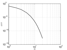
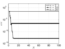
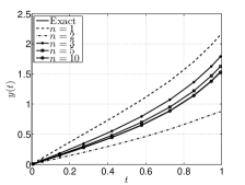
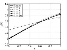
To establish the minimum number of integration points in terms of absolute errors, we note that, from 10 points of integration, we get the same convergence point with more or less iterations (see Fig. 1). It allowed us to conclude that 10 points of integration are sufficient to preserve the convergence of the method. In the next experiment, we take 101010 integration points and numerical solution putting n=1, 2, 3, 5𝑛1235n=1,\ 2,\ 3,\ 5, and 101010 iterations on the successive approximation method. The solutions are compared with the exact solution y​(t)=sin⁑(t)𝑦𝑑𝑑y(t)=\sin(t) as described graphically in Fig. 1. Already, Fig. 1 depicts the decay of the error on L2superscript𝐿2L^{2}-norm of the approximate solution considering a variation in the iterations number n𝑛n, from 111 to 202020, while in Table 1 we present some values associated with these iterations. The results confirm the accuracy of the successive approximation method.

Refer to caption
Refer to caption
Refer to caption
Figure 1: (a) Absolute error (on L2superscript𝐿2L^{2}-norm) of the numerical solution of eq. (19) in relation to number of integration points N𝑁N putting the iterations n=2,10𝑛210n=2,10, 202020, and using semi-log scale; (b) comparison of numerical solution, and exact solution, in 101010 integration points; (c) absolute error (on L2superscript𝐿2L^{2}-norm) of the numerical solution of eq. (19) on iterations number n𝑛n from 111 to 202020 using log-log scale.
Iteration (n) Error in the L2superscript𝐿2L^{2}-norm (err)
1 0.139055224218022
2 0.28090214152532 e-01
3 0.7514001013338 e-02
4 0.1557774788458 e-02
5 0.417391135550 e-03
6 0.86414955296 e-04
10 0.265922221 e-06
12 0.14751583 e-07
15 0.219260 e-09
20 0.174 e-12
Table 1: Error in the L2superscript𝐿2L^{2}-norm of the approximate solution with respect to eq. (18) for the iterations n=1,2,…,20𝑛12…20n=1,2,\ldots,20.

Example 2

Consider the nonlinear functional integral equation:

y​(t)=1t+1​log⁑(∫01(t​x)​arctan⁑(y​(x))​𝑑xβˆ’t3+exp⁑(βˆ’tβˆ’1))+tan⁑(t)+1,𝑦𝑑1𝑑1superscriptsubscript01𝑑π‘₯𝑦π‘₯differential-dπ‘₯𝑑3𝑑1𝑑1y(t)=\frac{1}{t+1}\log\left(\int_{0}^{1}(tx)\arctan(y(x))\,dx-\frac{t}{3}+\exp(-t-1)\right)+\tan(t)+1, (19)

with t∈[0,1]𝑑01t\in[0,1] and exact solution y​(t)=tan⁑(t)𝑦𝑑𝑑y(t)=\tan(t). Consider k​(t,x)=t​xπ‘˜π‘‘π‘₯𝑑π‘₯k(t,x)=tx and

f​(t,z)=1t+1​log⁑(zβˆ’t3+exp⁑(βˆ’tβˆ’1))+tan⁑(t)+1.𝑓𝑑𝑧1𝑑1𝑧𝑑3𝑑1𝑑1f(t,z)=\frac{1}{t+1}\log\left(z-\frac{t}{3}+\exp(-t-1)\right)+\tan(t)+1.

In this example, the hypotheses from Theorem 2.4 are also easily checked.

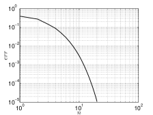
Similar to the previous experiment, in Figs. 2 we plot the approximate solutions of eq. (19) and the error associated with L2superscript𝐿2L^{2}-norm. The numerical solution has a good agreement with the exact solution. In Table 2 we exhibit again some numerical results of this error on L2superscript𝐿2L^{2}-norm.

Refer to caption
Refer to caption
Refer to caption
Figure 2: (a) Absolute error (on L2superscript𝐿2L^{2}-norm) of the numerical solution of eq. (19) in relation to number of integration points N𝑁N putting the iterations n=2,10𝑛210n=2,10, 202020, and using semi-log scale; (b) comparison of numerical solution, and exact solution, in 101010 integration points; (c) absolute error (on L2superscript𝐿2L^{2}-norm) of the numerical solution of eq.(19) on iterations number n𝑛n from 111 to 202020 using log-log scale.
Iteration (n) Error in the L2superscript𝐿2L^{2}-norm (err)
1 0.394366600397979
2 0.276308698116164
3 0.146122318109685
4 0.881455213962e-1
5 0.489253352732e-1
6 0.283969210188e-1
10 0.2994640228e-2
12 0.97457513e-3
15 0.18100617e-3
20 0.109484e-4
Table 2: Error in the L2superscript𝐿2L^{2}-norm of the approximate solution with respect to eq. (19) for the iterations n=1,2,…,20𝑛12…20n=1,2,\ldots,20.

5 Conclusion

In this paper we expand the results of Emannuele [7] in the space Lp​([a,b])superscriptπΏπ‘π‘Žπ‘L^{p}([a,b]) for nonlinear integral equations through of Theorem 2.4. We illustrate the guarantee of existence and uniqueness on the method of successive approximations considering Chebyshev quadrature. The computed errors for the exact solution and the iterated solution present acceptable results.

Acknowledgements

This work was supported by CNPq (grants 441489/2014-1).

References

References

  • [1] K. Atkinson and W. Han. Theoretical Numerical Analysis: A Functional Analysis Framework. Texts in Applied Mathematics. Springer New York, 2001.
  • [2] J. BanaΕ›, Z. Knap. Integrable solutions of a functional-integral equation, Rev. Mat. Univ. Complut. Madrid, 2(1): 31-38, 1989.
  • [3] A. Bielecki. Une remarque sur la mΓ©thode de Banach-Cacciopoli-Tikhonov dans la thΓ©orie des equations diffΓ©rentielles ordinaires, Bull. Acad. Polon. Sci. SΓ©r. Sci. Math. Phys. Astr., 4 (5): 261-264, 1956.
  • [4] A. Bielecki. Une remarque sur l’application de la mΓ©thod de Banach-Cacciopoli-Tikhonov dans la thΓ©orie de l’équation s=f​(x,y,z,p,q)𝑠𝑓π‘₯π‘¦π‘§π‘π‘žs=f(x,y,z,p,q), Bull. Acad. Polon. Sci. SΓ©r. Sci. Math. Phys. Astr., 4: 265-268, 1956.
  • [5] D. G. Figueiredo, C. P. Gupta. On the variational method for the existence of solutions of nonlinear equations of Hammerstein type. Proc. Amer. Math. Soc., 40: 470-476, 1973.
  • [6] G. Emmanuele. About the existence of integrable solutions of a functional-integral equation, Rev. Mat. Univ. Complut. Madrid, 4(1): 65-69, 1991.
  • [7] G. Emmanuele. Integrable solutions of a functional-integral equation, J. Integral Eqns. and Appl., 4 (1): 89-94, 1992.
  • [8] I. A. Ibrahim. On the existence of solutions of functional integral equation of Urysohn type, Comput. Math. Appl., 57 (10), 1609-1614, 2009.
  • [9] A. Karoui. On the existence of continuous solutions of nonlinear integral equations, Appl. Math. Lett., 18(3): 299-305, 2005.
  • [10] A. Karoui, A. Jawahdou. Existence and approximate Lpsuperscript𝐿𝑝L^{p} and continuous solutions of nonlinear integral equations of the Hammerstein and Volterra types, Appl. Math. Comput., 216 (7): 2077-2091, 2010.
  • [11] M. Kwarpisz. Bielecki’s Method, Existence and Uniqueness Results for Volterra Integral Equations in Lp Spaces, Journal of Mathematics Analysis and Applications, 154 (2): 403-416, 1991.
  • [12] M. Nadir, B. Gagui. A numerical approximation for solutions of Hammerstein integral equations in Lp spaces, SΓ£o Paulo Journal of Mathematical Sciences, 8(1): 23-31, 2014.
  • [13] R. Piessens and M. Branders. Numerical solution of integral equations of mathematical physics, using Chebyshev polynomials, J. Comput. Phys, 21 (2): 178-196, 1976.
  • [14] E. Zeidler. Nonlinear Functional Analysis and its Applications I.(Fixed Point Theorems. Springer-Verlag, New York, 1986.

Appendix A
Chebyshev polynomial method

In this section we apply Chebyshev polynomial method (see [13]) for solving one dimensional functional-integral equation (2). We employ Chebyshev polynomial method of the first kind to approximate functions on the interval [a,b]π‘Žπ‘[a,b]. Firstly, we start with some basic definitions.

Definition 5.1.

Chebyshev polynomials of degree n𝑛n are defined as:

Tn​(x)={cos⁑(n​arccos⁑x),if ​|x|≀1,cosh⁑(n​arcosh⁑x),if ​xβ‰₯1,(βˆ’1)n​cosh⁑(n​arcosh⁑(βˆ’x)),if ​xβ‰€βˆ’1.subscript𝑇𝑛π‘₯cases𝑛π‘₯ifΒ π‘₯1𝑛arcoshπ‘₯ifΒ π‘₯1superscript1𝑛𝑛arcoshπ‘₯ifΒ π‘₯1{\displaystyle T_{n}(x)={\begin{cases}\cos{\big{(}}n\arccos x{\big{)}},&{\text{if }}|x|\leq 1,\\ \cosh{\big{(}}n\operatorname{arcosh}x{\big{)}},&{\text{if }}x\geq 1,\\ (-1)^{n}\cosh{\big{(}}n\operatorname{arcosh}(-x){\big{)}},&{\text{if }}x\leq-1.\end{cases}}} (20)

In addition, these polynomials satisfy the following relations:

Tn​(cos⁑θ)=cos⁑n​θ,n=0,1,2,…formulae-sequencesubscriptπ‘‡π‘›πœƒπ‘›πœƒπ‘›012…\displaystyle T_{n}(\cos\theta)=\cos n\theta,\quad n=0,1,2,\ldots

and

βˆ«βˆ’11Tn​(x)​Tm​(x)​d​x1βˆ’x2={0,nβ‰ m,Ο€,n=m=0,Ο€2,n=mβ‰ 0.superscriptsubscript11subscript𝑇𝑛π‘₯subscriptπ‘‡π‘šπ‘₯𝑑π‘₯1superscriptπ‘₯2cases0π‘›π‘šπœ‹π‘›π‘š0πœ‹2π‘›π‘š0{\displaystyle\int_{-1}^{1}\,{\frac{T_{n}(x)T_{m}(x)dx}{\sqrt{1-x^{2}}}}={\begin{cases}0,&n\neq m,\\ \pi,&n=m=0,\\ {\dfrac{\pi}{2},}&n=m\neq 0.\end{cases}}}
Remark 5.1.

The set of Chebyshev polynomials form an orthogonal basis in L2​([a,b])superscript𝐿2π‘Žπ‘L^{2}([a,b]), so that a function f∈L2​([a,b])𝑓superscript𝐿2π‘Žπ‘f\in L^{2}([a,b]) can be approximated via expansion as follows:

f​(x)β‰ˆβˆ‘n=0Man​Tn​(2bβˆ’a​xβˆ’b+abβˆ’a),x∈[a,b],formulae-sequence𝑓π‘₯superscriptsubscript𝑛0𝑀subscriptπ‘Žπ‘›subscript𝑇𝑛2π‘π‘Žπ‘₯π‘π‘Žπ‘π‘Žπ‘₯π‘Žπ‘\displaystyle f(x)\approx\sum_{n=0}^{M}a_{n}T_{n}\left(\frac{2}{b-a}x-\frac{b+a}{b-a}\right),\quad x\in[a,b], (21)

such that

an=2π​dkβ€‹βˆ«βˆ’1+1Tn​(x)​f​(bβˆ’a2​xβˆ’b+a2)1βˆ’x2​𝑑x,dk={2,n=0,1,n>1.formulae-sequencesubscriptπ‘Žπ‘›2πœ‹subscriptπ‘‘π‘˜superscriptsubscript11subscript𝑇𝑛π‘₯π‘“π‘π‘Ž2π‘₯π‘π‘Ž21superscriptπ‘₯2differential-dπ‘₯subscriptπ‘‘π‘˜cases2𝑛01𝑛1a_{n}=\displaystyle\frac{2}{\pi d_{k}}\int_{-1}^{+1}{\frac{T_{n}(x)f(\frac{b-a}{2}x-\frac{b+a}{2})}{\sqrt{1-x^{2}}}}\,dx,\quad d_{k}={\begin{cases}2,&n=0,\\ 1,&n>1.\end{cases}} (22)

We estimate the unknown function y​(t)𝑦𝑑y(t) with the Chebyshev polynomials as

y​(t)β‰ˆyM​(t)=βˆ‘n=0Mcn​Tn​(t).𝑦𝑑subscript𝑦𝑀𝑑superscriptsubscript𝑛0𝑀subscript𝑐𝑛subscript𝑇𝑛𝑑y(t)\approx y_{M}(t)=\sum_{n=0}^{M}c_{n}T_{n}(t). (23)

The unknown coefficients cnsubscript𝑐𝑛c_{n} are determined by selecting collocation points {ti}i=0Msuperscriptsubscriptsubscript𝑑𝑖𝑖0𝑀\{t_{i}\}_{i=0}^{M}, where

ti=bβˆ’a2​xiβˆ’b+a2,xi=c​o​s​(i​πM).formulae-sequencesubscriptπ‘‘π‘–π‘π‘Ž2subscriptπ‘₯π‘–π‘π‘Ž2subscriptπ‘₯π‘–π‘π‘œπ‘ π‘–πœ‹π‘€\displaystyle t_{i}=\frac{b-a}{2}x_{i}-\frac{b+a}{2},\quad x_{i}=cos\left(\frac{i\pi}{M}\right). (24)

The collocation method solves the nonlinear integral equation (2) using approximation (23) through the equations:

yM​(ti)=f​(ti,∫abk​(ti,s)​g​(s,yM​(s))​𝑑s)0≀i≀M.formulae-sequencesubscript𝑦𝑀subscript𝑑𝑖𝑓subscript𝑑𝑖superscriptsubscriptπ‘Žπ‘π‘˜subscript𝑑𝑖𝑠𝑔𝑠subscript𝑦𝑀𝑠differential-d𝑠0𝑖𝑀y_{M}(t_{i})=f\left(t_{i},\int_{a}^{b}k(t_{i},s)g(s,y_{M}(s))ds\right)\qquad 0\leq i\leq M. (25)

Now, by substituting the expression (22) into (25), we get the following system:

βˆ‘n=0Mcn​Tn​(ti)=f​(ti,∫abk​(ti,s)​g​(s,βˆ‘n=0Mcn​Tn​(s))​𝑑s),0≀i≀M,formulae-sequencesuperscriptsubscript𝑛0𝑀subscript𝑐𝑛subscript𝑇𝑛subscript𝑑𝑖𝑓subscript𝑑𝑖superscriptsubscriptπ‘Žπ‘π‘˜subscript𝑑𝑖𝑠𝑔𝑠superscriptsubscript𝑛0𝑀subscript𝑐𝑛subscript𝑇𝑛𝑠differential-d𝑠0𝑖𝑀\sum_{n=0}^{M}c_{n}T_{n}(t_{i})=f\left(t_{i},\int_{a}^{b}k(t_{i},s)g\left(s,\sum_{n=0}^{M}c_{n}T_{n}(s)\right)ds\right),\qquad 0\leq i\leq M, (26)

which in matrix form can be written in terms of the vector 𝒄=[c0,c1,…,cM]T𝒄superscriptsubscript𝑐0subscript𝑐1…subscript𝑐𝑀𝑇\boldsymbol{c}=[c_{0},c_{1},\ldots,c_{M}]^{T} as

𝑻​𝒄=𝑭​(𝒄),𝑻𝒄𝑭𝒄\boldsymbol{T}\boldsymbol{c}=\boldsymbol{F}(\boldsymbol{c}), (27)

with

𝑭​(𝒄)=[F0​(𝒄),…,Fn​(𝒄)]T,𝑭𝒄superscriptsubscript𝐹0𝒄…subscript𝐹𝑛𝒄𝑇\boldsymbol{F}(\boldsymbol{c})=\left[F_{0}(\boldsymbol{c}),\ldots,F_{n}(\boldsymbol{c})\right]^{T},

such that

Fj​(𝒄)=∫abk​(tj,s)​g​(s,βˆ‘n=0Mcn​Tn​(s))​𝑑x,0≀j≀M,formulae-sequencesubscript𝐹𝑗𝒄superscriptsubscriptπ‘Žπ‘π‘˜subscript𝑑𝑗𝑠𝑔𝑠superscriptsubscript𝑛0𝑀subscript𝑐𝑛subscript𝑇𝑛𝑠differential-dπ‘₯0𝑗𝑀F_{j}(\boldsymbol{c})=\int_{a}^{b}k\left(t_{j},s\right)g\left(s,\sum_{n=0}^{M}c_{n}T_{n}(s)\right)\,dx,\quad 0\leq j\leq M,

and

Ti,j=Tj​(ti),0≀i,j≀M.formulae-sequencesubscript𝑇𝑖𝑗subscript𝑇𝑗subscript𝑑𝑖formulae-sequence0𝑖𝑗𝑀T_{i,j}=T_{j}(t_{i}),\quad 0\leq i,j\leq M. (28)

This iterative process can be solved using Picard iteration method due to its nonlinearity. In this way, for each iteration we solve a linear problem:

𝒄(k+1)=π‘»βˆ’1​𝑭​(𝒄(k)),0≀k<km​a​x,formulae-sequencesuperscriptπ’„π‘˜1superscript𝑻1𝑭superscriptπ’„π‘˜0π‘˜subscriptπ‘˜π‘šπ‘Žπ‘₯\boldsymbol{c}^{(k+1)}=\boldsymbol{T}^{-1}\boldsymbol{F}(\boldsymbol{c}^{(k)}),\quad 0\leq k<k_{max}, (29)

with 𝒄(k)=[c0(k),c1(k),…,cM(k)]Tsuperscriptπ’„π‘˜superscriptsuperscriptsubscript𝑐0π‘˜superscriptsubscript𝑐1π‘˜β€¦superscriptsubscriptπ‘π‘€π‘˜π‘‡\boldsymbol{c}^{(k)}=[c_{0}^{(k)},c_{1}^{(k)},\ldots,c_{M}^{(k)}]^{T}. The iterative process is stopped until the following stopping criterion is satisfied:

‖𝒄(k+1)βˆ’π’„(k)β€–p<t​o​l.subscriptnormsuperscriptπ’„π‘˜1superscriptπ’„π‘˜π‘π‘‘π‘œπ‘™\|\boldsymbol{c}^{(k+1)}-\boldsymbol{c}^{(k)}\|_{p}<tol. (30)