Sparse Regularization via Convex Analysis

Ivan Selesnick Department of Electrical and Computer Engineering, Tandon School of Engineering, New York University, New York, USA. Email: selesi@nyu.edu. This work was supported by NSF under grant CCF-1525398 and ONR under grant N00014-15-1-2314. Software is available online:
       https://codeocean.com/2017/06/21/gmc-sparse-regularization (Matlab)
       https://codeocean.com/2017/06/22/gmc-sparse-regularization (Python)
       http://ieeexplore.ieee.org/document/7938377/media (Matlab)

I. Selesnick, “Sparse Regularization via Convex Analysis” in IEEE Transactions on Signal Processing, vol. 65, no. 17, pp. 4481-4494, Sept. 2017. doi: 10.1109/TSP.2017.2711501
Abstract

Sparse approximate solutions to linear equations are classically obtained via L1 norm regularized least squares, but this method often underestimates the true solution. As an alternative to the L1 norm, this paper proposes a class of non-convex penalty functions that maintain the convexity of the least squares cost function to be minimized, and avoids the systematic underestimation characteristic of L1 norm regularization. The proposed penalty function is a multivariate generalization of the minimax-concave (MC) penalty. It is defined in terms of a new multivariate generalization of the Huber function, which in turn is defined via infimal convolution. The proposed sparse-regularized least squares cost function can be minimized by proximal algorithms comprising simple computations.

1 Introduction

Numerous signal and image processing techniques build upon sparse approximation [59]. A sparse approximate solution to a system of linear equations (y=Ax𝑦𝐴𝑥y=Ax) can often be obtained via convex optimization. The usual technique is to minimize the regularized linear least squares cost function J:N:𝐽superscript𝑁J\colon\mathbb{R}^{N}\to\mathbb{R},

J(x)=12yAx22+λx1,λ>0.formulae-sequence𝐽𝑥12superscriptsubscriptdelimited-∥∥𝑦𝐴𝑥22𝜆subscriptdelimited-∥∥𝑥1𝜆0J(x)=\frac{1}{2}\lVert y-Ax\rVert_{2}^{2}+{\lambda}\lVert x\rVert_{1},\quad{\lambda}>0. (1)

The 1subscript1\ell_{1} norm is classically used as a regularizer here, since among convex regularizers it induces sparsity most effectively [9]. But this formulation tends to underestimate high-amplitude components of xN𝑥superscript𝑁x\in\mathbb{R}^{N}. Non-convex sparsity-inducing regularizers are also widely used (leading to more accurate estimation of high-amplitude components), but then the cost function is generally non-convex and has extraneous suboptimal local minimizers [43].

This paper proposes a class of non-convex penalties for sparse-regularized linear least squares that generalizes the 1subscript1\ell_{1} norm and maintains the convexity of the least squares cost function to be minimized. That is, we consider the cost function F:N:𝐹superscript𝑁F\colon\mathbb{R}^{N}\to\mathbb{R}

F(x)=12yAx22+λψB(x),λ>0formulae-sequence𝐹𝑥12superscriptsubscriptdelimited-∥∥𝑦𝐴𝑥22𝜆subscript𝜓𝐵𝑥𝜆0F(x)=\frac{1}{2}\lVert y-Ax\rVert_{2}^{2}+{\lambda}\,\psi_{B}(x),\quad{\lambda}>0 (2)

and we propose a new non-convex penalty ψB:N:subscript𝜓𝐵superscript𝑁\psi_{B}\colon\mathbb{R}^{N}\to\mathbb{R} that makes F𝐹F convex. The penalty ψBsubscript𝜓𝐵\psi_{B} is parameterized by a matrix B𝐵B, and the convexity of F𝐹F depends on B𝐵B being suitably prescribed. In fact, the choice of B𝐵B will depend on A𝐴A.

The matrix (linear operator) A𝐴A may be arbitrary (i.e., injective, surjective, both, or neither). In contrast to the 1subscript1\ell_{1} norm, the new approach does not systematically underestimate high-amplitude components of sparse vectors. Since the proposed formulation is convex, the cost function has no suboptimal local minimizers.

The new class of non-convex penalties is defined using tools of convex analysis. In particular, infimal convolution is used to define a new multivariate generalization of the Huber function. In turn, the generalized Huber function is used to define the proposed non-convex penalty, which can be considered a multivariate generalization of the minimax-concave (MC) penalty. Even though the generalized MC (GMC) penalty is non-convex, it is easy to prescribe this penalty so as to maintain the convexity of the cost function to be minimized.

The proposed convex cost functions can be minimized using proximal algorithms, comprising simple computations. In particular, the minimization problem can be cast as a kind of saddle-point problem for which the forward-backward splitting algorithm is applicable. The main computational steps of the algorithm are the operators A𝐴A, A𝖳superscript𝐴𝖳A^{\mathsf{T}}, and soft thresholding. The implementation is thus ‘matrix-free’ in that it involves the operators A𝐴A and A𝖳superscript𝐴𝖳A^{\mathsf{T}}, but does not access or modify the entries of A𝐴A. Hence, the algorithm can leverage efficient implementations of A𝐴A and its transpose.

We remark that while the proposed GMC penalty is non-separable, we do not advocate non-separability in and of itself as a desirable property of a sparsity-inducing penalty. But in many cases (depending on A𝐴A), non-separability is simply a requirement of a non-convex penalty designed so as to maintain convexity of the cost function F𝐹F to be minimized. If A𝖳Asuperscript𝐴𝖳𝐴A^{\mathsf{T}}\!A is singular (and none of its eigenvectors are standard basis vectors), then a separable penalty that maintains the convexity of the cost function F𝐹F must, in fact, be a convex penalty [55]. This leads us back to the 1subscript1\ell_{1} norm. Thus, to improve upon the 1subscript1\ell_{1} norm, the penalty must be non-separable.

This paper is organized as follows. Section 2 sets notation and recalls definitions of convex analysis. Section 3 recalls the (scalar) Huber function, the (scalar) MC penalty, and how they arise in the formulation of threshold functions (instances of proximity operators). The subsequent sections generalize these concepts to the multivariate case. In Section 4, we define a multivariate version of the Huber function. In Section 5, we define a multivariate version of the MC penalty. In Section 6, we show how to set the GMC penalty to maintain convexity of the least squares cost function. Section 7 presents a proximal algorithm to minimize this type of cost function. Section 8 presents examples wherein the GMC penalty is used for signal denoising and approximation.

Elements of this work were presented in Ref. [49].

1.1 Related work

Many prior works have proposed non-convex penalties that strongly promote sparsity or describe algorithms for solving the sparse-regularized linear least squares problem, e.g., [13, 11, 43, 39, 38, 15, 25, 31, 19, 47, 66, 16, 30, 58, 64]. However, most of these papers (i) use separable (additive) penalties or (ii) do not seek to maintain convexity of the cost function. Non-separable non-convex penalties are proposed in Refs. [60, 63], but they are not designed to maintain cost function convexity. The development of convexity-preserving non-convex penalties was pioneered by Blake, Zisserman, and Nikolova [7, 41, 44, 43, 42], and further developed in [6, 17, 23, 32, 36, 37, 45, 54, 56]. But these are separable penalties, and as such they are fundamentally limited. Specifically, if A𝖳Asuperscript𝐴𝖳𝐴A^{\mathsf{T}}\!A is singular, then a separable penalty constrained to maintain cost function convexity can only improve on the 1subscript1\ell_{1} norm to a very limited extent [55]. Non-convex regularization that maintains cost function convexity was used in [35] in an iterative manner for non-convex optimization, to reduce the likelihood that an algorithm converges to suboptimal local minima.

To overcome the fundamental limitation of separable non-convex penalties, we proposed a bivariate non-separable non-convex penalty that maintains the convexity of the cost function to be minimized [55]. But that penalty is useful for only a narrow class of linear inverse problems. To handle more general problems, we subsequently proposed a multivariate penalty formed by subtracting from the 1subscript1\ell_{1} norm a function comprising the composition of a linear operator and a separable nonlinear function [52]. Technically, this type of multivariate penalty is non-separable, but it still constitutes a rather narrow class of non-separable functions.

Convex analysis tools (especially the Moreau envelope and the Fenchel conjugate) have recently been used in novel ways for sparse regularized least squares [12, 57]. Among other aims, these papers seek the convex envelope of the 0subscript0\ell_{0} pseudo-norm regularized least squares cost function, and derive alternate cost functions that share the same global minimizers but have fewer local minima. In these approaches, algorithms are less likely to converge to suboptimal local minima (the global minimizer might still be difficult to calculate).

For the special case where A𝖳Asuperscript𝐴𝖳𝐴A^{\mathsf{T}}\!A is diagonal, the proposed GMC penalty is closely related to the ‘continuous exact 0subscript0\ell_{0}’ (CEL0) penalty introduced in [57]. In [57] it is observed that if A𝖳Asuperscript𝐴𝖳𝐴A^{\mathsf{T}}\!A is diagonal, then the global minimizers of the 0subscript0\ell_{0} regularized problem coincides with that of a convex function defined using the CEL0 penalty. Although the diagonal case is simpler than the non-diagonal case (a non-convex penalty can be readily constructed to maintain cost function convexity [54]), the connection to the 0subscript0\ell_{0} problem is enlightening.

In other related work, we use convex analysis concepts (specifically, the Moreau envelope) for the problem of total variation (TV) denoising [51]. In particular, we prescribe a non-convex TV penalty that preserves the convexity of the TV denoising cost function to be minimized. The approach of Ref. [51] generalizes standard TV denoising so as to more accurately estimate jump discontinuities.

2 Notation

The 1subscript1\ell_{1}, 2subscript2\ell_{2}, and subscript\ell_{\infty} norms of xN𝑥superscript𝑁x\in\mathbb{R}^{N} are defined x1=n|xn|subscriptdelimited-∥∥𝑥1subscript𝑛subscript𝑥𝑛\lVert x\rVert_{1}=\sum_{n}\lvert x_{n}\rvert, x2=(n|xn|2)1/2subscriptdelimited-∥∥𝑥2superscriptsubscript𝑛superscriptsubscript𝑥𝑛212\lVert x\rVert_{2}=\bigl{(}\sum_{n}\lvert x_{n}\rvert^{2}\bigr{)}^{1/2}, and x=maxn|xn|subscriptdelimited-∥∥𝑥subscript𝑛subscript𝑥𝑛\lVert x\rVert_{\infty}=\max_{n}\lvert x_{n}\rvert. If AM×N𝐴superscript𝑀𝑁A\in\mathbb{R}^{M\times N}, then component n𝑛n of Ax𝐴𝑥Ax is denoted [Ax]nsubscriptdelimited-[]𝐴𝑥𝑛[Ax]_{n}. If the matrix AB𝐴𝐵A-B is positive semidefinite, we write BAprecedes-or-equals𝐵𝐴B\preccurlyeq A. The matrix 2-norm of matrix A𝐴A is denoted A2subscriptdelimited-∥∥𝐴2\lVert A\rVert_{2} and its value is the square root of the maximum eigenvalue of A𝖳Asuperscript𝐴𝖳𝐴A^{\mathsf{T}}\!A. We have Ax2A2x2subscriptdelimited-∥∥𝐴𝑥2subscriptdelimited-∥∥𝐴2subscriptdelimited-∥∥𝑥2\lVert Ax\rVert_{2}\leqslant\lVert A\rVert_{2}\lVert x\rVert_{2} for all xN𝑥superscript𝑁x\in\mathbb{R}^{N}. If A𝐴A has full row-rank (i.e., AA𝖳𝐴superscript𝐴𝖳AA^{\mathsf{T}} is invertible), then the pseudo-inverse of A𝐴A is given by A+:=A𝖳(AA𝖳)1assignsuperscript𝐴superscript𝐴𝖳superscript𝐴superscript𝐴𝖳1A^{\mathsf{+}}:=A^{\mathsf{T}}(AA^{\mathsf{T}})^{-1}. We denote the transpose of the pseudo-inverse of A𝐴A as A+𝖳superscript𝐴𝖳A^{\mathsf{+T}}, i.e., A+𝖳:=(A+)𝖳assignsuperscript𝐴𝖳superscriptsuperscript𝐴𝖳A^{\mathsf{+T}}:=(A^{\mathsf{+}})^{\mathsf{T}}. If A𝐴A has full row-rank, then A+𝖳=(AA𝖳)1Asuperscript𝐴𝖳superscript𝐴superscript𝐴𝖳1𝐴A^{\mathsf{+T}}=(AA^{\mathsf{T}})^{-1}A.

This work uses definitions and notation of convex analysis [4]. The infimal convolution of two functions f𝑓f and g𝑔g from Nsuperscript𝑁\mathbb{R}^{N} to {+}\mathbb{R}\cup\{+\infty\} is given by

(fg)(x)=infvN{f(v)+g(xv)}.𝑓𝑔𝑥subscriptinfimum𝑣superscript𝑁𝑓𝑣𝑔𝑥𝑣(f\mbox{\footnotesize$\;\square\;$}g)(x)=\inf_{v\in\mathbb{R}^{N}}\bigl{\{}f(v)+g(x-v)\big{\}}. (3)

The Moreau envelope of the function f:N:𝑓superscript𝑁f\colon\mathbb{R}^{N}\to\mathbb{R} is given by

f𝖬(x)=infvN{f(v)+12xv22}.superscript𝑓𝖬𝑥subscriptinfimum𝑣superscript𝑁𝑓𝑣12superscriptsubscriptdelimited-∥∥𝑥𝑣22f^{\mathsf{M}}(x)=\inf_{v\in\mathbb{R}^{N}}\bigl{\{}f(v)+\tfrac{1}{2}\lVert x-v\rVert_{2}^{2}\bigr{\}}. (4)

In the notation of infimal convolution, we have

f𝖬=f1222.superscript𝑓𝖬𝑓12superscriptsubscriptdelimited-∥∥22f^{\mathsf{M}}=f\mbox{\footnotesize$\;\square\;$}\tfrac{1}{2}\lVert{\,\cdot\,}\rVert_{2}^{2}. (5)

The set of proper lower semicontinuous (lsc) convex functions from Nsuperscript𝑁\mathbb{R}^{N} to {+}\mathbb{R}\cup\{+\infty\} is denoted Γ0(N)subscriptΓ0superscript𝑁\Gamma_{0}(\mathbb{R}^{N}).

If the function f𝑓f is defined as the composition f(x)=h(g(x))𝑓𝑥𝑔𝑥f(x)=h(g(x)), then we write f=hg𝑓𝑔f=h\mathbin{\circ}g.

The soft threshold function soft::soft\operatorname{soft}\colon\mathbb{R}\to\mathbb{R} with threshold parameter λ0𝜆0{\lambda}\geqslant 0 is defined as

soft(y;λ):={0,|y|λ(|y|λ)sign(y),|y|λ.assignsoft𝑦𝜆cases0𝑦𝜆𝑦𝜆sign𝑦𝑦𝜆\operatorname{soft}(y;{\lambda}):=\\ \begin{cases}0,\quad&\lvert y\rvert\leqslant{\lambda}\\ (\lvert y\rvert-{\lambda})\operatorname{sign}(y),\quad&\lvert y\rvert\geqslant{\lambda}.\end{cases} (6)
Refer to caption
Figure 1: The Huber function.

3 Scalar Penalties

We recall the definition of the Huber function [33].

Definition 1.

The Huber function s::𝑠s\colon\mathbb{R}\to\mathbb{R} is defined as

s(x):={12x2,|x|1|x|12,|x|1,assign𝑠𝑥cases12superscript𝑥2𝑥1𝑥12𝑥1s(x):=\begin{cases}\tfrac{1}{2}x^{2},\quad&\lvert x\rvert\leqslant 1\\ \lvert x\rvert-\frac{1}{2},&\lvert x\rvert\geqslant 1,\end{cases} (7)

as illustrated in Fig. 1.

Proposition 1.

The Huber function can be written as

s(x)=minv{|v|+12(xv)2}.𝑠𝑥subscript𝑣𝑣12superscript𝑥𝑣2s(x)=\min_{v\in\mathbb{R}}\{\lvert v\rvert+\tfrac{1}{2}(x-v)^{2}\}. (8)

In the notation of infimal convolution, we have equivalently

s=||12()2.𝑠12superscript2s=\lvert{\,\cdot\,}\rvert\mbox{\footnotesize$\;\square\;$}\tfrac{1}{2}({\,\cdot\,})^{2}. (9)

And in the notation of the Moreau envelope, we have equivalently s=||𝖬𝑠superscript𝖬s=\lvert{\,\cdot\,}\rvert^{\mathsf{M}}.

The Huber function is a standard example of the Moreau envelope. For example, see Sec. 3.1 of Ref. [46] and [20]. We note here that, given x𝑥x\in\mathbb{R}, the minimum in (8) is achieved for v𝑣v equal to 00, x1𝑥1x-1, or x+1𝑥1x+1, i.e.,

s(x)=minv{0,x1,x+1}{|v|+12(xv)2}.𝑠𝑥subscript𝑣0𝑥1𝑥1𝑣12superscript𝑥𝑣2s(x)=\min_{v\in\{0,\,x-1,\,x+1\}}\{\lvert v\rvert+\tfrac{1}{2}(x-v)^{2}\}. (10)

Consequently, the Huber function can be expressed as

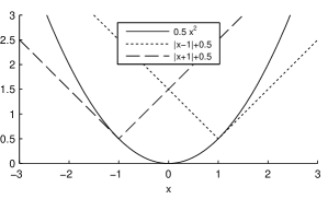
s(x)=min{12x2,|x1|+12,|x+1|+12}𝑠𝑥12superscript𝑥2𝑥112𝑥112s(x)=\min\bigl{\{}\tfrac{1}{2}x^{2},\ \lvert x-1\rvert+\tfrac{1}{2},\ \lvert x+1\rvert+\tfrac{1}{2}\bigr{\}} (11)

as illustrated in Fig. 2.

Refer to caption
Figure 2: The Huber function as the pointwise minimum of three functions.

We now consider the scalar penalty function illustrated in Fig. 3. This is the minimax-concave (MC) penalty [65]; see also [28, 6, 5].

Definition 2.

The minimax-concave (MC) penalty function ϕ::italic-ϕ\phi\colon\mathbb{R}\to\mathbb{R} is defined as

ϕ(x):={|x|12x2,|x|112,|x|1,assignitalic-ϕ𝑥cases𝑥12superscript𝑥2𝑥112𝑥1\phi(x):=\begin{cases}\lvert x\rvert-\frac{1}{2}x^{2},\ &\lvert x\rvert\leqslant 1\\ \frac{1}{2},&\lvert x\rvert\geqslant 1,\end{cases} (12)

as illustrated in Fig. 3.

The MC penalty can be expressed as

ϕ(x)=|x|s(x)italic-ϕ𝑥𝑥𝑠𝑥\phi(x)=\lvert x\rvert-s(x) (13)

where s𝑠s is the Huber function. This representation of the MC penalty will be used in Sec. 5 to generalize the MC penalty to the multivariate case.

Refer to caption
Figure 3: The MC penalty function.

3.1 Scaled functions

It will be convenient to define scaled versions of the Huber function and MC penalty.

Definition 3.

Let b𝑏b\in\mathbb{R}. The scaled Huber function sb::subscript𝑠𝑏s_{b}\colon\mathbb{R}\to\mathbb{R} is defined as

sb(x):=s(b2x)/b2,b0.formulae-sequenceassignsubscript𝑠𝑏𝑥𝑠superscript𝑏2𝑥superscript𝑏2𝑏0s_{b}(x):=s({b}^{2}x)/{b}^{2},\ \ b\neq 0. (14)

For b=0𝑏0b=0, the function is defined as

s0(x):=0.assignsubscript𝑠0𝑥0s_{0}(x):=0. (15)

Hence, for b0𝑏0b\neq 0, the scaled Huber function is given by

sb(x)={12b2x2,|x|1/b2|x|12b2,|x|1/b2.subscript𝑠𝑏𝑥cases12superscript𝑏2superscript𝑥2𝑥1superscript𝑏2𝑥12superscript𝑏2𝑥1superscript𝑏2s_{b}(x)=\begin{cases}\frac{1}{2}{b}^{2}x^{2},\quad&\lvert x\rvert\leqslant 1/{b}^{2}\\ \lvert x\rvert-\frac{1}{2{b}^{2}},&\lvert x\rvert\geqslant 1/{b}^{2}.\end{cases} (16)

The scaled Huber function sbsubscript𝑠𝑏s_{b} is shown in Fig. 4 for several values of the scaling parameter b𝑏b. Note that

0sb(x)|x|,x,formulae-sequence0subscript𝑠𝑏𝑥𝑥for-all𝑥0\leqslant s_{b}(x)\leqslant\lvert x\rvert,\quad\forall x\in\mathbb{R}, (17)

and

limbsb(x)subscript𝑏subscript𝑠𝑏𝑥\displaystyle\lim_{{b}\to\infty}s_{b}(x) =|x|absent𝑥\displaystyle=\lvert x\rvert (18)
limb0sb(x)subscript𝑏0subscript𝑠𝑏𝑥\displaystyle\lim_{{b}\to 0}s_{b}(x) =0.absent0\displaystyle=0. (19)

Incidentally, we use b2superscript𝑏2b^{2} in definition (14) rather than b𝑏b, so as to parallel the generalized Huber function to be defined in Sec. 4.

Proposition 2.

Let b𝑏b\in\mathbb{R}. The scaled Huber function can be written as

sb(x)=minv{|v|+12b2(xv)2}.subscript𝑠𝑏𝑥subscript𝑣𝑣12superscript𝑏2superscript𝑥𝑣2s_{b}(x)=\min_{v\in\mathbb{R}}\{\lvert v\rvert+\tfrac{1}{2}{b}^{2}(x-v)^{2}\}. (20)

In terms of infimal convolution, we have equivalently

sb=||12b2()2.subscript𝑠𝑏12superscript𝑏2superscript2s_{b}=\lvert{\,\cdot\,}\rvert\mbox{\footnotesize$\;\square\;$}\tfrac{1}{2}{b}^{2}({\,\cdot\,})^{2}. (21)
Proof.

For b0𝑏0b\neq 0, we have from (14) that

sb(x)subscript𝑠𝑏𝑥\displaystyle s_{b}(x) =minv{|v|+12(b2xv)2}/b2absentsubscript𝑣𝑣12superscriptsuperscript𝑏2𝑥𝑣2superscript𝑏2\displaystyle=\min_{v\in\mathbb{R}}\{\lvert v\rvert+\tfrac{1}{2}({b}^{2}x-v)^{2}\}/{b}^{2}
=minv{|b2v|+12(b2xb2v)2}/b2absentsubscript𝑣superscript𝑏2𝑣12superscriptsuperscript𝑏2𝑥superscript𝑏2𝑣2superscript𝑏2\displaystyle=\min_{v\in\mathbb{R}}\{\lvert{b}^{2}v\rvert+\tfrac{1}{2}({b}^{2}x-{b}^{2}v)^{2}\}/{b}^{2}
=minv{|v|+12b2(xv)2}.absentsubscript𝑣𝑣12superscript𝑏2superscript𝑥𝑣2\displaystyle=\min_{v\in\mathbb{R}}\{\lvert v\rvert+\tfrac{1}{2}{b}^{2}(x-v)^{2}\}.

It follows from ||0=000\lvert{\,\cdot\,}\rvert\mbox{\footnotesize$\;\square\;$}0=0 that (20) holds for b=0𝑏0b=0. ∎

Definition 4.

Let b𝑏b\in\mathbb{R}. The scaled MC penalty function ϕb::subscriptitalic-ϕ𝑏\phi_{b}\colon\mathbb{R}\to\mathbb{R} is defined as

ϕb(x)subscriptitalic-ϕ𝑏𝑥\displaystyle\phi_{b}(x) :=|x|sb(x)assignabsent𝑥subscript𝑠𝑏𝑥\displaystyle:=\lvert x\rvert-s_{b}(x) (22)

where sbsubscript𝑠𝑏s_{b} is the scaled Huber function.

The scaled MC penalty ϕbsubscriptitalic-ϕ𝑏\phi_{b} is shown in Fig. 4 for several values of b𝑏b. Note that ϕ0(x)=|x|subscriptitalic-ϕ0𝑥𝑥\phi_{0}(x)=\lvert x\rvert. For b0𝑏0b\neq 0,

ϕb(x)={|x|12b2x2,|x|1/b212b2,|x|1/b2.subscriptitalic-ϕ𝑏𝑥cases𝑥12superscript𝑏2superscript𝑥2𝑥1superscript𝑏212superscript𝑏2𝑥1superscript𝑏2\phi_{b}(x)=\begin{cases}\lvert x\rvert-\frac{1}{2}{b}^{2}x^{2},\quad&\lvert x\rvert\leqslant 1/{b}^{2}\\ \frac{1}{2{b}^{2}},&\lvert x\rvert\geqslant 1/{b}^{2}.\end{cases} (23)
Refer to caption
Figure 4: Scaled Huber function and MC penalty for several values of the scaling parameter.

3.2 Convexity condition

In the scalar case, the MC penalty corresponds to a type of threshold function. Specifically, the firm threshold function is the proximity operator of the MC penalty, provided that a particular convexity condition is satisfied. Here, we give the convexity condition for the scalar case. We will generalize this condition to the multivariate case in Sec. 6.

Proposition 3.

Let λ>0𝜆0{\lambda}>0 and a𝑎a\in\mathbb{R}. Define f::𝑓f\colon\mathbb{R}\to\mathbb{R},

f(x)=12(yax)2+λϕb(x)𝑓𝑥12superscript𝑦𝑎𝑥2𝜆subscriptitalic-ϕ𝑏𝑥f(x)=\frac{1}{2}(y-ax)^{2}+{\lambda}\,\phi_{b}(x) (24)

where ϕbsubscriptitalic-ϕ𝑏\phi_{b} is the scaled MC penalty (22). If

b2a2/λ,superscript𝑏2superscript𝑎2𝜆{b}^{2}\leqslant a^{2}/{\lambda}, (25)

then f𝑓f is convex.

There are several ways to prove Proposition 3. In anticipation of the multivariate case, we use a technique in the following proof that we later use in the proof of Theorem 1 in Sec. 6.

Proof of Proposition 3.

Using (22), we write f𝑓f as

f(x)𝑓𝑥\displaystyle f(x) =12(yax)2+λ|x|λsb(x)absent12superscript𝑦𝑎𝑥2𝜆𝑥𝜆subscript𝑠𝑏𝑥\displaystyle=\tfrac{1}{2}(y-ax)^{2}+{\lambda}\lvert x\rvert-{\lambda}s_{b}(x)
=g(x)+λ|x|absent𝑔𝑥𝜆𝑥\displaystyle=g(x)+{\lambda}\lvert x\rvert

where sbsubscript𝑠𝑏s_{b} is the scaled Huber function and g::𝑔g\colon\mathbb{R}\to\mathbb{R} is given by

g(x)=12(yax)2λsb(x).𝑔𝑥12superscript𝑦𝑎𝑥2𝜆subscript𝑠𝑏𝑥g(x)=\tfrac{1}{2}(y-ax)^{2}-{\lambda}s_{b}(x). (26)

Since the sum of two convex functions is convex, it is sufficient to show g𝑔g is convex. Using (20), we have

g(x)𝑔𝑥\displaystyle g(x) =12(yax)2λminv{|v|+12b2(xv)2}absent12superscript𝑦𝑎𝑥2𝜆subscript𝑣𝑣12superscript𝑏2superscript𝑥𝑣2\displaystyle=\tfrac{1}{2}(y-ax)^{2}-{\lambda}\min_{v\in\mathbb{R}}\{\lvert v\rvert+\tfrac{1}{2}{b}^{2}(x-v)^{2}\}
=maxv{12(yax)2λ|v|12λb2(xv)2}absentsubscript𝑣12superscript𝑦𝑎𝑥2𝜆𝑣12𝜆superscript𝑏2superscript𝑥𝑣2\displaystyle=\max_{v\in\mathbb{R}}\left\{\tfrac{1}{2}(y-ax)^{2}-{\lambda}\lvert v\rvert-\tfrac{1}{2}{\lambda}{b}^{2}(x-v)^{2}\right\}
=12(a2λb2)x2+maxv{12(y22axy)λ|v|12λb2(v22xv)}.absent12superscript𝑎2𝜆superscript𝑏2superscript𝑥2subscript𝑣12superscript𝑦22𝑎𝑥𝑦𝜆𝑣12𝜆superscript𝑏2superscript𝑣22𝑥𝑣\displaystyle=\tfrac{1}{2}(a^{2}-{\lambda}{b}^{2})x^{2}+\max_{v\in\mathbb{R}}\big{\{}\tfrac{1}{2}(y^{2}-2axy)-{\lambda}\lvert v\rvert-\tfrac{1}{2}{\lambda}{b}^{2}(v^{2}-2xv)\big{\}}.

Note that the expression in the curly braces is affine (hence convex) in x𝑥x. Since the pointwise maximum of a set of convex functions is itself convex, the second term is convex in x𝑥x. Hence, g𝑔g is convex if a2λb20superscript𝑎2𝜆superscript𝑏20a^{2}-{\lambda}{b}^{2}\geqslant 0. ∎

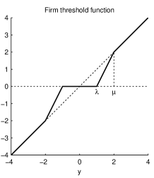
The firm threshold function was defined by Gao and Bruce [29] as a generalization of hard and soft thresholding.
Refer to caption
Figure 5: Firm threshold function.
Definition 5.

Let λ>0𝜆0{\lambda}>0 and μ>λ𝜇𝜆\mu>{\lambda}. The threshold function firm::firm\operatorname{firm}\colon\mathbb{R}\to\mathbb{R} is defined as

firm(y;λ,μ):={0,|y|λμ(|y|λ)/(μλ)sign(y),λ|y|μy,|y|μassignfirm𝑦𝜆𝜇cases0𝑦𝜆𝜇𝑦𝜆𝜇𝜆sign𝑦𝜆𝑦𝜇𝑦𝑦𝜇\operatorname{firm}(y;{\lambda},\mu):=\begin{cases}0,\quad&\lvert y\rvert\leqslant{\lambda}\\ \mu(\lvert y\rvert-{\lambda})/(\mu-{\lambda})\operatorname{sign}(y),\quad&{\lambda}\leqslant\lvert y\rvert\leqslant\mu\\ y,&\lvert y\rvert\geqslant\mu\end{cases} (27)

as illustrated in Fig. 5.

In contrast to the soft threshold function, the firm threshold function does not underestimate large amplitude values, since it equals the identity for large values of its argument. As μλ𝜇𝜆\mu\to{\lambda} or μ𝜇\mu\to\infty, the firm threshold function approaches the hard or soft threshold function, respectively.

We now state the correspondence between the MC penalty and the firm threshold function. When f𝑓f in (24) is convex (i.e., b2a2/λsuperscript𝑏2superscript𝑎2𝜆b^{2}\leqslant a^{2}/{\lambda}), the minimizer of f𝑓f is given by firm thresholding. This is noted in Refs. [28, 65, 64, 5].

Proposition 4.

Let λ>0𝜆0{\lambda}>0, a>0𝑎0a>0, b>0𝑏0b>0, and b2a2/λsuperscript𝑏2superscript𝑎2𝜆b^{2}\leqslant a^{2}/{\lambda}. Let y𝑦y\in\mathbb{R}. Then the minimizer of f𝑓f in (24) is given by firm thresholding, i.e.,

x𝗈𝗉𝗍=firm(y/a;λ/a2,1/b2).superscript𝑥𝗈𝗉𝗍firm𝑦𝑎𝜆superscript𝑎21superscript𝑏2x^{\mathsf{opt}}=\operatorname{firm}(y/a;{\lambda}/a^{2},1/b^{2}). (28)

Hence, the minimizer of the scalar function f𝑓f in (24) is easily obtained via firm thresholding. However, the situation in the multivariate case is more complicated. The aim of this paper is to generalize this process to the multivariate case: to define a multivariate MC penalty generalizing (12), to define a regularized least squares cost function generalizing (24), to generalize the convexity condition (25), and to provide a method to calculate a minimizer.

4 Generalized Huber Function

In this section, we introduce a multivariate generalization of the Huber function. The basic idea is to generalize (20) which expresses the scalar Huber function as an infimal convolution.

Definition 6.

Let BM×N𝐵superscript𝑀𝑁B\in\mathbb{R}^{M\times N}. We define the generalized Huber function SB:N:subscript𝑆𝐵superscript𝑁S_{B}\colon\mathbb{R}^{N}\to\mathbb{R} as

SB(x):=infvN{v1+12B(xv)22}.assignsubscript𝑆𝐵𝑥subscriptinfimum𝑣superscript𝑁subscriptdelimited-∥∥𝑣112superscriptsubscriptdelimited-∥∥𝐵𝑥𝑣22S_{B}(x):=\inf_{v\in\mathbb{R}^{N}}\bigl{\{}\lVert v\rVert_{1}+\tfrac{1}{2}\lVert B(x-v)\rVert_{2}^{2}\bigr{\}}. (29)

In the notation of infimal convolution, we have

SB=112B22.S_{B}=\lVert{\,\cdot\,}\rVert_{1}\mbox{\footnotesize$\;\square\;$}\tfrac{1}{2}\lVert B{\,\cdot\,}\rVert_{2}^{2}. (30)
Proposition 5.

The generalized Huber function SBsubscript𝑆𝐵S_{B} is a proper lower semicontinuous convex function, and the infimal convolution is exact, i.e.,

SB(x)=minvN{v1+12B(xv)22}.subscript𝑆𝐵𝑥subscript𝑣superscript𝑁subscriptdelimited-∥∥𝑣112superscriptsubscriptdelimited-∥∥𝐵𝑥𝑣22S_{B}(x)=\min_{v\in\mathbb{R}^{N}}\bigl{\{}\lVert v\rVert_{1}+\tfrac{1}{2}\lVert B(x-v)\rVert_{2}^{2}\bigr{\}}. (31)
Proof.

Set f=1𝑓subscriptdelimited-∥∥1f=\lVert{\,\cdot\,}\rVert_{1} and g=B22g=\lVert B{\,\cdot\,}\rVert_{2}^{2}. Both f𝑓f and g𝑔g are convex; hence fg𝑓𝑔f\mbox{\footnotesize$\;\square\;$}g is convex by proposition 12.11 in [4]. Since f𝑓f is coercive and g𝑔g is bounded below, and f,gΓ0(N)𝑓𝑔subscriptΓ0superscript𝑁f,g\in\Gamma_{0}(\mathbb{R}^{N}), it follows that fgΓ0(N)𝑓𝑔subscriptΓ0superscript𝑁f\mbox{\footnotesize$\;\square\;$}g\in\Gamma_{0}(\mathbb{R}^{N}) and the infimal convolution is exact (i.e., the infimum is achieved for some v𝑣v) by Proposition 12.14 in [4]. ∎

Note that if C𝖳C=B𝖳Bsuperscript𝐶𝖳𝐶superscript𝐵𝖳𝐵C^{\mathsf{T}}\!C=B^{\mathsf{T}}\!B, then SB(x)=SC(x)subscript𝑆𝐵𝑥subscript𝑆𝐶𝑥S_{B}(x)=S_{C}(x) for all x𝑥x. That is, the generalized Huber function SBsubscript𝑆𝐵S_{B} depends only on B𝖳Bsuperscript𝐵𝖳𝐵B^{\mathsf{T}}\!B, not on B𝐵B itself. Therefore, without loss of generality, we may assume B𝐵B has full row-rank. (If a given matrix B𝐵B does not have full row-rank, then there is another matrix C𝐶C with full row-rank such that C𝖳C=B𝖳Bsuperscript𝐶𝖳𝐶superscript𝐵𝖳𝐵C^{\mathsf{T}}\!C=B^{\mathsf{T}}\!B, yielding the same function SBsubscript𝑆𝐵S_{B}.)

As expected, the generalized Huber function reduces to the scalar Huber function.

Proposition 6.

If B𝐵B is a scalar, i.e., B=b𝐵𝑏B=b\in\mathbb{R}, then the generalized Huber function reduces to the scalar Huber function, Sb(x)=sb(x)subscript𝑆𝑏𝑥subscript𝑠𝑏𝑥S_{b}(x)=s_{b}(x) for all x𝑥x\in\mathbb{R}.

The generalized Huber function is separable (additive) when B𝖳Bsuperscript𝐵𝖳𝐵B^{\mathsf{T}}\!B is diagonal.

Proposition 7.

Let BM×N𝐵superscript𝑀𝑁B\in\mathbb{R}^{M\times N}. If B𝖳Bsuperscript𝐵𝖳𝐵B^{\mathsf{T}}\!B is diagonal, then the generalized Huber function is separable (additive), comprising a sum of scalar Huber functions. Specifically,

B𝖳B=diag(α12,,αN2)SB(x)=nsαn(xn).superscript𝐵𝖳𝐵diagsuperscriptsubscript𝛼12superscriptsubscript𝛼𝑁2subscript𝑆𝐵𝑥subscript𝑛subscript𝑠subscript𝛼𝑛subscript𝑥𝑛B^{\mathsf{T}}\!B=\mathrm{diag}(\alpha_{1}^{2},\dots,\alpha_{N}^{2})\ \implies\ S_{B}(x)=\sum_{n}s_{\alpha_{n}}(x_{n}).

The utility of the generalized Huber function will be most apparent when B𝖳Bsuperscript𝐵𝖳𝐵B^{\mathsf{T}}\!B is a non-diagonal matrix. In this case, the generalized Huber function is non-separable, as illustrated in the following two examples.

Example 1.

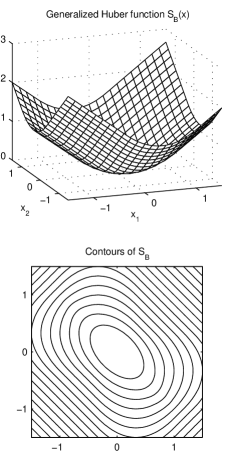
For the matrix

B=[101101],𝐵matrix101101B=\begin{bmatrix}1&0\\ 1&1\\ 0&1\end{bmatrix}, (32)

the generalized Huber function SBsubscript𝑆𝐵S_{B} is shown in Fig. 7. As shown in the contour plot, the level sets of SBsubscript𝑆𝐵S_{B} near the origin are ellipses.

Example 2.

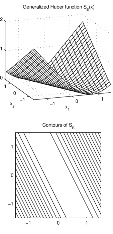
For the matrix

B=[1 0.5]𝐵delimited-[]10.5B=[1\ \ 0.5] (33)

the generalized Huber function SBsubscript𝑆𝐵S_{B} is shown in Fig. 7. The level sets of SBsubscript𝑆𝐵S_{B} are parallel lines because B𝐵B is of rank 1.

Refer to caption
Figure 6: The generalized Huber function for the matrix B𝐵B in (32).
Refer to caption
Figure 7: The generalized Huber function for the matrix B𝐵B in (33).

There is not a simple explicit formula for the generalized Huber function. But, using (31) we can derive several properties regarding the function.

Proposition 8.

Let BM×N𝐵superscript𝑀𝑁B\in\mathbb{R}^{M\times N}. The generalized Huber function satisfies

0SB(x)x1,xN.formulae-sequence0subscript𝑆𝐵𝑥subscriptdelimited-∥∥𝑥1for-all𝑥superscript𝑁0\leqslant S_{B}(x)\leqslant\lVert x\rVert_{1},\quad\forall x\in\mathbb{R}^{N}. (34)
Proof.

Using (31), we have

SB(x)subscript𝑆𝐵𝑥\displaystyle S_{B}(x) =minvN{v1+12B(xv)22}absentsubscript𝑣superscript𝑁subscriptdelimited-∥∥𝑣112superscriptsubscriptdelimited-∥∥𝐵𝑥𝑣22\displaystyle=\min_{v\in\mathbb{R}^{N}}\bigl{\{}\lVert v\rVert_{1}+\tfrac{1}{2}\lVert B(x-v)\rVert_{2}^{2}\bigr{\}}
[v1+12B(xv)22]v=xabsentsubscriptdelimited-[]subscriptdelimited-∥∥𝑣112superscriptsubscriptdelimited-∥∥𝐵𝑥𝑣22𝑣𝑥\displaystyle\leqslant\Bigl{[}\lVert v\rVert_{1}+\tfrac{1}{2}\lVert B(x-v)\rVert_{2}^{2}\Bigr{]}_{v=x}
=x1.absentsubscriptdelimited-∥∥𝑥1\displaystyle=\lVert x\rVert_{1}.

Since SBsubscript𝑆𝐵S_{B} is the minimum of a non-negative function, it also follows that SB(x)0subscript𝑆𝐵𝑥0S_{B}(x)\geqslant 0 for all x𝑥x. ∎

The following proposition accounts for the ellipses near the origin in the contour plot of the generalized Huber function in Fig. 7. (Further from the origin, the contours are not ellipsoidal.)

Proposition 9.

Let BM×N𝐵superscript𝑀𝑁B\in\mathbb{R}^{M\times N}. The generalized Huber function satisfies

SB(x)=12Bx22for allB𝖳Bx1.formulae-sequencesubscript𝑆𝐵𝑥12superscriptsubscriptdelimited-∥∥𝐵𝑥22for allsubscriptdelimited-∥∥superscript𝐵𝖳𝐵𝑥1S_{B}(x)=\tfrac{1}{2}\lVert Bx\rVert_{2}^{2}\ \ \text{for all}\ \ \lVert B^{\mathsf{T}}\!Bx\rVert_{\infty}\leqslant 1. (35)
Proof.

From (31), we have that SB(x)subscript𝑆𝐵𝑥S_{B}(x) is the minimum value of g𝑔g where g:N:𝑔superscript𝑁g\colon\mathbb{R}^{N}\to\mathbb{R} is given by

g(v)=v1+12B(xv)22.𝑔𝑣subscriptdelimited-∥∥𝑣112superscriptsubscriptdelimited-∥∥𝐵𝑥𝑣22g(v)=\lVert v\rVert_{1}+\tfrac{1}{2}\lVert B(x-v)\rVert_{2}^{2}.

Note that

g(0)=12Bx22.𝑔012superscriptsubscriptdelimited-∥∥𝐵𝑥22g(0)=\tfrac{1}{2}\lVert Bx\rVert_{2}^{2}.

Hence, it suffices to show that 00 minimizes g𝑔g if and only if B𝖳Bx1subscriptdelimited-∥∥superscript𝐵𝖳𝐵𝑥1\lVert B^{\mathsf{T}}\!Bx\rVert_{\infty}\leqslant 1. Since g𝑔g is convex, 00 minimizes g𝑔g if and only if 0g(0)0𝑔00\in\partial g(0) where g𝑔\partial g is the subdifferential of g𝑔g given by

g(v)=sign(v)+B𝖳B(vx)𝑔𝑣sign𝑣superscript𝐵𝖳𝐵𝑣𝑥\partial g(v)=\operatorname{sign}(v)+B^{\mathsf{T}}\!B(v-x)

where signsign\operatorname{sign} is the set-valued signum function,

sign(t):={{1},t>0[1, 1],t=0{1},t<0.assignsign𝑡cases1𝑡011𝑡01𝑡0\operatorname{sign}(t):=\begin{cases}\{1\},&t>0\\ [-1,\ 1],\ &t=0\\ \{-1\},&t<0.\end{cases}

It follows that 00 minimizes g𝑔g if and only if

0sign(0)B𝖳Bx0sign0superscript𝐵𝖳𝐵𝑥\displaystyle 0\in\operatorname{sign}(0)-B^{\mathsf{T}}\!Bx\quad\Leftrightarrow B𝖳Bxsuperscript𝐵𝖳𝐵𝑥\displaystyle B^{\mathsf{T}}\!Bx [1, 1]Nabsentsuperscript11𝑁\displaystyle\in[-1,\ 1]^{N}
\displaystyle\Leftrightarrow [B𝖳Bx]nsubscriptdelimited-[]superscript𝐵𝖳𝐵𝑥𝑛\displaystyle\bigl{[}B^{\mathsf{T}}\!Bx\bigr{]}_{n} [1, 1]for n=1,,Nabsent11for n=1,,N\displaystyle\in[-1,\ 1]\ \ \text{for $n=1,\dots,N$}
\displaystyle\Leftrightarrow B𝖳Bxsubscriptdelimited-∥∥superscript𝐵𝖳𝐵𝑥\displaystyle\lVert B^{\mathsf{T}}\!Bx\rVert_{\infty} 1.absent1\displaystyle\leqslant 1.

Hence, the function SBsubscript𝑆𝐵S_{B} coincides with 12B22\tfrac{1}{2}\lVert B{\,\cdot\,}\rVert_{2}^{2} on a subset of its domain. ∎

Proposition 10.

Let BM×N𝐵superscript𝑀𝑁B\in\mathbb{R}^{M\times N} and set α=B2𝛼subscriptdelimited-∥∥𝐵2\alpha=\lVert B\rVert_{2}. The generalized Huber function satisfies

SB(x)subscript𝑆𝐵𝑥\displaystyle S_{B}(x) SαI(x),xNformulae-sequenceabsentsubscript𝑆𝛼𝐼𝑥for-all𝑥superscript𝑁\displaystyle\leqslant S_{\alpha I}(x),\quad\forall x\in\mathbb{R}^{N} (36)
=nsα(xn).absentsubscript𝑛subscript𝑠𝛼subscript𝑥𝑛\displaystyle=\sum_{n}s_{\alpha}(x_{n}). (37)
Proof.

Using (31), we have

SB(x)subscript𝑆𝐵𝑥\displaystyle S_{B}(x) =minvN{v1+12B(xv)22}absentsubscript𝑣superscript𝑁subscriptdelimited-∥∥𝑣112superscriptsubscriptdelimited-∥∥𝐵𝑥𝑣22\displaystyle=\min_{v\in\mathbb{R}^{N}}\bigl{\{}\lVert v\rVert_{1}+\tfrac{1}{2}\lVert B(x-v)\rVert_{2}^{2}\bigr{\}}
minvN{v1+12B22(xv)22}absentsubscript𝑣superscript𝑁subscriptdelimited-∥∥𝑣112superscriptsubscriptdelimited-∥∥𝐵22superscriptsubscriptdelimited-∥∥𝑥𝑣22\displaystyle\leqslant\min_{v\in\mathbb{R}^{N}}\bigl{\{}\lVert v\rVert_{1}+\tfrac{1}{2}\lVert B\rVert_{2}^{2}\,\lVert(x-v)\rVert_{2}^{2}\bigr{\}}
=minvN{v1+12α2(xv)22}absentsubscript𝑣superscript𝑁subscriptdelimited-∥∥𝑣112superscript𝛼2superscriptsubscriptdelimited-∥∥𝑥𝑣22\displaystyle=\min_{v\in\mathbb{R}^{N}}\bigl{\{}\lVert v\rVert_{1}+\tfrac{1}{2}\alpha^{2}\lVert(x-v)\rVert_{2}^{2}\bigr{\}}
=minvN{v1+12α(xv)22}absentsubscript𝑣superscript𝑁subscriptdelimited-∥∥𝑣112superscriptsubscriptdelimited-∥∥𝛼𝑥𝑣22\displaystyle=\min_{v\in\mathbb{R}^{N}}\bigl{\{}\lVert v\rVert_{1}+\tfrac{1}{2}\lVert\alpha\,(x-v)\rVert_{2}^{2}\bigr{\}}
=SαI(x).absentsubscript𝑆𝛼𝐼𝑥\displaystyle=S_{\alpha I}(x).

From Proposition 7 we have (37). ∎

The Moreau envelope is well studied in convex analysis [4]. Hence, it is useful to express the generalized Huber function SBsubscript𝑆𝐵S_{B} in terms of a Moreau envelope, so we can draw on results in convex analysis to derive further properties of the generalized Huber function.

Lemma 1.

If BN×N𝐵superscript𝑁𝑁B\in\mathbb{R}^{N\times N} is invertible, then the generalized Huber function SBsubscript𝑆𝐵S_{B} can be expressed in terms of a Moreau envelope as

SB=(1B1)𝖬B.subscript𝑆𝐵superscriptsubscriptdelimited-∥∥1superscript𝐵1𝖬𝐵S_{B}=\big{(}\lVert{\,\cdot\,}\rVert_{1}\mathbin{\circ}B^{-1})^{\mathsf{M}}\mathbin{\circ}B. (38)
Proof.

Using (29), we have

SBsubscript𝑆𝐵\displaystyle S_{B} =1(1222B)\displaystyle=\lVert{\,\cdot\,}\rVert_{1}\mbox{\footnotesize$\;\square\;$}\bigr{(}\tfrac{1}{2}\lVert{\,\cdot\,}\rVert_{2}^{2}\mathbin{\circ}B\bigr{)}
=(1(1222B))B1B\displaystyle=\Bigl{(}\lVert{\,\cdot\,}\rVert_{1}\mbox{\footnotesize$\;\square\;$}\bigr{(}\tfrac{1}{2}\lVert{\,\cdot\,}\rVert_{2}^{2}\mathbin{\circ}B\bigr{)}\Bigr{)}\mathbin{\circ}B^{-1}\mathbin{\circ}B
=((1B1)(1222))Babsentsubscriptdelimited-∥∥1superscript𝐵112superscriptsubscriptdelimited-∥∥22𝐵\displaystyle=\Bigl{(}\bigl{(}\lVert{\,\cdot\,}\rVert_{1}\mathbin{\circ}B^{-1}\bigr{)}\mbox{\footnotesize$\;\square\;$}\bigl{(}\tfrac{1}{2}\lVert{\,\cdot\,}\rVert_{2}^{2}\bigr{)}\Bigr{)}\mathbin{\circ}B
=(1B1)𝖬B.absentsuperscriptsubscriptdelimited-∥∥1superscript𝐵1𝖬𝐵\displaystyle=\bigl{(}\lVert{\,\cdot\,}\rVert_{1}\mathbin{\circ}B^{-1}\bigr{)}^{\mathsf{M}}\mathbin{\circ}B.\qed
Lemma 2.

If BM×N𝐵superscript𝑀𝑁B\in\mathbb{R}^{M\times N} has full row-rank, then the generalized Huber function SBsubscript𝑆𝐵S_{B} can be expressed in terms of a Moreau envelope as

SB=(dB+)𝖬Bsubscript𝑆𝐵superscript𝑑superscript𝐵𝖬𝐵S_{B}=\big{(}d\mathbin{\circ}B^{\mathsf{+}})^{\mathsf{M}}\mathbin{\circ}B (39)

where d:N:𝑑superscript𝑁d\colon\mathbb{R}^{N}\to\mathbb{R} is the convex distance function

d(x)=minwnullBxw1d(x)=\min_{w\in\operatorname{null}B}\lVert x-w\rVert_{1} (40)

which represents the distance from the point xN𝑥superscript𝑁x\in\mathbb{R}^{N} to the null space of B𝐵B as measured by the 1subscript1\ell_{1} norm.

Proof.

Using (31), we have

SB(x)subscript𝑆𝐵𝑥\displaystyle S_{B}(x) =minvN{v1+12B(xv)22}absentsubscript𝑣superscript𝑁subscriptdelimited-∥∥𝑣112superscriptsubscriptdelimited-∥∥𝐵𝑥𝑣22\displaystyle=\min_{v\in\mathbb{R}^{N}}\bigl{\{}\lVert v\rVert_{1}+\tfrac{1}{2}\lVert B(x-v)\rVert_{2}^{2}\bigr{\}}
=f(Bx)absent𝑓𝐵𝑥\displaystyle=f(Bx)

where f:M:𝑓superscript𝑀f\colon\mathbb{R}^{M}\to\mathbb{R} is given by

f(z)𝑓𝑧\displaystyle f(z) =minvN{v1+12zBv22}absentsubscript𝑣superscript𝑁subscriptdelimited-∥∥𝑣112superscriptsubscriptdelimited-∥∥𝑧𝐵𝑣22\displaystyle=\min_{v\in\mathbb{R}^{N}}\bigl{\{}\lVert v\rVert_{1}+\tfrac{1}{2}\lVert z-Bv\rVert_{2}^{2}\,\bigr{\}}
=minu(nullB)minwnullB{u+w1+12zB(u+w)22}absentsubscript𝑢superscriptnull𝐵perpendicular-tosubscript𝑤null𝐵subscriptdelimited-∥∥𝑢𝑤112superscriptsubscriptdelimited-∥∥𝑧𝐵𝑢𝑤22\displaystyle=\min_{u\in(\operatorname{null}B)^{\perp}}\;\min_{w\in\operatorname{null}B}\bigl{\{}\lVert u+w\rVert_{1}+\tfrac{1}{2}\lVert z-B(u+w)\rVert_{2}^{2}\,\bigr{\}}
=minu(nullB)minwnullB{u+w1+12zBu22}absentsubscript𝑢superscriptnull𝐵perpendicular-tosubscript𝑤null𝐵subscriptdelimited-∥∥𝑢𝑤112superscriptsubscriptdelimited-∥∥𝑧𝐵𝑢22\displaystyle=\min_{u\in(\operatorname{null}B)^{\perp}}\;\min_{w\in\operatorname{null}B}\bigl{\{}\lVert u+w\rVert_{1}+\tfrac{1}{2}\lVert z-Bu\rVert_{2}^{2}\,\bigr{\}}
=minu(nullB){d(u)+12zBu22}absentsubscript𝑢superscriptnull𝐵perpendicular-to𝑑𝑢12superscriptsubscriptdelimited-∥∥𝑧𝐵𝑢22\displaystyle=\min_{u\in(\operatorname{null}B)^{\perp}}\bigl{\{}d(u)+\tfrac{1}{2}\lVert z-Bu\rVert_{2}^{2}\,\bigr{\}}

where d𝑑d is the convex function given by (40). The fact that d𝑑d is convex follows from Proposition 8.26 of [4] and Examples 3.16 and 3.17 of [8]. Since (nullB)=rangeB𝖳superscriptnull𝐵perpendicular-torangesuperscript𝐵𝖳(\operatorname{null}B)^{\perp}=\operatorname{range}B^{\mathsf{T}},

f(z)𝑓𝑧\displaystyle f(z) =minurangeB𝖳{d(u)+12zBu22}absentsubscript𝑢rangesuperscript𝐵𝖳𝑑𝑢12superscriptsubscriptdelimited-∥∥𝑧𝐵𝑢22\displaystyle=\min_{u\in\operatorname{range}B^{\mathsf{T}}}\bigl{\{}d(u)+\tfrac{1}{2}\lVert z-Bu\rVert_{2}^{2}\bigr{\}}
=minvM{d(B𝖳v)+12zBB𝖳v22}absentsubscript𝑣superscript𝑀𝑑superscript𝐵𝖳𝑣12superscriptsubscriptdelimited-∥∥𝑧𝐵superscript𝐵𝖳𝑣22\displaystyle=\min_{v\in\mathbb{R}^{M}}\bigl{\{}d(B^{\mathsf{T}}\!v)+\tfrac{1}{2}\lVert z-BB^{\mathsf{T}}\!v\rVert_{2}^{2}\bigr{\}}
=minvM{d(B𝖳(BB𝖳)1v)+12zBB𝖳(BB𝖳)1v22}absentsubscript𝑣superscript𝑀𝑑superscript𝐵𝖳superscript𝐵superscript𝐵𝖳1𝑣12superscriptsubscriptdelimited-∥∥𝑧𝐵superscript𝐵𝖳superscript𝐵superscript𝐵𝖳1𝑣22\displaystyle=\min_{v\in\mathbb{R}^{M}}\bigl{\{}d(B^{\mathsf{T}}(BB^{\mathsf{T}})^{-1}v)+\tfrac{1}{2}\lVert z-BB^{\mathsf{T}}(BB^{\mathsf{T}})^{-1}v\rVert_{2}^{2}\bigr{\}}
=minvM{d(B+v)+12zv22}absentsubscript𝑣superscript𝑀𝑑superscript𝐵𝑣12superscriptsubscriptdelimited-∥∥𝑧𝑣22\displaystyle=\min_{v\in\mathbb{R}^{M}}\bigl{\{}d(B^{\mathsf{+}}v)+\tfrac{1}{2}\lVert z-v\rVert_{2}^{2}\bigr{\}}
=(d(B+))𝖬(z).\displaystyle=\bigl{(}d(B^{\mathsf{+}}{\,\cdot\,})\bigr{)}^{\mathsf{M}}(z).

Hence, SB(x)=(d(B+))𝖬(Bx)S_{B}(x)=\bigl{(}d(B^{\mathsf{+}}{\,\cdot\,})\bigr{)}^{\mathsf{M}}(Bx) which completes the proof. ∎

Note that (39) reduces to (38) when B𝐵B is invertible. (Suppose B𝐵B is invertible. Then nullB={0}null𝐵0\operatorname{null}B=\{0\}; hence d(x)=x1𝑑𝑥subscriptdelimited-∥∥𝑥1d(x)=\lVert x\rVert_{1} in (40). Additionally, B+=B1superscript𝐵superscript𝐵1B^{\mathsf{+}}=B^{-1}.)

Proposition 11.

The generalized Huber function is differentiable.

Proof.

By Lemma 2, SBsubscript𝑆𝐵S_{B} is the composition of a Moreau envelope of a convex function and a linear function. Additionally, by Proposition 5, SBΓ0(N)subscript𝑆𝐵subscriptΓ0superscript𝑁S_{B}\in\Gamma_{0}(\mathbb{R}^{N}). By Proposition 12.29 in [4], it follows that SBsubscript𝑆𝐵S_{B} is differentiable. ∎

The following result regards the gradient of the generalized Huber function. This result will be used in Sec. 5 to show the generalized MC penalty defined therein constitutes a valid penalty.

Lemma 3.

The gradient of the generalized Huber function SB:N:subscript𝑆𝐵superscript𝑁S_{B}\colon\mathbb{R}^{N}\to\mathbb{R} satisfies

SB(x)1for allxN.formulae-sequencesubscriptdelimited-∥∥subscript𝑆𝐵𝑥1for all𝑥superscript𝑁\lVert\nabla S_{B}(x)\rVert_{\infty}\leqslant 1\ \ \text{for all}\ x\in\mathbb{R}^{N}. (41)
Proof.

Since SBsubscript𝑆𝐵S_{B} is convex and differentiable, we have

SB(v)+[SB(v)]𝖳(xv)SB(x),xN,vN.formulae-sequencesubscript𝑆𝐵𝑣superscriptdelimited-[]subscript𝑆𝐵𝑣𝖳𝑥𝑣subscript𝑆𝐵𝑥formulae-sequencefor-all𝑥superscript𝑁for-all𝑣superscript𝑁S_{B}(v)+\bigl{[}\nabla S_{B}(v)\bigr{]}^{\mathsf{T}}(x-v)\leqslant S_{B}(x),\quad\forall x\in\mathbb{R}^{N},\;\forall v\in\mathbb{R}^{N}.

Using Proposition 8, it follows that

SB(v)+[SB(v)]𝖳(xv)x1,xN,vN.formulae-sequencesubscript𝑆𝐵𝑣superscriptdelimited-[]subscript𝑆𝐵𝑣𝖳𝑥𝑣subscriptdelimited-∥∥𝑥1formulae-sequencefor-all𝑥superscript𝑁for-all𝑣superscript𝑁S_{B}(v)+\bigl{[}\nabla S_{B}(v)\bigr{]}^{\mathsf{T}}(x-v)\leqslant\lVert x\rVert_{1},\quad\forall x\in\mathbb{R}^{N},\;\forall v\in\mathbb{R}^{N}.

Let x=(0,,0,t,0,,0)𝑥00𝑡00x=(0,\ldots,0,t,0,\ldots,0) where t𝑡t is in position n𝑛n. It follows that

c(v)+[SB(v)]nt|t|,t,vNformulae-sequence𝑐𝑣subscriptdelimited-[]subscript𝑆𝐵𝑣𝑛𝑡𝑡formulae-sequencefor-all𝑡for-all𝑣superscript𝑁c(v)+\bigl{[}\nabla S_{B}(v)\bigr{]}_{n}\,t\leqslant\lvert t\rvert,\quad\forall t\in\mathbb{R},\;\forall v\in\mathbb{R}^{N} (42)

where c(v)𝑐𝑣c(v)\in\mathbb{R} does not depend on t𝑡t. It follows from (42) that |[SB(v)]n|1subscriptdelimited-[]subscript𝑆𝐵𝑣𝑛1\lvert[\nabla S_{B}(v)]_{n}\rvert\leqslant 1. ∎

The generalized Huber function can be evaluated by taking the pointwise minimum of numerous simpler functions (comprising quadratics, absolute values, and linear functions). This generalizes the situation for the scalar Huber function, which can be evaluated as the pointwise minimum of three functions, as expressed in (11) and illustrated in Fig. 2. Unfortunately, evaluating the generalized Huber function on Nsuperscript𝑁\mathbb{R}^{N} this way requires the evaluation of 3Nsuperscript3𝑁3^{N} simpler functions, which is not practical except for small N𝑁N. In turn, the evaluation of the GMC penalty is also impractical. However, we do not need to explicitly evaluate these functions to utilize them for sparse regularization, as shown in Sec. 7. For this paper, we compute these functions on 2superscript2\mathbb{R}^{2} only for the purpose of illustration (Figs. 7 and 7).

5 Generalized MC Penalty

In this section, we propose a multivariate generalization of the MC penalty (12). The basic idea is to generalize (22) using the 1subscript1\ell_{1} norm and the generalized Huber function.

Definition 7.

Let BM×N𝐵superscript𝑀𝑁B\in\mathbb{R}^{M\times N}. We define the generalized MC (GMC) penalty function ψB:N:subscript𝜓𝐵superscript𝑁\psi_{B}\colon\mathbb{R}^{N}\to\mathbb{R} as

ψB(x):=x1SB(x)assignsubscript𝜓𝐵𝑥subscriptdelimited-∥∥𝑥1subscript𝑆𝐵𝑥\psi_{B}(x):=\lVert x\rVert_{1}-S_{B}(x) (43)

where SBsubscript𝑆𝐵S_{B} is the generalized Huber function (29).

The GMC penalty reduces to a separable penalty when B𝖳Bsuperscript𝐵𝖳𝐵B^{\mathsf{T}}\!B is diagonal.

Proposition 12.

Let BM×N𝐵superscript𝑀𝑁B\in\mathbb{R}^{M\times N}. If B𝖳Bsuperscript𝐵𝖳𝐵B^{\mathsf{T}}\!B is a diagonal matrix, then ψBsubscript𝜓𝐵\psi_{B} is separable (additive), comprising a sum of scalar MC penalties. Specifically,

B𝖳B=diag(α12,,αN2)ψB(x)=nϕαn(xn)formulae-sequencesuperscript𝐵𝖳𝐵diagsuperscriptsubscript𝛼12superscriptsubscript𝛼𝑁2subscript𝜓𝐵𝑥subscript𝑛subscriptitalic-ϕsubscript𝛼𝑛subscript𝑥𝑛B^{\mathsf{T}}\!B=\mathrm{diag}(\alpha_{1}^{2},\dots,\alpha_{N}^{2})\ \ \implies\ \ \psi_{B}(x)=\sum_{n}\phi_{\alpha_{n}}(x_{n})

where ϕbsubscriptitalic-ϕ𝑏\phi_{b} is the scaled MC penalty (22). If B𝖳B=0superscript𝐵𝖳𝐵0B^{\mathsf{T}}\!B=0, then ψB(x)=x1subscript𝜓𝐵𝑥subscriptdelimited-∥∥𝑥1\psi_{B}(x)=\lVert x\rVert_{1}.

Proof.

If B𝖳B=diag(α12,,αN2)superscript𝐵𝖳𝐵diagsuperscriptsubscript𝛼12superscriptsubscript𝛼𝑁2B^{\mathsf{T}}\!B=\mathrm{diag}(\alpha_{1}^{2},\dots,\alpha_{N}^{2}), then by Proposition 7 we have

ψB(x)subscript𝜓𝐵𝑥\displaystyle\psi_{B}(x) =x1nsαn(xn)absentsubscriptdelimited-∥∥𝑥1subscript𝑛subscript𝑠subscript𝛼𝑛subscript𝑥𝑛\displaystyle=\lVert x\rVert_{1}-\sum_{n}s_{\alpha_{n}}(x_{n})
=n|xn|sαn(xn)absentsubscript𝑛subscript𝑥𝑛subscript𝑠subscript𝛼𝑛subscript𝑥𝑛\displaystyle=\sum_{n}\,\lvert x_{n}\rvert-s_{\alpha_{n}}(x_{n})

which proves the result in light of definition (22). ∎

Refer to caption
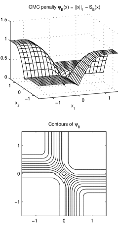
Figure 8: The GMC penalty for the matrix B𝐵B in (32).
Refer to caption
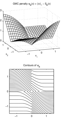
Figure 9: The GMC penalty for the matrix B𝐵B in (33).

The most interesting case (the case that motivates the GMC penalty) is the case where B𝖳Bsuperscript𝐵𝖳𝐵B^{\mathsf{T}}\!B is a non-diagonal matrix. If B𝖳Bsuperscript𝐵𝖳𝐵B^{\mathsf{T}}\!B is non-diagonal, then the GMC penalty is non-separable.

Example 3.

For the matrices B𝐵B given in (32) and (33), the GMC penalty is illustrated in Fig. 9 and Fig. 9, respectively.

The following corollaries follow directly from Propositions 8 and 9.

Corollary 1.

The generalized MC penalty satisfies

0ψB(x)x1for all xN.formulae-sequence0subscript𝜓𝐵𝑥subscriptdelimited-∥∥𝑥1for all xN.0\leqslant\psi_{B}(x)\leqslant\lVert x\rVert_{1}\quad\text{for all $x\in\mathbb{R}^{N}$.} (44)
Corollary 2.

Given BM×N𝐵superscript𝑀𝑁B\in\mathbb{R}^{M\times N}, the generalized MC penalty satisfies

ψB(x)=x112Bx22for allB𝖳Bx1.formulae-sequencesubscript𝜓𝐵𝑥subscriptdelimited-∥∥𝑥112superscriptsubscriptdelimited-∥∥𝐵𝑥22for allsubscriptdelimited-∥∥superscript𝐵𝖳𝐵𝑥1\psi_{B}(x)=\lVert x\rVert_{1}-\tfrac{1}{2}\lVert Bx\rVert_{2}^{2}\ \ \text{for all}\ \ \lVert B^{\mathsf{T}}\!Bx\rVert_{\infty}\leqslant 1. (45)

The corollaries imply that around zero the generalized MC penalty approximates the 1subscript1\ell_{1} norm (from below), i.e., ψB(x)x1subscript𝜓𝐵𝑥subscriptdelimited-∥∥𝑥1\psi_{B}(x)\approx\lVert x\rVert_{1} for x0𝑥0x\approx 0.

The generalized MC penalty has a basic property expected of a regularization function; namely, that large values are penalized more than (or the same as) small values. Specifically, if v,xN𝑣𝑥superscript𝑁v,x\in\mathbb{R}^{N} with |vi||xi|subscript𝑣𝑖subscript𝑥𝑖\lvert v_{i}\rvert\geqslant\lvert x_{i}\rvert and signvi=signxisignsubscript𝑣𝑖signsubscript𝑥𝑖\operatorname{sign}{v_{i}}=\operatorname{sign}{x_{i}} for i=1,,N𝑖1𝑁i=1,\ldots,N, then ψB(v)ψB(x)subscript𝜓𝐵𝑣subscript𝜓𝐵𝑥\psi_{B}(v)\geqslant\psi_{B}(x). That is, in any given quadrant, the function ψB(x)subscript𝜓𝐵𝑥\psi_{B}(x) is a non-decreasing function in each |xi|subscript𝑥𝑖\lvert x_{i}\rvert. This is formalized in the following proposition, and illustrated in Figs. 9 and 9. Basically, the gradient of ψBsubscript𝜓𝐵\psi_{B} points away from the origin.

Proposition 13.

Let xN𝑥superscript𝑁x\in\mathbb{R}^{N} with xi0subscript𝑥𝑖0x_{i}\neq 0. The generalized MC penalty ψBsubscript𝜓𝐵\psi_{B} has the property that [ψB(x)]isubscriptdelimited-[]subscript𝜓𝐵𝑥𝑖[\nabla\psi_{B}(x)]_{i} either has the same sign as xisubscript𝑥𝑖x_{i} or is equal to zero.

Proof.

Let xN𝑥superscript𝑁x\in\mathbb{R}^{N} with xi0subscript𝑥𝑖0x_{i}\neq 0. Then, from the definition of the MC penalty,

ψBxi(x)=sign(xi)SBxi(x).subscript𝜓𝐵subscript𝑥𝑖𝑥signsubscript𝑥𝑖subscript𝑆𝐵subscript𝑥𝑖𝑥\frac{\partial\psi_{B}}{\partial{x_{i}}}(x)=\operatorname{sign}(x_{i})-\frac{\partial S_{B}}{\partial{x_{i}}}(x).

From Lemma 3, |SB(x)/xi|1subscript𝑆𝐵𝑥subscript𝑥𝑖1\lvert\partial S_{B}(x)/\partial x_{i}\rvert\leqslant 1. Hence ψB(x)/xi0subscript𝜓𝐵𝑥subscript𝑥𝑖0\partial\psi_{B}(x)/\partial x_{i}\geqslant 0 when xi>0subscript𝑥𝑖0x_{i}>0, and ψB(x)/xi0subscript𝜓𝐵𝑥subscript𝑥𝑖0\partial\psi_{B}(x)/\partial x_{i}\leqslant 0 when xi<0subscript𝑥𝑖0x_{i}<0. ∎

A penalty function not satisfying Proposition 13 would not be considered an effective sparsity-inducing regularizer.

6 Sparse Regularization

In this section, we consider how to set the GMC penalty to maintain the convexity of the regularized least square cost function. To that end, the condition (47) below generalizes the scalar convexity condition (25).

Theorem 1.

Let yM𝑦superscript𝑀y\in\mathbb{R}^{M}, AM×N𝐴superscript𝑀𝑁A\in\mathbb{R}^{M\times N}, and λ>0𝜆0{\lambda}>0. Define F:N:𝐹superscript𝑁F\colon\mathbb{R}^{N}\to\mathbb{R} as

F(x)=12yAx22+λψB(x)𝐹𝑥12superscriptsubscriptdelimited-∥∥𝑦𝐴𝑥22𝜆subscript𝜓𝐵𝑥F(x)=\frac{1}{2}\lVert y-Ax\rVert_{2}^{2}+{\lambda}\,\psi_{B}(x) (46)

where ψB:N:subscript𝜓𝐵superscript𝑁\psi_{B}\colon\mathbb{R}^{N}\to\mathbb{R} is the generalized MC penalty (43). If

B𝖳B1λA𝖳Aprecedes-or-equalssuperscript𝐵𝖳𝐵1𝜆superscript𝐴𝖳𝐴B^{\mathsf{T}}\!B\preccurlyeq\frac{1}{{\lambda}}A^{\mathsf{T}}\!A (47)

then F𝐹F is a convex function.

Proof.

Write F𝐹F as

F(x)𝐹𝑥\displaystyle F(x) =12yAx22+λ(x1SB(x))absent12superscriptsubscriptdelimited-∥∥𝑦𝐴𝑥22𝜆subscriptdelimited-∥∥𝑥1subscript𝑆𝐵𝑥\displaystyle=\tfrac{1}{2}\lVert y-Ax\rVert_{2}^{2}+{\lambda}\,\bigl{(}\lVert x\rVert_{1}-S_{B}(x)\bigr{)}
=12yAx22+λx1minvN{λv1+λ2B(xv)22}absent12superscriptsubscriptdelimited-∥∥𝑦𝐴𝑥22𝜆subscriptdelimited-∥∥𝑥1subscript𝑣superscript𝑁𝜆subscriptdelimited-∥∥𝑣1𝜆2superscriptsubscriptdelimited-∥∥𝐵𝑥𝑣22\displaystyle=\tfrac{1}{2}\lVert y-Ax\rVert_{2}^{2}+{\lambda}\,\lVert x\rVert_{1}-\min_{v\in\mathbb{R}^{N}}\big{\{}{\lambda}\lVert v\rVert_{1}+\tfrac{{\lambda}}{2}\lVert B(x-v)\rVert_{2}^{2}\big{\}}
=maxvN{12yAx22+λx1λv1λ2B(xv)22}absentsubscript𝑣superscript𝑁12superscriptsubscriptdelimited-∥∥𝑦𝐴𝑥22𝜆subscriptdelimited-∥∥𝑥1𝜆subscriptdelimited-∥∥𝑣1𝜆2superscriptsubscriptdelimited-∥∥𝐵𝑥𝑣22\displaystyle=\max_{v\in\mathbb{R}^{N}}\big{\{}\tfrac{1}{2}\lVert y-Ax\rVert_{2}^{2}+{\lambda}\,\lVert x\rVert_{1}-{\lambda}\lVert v\rVert_{1}-\tfrac{{\lambda}}{2}\lVert B(x-v)\rVert_{2}^{2}\big{\}}
=maxvN{12x𝖳(A𝖳AλB𝖳B)x+λx1+g(x,v)}absentsubscript𝑣superscript𝑁12superscript𝑥𝖳superscript𝐴𝖳𝐴𝜆superscript𝐵𝖳𝐵𝑥𝜆subscriptdelimited-∥∥𝑥1𝑔𝑥𝑣\displaystyle=\max_{v\in\mathbb{R}^{N}}\big{\{}\tfrac{1}{2}x^{\mathsf{T}}\!\bigl{(}A^{\mathsf{T}}\!A-{\lambda}B^{\mathsf{T}}\!B\bigr{)}x+{\lambda}\lVert x\rVert_{1}+g(x,v)\big{\}}
=12x𝖳(A𝖳AλB𝖳B)x+λx1+maxvNg(x,v)absent12superscript𝑥𝖳superscript𝐴𝖳𝐴𝜆superscript𝐵𝖳𝐵𝑥𝜆subscriptdelimited-∥∥𝑥1subscript𝑣superscript𝑁𝑔𝑥𝑣\displaystyle=\tfrac{1}{2}x^{\mathsf{T}}\!\bigl{(}A^{\mathsf{T}}\!A-{\lambda}B^{\mathsf{T}}\!B\bigr{)}x+{\lambda}\lVert x\rVert_{1}+\max_{v\in\mathbb{R}^{N}}g(x,v)

where g𝑔g is affine in x𝑥x. The last term is convex as it is the pointwise maximum of a set of convex functions (Proposition 8.14 in [4]). Hence, F𝐹F is convex if A𝖳AλB𝖳Bsuperscript𝐴𝖳𝐴𝜆superscript𝐵𝖳𝐵A^{\mathsf{T}}\!A-{\lambda}B^{\mathsf{T}}\!B is positive semidefinite. ∎

The convexity condition (47) is easily satisfied. Given A𝐴A, we may simply set

B=γ/λA,0γ1.formulae-sequence𝐵𝛾𝜆𝐴0𝛾1B=\sqrt{\gamma/{\lambda}\,}A,\quad 0\leqslant\gamma\leqslant 1. (48)

Then B𝖳B=(γ/λ)A𝖳Asuperscript𝐵𝖳𝐵𝛾𝜆superscript𝐴𝖳𝐴B^{\mathsf{T}}\!B=(\gamma/{\lambda})A^{\mathsf{T}}\!A which satisfies (47) when γ1𝛾1\gamma\leqslant 1. The parameter γ𝛾\gamma controls the non-convexity of the penalty ψBsubscript𝜓𝐵\psi_{B}. If γ=0𝛾0\gamma=0, then B=0𝐵0B=0 and the penalty reduces to the 1subscript1\ell_{1} norm. If γ=1𝛾1\gamma=1, then (47) is satisfied with equality and the penalty is ‘maximally’ non-convex. In practice, we use a nominal range of 0.5γ0.80.5𝛾0.80.5\leqslant\gamma\leqslant 0.8.


When A𝖳Asuperscript𝐴𝖳𝐴A^{\mathsf{T}}\!A is diagonal, the proposed methodology reduces to element-wise firm thresholding.

Proposition 14.

Let yM𝑦superscript𝑀y\in\mathbb{R}^{M}, AM×N𝐴superscript𝑀𝑁A\in\mathbb{R}^{M\times N}, and λ>0𝜆0{\lambda}>0. If A𝖳Asuperscript𝐴𝖳𝐴A^{\mathsf{T}}\!A is diagonal with positive diagonal entries and B𝐵B is given by (48), then the minimizer of the cost function F𝐹F in (46) is given by element-wise firm thresholding. Specifically, if

A𝖳A=diag(α12,,αN2),superscript𝐴𝖳𝐴diagsuperscriptsubscript𝛼12superscriptsubscript𝛼𝑁2A^{\mathsf{T}}\!A=\mathrm{diag}(\alpha_{1}^{2},\dots,\alpha_{N}^{2}), (49)

then

xn𝗈𝗉𝗍=firm([A𝖳y]n/αn2;λ/αn2,λ/(γαn2))subscriptsuperscript𝑥𝗈𝗉𝗍𝑛firmsubscriptdelimited-[]superscript𝐴𝖳𝑦𝑛superscriptsubscript𝛼𝑛2𝜆superscriptsubscript𝛼𝑛2𝜆𝛾superscriptsubscript𝛼𝑛2x^{\mathsf{opt}}_{n}=\operatorname{firm}([A^{\mathsf{T}}\!y]_{n}/\alpha_{n}^{2};{\lambda}/\alpha_{n}^{2},{\lambda}/(\gamma\alpha_{n}^{2})) (50)

when 0<γ10𝛾10<\gamma\leqslant 1, and

xn𝗈𝗉𝗍=soft([A𝖳y]n/αn2;λ/αn2)subscriptsuperscript𝑥𝗈𝗉𝗍𝑛softsubscriptdelimited-[]superscript𝐴𝖳𝑦𝑛superscriptsubscript𝛼𝑛2𝜆superscriptsubscript𝛼𝑛2x^{\mathsf{opt}}_{n}=\operatorname{soft}([A^{\mathsf{T}}y]_{n}/\alpha_{n}^{2};{\lambda}/\alpha_{n}^{2}) (51)

when γ=0𝛾0\gamma=0.

Proof.

If A𝖳A=diag(α12,,αN2)superscript𝐴𝖳𝐴diagsuperscriptsubscript𝛼12superscriptsubscript𝛼𝑁2A^{\mathsf{T}}\!A=\mathrm{diag}(\alpha_{1}^{2},\dots,\alpha_{N}^{2}), then

12yAx2212superscriptsubscriptdelimited-∥∥𝑦𝐴𝑥22\displaystyle\tfrac{1}{2}\lVert y-Ax\rVert_{2}^{2} =12y𝖳yx𝖳A𝖳y+12x𝖳A𝖳Axabsent12superscript𝑦𝖳𝑦superscript𝑥𝖳superscript𝐴𝖳𝑦12superscript𝑥𝖳superscript𝐴𝖳𝐴𝑥\displaystyle=\tfrac{1}{2}y^{\mathsf{T}}\!y-x^{\mathsf{T}}\!A^{\mathsf{T}}y+\tfrac{1}{2}x^{\mathsf{T}}\!A^{\mathsf{T}}\!Ax
=12y𝖳y+n(xn[A𝖳y]n+12αn2xn2)\displaystyle=\tfrac{1}{2}y^{\mathsf{T}}\!y+\sum_{n}\bigr{(}-x_{n}[A^{\mathsf{T}}\!y]_{n}+\tfrac{1}{2}\alpha_{n}^{2}x_{n}^{2}\bigl{)}
=n12([A𝖳y]n/αnαnxn)2+Cabsentsubscript𝑛12superscriptsubscriptdelimited-[]superscript𝐴𝖳𝑦𝑛subscript𝛼𝑛subscript𝛼𝑛subscript𝑥𝑛2𝐶\displaystyle=\sum_{n}\tfrac{1}{2}\bigl{(}[A^{\mathsf{T}}\!y]_{n}/\alpha_{n}-\alpha_{n}x_{n}\bigr{)}^{2}+C

where C𝐶C does not depend on x𝑥x. If B𝐵B is given by (48), then

B𝖳B=(γ/λ)diag(α12,,αN2).superscript𝐵𝖳𝐵𝛾𝜆diagsuperscriptsubscript𝛼12superscriptsubscript𝛼𝑁2B^{\mathsf{T}}\!B=(\gamma/{\lambda})\,\mathrm{diag}(\alpha_{1}^{2},\dots,\alpha_{N}^{2}).

Using Proposition 12, we have

ψB(x)=nϕαnγ/λ(xn).subscript𝜓𝐵𝑥subscript𝑛subscriptitalic-ϕsubscript𝛼𝑛𝛾𝜆subscript𝑥𝑛\psi_{B}(x)=\sum_{n}\phi_{\alpha_{n}\sqrt{\gamma/{\lambda}}}(x_{n}).

Hence, F𝐹F in (46) is given by

F(x)=n[12([A𝖳y]n/αnαnxn)2+λϕαnγ/λ(xn)]+C𝐹𝑥subscript𝑛delimited-[]12superscriptsubscriptdelimited-[]superscript𝐴𝖳𝑦𝑛subscript𝛼𝑛subscript𝛼𝑛subscript𝑥𝑛2𝜆subscriptitalic-ϕsubscript𝛼𝑛𝛾𝜆subscript𝑥𝑛𝐶F(x)=\sum_{n}\left[\tfrac{1}{2}\bigl{(}[A^{\mathsf{T}}\!y]_{n}/\alpha_{n}-\alpha_{n}x_{n}\bigr{)}^{2}+{\lambda}\phi_{\alpha_{n}\sqrt{\gamma/{\lambda}}}(x_{n})\right]+C

and so (50) follows from (28). ∎

7 Optimization Algorithm

Even though the GMC penalty does not have a simple explicit formula, a global minimizer of the sparse-regularized cost function (46) can be readily calculated using proximal algorithms. It is not necessary to explicitly evaluate the GMC penalty or its gradient.

To use proximal algorithms to minimize the cost function F𝐹F in (46) when B𝐵B satisfies (47), we rewrite it as a saddle-point problem:

(x𝗈𝗉𝗍,v𝗈𝗉𝗍)=argminxNmaxvNF(x,v)superscript𝑥𝗈𝗉𝗍superscript𝑣𝗈𝗉𝗍subscript𝑥superscript𝑁subscript𝑣superscript𝑁𝐹𝑥𝑣(x^{\mathsf{opt}},\,v^{\mathsf{opt}})=\arg\min_{x\in\mathbb{R}^{N}}\max_{v\in\mathbb{R}^{N}}F(x,v) (52)

where

F(x,v)=12yAx22+λx1λv1λ2B(xv)22𝐹𝑥𝑣12superscriptsubscriptdelimited-∥∥𝑦𝐴𝑥22𝜆subscriptdelimited-∥∥𝑥1𝜆subscriptdelimited-∥∥𝑣1𝜆2superscriptsubscriptdelimited-∥∥𝐵𝑥𝑣22F(x,v)=\frac{1}{2}\lVert y-Ax\rVert_{2}^{2}+{\lambda}\,\lVert x\rVert_{1}-{\lambda}\lVert v\rVert_{1}-\frac{{\lambda}}{2}\lVert B(x-v)\rVert_{2}^{2} (53)

If we use (48) with 0γ10𝛾10\leqslant\gamma\leqslant 1, then the saddle function is given by

F(x,v)=12yAx22+λx1λv1γ2A(xv)22.𝐹𝑥𝑣12superscriptsubscriptdelimited-∥∥𝑦𝐴𝑥22𝜆subscriptdelimited-∥∥𝑥1𝜆subscriptdelimited-∥∥𝑣1𝛾2superscriptsubscriptdelimited-∥∥𝐴𝑥𝑣22F(x,v)=\frac{1}{2}\lVert y-Ax\rVert_{2}^{2}+{\lambda}\,\lVert x\rVert_{1}-{\lambda}\lVert v\rVert_{1}-\frac{\gamma}{2}\lVert A(x-v)\rVert_{2}^{2}. (54)

These saddle-point problems are instances of monotone inclusion problems. Hence, the solution can be obtained using the forward-backward (FB) algorithm for such a problems; see Theorem 25.8 of Ref. [4]. The FB algorithm involves only simple computational steps (soft-thresholding and the operators A𝐴A and A𝖳superscript𝐴𝖳A^{\mathsf{T}}).

Proposition 15.

Let λ>0𝜆0{\lambda}>0 and 0γ<10𝛾10\leqslant\gamma<1. Let yN𝑦superscript𝑁y\in\mathbb{R}^{N} and AM×N𝐴superscript𝑀𝑁A\in\mathbb{R}^{M\times N}. Then a saddle-point (x𝗈𝗉𝗍,v𝗈𝗉𝗍)superscript𝑥𝗈𝗉𝗍superscript𝑣𝗈𝗉𝗍(x^{\mathsf{opt}},\,v^{\mathsf{opt}}) of F𝐹F in (54) can be obtained by the iterative algorithm:

Set ρ=max{1,γ/(1γ)}A𝖳A2Set 𝜌1𝛾1𝛾subscriptdelimited-∥∥superscript𝐴𝖳𝐴2\displaystyle\text{Set }\rho=\max\{1,\,\gamma/(1-\gamma)\}\,\lVert A^{\mathsf{T}}\!A\rVert_{2}
Set μ:0<μ<2/ρ:Set 𝜇0𝜇2𝜌\displaystyle\text{Set }\mu:0<\mu<2/\rho
For i=0,1,2,𝑖012italic-…i=0,1,2,\dots
w(i)=x(i)μA𝖳(A(x(i)+γ(v(i)x(i)))y)superscript𝑤𝑖superscript𝑥𝑖𝜇superscript𝐴𝖳𝐴superscript𝑥𝑖𝛾superscript𝑣𝑖superscript𝑥𝑖𝑦\displaystyle\quad w^{(i)}=x^{(i)}-\mu A^{\mathsf{T}}\!\bigl{(}A(x^{(i)}+\gamma(v^{(i)}-x^{(i)}))-y\bigr{)}
u(i)=v(i)μγA𝖳A(v(i)x(i))superscript𝑢𝑖superscript𝑣𝑖𝜇𝛾superscript𝐴𝖳𝐴superscript𝑣𝑖superscript𝑥𝑖\displaystyle\quad u^{(i)}=v^{(i)}-\mu\gamma A^{\mathsf{T}}\!A(v^{(i)}-x^{(i)})
x(i+1)=soft(w(i),μλ)superscript𝑥𝑖1softsuperscript𝑤𝑖𝜇𝜆\displaystyle\quad x^{(i+1)}=\operatorname{soft}(w^{(i)},\,\mu{\lambda})
v(i+1)=soft(u(i),μλ)superscript𝑣𝑖1softsuperscript𝑢𝑖𝜇𝜆\displaystyle\quad v^{(i+1)}=\operatorname{soft}(u^{(i)},\,\mu{\lambda})
end

where i𝑖i is the iteration counter.

Proof.

The point (x𝗈𝗉𝗍,v𝗈𝗉𝗍)superscript𝑥𝗈𝗉𝗍superscript𝑣𝗈𝗉𝗍(x^{\mathsf{opt}},v^{\mathsf{opt}}) is a saddle-point of F𝐹F if 0F(x𝗈𝗉𝗍,v𝗈𝗉𝗍)0𝐹superscript𝑥𝗈𝗉𝗍superscript𝑣𝗈𝗉𝗍0\in\partial F(x^{\mathsf{opt}},v^{\mathsf{opt}}) where F𝐹\partial F is the subdifferential of F𝐹F. From (54), we have

xF(x,v)subscript𝑥𝐹𝑥𝑣\displaystyle\partial_{x}F(x,v) =A𝖳(Axy)γA𝖳A(xv)+λsign(x)absentsuperscript𝐴𝖳𝐴𝑥𝑦𝛾superscript𝐴𝖳𝐴𝑥𝑣𝜆sign𝑥\displaystyle=A^{\mathsf{T}}\!(Ax-y)-\gamma A^{\mathsf{T}}\!A(x-v)+{\lambda}\operatorname{sign}(x)
vF(x,v)subscript𝑣𝐹𝑥𝑣\displaystyle\partial_{v}F(x,v) =γA𝖳A(xv)λsign(v).absent𝛾superscript𝐴𝖳𝐴𝑥𝑣𝜆sign𝑣\displaystyle=\gamma A^{\mathsf{T}}\!A(x-v)-{\lambda}\operatorname{sign}(v).

Hence, 0F0𝐹0\in\partial F if 0P(x,v)+Q(x,v)0𝑃𝑥𝑣𝑄𝑥𝑣0\in P(x,v)+Q(x,v) where

P(x,v)𝑃𝑥𝑣\displaystyle P(x,v) =[(1γ)A𝖳AγA𝖳AγA𝖳AγA𝖳A][xv][A𝖳y0]absentmatrix1𝛾superscript𝐴𝖳𝐴𝛾superscript𝐴𝖳𝐴𝛾superscript𝐴𝖳𝐴𝛾superscript𝐴𝖳𝐴matrix𝑥𝑣matrixsuperscript𝐴𝖳𝑦0\displaystyle=\begin{bmatrix}(1-\gamma)A^{\mathsf{T}}\!A&\gamma A^{\mathsf{T}}\!A\\ -\gamma A^{\mathsf{T}}\!A&\gamma A^{\mathsf{T}}\!A\end{bmatrix}\begin{bmatrix}x\\ v\end{bmatrix}-\begin{bmatrix}A^{\mathsf{T}}y\\ 0\end{bmatrix}
Q(x,v)𝑄𝑥𝑣\displaystyle Q(x,v) =[λsign(x)λsign(v)].absentmatrix𝜆sign𝑥𝜆sign𝑣\displaystyle=\begin{bmatrix}{\lambda}\operatorname{sign}(x)\\ {\lambda}\operatorname{sign}(v)\end{bmatrix}.

Finding (x,v)𝑥𝑣(x,v) such that 0P(x,v)+Q(x,v)0𝑃𝑥𝑣𝑄𝑥𝑣0\in P(x,v)+Q(x,v) is the problem of constructing a zero of a sum of operators. The operators P𝑃P and Q𝑄Q are maximally monotone and P𝑃P is single-valued and β𝛽\beta-cocoercive with β>0𝛽0\beta>0; hence, the forward-backward algorithm (Theorem 25.8 in [4]) can be used. In the current notation, the forward-backward algorithm is

[w(i)u(i)]=[x(i)v(i)]μP(x(i),v(i))matrixsuperscript𝑤𝑖superscript𝑢𝑖matrixsuperscript𝑥𝑖superscript𝑣𝑖𝜇𝑃superscript𝑥𝑖superscript𝑣𝑖\displaystyle\begin{bmatrix}w^{(i)}\\ u^{(i)}\end{bmatrix}=\begin{bmatrix}x^{(i)}\\ v^{(i)}\end{bmatrix}-\mu P(x^{(i)},\,v^{(i)})
[x(i+1)v(i+1)]=JμQ(w(i),u(i))matrixsuperscript𝑥𝑖1superscript𝑣𝑖1subscript𝐽𝜇𝑄superscript𝑤𝑖superscript𝑢𝑖\displaystyle\begin{bmatrix}x^{(i+1)}\\ v^{(i+1)}\end{bmatrix}=J_{\mu Q}(w^{(i)},\,u^{(i)})

where JQ=(I+Q)1subscript𝐽𝑄superscript𝐼𝑄1J_{Q}=(I+Q)^{-1} is the resolvent of Q𝑄Q. The resolvent of the signsign\operatorname{sign} function is soft thresholding. The constant μ𝜇\mu should be chosen 0<μ<2β0𝜇2𝛽0<\mu<2\beta where P𝑃P is β𝛽\beta-cocoercive (Definition 4.4 in [4]), i.e., βP𝛽𝑃\beta P is firmly non-expansive. We now address the value β𝛽\beta. By Corollary 4.3(v) in [4], this condition is equivalent to

12P+12P𝖳βP𝖳P0.succeeds-or-equals12𝑃12superscript𝑃𝖳𝛽superscript𝑃𝖳𝑃0\tfrac{1}{2}P+\tfrac{1}{2}P^{\mathsf{T}}-\beta P^{\mathsf{T}}P\succcurlyeq 0. (55)

We may write P𝑃P using a Kronecker product,

P=[1γγγγ]A𝖳A.𝑃tensor-productmatrix1𝛾𝛾𝛾𝛾superscript𝐴𝖳𝐴P=\begin{bmatrix}1-\gamma&\gamma\\ -\gamma&\gamma\end{bmatrix}\otimes A^{\mathsf{T}}\!A.

Then we have

12P+12P𝖳βP𝖳P12𝑃12superscript𝑃𝖳𝛽superscript𝑃𝖳𝑃\displaystyle\tfrac{1}{2}P+\tfrac{1}{2}P^{\mathsf{T}}-\beta P^{\mathsf{T}}P
=[1γ00γ]A𝖳Aβ[1γγγγ][1γγγγ](A𝖳A)2absenttensor-productmatrix1𝛾00𝛾superscript𝐴𝖳𝐴tensor-product𝛽matrix1𝛾𝛾𝛾𝛾matrix1𝛾𝛾𝛾𝛾superscriptsuperscript𝐴𝖳𝐴2\displaystyle=\begin{bmatrix}1-\gamma&0\\ 0&\gamma\end{bmatrix}\otimes A^{\mathsf{T}}\!A-\beta\begin{bmatrix}1-\gamma&-\gamma\\ \gamma&\gamma\end{bmatrix}\begin{bmatrix}1-\gamma&\gamma\\ -\gamma&\gamma\end{bmatrix}\otimes(A^{\mathsf{T}}\!A)^{2}
=(([1γ00γ]β1[1γγγγ][1γγγγ])IN)(I2(INβ2A𝖳A))(I2A𝖳A)absenttensor-productmatrix1𝛾00𝛾subscript𝛽1matrix1𝛾𝛾𝛾𝛾matrix1𝛾𝛾𝛾𝛾subscript𝐼𝑁tensor-productsubscript𝐼2subscript𝐼𝑁subscript𝛽2superscript𝐴𝖳𝐴tensor-productsubscript𝐼2superscript𝐴𝖳𝐴\displaystyle=\left(\left(\begin{bmatrix}1-\gamma&0\\ 0&\gamma\end{bmatrix}-\beta_{1}\begin{bmatrix}1-\gamma&-\gamma\\ \gamma&\gamma\end{bmatrix}\begin{bmatrix}1-\gamma&\gamma\\ -\gamma&\gamma\end{bmatrix}\right)\otimes I_{N}\right)\left(I_{2}\otimes\bigl{(}I_{N}-\beta_{2}A^{\mathsf{T}}\!A\bigr{)}\right)\left(I_{2}\otimes A^{\mathsf{T}}\!A\right)

where β=β1β2𝛽subscript𝛽1subscript𝛽2\beta=\beta_{1}\beta_{2}. Hence, (55) is satisfied if

[1γ00γ]β1[1γγγγ][1γγγγ]0succeeds-or-equalsmatrix1𝛾00𝛾subscript𝛽1matrix1𝛾𝛾𝛾𝛾matrix1𝛾𝛾𝛾𝛾0\begin{bmatrix}1-\gamma&0\\ 0&\gamma\end{bmatrix}-\beta_{1}\begin{bmatrix}1-\gamma&-\gamma\\ \gamma&\gamma\end{bmatrix}\begin{bmatrix}1-\gamma&\gamma\\ -\gamma&\gamma\end{bmatrix}\succcurlyeq 0

and

INβ2A𝖳A0.succeeds-or-equalssubscript𝐼𝑁subscript𝛽2superscript𝐴𝖳𝐴0I_{N}-\beta_{2}A^{\mathsf{T}}\!A\succcurlyeq 0.

These conditions are repsectively satisfied if

β11/max{1,γ/(1γ)}subscript𝛽111𝛾1𝛾\beta_{1}\leqslant 1/\max\{1,\;\gamma/(1-\gamma)\}

and

β21/A𝖳A2.subscript𝛽21subscriptdelimited-∥∥superscript𝐴𝖳𝐴2\beta_{2}\leqslant 1/\lVert A^{\mathsf{T}}\!A\rVert_{2}.

The FB algorithm requires that P𝑃P be β𝛽\beta-cocoercive with β>0𝛽0\beta>0; hence, γ=1𝛾1\gamma=1 is precluded. ∎

If γ=0𝛾0\gamma=0 in Proposition 15, then the algorithm reduces to the classic iterative shrinkage/thresholding algorithm (ISTA) [22, 26].

The Douglas-Rachford algorithm (Theorem 25.6 in [4]) may also be used to find a saddle-point of F𝐹F in (54).

8 Numerical Examples

8.1 Denoising using frequency-domain sparsity

This example illustrates the use of the GMC penalty for denoising [18]. Specifically, we consider the estimation of the discrete-time signal

g(m)=2cos(2πf1m)+sin(2πf2m),m=0,,M1formulae-sequence𝑔𝑚22𝜋subscript𝑓1𝑚2𝜋subscript𝑓2𝑚𝑚0𝑀1g(m)=2\cos(2\pi f_{1}m)+\sin(2\pi f_{2}m),\qquad m=0,\dots,M-1

of length M=100𝑀100M=100 with frequencies f1=0.1subscript𝑓10.1f_{1}=0.1 and f2=0.22subscript𝑓20.22f_{2}=0.22. This signal is sparse in the frequency domain, so we model the signal as g=Ax𝑔𝐴𝑥g=Ax where A𝐴A is an over-sampled inverse discrete Fourier transform and xN𝑥superscript𝑁x\in\mathbb{C}^{N} is a sparse vector of Fourier coefficients with NM𝑁𝑀N\geqslant M. Specifically, we define the matrix AM×N𝐴superscript𝑀𝑁A\in\mathbb{C}^{M\times N} as

Am,n=(1/N)exp(j(2π/N)mn),m=0,,M1,n=0,,N1formulae-sequencesubscript𝐴𝑚𝑛1𝑁j2𝜋𝑁𝑚𝑛formulae-sequence𝑚0𝑀1𝑛0𝑁1A_{m,n}=\bigl{(}1/{\sqrt{N}}\,\bigr{)}\exp(\mathrm{j}(2\pi/N)mn),\qquad m=0,\dots,M-1,\ n=0,\dots,N-1 (56)

with N=256𝑁256N=256. The columns of A𝐴A form a normalized tight frame, i.e., AA𝖧=I𝐴superscript𝐴𝖧𝐼AA^{\mathsf{H}}=I where A𝖧superscript𝐴𝖧A^{\mathsf{H}} is the complex conjugate transpose of A𝐴A. For the denoising experiment, we corrupt the signal with additive white Gaussian noise (AWGN) with standard deviation σ=1.0𝜎1.0\sigma=1.0, as illustrated in Fig. 10.

Refer to caption
Figure 10: Denoising using the 1subscript1\ell_{1} norm and the proposed GMC penalty. The plot of optimized coefficients shows only the non-zero values.

In addition to the 1subscript1\ell_{1} norm and proposed GMC penalty, we use several other methods: debiasing the 1subscript1\ell_{1} norm solution [27], iterative p-shrinkage (IPS) [62, 64], and multivariate sparse regularization (MUSR) [52]. Debiasing the 1subscript1\ell_{1} norm solution is a two-step approach where the 1subscript1\ell_{1}-norm solution is used to estimate the support, then the identified non-zero values are re-estimated by un-regularized least squares. The IPS algorithm is a type of iterative thresholding algorithm that performed particularly well in a detailed comparison of several algorithms [55]. MUSR regularization is a precursor of the GMC penalty, i.e., a non-separable non-convex penalty designed to maintain cost function convexity, but with a simpler functional form.

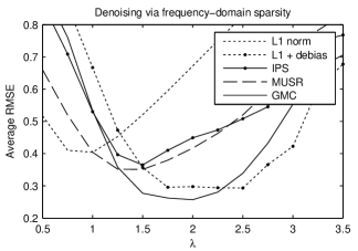
In this denoising experiment, we use 20 realizations of the noise. Each method calls for a regularization parameter λ𝜆{\lambda} to be set. We vary λ𝜆{\lambda} from 0.5 to 3.5 (with increment 0.25) and evaluate the RMSE for each method, for each λ𝜆{\lambda}, and for each realization. For the GMC method we must also specify the matrix B𝐵B, which we set using (48) with γ=0.8𝛾0.8\gamma=0.8. Since B𝖧Bsuperscript𝐵𝖧𝐵B^{\mathsf{H}}\!B is not diagonal, the GMC penalty is non-separable. The average RMSE as a function of λ𝜆{\lambda} for each method is shown in Fig. 11.

The GMC compares favorably with the other methods, achieving the minimum average RMSE. The next best-performing method is debiasing of the 1subscript1\ell_{1}-norm solution, which performs almost as well as GMC. Note that this debiasing method does not minimize an initially prescribed cost function, in contrast to the other methods. The IPS algorithm aims to minimize a (non-convex) cost function.

Figure 10 shows the 1subscript1\ell_{1}-norm and GMC solutions for a particular noise realization. The solutions shown in this figure were obtained using the value of λ𝜆{\lambda} that minimizes the average RMSE (λ=1.0𝜆1.0{\lambda}=1.0 and λ=2.0𝜆2.0{\lambda}=2.0, respectively). Comparing the 1subscript1\ell_{1} norm and GMC solutions, we observe: the GMC solution is more sparse in the frequency domain; and the 1subscript1\ell_{1} norm solution underestimates the coefficient amplitudes.

Neither increasing nor decreasing the regularization parameter λ𝜆{\lambda} helps the 1subscript1\ell_{1}-norm solution here. A larger value of λ𝜆{\lambda} makes the 1subscript1\ell_{1}-norm solution sparser, but reduces the coefficient amplitudes. A smaller value of λ𝜆{\lambda} increases the coefficient amplitudes of the 1subscript1\ell_{1}-norm solution, but makes the solution less sparse and more noisy.

Note that the purpose of this example is to compare the proposed GMC penalty with other sparse regularizers. We are not advocating it for frequency estimation per se.
Refer to caption
Figure 11: Average RMSE for three denoising methods.

8.2 Denoising using time-frequency sparsity

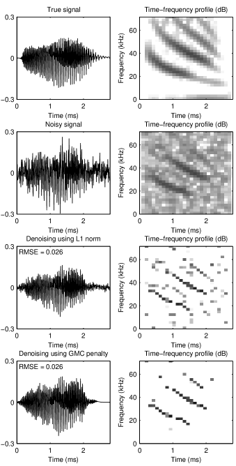
This example considers the denoising of a bat echolocation pulse, shown in Fig. 12 (sampling period of 7 microseconds).111The bat echolocation pulse data is curtesy of Curtis Condon, Ken White, and Al Feng of the Beckman Center at the University of Illinois. Available online at http://dsp.rice.edu/software/bat-echolocation-chirp. The bat pulse can be modeled as sparse in the time-frequency domain. We use a short-time Fourier transform (STFT) with 75% overlapping segments (the transform is four-times overcomplete). We implement the STFT as a normalized tight frame, i.e., AA𝖧=I𝐴superscript𝐴𝖧𝐼AA^{\mathsf{H}}=I. The bat pulse and its spectrogram are illustrated in Fig. 12. For the denoising experiment, we contaminate the pulse with AWGN (σ=0.05𝜎0.05\sigma=0.05).

Refer to caption
Figure 12: Denoising a bat echolocation pulse using the 1subscript1\ell_{1} norm and GMC penalty. The GMC penalty results in fewer extraneous noise artifacts in the time-frequency representation.

We perform denoising by estimating the STFT coefficients by minimizing the cost function F𝐹F in (46) where A𝐴A represents the inverse STFT operator. We set λ𝜆{\lambda} so as to minimize the root-mean-square error (RMSE). This leads to the values λ=0.030𝜆0.030{\lambda}=0.030 and λ=0.51𝜆0.51{\lambda}=0.51 for the 1subscript1\ell_{1}-norm and GMC penalties, respectively. For the GMC penalty, we set B𝐵B as in (48) with γ=0.7𝛾0.7\gamma=0.7. Since B𝖧Bsuperscript𝐵𝖧𝐵B^{\mathsf{H}}\!B is not diagonal, the GMC penalty is non-separable. We then estimate the bat pulse by computing the inverse STFT of the optimized coefficients. With λ𝜆{\lambda} individually set for each method, the resulting RMSE is about the same (0.026). The optimized STFT coefficients (time-frequency representation) for each solution is shown in Fig. 12. We observe that the GMC solution has substantially fewer extraneous noise artifacts in the time-frequency representation, compared to the 1subscript1\ell_{1} norm solution. (The time-frequency representations in Fig. 12 are shown in decibels with 0 dB being black and -50 dB being white.)

8.3 Sparsity-assisted signal smoothing

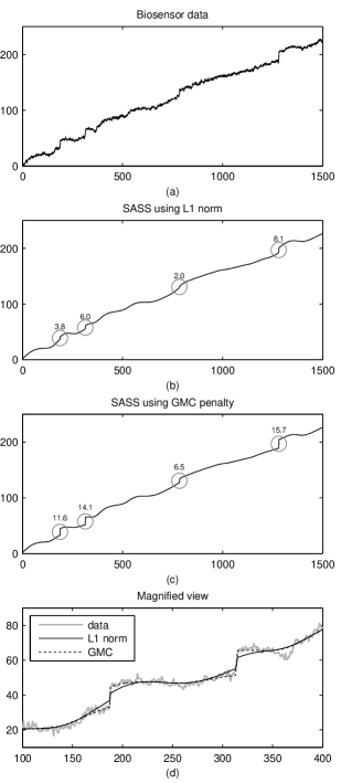
This example uses the GMC penalty for sparsity-assisted signal smoothing (SASS) [53, 50]. The SASS method is suitable for the denoising of signals that are smooth for the exception of singularities. Here, we use SASS to denoise the biosensor data illustrated in Fig. 13(a), which exhibits jump discontinuities. This data was acquired using a whispering gallery mode (WGM) sensor designed to detect nano-particles with high sensitivity [21, 3]. Nano-particles show up as jump discontinuities in the data.

The SASS technique formulates the denoising problem as a sparse deconvolution problem. The cost function to be minimized has the form (46). The exact cost function, given by equation (42) in Ref. [50], depends on a prescribed low-pass filter and the order of the singularities the signal is assumed to posses. For the biosensor data shown in Fig. 13, the singularities are of order K=1𝐾1K=1 since the first-order derivative of the signal exhibits impulses. In this example, we use a low-pass filter of order d=2𝑑2d=2 and cut-off frequency fc=0.01subscript𝑓𝑐0.01f_{c}=0.01 (these parameter values designate a low-pass filter as described in [50]). We set λ=32𝜆32{\lambda}=32 and, for the GMC penalty, we set γ=0.7𝛾0.7\gamma=0.7. Solving the SASS problem using the 1subscript1\ell_{1} norm and GMC penalty yields the denoised signals shown in Figs. 13(b) and 13(c), respectively. The amplitudes of the jump discontinuities are indicated in the figure.
Refer to caption
Figure 13: Sparsity-assisted signal smoothing (SASS) using 1subscript1\ell_{1}-norm and GMC regularization, as applied to biosensor data. The GMC method more accurately estimates jump discontinuities.

It can be seen, especially in Fig. 13(d), that the GMC solution estimates the jump discontinuities more accurately than the 1subscript1\ell_{1} norm solution. The 1subscript1\ell_{1} norm solution tends to underestimate the amplitudes of the jump discontinuities. To reduce this tendency, a smaller value of λ𝜆{\lambda} could be used, but that tends to produce false discontinuities (false detections).

9 Conclusion

In regards to the sparse-regularized linear least squares problem, this work bridges the convex (i.e., 1subscript1\ell_{1} norm) and the non-convex (e.g., psubscript𝑝\ell_{p} norm with p<1𝑝1p<1) approaches, which are usually mutually exclusive and incompatible. Specifically, this work formulates the sparse-regularized linear least squares problem using a non-convex generalization of the 1subscript1\ell_{1} norm that preserves the convexity of the cost function to be minimized. The proposed method leads to optimization problems with no extraneous suboptimal local minima and allows the leveraging of globally convergent, computationally efficient, scalable convex optimization algorithms. The advantage compared to 1subscript1\ell_{1} norm regularization is (i) more accurate estimation of high-amplitude components of sparse solutions or (ii) a higher level of sparsity in a sparse approximation problem. The sparse regularizer is expressed as the 1subscript1\ell_{1} norm minus a smooth convex function defined via infimal convolution. In the scalar case, the method reduces to firm thresholding (a generalization of soft thresholding).

Several extensions of this method are of interest. For example, the idea may admit extension to more general convex regularizers such as total variation [48], nuclear norm [10], mixed norms [34], composite regularizers [2, 1], co-sparse regularization [40], and more generally, atomic norms [14], and partly smooth regularizers [61]. Another extension of interest is to problems where the data fidelity term is not quadratic (e.g., Poisson denoising [24]).

References

  • [1] M. V. Afonso, J. M. Bioucas-Dias, and M. A. T. Figueiredo. An augmented Lagrangian approach to linear inverse problems with compound regularization. In Proc. IEEE Int. Conf. Image Processing (ICIP), pages 4169–4172, September 2010.
  • [2] R. Ahmad and P. Schniter. Iteratively reweighted L1 approaches to sparse composite regularization. IEEE Trans. Comput. Imaging, 1(4):220–235, 2015.
  • [3] S. Arnold, M. Khoshima, I. Teraoka, S. Holler, and F. Vollmer. Shift of whispering-gallery modes in microspheres by protein adsorption. Opt. Lett, 28(4):272–274, February 15, 2003.
  • [4] H. H. Bauschke and P. L. Combettes. Convex Analysis and Monotone Operator Theory in Hilbert Spaces. Springer, 2011.
  • [5] İ. Bayram. Penalty functions derived from monotone mappings. IEEE Signal Processing Letters, 22(3):265–269, March 2015.
  • [6] I. Bayram. On the convergence of the iterative shrinkage/thresholding algorithm with a weakly convex penalty. IEEE Trans. Signal Process., 64(6):1597–1608, March 2016.
  • [7] A. Blake and A. Zisserman. Visual Reconstruction. MIT Press, 1987.
  • [8] S. Boyd and L. Vandenberghe. Convex Optimization. Cambridge University Press, 2004.
  • [9] A. Bruckstein, D. Donoho, and M. Elad. From sparse solutions of systems of equations to sparse modeling of signals and images. SIAM Review, 51(1):34–81, 2009.
  • [10] E. J. Candes and Y. Plan. Matrix completion with noise. Proc. IEEE, 98(6):925–936, June 2010.
  • [11] E. J. Candès, M. B. Wakin, and S. Boyd. Enhancing sparsity by reweighted l1 minimization. J. Fourier Anal. Appl., 14(5):877–905, December 2008.
  • [12] M. Carlsson. On convexification/optimization of functionals including an l2-misfit term. https://arxiv.org/abs/1609.09378, September 2016.
  • [13] M. Castella and J.-C. Pesquet. Optimization of a Geman-McClure like criterion for sparse signal deconvolution. In IEEE Int. Workshop Comput. Adv. Multi-Sensor Adaptive Proc. (CAMSAP), pages 309–312, December 2015.
  • [14] V. Chandrasekaran, B. Recht, P. A. Parrilo, and A. S. Willsky. The convex geometry of linear inverse problems. Foundations of Computational mathematics, 12(6):805–849, 2012.
  • [15] R. Chartrand. Shrinkage mappings and their induced penalty functions. In Proc. IEEE Int. Conf. Acoust., Speech, Signal Processing (ICASSP), pages 1026–1029, May 2014.
  • [16] L. Chen and Y. Gu. The convergence guarantees of a non-convex approach for sparse recovery. IEEE Trans. Signal Process., 62(15):3754–3767, August 2014.
  • [17] P.-Y. Chen and I. W. Selesnick. Group-sparse signal denoising: Non-convex regularization, convex optimization. IEEE Trans. Signal Process., 62(13):3464–3478, July 2014.
  • [18] S. Chen, D. L. Donoho, and M. A. Saunders. Atomic decomposition by basis pursuit. SIAM J. Sci. Comput., 20(1):33–61, 1998.
  • [19] E. Chouzenoux, A. Jezierska, J. Pesquet, and H. Talbot. A majorize-minimize subspace approach for 20subscript2subscript0\ell_{2}-\ell_{0} image regularization. SIAM J. Imag. Sci., 6(1):563–591, 2013.
  • [20] P. L. Combettes. Perspective functions: Properties, constructions, and examples. Set-Valued and Variational Analysis, pages 1–18, 2017.
  • [21] V. R. Dantham, S. Holler, V. Kolchenko, Z. Wan, and S. Arnold. Taking whispering gallery-mode single virus detection and sizing to the limit. Appl. Phys. Lett., 101(4), 2012.
  • [22] I. Daubechies, M. Defrise, and C. De Mol. An iterative thresholding algorithm for linear inverse problems with a sparsity constraint. Commun. Pure Appl. Math, 57(11):1413–1457, 2004.
  • [23] Y. Ding and I. W. Selesnick. Artifact-free wavelet denoising: Non-convex sparse regularization, convex optimization. IEEE Signal Processing Letters, 22(9):1364–1368, September 2015.
  • [24] F.-X. Dupé, J. M. Fadili, and J.-L. Starck. A proximal iteration for deconvolving Poisson noisy images using sparse representations. IEEE Trans. Image Process., 18(2):310–321, 2009.
  • [25] J. Fan and R. Li. Variable selection via nonconcave penalized likelihood and its oracle properties. J. Amer. Statist. Assoc., 96(456):1348–1360, 2001.
  • [26] M. Figueiredo and R. Nowak. An EM algorithm for wavelet-based image restoration. IEEE Trans. Image Process., 12(8):906–916, August 2003.
  • [27] M. A. T. Figueiredo, R. D. Nowak, and S. J. Wright. Gradient projection for sparse reconstruction: Application to compressed sensing and other inverse problems. IEEE J. Sel. Top. Signal Process., 1(4):586–598, December 2007.
  • [28] M. Fornasier and H. Rauhut. Iterative thresholding algorithms. J. of Appl. and Comp. Harm. Analysis, 25(2):187–208, 2008.
  • [29] H.-Y. Gao and A. G. Bruce. Waveshrink with firm shrinkage. Statistica Sinica, 7:855–874, 1997.
  • [30] G. Gasso, A. Rakotomamonjy, and S. Canu. Recovering sparse signals with a certain family of nonconvex penalties and DC programming. IEEE Trans. Signal Process., 57(12):4686–4698, December 2009.
  • [31] A. Gholami and S. M. Hosseini. A general framework for sparsity-based denoising and inversion. IEEE Trans. Signal Process., 59(11):5202–5211, November 2011.
  • [32] W. He, Y. Ding, Y. Zi, and I. W. Selesnick. Sparsity-based algorithm for detecting faults in rotating machines. Mechanical Systems and Signal Processing, 72-73:46–64, May 2016.
  • [33] P. J. Huber. Robust estimation of a location parameter. The Annals of Mathematical Statistics, 35(1):73–101, 1964.
  • [34] M. Kowalski and B. Torrésani. Sparsity and persistence: mixed norms provide simple signal models with dependent coefficients. Signal, Image and Video Processing, 3(3):251–264, 2009.
  • [35] A. Lanza, S. Morigi, I. Selesnick, and F. Sgallari. Nonconvex nonsmooth optimization via convex–nonconvex majorization–minimization. Numerische Mathematik, 136(2):343–381, 2017.
  • [36] A. Lanza, S. Morigi, and F. Sgallari. Convex image denoising via non-convex regularization with parameter selection. J. Math. Imaging and Vision, 56(2):195–220, 2016.
  • [37] M. Malek-Mohammadi, C. R. Rojas, and B. Wahlberg. A class of nonconvex penalties preserving overall convexity in optimization-based mean filtering. IEEE Trans. Signal Process., 64(24):6650–6664, December 2016.
  • [38] Y. Marnissi, A. Benazza-Benyahia, E. Chouzenoux, and J.-C. Pesquet. Generalized multivariate exponential power prior for wavelet-based multichannel image restoration. In Proc. IEEE Int. Conf. Image Processing (ICIP), 2013.
  • [39] H. Mohimani, M. Babaie-Zadeh, and C. Jutten. A fast approach for overcomplete sparse decomposition based on smoothed l0 norm. IEEE Trans. Signal Process., 57(1):289–301, January 2009.
  • [40] S. Nam, M. E. Davies, M. Elad, and R. Gribonval. The cosparse analysis model and algorithms. J. of Appl. and Comp. Harm. Analysis, 34(1):30–56, 2013.
  • [41] M. Nikolova. Estimation of binary images by minimizing convex criteria. In Proc. IEEE Int. Conf. Image Processing (ICIP), pages 108–112 vol. 2, 1998.
  • [42] M. Nikolova. Markovian reconstruction using a GNC approach. IEEE Trans. Image Process., 8(9):1204–1220, 1999.
  • [43] M. Nikolova. Energy minimization methods. In O. Scherzer, editor, Handbook of Mathematical Methods in Imaging, chapter 5, pages 138–186. Springer, 2011.
  • [44] M. Nikolova, M. K. Ng, and C.-P. Tam. Fast nonconvex nonsmooth minimization methods for image restoration and reconstruction. IEEE Trans. Image Process., 19(12):3073–3088, December 2010.
  • [45] A. Parekh and I. W. Selesnick. Enhanced low-rank matrix approximation. IEEE Signal Processing Letters, 23(4):493–497, April 2016.
  • [46] N. Parikh and S. Boyd. Proximal algorithms. Foundations and Trends in Optimization, 1(3):123–231, 2014.
  • [47] J. Portilla and L. Mancera. L0-based sparse approximation: two alternative methods and some applications. In Proceedings of SPIE, volume 6701 (Wavelets XII), San Diego, CA, USA, 2007.
  • [48] L. Rudin, S. Osher, and E. Fatemi. Nonlinear total variation based noise removal algorithms. Physica D, 60:259–268, 1992.
  • [49] I. Selesnick. Sparsity amplified. In Proc. IEEE Int. Conf. Acoust., Speech, Signal Processing (ICASSP), pages 4356–4360, March 2017.
  • [50] I. Selesnick. Sparsity-assisted signal smoothing (revisited). In Proc. IEEE Int. Conf. Acoust., Speech, Signal Processing (ICASSP), pages 4546–4550, March 2017.
  • [51] I. Selesnick. Total variation denoising via the Moreau envelope. IEEE Signal Processing Letters, 24(2):216–220, February 2017.
  • [52] I. Selesnick and M. Farshchian. Sparse signal approximation via nonseparable regularization. IEEE Trans. Signal Process., 65(10):2561–2575, May 2017.
  • [53] I. W. Selesnick. Sparsity-assisted signal smoothing. In R. Balan et al., editors, Excursions in Harmonic Analysis, Volume 4, pages 149–176. Birkhäuser Basel, 2015.
  • [54] I. W. Selesnick and I. Bayram. Sparse signal estimation by maximally sparse convex optimization. IEEE Trans. Signal Process., 62(5):1078–1092, March 2014.
  • [55] I. W. Selesnick and I. Bayram. Enhanced sparsity by non-separable regularization. IEEE Trans. Signal Process., 64(9):2298–2313, May 2016.
  • [56] I. W. Selesnick, A. Parekh, and I. Bayram. Convex 1-D total variation denoising with non-convex regularization. IEEE Signal Processing Letters, 22(2):141–144, February 2015.
  • [57] E. Soubies, L. Blanc-Féraud, and G. Aubert. A continuous exact 0subscript0\ell_{0} penalty (CEL0) for least squares regularized problem. SIAM J. Imag. Sci., 8(3):1607–1639, 2015.
  • [58] C. Soussen, J. Idier, J. Duan, and D. Brie. Homotopy based algorithms for 0subscript0\ell_{0}-regularized least-squares. IEEE Trans. Signal Process., 63(13):3301–3316, July 2015.
  • [59] J.-L. Starck, F. Murtagh, and J. Fadili. Sparse image and signal processing: Wavelets and related geometric multiscale analysis. Cambridge University Press, 2015.
  • [60] M. E. Tipping. Sparse Bayesian learning and the relevance vector machine. J. Machine Learning Research, 1:211–244, 2001.
  • [61] S. Vaiter, C. Deledalle, J. Fadili, G. Peyré, and C. Dossal. The degrees of freedom of partly smooth regularizers. Annals of the Institute of Statistical Mathematics, pages 1–42, 2016.
  • [62] S. Voronin and R. Chartrand. A new generalized thresholding algorithm for inverse problems with sparsity constraints. In Proc. IEEE Int. Conf. Acoust., Speech, Signal Processing (ICASSP), pages 1636–1640, May 2013.
  • [63] D. P. Wipf, B. D. Rao, and S. Nagarajan. Latent variable Bayesian models for promoting sparsity. IEEE Trans. Inform. Theory, 57(9):6236–6255, September 2011.
  • [64] J. Woodworth and R. Chartrand. Compressed sensing recovery via nonconvex shrinkage penalties. Inverse Problems, 32(7):75004–75028, July 2016.
  • [65] C.-H. Zhang. Nearly unbiased variable selection under minimax concave penalty. The Annals of Statistics, pages 894–942, 2010.
  • [66] H. Zou and R. Li. One-step sparse estimates in nonconcave penalized likelihood models. Ann. Statist., 36(4):1509–1533, 2008.