Authors’ Instructions
Predicting Crime Using Spatial Features
Abstract
Our study aims to build a machine learning model for crime prediction using geospatial features for different categories of crime. The reverse geocoding technique is applied to retrieve open street map (OSM) spatial data. This study also proposes finding extracted from crime area found by Hierarchical Density-Based Spatial Clustering of Applications with Noise (HDBSCAN). A spatial distance feature is then computed based on the position of different for various types of crime and this value is used as a feature for classifiers. We test the engineered features in crime data from Royal Canadian Mounted Police of Halifax, NS. We observed a significant performance improvement in crime prediction using the new generated spatial features.
1 Introduction
In recent years, with the availability of high volume of crime data, scientists have been motivated to pursue research in the field of crime and criminal investigations. Understanding the factors related to different categories of crimes and their consequences is particularly essential. The study shown in [7] applies the procedure of statistical analysis on violent crime, poverty, and income inequality and outlines that homicide and assault has more connection and correlation with poverty or income inequality than other crimes. The research found that crime in the real-world highly correlates with time, place and population which make the researcher’s task more complicated [3]. Moreover, this geographical and demographic information contain many discriminatory decision pattern [10, 6]. Leveraging data mining and machine learning techniques with crime research offer the analysts the possibility of better analysis and crime prediction, as well as mining association rules for crime pattern detection.
Our study aims to build a machine learning model to predict the relationship between criminal activity and geographical regions. We choose Nova Scotia (NS) crime data as the target of our study. We focus on four different categories of crime: (i) alcohol-related; (ii) assault; (iii) property crime; and (iv) motor vehicle. In this work, we focus on the creation of two spatial features to predict crime: (i) gecoding; (ii) crime .
The contributions of this work include how geocoding can be used to create features using OSM data and crime are created using a density-based clustering algorithm. Moreover, are extracted from the . We show using a real-world scenario that these two new features increase the performance of different classifiers for predicting four different types of crime.
2 Related Work
The existing work on crime prediction can be categorized into three different groups based on the features such as temporal, spatial and demographic aspects.
Bromley and Nelson [1] reveal temporal patterns of crime to predict alcohol-related crime in Worcester city. They also provide valuable insight into the spatial characteristics of the alcohol-related crime. The authors examine the patterns of crime and disorder at street level by identifying . Ratcliffe [11] proposes three types of temporal and spatial for crime pattern detection. The author also shows how the spatial and temporal characteristics combine through his matrix. However, the author did not apply any machine learning strategy to predict crime.
In [2], the authors analyze four categories of crime data which include liquor law violations, assaults and batteries, vandalism, and noise complaints. Different categories of crime show different temporal patterns. Brower and Carroll [2] clarify crime movement through the city of Madison using GIS mapping. The authors investigate the relationships among high-density alcohol outlets and different neighborhoods. Chainey et al. [5] identify crime using Kernel Density Estimation (KDE) to predict spatial crime patterns. Similarly, in another study, Nakaya and Yano [8] create crime with the help of KDE. However, they combine temporal features with crime analysis.
Nath [9] employed a semi-supervised clustering technique for detecting crime patterns. In [13], the authors propose a pattern detection algorithm named Series Finder to detect patterns of a crime automatically. In [12], the authors study crime rate inference problem using Point-Of-Interest data and taxi flow data. Point-Of-Interest data and taxi flow data are used to enhance the demographic information and the geographical proximity correlation respectively.
None of these features reported in the section were used for predicting crime categories alongside crime pattern detection. In our research, we mainly focus on the spatial aspect of crime prediction. We use geocoding technique and crime to generate new features.
3 Engineering Spatial Features
Geocoding is the process of spatial representation of a location by transforming descriptive information such as coordinates, postal address, and place name. The geocoding process relies on GIS and record linkage of address points, street network and boundaries of administrative unit or region. For this work, we used geocoding to extract the spatial information from the crime data. The geocoder library written in Python, was used for geocoding services with the Open Street Map (OSM) provider. The output of the Geocoder package can be 108 types of location including pubs, bus stops, or hospitals from NS. According to OSM documentation, all of these types are grouped into 12 categories including amenity, shop, office etc. We used both types of location and category as features to predict crime.
The second type of feature used in this work was the creation of . analysis can emphasize the patterns of data regarding time and location of a geographic area. For a crime analyst, the creation of became very popular to identify high concentrated crime area. In this work, are created and transformed into a feature to predict different crime types. The idea is to cluster crime data into regions with a high rate of occurrence of the same crime type. We decided to use HDBSCAN [4] because of its complexity (O()) and because it can handle data with variable density and eliminates the () parameter of DBSCAN which determines the distance threshold to cluster data. In this work, we used the Haversine distance in both HDBSCAN and shortest distance to a . The haversine formula determines the shortest distance between two points on earth located by their latitudes and longitudes.
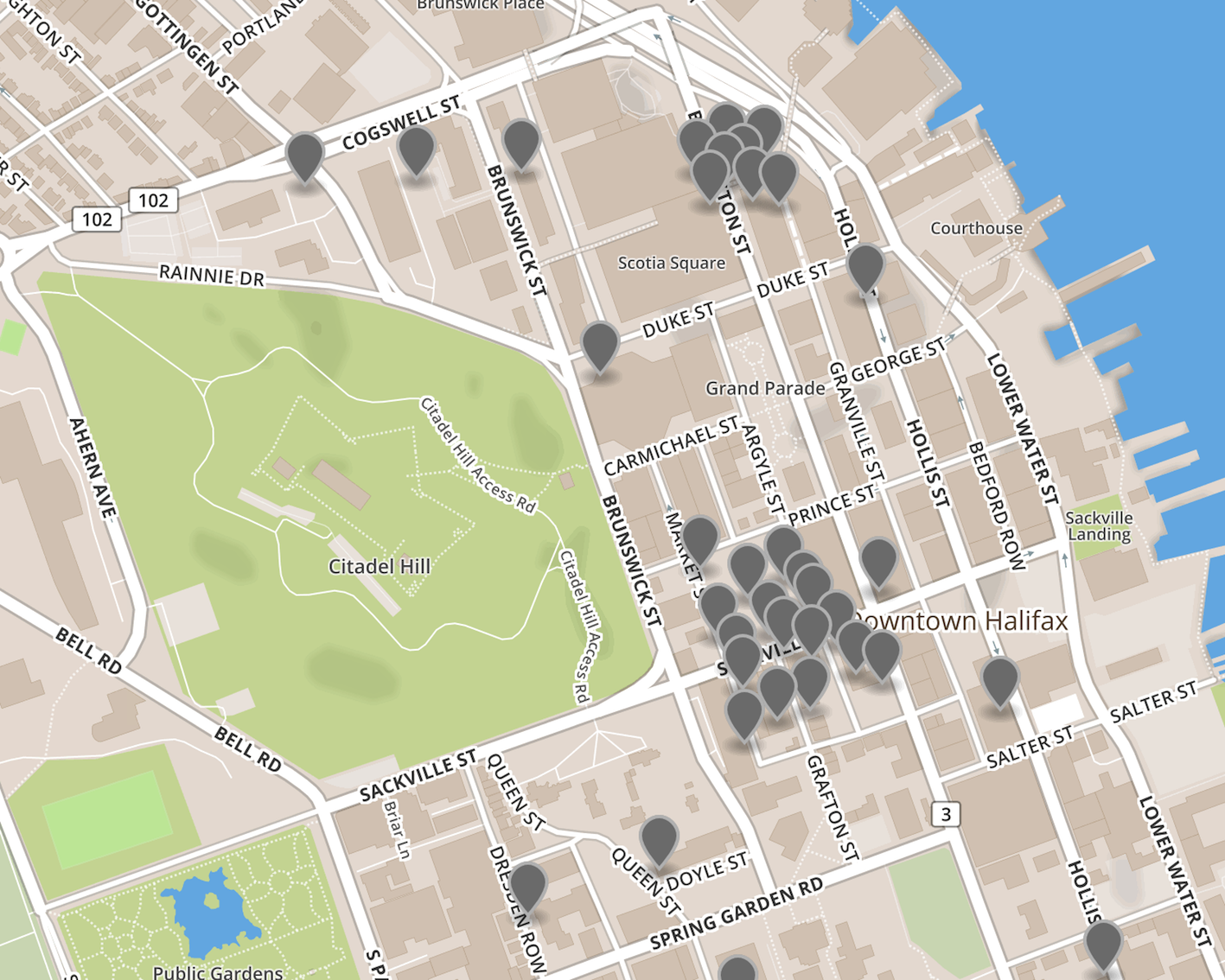
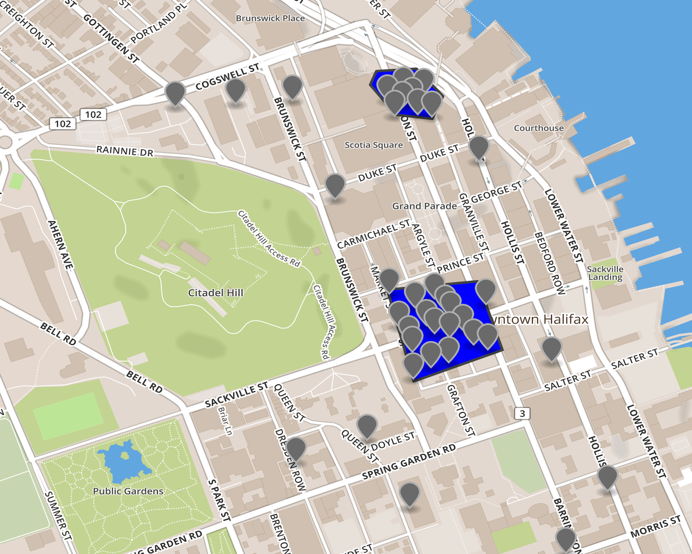
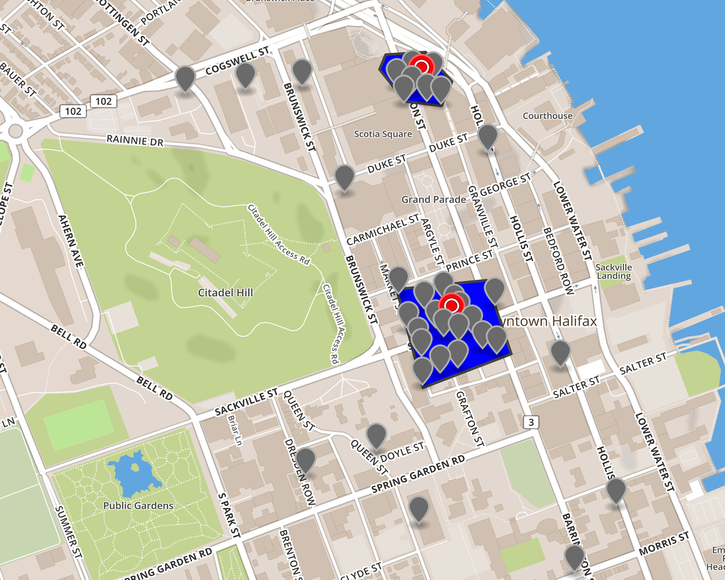
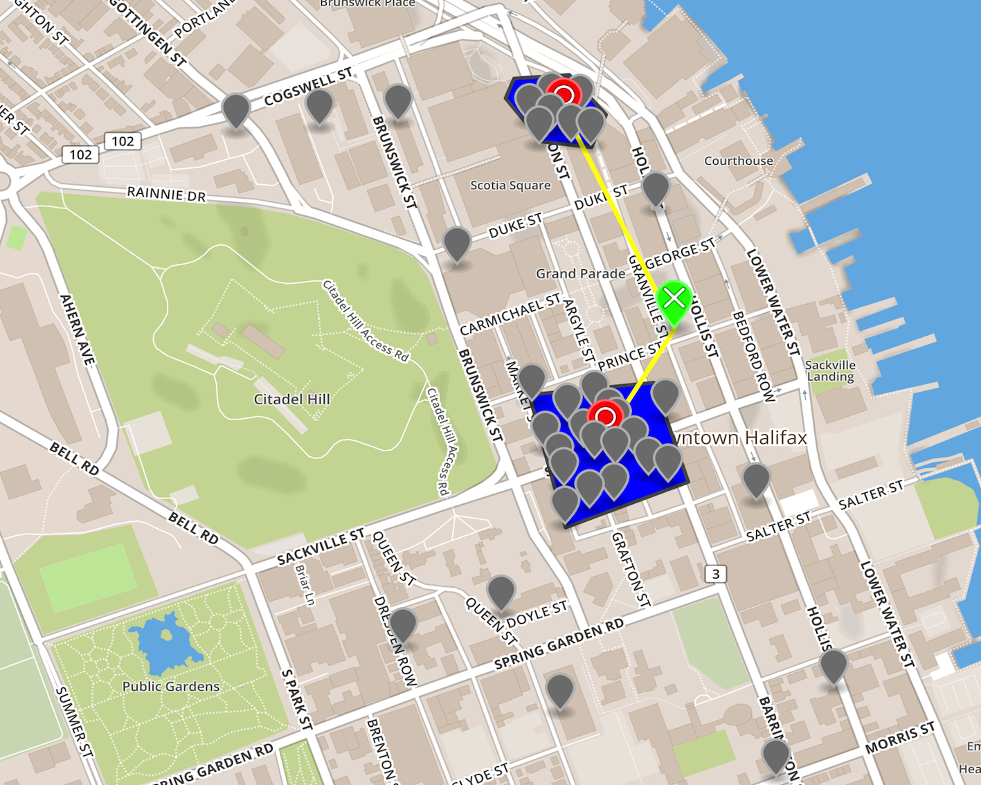
Figure 2(d) summarizes the overall process to produce the shortest distance for feature. Figure 2(d) (a) shows crime examples (gray pins) in downtown Halifax area. Then, a (blue area) found by HDBSCAN is shown in Figure 2(d) (b). Figure 2(d) (c) shows a (red pin) extracted from a . Finally, a new crime example (green pin) is evaluated, and the distances to (yellow line) are calculated. The feature used in this work will select the shortest distance to a as a feature for classifying a crime type.


4 Experiments
This section outlines the experiments performed in this work and reports the experimental results obtained by the proposed classifiers trained on all raw features and the engineered spatial features.
Crime data from Halifax regional police department are used in this work, and it covers most of the districts in Nova Scotia province in Canada. For our experiments, we explore all of the offenses of 2016 which include 3726 data samples. The crime attributes extracted from the source data include geographic location, incident_start_time, month, weekday, ucr_descriptions, and whether the incident happened because of alcohol.
We also group our data using four different classes, named alcohol-related, assault, property damage, and motor vehicle using the ucr_descriptions and alcohol incident fields. For the alcohol-related crimes, we considered all the cases where alcohol presence was reported in the UCR using the alcohol incident field (53% alcohol, 47% no alcohol). For all the remaining classes, the ucr_description field was used. The assault group (65% assault, 35% no assault) covers all levels of assault including sexual assault, aggravated assault, bodily harm, threat, etc. Property damage group covers break, theft, robbery, etc (65% property damage, 35% no property damage). Motor vehicle group covers all types of motor vehicle accident, act violation and impair driving (65% motor vehicle, 35% no motor vehicle).
To create the shortest distance to a , we used UCR form data from the year of 2015. We created for each positive class and the respective shortest distance to a was used in the experiment.
The classifiers used in this work are Logistic Regression (LR), Support Vector Machine (SVM), and Random Forest (RF) and an Ensemble with all the previous classifiers. We evaluate the classifiers’ performance using the accuracy and Area Under the Curve (AUC) of the ROC (Receiving Operator Characteristic) analysis. The baseline used in this work to verify if the newly engineered features help a classifier to improve the crime prediction power was the raw data contained in the UCR form (incident_start_time, month, and weekday). A 10-fold cross-validation was used in all phases to estimate model prediction performance correctly and paired t-tests (significance level of 0.05) were used to test the statistical difference significance of raw and engineered features.
Table 1 shows the classification accuracy for LR, SVM, RF and an ensemble of these methods for all four categories of crime. For each method, the first column displays the accuracy of raw features and the second column for engineered spatial features. The * in Table 1 symbol indicates that the method fails for the statistical hypothesis testing, i.e., the p-value is higher than 0.05.
For the Alcohol-related group, the results show that new spatial features achieve better accuracy in comparison with raw features for all four methods with statistical evidence support, and the Ensemble method performs better than others (75.52% of accuracy) with almost 17% accuracy improvement. The accuracy values of the engineered features for the Assault and Property damage groups shows that all methods, except LR, benefit from their inclusion. For example, adding engineered features with raw features improves nearly 11% (Assault group) and 5% (Property damage group) of accuracy for RF method. Finally, for the Motor vehicle group, all the classifiers showed improvements, except for the Ensemble classifier.
| LR | RF | SVM | Ensemble | |||||
| Crime type | raw | eng. | raw | eng. | raw | eng. | raw | eng. |
| Alcohol-related | 59.36 | 65.27 | 57.73 | 73.51 | 59.28 | 71.31 | 58.61 | 75.52 |
| Assault | 65.35 | 65.03* | 47.94 | 58.89 | 63.53 | 65.27 | 55.96 | 64.41 |
| Property damage | 88.43 | 88.41* | 84.03 | 88.57 | 88.19 | 88.43 | 88.43 | 88.44* |
| Motor vehicle | 81.59 | 82.31 | 71.82 | 81.45 | 81.11 | 81.45 | 81.56 | 81.80* |
Table 2 shows the AUC scores for LR, SVM, RF and an ensemble of LR, SVM & RF methods. For Alcohol-related and Motor vehicle crimes, the results discovered that spatial features give better AUC scores than raw features for all four methods. For instance, the Ensemble method gives 82.5% and 69.4% AUC score for Alcohol-related and Motor vehicle crimes respectively based on engineered features. Similarly, for Assault and Property damage crime, LR, RF and Ensemble methods perform significantly better with engineered features. Adding engineered features with raw features gives 56.7% and 65.7% AUC score for Assault and Property damage crime respectively with the Ensemble method. Therefore, using spatial features, the Ensemble method performs at least 10% improvement in AUC score for all four categories of crime. However, for SVM method, there is no significant evidence of improvement.
| LR | RF | SVM | Ensemble | |||||
| Crime type | raw | eng. | raw | eng. | raw | eng. | raw | eng. |
| Alcohol-related | .575 | .723 | .649 | .818 | .635 | .747 | .661 | .825 |
| Assault | .528 | .613 | .457 | .545 | .504 | .533* | .459 | .567 |
| Property damage | .519 | .651 | .531 | .646 | .501 | .505* | .534 | .657 |
| Motor vehicle | .515 | .686 | .488 | .682 | .494 | .536 | .490 | .694 |
5 Conclusions and Future Work
In this work, we explored the creation of spatial features derived from geolocated data. We created two types of spatial features: (i) geocoding; and (ii) shortest distance to a . The new features were evaluated using four different crime types using only the information provided in the UCR forms as features for a classifier as the baseline. The results show that significant improvements in accuracy and AUC were found when the newly engineered features were added to the tested classifiers.
We intend to extend this work in other directions. As our study focuses on real world datasets, the subject of data discrimination is another important concern. Data discrimination refers to bias that happens because of contradistinction among different data sources. Another research direction we want to explore is the possibility of performing transfer learning from what was learned in NS to other Canadian provinces.
Acknowledgments
The authors would like to thank NSERC, NS Health Authority and Injury Free Nova Scotia for financial and other supports.
References
- [1] Bromley, R.D., Nelson, A.L.: Alcohol-related crime and disorder across urban space and time: evidence from a british city. Geoforum 33(2), 239–254 (2002)
- [2] Brower, A.M., Carroll, L.: Spatial and temporal aspects of alcohol-related crime in a college town. Journal of American College Health 55, 267–275 (2007)
- [3] Buczak, A.L., Gifford, C.M.: Fuzzy association rule mining for community crime pattern discovery. In: ACM SIGKDD Workshop on Intelligence and Security Informatics. pp. 2:1–2:10. ISI-KDD ’10, ACM, New York, NY, USA (2010)
- [4] Campello, R.J.G.B., Moulavi, D., Sander, J.: Density-based clustering based on hierarchical density estimates. In: Advances in Knowledge Discovery and Data Mining. pp. 160–172. Springer Berlin Heidelberg (2013), https://doi.org/10.1007/978-3-642-37456-2_14
- [5] Chainey, S., Tompson, L., Uhlig, S.: The utility of hotspot mapping for predicting spatial patterns of crime. Security Journal 21(1), 4–28 (2008)
- [6] Executive Office of the President: Big Data: A Report on Algorithmic Systems, Opportunity, and Civil Rights. CreateSpace Independent Publishing Platform, 2nd edn. (2016)
- [7] Hsieh, C.C., Pugh, M.D.: Poverty, income inequality, and violent crime: A meta-analysis of recent aggregate data studies. Criminal Justice Review 18(2), 182–202 (1993)
- [8] Nakaya, T., Yano, K.: Visualising crime clusters in a space-time cube: An exploratory data-analysis approach using space-time kernel density estimation and scan statistics. T. GIS 14(3), 223–239 (2010)
- [9] Nath, S.V.: Crime pattern detection using data mining. In: Proceedings of the 2006 IEEE/WIC/ACM International Conference on Web Intelligence and Intelligent Agent Technology. pp. 41–44. WI-IATW ’06, IEEE Computer Society, Washington, DC, USA (2006), http://dx.doi.org/10.1109/WI-IATW.2006.55
- [10] Pedreschi, D., Ruggieri, S., Turini, F.: Measuring discrimination in socially-sensitive decision records. In: Proceedings of the SIAM International Conference on Data Mining, SDM 2009, April 30 - May 2, 2009, Sparks, Nevada, USA. pp. 581–592 (2009)
- [11] Ratcliffe, J.: The hotspot matrix: A framework for the spatio-temporal targeting of crime reduction. Police Practice and Research 5(1), 5–23 (2004)
- [12] Wang, H., Kifer, D., Graif, C., Li, Z.: Crime rate inference with big data. In: Proceedings of the 22nd ACM SIGKDD International Conference on Knowledge Discovery and Data Mining, San Francisco, CA, USA, August 13-17, 2016. pp. 635–644 (2016), http://doi.acm.org/10.1145/2939672.2939736
- [13] Wang, T., Rudin, C., Wagner, D., Sevieri, R.: Learning to detect patterns of crime. In: ECML/PKDD (3). Lecture Notes in Computer Science, vol. 8190, pp. 515–530. Springer (2013)