Cavendish-HEP-2018-06, DAMTP-2018-12,
KCL-PH-TH/2018-12, CERN-PH-TH/2018-042
Updated Global SMEFT Fit to Higgs,
Diboson and Electroweak Data
John Ellisa,b, Christopher W. Murphyc, Verónica Sanzd and Tevong Youe
a Theoretical Particle Physics and Cosmology Group, Department of
Physics, King’s College London, London WC2R 2LS, United Kingdom
b National Institute of Chemical Physics & Biophysics, Rävala 10, 10143 Tallinn, Estonia;
Theoretical Physics Department, CERN, CH-1211 Geneva 23,
Switzerland
c Department of Physics, Brookhaven National Laboratory, Upton, New York, 11973, USA
d Department of Physics and Astronomy, University of Sussex, Brighton BN1 9QH, UK
e DAMTP, University of Cambridge, Wilberforce Road, Cambridge, CB3 0WA, UK;
Cavendish Laboratory, University of Cambridge, J. J. Thomson Avenue, Cambridge, CB3 0HE,
UK
Abstract
The ATLAS and CMS collaborations have recently released significant new data on Higgs and diboson production in LHC Run 2. Measurements of Higgs properties have improved in many channels, while kinematic information for and can now be more accurately incorporated in fits using the STXS method, and diboson production at high gives new sensitivity to deviations from the Standard Model. We have performed an updated global fit to precision electroweak data, measurements at LEP, and Higgs and diboson data from Runs 1 and 2 of the LHC in the framework of the Standard Model Effective Field Theory (SMEFT), allowing all coefficients to vary across the combined dataset, and present the results in both the Warsaw and SILH operator bases. We exhibit the improvement in the constraints on operator coefficients provided by the LHC Run 2 data, and discuss the correlations between them. We also explore the constraints our fit results impose on several models of physics beyond the Standard Model, including models that contribute to the operator coefficients at the tree level and stops in the MSSM that contribute via loops.
March 2018
1 Introduction
In the absence (so far) of any clear signature of some physics beyond the Standard Model (BSM) at the LHC, the Standard Model Effective Field Theory (SMEFT) has emerged as one of the most interesting tools to probe systematically the data from the LHC and elsewhere for hints of possible BSM physics111See Refs. [1, 2, 3, 4] for some recent reviews of the SMEFT.. The formulation of the SMEFT assumes that all the known particles have the same SU(3)SU(2)U(1)Y gauge transformation properties as in the Standard Model Model (SM), with their conventional dimension-2 and -4 interactions being supplemented by higher-dimensional interactions between all allowed combinations of these SM fields. Such interactions might be generated by massive particles being exchanged at the tree-level or circulating in loop diagrams. These interactions would in general be suppressed by powers of some high mass scale related to the scale of BSM physics, with dimensionless coefficients that depend on their interactions with SM particles. The leading higher-dimensional operators relevant to many LHC measurements are expected to be those of dimension 6. If the LHC experiments measure one or more significant deviations from SM predictions, the SMEFT can be used to help characterize its possible origin. In the absence of any significant deviations, the SMEFT can be used to constrain the scales of different BSM physics scenarios and to guide the search for direct effects of new physics.
First steps in this SMEFT programme have included the cataloguing of possible interactions of dimension 5, 6 and higher [5, 6, 7, 8], the construction of non-redundant bases of independent operators [9, 10, 11, 12, 1], and the development of a dictionary to translate between different bases [13, 14]. This groundwork has been the basis for subsequent phenomenological analyses through global fits of data [15, 16, 17, 18, 19, 20, 21, 22, 23, 24, 25, 26, 27, 28, 29, 30, 31, 32, 33, 34, 35, 36, 37, 38, 39, 40] from the LHC and other experiments that constrain various combinations of dimension-6 operator coefficients and thereby different scenarios for BSM physics. The principal classes of observables used in such analyses have included precision electroweak data from LEP [41], the SLC [41] and the Tevatron [42], constraints on diboson production from LEP 2 [43, 44, 45, 46] and the LHC [47, 48], and data on Higgs production from the LHC [49]. In the past, the precision of the electroweak -pole data has been such that the coefficients of the operators affecting them could initially be considered independently of those entering into other observables. However, such a segregated approach is theoretically unsatisfactory, with some bases being more correlated across measurements than others, and is becoming obsolescent with the advent of more precise LHC data on Higgs production and diboson production where the latter, in particular, can no longer be interpreted solely as a measurement of anomalous triple-gauge couplings [50, 51].
In this paper we perform the first comprehensive global analysis of relevant electroweak and diboson data together with Higgs production data from Runs 1 and 2 of the LHC, while allowing all relevant operators to vary in the combined dataset, thus superseding our previous analyses [17, 18, 19]. As we discuss in more detail below, we include in our analysis 14 precision electroweak measurements, 74 measurements of fermions, 22 Higgs signal strength measurements from Run 1 of the LHC and 46 measurements of Higgs production from Run 2 of the LHC (including information using Simplified Template Cross Sections (STXS) [1]), and one measurement of production at high during Run 2 of the LHC.
We present our results in both the Warsaw [9] and SILH [52, 10] operator bases and in two forms: one in which all the dimension-6 operator coefficients are allowed to be non-vanishing simultaneously, and one in which the operator coefficients are switched on one at a time. We exhibit the improvement in the constraints on operator coefficients compared to fits using only data from Run 1 of the LHC, and we discuss the correlations between the constraints on the coefficients. We also analyze the implications of this fit for BSM models that make tree-level contributions to the operator coefficients [53], as well as for stop squarks in the minimal supersymmetric extension of the SM (MSSM), which contribute to the operator coefficients at the loop level [54, 55, 56].
The layout of our paper is as follows. In section 2 we review the SMEFT framework and introduce the 20 dimension-6 operators that appear in our analysis, and in Section 3 we introduce the data we use. Section 4 presents the methodology we use for our fit, and Section 5 presents the results of our analysis. Their implications for a variety of BSM scenarios are discussed in Section 6. Finally, Section 7 summarizes our conclusions.
2 The SMEFT Framework
The SM is defined by a Lagrangian consisting of all operators up to mass dimension 4 formed by combinations of SM fields that are allowed by a linearly-realized SU(3)SU(2)U(1)Y gauge symmetry. However, if new physics exists at some heavier scale , one generically expects higher-dimensional operators to also be present, their effects suppressed by to powers fixed by dimensional analysis, with logarithmic corrections that are calculable in perturbation theory. Treating the SM properly as a low-energy Effective Field Theory (EFT), the SMEFT is the SM Lagrangian extended to include a series of higher-dimensional operators. At dimension 5 there is a single category of operators, which violate lepton number and give masses to neutrinos [5]. Here we focus on the effects of the leading lepton-number-conserving operators of dimension 6,
| (1) |
where the are Wilson coefficients induced by integrating out the heavy degrees of freedom of some new physics at a scale 222For some recent developments on matching using functional methods, see Refs. [54, 57, 58, 59, 60, 61, 62, 63, 64].. One would typically expect a tree-level contribution to be proportional to at least the square of some new physics coupling, e.g., , with an additional suppression by a factor if it appears when the BSM physics is integrated out at one loop. From a bottom-up point of view the coefficients are treated as free parameters where the validity of the EFT can be assessed a posteriori [65].
The coefficients generated at the scale are related to their values at the electroweak scale GeV through RGE running, using the SMEFT one-loop anomalous dimension matrix that has been calculated in Refs. [66, 67, 68, 69, 70, 71, 72]. Below the electroweak scale the SMEFT can be matched to a low-energy EFT [73, 74, 75, 76], whose running is also known [77]. Since the data currently do not require a large hierarchy between the electroweak scale and the BSM scale, and we work to leading order for simplicity333See Refs. [2, 78, 79, 80, 81, 82, 83] for some discussion and results in the SMEFT at NLO., we do not discuss these effects in this paper.
The dimension-6 operators were first classified systematically in Ref. [6]. Such a list generally forms a redundant set since operators related by field redefinitions, equations of motion, integration by parts, or Fierz identities give identical -matrix predictions and are therefore equivalent descriptions of the same physics444The problem of generating a non-redundant set of operators to arbitrary mass dimension has recently been solved using Hilbert series methods [84, 85, 86, 8, 87].. The first non-redundant basis of operators was derived in Ref. [9] and is commonly called the Warsaw basis. Another popular basis in the literature is referred to as the SILH basis [52, 10]. There are 2499 CP-even dimension-6 operators, which reduce to 59 independent operators when assuming minimal flavour violation [71], but of those only 20 are relevant for the Higgs, diboson, and electroweak precision observables that we consider here555We do not consider CP-odd operators in our analysis; for a recent study of CP tests in the Higgs sector see Ref. [88].. We assume here an U(3)5 flavor symmetry, under which the Yukawa matrices are promoted to spurions transforming as bi-triplets, and present results in both the Warsaw and SILH bases.
In the Warsaw basis, the 11 operators involved in diboson measurements and electroweak precision observables, through input parameter shifts or modifications of the gauge boson self-coupling and couplings to fermions, can be written in the notation of Ref. [2] as
| (2) |
where flavour indices and Hermitian conjugate operators are implicit,666 The flavour indices of the four-lepton operator are . and we defined
| (3) |
There are in addition 9 operators that affect Higgs measurements,
| (4) |
The operator, not listed here, can be measured in double-Higgs production, for which there is limited sensitivity at the LHC777Prospects for future double-Higgs measurements at higher luminosity or energy are studied, for example, in Refs. [89, 90, 91, 92, 93, 94, 95] and references therein..
We note that Higgs production in association with a top-quark pair probes many coefficients in the SMEFT [96, 30, 31] but a number of these do not appear in our other observables—the only one we consider explicitly here is , which is expected to make the largest contribution to production. However, it should be borne in mind that the bounds on in this work are actually bounds on the following linear combination of coefficients,
| (5) |
We note also that Higgs production in association with a jet is sensitive to the triple-gluon operator. Although we will sometimes include , or equivalently for the SILH basis, in our fits, more stringent bounds on have been derived from multi-jet processes at the LHC [97]. Other SMEFT operators that do not appear here can be constrained independently of Higgs, diboson, and electroweak precision measurements.
In the SILH basis the relevant operators for our fit, with conventions defined in [10] (which differs slightly from Ref. [98]), are
| (6) |
Hermitian conjugates and flavour indices are again kept implicit.
Our computations are performed at linear order in the Warsaw and SILH bases using , , and as input parameters. We used the predictions for electroweak precision observables and scattering at LEP 2 in the Warsaw basis from Refs. [39, 2]. Predictions for LHC observables are made using [99]. These computations can be converted to the SILH basis using the known results in the literature [71, 54, 13].
3 Data used in the Global Fit
The following data are used in our global fit, which, as stated above, are sensitive to 20 directions in the SMEFT parameter space.
-
•
Precision Electroweak Data: We use the -pole observables from Table 8.5 of Ref. [41], including the correlations. We use the mass measurements from the Tevatron [42] and ATLAS [100]. These measurements and the corresponding theoretical predictions within the SM are summarized in Table 1, and they probe eight directions in the SMEFT.
-
•
: We use all the data from Tables 12, 13, 14, and 15 of Ref. [39]. The original experimental results can be found in Refs. [43, 44, 45, 46], and we use the SM predictions from Ref. [44, 45]. This is a total of 74 measurements. These measurements also probe eight directions in the SMEFT. However only three of these combinations of the parameters are unconstrained by the electroweak precision data.
-
•
Higgs Production in LHC Run 1: We use all the 20 signal strengths from Table 8 of Ref. [49], including the correlations given in Figure 27 of the same paper, where a signal strength is defined as the ratio of the measured cross section to its SM prediction. The ATLAS and CMS combination for the signal strength is taken from Table 13 of Ref. [49]. The ATLAS signal strength is taken from Figure 1 of Ref. [101]. These measurements are summarized in Table 2. The 20 correlated measurements are sensitive to nine combinations of SMEFT parameters, and the measurement of constitutes a tenth direction. However, is a dependent quantity because of the flavor symmetry that we assume.
-
•
Higgs Production in LHC Run 2: We use 25 measurements from CMS [102, 103, 104, 105, 105, 106, 107, 108, 109], and 23 measurements from ATLAS [110, 111, 112, 113, 114, 115, 116]. A summary is given in Table 3. The correlations between the and decay notes from Ref. [115] are also included in the context of template cross sections (STXS) as described in Ref. [117]. These measurements probe 12 combinations of SMEFT parameters888A SMEFT fit to ATLAS Higgs production data is presented in [115]. See also a recent non-linear EFT analysis in [118] and a global SM fit to electroweak and Higgs measurements in [119]..
-
•
Production at the LHC: We use only one measurement of the differential cross section for by ATLAS at 13 TeV [47] as no correlations are provided. The particular bin we chose, which requires the transverse momentum () of the leading lepton () to be greater than 120 GeV, is the overflow bin, which is expected to maximize the sensitivity to certain Wilson coefficients. The signal strength for this measurement is .
| Observable | Measurement | Ref. | SM Prediction | Ref. |
|---|---|---|---|---|
| [GeV] | [41] | [40] | ||
| [nb] | [41] | [40] | ||
| [41] | [40] | |||
| [41] | [120] | |||
| [41] | [120] | |||
| [41] | [120] | |||
| [41] | [40] | |||
| [41] | [40] | |||
| [41] | [120] | |||
| [41] | [120] | |||
| [41] | [120] | |||
| [41] | [120] | |||
| [GeV] | [42] | [120] | ||
| [GeV] | [100] | [120] |
| Production | Decay | Signal Strength | Production | Decay | Signal Strength |
|---|---|---|---|---|---|
| F | |||||
| F | |||||
| F | |||||
| F | |||||
| VBF | |||||
| VBF | |||||
| VBF | |||||
| VBF | |||||
| Production | Decay | Sig. Stren. | Production | Decay | Sig. Stren. | ||
|---|---|---|---|---|---|---|---|
| [102] | 1-jet, | [110] | |||||
| [103] | [111] | ||||||
| [103] | [111] | ||||||
| [104] | [112] | ||||||
| [105] | [113] | ||||||
| [105] | [113] | ||||||
| [105] | [113] | ||||||
| [105] | [113] | ||||||
| [105] | [113] | ||||||
| [105] | [113] | ||||||
| [106] | 0-jet DF | [114] | F | ||||
| [106] | 1-jet DF | [114] | VBF | ||||
| [106] | 2-jet DF | [115] | B B | ||||
| [106] | VBF 2-jet | [115] | 0-jet | ||||
| [106] | 2-jet | [115] | 1-jet, | ||||
| [106] | 3-lep | [115] | 1-jet, | ||||
| [107] | F | [115] | 1-jet, | ||||
| [107] | VBF | [115] | 2-jet | ||||
| [107] | [115] | “BSM-like” | |||||
| [107] | [115] | VBF, | |||||
| [108] | F | [115] | lep | ||||
| [109] | 0-jet | [115] | |||||
| [109] | boosted | [116] | |||||
| [109] | VBF | ||||||
| [106] | 4-lep | ||||||
4 Fit Methodology
We assume Gaussian errors throughout and use the method of least squares to perform our estimation of the SMEFT parameters. The least-squares estimators for the parameters of interest, , are defined by the function
| (7) |
where the measurements tabulated in Section 3 have been collected into a vector of central values, , along with a covariance matrix, . The SMEFT values of the corresponding observables have been expressed as a vector, , where represents the predictions in the SM, is a vector of SMEFT Wilson coefficients, and is a matrix that parameterizes in the linear approximation we use here the SMEFT corrections to the SM predictions.
The least-squares estimators for the Wilson coefficients are found by extremizing the function, :
| (8) |
The covariance matrix for the least-squares estimators, , is given by the inverse of the Hessian of the function, :
| (9) |
The quantity in parentheses in Eq. (9) is also known as the Fisher information. With these definitions an alternative way of writing the chi-squared function is
| (10) |
where is the gradient of the chi-squared function evaluated using the least-squared estimators.
Since our analysis is to linear order in the Wilson coefficients, the likelihood associated with our function is a multivariate Gaussian distribution. As such, it is simple to compute the marginalized likelihood for a given subset of Wilson coefficients. It is not necessary to do any integration, one simply drops the variables the one wants to marginalize over from . We note also that the marginalized and profiled likelihoods for a given subset of Wilson coefficients are equivalent in the Gaussian approximation, which is not true in general.
5 Results
5.1 Oblique Parameters and
As an introduction to the results from our updated global fit, we first present its implications in a simplified case where only the oblique parameters and introduced in [121, 122, 123, 124, 125, 126] are non-zero. In the Warsaw basis these parameters are given by
| (11) |
whereas in the SILH basis the relation (at leading order) is given by and .
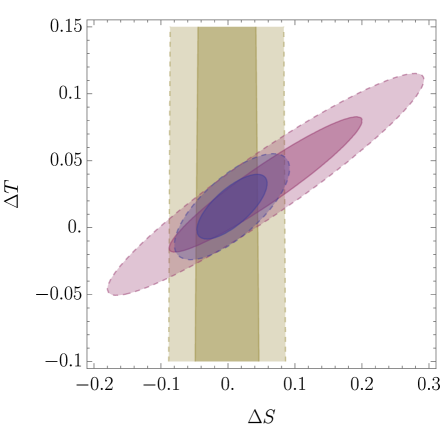
Figure 1 shows the preferred parameter space for and for three different selections of the data sets included in the fit. The green ellipses are obtained using just the -pole, mass, and LEP 2 scattering measurements in the fit, whereas the orange ellipses use only the LHC Run 1 and Run 2 Higgs results. Finally, the blue ellipses are obtained using all the data described in Section 3. The regions shaded in darker and lighter colours are allowed at 1 and 2, respectively. The 2- marginalized ranges of and are
| (12) |
with a correlation coefficient of 0.72.
This two-dimensional fit is restricted to the two operators in the Warsaw basis that contribute to and , as defined by electroweak gauge boson propagator modifications 999These operators also induce vertex corrections that enter in the coupling.. Nevertheless, Figure 1 makes it clear that the importance of the Higgs measurements at the LHC is now comparable to that of the electroweak precision measurements for certain operators, with (basis-dependent) correlations between various measurements. Moreover, these and the Higgs constraints on and are largely complementary in the Warsaw basis [127]. This exemplifies the necessity of performing a combined global fit to precision electroweak, Higgs and diboson data, as we discuss in the rest of this Section.
5.2 Fits to all Operator Coeficients
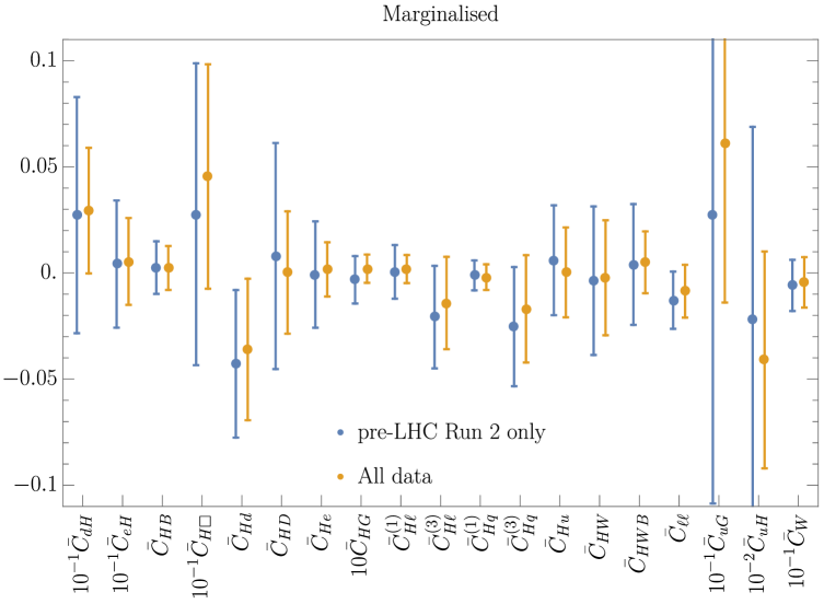
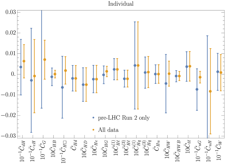
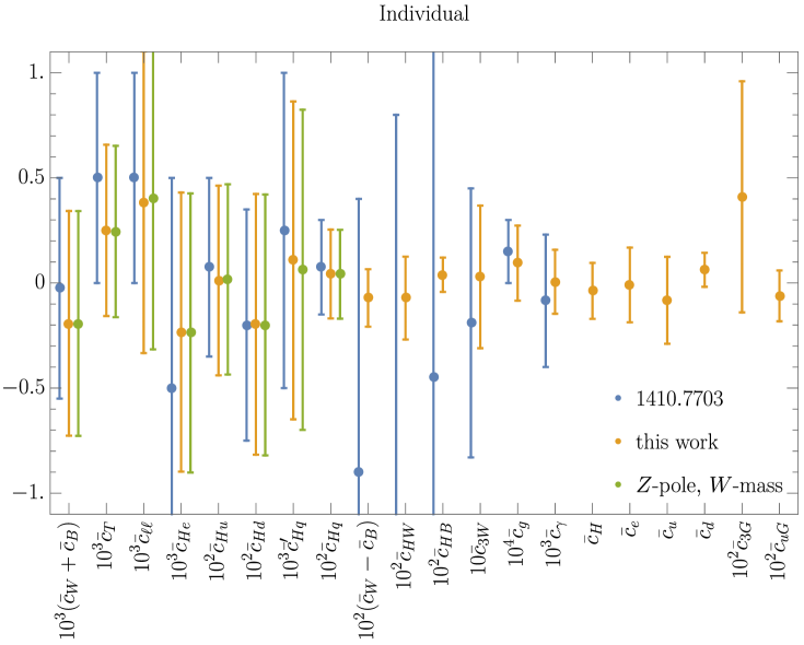
With this motivation, we now turn to the results of our global fit using all the 20 dimension-6 operators discussed previously. The upper panel of Fig. 2 displays our results for the best-fit values and 95% CL ranges in the Warsaw operator basis if all these operators are included simultaneously, while the lower panel shows our results when each operator is turned on individually, with the other operator coefficients set to zero. The orange error bars are for a fit to all the measurements described above, whereas the blue error bars are for a fit omitting the LHC Run 2 data. As one would expect, the uncertainties in each operator coefficient are smaller in the fit including LHC Run 2 data, and are generally larger in the global fit with all operators switched on than in the fit where the operators are switched on one at a time. The numerical results of the global fit for the 1- ranges in the Warsaw basis including all sources of data are presented in the left part of Table 4.
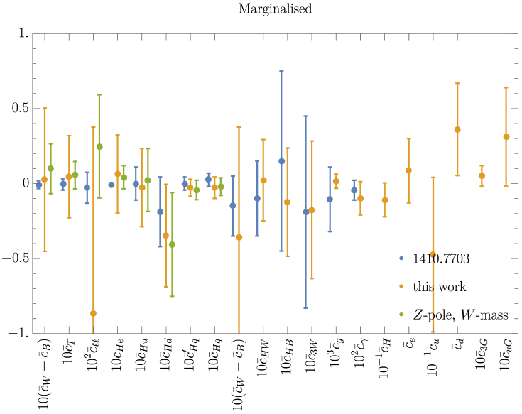
Fig. 3 shows the corresponding best-fit values and 95% CL ranges in the SILH basis. The orange error bars are again for a fit to all the measurements described above, whereas the green error bars are for a fit to the -pole and mass measurements alone. Again, the uncertainties in each operator coefficient are smaller when the LHC Run 2 data are included in the fit, and are generally larger when all operators are switched on simultaneously. The numerical results for the 1- ranges in the global fit to all the available data in the SILH basis are shown in the right part of Table 4.
Fig. 3 also compares the results of the updated global fit performed in this work with those found in previous work in the SILH basis by three of us (JE, VS and TY) in Ref. [18]. It should be borne in mind, when comparing the fits to see how the bounds on different coefficients have changed, that the procedures of the two works are not identical. Nevertheless several general trends can be seen. When considering fits to one operator at a time, the bounds on coefficients that primarily affect - and -pole observables have not changed drastically between Ref. [18] and this work. On the other hand, the bounds in the individual fits on the coefficients of operators that do not affect the electroweak pole observables have tightened, quite considerably in some cases. When all the operators are considered simultaneously there are not such large differences between the bounds on the operators that do not affect - and - pole observables as in the one-at-a-time case.
We show in Table 5 the relative information contents of the different sets of data for the different Wilson coefficients in the Warsaw basis. A cross indicates no current sensitivity. As discussed in, e.g., Ref [18], one can divide sets of operators in terms of their sensitivity to LEP or LHC observables. Operators involving light fermions in the Warsaw basis had been best constrained by LEP -pole and constraints. The introduction of LEP data brings marginal gains, except for the operator where the effect is quite dramatic. For this operator the high-energy LHC data do not yet improve substantially the sensitivity, although one would expect this to change as more statistics are gathered and the complete information in the full distribution is available, not just the overflow bin.
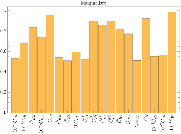
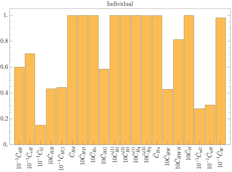
The LHC Run 1 data opened the possibility to explore a new set of operators involving the Higgs and gauge bosons to which LEP was not sensitive. For all these operators, the Run 2 dataset is as sensitive as the Run 1 dataset, or even more sensitive. These measurements open up the sensitivity to a set of possible BSM effects that could lead to a discovery with an increased dataset in the future LHC runs. The relative improvements in the constraints on the Wilson coefficients in the Warsaw basis when the LHC Run 2 data are included in the global fit are displayed graphically in Figure 4. In the case where all the operators are included (upper panel), the constraints on all the operator coefficients are improved, most significantly in the cases of and , though some of the improvements are marginal, e.g., those on and . In the case where the operator coefficients are switched on individually (lower panel), the improvements in the constraints on some coefficients are improved quite dramatically, see, e.g., and to a lesser extent and , whereas there are no improvements in the constraints on several operator coefficients, namely and , as those are mainly constrained by electroweak precision observables. Nevertheless, we see that the improved precision of Run 2 plays an important role in improving marginalised limits.
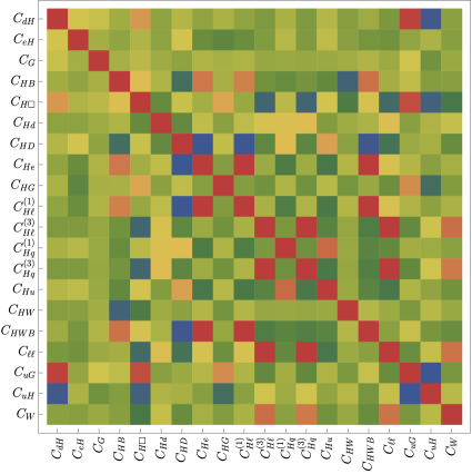
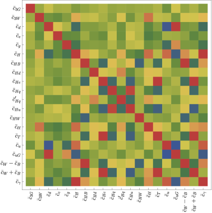
The relative importances of these data sets are also important for the correlations between the constraints on the coefficients of the different operators. These correlations depend on the choice of basis, and we display in Figure 5 the correlation matrices in the Warsaw basis (left) and the SILH basis (right), using the colour code shown in the legend on the right. We see that both bases exhibit high degrees of correlation between some of the coefficients. In particular, in the Warsaw basis the coefficients contributing to EWPTs observables (, , ) as well as the pair (, ) are very correlated, whereas we find strong anti-correlations among operators involved in the LHC measurements (, ), (, ), with operators mostly sensitive to LEP data (, ).
On the other hand, in the SILH basis, we find strong correlations between the operators (, ) due to the impact of diboson measurements, and correlations of the operator with other fermionic operators and , which are mostly constrained by LEP data, see Table 5. As expected, the operator is correlated with the combination of operators , as they both contribute to oblique corrections to the SM couplings 101010 Numerical values of the correlation coefficients are available from https://quark.phy.bnl.gov/ Digital_Data_Archive/SMEFT_GlobalFit/..
| Coefficient | Central value | 1- |
|---|---|---|
| 0.33 | 0.15 | |
| 0.06 | 0.10 | |
| 0.09 | 0.06 | |
| 0.003 | 0.005 | |
| 0.50 | 0.27 | |
| -0.036 | 0.017 | |
| -0.001 | 0.014 | |
| 0.002 | 0.007 | |
| 0.0002 | 0.0003 | |
| 0.002 | 0.003 | |
| -0.015 | 0.011 | |
| -0.002 | 0.003 | |
| -0.017 | 0.013 | |
| 0.000 | 0.011 | |
| -0.002 | 0.014 | |
| 0.006 | 0.007 | |
| -0.009 | 0.006 | |
| 0.7 | 0.4 | |
| -4.8 | 2.6 | |
| -0.05 | 0.06 |
| Coefficient | Central value | 1- |
|---|---|---|
| 0.005 | 0.003 | |
| -0.018 | 0.023 | |
| 0.36 | 0.15 | |
| 0.09 | 0.11 | |
| 0.00002 | 0.00002 | |
| -1.1 | 0.6 | |
| -0.013 | 0.018 | |
| -0.035 | 0.017 | |
| 0.007 | 0.013 | |
| -0.003 | 0.004 | |
| -0.003 | 0.003 | |
| -0.03 | 0.013 | |
| 0.002 | 0.014 | |
| -0.009 | 0.006 | |
| 0.005 | 0.013 | |
| -4.7 | 2.6 | |
| 0.031 | 0.016 | |
| -0.04 | 0.04 | |
| 0.003 | 0.024 | |
| -0.001 | 0.0006 |
| Coefficient | -pole + | at LEP2 | Higgs Run1 | Higgs Run2 | LHC high-pT |
| 36 | 64 | ||||
| 49.6 | 50.4 | ||||
| 2.3 | 97.7 | ||||
| 19 | 81 | ||||
| 19.7 | 80.3 | 0.01 | |||
| 99.88 | 0.04 | 0.07 | |||
| 99.92 | 0.06 | ||||
| 99.99 | 0.01 | ||||
| 34 | 66 | 0.02 | |||
| 99.97 | 0.03 | ||||
| 99.56 | 0.41 | 0.01 | |||
| 99.98 | 0.01 | 0.01 | |||
| 98.6 | 0.96 | 0.19 | 0.23 | 0.07 | |
| 99.5 | 0.2 | 0.3 | 0.04 | ||
| 18 | 82 | ||||
| 57.9 | 0.02 | 8.2 | 33.9 | ||
| 99.66 | 0.32 | 0.01 | 0.01 | ||
| 7.8 | 92.2 | ||||
| 9.5 | 90.5 | ||||
| 96.2 | 3.8 |

6 Implications for Extensions of the Standard Model
6.1 Single-Parameter Models
Ref. [53] gave a complete dictionary in the Warsaw basis [9] for new scalar bosons, vector-like fermions, and vector bosons that contribute to the dimension-six SMEFT operator coefficients at the tree level. We use the notation of Ref. [53] in what follows, unless explicitly stated otherwise. The models that are constrained by our fit are listed in Table 6111111We do not consider model , although it would be constrained by our fit, because its only interaction with the SM is through kinetic mixing with the Higgs field.. All of the vector-like fermion models are constrained by this dataset, whereas it constrains only the color-singlet boson models. It is worth noting that many of these models generate operators that are not constrained by this dataset.
| Name | Spin | Name | Spin | ||||||
|---|---|---|---|---|---|---|---|---|---|
| 0 | 1 | 1 | 0 | 1 | 2 | ||||
| 0 | 1 | 1 | 1 | 1 | 2 | ||||
| 0 | 1 | 2 | 1 | 3 | 0 | ||||
| 0 | 1 | 3 | 0 | 1 | 3 | -1 | |||
| 0 | 1 | 3 | 1 | 3 | 1 | ||||
| 1 | 1 | 1 | 0 | 3 | 1 | ||||
| 1 | 1 | 1 | 1 | 3 | 2 | ||||
| 1 | 1 | 3 | 0 | 3 | 2 | ||||
| 1 | 1 | 3 | 1 | 3 | 2 | ||||
| 1 | 1 | 0 | 3 | 3 | |||||
| 1 | 1 | -1 | 3 | 3 |
We first consider renormalizable versions of the UV-complete models, with bounds on single-parameter models being given in Table 7. The total and the per degree of freedom () in the SM are given in the top row. The subsequent rows show the total and the The first set of models below the SM improve both the and the . For these models we give the 1- preferred range for the modulus of the coupling squared, assuming a mass of 1 TeV, and for the mass assuming a coupling of unity. The middle set of models improve only the . However, we note that in none of these cases is the improvement in either the or the significant. The bottom set of models improve neither the nor the . For each of these models we give instead the 1- upper limit on the modulus of the coupling squared, and the 1- lower limit on the mass. The bound on, or preferred range for, the mass of a particle is a better indicator than the pull of the model of how likely it is to be discovered at the LHC or some other future collider.
The model named in Ref. [53] is equivalent to the Two-Higgs Doublet Model (2HDM); see, e.g., [128] for the corresponding 2HDM notation. We give bounds on the Type-I 2HDM in Table 7, which is characterized in part by having a universal modification of the SM Yukawa couplings. Our fit is only sensitive to the product of couplings in the Type-I 2HDM where
| (13) |
For this reason we consider it a single-parameter model, and we do not perform a comprehensive analysis of the 2HDM. Furthermore, many such analyses already exist, both within [18, 129, 130] and outside [131, 132, 119] the EFT framework. Lastly, note the preferred mass range for in Table 7 assumes the product .
| Model | Coupling | Mass / TeV | ||
| SM | 157 | 0.987 | - | - |
| 156 | 0.986 | |||
| , Type I | 156 | 0.986 | ||
| 155 | 0.984 | |||
| 155 | 0.978 | |||
| 155 | 0.984 | |||
| 157 | 0.993 | |||
| 156 | 0.990 | |||
| 157 | 0.992 | |||
| 156 | 0.990 | |||
| 157 | 0.992 | |||
| 157 | 0.993 | |||
| 157 | 0.993 | |||
| 157 | 0.993 | |||
| 157 | 0.993 | |||
| 157 | 0.993 | |||
| 157 | 0.993 | |||
| 157 | 0.993 | |||
| 157 | 0.993 |
6.2 Multi-Parameter Models
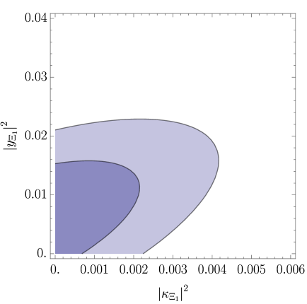
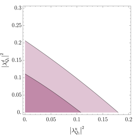
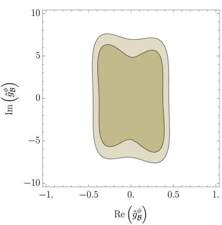
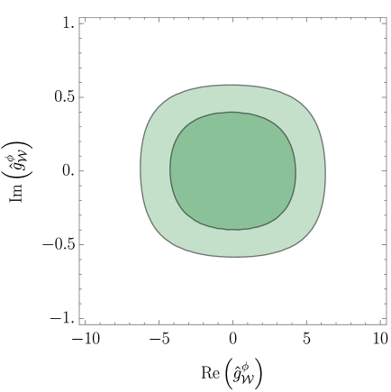
We have also investigated a number of two-parameter scenarios, namely the models , , , and defined in Table 6. For the latter two models we have assumed that all four-fermion operator coefficients are zero, both to reduce the parameter space and to avoid the bounds from dijet and dilepton searches at the LHC, which are not included in our fit. The viable parameter space is each of these models assuming a mass of 1 TeV is shown in Figure 6. As previously, the regions shaded in darker and lighter colours are allowed at 1 and 2 , respectively.
6.3 Non-Renormalizable Models
We now relax the assumption of renormalizability in the UV models. In particular, dimension-5 operators are added to the UV models. A combination of super-renormalizable and non-renormalizable operators in a UV theory can generate higher-dimensional operators with arbitrary coefficients in the corresponding low energy EFT [53, 133]. In a UV completion of this intermediate EFT, should it exist, these dimension-5 operators can only be generated at loop level [53, 134]. However if this UV-completion is strongly-interacting, the coefficients generated may be sizeable, see Ref. [135] for an explicit example.
The results of fits to the non-renormalizable versions of the models in Table 6 are presented in terms of the eigensystem of the covariance matrix for the least-squares estimators in Eqs. (14), (15), (16), (17), (18), (19), (20), (21), (22), (23), (24), (25), (26), (27), and (28) below. The chi-squared and goodness-of-fit are given, as are any relations between the coefficients generated when they exist. Note that only contributions to the eigenvectors at the percent level or larger are presented.
-
•
: , .
(14) -
•
: , , .
(15) -
•
: , , .
(16) -
•
: , .
(17) -
•
: , , .
(18) -
•
: , .
(19) -
•
: , , .
(20) -
•
: , , .
(21) -
•
: , , .
(22) -
•
: , , .
(23) -
•
: , .
(24) -
•
: , .
(25) -
•
: , ,
(26) -
•
: , , .
(27) -
•
: , , .
(28)
6.4 Stop Squarks in the MSSM
Finally, as an example how the constraints on the SMEFT coefficients can be used to constrain possible BSM physics at the loop level, we consider the minimal supersymmetric extension of the SM (the MSSM). Among the sparticles for which the data may be most constraining are the stops, by virtue of their large couplings to the Higgs field. Moreover, SMEFT constraints are of particular interest for stops also because the constraints from direct searches are model-dependent and often require the understanding of complicated final states to which the LHC has reduced sensitivity, whereas the SMEFT constraints are relatively model-independent. Run 1 LHC data were used to constrain degenerate stops in [54, 55], and non-degenerate stops in [56], where comparisons were made between the constraints obtained using the SMEFT and an exact one-loop calculation. It was found there that the SMEFT and exact one-loop results were quite similar, except in regions of parameter space where the data were insensitive even to very light stops.
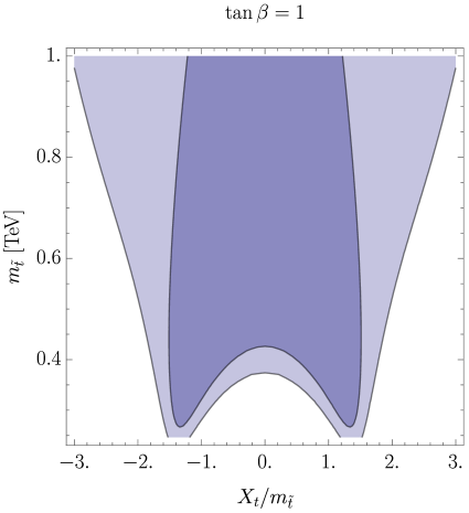
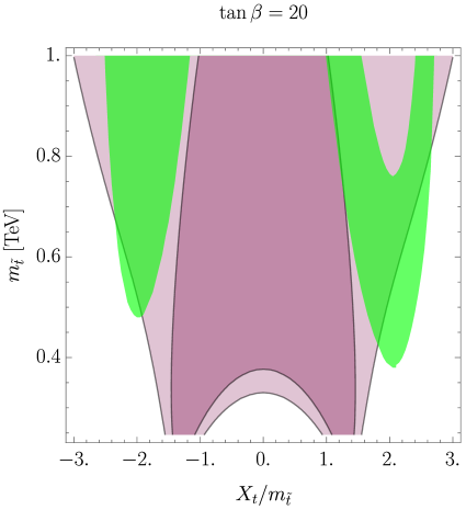
Here we make a new comparison of the degenerate stop case using Run 2 LHC data. Figure 7 shows the SMEFT constraints in the plane of the degenerate stop mass and the stop mixing parameter for the two choices and 20 of the ratio of Higgs vev’s, where the darker and lighter blue regions correspond to 1- and 2- ranges, respectively. We note that the kinematic ranges of the LHC Run 2 Higgs data used in our analysis extend typically to GeV (see Table 3). The LHC data that we use include a tail that may extend to higher , but this has less weight in the global fit, see the last column in Table 5. We therefore expect the SMEFT analysis to be reasonably reliable for GeV.
By way of comparison, although the LHC limits on the stop mass may extend as far as TeV under certain assumptions on the sparticle spectrum [136, 137], they are sensitive to the value assumed for the lightest supersymmetric particle , disappearing entirely for GeV and having holes for some values of GeV when GeV. We conclude that the indirect SMEFT constraint is highly competitive, despite the fact that the Wilson coefficients are generated only at the loop level.
7 Conclusions
We have presented in this paper a first combined global analysis within the SMEFT of the available precision electroweak data, diboson production data from LEP and the LHC, and the data on Higgs production from Runs 1 and 2 of the LHC. Our analysis takes into account all the 20 dimension-6 operators that are relevant to these processes. We emphasize that these data should be analyzed jointly, as the constraints from different data categories are synergistic, complementary and of comparable importance. This point is exemplified in Fig. 1, where we see explicitly the complementarity of the constraints from -pole, mass, and LEP 2 production measurements (orange) and LHC Higgs production measurements (green) on the oblique parameters and , which are proportional to the dimension-6 operator coefficients and , respectively.
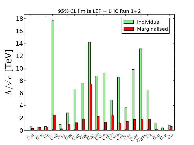
The sensitivities to the scales of the operators in the Warsaw basis for an Wilson coefficient is summarised in Fig. 8. Overviews of our results are shown in Figs. 2 (Warsaw basis) and 3 (SILH basis), where we see in the upper panels the results of fits where all the 20 operator coefficients are allowed to vary simultaneously, and in the lower panels results where the operators are switched on one at a time. Fig. 2 also shows comparisons with fits omitting the LHC Run 2 data, and Fig. 4 displays explicitly the reductions in the uncertainties in the operator coefficients in the Warsaw basis when the LHC Run 2 data are included. Fig. 3 (SILH basis) shows a comparison with a fit to the precision -pole and -mass data alone, and a comparison with the results of [18], which included Higgs results from Run 1 of the LHC only. Numerical results from the fits in the Warsaw and SILH bases are tabulated in Table 4, and impacts of the different datasets on the global fit in the Warsaw basis are shown numerically in Table 5. Whereas the constraints from the precision electroweak observables have evolved slowly, those from Higgs production are now much stronger than from Run 1, due to the availability of much kinematical information as well as the increased statistics. Correlations between the operator coefficients in the two operator bases are shown in Fig. 5.
Table 8 compares the qualities of the fits within the SM and the SMEFT, displaying their respective , , and -values. The top line is for a fit to the SM and the middle line is for a fit to the SMEFT allowing all 20 coefficients to vary, whilst the bottom line assumes a UV-completion of the SMEFT (indicated with with a ) that is renormalizable and weakly-coupled. These assumptions allow 13 coefficients to be non-zero, and in the Warsaw basis the coefficients set to zero in this case are , , , , , , and . We see that neither the full SMEFT nor the SMEFT⋆ give fits that are significant improvements on the SM fit, which has already a very acceptable -value. Thus, these fits provide no sign or evidence of any physics beyond the Standard Model.
| Theory | -value | ||
|---|---|---|---|
| SM | 157 | 0.987 | 0.532 |
| SMEFT | 137 | 0.987 | 0.528 |
| SMEFT⋆ | 143 | 0.977 | 0.564 |
Our new constraints on the dimension-6 operator coefficients can be applied to variety of specific BSM scenarios. Specifically, we have studied extensions of the SM that can make tree-level contributions to the operator coefficients, as tabulated in Table 6, using the dictionary proposed in [53]: see Fig. 6 and the numerical results in Section 6. We have also explored the constraints imposed by the global fit on stops in the MSSM, which contribute to the operator coefficients only at the loop level, see Fig. 7. These constraints are model-independent, and competitive with the model-dependent constraints on stops from Run 2 of the LHC.
We can expect in the near future further substantial increases in the amounts of information from diboson and Higgs production at the LHC as the ATLAS and CMS Collaborations complete their analyses of data from Run 2. We emphasize the importance to SMEFT analyses of making available as much information as possible on the kinematics of diboson and Higgs production, since the and invariant mass distributions, in particular, are more sensitive to dimension-6 operator coefficients than are the integrated production rates. In this way maximal information can be extracted from the data and used, via a SMEFT analysis, to constrain possible BSM scenarios, as we have illustrated in this paper. We cannot know whether such an analysis will reveal any BSM physics, but in this way we will give the search for new physics our best shot.
Acknowledgements
We thank Ilaria Brivio, Pier Paolo Giardino, Martín González-Alonso and Michael Trott for useful discussions, and Jérémie Quevillon for the MSSM Higgs mass calculations. The work of JE was supported partly by the United Kingdom STFC Grant ST/P000258/1 and partly by the Estonian Research Council via a Mobilitas Pluss grant. VS acknowledges support from the Science and Technology Facilities Council (ST/P000819/1). The work of CWM was supported by the United States Department of Energy under Grant Contract DE-SC0012704. The work of TY was supported by a Junior Research Fellowship from Gonville and Caius College and partially supported by STFC consolidated grant ST/P000681/1.
Supplementary Material
The complete function in both the SILH and Warsaw bases as well as all of our predictions made using are available online at https://quark.phy.bnl.gov/Digital_Data_Archive/SMEFT_GlobalFit/.
References
- [1] LHC Higgs Cross Section Working Group Collaboration, D. de Florian et al., “Handbook of LHC Higgs Cross Sections: 4. Deciphering the Nature of the Higgs Sector,” arXiv:1610.07922 [hep-ph].
- [2] I. Brivio and M. Trott, “The Standard Model as an Effective Field Theory,” arXiv:1706.08945 [hep-ph].
- [3] A. Falkowski, “Effective field theory approach to LHC Higgs data,” Pramana 87 no. 3, (2016) 39, arXiv:1505.00046 [hep-ph].
- [4] S. Willenbrock and C. Zhang, “Effective Field Theory Beyond the Standard Model,” Ann. Rev. Nucl. Part. Sci. 64 (2014) 83–100, arXiv:1401.0470 [hep-ph].
- [5] S. Weinberg, “Baryon and Lepton Nonconserving Processes,” Phys. Rev. Lett. 43 (1979) 1566–1570.
- [6] W. Buchmuller and D. Wyler, “Effective Lagrangian Analysis of New Interactions and Flavor Conservation,” Nucl. Phys. B268 (1986) 621–653.
- [7] L. Lehman, “Extending the Standard Model Effective Field Theory with the Complete Set of Dimension-7 Operators,” Phys. Rev. D90 no. 12, (2014) 125023, arXiv:1410.4193 [hep-ph].
- [8] B. Henning, X. Lu, T. Melia, and H. Murayama, “2, 84, 30, 993, 560, 15456, 11962, 261485, …: Higher dimension operators in the SM EFT,” JHEP 08 (2017) 016, arXiv:1512.03433 [hep-ph].
- [9] B. Grzadkowski, M. Iskrzynski, M. Misiak, and J. Rosiek, “Dimension-Six Terms in the Standard Model Lagrangian,” JHEP 10 (2010) 085, arXiv:1008.4884 [hep-ph].
- [10] R. Contino, M. Ghezzi, C. Grojean, M. Muhlleitner, and M. Spira, “Effective Lagrangian for a light Higgs-like scalar,” JHEP 07 (2013) 035, arXiv:1303.3876 [hep-ph].
- [11] R. S. Gupta, A. Pomarol, and F. Riva, “BSM Primary Effects,” Phys. Rev. D91 no. 3, (2015) 035001, arXiv:1405.0181 [hep-ph].
- [12] E. Massó, “An Effective Guide to Beyond the Standard Model Physics,” JHEP 10 (2014) 128, arXiv:1406.6376 [hep-ph].
- [13] A. Falkowski, B. Fuks, K. Mawatari, K. Mimasu, F. Riva, and V. Sanz, “Rosetta: an operator basis translator for Standard Model effective field theory,” Eur. Phys. J. C75 no. 12, (2015) 583, arXiv:1508.05895 [hep-ph].
- [14] J. Aebischer et al., “WCxf: an exchange format for Wilson coefficients beyond the Standard Model,” arXiv:1712.05298 [hep-ph].
- [15] Z. Han and W. Skiba, “Effective theory analysis of precision electroweak data,” Phys. Rev. D71 (2005) 075009, arXiv:hep-ph/0412166 [hep-ph].
- [16] A. Pomarol and F. Riva, “Towards the Ultimate SM Fit to Close in on Higgs Physics,” JHEP 01 (2014) 151, arXiv:1308.2803 [hep-ph].
- [17] J. Ellis, V. Sanz, and T. You, “Complete Higgs Sector Constraints on Dimension-6 Operators,” JHEP 07 (2014) 036, arXiv:1404.3667 [hep-ph].
- [18] J. Ellis, V. Sanz, and T. You, “The Effective Standard Model after LHC Run I,” JHEP 03 (2015) 157, arXiv:1410.7703 [hep-ph].
- [19] C. W. Murphy, “Statistical approach to Higgs boson couplings in the standard model effective field theory,” Phys. Rev. D97 no. 1, (2018) 015007, arXiv:1710.02008 [hep-ph].
- [20] A. Falkowski and F. Riva, “Model-independent precision constraints on dimension-6 operators,” JHEP 02 (2015) 039, arXiv:1411.0669 [hep-ph].
- [21] A. Efrati, A. Falkowski, and Y. Soreq, “Electroweak constraints on flavorful effective theories,” JHEP 07 (2015) 018, arXiv:1503.07872 [hep-ph].
- [22] A. Falkowski, M. Gonzalez-Alonso, A. Greljo, and D. Marzocca, “Global constraints on anomalous triple gauge couplings in effective field theory approach,” Phys. Rev. Lett. 116 no. 1, (2016) 011801, arXiv:1508.00581 [hep-ph].
- [23] A. Falkowski and K. Mimouni, “Model independent constraints on four-lepton operators,” JHEP 02 (2016) 086, arXiv:1511.07434 [hep-ph].
- [24] A. Falkowski, M. Gonzalez-Alonso, A. Greljo, D. Marzocca, and M. Son, “Anomalous Triple Gauge Couplings in the Effective Field Theory Approach at the LHC,” JHEP 02 (2017) 115, arXiv:1609.06312 [hep-ph].
- [25] A. Falkowski, M. González-Alonso, and K. Mimouni, “Compilation of low-energy constraints on 4-fermion operators in the SMEFT,” JHEP 08 (2017) 123, arXiv:1706.03783 [hep-ph].
- [26] A. Falkowski, G. Grilli di Cortona, and Z. Tabrizi, “Future DUNE constraints on EFT,” arXiv:1802.08296 [hep-ph].
- [27] T. Corbett, O. J. P. Eboli, J. Gonzalez-Fraile, and M. C. Gonzalez-Garcia, “Robust Determination of the Higgs Couplings: Power to the Data,” Phys. Rev. D87 (2013) 015022, arXiv:1211.4580 [hep-ph].
- [28] T. Corbett, O. J. P. Éboli, J. Gonzalez-Fraile, and M. C. Gonzalez-Garcia, “Determining Triple Gauge Boson Couplings from Higgs Data,” Phys. Rev. Lett. 111 (2013) 011801, arXiv:1304.1151 [hep-ph].
- [29] C. Englert, R. Kogler, H. Schulz, and M. Spannowsky, “Higgs coupling measurements at the LHC,” Eur. Phys. J. C76 no. 7, (2016) 393, arXiv:1511.05170 [hep-ph].
- [30] A. Buckley, C. Englert, J. Ferrando, D. J. Miller, L. Moore, K. Nördstrom, M. Russell, and C. D. White, “Results from TopFitter,” PoS CKM2016 (2016) 127, arXiv:1612.02294 [hep-ph].
- [31] A. Buckley, C. Englert, J. Ferrando, D. J. Miller, L. Moore, M. Russell, and C. D. White, “Constraining top quark effective theory in the LHC Run II era,” JHEP 04 (2016) 015, arXiv:1512.03360 [hep-ph].
- [32] T. Corbett, O. J. P. Eboli, D. Goncalves, J. Gonzalez-Fraile, T. Plehn, and M. Rauch, “The Higgs Legacy of the LHC Run I,” JHEP 08 (2015) 156, arXiv:1505.05516 [hep-ph].
- [33] A. Butter, O. J. P. Éboli, J. Gonzalez-Fraile, M. C. Gonzalez-Garcia, T. Plehn, and M. Rauch, “The Gauge-Higgs Legacy of the LHC Run I,” JHEP 07 (2016) 152, arXiv:1604.03105 [hep-ph].
- [34] B. Dumont, S. Fichet, and G. von Gersdorff, “A Bayesian view of the Higgs sector with higher dimensional operators,” JHEP 07 (2013) 065, arXiv:1304.3369 [hep-ph].
- [35] J. de Blas, M. Ciuchini, E. Franco, S. Mishima, M. Pierini, L. Reina, and L. Silvestrini, “The Global Electroweak and Higgs Fits in the LHC era,” in 5th Large Hadron Collider Physics Conference (LHCP 2017) Shanghai, China, May 15-20, 2017. 2017. arXiv:1710.05402 [hep-ph].
- [36] J. de Blas, M. Ciuchini, E. Franco, S. Mishima, M. Pierini, L. Reina, and L. Silvestrini, “Electroweak precision constraints at present and future colliders,” PoS ICHEP2016 (2017) 690, arXiv:1611.05354 [hep-ph].
- [37] L. Berthier and M. Trott, “Towards consistent Electroweak Precision Data constraints in the SMEFT,” JHEP 05 (2015) 024, arXiv:1502.02570 [hep-ph].
- [38] L. Berthier and M. Trott, “Consistent constraints on the Standard Model Effective Field Theory,” JHEP 02 (2016) 069, arXiv:1508.05060 [hep-ph].
- [39] L. Berthier, M. Bjorn, and M. Trott, “Incorporating doubly resonant data in a global fit of SMEFT parameters to lift flat directions,” JHEP 09 (2016) 157, arXiv:1606.06693 [hep-ph].
- [40] I. Brivio and M. Trott, “Scheming in the SMEFT… and a reparameterization invariance!,” JHEP 07 (2017) 148, arXiv:1701.06424 [hep-ph].
- [41] SLD Electroweak Group, DELPHI, ALEPH, SLD, SLD Heavy Flavour Group, OPAL, LEP Electroweak Working Group, L3 Collaboration, S. Schael et al., “Precision electroweak measurements on the resonance,” Phys. Rept. 427 (2006) 257–454, arXiv:hep-ex/0509008 [hep-ex].
- [42] CDF, D0 Collaboration, T. A. Aaltonen et al., “Combination of CDF and D0 -Boson Mass Measurements,” Phys. Rev. D88 no. 5, (2013) 052018, arXiv:1307.7627 [hep-ex].
- [43] ALEPH Collaboration, A. Heister et al., “Measurement of W-pair production in e+ e- collisions at centre-of-mass energies from 183-GeV to 209-GeV,” Eur. Phys. J. C38 (2004) 147–160.
- [44] L3 Collaboration, P. Achard et al., “Measurement of the cross section of W-boson pair production at LEP,” Phys. Lett. B600 (2004) 22–40, arXiv:hep-ex/0409016 [hep-ex].
- [45] OPAL Collaboration, G. Abbiendi et al., “Measurement of the e+ e- W+ W- cross section and W decay branching fractions at LEP,” Eur. Phys. J. C52 (2007) 767–785, arXiv:0708.1311 [hep-ex].
- [46] DELPHI, OPAL, LEP Electroweak, ALEPH, L3 Collaboration, S. Schael et al., “Electroweak Measurements in Electron-Positron Collisions at W-Boson-Pair Energies at LEP,” Phys. Rept. 532 (2013) 119–244, arXiv:1302.3415 [hep-ex].
- [47] ATLAS Collaboration, M. Aaboud et al., “Measurement of the production cross section in collisions at a centre-of-mass energy of = 13 TeV with the ATLAS experiment,” Phys. Lett. B773 (2017) 354–374, arXiv:1702.04519 [hep-ex].
- [48] T. Dorigo, “Hadron Collider Searches for Diboson Resonances,” arXiv:1802.00354 [hep-ex].
- [49] ATLAS, CMS Collaboration, G. Aad et al., “Measurements of the Higgs boson production and decay rates and constraints on its couplings from a combined ATLAS and CMS analysis of the LHC pp collision data at and 8 TeV,” JHEP 08 (2016) 045, arXiv:1606.02266 [hep-ex].
- [50] Z. Zhang, “Time to Go Beyond Triple-Gauge-Boson-Coupling Interpretation of Pair Production,” Phys. Rev. Lett. 118 no. 1, (2017) 011803, arXiv:1610.01618 [hep-ph].
- [51] J. Baglio, S. Dawson, and I. M. Lewis, “An NLO QCD effective field theory analysis of production at the LHC including fermionic operators,” Phys. Rev. D96 no. 7, (2017) 073003, arXiv:1708.03332 [hep-ph].
- [52] G. F. Giudice, C. Grojean, A. Pomarol, and R. Rattazzi, “The Strongly-Interacting Light Higgs,” JHEP 06 (2007) 045, arXiv:hep-ph/0703164 [hep-ph].
- [53] J. de Blas, J. C. Criado, M. Perez-Victoria, and J. Santiago, “Effective description of general extensions of the Standard Model: the complete tree-level dictionary,” arXiv:1711.10391 [hep-ph].
- [54] B. Henning, X. Lu, and H. Murayama, “How to use the Standard Model effective field theory,” JHEP 01 (2016) 023, arXiv:1412.1837 [hep-ph].
- [55] B. Henning, X. Lu, and H. Murayama, “What do precision Higgs measurements buy us?,” arXiv:1404.1058 [hep-ph].
- [56] A. Drozd, J. Ellis, J. Quevillon, and T. You, “Comparing EFT and Exact One-Loop Analyses of Non-Degenerate Stops,” JHEP 06 (2015) 028, arXiv:1504.02409 [hep-ph].
- [57] A. Drozd, J. Ellis, J. Quevillon, and T. You, “The Universal One-Loop Effective Action,” JHEP 03 (2016) 180, arXiv:1512.03003 [hep-ph].
- [58] F. del Aguila, Z. Kunszt, and J. Santiago, “One-loop effective lagrangians after matching,” Eur. Phys. J. C76 no. 5, (2016) 244, arXiv:1602.00126 [hep-ph].
- [59] M. Boggia, R. Gomez-Ambrosio, and G. Passarino, “Low energy behaviour of standard model extensions,” JHEP 05 (2016) 162, arXiv:1603.03660 [hep-ph].
- [60] B. Henning, X. Lu, and H. Murayama, “One-loop Matching and Running with Covariant Derivative Expansion,” JHEP 01 (2018) 123, arXiv:1604.01019 [hep-ph].
- [61] S. A. R. Ellis, J. Quevillon, T. You, and Z. Zhang, “Mixed heavy-light matching in the Universal One-Loop Effective Action,” Phys. Lett. B762 (2016) 166–176, arXiv:1604.02445 [hep-ph].
- [62] J. Fuentes-Martin, J. Portoles, and P. Ruiz-Femenia, “Integrating out heavy particles with functional methods: a simplified framework,” JHEP 09 (2016) 156, arXiv:1607.02142 [hep-ph].
- [63] Z. Zhang, “Covariant diagrams for one-loop matching,” JHEP 05 (2017) 152, arXiv:1610.00710 [hep-ph].
- [64] S. A. R. Ellis, J. Quevillon, T. You, and Z. Zhang, “Extending the Universal One-Loop Effective Action: Heavy-Light Coefficients,” JHEP 08 (2017) 054, arXiv:1706.07765 [hep-ph].
- [65] R. Contino, A. Falkowski, F. Goertz, C. Grojean, and F. Riva, “On the Validity of the Effective Field Theory Approach to SM Precision Tests,” JHEP 07 (2016) 144, arXiv:1604.06444 [hep-ph].
- [66] C. Grojean, E. E. Jenkins, A. V. Manohar, and M. Trott, “Renormalization Group Scaling of Higgs Operators and ,” JHEP 04 (2013) 016, arXiv:1301.2588 [hep-ph].
- [67] J. Elias-Miro, J. R. Espinosa, E. Massó, and A. Pomarol, “Renormalization of dimension-six operators relevant for the Higgs decays ,” JHEP 08 (2013) 033, arXiv:1302.5661 [hep-ph].
- [68] J. Elias-Miro, J. R. Espinosa, E. Massó, and A. Pomarol, “Higgs windows to new physics through d=6 operators: constraints and one-loop anomalous dimensions,” JHEP 11 (2013) 066, arXiv:1308.1879 [hep-ph].
- [69] E. E. Jenkins, A. V. Manohar, and M. Trott, “Renormalization Group Evolution of the Standard Model Dimension Six Operators I: Formalism and lambda Dependence,” JHEP 10 (2013) 087, arXiv:1308.2627 [hep-ph].
- [70] E. E. Jenkins, A. V. Manohar, and M. Trott, “Renormalization Group Evolution of the Standard Model Dimension Six Operators II: Yukawa Dependence,” JHEP 01 (2014) 035, arXiv:1310.4838 [hep-ph].
- [71] R. Alonso, E. E. Jenkins, A. V. Manohar, and M. Trott, “Renormalization Group Evolution of the Standard Model Dimension Six Operators III: Gauge Coupling Dependence and Phenomenology,” JHEP 04 (2014) 159, arXiv:1312.2014 [hep-ph].
- [72] R. Alonso, H.-M. Chang, E. E. Jenkins, A. V. Manohar, and B. Shotwell, “Renormalization group evolution of dimension-six baryon number violating operators,” Phys. Lett. B734 (2014) 302–307, arXiv:1405.0486 [hep-ph].
- [73] E. E. Jenkins, A. V. Manohar, and P. Stoffer, “Low-Energy Effective Field Theory below the Electroweak Scale: Operators and Matching,” arXiv:1709.04486 [hep-ph].
- [74] A. Celis, J. Fuentes-Martin, A. Vicente, and J. Virto, “DsixTools: The Standard Model Effective Field Theory Toolkit,” Eur. Phys. J. C77 no. 6, (2017) 405, arXiv:1704.04504 [hep-ph].
- [75] J. Aebischer, A. Crivellin, M. Fael, and C. Greub, “Matching of gauge invariant dimension-six operators for and transitions,” JHEP 05 (2016) 037, arXiv:1512.02830 [hep-ph].
- [76] J. Aebischer, M. Fael, C. Greub, and J. Virto, “B physics Beyond the Standard Model at One Loop: Complete Renormalization Group Evolution below the Electroweak Scale,” JHEP 09 (2017) 158, arXiv:1704.06639 [hep-ph].
- [77] E. E. Jenkins, A. V. Manohar, and P. Stoffer, “Low-Energy Effective Field Theory below the Electroweak Scale: Anomalous Dimensions,” JHEP 01 (2018) 084, arXiv:1711.05270 [hep-ph].
- [78] M. Trott, “EWPD in the SMEFT and the one loop decay width,” in Proceedings, 52nd Rencontres de Moriond on Electroweak Interactions and Unified Theories: La Thuile, Italy, March 18-25, 2017. 2017. arXiv:1705.05652 [hep-ph].
- [79] C. Hartmann, W. Shepherd, and M. Trott, “The decay width in the SMEFT: and corrections at one loop,” JHEP 03 (2017) 060, arXiv:1611.09879 [hep-ph].
- [80] G. Passarino and M. Trott, “The Standard Model Effective Field Theory and Next to Leading Order,” arXiv:1610.08356 [hep-ph].
- [81] C. Hartmann and M. Trott, “Higgs Decay to Two Photons at One Loop in the Standard Model Effective Field Theory,” Phys. Rev. Lett. 115 no. 19, (2015) 191801, arXiv:1507.03568 [hep-ph].
- [82] R. Gauld, B. D. Pecjak, and D. J. Scott, “QCD radiative corrections for in the Standard Model Dimension-6 EFT,” Phys. Rev. D94 no. 7, (2016) 074045, arXiv:1607.06354 [hep-ph].
- [83] S. Dawson and P. P. Giardino, “Higgs Decays to and in the SMEFT: an NLO analysis,” arXiv:1801.01136 [hep-ph].
- [84] L. Lehman and A. Martin, “Hilbert Series for Constructing Lagrangians: expanding the phenomenologist’s toolbox,” Phys. Rev. D91 (2015) 105014, arXiv:1503.07537 [hep-ph].
- [85] L. Lehman and A. Martin, “Low-derivative operators of the Standard Model effective field theory via Hilbert series methods,” JHEP 02 (2016) 081, arXiv:1510.00372 [hep-ph].
- [86] B. Henning, X. Lu, T. Melia, and H. Murayama, “Hilbert series and operator bases with derivatives in effective field theories,” Commun. Math. Phys. 347 no. 2, (2016) 363–388, arXiv:1507.07240 [hep-th].
- [87] B. Henning, X. Lu, T. Melia, and H. Murayama, “Operator bases, -matrices, and their partition functions,” JHEP 10 (2017) 199, arXiv:1706.08520 [hep-th].
- [88] J. Brehmer, F. Kling, T. Plehn, and T. M. P. Tait, “Better Higgs-CP Tests Through Information Geometry,” arXiv:1712.02350 [hep-ph].
- [89] J. H. Kim, Y. Sakaki, and M. Son, “Combined analysis of double Higgs production via gluon fusion at the HL-LHC in the effective field theory approach,” arXiv:1801.06093 [hep-ph].
- [90] A. Azatov, R. Contino, G. Panico, and M. Son, “Effective field theory analysis of double Higgs boson production via gluon fusion,” Phys. Rev. D92 no. 3, (2015) 035001, arXiv:1502.00539 [hep-ph].
- [91] J. Baglio, A. Djouadi, R. Gröber, M. M. Mühlleitner, J. Quevillon, and M. Spira, “The measurement of the Higgs self-coupling at the LHC: theoretical status,” JHEP 04 (2013) 151, arXiv:1212.5581 [hep-ph].
- [92] S. Di Vita, C. Grojean, G. Panico, M. Riembau, and T. Vantalon, “A global view on the Higgs self-coupling,” JHEP 09 (2017) 069, arXiv:1704.01953 [hep-ph].
- [93] A. Alves, T. Ghosh, and K. Sinha, “Can We Discover Double Higgs Production at the LHC?,” Phys. Rev. D96 no. 3, (2017) 035022, arXiv:1704.07395 [hep-ph].
- [94] S. Dawson and C. W. Murphy, “Standard Model EFT and Extended Scalar Sectors,” Phys. Rev. D96 no. 1, (2017) 015041, arXiv:1704.07851 [hep-ph].
- [95] S. Di Vita, G. Durieux, C. Grojean, J. Gu, Z. Liu, G. Panico, M. Riembau, and T. Vantalon, “A global view on the Higgs self-coupling at lepton colliders,” JHEP 02 (2018) 178, arXiv:1711.03978 [hep-ph].
- [96] D. Barducci et al., “Interpreting top-quark LHC measurements in the standard-model effective field theory,” arXiv:1802.07237 [hep-ph].
- [97] F. Krauss, S. Kuttimalai, and T. Plehn, “LHC multijet events as a probe for anomalous dimension-six gluon interactions,” Phys. Rev. D95 no. 3, (2017) 035024, arXiv:1611.00767 [hep-ph].
- [98] A. Alloul, B. Fuks, and V. Sanz, “Phenomenology of the Higgs Effective Lagrangian via FEYNRULES,” JHEP 04 (2014) 110, arXiv:1310.5150 [hep-ph].
- [99] I. Brivio, Y. Jiang, and M. Trott, “The SMEFTsim package, theory and tools,” JHEP 12 (2017) 070, arXiv:1709.06492 [hep-ph].
- [100] ATLAS Collaboration, M. Aaboud et al., “Measurement of the -boson mass in pp collisions at TeV with the ATLAS detector,” Eur. Phys. J. C78 no. 2, (2018) 110, arXiv:1701.07240 [hep-ex].
- [101] ATLAS Collaboration, G. Aad et al., “Measurements of the Higgs boson production and decay rates and coupling strengths using pp collision data at and 8 TeV in the ATLAS experiment,” Eur. Phys. J. C76 no. 1, (2016) 6, arXiv:1507.04548 [hep-ex].
- [102] CMS Collaboration, A. M. Sirunyan et al., “Inclusive search for a highly boosted Higgs boson decaying to a bottom quark-antiquark pair,” Phys. Rev. Lett. 120 no. 7, (2018) 071802, arXiv:1709.05543 [hep-ex].
- [103] CMS Collaboration, A. M. Sirunyan et al., “Evidence for the Higgs boson decay to a bottom quark?antiquark pair,” Phys. Lett. B780 (2018) 501–532, arXiv:1709.07497 [hep-ex].
- [104] CMS Collaboration, A. M. Sirunyan et al., “Search for H production in the decay channel with leptonic decays in proton-proton collisions at 13 TeV,” arXiv:1804.03682 [hep-ex].
- [105] CMS Collaboration, A. M. Sirunyan et al., “Evidence for associated production of a Higgs boson with a top quark pair in final states with electrons, muons, and hadronically decaying leptons at 13 TeV,” arXiv:1803.05485 [hep-ex].
- [106] CMS Collaboration Collaboration, “Measurements of properties of the Higgs boson decaying to a W boson pair in pp collisions at ,” Tech. Rep. CMS-PAS-HIG-16-042, CERN, Geneva, 2018. http://cds.cern.ch/record/2308255.
- [107] CMS Collaboration, A. M. Sirunyan et al., “Measurements of Higgs boson properties in the diphoton decay channel in proton-proton collisions at 13 TeV,” arXiv:1804.02716 [hep-ex].
- [108] CMS Collaboration, A. M. Sirunyan et al., “Measurements of properties of the Higgs boson decaying into the four-lepton final state in pp collisions at TeV,” JHEP 11 (2017) 047, arXiv:1706.09936 [hep-ex].
- [109] CMS Collaboration, A. M. Sirunyan et al., “Observation of the Higgs boson decay to a pair of leptons with the CMS detector,” Phys. Lett. B779 (2018) 283–316, arXiv:1708.00373 [hep-ex].
- [110] ATLAS Collaboration, M. Aaboud et al., “Search for the dimuon decay of the Higgs boson in collisions at = 13 TeV with the ATLAS detector,” Phys. Rev. Lett. 119 no. 5, (2017) 051802, arXiv:1705.04582 [hep-ex].
- [111] ATLAS Collaboration, M. Aaboud et al., “Evidence for the decay with the ATLAS detector,” JHEP 12 (2017) 024, arXiv:1708.03299 [hep-ex].
- [112] ATLAS Collaboration, M. Aaboud et al., “Search for the Standard Model Higgs boson produced in association with top quarks and decaying into a pair in collisions at = 13 TeV with the ATLAS detector,” arXiv:1712.08895 [hep-ex].
- [113] ATLAS Collaboration, M. Aaboud et al., “Evidence for the associated production of the Higgs boson and a top quark pair with the ATLAS detector,” Phys. Rev. D97 no. 7, (2018) 072003, arXiv:1712.08891 [hep-ex].
- [114] ATLAS Collaboration Collaboration, “Measurement of gluon fusion and vector boson fusion Higgs boson production cross-sections in the decay channel in pp collisions at TeV with the ATLAS detector,” Tech. Rep. ATLAS-CONF-2018-004, CERN, Geneva, Mar, 2018. https://cds.cern.ch/record/2308392.
- [115] ATLAS Collaboration Collaboration, “Combined measurements of Higgs boson production and decay in the and channels using 13 TeV pp collision data collected with the ATLAS experiment,” Tech. Rep. ATLAS-CONF-2017-047, CERN, Geneva, Jul, 2017. http://cds.cern.ch/record/2273854.
- [116] ATLAS Collaboration Collaboration, “Measurements of the Higgs boson production cross section via Vector Boson Fusion and associated production in the decay mode with the ATLAS detector at = 13 TeV,” Tech. Rep. ATLAS-CONF-2016-112, CERN, Geneva, Nov, 2016. http://cds.cern.ch/record/2231811.
- [117] C. Hays, V. Sanz Gonzalez, and G. Zemaityte, “Constraining EFT parameters using simplified template cross sections,”. https://cds.cern.ch/record/2290628.
- [118] J. de Blas, O. Eberhardt, and C. Krause, “Current and future constraints on Higgs couplings in the nonlinear Effective Theory,” arXiv:1803.00939 [hep-ph].
- [119] J. Haller, A. Hoecker, R. Kogler, K. Mönig, T. Peiffer, and J. Stelzer, “Update of the global electroweak fit and constraints on two-Higgs-doublet models,” arXiv:1803.01853 [hep-ph].
- [120] Particle Data Group Collaboration, C. Patrignani et al., “Review of Particle Physics,” Chin. Phys. C40 no. 10, (2016) 100001.
- [121] D. C. Kennedy and B. W. Lynn, “Electroweak Radiative Corrections with an Effective Lagrangian: Four Fermion Processes,” Nucl. Phys. B322 (1989) 1–54.
- [122] B. Holdom and J. Terning, “Large corrections to electroweak parameters in technicolor theories,” Phys. Lett. B247 (1990) 88–92.
- [123] M. Golden and L. Randall, “Radiative Corrections to Electroweak Parameters in Technicolor Theories,” Nucl. Phys. B361 (1991) 3–23.
- [124] G. Altarelli and R. Barbieri, “Vacuum polarization effects of new physics on electroweak processes,” Phys. Lett. B253 (1991) 161–167.
- [125] B. Grinstein and M. B. Wise, “Operator analysis for precision electroweak physics,” Phys. Lett. B265 (1991) 326–334.
- [126] M. E. Peskin and T. Takeuchi, “Estimation of oblique electroweak corrections,” Phys. Rev. D46 (1992) 381–409.
- [127] E. Massó and V. Sanz, “Limits on anomalous couplings of the Higgs boson to electroweak gauge bosons from LEP and the LHC,” Phys. Rev. D87 no. 3, (2013) 033001, arXiv:1211.1320 [hep-ph].
- [128] J. Bernon, J. F. Gunion, H. E. Haber, Y. Jiang, and S. Kraml, “Scrutinizing the alignment limit in two-Higgs-doublet models. Part 1: mh=125 GeV,” Phys. Rev. D92 no. 7, (2015) 075004, arXiv:1507.00933 [hep-ph].
- [129] H. Belusca-Maito, A. Falkowski, D. Fontes, J. C. Romao, and J. P. Silva, “Higgs EFT for 2HDM and beyond,” Eur. Phys. J. C77 no. 3, (2017) 176, arXiv:1611.01112 [hep-ph].
- [130] T. Corbett, A. Joglekar, H.-L. Li, and J.-H. Yu, “Exploring Extended Scalar Sectors with Di-Higgs Signals: A Higgs EFT Perspective,” arXiv:1705.02551 [hep-ph].
- [131] V. Cacchio, D. Chowdhury, O. Eberhardt, and C. W. Murphy, “Next-to-leading order unitarity fits in Two-Higgs-Doublet models with soft breaking,” JHEP 11 (2016) 026, arXiv:1609.01290 [hep-ph].
- [132] D. Chowdhury and O. Eberhardt, “Update of Global Two-Higgs-Doublet Model Fits,” arXiv:1711.02095 [hep-ph].
- [133] E. E. Jenkins, A. V. Manohar, and M. Trott, “On Gauge Invariance and Minimal Coupling,” JHEP 09 (2013) 063, arXiv:1305.0017 [hep-ph].
- [134] C. Arzt, M. B. Einhorn, and J. Wudka, “Patterns of deviation from the standard model,” Nucl. Phys. B433 (1995) 41–66, arXiv:hep-ph/9405214 [hep-ph].
- [135] A. V. Manohar, “An Exactly Solvable Model for Dimension Six Higgs Operators and ,” Phys. Lett. B726 (2013) 347–351, arXiv:1305.3927 [hep-ph].
- [136] ATLAS, “Supersymmetry searches,” 2018. https://twiki.cern.ch/twiki/bin/view/AtlasPublic/SupersymmetryPublicResults.
- [137] CMS, “Supersymmetry searches,” 2018. https://twiki.cern.ch/twiki/bin/view/CMSPublic/PhysicsResultsSUS.