Early Start Intention Detection of Cyclists Using Motion History Images and a Deep Residual Network

Abstract

In this article, we present a novel approach to detect starting motions of cyclists in real world traffic scenarios based on Motion History Images (MHIs). The method uses a deep Convolutional Neural Network (CNN) with a residual network architecture (ResNet), which is commonly used in image classification and detection tasks. By combining MHIs with a ResNet classifier and performing a frame by frame classification of the MHIs, we are able to detect starting motions in image sequences. The detection is performed using a wide angle stereo camera system at an urban intersection. We compare our algorithm to an existing method to detect movement transitions of pedestrians that uses MHIs in combination with a Histograms of Oriented Gradients (HOG) like descriptor and a Support Vector Machine (SVM), which we adapted to cyclists. To train and evaluate the methods a dataset containing MHIs of 394 cyclist starting motions was created. The results show that both methods can be used to detect starting motions of cyclists. Using the SVM approach, we were able to safely detect starting motions $0.506\text{\,}\mathrm{s}$ on average after the bicycle starts moving with an F₁-score of 97.7%. The ResNet approach achieved an F₁-score of 100% at an average detection time of $0.144\text{\,}\mathrm{s}$. The ResNet approach outperformed the SVM approach in both robustness against false positive detections and detection time.

I Introduction

I-A Motivation

Vulnerable road users (VRUs) such as pedestrians and cyclists are an essential part of today’s urban traffic. As reported in [1], they are exposed to a considerable danger. 49% of all persons killed in road accidents worldwide are pedestrians, cyclists, and motorcyclists. Therefore, the protection of VRUs needs to be improved by Advanced Driver Assistance Systems, automated driving functions and infrastructure-based systems. By forecasting the trajectory of VRUs potentially dangerous situations can be detected earlier, e.g., emergency braking can be initiated more rapidly. A mere fraction of a second reduces the risk of serious injuries considerably [2]. In addition, trajectory forecasting of VRUs benefits from an early and reliable detection of starting motions, as shown in [3]. While pedestrian movement detection has been analyzed before, e.g., in [4] and [5], cyclists have gained less attention. The proposed system is dedicated to detect cyclist starting motions using infrastructure based sensors which can be part of future intelligent network traffic systems. However, an incorporation into a moving vehicle is possible.

I-B Related Work

Research in the field of intention detection of pedestrians, i.e., detection of basic movements such as starting or turning and trajectory forecasting, has become more active over the past few years. Keller and Gavrila [6] studied the scenario of a stopping or continuing pedestrian at a curbside. They were able to predict a pedestrian’s path from a moving vehicle by use of features gained from image-based dense optical flow. In addition, they were able to early detect stopping intentions.

In [4], Köhler et al. detected a pedestrian’s intention to enter a traffic lane with help of an SVM. Therefore, a Motion Contour image based Histograms of Oriented Gradients descriptor (MCHOG) was introduced. The motion contours included in MHIs were generated by means of a stationary camera under laboratory conditions and at a real world public intersection. Overall, an accuracy of 99% for starting detection was reached within the first step of the pedestrian. In [7], this method was transformed for usage in a moving vehicle and extended by stopping and bending in intentions.

Quintero et al. [8] used Balanced Gaussian Process Dynamical Models and a naïve-Bayes classifier for intention and pose prediction of pedestrians based on 3D joint positions. This approach was extended by a Hidden Markov Model in [5]. They reached an accuracy of 95.13% for intention detection and were able to detect starting motions $0.125\text{\,}\mathrm{s}$ after gait initiation with an accuracy of 80% on a high frequency and low noise dataset.

There is still fewer research concerning intention detection of cyclists. In [9], Pool et al. introduced a motion model for cyclist path prediction from a moving vehicle including knowledge of the local road topology. The authors were able to improve the prediction accuracy by incorporation of different motion models for canonical directions.

In our previous work [10], starting behavior of cyclists at an urban intersection was investigated and grouped into two different motion patterns. It was shown that 29% of the cyclists initiate the starting motion with an arm movement. Furthermore, cyclists’ heads moved on average $0.33\text{\,}\mathrm{s}$ earlier than the bike. A two-stage cooperative intention detection process for cyclists was introduced in [3]. Depending on the detected movement primitives in the first stage, specialized models for forecasting future positions were weighted in the second stage. Thereby, a cooperation between smart devices and infrastructure-based sensors was used for the detection of starting motions. This approach stabilized the detection process and lowered the forecasting error of trajectories.

In this work, we use a deep residual CNN (ResNet) to detect starting motions with MHIs. In the past few years, CNNs have lead to tremendous progress in the field of image classification. The ResNet architecture was introduced by He et al. [11] and was used to win the 2015 ImageNet Large Scale Visual Recognition Challenge [12].

I-C Main Contributions and Outline of this Paper

Our main contribution is a new method for early detection of cyclist starting motions in real world traffic scenarios. The approach uses a deep neural network with ResNet architecture. By combining MHIs with a ResNet classifier and performing a frame by frame classification we are able to safely detect starting motions within $0.144\text{\,}\mathrm{s}$. We compare our approach to an existing method used to detect movement transitions of pedestrians using MCHOG and an SVM, which we adapted for cyclists. Both methods are evaluated in real world scenarios at an urban intersection with 394 starting scenes. The ResNet method outperforms the MCHOG approach in both robustness against false positives and detection time.

II Method

This section outlines the two methods to detect movement transitions between waiting and moving phases of cyclists using MHIs. First, we describe how the dataset used to evaluate our algorithms is created in Sec. II-A. The generation of MHIs from image sequences is described in Sec. II-B. Sec. II-C and Sec. II-D contain the methods for starting motion detection using MCHOG and ResNet. Finally, in Sec. II-E, we present our evaluation method.

Figure 1: Overview of the intersection with all starting movements.

Figure 2: Generation of MHIs

II-A Data Acquisition and Preprocessing

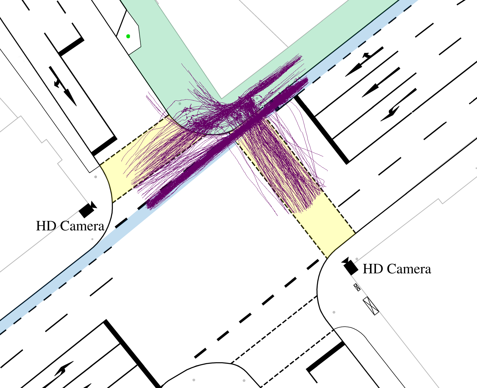
To train and test the algorithms, we created a dataset containing 394 scenes of starting cyclists recorded at an urban intersection equipped with two HD cameras [13], with a frame rate of $50\text{\,}\mathrm{Hz}$, arranged in a wide angle stereo camera system (Fig. 1). The camera field of view covers a sidewalk (Fig. 1, green) with two pedestrian crossings (yellow) and a bicycle lane (blue).

The dataset consists of 49 male and female test subjects, who were instructed to move between certain points on the intersection, while following the traffic rules, which lead to 89 starting motions. Additionally, 305 starting motions of uninstructed cyclists were recorded at random times, resulting in 394 starting motions total. The set was divided with a 60-20-20 split into training, validation, and test data. The trajectories of the recorded cyclists are shown in Fig. 1 in purple.

To generate the input of the classifiers $x_{t}$ containing the MHIs, the head positions were labeled manually in every image. A region of interest (ROI) with a size large enough to enclose the cyclist including the bicycle was chosen and based on the head position used to crop the images of the past $N$ time steps, which are used to create the MHI, as described in Sec. II-B. The used ROI size is 192$\times$$160\text{\,}\mathrm{px}$.

The output of the classifier $\hat{y}_{t}$ contains the class probabilities $P_{waiting}$ and $P_{moving}$. Additionally, an auxiliary class starting for evaluation of the classifier is introduced. The labels were created manually and are defined as follows: An image is labeled waiting, while neither the wheel of the bicycle is moving, nor the cyclist is performing a movement which leads to a starting motion. Every frame between the first visible movement of the cyclist that leads to a starting motion and the first movement of the bicycle wheel is labeled as starting. Finally, every frame after the first movement of the bicycle wheel is labeled moving. For training, starting and moving are merged into one class.

II-B Generation of Motion History Images

In this section, we describe how the MHIs used to classify the starting motions are generated. The generation is depicted in Fig. 2. In the first step, an ROI enclosing the detected cyclist and bicycle is created on the camera image which contains the side view of the cyclist (Fig. 2, left). The image is cropped to the size of the ROI and fed to a semantic segmentation. For the segmentation, the ResNet from [14] pretrained on the CoCo dataset [15] and trained on the PASCAL VOC dataset [16] is used to assign classes to every pixel in the image. We use the VOC dataset over the Cityscapes dataset [17], because it contains images of cyclists from different angles, which are very close to our stationary camera dataset, whereas the Cityscapes dataset consists solely of images recorded from a car. The segmentation outputs 20 classes of which the classes person, bicycle, and motorbike are used to generate the silhouettes of cyclists and bicycles (Fig. 2, second from left). The class motorbike is used, since parts of the bicycle are often misclassified as motorcycle. The image is binarized by setting these three classes to one and the other classes to zero. To generate the MHI (Fig. 2, right), binarized images $I(u,v,t)$ at different time steps $t$ are multiplied by a decay value $\tau(t)=\frac{N-t}{N}$, where $N$ is the number of past images used and $t$ is the $t^{th}$ image in the sequence, where $t=0$ is the most recent image. The decayed images are then stacked using Algorithm 1.

Algorithm 1 MHI Generation

1:$I(u,v,t)\leftarrow$ sequence of images with time step t and pixel positions $u$ and $v$, where $I(u,v,0)$ is the most recent image

2:$N\leftarrow$ number of time steps in $I(u,v,t)$

3:$W\leftarrow$ image width

4:$H\leftarrow$ image height

5:$MHI(u,v):=0$

6:for $t=N-1\text{ to }0$ do$\triangleright$ iterate over all images, start with oldest

7:     $\tau(t)=\frac{N-t}{N}$$\triangleright$ calculate decay value $\tau$

8:     for $u=0\text{ to }W-1$ do$\triangleright$ go through all pixels

9:         for $v=0\text{ to }H-1$ do

10:              if $I(u,v,t)==1$ then $\triangleright$ update MHI

11:                  $MHI(u,v)=\tau(t)\cdot I(u,v,t)$

12:              end if

13:         end for

14:     end for

15:end for

II-C MCHOG Detector

To detect cyclist starting motions using MCHOG, the method used to detect pedestrian motions described in [4] is adapted to cyclists. The MCHOG descriptor is generated by computing the magnitude and orientation of the gradients in the MHI, dividing the image into cells and computing cell histograms. In contrast to the original implementation of the HOG descriptor [18], a block normalization of cells is not performed, as it reduces the local differences between neighboring cells. The concatenated cell histograms result in the MCHOG descriptor, which is used as input of a linear SVM classifier. The HOG descriptors are computed on MHIs. To reduce the number of features, the MHIs are resized to 128$\times$$96\text{\,}\mathrm{px}$. To generate probability outputs from the SVM, probability calibration was performed using Platt’s algorithm [19].

II-D Deep Residual Network Detector

In this section, we describe the detection of starting motions using a ResNet architecture which was first introduced by He et al. in [11]. The authors showed, that their network is easier to train and generates a higher accuracy compared to conventional CNNs, by addressing a degradation problem, where adding more layers to conventional deep models leads to a higher training error. They introduced residual building blocks (Fig. 3, upper right), where instead of directly modeling a target function $H(x)$ using a non linear model $F(x)$, they created a bypass and added the input to the output $F(x)+x$. Thus $F(x)$ models the residual of $H(x)$. One explanation for the degradation problem is that it is difficult to model identities with non linear layers. Using a residual layer, the identity can be modeled by driving the weights to zero. By stacking residual blocks, the authors were able to train a network with 152 layers, which produced substantially better results than shallower networks.

Figure 3: ResNet architecture with a reduction layer (bottom right) and residual blocks (top right).

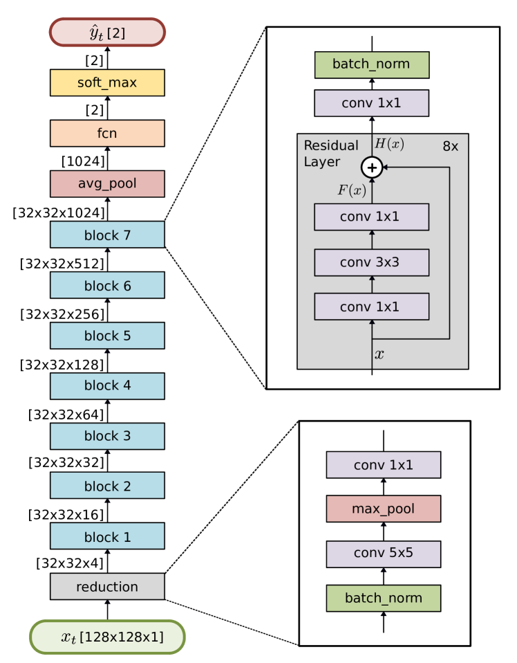
Our network architecture, which is described in Fig. 3, is based on the architecture in [11]. The MHI, resized to 128$\times$$128\text{\,}\mathrm{px}$, is used as input where a reduction layer (Fig. 3, lower right) consisting of batch normalization, a 5$\times$5 convolution, and a max pooling layer is used to reduce the image dimension. A 1$\times$1 convolution is applied to generate four feature maps. The feature maps are then passed to a residual block, which is described in Fig. 3 on the upper right. In our network, a residual block consists of eight residual layers with bottleneck architecture to reduce the computational effort, followed by a 1$\times$1 convolution to generate the output feature maps and a batch normalization layer. After seven residual blocks an average pooling is applied to receive a feature vector containing 1024 features, which are classified by a fully connected layer (fcn) with softmax activation to generate probabilities. To speed up the training process, batch normalization layers are added at the network input and after every residual block.

II-E Evaluation Method

To evaluate our algorithms, we used the recorded dataset described in Sec. II-A, i.e., the evaluation was done offline.

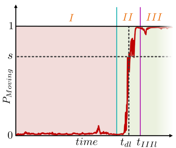
The performance of both detectors was determined by a scene wise evaluation, where one scene starts after the cyclists stopped and ends when the cyclist leaves the field of view of the side view camera. Fig. 4 shows an exemplary output of a scene, where $P_{Moving}$ (red line) is plotted over time. Phase $I$ is the waiting phase, phase $II$ and $III$ are starting and moving phases, respectively. A desired output of the detector is shown in Fig. 4, $P_{Moving}$ maintains a low value during Phase $I$, increases in phase $II$, and remains at a high level during phase $III$. A starting movement is detected when $P_{moving}$ reaches a certain threshold ($s$ in Fig. 4). A scene is rated as true positive, if the threshold is reached in phase $II$ or $III$. If the threshold is reached during phase $I$, the scene is rated as false positive. If the threshold is never reached, it is rated as false negative. We do not consider true negatives, since every scene results in moving.

Using this method, we calculate the $precision$ and the $F_{1}$-score for thresholds between zero and one with a step size of 0.02. Additionally, we evaluate the detection time by calculating the mean time difference $\overline{\delta_{t}}$ between the detection time $t_{dl}$ and the start time of phase $III$ $t_{IIIl}$ in the $l^{th}$ sequence of all true positives over all $L$ sequences (Eq. 1), where smaller values indicate faster detection.

$$\overline{\delta_{t}}=\frac{1}{L}\cdot\sum_{l=1}^{L}(t_{dl}-t_{IIIl})$$ (1)

Figure 4: Exemplary classification output of a scene, with moving probability $P_{Moving}$ (red), labeled starting time (blue), and labeled moving time $t_{IIIl}$ (purple). A chosen threshold $s$, leads to detection time $t_{dl}$.

III Experimental results

This section describes the evaluation of the proposed methods and compares their results.

Figure 5: $F_{1}$-scores (blue), $precision$ (red), and mean detection time $\overline{\delta_{t}}$ over probability thresholds of MCHOG (left) and ResNet (right).

TABLE I: Values used in MCHOG parameter sweep.

Param.	cell size x	cell size y	nbins	$C$ param
Value	$\{8,16,32\}$	$\{8,16,32\}$	$\{6,12,16\}$	$\{2^{c}|-9<c<5:c\in\mathbb{N}\}$

III-A MCHOG Results

In this section, we present the results of the detection using MCHOG in combination with an SVM. We performed a grid search over the cell size in x and y direction, the number of bins in a histogram and the $C$ parameter of the SVM. The values used in the parameter sweep can be found in Tab. I. The dataset described in Sec. II-A was used for training, validation and test.

We generated the $F_{1}$-score and the mean detection time $\overline{\delta_{t}}$ needed to achieve the highest $F_{1}$-score for every parameter configuration using the validation set. The five best and three worst validation results are shown in Tab. II. It shows that four of the five best results have the same MCHOG parameters and only differ in the $C$ parameter of the SVM. Furthermore, the parameter sweep yielded 51 detectors that reached an $F_{1}$-score of 100%, where $\overline{\delta_{t}}$ ranges from $0.565\text{\,}\mathrm{s}$ for the fastest detector to $1.11\,s$ for the slowest detector. The classifiers with large cell size in y direction and low number of histogram bins yielded the lowest $F_{1}$-scores.

TABLE II: Validation results from MCHOG parameter sweep.

$F_{1}$	$\overline{\delta_{t}}$	cell size x	cell size y	nbins	$C$ param
1.0	$0.565\text{\,}\mathrm{s}$	32	8	18	0.03125
1.0	$0.578\text{\,}\mathrm{s}$	32	8	18	0.0625
1.0	$0.586\text{\,}\mathrm{s}$	32	8	18	0.125
1.0	$0.608\text{\,}\mathrm{s}$	8	8	12	0.25
1.0	$0.609\text{\,}\mathrm{s}$	32	8	18	0.25
…	…	…	…	…	…
0.915	$0.968\text{\,}\mathrm{s}$	32	32	6	4
0.915	$0.968\text{\,}\mathrm{s}$	32	32	6	2
0.915	$0.968\text{\,}\mathrm{s}$	32	32	6	8

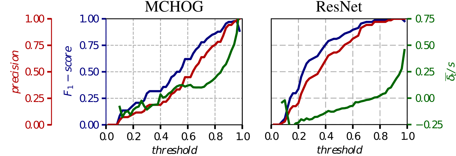
To generate the test results, the detector with pareto-optimal validation scores was chosen, i.e., greatest $F_{1}$-score and lowest $\overline{\delta_{t}}$. Fig. 5 (left) shows the overall results of the detector. To generate the plot, the $F_{1}$-score, the $precision$ and $\overline{\delta_{t}}$ were generated for different probability thresholds (as described in Sec. II-E) and plotted over thresholds from zero to one. Our evaluation shows that the detector reaches an $F_{1}$-score of 90% $0.274\text{\,}\mathrm{s}$ after the first movement of the bicycle wheel and the highest $F_{1}$-score of 97.8% is reached after $0.506\text{\,}\mathrm{s}$.

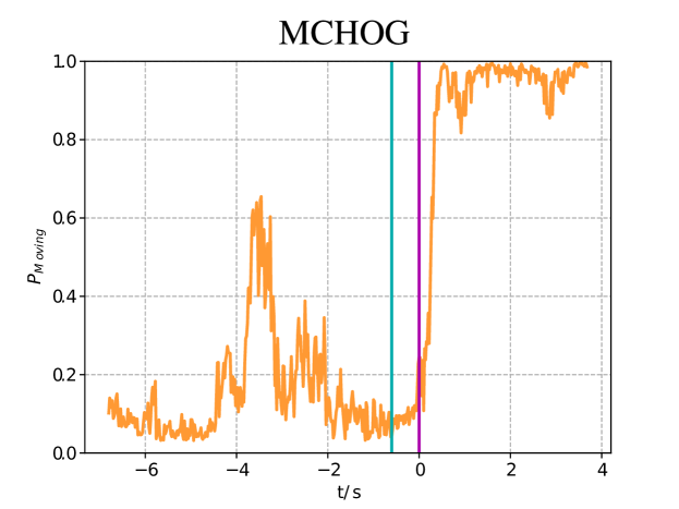
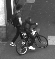
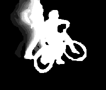
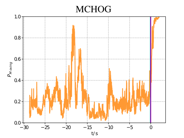
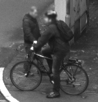
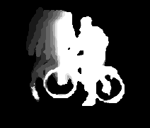
The classifier is robust against movements of the cyclist that do not lead to starting motion, however strongly reacts to movements of pedestrians passing in the background. Fig. 6 and Fig. 8 show two example classifications with pedestrians moving in the background of the waiting cyclists, which leads to an increase in $P_{Moving}$. Fig. 7 and 9 show the passing pedestrians in the camera image and the corresponding MHI. The peak in $P_{Moving}$ is reached when the pedestrian is occluded by the cyclist and only the motion contour of the pedestrian is visible, making it appear that the motion contour belongs to the cyclist. The second peak in Fig. 8 between $-8\text{\,}\mathrm{s}$ and $-11\text{\,}\mathrm{s}$ results from a strong forward movement of the cyclist and the bicycle.

Figure 6: Example detection 1: Moving probabilities of MCHOG (top) and ResNet (bottom) detection with crossing pedestrian between $-5\text{\,}\mathrm{s}$ and $-2\text{\,}\mathrm{s}$.

Figure 7: Example detection 1: Pedestrian passing behind cyclist.

Figure 8: Example detection 2: Moving probabilities of MCHOG (top) and ResNet (bottom) detection with crossing pedestrian between $-20\text{\,}\mathrm{s}$ and $-15\text{\,}\mathrm{s}$.

Figure 9: Example detection 2: Pedestrian passing close behind cyclist.

III-B Residual Network Results

The ResNet detector was trained using the same dataset as the MCHOG classifier. As optimizer we used RMSProp in combination with a cross entropy loss function and a batch size of 10. The training was executed on an NVIDIA GTX 1080 Ti GPU using Tensorflow [20]. The network was trained for 120,000 iterations.

To choose the best network, a validation step was performed every 250 iterations, where the $F_{1}$-score and $\overline{\delta_{t}}$ were calculated for the validation set. The network with the best validation scores reaches an $F_{1}$-score of 100% with $\overline{\delta_{t}}=$$0.175\text{\,}\mathrm{s}$ at iteration 66,000 and was used to create the test results.

The overall results are shown in Fig. 5 (right). The classifier reaches an $F_{1}$-score score of 90$\%$ after $-0.038\text{\,}\mathrm{s}$ and the highest $F_{1}$-score of 100% is reached after $0.144\text{\,}\mathrm{s}$.

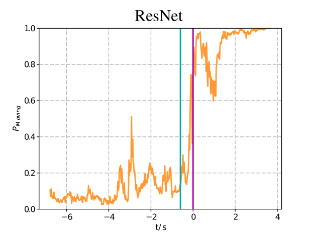
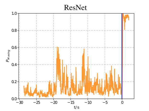
Like the MCHOG classifier, the ResNet is not influenced by small movements of the cyclist during the waiting phase. Scenes with pedestrians passing in the background of the cyclists result in an increase of $P_{Moving}$, however, compared to the MCHOG, the ResNet does not react as significantly. Additionally, the ResNet outperforms the MCHOG when it comes to detection time. Concerning the detectors with the best $F_{1}$-scores, the ResNet is able to detect starting motions $0.362\text{\,}\mathrm{s}$ earlier on average, compared to the MCHOG.

IV Conclusions and Future Work

In this article, we presented two methods based on MHIs to detect starting motions of cyclists. The methods were tested in real world scenarios at an urban intersection. We adapted an existing method, which uses MCHOG descriptors and an SVM, to detect motions of pedestrians to cyclists and presented a new approach by using ResNet to detect starting motions.

Using the MCHOG, we achieve an $F_{1}$-score of 97.8% after $0.506\text{\,}\mathrm{s}$. The ResNet approach outperforms the MCHOG in both robustness against false positives and detection time with a maximum $F_{1}$-score of 100% after $0.144\text{\,}\mathrm{s}$ on average.

Our future work will focus on how the developed methods can be used to further improve trajectories forecast algorithms. We also intend to adapt our method to moving vehicles. Furthermore, we will investigate how the methods can be utilized in a cooperative way between different traffic participants to generate a comprehensive model of the environment.

V Acknowledgment

This work results from the project DeCoInt², supported by the German Research Foundation (DFG) within the priority program SPP 1835: “Kooperativ interagierende Automobile”, grant numbers DO 1186/1-1 and SI 674/11-1. Additionally, the work is supported by “Zentrum Digitalisierung Bayern”.

References

- [1] World Health Organization, “Global Status Report on Road Safety 2015,” 2015. [Online]. Available: http://www.who.int/violence_injury_prevention/road_safety_status/2015/en/
- [2] C. Keller, C. Hermes, and D. Gavrila, “Will the pedestrian cross? probabilistic path prediction based on learned motion features,” in Pattern Recognition. Springer, 2011, vol. 6835, pp. 386–395.
- [3] M. Bieshaar, S. Zernetsch, M. Depping, B. Sick, and K. Doll, “Cooperative starting intention detection of cyclists based on smart devices and infrastructure,” in International Conference on Intelligent Transportation Systems (ITSC), Yokohama, 2017.
- [4] S. Koehler, M. Goldhammer, S. Bauer, S. Zecha, K. Doll, U. Brunsmann, and K. Dietmayer, “Stationary detection of the pedestrian’s intention at intersections,” IEEE Intelligent Transportation Systems Magazine, vol. 5, no. 4, pp. 87–99, 2013.
- [5] R. Quintero, I. Parra, J. Lorenzo, D. Fernández-Llorca, and M. A. Sotelo, “Pedestrian intention recognition by means of a hidden markov model and body language,” in International Conference on Intelligent Transportation Systems (ITSC), Yokohama, 2017.
- [6] C. Keller and D. Gavrila, “Will the pedestrian cross? a study on pedestrian path prediction,” Intelligent Transportation Systems, IEEE Transactions on, vol. 15, no. 2, pp. 494–506, 2014.
- [7] S. Koehler, M. Goldhammer, K. Zindler, K. Doll, and K. Dietmayer, “Stereo-vision-based pedestrian’s intention detection in a moving vehicle,” in International Conference on Intelligent Transportation Systems (ITSC), Gran Canaria, Sept 2015, pp. 2317–2322.
- [8] R. Quintero, I. Parra, D. F. Llorca, and M. A. Sotelo, “Pedestrian intention and pose prediction through dynamical models and behaviour classification,” in International Conference on Intelligent Transportation Systems (ITSC), Anchorage, 2015, pp. 83–88.
- [9] E. A. I. Pool, J. F. P. Kooij, and D. M. Gavrila, “Using road topology to improve cyclist path prediction,” in IEEE Intelligent Vehicles Symposium (IV), Redondo Beach, June 2017, pp. 289–296.
- [10] A. Hubert, S. Zernetsch, K. Doll, and B. Sick, “Cyclists’ starting behavior at intersections,” in Intelligent Vehicles Symposium (IV), June 2017, pp. 1071–1077.
- [11] K. He, X. Zhang, S. Ren, and J. Sun, “Deep residual learning for image recognition,” in IEEE Conference on Computer Vision and Pattern Recognition (CVPR), Las Vegas, 2016, pp. 770–778.
- [12] O. Russakovsky, J. Deng, H. Su, J. Krause, S. Satheesh, S. Ma, Z. Huang, A. Karpathy, A. Khosla, M. Bernstein, A. C. Berg, and L. Fei-Fei, “ImageNet Large Scale Visual Recognition Challenge,” International Journal of Computer Vision (IJCV), vol. 115, no. 3, pp. 211–252, 2015.
- [13] M. Goldhammer, E. Strigel, D. Meissner, U. Brunsmann, K. Doll, and K. Dietmayer, “Cooperative multi sensor network for traffic safety applications at intersections,” in International Conference on Intelligent Transportation Systems (ITSC), Anchorage, 2012, pp. 1178–1183.
- [14] Z. Wu, C. Shen, and A. van den Hengel, “Wider or deeper: Revisiting the resnet model for visual recognition,” arXiv:1611.10080, 2016.
- [15] T.-Y. Lin, M. Maire, S. Belongie, J. Hays, P. Perona, D. Ramanan, P. Dollár, and C. L. Zitnick, Microsoft COCO: Common Objects in Context. Cham: Springer International Publishing, 2014, pp. 740–755.
- [16] M. Everingham, L. Van Gool, C. K. I. Williams, J. Winn, and A. Zisserman, “The pascal visual object classes (voc) challenge,” International Journal of Computer Vision, vol. 88, no. 2, pp. 303–338, 2010.
- [17] M. Cordts, M. Omran, S. Ramos, T. Rehfeld, M. Enzweiler, R. Benenson, U. Franke, S. Roth, and B. Schiele, “The cityscapes dataset for semantic urban scene understanding,” in Proc. of the IEEE Conference on Computer Vision and Pattern Recognition (CVPR), Las Vegas, 2016.
- [18] N. Dalal and B. Triggs, “Histograms of Oriented Gradients for Human Detection,” in IEEE Conference on Computer Vision and Pattern Recognition (CVPR), San Diego, 2005, pp. 886–893.
- [19] J. C. Platt, “Probabilistic outputs for support vector machines and comparisons to regularized likelihood methods,” in Advances in Large Margin Classifiers. MIT Press, 1999, pp. 61–74.
- [20] M. Abadi et al., “TensorFlow: Large-scale machine learning on heterogeneous systems,” 2015, software available from tensorflow.org. [Online]. Available: https://www.tensorflow.org/