Computational Optimal Transport

Gabriel Peyré
CNRS and DMA
   ENS    Marco Cuturi
Google and CREST
   ENSAE
Abstract

Optimal transport (OT) theory can be informally described using the words of the French mathematician Gaspard Monge (1746–1818): A worker with a shovel in hand has to move a large pile of sand lying on a construction site. The goal of the worker is to erect with all that sand a target pile with a prescribed shape (for example, that of a giant sand castle). Naturally, the worker wishes to minimize her total effort, quantified for instance as the total distance or time spent carrying shovelfuls of sand. Mathematicians interested in OT cast that problem as that of comparing two probability distributions—two different piles of sand of the same volume. They consider all of the many possible ways to morph, transport or reshape the first pile into the second, and associate a “global” cost to every such transport, using the “local” consideration of how much it costs to move a grain of sand from one place to another. Mathematicians are interested in the properties of that least costly transport, as well as in its efficient computation. That smallest cost not only defines a distance between distributions, but it also entails a rich geometric structure on the space of probability distributions. That structure is canonical in the sense that it borrows key geometric properties of the underlying “ground” space on which these distributions are defined. For instance, when the underlying space is Euclidean, key concepts such as interpolation, barycenters, convexity or gradients of functions extend naturally to the space of distributions endowed with an OT geometry.

OT has been (re)discovered in many settings and under different forms, giving it a rich history. While Monge’s seminal work was motivated by an engineering problem, Tolstoi in the 1920s and Hitchcock, Kantorovich and Koopmans in the 1940s established its significance to logistics and economics. Dantzig solved it numerically in 1949 within the framework of linear programming, giving OT a firm footing in optimization. OT was later revisited by analysts in the 1990s, notably Brenier, while also gaining fame in computer vision under the name of earth mover’s distances. Recent years have witnessed yet another revolution in the spread of OT, thanks to the emergence of approximate solvers that can scale to large problem dimensions. As a consequence, OT is being increasingly used to unlock various problems in imaging sciences (such as color or texture processing), graphics (for shape manipulation) or machine learning (for regression, classification and generative modeling).

This paper reviews OT with a bias toward numerical methods, and covers the theoretical properties of OT that can guide the design of new algorithms. We focus in particular on the recent wave of efficient algorithms that have helped OT find relevance in data sciences. We give a prominent place to the many generalizations of OT that have been proposed in but a few years, and connect them with related approaches originating from statistical inference, kernel methods and information theory. All of the figures can be reproduced using code made available in a companion website111https://optimaltransport.github.io/. This website hosts the book project Computational Optimal Transport. You will also find slides and computational resources.

@article{COTFNT,
year = {2019},
volume = {11},
journal = {Foundations and Trends in Machine Learning},
title = {Computational Optimal Transport},
number = {5-6},
pages = {355--607}
author = {Gabriel Peyr\’e and Marco Cuturi}
}

Chapter 1 Introduction

The shortest path principle guides most decisions in life and sciences: When a commodity, a person or a single bit of information is available at a given point and needs to be sent at a target point, one should favor using the least possible effort. This is typically reached by moving an item along a straight line when in the plane or along geodesic curves in more involved metric spaces. The theory of optimal transport generalizes that intuition in the case where, instead of moving only one item at a time, one is concerned with the problem of moving simultaneously several items (or a continuous distribution thereof) from one configuration onto another. As schoolteachers might attest, planning the transportation of a group of individuals, with the constraint that they reach a given target configuration upon arrival, is substantially more involved than carrying it out for a single individual. Indeed, thinking in terms of groups or distributions requires a more advanced mathematical formalism which was first hinted at in the seminal work of Monge (1781). Yet, no matter how complicated that formalism might look at first sight, that problem has deep and concrete connections with our daily life. Transportation, be it of people, commodities or information, very rarely involves moving only one item. All major economic problems, in logistics, production planning or network routing, involve moving distributions, and that thread appears in all of the seminal references on optimal transport. Indeed Tolstoı (1930)Hitchcock (1941) and Kantorovich (1942) were all guided by practical concerns. It was only a few years later, mostly after the 1980s, that mathematicians discovered, thanks to the works of Brenier (1991) and others, that this theory provided a fertile ground for research, with deep connections to convexity, partial differential equations and statistics. At the turn of the millenium, researchers in computer, imaging and more generally data sciences understood that optimal transport theory provided very powerful tools to study distributions in a different and more abstract context, that of comparing distributions readily available to them under the form of bags-of-features or descriptors.

Several reference books have been written on optimal transport, including the two recent monographs by Villani (2003; 2009), those by Rachev and Rüschendorf (1998a; 1998b) and more recently that by Santambrogio (2015). As exemplified by these books, the more formal and abstract concepts in that theory deserve in and by themselves several hundred pages. Now that optimal transport has gradually established itself as an applied tool (for instance, in economics, as put forward recently by Galichon (2016)), we have tried to balance that rich literature with a computational viewpoint, centered on applications to data science, notably imaging sciences and machine learning. We follow in that sense the motivation of the recent review by Kolouri et al. (2017) but try to cover more ground. Ultimately, our goal is to present an overview of the main theoretical insights that support the practical effectiveness of OT and spend more time explaining how to turn these insights into fast computational schemes. The main body of Chapters 2, 3, 4, 9, and 10 is devoted solely to the study of the geometry induced by optimal transport in the space of probability vectors or discrete histograms. Targeting more advanced readers, we also give in the same chapters, in light gray boxes, a more general mathematical exposition of optimal transport tailored for discrete measures. Discrete measures are defined by their probability weights, but also by the location at which these weights are defined. These locations are usually taken in a continuous metric space, giving a second important degree of freedom to model random phenomena. Lastly, the third and most technical layer of exposition is indicated in dark gray boxes and deals with arbitrary measures that need not be discrete, and which can have in particular a density w.r.t. a base measure. This is traditionally the default setting for most classic textbooks on OT theory, but one that plays a less important role in general for practical applications. Chapters 5 to 8 deal with the interplay between continuous and discrete measures and are thus targeting a more mathematically inclined audience.

The field of computational optimal transport is at the time of this writing still an extremely active one. There are therefore a wide variety of topics that we have not touched upon in this survey. Let us cite in no particular order the subjects of distributionally robust optimization (Shafieezadeh Abadeh et al., 2015; Esfahani and Kuhn, 2018; Lee and Raginsky, 2018; GAO et al., 2018), in which parameter estimation is carried out by minimizing the worst posssible empirical risk of any data measure taken within a certain Wasserstein distance of the input data; convergence of the Langevin Monte Carlo sampling algorithm in the Wasserstein geometry (Dalalyan and Karagulyan, 2017; Dalalyan, 2017; Bernton, 2018); other numerical methods to solve OT with a squared Euclidian cost in low-dimensional settings using the Monge-Ampère equation (Froese and Oberman, 2011; Benamou et al., 2014; Sulman et al., 2011) which are only briefly mentioned in Remark 2.25.

Notation

  • ndelimited-⟦⟧𝑛\llbracket n\rrbracket: set of integers {1,,n}1𝑛\{1,\dots,n\}.

  • 𝟙n,msubscriptdouble-struck-𝟙𝑛𝑚\mathbb{1}_{n,m}: matrix of n×msuperscript𝑛𝑚\mathbb{R}^{n\times m} with all entries identically set to 111. 𝟙nsubscriptdouble-struck-𝟙𝑛\mathbb{1}_{n}: vector of ones.

  • 𝕀nsubscript𝕀𝑛\mathbb{I}_{n}: identity matrix of size n×n𝑛𝑛n\times n.

  • For un𝑢superscript𝑛u\in\mathbb{R}^{n}, diag(u)diag𝑢\operatorname{diag}(u) is the n×n𝑛𝑛n\times n matrix with diagonal u𝑢u and zero otherwise.

  • ΣnsubscriptΣ𝑛\Sigma_{n}: probability simplex with n𝑛n bins, namely the set of probability vectors in +nsubscriptsuperscript𝑛\mathbb{R}^{n}_{+}.

  • (a,b)ab(\mathrm{\textbf{a}},\mathrm{\textbf{b}}): histograms in the simplices Σn×ΣmsubscriptΣ𝑛subscriptΣ𝑚\Sigma_{n}\times\Sigma_{m}.

  • (α,β)𝛼𝛽(\alpha,\beta): measures, defined on spaces (𝒳,𝒴)𝒳𝒴(\mathcal{X},\mathcal{Y}).

  • dαdβd𝛼d𝛽\frac{\mathrm{d}\alpha}{\mathrm{d}\beta}: relative density of a measure α𝛼\alpha with respect to β𝛽\beta.

  • ρα=dαdxsubscript𝜌𝛼d𝛼d𝑥\rho_{\alpha}=\frac{\mathrm{d}\alpha}{\mathrm{d}x}: density of a measure α𝛼\alpha with respect to Lebesgue measure.

  • (α=iaiδxi,β=jbjδyj)formulae-sequence𝛼subscript𝑖subscripta𝑖subscript𝛿subscript𝑥𝑖𝛽subscript𝑗subscriptb𝑗subscript𝛿subscript𝑦𝑗(\alpha=\sum_{i}\mathrm{\textbf{a}}_{i}\delta_{x_{i}},\beta=\sum_{j}\mathrm{\textbf{b}}_{j}\delta_{y_{j}}): discrete measures supported on x1,,xn𝒳subscript𝑥1subscript𝑥𝑛𝒳x_{1},\dots,x_{n}\in\mathcal{X} and y1,,ym𝒴subscript𝑦1subscript𝑦𝑚𝒴y_{1},\dots,y_{m}\in\mathcal{Y}.

  • c(x,y)𝑐𝑥𝑦c(x,y): ground cost, with associated pairwise cost matrix Ci,j=(c(xi,yj))i,jsubscriptC𝑖𝑗subscript𝑐subscript𝑥𝑖subscript𝑦𝑗𝑖𝑗\mathrm{\textbf{C}}_{i,j}=(c(x_{i},y_{j}))_{i,j} evaluated on the support of α,β𝛼𝛽\alpha,\beta.

  • π𝜋\pi: coupling measure between α𝛼\alpha and β𝛽\beta, namely such that for any A𝒳,π(A×𝒴)=α(A)formulae-sequence𝐴𝒳𝜋𝐴𝒴𝛼𝐴A\subset\mathcal{X},\pi(A\times\mathcal{Y})=\alpha(A), and for any subset B𝒴,π(𝒳×B)=β(B)formulae-sequence𝐵𝒴𝜋𝒳𝐵𝛽𝐵B\subset\mathcal{Y},\pi(\mathcal{X}\times B)=\beta(B). For discrete measures π=i,jPi,jδ(xi,yj)𝜋subscript𝑖𝑗subscriptP𝑖𝑗subscript𝛿subscript𝑥𝑖subscript𝑦𝑗\pi=\sum_{i,j}\mathrm{\textbf{P}}_{i,j}\delta_{(x_{i},y_{j})}.

  • 𝒰(α,β)𝒰𝛼𝛽\mathcal{U}(\alpha,\beta): set of coupling measures, for discrete measures U(a,b)Uab\mathrm{\textbf{U}}(\mathrm{\textbf{a}},\mathrm{\textbf{b}}).

  • (c)𝑐\mathcal{R}(c): set of admissible dual potentials; for discrete measures R(C)RC\mathrm{\textbf{R}}(\mathrm{\textbf{C}}).

  • T:𝒳𝒴:𝑇𝒳𝒴T:\mathcal{X}\rightarrow\mathcal{Y}: Monge map, typically such that Tα=βsubscript𝑇𝛼𝛽T_{\sharp}\alpha=\beta.

  • (αt)t=01superscriptsubscriptsubscript𝛼𝑡𝑡01(\alpha_{t})_{t=0}^{1}: dynamic measures, with αt=0=α0subscript𝛼𝑡0subscript𝛼0\alpha_{t=0}=\alpha_{0} and αt=1=α1subscript𝛼𝑡1subscript𝛼1\alpha_{t=1}=\alpha_{1}.

  • v𝑣v: speed for Benamou–Brenier formulations; J=αv𝐽𝛼𝑣J=\alpha v: momentum.

  • (f,g)𝑓𝑔(f,g): dual potentials, for discrete measures (f,g)fg(\mathrm{\textbf{f}},\mathrm{\textbf{g}}) are dual variables.

  • (u,v)=def.(ef/ε,eg/ε)superscriptdef.uvsuperscript𝑒f𝜀superscript𝑒g𝜀(\mathrm{\textbf{u}},\mathrm{\textbf{v}})\stackrel{{\scriptstyle\mbox{\tiny def.}}}{{=}}(e^{\mathrm{\textbf{f}}/\varepsilon},e^{\mathrm{\textbf{g}}/\varepsilon}): Sinkhorn scalings.

  • K=def.eC/εsuperscriptdef.Ksuperscript𝑒C𝜀\mathrm{\textbf{K}}\stackrel{{\scriptstyle\mbox{\tiny def.}}}{{=}}e^{-\mathrm{\textbf{C}}/\varepsilon}: Gibbs kernel for Sinkhorn.

  • s𝑠s: flow for 𝒲1subscript𝒲1\operatorname{\mathcal{W}}_{1}-like problem (optimization under divergence constraints).

  • LC(a,b)subscriptLCab\mathrm{L}_{\mathrm{\textbf{C}}}(\mathrm{\textbf{a}},\mathrm{\textbf{b}}) and c(α,β)subscript𝑐𝛼𝛽\mathcal{L}_{c}(\alpha,\beta): value of the optimization problem associated to the OT with cost C (histograms) and c𝑐c (arbitrary measures).

  • Wp(a,b)subscriptW𝑝ab\operatorname{\mathrm{W}}_{p}(\mathrm{\textbf{a}},\mathrm{\textbf{b}}) and 𝒲p(α,β)subscript𝒲𝑝𝛼𝛽\operatorname{\mathcal{W}}_{p}(\alpha,\beta): p𝑝p-Wasserstein distance associated to ground distance matrix D (histograms) and distance d𝑑d (arbitrary measures).

  • λΣS𝜆subscriptΣ𝑆\lambda\in\Sigma_{S}: weight vector used to compute the barycenters of S𝑆S measures.

  • ,\langle\cdot,\,\cdot\rangle: for the usual Euclidean dot-product between vectors; for two matrices of the same size A𝐴A and B𝐵B, A,B=def.tr(AB)superscriptdef.𝐴𝐵trsuperscript𝐴top𝐵\langle A,\,B\rangle\stackrel{{\scriptstyle\mbox{\tiny def.}}}{{=}}\operatorname{tr}(A^{\top}B) is the Frobenius dot-product.

  • fg(x,y)=def.f(x)+g(y)superscriptdef.direct-sum𝑓𝑔𝑥𝑦𝑓𝑥𝑔𝑦f\oplus g(x,y)\stackrel{{\scriptstyle\mbox{\tiny def.}}}{{=}}f(x)+g(y), for two functions f:𝒳,g:𝒴:𝑓𝒳𝑔:𝒴f:\mathcal{X}\rightarrow\mathbb{R},g:\mathcal{Y}\rightarrow\mathbb{R}, defines fg:𝒳×𝒴:direct-sum𝑓𝑔𝒳𝒴f\oplus g:\mathcal{X}\times\mathcal{Y}\rightarrow\mathbb{R}.

  • fg=def.f𝟙m+𝟙ngn×msuperscriptdef.direct-sumfgfsuperscriptsubscriptdouble-struck-𝟙𝑚topsubscriptdouble-struck-𝟙𝑛superscriptgtopsuperscript𝑛𝑚\mathrm{\textbf{f}}\oplus\mathrm{\textbf{g}}\stackrel{{\scriptstyle\mbox{\tiny def.}}}{{=}}\mathrm{\textbf{f}}\mathbb{1}_{m}^{\top}+\mathbb{1}_{n}\mathrm{\textbf{g}}^{\top}\in\mathbb{R}^{n\times m} for two vectors fnfsuperscript𝑛\mathrm{\textbf{f}}\in\mathbb{R}^{n}, gmgsuperscript𝑚\mathrm{\textbf{g}}\in\mathbb{R}^{m}.

  • αβtensor-product𝛼𝛽\alpha\otimes\beta is the product measure on 𝒳×𝒴𝒳𝒴\mathcal{X}\times\mathcal{Y}, i.e. 𝒳×𝒴g(x,y)d(αβ)(x,y)=def.𝒳×𝒴g(x,y)dα(x)dβ(y)superscriptdef.subscript𝒳𝒴𝑔𝑥𝑦dtensor-product𝛼𝛽𝑥𝑦subscript𝒳𝒴𝑔𝑥𝑦differential-d𝛼𝑥differential-d𝛽𝑦\int_{\mathcal{X}\times\mathcal{Y}}g(x,y)\mathrm{d}(\alpha\otimes\beta)(x,y)\stackrel{{\scriptstyle\mbox{\tiny def.}}}{{=}}\int_{\mathcal{X}\times\mathcal{Y}}g(x,y)\mathrm{d}\alpha(x)\mathrm{d}\beta(y).

  • ab=def.abn×msuperscriptdef.tensor-productabsuperscriptabtopsuperscript𝑛𝑚\mathrm{\textbf{a}}\otimes\mathrm{\textbf{b}}\stackrel{{\scriptstyle\mbox{\tiny def.}}}{{=}}\mathrm{\textbf{a}}\mathrm{\textbf{b}}^{\top}\in\mathbb{R}^{n\times m}.

  • uv=(uivi)ndirect-productuvsubscriptu𝑖subscriptv𝑖superscript𝑛\mathrm{\textbf{u}}\odot\mathrm{\textbf{v}}=(\mathrm{\textbf{u}}_{i}\mathrm{\textbf{v}}_{i})\in\mathbb{R}^{n} for (u,v)(n)2uvsuperscriptsuperscript𝑛2(\mathrm{\textbf{u}},\mathrm{\textbf{v}})\in(\mathbb{R}^{n})^{2}.

Chapter 2 Theoretical Foundations

This chapter describes the basics of optimal transport, introducing first the related notions of optimal matchings and couplings between probability vectors (a,b)ab(\mathrm{\textbf{a}},\mathrm{\textbf{b}}), generalizing gradually this computation to transport between discrete measures (α,β)𝛼𝛽(\alpha,\beta), to cover lastly the general setting of arbitrary measures. At first reading, these last nuances may be omitted and the reader can only focus on computations between probability vectors, namely histograms, which is the only requisite to implement algorithms detailed in Chapters 3 and 4. More experienced readers will reach a better understanding of the problem by considering the formulation that applies to arbitrary measures, and will be able to apply it for more advanced problems (e.g. in order to move positions of clouds of points, or in a statistical setting where points are sampled from continuous densities).

2.1 Histograms and Measures

We will use interchangeably the terms histogram and probability vector for any element aΣnasubscriptΣ𝑛\mathrm{\textbf{a}}\in\Sigma_{n} that belongs to the probability simplex

Σn=def.{a+n:i=1nai=1}.superscriptdef.subscriptΣ𝑛conditional-setasuperscriptsubscript𝑛superscriptsubscript𝑖1𝑛subscripta𝑖1\Sigma_{n}\stackrel{{\scriptstyle\mbox{\tiny def.}}}{{=}}\left\{\mathrm{\textbf{a}}\in\mathbb{R}_{+}^{n}\;:\;\sum_{i=1}^{n}\mathrm{\textbf{a}}_{i}=1\right\}.

A large part of this review focuses exclusively on the study of the geometry induced by optimal transport on the simplex.

Remark 2.1 (Discrete measures).
A discrete measure with weights a and locations x1,,xn𝒳subscript𝑥1subscript𝑥𝑛𝒳x_{1},\dots,x_{n}\in\mathcal{X} reads α=i=1naiδxi,𝛼superscriptsubscript𝑖1𝑛subscripta𝑖subscript𝛿subscript𝑥𝑖\alpha=\sum_{i=1}^{n}\mathrm{\textbf{a}}_{i}\delta_{x_{i}}, (2.1) where δxsubscript𝛿𝑥\delta_{x} is the Dirac at position x𝑥x, intuitively a unit of mass which is infinitely concentrated at location x𝑥x. Such a measure describes a probability measure if, additionally, aΣnasubscriptΣ𝑛\mathrm{\textbf{a}}\in\Sigma_{n} and more generally a positive measure if all the elements of vector a are nonnegative. To avoid degeneracy issues where locations with no mass are accounted for, we will assume when considering discrete measures that all the elements of a are positive.
Remark 2.2 (General measures).
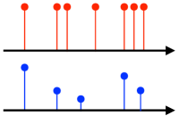
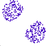
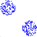
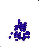
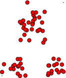
A convenient feature of OT is that it can deal with measures that are either or both discrete and continuous within the same framework. To do so, one relies on the set of Radon measures (𝒳)𝒳\mathcal{M}(\mathcal{X}) on the space 𝒳𝒳\mathcal{X}. The formal definition of that set requires that 𝒳𝒳\mathcal{X} is equipped with a distance, usually denoted d𝑑d, because one can access a measure only by “testing” (integrating) it against continuous functions, denoted f𝒞(𝒳)𝑓𝒞𝒳f\in\mathcal{C}(\mathcal{X}). Integration of f𝒞(𝒳)𝑓𝒞𝒳f\in\mathcal{C}(\mathcal{X}) against a discrete measure α𝛼\alpha computes a sum 𝒳f(x)dα(x)=i=1naif(xi).subscript𝒳𝑓𝑥differential-d𝛼𝑥superscriptsubscript𝑖1𝑛subscripta𝑖𝑓subscript𝑥𝑖\int_{\mathcal{X}}f(x)\mathrm{d}\alpha(x)=\sum_{i=1}^{n}\mathrm{\textbf{a}}_{i}f(x_{i}). More general measures, for instance on 𝒳=d𝒳superscript𝑑\mathcal{X}=\mathbb{R}^{d} (where d𝑑superscriptd\in\mathbb{N}^{*} is the dimension), can have a density dα(x)=ρα(x)dxd𝛼𝑥subscript𝜌𝛼𝑥d𝑥\mathrm{d}\alpha(x)=\rho_{\alpha}(x)\mathrm{d}x w.r.t. the Lebesgue measure, often denoted ρα=dαdxsubscript𝜌𝛼d𝛼d𝑥\rho_{\alpha}=\frac{\mathrm{d}\alpha}{\mathrm{d}x}, which means that h𝒞(d),dh(x)dα(x)=dh(x)ρα(x)dx.formulae-sequencefor-all𝒞superscript𝑑subscriptsuperscript𝑑𝑥differential-d𝛼𝑥subscriptsuperscript𝑑𝑥subscript𝜌𝛼𝑥differential-d𝑥\forall\,h\in\mathcal{C}(\mathbb{R}^{d}),\quad\int_{\mathbb{R}^{d}}h(x)\mathrm{d}\alpha(x)=\int_{\mathbb{R}^{d}}h(x)\rho_{\alpha}(x)\mathrm{d}x. An arbitrary measure α(𝒳)𝛼𝒳\alpha\in\mathcal{M}(\mathcal{X}) (which need not have a density nor be a sum of Diracs) is defined by the fact that it can be integrated against any continuous function f𝒞(𝒳)𝑓𝒞𝒳f\in\mathcal{C}(\mathcal{X}) and obtain 𝒳f(x)dα(x)subscript𝒳𝑓𝑥differential-d𝛼𝑥\int_{\mathcal{X}}f(x)\mathrm{d}\alpha(x)\in\mathbb{R}. If 𝒳𝒳\mathcal{X} is not compact, one should also impose that f𝑓f has compact support or at least has 00 limit at infinity. Measures are thus in some sense “less regular” than functions but more regular than distributions (which are dual to smooth functions). For instance, the derivative of a Dirac is not a measure. We denote +(𝒳)subscript𝒳\mathcal{M}_{+}(\mathcal{X}) the set of all positive measures on 𝒳𝒳\mathcal{X}. The set of probability measures is denoted +1(𝒳)superscriptsubscript1𝒳\mathcal{M}_{+}^{1}(\mathcal{X}), which means that any α+1(𝒳)𝛼superscriptsubscript1𝒳\alpha\in\mathcal{M}_{+}^{1}(\mathcal{X}) is positive, and that α(𝒳)=𝒳dα=1𝛼𝒳subscript𝒳differential-d𝛼1\alpha(\mathcal{X})=\int_{\mathcal{X}}\mathrm{d}\alpha=1. Figure 2.1 offers a visualization of the different classes of measures, beyond histograms, considered in this work.
Refer to caption Refer to caption Refer to caption Refer to caption
Discrete d=1𝑑1d=1 Discrete d=2𝑑2d=2 Density d=1𝑑1d=1 Density d=2𝑑2d=2
Figure 2.1: Schematic display of discrete distributions α=i=1naiδxi𝛼superscriptsubscript𝑖1𝑛subscripta𝑖subscript𝛿subscript𝑥𝑖\alpha=\sum_{i=1}^{n}\mathrm{\textbf{a}}_{i}\delta_{x_{i}} (red corresponds to empirical uniform distribution ai=1/nsubscripta𝑖1𝑛\mathrm{\textbf{a}}_{i}=1/n, and blue to arbitrary distributions) and densities dα(x)=ρα(x)dxd𝛼𝑥subscript𝜌𝛼𝑥d𝑥\mathrm{d}\alpha(x)=\rho_{\alpha}(x)\mathrm{d}x (in purple), in both one and two dimensions. Discrete distributions in one-dimension are displayed as stem plots (with length equal to aisubscripta𝑖\mathrm{\textbf{a}}_{i}) and in two dimensions using point clouds (in which case their radius might be equal to aisubscripta𝑖\mathrm{\textbf{a}}_{i} or, for a more visually accurate representation, their area).

2.2 Assignment and Monge Problem

Given a cost matrix (Ci,j)in,jmsubscriptsubscriptC𝑖𝑗𝑖delimited-⟦⟧𝑛𝑗delimited-⟦⟧𝑚(\mathrm{\textbf{C}}_{i,j})_{i\in\llbracket n\rrbracket,j\in\llbracket m\rrbracket}, assuming n=m𝑛𝑚n=m, the optimal assignment problem seeks for a bijection σ𝜎\sigma in the set Perm(n)Perm𝑛\mathrm{Perm}(n) of permutations of n𝑛n elements solving

minσPerm(n)1ni=1nCi,σ(i).𝜎Perm𝑛1𝑛superscriptsubscript𝑖1𝑛subscriptC𝑖𝜎𝑖\underset{\sigma\in\mathrm{Perm}(n)}{\min}\;\frac{1}{n}\sum_{i=1}^{n}\mathrm{\textbf{C}}_{i,\sigma(i)}. (2.2)

One could naively evaluate the cost function above using all permutations in the set Perm(n)Perm𝑛\mathrm{Perm}(n). However, that set has size n!𝑛n!, which is gigantic even for small n𝑛n. Consider, for instance, that such a set has more than 10100superscript1010010^{100} elements (Dantzig, 1983) when n𝑛n is as small as 70. That problem can therefore be solved only if there exist efficient algorithms to optimize that cost function over the set of permutations, which is the subject of §3.7.

Remark 2.3 (Uniqueness).

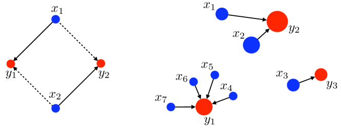
Note that the optimal assignment problem may have several optimal solutions. Suppose, for instance, that n=m=2𝑛𝑚2n=m=2 and that the matrix C is the pairwise distance matrix between the four corners of a 2-D square of side length 111, as represented in the left plot of Figure 2.2. In that case only two assignments exist, and they are both optimal.
Refer to caption
Figure 2.2: Left: blue dots from measure α𝛼\alpha and red dots from measure β𝛽\beta are pairwise equidistant. Hence, either matching σ=(1,2)𝜎12\sigma=(1,2) (full line) or σ=(2,1)𝜎21\sigma=(2,1) (dotted line) is optimal. Right: a Monge map can associate the blue measure α𝛼\alpha to the red measure β𝛽\beta. The weights αisubscript𝛼𝑖\alpha_{i} are displayed proportionally to the area of the disk marked at each location. The mapping here is such that T(x1)=T(x2)=y2𝑇subscript𝑥1𝑇subscript𝑥2subscript𝑦2T(x_{1})=T(x_{2})=y_{2}, T(x3)=y3𝑇subscript𝑥3subscript𝑦3T(x_{3})=y_{3}, whereas for 4i74𝑖74\leq i\leq 7 we have T(xi)=y1𝑇subscript𝑥𝑖subscript𝑦1T(x_{i})=y_{1}.
Remark 2.4 (Monge problem between discrete measures).
For discrete measures α=i=1naiδxiandβ=j=1mbjδyj,formulae-sequence𝛼superscriptsubscript𝑖1𝑛subscripta𝑖subscript𝛿subscript𝑥𝑖and𝛽superscriptsubscript𝑗1𝑚subscriptb𝑗subscript𝛿subscript𝑦𝑗\alpha=\sum_{i=1}^{n}\mathrm{\textbf{a}}_{i}\delta_{x_{i}}\quad\text{and}\quad\beta=\sum_{j=1}^{m}\mathrm{\textbf{b}}_{j}\delta_{y_{j}}, (2.3) the Monge problem (1781) seeks a map that associates to each point xisubscript𝑥𝑖x_{i} a single point yjsubscript𝑦𝑗y_{j} and which must push the mass of α𝛼\alpha toward the mass of β𝛽\beta, namely, such a map T:{x1,,xn}{y1,,ym}:𝑇subscript𝑥1subscript𝑥𝑛subscript𝑦1subscript𝑦𝑚T:\{x_{1},\dots,x_{n}\}\rightarrow\{y_{1},\dots,y_{m}\} must verify that jm,bj=i:T(xi)=yjai,\forall\,j\in\llbracket m\rrbracket,\quad\mathrm{\textbf{b}}_{j}=\sum_{i:T(x_{i})=y_{j}}\mathrm{\textbf{a}}_{i}, (2.4) which we write in compact form as Tα=βsubscript𝑇𝛼𝛽T_{\sharp}\alpha=\beta. Because all the elements of b are positive, that map is necessarily surjective. This map should minimize some transportation cost, which is parameterized by a function c(x,y)𝑐𝑥𝑦c(x,y) defined for points (x,y)𝒳×𝒴𝑥𝑦𝒳𝒴(x,y)\in\mathcal{X}\times\mathcal{Y}, min𝑇{ic(xi,T(xi)):Tα=β}.𝑇conditional-setsubscript𝑖𝑐subscript𝑥𝑖𝑇subscript𝑥𝑖subscript𝑇𝛼𝛽\underset{T}{\min}\;\left\{\sum_{i}c(x_{i},T(x_{i}))\;:\;T_{\sharp}\alpha=\beta\right\}. (2.5) Such a map between discrete points can be of course encoded, assuming all x𝑥x’s and y𝑦y’s are distinct, using indices σ:nm\sigma:\llbracket n\rrbracket\rightarrow\llbracket m\rrbracket so that j=σ(i)𝑗𝜎𝑖j=\sigma(i), and the mass conservation is written as iσ1(j)ai=bj,subscript𝑖superscript𝜎1𝑗subscripta𝑖subscriptb𝑗\sum_{i\in\sigma^{-1}(j)}\mathrm{\textbf{a}}_{i}=\mathrm{\textbf{b}}_{j}, where the inverse σ1(j)superscript𝜎1𝑗\sigma^{-1}(j) is to be understood as the preimage set of j𝑗j. In the special case when n=m𝑛𝑚n=m and all weights are uniform, that is, ai=bj=1/nsubscripta𝑖subscriptb𝑗1𝑛\mathrm{\textbf{a}}_{i}=\mathrm{\textbf{b}}_{j}=1/n, then the mass conservation constraint implies that T𝑇T is a bijection, such that T(xi)=yσ(i)𝑇subscript𝑥𝑖subscript𝑦𝜎𝑖T(x_{i})=y_{\sigma(i)}, and the Monge problem is equivalent to the optimal matching problem (2.2), where the cost matrix is Ci,j=def.c(xi,yj).superscriptdef.subscriptC𝑖𝑗𝑐subscript𝑥𝑖subscript𝑦𝑗\mathrm{\textbf{C}}_{i,j}\stackrel{{\scriptstyle\mbox{\tiny def.}}}{{=}}c(x_{i},y_{j}). When nm𝑛𝑚n\neq m, note that, optimality aside, Monge maps may not even exist between a discrete measure to another. This happens when their weight vectors are not compatible, which is always the case when the target measure has more points than the source measure, n<m𝑛𝑚n<m. For instance, the right plot in Figure 2.2 shows an (optimal) Monge map between α𝛼\alpha and β𝛽\beta, but there is no Monge map from β𝛽\beta to α𝛼\alpha.
Remark 2.5 (Push-forward operator).
For a continuous map T:𝒳𝒴:𝑇𝒳𝒴T:\mathcal{X}\rightarrow\mathcal{Y}, we define its corresponding push-forward operator T:(𝒳)(𝒴):subscript𝑇𝒳𝒴T_{\sharp}:\mathcal{M}(\mathcal{X})\rightarrow\mathcal{M}(\mathcal{Y}). For discrete measures (2.1), the push-forward operation consists simply in moving the positions of all the points in the support of the measure Tα=def.iaiδT(xi).superscriptdef.subscript𝑇𝛼subscript𝑖subscripta𝑖subscript𝛿𝑇subscript𝑥𝑖T_{\sharp}\alpha\stackrel{{\scriptstyle\mbox{\tiny def.}}}{{=}}\sum_{i}\mathrm{\textbf{a}}_{i}\delta_{T(x_{i})}. For more general measures, for instance, for those with a density, the notion of push-forward plays a fundamental role to describe the spatial modification (or transport) of a probability measure. The formal definition reads as follows.
Definition 2.1 (Push-forward).
For T:𝒳𝒴:𝑇𝒳𝒴T:\mathcal{X}\rightarrow\mathcal{Y}, the push-forward measure β=Tα(𝒴)𝛽subscript𝑇𝛼𝒴\beta=T_{\sharp}\alpha\in\mathcal{M}(\mathcal{Y}) of some α(𝒳)𝛼𝒳\alpha\in\mathcal{M}(\mathcal{X}) satisfies h𝒞(𝒴),𝒴h(y)dβ(y)=𝒳h(T(x))dα(x).formulae-sequencefor-all𝒞𝒴subscript𝒴𝑦differential-d𝛽𝑦subscript𝒳𝑇𝑥differential-d𝛼𝑥\forall\,h\in\mathcal{C}(\mathcal{Y}),\quad\int_{\mathcal{Y}}h(y)\mathrm{d}\beta(y)=\int_{\mathcal{X}}h(T(x))\mathrm{d}\alpha(x). (2.6) Equivalently, for any measurable set B𝒴𝐵𝒴B\subset\mathcal{Y}, one has β(B)=α({x𝒳:T(x)B})=α(T1(B)).𝛽𝐵𝛼conditional-set𝑥𝒳𝑇𝑥𝐵𝛼superscript𝑇1𝐵\beta(B)=\alpha(\left\{x\in\mathcal{X}\;:\;T(x)\in B\right\})=\alpha(T^{-1}(B)). (2.7) Note that Tsubscript𝑇T_{\sharp} preserves positivity and total mass, so that if α+1(𝒳)𝛼superscriptsubscript1𝒳\alpha\in\mathcal{M}_{+}^{1}(\mathcal{X}) then Tα+1(𝒴)subscript𝑇𝛼superscriptsubscript1𝒴T_{\sharp}\alpha\in\mathcal{M}_{+}^{1}(\mathcal{Y}).
Intuitively, a measurable map T:𝒳𝒴:𝑇𝒳𝒴T:\mathcal{X}\rightarrow\mathcal{Y} can be interpreted as a function moving a single point from a measurable space to another. Tsubscript𝑇T_{\sharp} is an extension of T𝑇T that can move an entire probability measure on 𝒳𝒳\mathcal{X} toward a new probability measure on 𝒴𝒴\mathcal{Y}. The operator Tsubscript𝑇T_{\sharp} pushes forward each elementary mass of a measure α𝛼\alpha on 𝒳𝒳\mathcal{X} by applying the map T𝑇T to obtain then an elementary mass in 𝒴𝒴\mathcal{Y}. Note that a push-forward operator T:+1(𝒳)+1(𝒴):subscript𝑇superscriptsubscript1𝒳superscriptsubscript1𝒴T_{\sharp}:\mathcal{M}_{+}^{1}(\mathcal{X})\rightarrow\mathcal{M}_{+}^{1}(\mathcal{Y}) is linear in the sense that for two measures α1,α2subscript𝛼1subscript𝛼2\alpha_{1},\alpha_{2} on 𝒳𝒳\mathcal{X}, T(α1+α2)=Tα1+Tα2subscript𝑇subscript𝛼1subscript𝛼2subscript𝑇subscript𝛼1subscript𝑇subscript𝛼2T_{\sharp}(\alpha_{1}+\alpha_{2})=T_{\sharp}\alpha_{1}+T_{\sharp}\alpha_{2}.
Remark 2.6 (Push-forward for multivariate densities).
Explicitly doing the change of variables in formula (2.6) for measures with densities (ρα,ρβ)subscript𝜌𝛼subscript𝜌𝛽(\rho_{\alpha},\rho_{\beta}) on dsuperscript𝑑\mathbb{R}^{d} (assuming T𝑇T is smooth and bijective) shows that a push-forward acts on densities linearly as a change of variables in the integration formula. Indeed, one has ρα(x)=|det(T(x))|ρβ(T(x)),subscript𝜌𝛼𝑥superscript𝑇𝑥subscript𝜌𝛽𝑇𝑥\rho_{\alpha}(x)=|\det(T^{\prime}(x))|\rho_{\beta}(T(x)), (2.8) where T(x)d×dsuperscript𝑇𝑥superscript𝑑𝑑T^{\prime}(x)\in\mathbb{R}^{d\times d} is the Jacobian matrix of T𝑇T (the matrix formed by taking the gradient of each coordinate of T𝑇T). This implies |det(T(x))|=ρα(x)ρβ(T(x)).superscript𝑇𝑥subscript𝜌𝛼𝑥subscript𝜌𝛽𝑇𝑥|\det(T^{\prime}(x))|=\frac{\rho_{\alpha}(x)}{\rho_{\beta}(T(x))}.
Remark 2.7 (Monge problem between arbitrary measures).
The Monge problem (2.5) can be extended to the case where two arbitrary probability measures (α,β)𝛼𝛽(\alpha,\beta), supported on two spaces (𝒳,𝒴)𝒳𝒴(\mathcal{X},\mathcal{Y}) can be linked through a map T:𝒳𝒴:𝑇𝒳𝒴T:\mathcal{X}\rightarrow\mathcal{Y} that minimizes min𝑇{𝒳c(x,T(x))dα(x):Tα=β}.𝑇conditional-setsubscript𝒳𝑐𝑥𝑇𝑥differential-d𝛼𝑥subscript𝑇𝛼𝛽\underset{T}{\min}\;\left\{\int_{\mathcal{X}}c(x,T(x))\mathrm{d}\alpha(x)\;:\;T_{\sharp}\alpha=\beta\right\}. (2.9) The constraint Tα=βsubscript𝑇𝛼𝛽T_{\sharp}\alpha=\beta means that T𝑇T pushes forward the mass of α𝛼\alpha to β𝛽\beta, using the push-forward operator defined in Remark 2.5
Remark 2.8 (Push-forward vs. pull-back).
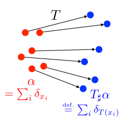
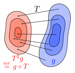
The push-forward Tsubscript𝑇T_{\sharp} of measures should not be confused with the pull-back of functions T:𝒞(𝒴)𝒞(𝒳):superscript𝑇𝒞𝒴𝒞𝒳T^{\sharp}:\mathcal{C}(\mathcal{Y})\rightarrow\mathcal{C}(\mathcal{X}) which corresponds to “warping” between functions, defined as the linear map which to g𝒞(𝒴)𝑔𝒞𝒴g\in\mathcal{C}(\mathcal{Y}) associates Tg=gTsuperscript𝑇𝑔𝑔𝑇T^{\sharp}g=g\circ T. Push-forward and pull-back are actually adjoint to one another, in the sense that (α,g)(𝒳)×𝒞(𝒴),𝒴gd(Tα)=𝒳(Tg)dα.formulae-sequencefor-all𝛼𝑔𝒳𝒞𝒴subscript𝒴𝑔dsubscript𝑇𝛼subscript𝒳superscript𝑇𝑔differential-d𝛼\forall\,(\alpha,g)\in\mathcal{M}(\mathcal{X})\times\mathcal{C}(\mathcal{Y}),\quad\int_{\mathcal{Y}}g\mathrm{d}(T_{\sharp}\alpha)=\int_{\mathcal{X}}(T^{\sharp}g)\mathrm{d}\alpha. Note that even if (α,β)𝛼𝛽(\alpha,\beta) have densities (ρα,ρβ)subscript𝜌𝛼subscript𝜌𝛽(\rho_{\alpha},\rho_{\beta}) with respect to a fixed measure (e.g. Lebesgue on dsuperscript𝑑\mathbb{R}^{d}), Tαsubscript𝑇𝛼T_{\sharp}\alpha does not have Tρβsuperscript𝑇subscript𝜌𝛽T^{\sharp}\rho_{\beta} as density, because of the presence of the Jacobian in (2.8). This explains why OT should be used with caution to perform image registration, because it does not operate as an image warping method. Figure 2.3 illustrates the distinction between these push-forward and pull-back operators.
Refer to caption Refer to caption
Push-forward of measures Pull-back of functions
Figure 2.3: Comparison of the push-forward operator Tsubscript𝑇T_{\sharp}, which can take as an input any measure, and the pull-back operator Tsuperscript𝑇T^{\sharp}, which operates on functions, notaly densities.
Remark 2.9 (Measures and random variables).
Radon measures can also be viewed as representing the distributions of random variables. A random variable X𝑋X on 𝒳𝒳\mathcal{X} is actually a map X:Ω𝒳:𝑋Ω𝒳X:\Omega\rightarrow\mathcal{X} from some abstract (often unspecified) probability space (Ω,)Ω(\Omega,\mathbb{P}), and its distribution α𝛼\alpha is the Radon measure α+1(𝒳)𝛼superscriptsubscript1𝒳\alpha\in\mathcal{M}_{+}^{1}(\mathcal{X}) such that (XA)=α(A)=Adα(x)𝑋𝐴𝛼𝐴subscript𝐴differential-d𝛼𝑥\mathbb{P}(X\in A)=\alpha(A)=\int_{A}\mathrm{d}\alpha(x). Equivalently, it is the push-forward of \mathbb{P} by X𝑋X, α=X𝛼subscript𝑋\alpha=X_{\sharp}\mathbb{P}. Applying another push-forward β=Tα𝛽subscript𝑇𝛼\beta=T_{\sharp}\alpha for T:𝒳𝒴:𝑇𝒳𝒴T:\mathcal{X}\rightarrow\mathcal{Y}, following (2.6), is equivalent to defining another random variable Y=T(X):ωΩT(X(ω))Y:𝑌𝑇𝑋𝜔Ω𝑇𝑋𝜔𝑌Y=T(X):\omega\in\Omega\rightarrow T(X(\omega))\in Y, so that β𝛽\beta is the distribution of Y𝑌Y. Drawing a random sample y𝑦y from Y𝑌Y is thus simply achieved by computing y=T(x)𝑦𝑇𝑥y=T(x), where x𝑥x is drawn from X𝑋X.

2.3 Kantorovich Relaxation

The assignment problem, and its generalization found in the Monge problem laid out in Remark 2.4, is not always relevant to studying discrete measures, such as those found in practical problems. Indeed, because the assignment problem is formulated as a permutation problem, it can only be used to compare uniform histograms of the same size. A direct generalization to discrete measures with nonuniform weights can be carried out using Monge’s formalism of push-forward maps, but that formulation may also be degenerate in the absence of feasible solutions satisfying the mass conservation constraint (2.4) (see the end of Remark 2.4). Additionally, the assignment problem (2.5) is combinatorial, and the feasible set for the Monge problem (2.9), despite being continuously parameterized as the set consisting in all push-forward measures that satisfy the mass conservation constraint, is nonconvex. Both are therefore difficult to solve when approached in their original formulation.

The key idea of Kantorovich (1942) is to relax the deterministic nature of transportation, namely the fact that a source point xisubscript𝑥𝑖x_{i} can only be assigned to another point or location yσisubscript𝑦subscript𝜎𝑖y_{\sigma_{i}} or T(xi)𝑇subscript𝑥𝑖T(x_{i}) only. Kantorovich proposes instead that the mass at any point xisubscript𝑥𝑖x_{i} be potentially dispatched across several locations. Kantorovich moves away from the idea that mass transportation should be deterministic to consider instead a probabilistic transport, which allows what is commonly known now as mass splitting from a source toward several targets. This flexibility is encoded using, in place of a permutation σ𝜎\sigma or a map T𝑇T, a coupling matrix P+n×mPsuperscriptsubscript𝑛𝑚\mathrm{\textbf{P}}\in\mathbb{R}_{+}^{n\times m}, where Pi,jsubscriptP𝑖𝑗\mathrm{\textbf{P}}_{i,j} describes the amount of mass flowing from bin i𝑖i toward bin j𝑗j, or from the mass found at xisubscript𝑥𝑖x_{i} toward yjsubscript𝑦𝑗y_{j} in the formalism of discrete measures (2.3). Admissible couplings admit a far simpler characterization than Monge maps,

U(a,b)=def.{P+n×m:P𝟙m=aandPT𝟙n=b},superscriptdef.Uabconditional-setPsuperscriptsubscript𝑛𝑚formulae-sequencePsubscriptdouble-struck-𝟙𝑚aandsuperscriptPTsubscriptdouble-struck-𝟙𝑛b\mathrm{\textbf{U}}(\mathrm{\textbf{a}},\mathrm{\textbf{b}})\stackrel{{\scriptstyle\mbox{\tiny def.}}}{{=}}\left\{\mathrm{\textbf{P}}\in\mathbb{R}_{+}^{n\times m}\;:\;\mathrm{\textbf{P}}\mathbb{1}_{m}=\mathrm{\textbf{a}}\quad\text{and}\quad{\mathrm{\textbf{P}}}^{\mathrm{T}}\mathbb{1}_{n}=\mathrm{\textbf{b}}\right\}, (2.10)

where we used the following matrix-vector notation:

P𝟙m=(jPi,j)inandPT𝟙n=(iPi,j)jm.formulae-sequencePsubscriptdouble-struck-𝟙𝑚subscriptsubscript𝑗subscriptP𝑖𝑗𝑖superscript𝑛andsuperscriptPTsubscriptdouble-struck-𝟙𝑛subscriptsubscript𝑖subscriptP𝑖𝑗𝑗superscript𝑚\mathrm{\textbf{P}}\mathbb{1}_{m}=\left(\sum_{j}\mathrm{\textbf{P}}_{i,j}\right)_{i}\in\mathbb{R}^{n}\quad\text{and}\quad{\mathrm{\textbf{P}}}^{\mathrm{T}}\mathbb{1}_{n}=\left(\sum_{i}\mathrm{\textbf{P}}_{i,j}\right)_{j}\in\mathbb{R}^{m}.

The set of matrices U(a,b)Uab\mathrm{\textbf{U}}(\mathrm{\textbf{a}},\mathrm{\textbf{b}}) is bounded and defined by n+m𝑛𝑚n+m equality constraints, and therefore is a convex polytope (the convex hull of a finite set of matrices) (Brualdi, 2006, §8.1).

Additionally, whereas the Monge formulation (as illustrated in the right plot of Figure 2.2) was intrisically asymmetric, Kantorovich’s relaxed formulation is always symmetric, in the sense that a coupling P is in U(a,b)Uab\mathrm{\textbf{U}}(\mathrm{\textbf{a}},\mathrm{\textbf{b}}) if and only if PTsuperscriptPT{\mathrm{\textbf{P}}}^{\mathrm{T}} is in U(b,a)Uba\mathrm{\textbf{U}}(\mathrm{\textbf{b}},\mathrm{\textbf{a}}). Kantorovich’s optimal transport problem now reads

LC(a,b)=def.minPU(a,b)C,P=def.i,jCi,jPi,j.superscriptdef.subscriptLCabPUabCPsuperscriptdef.subscript𝑖𝑗subscriptC𝑖𝑗subscriptP𝑖𝑗\mathrm{L}_{\mathrm{\textbf{C}}}(\mathrm{\textbf{a}},\mathrm{\textbf{b}})\stackrel{{\scriptstyle\mbox{\tiny def.}}}{{=}}\underset{\mathrm{\textbf{P}}\in\mathrm{\textbf{U}}(\mathrm{\textbf{a}},\mathrm{\textbf{b}})}{\min}\;\langle\mathrm{\textbf{C}},\,\mathrm{\textbf{P}}\rangle\stackrel{{\scriptstyle\mbox{\tiny def.}}}{{=}}\sum_{i,j}\mathrm{\textbf{C}}_{i,j}\mathrm{\textbf{P}}_{i,j}. (2.11)

This is a linear program (see Chapter 3), and as is usually the case with such programs, its optimal solutions are not necessarily unique.

Remark 2.10 (Mines and factories).

The Kantorovich problem finds a very natural illustration in the following resource allocation problem (see also Hitchcock (1941)). Suppose that an operator runs n𝑛n warehouses and m𝑚m factories. Each warehouse contains a valuable raw material that is needed by the factories to run properly. More precisely, each warehouse is indexed with an integer i𝑖i and contains aisubscripta𝑖\mathrm{\textbf{a}}_{i} units of the raw material. These raw materials must all be moved to the factories, with a prescribed quantity bjsubscriptb𝑗\mathrm{\textbf{b}}_{j} needed at factory j𝑗j to function properly. To transfer resources from a warehouse i𝑖i to a factory j𝑗j, the operator can use a transportation company that will charge Ci,jsubscriptC𝑖𝑗\mathrm{\textbf{C}}_{i,j} to move a single unit of the resource from location i𝑖i to location j𝑗j. We assume that the transportation company has the monopoly to transport goods and applies the same linear pricing scheme to all actors of the economy: the cost of shipping a𝑎a units of the resource from i𝑖i to j𝑗j is equal to a×Ci,j𝑎subscriptC𝑖𝑗a\times\mathrm{\textbf{C}}_{i,j}.

Faced with the problem described above, the operator chooses to solve the linear program described in Equation (2.11) to obtain a transportation plan PsuperscriptP\mathrm{\textbf{P}}^{\star} that quantifies for each pair i,j𝑖𝑗i,j the amount of goods Pi,jsubscriptP𝑖𝑗\mathrm{\textbf{P}}_{i,j} that must transported from warehouse i𝑖i to factory j𝑗j. The operator pays on aggregate a total of P,CsuperscriptPC\langle\mathrm{\textbf{P}}^{\star},\,\mathrm{\textbf{C}}\rangle to the transportation company to execute that plan.

Permutation matrices as couplings.

For a permutation σPerm(n)𝜎Perm𝑛\sigma\in\mathrm{Perm}(n), we write PσsubscriptP𝜎\mathrm{\textbf{P}}_{\sigma} for the corresponding permutation matrix,

(i,j)n2,(Pσ)i,j={1/nifj=σi,0otherwise.\forall\,(i,j)\in\llbracket n\rrbracket^{2},\quad(\mathrm{\textbf{P}}_{\sigma})_{i,j}=\left\{\begin{array}[]{l}1/n\quad\text{if}\quad j=\sigma_{i},\\ 0\quad\text{otherwise.}\end{array}\right. (2.12)

One can check that in that case

C,Pσ=1ni=1nCi,σi,CsubscriptP𝜎1𝑛superscriptsubscript𝑖1𝑛subscriptC𝑖subscript𝜎𝑖\langle\mathrm{\textbf{C}},\,\mathrm{\textbf{P}}_{\sigma}\rangle=\frac{1}{n}\sum_{i=1}^{n}\mathrm{\textbf{C}}_{i,\sigma_{i}},

which shows that the assignment problem (2.2) can be recast as a Kantorovich problem (2.11) where the couplings P are restricted to be exactly permutation matrices:

minσPerm(n)1ni=1nCi,σ(i)=minσPerm(n)C,Pσ.𝜎Perm𝑛1𝑛superscriptsubscript𝑖1𝑛subscriptC𝑖𝜎𝑖𝜎Perm𝑛CsubscriptP𝜎\underset{\sigma\in\mathrm{Perm}(n)}{\min}\;\frac{1}{n}\sum_{i=1}^{n}\mathrm{\textbf{C}}_{i,\sigma(i)}=\underset{\sigma\in\mathrm{Perm}(n)}{\min}\;\langle\mathrm{\textbf{C}},\,\mathrm{\textbf{P}}_{\sigma}\rangle.

Next, one can easily check that the set of permutation matrices is strictly included in the Birkhoff polytope U(𝟙n/n,𝟙n/n)Usubscriptdouble-struck-𝟙𝑛𝑛subscriptdouble-struck-𝟙𝑛𝑛\mathrm{\textbf{U}}(\mathbb{1}_{n}/n,\mathbb{1}_{n}/n). Indeed, for any permutation σ𝜎\sigma we have Pσ𝟙=𝟙nsubscriptP𝜎double-struck-𝟙subscriptdouble-struck-𝟙𝑛\mathrm{\textbf{P}}_{\sigma}\mathbb{1}=\mathbb{1}_{n} and PσT𝟙=𝟙nsuperscriptsubscriptP𝜎Tdouble-struck-𝟙subscriptdouble-struck-𝟙𝑛{\mathrm{\textbf{P}}_{\sigma}}^{\mathrm{T}}\mathbb{1}=\mathbb{1}_{n}, whereas 𝟙n𝟙nT/n2subscriptdouble-struck-𝟙𝑛superscriptsubscriptdouble-struck-𝟙𝑛Tsuperscript𝑛2\mathbb{1}_{n}{\mathbb{1}_{n}}^{\mathrm{T}}/n^{2} is a valid coupling but not a permutation matrix. Therefore, the minimum of C,PCP\langle\mathrm{\textbf{C}},\,\mathrm{\textbf{P}}\rangle is necessarily smaller when considering all transportation than when considering only permutation matrices:

LC(𝟙n/n,𝟙n/n)minσPerm(n)C,Pσ.subscriptLCsubscriptdouble-struck-𝟙𝑛𝑛subscriptdouble-struck-𝟙𝑛𝑛𝜎Perm𝑛CsubscriptP𝜎\mathrm{L}_{\mathrm{\textbf{C}}}(\mathbb{1}_{n}/n,\mathbb{1}_{n}/n)\leq\underset{\sigma\in\mathrm{Perm}(n)}{\min}\;\langle\mathrm{\textbf{C}},\,\mathrm{\textbf{P}}_{\sigma}\rangle.

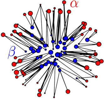
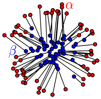
The following proposition shows that these problems result in fact in the same optimum, namely that one can always find a permutation matrix that minimizes Kantorovich’s problem (2.11) between two uniform measures a=b=𝟙n/nabsubscriptdouble-struck-𝟙𝑛𝑛\mathrm{\textbf{a}}=\mathrm{\textbf{b}}=\mathbb{1}_{n}/n. The Kantorovich relaxation is therefore tight when considered on assignment problems. Figure 2.4 shows on the left a 2-D example of optimal matching corresponding to this special case.

Proposition 2.1 (Kantorovich for matching).

If m=n𝑚𝑛m=n and a=b=𝟙n/nabsubscriptdouble-struck-𝟙𝑛𝑛\mathrm{\textbf{a}}=\mathrm{\textbf{b}}=\mathbb{1}_{n}/n, then there exists an optimal solution for Problem (2.11) PσsubscriptPsuperscript𝜎\mathrm{\textbf{P}}_{\sigma^{\star}}, which is a permutation matrix associated to an optimal permutation σPerm(n)superscript𝜎Perm𝑛\sigma^{\star}\in\mathrm{Perm}(n) for Problem (2.2).

Proof.

Birkhoff’s theorem (1946) states that the set of extremal points of U(𝟙n/n,𝟙n/n)Usubscriptdouble-struck-𝟙𝑛𝑛subscriptdouble-struck-𝟙𝑛𝑛\mathrm{\textbf{U}}(\mathbb{1}_{n}/n,\mathbb{1}_{n}/n) is equal to the set of permutation matrices. A fundamental theorem of linear programming (Bertsimas and Tsitsiklis, 1997, Theorem 2.7) states that the minimum of a linear objective in a nonempty polyhedron, if finite, is reached at an extremal point of the polyhedron. ∎
Refer to caption Refer to caption
Figure 2.4: Comparison of optimal matching and generic couplings. A black segment between xisubscript𝑥𝑖x_{i} and yjsubscript𝑦𝑗y_{j} indicates a nonzero element in the displayed optimal coupling Pi,jsubscriptP𝑖𝑗\mathrm{\textbf{P}}_{i,j} solving (2.11). Left: optimal matching, corresponding to the setting of Proposition 2.1 (empirical measures with the same number n=m𝑛𝑚n=m of points). Right: these two weighted point clouds cannot be matched; instead a Kantorovich coupling can be used to associate two arbitrary discrete measures.
Remark 2.11 (Kantorovich problem between discrete measures).
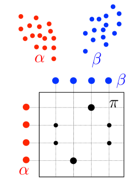
For discrete measures α,β𝛼𝛽\alpha,\beta of the form (2.3), we store in the matrix C all pairwise costs between points in the supports of α,β𝛼𝛽\alpha,\beta, namely Ci,j=def.c(xi,yj)superscriptdef.subscriptC𝑖𝑗𝑐subscript𝑥𝑖subscript𝑦𝑗\mathrm{\textbf{C}}_{i,j}\stackrel{{\scriptstyle\mbox{\tiny def.}}}{{=}}c(x_{i},y_{j}), to define c(α,β)=def.LC(a,b).superscriptdef.subscript𝑐𝛼𝛽subscriptLCab\mathcal{L}_{c}(\alpha,\beta)\stackrel{{\scriptstyle\mbox{\tiny def.}}}{{=}}\mathrm{L}_{\mathrm{\textbf{C}}}(\mathrm{\textbf{a}},\mathrm{\textbf{b}}). (2.13) Therefore, the Kantorovich formulation of optimal transport between discrete measures is the same as the problem between their associated probability weight vectors a,bab\mathrm{\textbf{a}},\mathrm{\textbf{b}} except that the cost matrix C depends on the support of α𝛼\alpha and β𝛽\beta. The notation c(α,β)subscript𝑐𝛼𝛽\mathcal{L}_{c}(\alpha,\beta), however, is useful in some situations, because it makes explicit the dependency with respect to both probability weights and supporting points, the latter being exclusively considered through the cost function c𝑐c.
Refer to caption Refer to caption Refer to caption
Discrete Semidiscrete Continuous
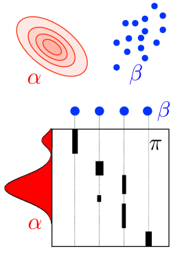
Figure 2.5: Schematic viewed of input measures (α,β)𝛼𝛽(\alpha,\beta) and couplings 𝒰(α,β)𝒰𝛼𝛽\mathcal{U}(\alpha,\beta) encountered in the three main scenarios for Kantorovich OT. Chapter 5 is dedicated to the semidiscrete setup.
Remark 2.12 (Using optimal assignments and couplings).
The optimal transport plan itself (either as a coupling P or a Monge map T𝑇T when it exists) has found many applications in data sciences, and in particular image processing. It has, for instance, been used for contrast equalization (Delon, 2004) and texture synthesis Gutierrez et al. (2017). A significant part of applications of OT to imaging sciences is for image matching (Zhu et al., 2007; Wang et al., 2013; Museyko et al., 2009; Li et al., 2013), image fusion (Courty et al., 2016), medical imaging (Wang et al., 2011) and shape registration (Makihara and Yagi, 2010; Lai and Zhao, 2017; Su et al., 2015), and image watermarking (Mathon et al., 2014). In astrophysics, OT has been used for reconstructing the early universe (Frisch et al., 2002). OT has also been used for music transcription (Flamary et al., 2016), and finds numerous applications in economics to interpret matching data (Galichon, 2016). Lastly, let us note that the computation of transportation maps computed using OT techniques (or inspired from them) is also useful to perform sampling (Reich, 2013; Oliver, 2014) and Bayesian inference (Kim et al., 2013; El Moselhy and Marzouk, 2012).
Remark 2.13 (Kantorovich problem between arbitrary measures).
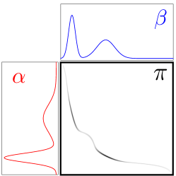
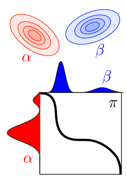
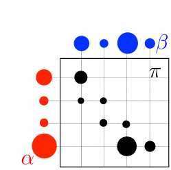
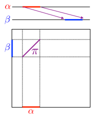
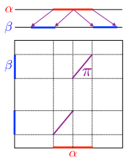
Definition (2.13) of csubscript𝑐\mathcal{L}_{c} is extended to arbitrary measures by considering couplings π+1(𝒳×𝒴)𝜋superscriptsubscript1𝒳𝒴\pi\in\mathcal{M}_{+}^{1}(\mathcal{X}\times\mathcal{Y}) which are joint distributions over the product space. The discrete case is a special situation where one imposes this product measure to be of the form π=i,jPi,jδ(xi,yj)𝜋subscript𝑖𝑗subscriptP𝑖𝑗subscript𝛿subscript𝑥𝑖subscript𝑦𝑗\pi=\sum_{i,j}\mathrm{\textbf{P}}_{i,j}\delta_{(x_{i},y_{j})}. In the general case, the mass conservation constraint (2.10) should be rewritten as a marginal constraint on joint probability distributions 𝒰(α,β)=def.{π+1(𝒳×𝒴):P𝒳π=αandP𝒴π=β}.superscriptdef.𝒰𝛼𝛽conditional-set𝜋superscriptsubscript1𝒳𝒴formulae-sequencesubscript𝑃𝒳𝜋𝛼andsubscript𝑃𝒴𝜋𝛽\mathcal{U}(\alpha,\beta)\stackrel{{\scriptstyle\mbox{\tiny def.}}}{{=}}\left\{\pi\in\mathcal{M}_{+}^{1}(\mathcal{X}\times\mathcal{Y})\;:\;P_{\mathcal{X}\sharp}\pi=\alpha\quad\text{and}\quad P_{\mathcal{Y}\sharp}\pi=\beta\right\}. (2.14) Here P𝒳subscript𝑃𝒳P_{\mathcal{X}\sharp} and P𝒴subscript𝑃𝒴P_{\mathcal{Y}\sharp} are the push-forwards (see Definition 2.1) of the projections P𝒳(x,y)=xsubscript𝑃𝒳𝑥𝑦𝑥P_{\mathcal{X}}(x,y)=x and P𝒴(x,y)=ysubscript𝑃𝒴𝑥𝑦𝑦P_{\mathcal{Y}}(x,y)=y. Figure 2.5 shows how these coupling constraints translate for different classes of problems (discrete measures and densities). Using (2.7), these marginal constraints are equivalent to imposing that π(A×𝒴)=α(A)𝜋𝐴𝒴𝛼𝐴\pi(A\times\mathcal{Y})=\alpha(A) and π(𝒳×B)=β(B)𝜋𝒳𝐵𝛽𝐵\pi(\mathcal{X}\times B)=\beta(B) for sets A𝒳𝐴𝒳A\subset\mathcal{X} and B𝒴𝐵𝒴B\subset\mathcal{Y}. The Kantorovich problem (2.11) is then generalized as c(α,β)=def.minπ𝒰(α,β)𝒳×𝒴c(x,y)dπ(x,y).superscriptdef.subscript𝑐𝛼𝛽𝜋𝒰𝛼𝛽subscript𝒳𝒴𝑐𝑥𝑦differential-d𝜋𝑥𝑦\mathcal{L}_{c}(\alpha,\beta)\stackrel{{\scriptstyle\mbox{\tiny def.}}}{{=}}\underset{\pi\in\mathcal{U}(\alpha,\beta)}{\min}\;\int_{\mathcal{X}\times\mathcal{Y}}c(x,y)\mathrm{d}\pi(x,y). (2.15) This is an infinite-dimensional linear program over a space of measures. If (𝒳,𝒴)𝒳𝒴(\mathcal{X},\mathcal{Y}) are compact spaces and c𝑐c is continuous, then it is easy to show that it always has solutions. Indeed 𝒰(α,β)𝒰𝛼𝛽\mathcal{U}(\alpha,\beta) is compact for the weak topology of measures (see Remark 2.2), πcdπmaps-to𝜋𝑐differential-d𝜋\pi\mapsto\int c\mathrm{d}\pi is a continuous function for this topology and the constraint set is nonempty (for instance, αβ𝒰(α,β)tensor-product𝛼𝛽𝒰𝛼𝛽\alpha\otimes\beta\in\mathcal{U}(\alpha,\beta)). Figure 2.6 shows examples of discrete and continuous optimal coupling solving (2.15). Figure 2.7 shows other examples of optimal 1-D couplings, involving discrete and continuous marginals.
Refer to caption Refer to caption
Figure 2.6: Left: “continuous” coupling π𝜋\pi solving (2.14) between two 1-D measures with density. The coupling is localized along the graph of the Monge map (x,T(x))𝑥𝑇𝑥(x,T(x)) (displayed in black). Right: “discrete” coupling T𝑇T solving (2.11) between two discrete measures of the form (2.3). The positive entries Ti,jsubscript𝑇𝑖𝑗T_{i,j} are displayed as black disks at position (i,j)𝑖𝑗(i,j) with radius proportional to Ti,jsubscript𝑇𝑖𝑗T_{i,j}.
Refer to caption Refer to caption Refer to caption Refer to caption
Figure 2.7: Four simple examples of optimal couplings between 1-D distributions, represented as maps above (arrows) and couplings below. Inspired by Lévy and Schwindt (2018).
Remark 2.14 (Probabilistic interpretation).
Kantorovich’s problem can be reinterpreted through the prism of random variables, following Remark 2.9. Indeed, Problem (2.15) is equivalent to c(α,β)=min(X,Y){𝔼(X,Y)(c(X,Y)):Xα,Yβ},subscript𝑐𝛼𝛽𝑋𝑌conditional-setsubscript𝔼𝑋𝑌𝑐𝑋𝑌formulae-sequencesimilar-to𝑋𝛼similar-to𝑌𝛽\mathcal{L}_{c}(\alpha,\beta)=\underset{(X,Y)}{\min}\;\left\{\mathbb{E}_{(X,Y)}(c(X,Y))\;:\;X\sim\alpha,Y\sim\beta\right\}, (2.16) where (X,Y)𝑋𝑌(X,Y) is a couple of random variables over 𝒳×𝒴𝒳𝒴\mathcal{X}\times\mathcal{Y} and Xαsimilar-to𝑋𝛼X\sim\alpha (resp., Yβsimilar-to𝑌𝛽Y\sim\beta) means that the law of X𝑋X (resp., Y𝑌Y), represented as a measure, must be α𝛼\alpha (resp., β𝛽\beta). The law of the couple (X,Y)𝑋𝑌(X,Y) is then π𝒰(α,β)𝜋𝒰𝛼𝛽\pi\in\mathcal{U}(\alpha,\beta) over the product space 𝒳×𝒴𝒳𝒴\mathcal{X}\times\mathcal{Y}.

2.4 Metric Properties of Optimal Transport

An important feature of OT is that it defines a distance between histograms and probability measures as soon as the cost matrix satisfies certain suitable properties. Indeed, OT can be understood as a canonical way to lift a ground distance between points to a distance between histogram or measures.

We first consider the case where, using a term first introduced by Rubner et al. (2000), the “ground metric” matrix C is fixed, representing substitution costs between bins, and shared across several histograms we would like to compare. The following proposition states that OT provides a valid distance between histograms supported on these bins.

Proposition 2.2.

We suppose n=m𝑛𝑚n=m and that for some p1𝑝1p\geq 1, C=Dp=(Di,jp)i,jn×nCsuperscriptD𝑝subscriptsuperscriptsubscriptD𝑖𝑗𝑝𝑖𝑗superscript𝑛𝑛\mathrm{\textbf{C}}=\mathrm{\textbf{D}}^{p}=(\mathrm{\textbf{D}}_{i,j}^{p})_{i,j}\in\mathbb{R}^{n\times n}, where D+n×nDsuperscriptsubscript𝑛𝑛\mathrm{\textbf{D}}\in\mathbb{R}_{+}^{n\times n} is a distance on ndelimited-⟦⟧𝑛\llbracket n\rrbracket, i.e.

  1. (i)

    D+n×nDsuperscriptsubscript𝑛𝑛\mathrm{\textbf{D}}\in\mathbb{R}_{+}^{n\times n} is symmetric;

  2. (ii)

    Di,j=0subscriptD𝑖𝑗0\mathrm{\textbf{D}}_{i,j}=0 if and only if i=j𝑖𝑗i=j;

  3. (iii)

    (i,j,k)n3,Di,kDi,j+Dj,k\forall\,(i,j,k)\in\llbracket n\rrbracket^{3},\mathrm{\textbf{D}}_{i,k}\leq\mathrm{\textbf{D}}_{i,j}+\mathrm{\textbf{D}}_{j,k}.

Then

Wp(a,b)=def.LDp(a,b)1/psuperscriptdef.subscriptW𝑝absubscriptLsuperscriptD𝑝superscriptab1𝑝\operatorname{\mathrm{W}}_{p}(\mathrm{\textbf{a}},\mathrm{\textbf{b}})\stackrel{{\scriptstyle\mbox{\tiny def.}}}{{=}}\mathrm{L}_{\mathrm{\textbf{D}}^{p}}(\mathrm{\textbf{a}},\mathrm{\textbf{b}})^{1/p} (2.17)

(note that WpsubscriptW𝑝\operatorname{\mathrm{W}}_{p} depends on D) defines the p𝑝p-Wasserstein distance on ΣnsubscriptΣ𝑛\Sigma_{n}, i.e. WpsubscriptW𝑝\operatorname{\mathrm{W}}_{p} is symmetric, positive, Wp(a,b)=0subscriptW𝑝ab0\operatorname{\mathrm{W}}_{p}(\mathrm{\textbf{a}},\mathrm{\textbf{b}})=0 if and only if a=bab\mathrm{\textbf{a}}=\mathrm{\textbf{b}}, and it satisfies the triangle inequality

a,b,cΣn,Wp(a,c)Wp(a,b)+Wp(b,c).formulae-sequencefor-allabcsubscriptΣ𝑛subscriptW𝑝acsubscriptW𝑝absubscriptW𝑝bc\forall\,\mathrm{\textbf{a}},\mathrm{\textbf{b}},\mathrm{\textbf{c}}\in\Sigma_{n},\quad\operatorname{\mathrm{W}}_{p}(\mathrm{\textbf{a}},\mathrm{\textbf{c}})\leq\operatorname{\mathrm{W}}_{p}(\mathrm{\textbf{a}},\mathrm{\textbf{b}})+\operatorname{\mathrm{W}}_{p}(\mathrm{\textbf{b}},\mathrm{\textbf{c}}).
Proof.

Symmetry and definiteness of the distance are easy to prove: since C=DpCsuperscriptD𝑝\mathrm{\textbf{C}}=\mathrm{\textbf{D}}^{p} has a null diagonal, Wp(a,a)=0subscriptW𝑝aa0\operatorname{\mathrm{W}}_{p}(\mathrm{\textbf{a}},\mathrm{\textbf{a}})=0, with corresponding optimal transport matrix P=diag(a)superscriptPdiaga\mathrm{\textbf{P}}^{\star}=\operatorname{diag}(\mathrm{\textbf{a}}); by the positivity of all off-diagonal elements of DpsuperscriptD𝑝\mathrm{\textbf{D}}^{p}, Wp(a,b)>0subscriptW𝑝ab0\operatorname{\mathrm{W}}_{p}(\mathrm{\textbf{a}},\mathrm{\textbf{b}})>0 whenever abab\mathrm{\textbf{a}}\neq\mathrm{\textbf{b}} (because in this case, an admissible coupling necessarily has a nonzero element outside the diagonal); by symmetry of DpsuperscriptD𝑝\mathrm{\textbf{D}}^{p}, Wp(a,b)subscriptW𝑝ab\operatorname{\mathrm{W}}_{p}(\mathrm{\textbf{a}},\mathrm{\textbf{b}}) is itself a symmetric function.

To prove the triangle inequality of Wasserstein distances for arbitrary measures, Villani (2003, Theorem 7.3) uses the gluing lemma, which stresses the existence of couplings with a prescribed structure. In the discrete setting, the explicit constuction of this glued coupling is simple. Let a,b,cΣnabcsubscriptΣ𝑛\mathrm{\textbf{a}},\mathrm{\textbf{b}},\mathrm{\textbf{c}}\in\Sigma_{n}. Let P and Q be two optimal solutions of the transport problems between a and b, and b and c, respectively. To avoid issues that may arise from null coordinates in b, we define a vector b~~b\tilde{\mathrm{\textbf{b}}} such that b~j=def.bjsuperscriptdef.subscript~b𝑗subscriptb𝑗\tilde{\mathrm{\textbf{b}}}_{j}\stackrel{{\scriptstyle\mbox{\tiny def.}}}{{=}}\mathrm{\textbf{b}}_{j} if bj>0subscriptb𝑗0\mathrm{\textbf{b}}_{j}>0, and b~j=def.1superscriptdef.subscript~b𝑗1\tilde{\mathrm{\textbf{b}}}_{j}\stackrel{{\scriptstyle\mbox{\tiny def.}}}{{=}}1 otherwise, to write

SS=def.Pdiag(1/b~)Q+n×n,superscriptdef.SSPdiag1~bQsuperscriptsubscript𝑛𝑛\SS\stackrel{{\scriptstyle\mbox{\tiny def.}}}{{=}}\mathrm{\textbf{P}}\operatorname{diag}(1/\tilde{\mathrm{\textbf{b}}})\mathrm{\textbf{Q}}\in\mathbb{R}_{+}^{n\times n},

and notice that SSU(a,c)SSUac\SS\in\mathrm{\textbf{U}}(\mathrm{\textbf{a}},\mathrm{\textbf{c}}) because

SS𝟙n=Pdiag(1/b~)Q𝟙n=P(b/b~)=P𝟙Supp(b)=a,SSsubscriptdouble-struck-𝟙𝑛Pdiag1~bQsubscriptdouble-struck-𝟙𝑛Pb~bPsubscriptdouble-struck-𝟙Suppba\SS\mathbb{1}_{n}=\mathrm{\textbf{P}}\operatorname{diag}(1/\tilde{\mathrm{\textbf{b}}})\mathrm{\textbf{Q}}\mathbb{1}_{n}=\mathrm{\textbf{P}}(\mathrm{\textbf{b}}/\tilde{\mathrm{\textbf{b}}})=\mathrm{\textbf{P}}\mathbb{1}_{\operatorname{Supp}(\mathrm{\textbf{b}})}=\mathrm{\textbf{a}},

where we denoted 𝟙Supp(b)subscriptdouble-struck-𝟙Suppb\mathbb{1}_{\operatorname{Supp}(\mathrm{\textbf{b}})} the vector of size n𝑛n with ones located at those indices j𝑗j where bj>0subscriptb𝑗0\mathrm{\textbf{b}}_{j}>0 and zero otherwise, and we use the fact that P𝟙Supp(b)=P𝟙=aPsubscriptdouble-struck-𝟙SuppbPdouble-struck-𝟙a\mathrm{\textbf{P}}\mathbb{1}_{\operatorname{Supp}(\mathrm{\textbf{b}})}=\mathrm{\textbf{P}}\mathbb{1}=\mathrm{\textbf{a}} because necessarily Pi,j=0subscriptP𝑖𝑗0\mathrm{\textbf{P}}_{i,j}=0 for those j𝑗j where bj=0subscriptb𝑗0\mathrm{\textbf{b}}_{j}=0. Similarly one verifies that SST𝟙n=csuperscriptSSTsubscriptdouble-struck-𝟙𝑛c{\SS}^{\mathrm{T}}\mathbb{1}_{n}=\mathrm{\textbf{c}}. The triangle inequality follows then from

Wp(a,c)subscriptW𝑝ac\displaystyle\operatorname{\mathrm{W}}_{p}(\mathrm{\textbf{a}},\mathrm{\textbf{c}}) =(minPU(a,c)P,Dp)1/pSS,Dp1/pabsentsuperscriptsubscriptP𝑈acPsuperscriptD𝑝1𝑝superscriptSSsuperscriptD𝑝1𝑝\displaystyle=\left(\min_{\mathrm{\textbf{P}}\in U(\mathrm{\textbf{a}},\mathrm{\textbf{c}})}\langle\mathrm{\textbf{P}},\,\mathrm{\textbf{D}}^{p}\rangle\right)^{1/p}\leq\langle\SS,\,\mathrm{\textbf{D}}^{p}\rangle^{1/p}
=(ikDikpjPijQjkb~j)1/p(ijk(Dij+Djk)pPijQjkb~j)1/pabsentsuperscriptsubscript𝑖𝑘subscriptsuperscriptD𝑝𝑖𝑘subscript𝑗subscriptP𝑖𝑗subscriptQ𝑗𝑘subscript~b𝑗1𝑝superscriptsubscript𝑖𝑗𝑘superscriptsubscriptD𝑖𝑗subscriptD𝑗𝑘𝑝subscriptP𝑖𝑗subscriptQ𝑗𝑘subscript~b𝑗1𝑝\displaystyle=\left(\sum_{ik}\mathrm{\textbf{D}}^{p}_{ik}\sum_{j}\frac{\mathrm{\textbf{P}}_{ij}\mathrm{\textbf{Q}}_{jk}}{\tilde{\mathrm{\textbf{b}}}_{j}}\right)^{1/p}\leq\left(\sum_{ijk}\left(\mathrm{\textbf{D}}_{ij}+\mathrm{\textbf{D}}_{jk}\right)^{p}\frac{\mathrm{\textbf{P}}_{ij}\mathrm{\textbf{Q}}_{jk}}{\tilde{\mathrm{\textbf{b}}}_{j}}\right)^{1/p}
(ijkDijpPijQjkb~j)1/p+(ijkDjkpPijQjkb~j)1/p.absentsuperscriptsubscript𝑖𝑗𝑘subscriptsuperscriptD𝑝𝑖𝑗subscriptP𝑖𝑗subscriptQ𝑗𝑘subscript~b𝑗1𝑝superscriptsubscript𝑖𝑗𝑘subscriptsuperscriptD𝑝𝑗𝑘subscriptP𝑖𝑗subscriptQ𝑗𝑘subscript~b𝑗1𝑝\displaystyle\leq\left(\sum_{ijk}\mathrm{\textbf{D}}^{p}_{ij}\frac{\mathrm{\textbf{P}}_{ij}\mathrm{\textbf{Q}}_{jk}}{\tilde{\mathrm{\textbf{b}}}_{j}}\right)^{1/p}+\left(\sum_{ijk}\mathrm{\textbf{D}}^{p}_{jk}\frac{\mathrm{\textbf{P}}_{ij}\mathrm{\textbf{Q}}_{jk}}{\tilde{\mathrm{\textbf{b}}}_{j}}\right)^{1/p}.

The first inequality is due to the suboptimality of SSSS\SS, the second is the triangle inequality for elements in D, and the third comes from Minkowski’s inequality. One thus has

Wp(a,c)subscriptW𝑝ac\displaystyle\operatorname{\mathrm{W}}_{p}(\mathrm{\textbf{a}},\mathrm{\textbf{c}}) (ijDijpPijkQjkb~j)1/p+(jkDjkpQjkiPijb~j)1/pabsentsuperscriptsubscript𝑖𝑗subscriptsuperscriptD𝑝𝑖𝑗subscriptP𝑖𝑗subscript𝑘subscriptQ𝑗𝑘subscript~b𝑗1𝑝superscriptsubscript𝑗𝑘subscriptsuperscriptD𝑝𝑗𝑘subscriptQ𝑗𝑘subscript𝑖subscriptP𝑖𝑗subscript~b𝑗1𝑝\displaystyle\leq\left(\sum_{ij}\mathrm{\textbf{D}}^{p}_{ij}\mathrm{\textbf{P}}_{ij}\sum_{k}\frac{\mathrm{\textbf{Q}}_{jk}}{\tilde{\mathrm{\textbf{b}}}_{j}}\right)^{1/p}+\left(\sum_{jk}\mathrm{\textbf{D}}^{p}_{jk}\mathrm{\textbf{Q}}_{jk}\sum_{i}\frac{\mathrm{\textbf{P}}_{ij}}{\tilde{\mathrm{\textbf{b}}}_{j}}\right)^{1/p}
=(ijDijpPij)1/p+(jkDjkpQjk)1/pabsentsuperscriptsubscript𝑖𝑗subscriptsuperscriptD𝑝𝑖𝑗subscriptP𝑖𝑗1𝑝superscriptsubscript𝑗𝑘subscriptsuperscriptD𝑝𝑗𝑘subscriptQ𝑗𝑘1𝑝\displaystyle=\left(\sum_{ij}\mathrm{\textbf{D}}^{p}_{ij}\mathrm{\textbf{P}}_{ij}\right)^{1/p}+\left(\sum_{jk}\mathrm{\textbf{D}}^{p}_{jk}\mathrm{\textbf{Q}}_{jk}\right)^{1/p}
=Wp(a,b)+Wp(b,c),absentsubscriptW𝑝absubscriptW𝑝b𝑐\displaystyle=\operatorname{\mathrm{W}}_{p}(\mathrm{\textbf{a}},\mathrm{\textbf{b}})+\operatorname{\mathrm{W}}_{p}(\mathrm{\textbf{b}},c),

which concludes the proof. ∎

Remark 2.15 (The cases 0<p10𝑝10<p\leq 1).

Note that if 0<p10𝑝10<p\leq 1, then DpsuperscriptD𝑝\mathrm{\textbf{D}}^{p} is itself distance. This implies that while for p1𝑝1p\geq 1, Wp(a,b)subscriptW𝑝ab\operatorname{\mathrm{W}}_{p}(\mathrm{\textbf{a}},\mathrm{\textbf{b}}) is a distance, in the case p1𝑝1p\leq 1, it is actually Wp(a,b)p\operatorname{\mathrm{W}}_{p}(\mathrm{\textbf{a}},\mathrm{\textbf{b}})^{p} which defines a distance on the simplex.

Remark 2.16 (Applications of Wasserstein distances).
The fact that the OT distance automatically “lifts” a ground metric between bins to a metric between histograms on such bins makes it a method of choice for applications in computer vision and machine learning to compare histograms. In these fields, a classical approach is to “pool” local features (for instance, image descriptors) and compute a histogram of the empirical distribution of features (a so-called bag of features) to perform retrieval, clustering or classification; see, for instance, (Oliva and Torralba, 2001). Along a similar line of ideas, OT distances can be used over some lifted feature spaces to perform signal and image analysis (Thorpe et al., 2017). Applications to retrieval and clustering were initiated by the landmark paper (Rubner et al., 2000), with renewed applications following faster algorithms for threshold matrices C that fit for some applications, for example, in computer vision (Pele and Werman, 2008, 2009). More recent applications stress the use of the earth mover’s distance for bags-of-words, either to carry out dimensionality reduction (Rolet et al., 2016) and classify texts (Kusner et al., 2015; Huang et al., 2016), or to define an alternative loss to train multiclass classifiers that output bags-of-words (Frogner et al., 2015). Kolouri et al. (2017) provides a recent overview of such applications to signal processing and machine learning.
Remark 2.17 (Wasserstein distance between measures).
Proposition 2.2 can be generalized to deal with arbitrary measures that need not be discrete.
Proposition 2.3.
We assume 𝒳=𝒴𝒳𝒴\mathcal{X}=\mathcal{Y} and that for some p1𝑝1p\geq 1, c(x,y)=d(x,y)p𝑐𝑥𝑦𝑑superscript𝑥𝑦𝑝c(x,y)=d(x,y)^{p}, where d𝑑d is a distance on 𝒳𝒳\mathcal{X}, i.e. (i) d(x,y)=d(y,x)0𝑑𝑥𝑦𝑑𝑦𝑥0d(x,y)=d(y,x)\geq 0; (ii) d(x,y)=0𝑑𝑥𝑦0d(x,y)=0 if and only if x=y𝑥𝑦x=y; (iii) (x,y,z)𝒳3,d(x,z)d(x,y)+d(y,z)formulae-sequencefor-all𝑥𝑦𝑧superscript𝒳3𝑑𝑥𝑧𝑑𝑥𝑦𝑑𝑦𝑧\forall\,(x,y,z)\in\mathcal{X}^{3},d(x,z)\leq d(x,y)+d(y,z). Then the p𝑝p-Wasserstein distance on 𝒳𝒳\mathcal{X}, 𝒲p(α,β)=def.dp(α,β)1/psuperscriptdef.subscript𝒲𝑝𝛼𝛽subscriptsuperscript𝑑𝑝superscript𝛼𝛽1𝑝\operatorname{\mathcal{W}}_{p}(\alpha,\beta)\stackrel{{\scriptstyle\mbox{\tiny def.}}}{{=}}\mathcal{L}_{d^{p}}(\alpha,\beta)^{1/p} (2.18) (note that 𝒲psubscript𝒲𝑝\operatorname{\mathcal{W}}_{p} depends on d𝑑d), is indeed a distance, namely 𝒲psubscript𝒲𝑝\operatorname{\mathcal{W}}_{p} is symmetric, nonnegative, 𝒲p(α,β)=0subscript𝒲𝑝𝛼𝛽0\operatorname{\mathcal{W}}_{p}(\alpha,\beta)=0 if and only if α=β𝛼𝛽\alpha=\beta, and it satisfies the triangle inequality (α,β,γ)+1(𝒳)3,𝒲p(α,γ)𝒲p(α,β)+𝒲p(β,γ).formulae-sequencefor-all𝛼𝛽𝛾superscriptsubscript1superscript𝒳3subscript𝒲𝑝𝛼𝛾subscript𝒲𝑝𝛼𝛽subscript𝒲𝑝𝛽𝛾\forall\,(\alpha,\beta,\gamma)\in\mathcal{M}_{+}^{1}(\mathcal{X})^{3},\quad\operatorname{\mathcal{W}}_{p}(\alpha,\gamma)\leq\operatorname{\mathcal{W}}_{p}(\alpha,\beta)+\operatorname{\mathcal{W}}_{p}(\beta,\gamma).
Proof.
The proof follows the same approach as that for Proposition 2.2 and relies on the existence of a coupling between (α,γ)𝛼𝛾(\alpha,\gamma) obtained by “gluing” optimal couplings between (α,β)𝛼𝛽(\alpha,\beta) and (β,γ)𝛽𝛾(\beta,\gamma). ∎
Remark 2.18 (Geometric intuition and weak convergence).
The Wasserstein distance 𝒲psubscript𝒲𝑝\operatorname{\mathcal{W}}_{p} has many important properties, the most important being that it is a weak distance, i.e. it allows one to compare singular distributions (for instance, discrete ones) whose supports do not overlap and to quantify the spatial shift between the supports of two distributions. In particular, “classical” distances (or divergences) are not even defined between discrete distributions (the L2superscript𝐿2L^{2} norm can only be applied to continuous measures with a density with respect to a base measure, and the discrete 2superscript2\ell^{2} norm requires that positions (xi,yj)subscript𝑥𝑖subscript𝑦𝑗(x_{i},y_{j}) take values in a predetermined discrete set to work properly). In sharp contrast, one has that for any p>0𝑝0p>0, 𝒲pp(δx,δy)=d(x,y)superscriptsubscript𝒲𝑝𝑝subscript𝛿𝑥subscript𝛿𝑦𝑑𝑥𝑦\operatorname{\mathcal{W}}_{p}^{p}(\delta_{x},\delta_{y})=d(x,y). Indeed, it suffices to notice that 𝒰(δx,δy)={δx,y}𝒰subscript𝛿𝑥subscript𝛿𝑦subscript𝛿𝑥𝑦\mathcal{U}(\delta_{x},\delta_{y})=\{\delta_{x,y}\} and therefore the Kantorovich problem having only one feasible solution, 𝒲pp(δx,δy)superscriptsubscript𝒲𝑝𝑝subscript𝛿𝑥subscript𝛿𝑦\operatorname{\mathcal{W}}_{p}^{p}(\delta_{x},\delta_{y}) is necessarily (d(x,y)p)1/p=d(x,y)superscript𝑑superscript𝑥𝑦𝑝1𝑝𝑑𝑥𝑦(d(x,y)^{p})^{1/p}=d(x,y). This shows that 𝒲p(δx,δy)0subscript𝒲𝑝subscript𝛿𝑥subscript𝛿𝑦0\operatorname{\mathcal{W}}_{p}(\delta_{x},\delta_{y})\rightarrow 0 if xy𝑥𝑦x\rightarrow y. This property corresponds to the fact that 𝒲psubscript𝒲𝑝\operatorname{\mathcal{W}}_{p} is a way to quantify the weak convergence, as we now define.
Definition 2.2 (Weak convergence).
On a compact domain 𝒳𝒳\mathcal{X}, (αk)ksubscriptsubscript𝛼𝑘𝑘(\alpha_{k})_{k} converges weakly to α𝛼\alpha in +1(𝒳)superscriptsubscript1𝒳\mathcal{M}_{+}^{1}(\mathcal{X}) (denoted αkαsubscript𝛼𝑘𝛼\alpha_{k}\rightharpoonup\alpha) if and only if for any continuous function g𝒞(𝒳)𝑔𝒞𝒳g\in\mathcal{C}(\mathcal{X}), 𝒳gdαk𝒳gdαsubscript𝒳𝑔differential-dsubscript𝛼𝑘subscript𝒳𝑔differential-d𝛼\int_{\mathcal{X}}g\mathrm{d}\alpha_{k}\rightarrow\int_{\mathcal{X}}g\mathrm{d}\alpha. One needs to add additional decay conditions on g𝑔g on noncompact domains. This notion of weak convergence corresponds to the convergence in the law of random vectors.
This convergence can be shown to be equivalent to 𝒲p(αk,α)0subscript𝒲𝑝subscript𝛼𝑘𝛼0\operatorname{\mathcal{W}}_{p}(\alpha_{k},\alpha)\rightarrow 0 (Villani, 2009, Theorem 6.8) (together with a convergence of the moments up to order p𝑝p for unbounded metric spaces).
Remark 2.19 (Translations).
A nice feature of the Wasserstein distance over a Euclidean space 𝒳=d𝒳superscript𝑑\mathcal{X}=\mathbb{R}^{d} for the ground cost c(x,y)=xy2𝑐𝑥𝑦superscriptnorm𝑥𝑦2c(x,y)=\left\|x-y\right\|^{2} is that one can factor out translations; indeed, denoting Tτ:xxτ:subscript𝑇𝜏maps-to𝑥𝑥𝜏T_{\tau}:x\mapsto x-\tau the translation operator, one has 𝒲2(Tτα,Tτβ)2=𝒲2(α,β)22ττ,𝐦α𝐦β+ττ2,\operatorname{\mathcal{W}}_{2}(T_{\tau\sharp}\alpha,T_{\tau^{\prime}\sharp}\beta)^{2}=\operatorname{\mathcal{W}}_{2}(\alpha,\beta)^{2}-2\langle\tau-\tau^{\prime},\,\mathbf{m}_{\alpha}-\mathbf{m}_{\beta}\rangle+\left\|\tau-\tau^{\prime}\right\|^{2}, where 𝐦α=def.𝒳xdα(x)dsuperscriptdef.subscript𝐦𝛼subscript𝒳𝑥differential-d𝛼𝑥superscript𝑑\mathbf{m}_{\alpha}\stackrel{{\scriptstyle\mbox{\tiny def.}}}{{=}}\int_{\mathcal{X}}x\mathrm{d}\alpha(x)\in\mathbb{R}^{d} is the mean of α𝛼\alpha. In particular, this implies the nice decomposition of the distance as 𝒲2(α,β)2=𝒲2(α~,β~)2+𝐦α𝐦β2,\operatorname{\mathcal{W}}_{2}(\alpha,\beta)^{2}=\operatorname{\mathcal{W}}_{2}(\tilde{\alpha},\tilde{\beta})^{2}+\left\|\mathbf{m}_{\alpha}-\mathbf{m}_{\beta}\right\|^{2}, where (α~,β~)~𝛼~𝛽(\tilde{\alpha},\tilde{\beta}) are the “centered” zero mean measures α~=T𝐦αα~𝛼subscript𝑇subscript𝐦𝛼𝛼\tilde{\alpha}=T_{\mathbf{m}_{\alpha}\sharp}\alpha.
Remark 2.20 (The case p=+𝑝p=+\infty).
Informally, the limit of 𝒲ppsuperscriptsubscript𝒲𝑝𝑝\operatorname{\mathcal{W}}_{p}^{p} as p+𝑝p\rightarrow+\infty is 𝒲(α,β)=def.minπ𝒰(α,β)sup(x,y)Supp(π)d(x,y),superscriptdef.subscript𝒲𝛼𝛽𝜋𝒰𝛼𝛽𝑥𝑦Supp𝜋supremum𝑑𝑥𝑦\operatorname{\mathcal{W}}_{\infty}(\alpha,\beta)\stackrel{{\scriptstyle\mbox{\tiny def.}}}{{=}}\underset{\pi\in\mathcal{U}(\alpha,\beta)}{\min}\;\underset{(x,y)\in\operatorname{Supp}(\pi)}{\sup}\;d(x,y), (2.19) where the sup should be understood as the essential supremum according to the measure π𝜋\pi on 𝒳2superscript𝒳2\mathcal{X}^{2}. In contrast to the cases p<+𝑝p<+\infty, this is a nonconvex optimization problem, which is difficult to solve numerically and to study theoretically. The 𝒲subscript𝒲\operatorname{\mathcal{W}}_{\infty} distance is related to the Hausdorff distance between the supports of (α,β)𝛼𝛽(\alpha,\beta); see § 10.6.1. We refer to (Champion et al., 2008) for details.

2.5 Dual Problem

The Kantorovich problem (2.11) is a constrained convex minimization problem, and as such, it can be naturally paired with a so-called dual problem, which is a constrained concave maximization problem. The following fundamental proposition explains the relationship between the primal and dual problems.

Proposition 2.4.

The Kantorovich problem (2.11) admits the dual

LC(a,b)=max(f,g)R(C)f,a+g,b,subscriptLCabfgRCfagb\mathrm{L}_{\mathrm{\textbf{C}}}(\mathrm{\textbf{a}},\mathrm{\textbf{b}})=\underset{(\mathrm{\textbf{f}},\mathrm{\textbf{g}})\in\mathrm{\textbf{R}}(\mathrm{\textbf{C}})}{\max}\;\langle\mathrm{\textbf{f}},\,\mathrm{\textbf{a}}\rangle+\langle\mathrm{\textbf{g}},\,\mathrm{\textbf{b}}\rangle, (2.20)

where the set of admissible dual variables is

R(C)=def.{(f,g)n×m:(i,j)n×m,fgC}.\mathrm{\textbf{R}}(\mathrm{\textbf{C}})\stackrel{{\scriptstyle\mbox{\tiny def.}}}{{=}}\left\{(\mathrm{\textbf{f}},\mathrm{\textbf{g}})\in\mathbb{R}^{n}\times\mathbb{R}^{m}\;:\;\forall\,(i,j)\in\llbracket n\rrbracket\times\llbracket m\rrbracket,\mathrm{\textbf{f}}\oplus\mathrm{\textbf{g}}\leq\mathrm{\textbf{C}}\right\}. (2.21)

Such dual variables are often referred to as “Kantorovich potentials.”

Proof.

This result is a direct consequence of the more general result on the strong duality for linear programs (Bertsimas and Tsitsiklis, 1997, p. 148, Theo. 4.4). The easier part of the proof, namely, establishing that the right-hand side of Equation (2.20) is a lower bound of LC(a,b)subscriptLCab\mathrm{L}_{\mathrm{\textbf{C}}}(\mathrm{\textbf{a}},\mathrm{\textbf{b}}), is discussed in Remark 3.2 in the next section. For the sake of completeness, let us derive our result using Lagrangian duality. The Lagangian associated to (2.11) reads

minP0max(f,g)n×mC,P+aP𝟙m,f+bPT𝟙n,g.P0fgsuperscript𝑛superscript𝑚CPaPsubscriptdouble-struck-𝟙𝑚fbsuperscriptPTsubscriptdouble-struck-𝟙𝑛g\underset{\mathrm{\textbf{P}}\geq 0}{\min}\;\underset{(\mathrm{\textbf{f}},\mathrm{\textbf{g}})\in\mathbb{R}^{n}\times\mathbb{R}^{m}}{\max}\;\langle\mathrm{\textbf{C}},\,\mathrm{\textbf{P}}\rangle+\langle\mathrm{\textbf{a}}-\mathrm{\textbf{P}}\mathbb{1}_{m},\,\mathrm{\textbf{f}}\rangle+\langle\mathrm{\textbf{b}}-{\mathrm{\textbf{P}}}^{\mathrm{T}}\mathbb{1}_{n},\,\mathrm{\textbf{g}}\rangle. (2.22)

We exchange the min and the max above, which is always possible when considering linear programs (in finite dimension), to obtain

max(f,g)n×ma,f+b,g+minP0Cf𝟙mT𝟙ngT,P.fgsuperscript𝑛superscript𝑚afbgP0Cfsuperscriptsubscriptdouble-struck-𝟙𝑚Tsubscriptdouble-struck-𝟙𝑛superscriptgTP\underset{(\mathrm{\textbf{f}},\mathrm{\textbf{g}})\in\mathbb{R}^{n}\times\mathbb{R}^{m}}{\max}\;\langle\mathrm{\textbf{a}},\,\mathrm{\textbf{f}}\rangle+\langle\mathrm{\textbf{b}},\,\mathrm{\textbf{g}}\rangle+\underset{\mathrm{\textbf{P}}\geq 0}{\min}\;\langle\mathrm{\textbf{C}}-\mathrm{\textbf{f}}{\mathbb{1}_{m}}^{\mathrm{T}}-\mathbb{1}_{n}{\mathrm{\textbf{g}}}^{\mathrm{T}},\,\mathrm{\textbf{P}}\rangle.

We conclude by remarking that

minP0Q,P={0ifQ0,otherwiseP0QPcases0ifQ0otherwise\underset{\mathrm{\textbf{P}}\geq 0}{\min}\;\langle\mathrm{\textbf{Q}},\,\mathrm{\textbf{P}}\rangle=\left\{\begin{array}[]{l}0\quad\text{if}\quad\mathrm{\textbf{Q}}\geq 0,\\ -\infty\quad\text{otherwise}\end{array}\right.

so that the constraint reads Cf𝟙mT𝟙ngT=Cfg0Cfsuperscriptsubscriptdouble-struck-𝟙𝑚Tsubscriptdouble-struck-𝟙𝑛superscriptgTdirect-sumCfg0\mathrm{\textbf{C}}-\mathrm{\textbf{f}}{\mathbb{1}_{m}}^{\mathrm{T}}-\mathbb{1}_{n}{\mathrm{\textbf{g}}}^{\mathrm{T}}=\mathrm{\textbf{C}}-\mathrm{\textbf{f}}\oplus\mathrm{\textbf{g}}\geq 0. ∎

The primal-dual optimality relation for the Lagrangian (2.22) allows us to locate the support of the optimal transport plan (see also §3.3)

{(i,j)n×m:Pi,j>0}{(i,j)n×m:fi+gj=Ci,j}.\{(i,j)\in\llbracket n\rrbracket\times\llbracket m\rrbracket:\mathrm{\textbf{P}}_{i,j}>0\}\subset\left\{(i,j)\in\llbracket n\rrbracket\times\llbracket m\rrbracket\;:\;\mathrm{\textbf{f}}_{i}+\mathrm{\textbf{g}}_{j}=\mathrm{\textbf{C}}_{i,j}\right\}. (2.23)
Remark 2.21.

Following the interpretation given to the Kantorovich problem in Remark 2.10, we follow with an intuitive presentation of the dual. Recall that in that setup, an operator wishes to move at the least possible cost an overall amount of resources from warehouses to factories. The operator can do so by solving (2.11), follow the instructions set out in PsuperscriptP\mathrm{\textbf{P}}^{\star}, and pay P,CsuperscriptPC\langle\mathrm{\textbf{P}}^{\star},\,\mathrm{\textbf{C}}\rangle to the transportation company.

Outsourcing logistics. Suppose that the operator does not have the computational means to solve the linear program (2.11). He decides instead to outsource that task to a vendor. The vendor chooses a pricing scheme with the following structure: the vendor splits the logistic task into that of collecting and then delivering the goods and will apply a collection price fisubscriptf𝑖\mathrm{\textbf{f}}_{i} to collect a unit of resource at each warehouse i𝑖i (no matter where that unit is sent to) and a price gjsubscriptg𝑗\mathrm{\textbf{g}}_{j} to deliver a unit of resource to factory j𝑗j (no matter from which warehouse that unit comes from). On aggregate, since there are exactly aisubscripta𝑖\mathrm{\textbf{a}}_{i} units at warehouse i𝑖i and bjsubscriptb𝑗\mathrm{\textbf{b}}_{j} needed at factory j𝑗j, the vendor asks as a consequence of that pricing scheme a price of f,a+g,bfagb\langle\mathrm{\textbf{f}},\,\mathrm{\textbf{a}}\rangle+\langle\mathrm{\textbf{g}},\,\mathrm{\textbf{b}}\rangle to solve the operator’s logistic problem.

Setting prices. Note that the pricing system used by the vendor allows quite naturally for arbitrarily negative prices. Indeed, if the vendor applies a price vector f for warehouses and a price vector g for factories, then the total bill will not be changed by simultaneously decreasing all entries in f by an arbitrary number and increasing all entries of g by that same number, since the total amount of resources in all warehouses is equal to those that have to be delivered to the factories. In other words, the vendor can give the illusion of giving an extremely good deal to the operator by paying him to collect some of his goods, but compensate that loss by simply charging him more for delivering them. Knowing this, the vendor, wishing to charge as much as she can for that service, sets vectors f and g to be as high as possible.

Checking prices. In the absence of another competing vendor, the operator must therefore think of a quick way to check that the vendor’s prices are reasonable. A possible way to do so would be for the operator to compute the price LC(a,b)subscriptLCab\mathrm{L}_{\mathrm{\textbf{C}}}(\mathrm{\textbf{a}},\mathrm{\textbf{b}}) of the most efficient plan by solving problem (2.11) and check if the vendor’s offer is at the very least no larger than that amount. However, recall that the operator cannot afford such a lengthy computation in the first place. Luckily, there is a far more efficient way for the operator to check whether the vendor has a competitive offer. Recall that fisubscriptf𝑖\mathrm{\textbf{f}}_{i} is the price charged by the vendor for picking a unit at i𝑖i and gjsubscriptg𝑗\mathrm{\textbf{g}}_{j} to deliver one at j𝑗j. Therefore, the vendor’s pricing scheme implies that transferring one unit of the resource from i𝑖i to j𝑗j costs exactly fi+gjsubscriptf𝑖subscriptg𝑗\mathrm{\textbf{f}}_{i}+\mathrm{\textbf{g}}_{j}. Yet, the operator also knows that the cost of shipping one unit from i𝑖i to j𝑗j as priced by the transporting company is Ci,jsubscriptC𝑖𝑗\mathrm{\textbf{C}}_{i,j}. Therefore, if for any pair i,j𝑖𝑗i,j the aggregate price fi+gjsubscriptf𝑖subscriptg𝑗\mathrm{\textbf{f}}_{i}+\mathrm{\textbf{g}}_{j} is strictly larger that Ci,jsubscriptC𝑖𝑗\mathrm{\textbf{C}}_{i,j}, the vendor is charging more than the fair price charged by the transportation company for that task, and the operator should refuse the vendor’s offer.

Refer to caption
Figure 2.8: Consider in the left plot the optimal transport problem between two discrete measures α𝛼\alpha and β𝛽\beta, represented respectively by blue dots and red squares. The area of these markers is proportional to the weight at each location. That plot also displays the optimal transport PsuperscriptP\mathrm{\textbf{P}}^{\star} using a quadratic Euclidean cost. The corresponding dual (Kantorovich) potentials fsuperscriptf\mathrm{\textbf{f}}^{\star} and gsuperscriptg\mathrm{\textbf{g}}^{\star} that correspond to that configuration are also displayed on the right plot. Since there is a “price” fisuperscriptsubscriptf𝑖\mathrm{\textbf{f}}_{i}^{\star} for each point in α𝛼\alpha (and conversely for g and β𝛽\beta), the color at that point represents the obtained value using the color map on the right. These potentials can be interpreted as relative prices in the sense that they indicate the individual cost, under the best possible transport scheme, to move a mass away at each location in α𝛼\alpha, or on the contrary to send a mass toward any point in β𝛽\beta. The optimal transport cost is therefore equal to the sum of the squared lengths of all the arcs on the left weighted by their thickness or, alternatively, using the dual formulation, to the sum of the values (encoded with colors) multiplied by the area of each marker on the right plot.

Optimal prices as a dual problem. It is therefore in the interest of the operator to check that for all pairs i,j𝑖𝑗i,j the prices offered by the vendor verify fi+gjCi,jsubscriptf𝑖subscriptg𝑗subscriptC𝑖𝑗\mathrm{\textbf{f}}_{i}+\mathrm{\textbf{g}}_{j}\leq\mathrm{\textbf{C}}_{i,j}. Suppose that the operator does check that the vendor has provided price vectors that do comply with these n×m𝑛𝑚n\times m inequalities. Can he conclude that the vendor’s proposal is attractive? Doing a quick back of the hand calculation, the operator does indeed conclude that it is in his interest to accept that offer. Indeed, since any of his transportation plans P would have a cost P,C=i,jPi,jCi,jPCsubscript𝑖𝑗subscriptP𝑖𝑗subscriptC𝑖𝑗\langle\mathrm{\textbf{P}},\,\mathrm{\textbf{C}}\rangle=\sum_{i,j}\mathrm{\textbf{P}}_{i,j}\mathrm{\textbf{C}}_{i,j}, the operator can conclude by applying these n×m𝑛𝑚n\times m inequalities that for any transport plan P (including the optimal one PsuperscriptP\mathrm{\textbf{P}}^{\star}), the marginal constraints imply

i,jPi,jCi,jsubscript𝑖𝑗subscriptP𝑖𝑗subscriptC𝑖𝑗\displaystyle\sum_{i,j}\mathrm{\textbf{P}}_{i,j}\mathrm{\textbf{C}}_{i,j} i,jPi,j(fi+gj)=(ifijPi,j)+(jgjiPi,j)absentsubscript𝑖𝑗subscriptP𝑖𝑗subscriptf𝑖subscriptg𝑗subscript𝑖subscriptf𝑖subscript𝑗subscriptP𝑖𝑗subscript𝑗subscriptg𝑗subscript𝑖subscriptP𝑖𝑗\displaystyle\geq\sum_{i,j}\mathrm{\textbf{P}}_{i,j}\left(\mathrm{\textbf{f}}_{i}+\mathrm{\textbf{g}}_{j}\right)=\left(\sum_{i}\mathrm{\textbf{f}}_{i}\sum_{j}\mathrm{\textbf{P}}_{i,j}\right)+\left(\sum_{j}\mathrm{\textbf{g}}_{j}\sum_{i}\mathrm{\textbf{P}}_{i,j}\right)
=f,a+g,b,absentfagb\displaystyle=\langle\mathrm{\textbf{f}},\,\mathrm{\textbf{a}}\rangle+\langle\mathrm{\textbf{g}},\,\mathrm{\textbf{b}}\rangle,

and therefore observe that any attempt at doing the job by himself would necessarily be more expensive than the vendor’s price.

Knowing this, the vendor must therefore find a set of prices f,gfg\mathrm{\textbf{f}},\mathrm{\textbf{g}} that maximize f,a+g,bfagb\langle\mathrm{\textbf{f}},\,\mathrm{\textbf{a}}\rangle+\langle\mathrm{\textbf{g}},\,\mathrm{\textbf{b}}\rangle but that must satisfy at the very least for all i,j𝑖𝑗i,j the basic inequality that fi+gjCi,jsubscriptf𝑖subscriptg𝑗subscriptC𝑖𝑗\mathrm{\textbf{f}}_{i}+\mathrm{\textbf{g}}_{j}\leq\mathrm{\textbf{C}}_{i,j} for his offer to be accepted, which results in Problem (2.20). One can show, as we do later in §3.1, that the best price obtained by the vendor is in fact exactly equal to the best possible cost the operator would obtain by computing LC(a,b)subscriptLCab\mathrm{L}_{\mathrm{\textbf{C}}}(\mathrm{\textbf{a}},\mathrm{\textbf{b}}).

Figure 2.8 illustrates the primal and dual solutions resulting from the same transport problem. On the left, blue dots represent warehouses and red dots stand for factories; the areas of these dots stand for the probability weights a,bab\mathrm{\textbf{a}},\mathrm{\textbf{b}}, links between them represent an optimal transport, and their width is proportional to transfered amounts. Optimal prices obtained by the vendor as a result of optimizing Problem (2.20) are shown on the right. Prices have been chosen so that their mean is equal to 0. The highest relative prices come from collecting goods at an isolated warehouse on the lower left of the figure, and delivering goods at the factory located in the upper right area.

Remark 2.22 (Dual problem between arbitrary measures).
To extend this primal-dual construction to arbitrary measures, it is important to realize that measures are naturally paired in duality with continuous functions (a measure can be accessed only through integration against continuous functions). The duality is formalized in the following proposition, which boils down to Proposition 2.4 when dealing with discrete measures.
Proposition 2.5.
One has c(α,β)=sup(f,g)(c)𝒳f(x)dα(x)+𝒴g(y)dβ(y),subscript𝑐𝛼𝛽𝑓𝑔𝑐supremumsubscript𝒳𝑓𝑥differential-d𝛼𝑥subscript𝒴𝑔𝑦differential-d𝛽𝑦\mathcal{L}_{c}(\alpha,\beta)=\underset{(f,g)\in\mathcal{R}(c)}{\sup}\;\int_{\mathcal{X}}f(x)\mathrm{d}\alpha(x)+\int_{\mathcal{Y}}g(y)\mathrm{d}\beta(y), (2.24) where the set of admissible dual potentials is (c)=def.{(f,g)𝒞(𝒳)×𝒞(𝒴):(x,y),f(x)+g(y)c(x,y)}.superscriptdef.𝑐conditional-set𝑓𝑔𝒞𝒳𝒞𝒴for-all𝑥𝑦𝑓𝑥𝑔𝑦𝑐𝑥𝑦\mathcal{R}(c)\stackrel{{\scriptstyle\mbox{\tiny def.}}}{{=}}\left\{(f,g)\in\mathcal{C}(\mathcal{X})\times\mathcal{C}(\mathcal{Y})\;:\;\forall(x,y),f(x)+g(y)\leq c(x,y)\right\}. (2.25) Here, (f,g)𝑓𝑔(f,g) is a pair of continuous functions and are also called, as in the discrete case, “Kantorovich potentials.”
The discrete case (2.20) corresponds to the dual vectors being samples of the continuous potentials, i.e. (fi,gj)=(f(xi),g(yj))subscriptf𝑖subscriptg𝑗𝑓subscript𝑥𝑖𝑔subscript𝑦𝑗(\mathrm{\textbf{f}}_{i},\mathrm{\textbf{g}}_{j})=(f(x_{i}),g(y_{j})). The primal-dual optimality conditions allow us to track the support of the optimal plan, and (2.23) is generalized as Supp(π){(x,y)𝒳×𝒴:f(x)+g(y)=c(x,y)}.Supp𝜋conditional-set𝑥𝑦𝒳𝒴𝑓𝑥𝑔𝑦𝑐𝑥𝑦\operatorname{Supp}(\pi)\subset\left\{(x,y)\in\mathcal{X}\times\mathcal{Y}\;:\;f(x)+g(y)=c(x,y)\right\}. (2.26) Note that in contrast to the primal problem (2.15), showing the existence of solutions to (2.24) is nontrivial, because the constraint set (c)𝑐\mathcal{R}(c) is not compact and the function to minimize noncoercive. Using the machinery of c𝑐c-transform detailed in § 5.1, in the case c(x,y)=d(x,y)p𝑐𝑥𝑦𝑑superscript𝑥𝑦𝑝c(x,y)=d(x,y)^{p} with p1𝑝1p\geq 1, one can, however, show that optimal (f,g)𝑓𝑔(f,g) are necessarily Lipschitz regular, which enables us to replace the constraint by a compact one.
Remark 2.23 (Unconstrained dual).
In the case 𝒳dα=𝒴dβ=1subscript𝒳differential-d𝛼subscript𝒴differential-d𝛽1\int_{\mathcal{X}}\mathrm{d}\alpha=\int_{\mathcal{Y}}\mathrm{d}\beta=1, the constrained dual problem (2.24) can be replaced by an unconstrained one, c(α,β)=sup(f,g)𝒞(𝒳)×𝒞(𝒴)𝒳fdα+𝒴gdβ+min𝒳𝒴(cfg),subscript𝑐𝛼𝛽𝑓𝑔𝒞𝒳𝒞𝒴supremumsubscript𝒳𝑓differential-d𝛼subscript𝒴𝑔differential-d𝛽tensor-product𝒳𝒴direct-sum𝑐𝑓𝑔\mathcal{L}_{c}(\alpha,\beta)=\underset{(f,g)\in\mathcal{C}(\mathcal{X})\times\mathcal{C}(\mathcal{Y})}{\sup}\;\int_{\mathcal{X}}f\mathrm{d}\alpha+\int_{\mathcal{Y}}g\mathrm{d}\beta+\underset{\mathcal{X}\otimes\mathcal{Y}}{\min}\;(c-f\oplus g), (2.27) where we denoted (fg)(x,y)=f(x)+g(y)direct-sum𝑓𝑔𝑥𝑦𝑓𝑥𝑔𝑦(f\oplus g)(x,y)=f(x)+g(y). Here the minimum should be considered as the essential supremum associated to the measure αβtensor-product𝛼𝛽\alpha\otimes\beta, i.e., it does not change if f𝑓f or g𝑔g is modified on sets of zero measure for α𝛼\alpha and β𝛽\beta. This alternative dual formulation was pointed out to us by Francis Bach. It is obtained from the primal problem (2.15) by adding the redundant constraint dπ=1differential-d𝜋1\int\mathrm{d}\pi=1.
Remark 2.24 (Monge–Kantorovich equivalence—Brenier theorem).
The following theorem is often attributed to Brenier (1991) and ensures that in dsuperscript𝑑\mathbb{R}^{d} for p=2𝑝2p=2, if at least one of the two input measures has a density, and for measures with second order moments, then the Kantorovich and Monge problems are equivalent. The interested reader should also consult variants of the same result published more or less at the same time by Cuesta and Matran (1989); Rüschendorf and Rachev (1990), including notably the original result in (Brenier, 1987) and a precursor by Knott and Smith (1984).
Theorem 2.1 (Brenier).
In the case 𝒳=𝒴=d𝒳𝒴superscript𝑑\mathcal{X}=\mathcal{Y}=\mathbb{R}^{d} and c(x,y)=xy2𝑐𝑥𝑦superscriptnorm𝑥𝑦2c(x,y)=\left\|x-y\right\|^{2}, if at least one of the two input measures (denoted α𝛼\alpha) has a density ραsubscript𝜌𝛼\rho_{\alpha} with respect to the Lebesgue measure, then the optimal π𝜋\pi in the Kantorovich formulation (2.15) is unique and is supported on the graph (x,T(x))𝑥𝑇𝑥(x,T(x)) of a “Monge map” T:dd:𝑇superscript𝑑superscript𝑑T:\mathbb{R}^{d}\rightarrow\mathbb{R}^{d}. This means that π=(Id,T)α𝜋subscriptId𝑇𝛼\pi=(\mathrm{Id},T)_{\sharp}\alpha, i.e. h𝒞(𝒳×𝒴),𝒳×𝒴h(x,y)dπ(x,y)=𝒳h(x,T(x))dα(x).formulae-sequencefor-all𝒞𝒳𝒴subscript𝒳𝒴𝑥𝑦differential-d𝜋𝑥𝑦subscript𝒳𝑥𝑇𝑥differential-d𝛼𝑥\forall\,h\in\mathcal{C}(\mathcal{X}\times\mathcal{Y}),\quad\int_{\mathcal{X}\times\mathcal{Y}}h(x,y)\mathrm{d}\pi(x,y)=\int_{\mathcal{X}}h(x,T(x))\mathrm{d}\alpha(x). (2.28) Furthermore, this map T𝑇T is uniquely defined as the gradient of a convex function φ𝜑\varphi, T(x)=φ(x)𝑇𝑥𝜑𝑥T(x)=\nabla\varphi(x), where φ𝜑\varphi is the unique (up to an additive constant) convex function such that (φ)α=βsubscript𝜑𝛼𝛽(\nabla\varphi)_{\sharp}\alpha=\beta. This convex function is related to the dual potential f𝑓f solving (2.24) as φ(x)=x22f(x)𝜑𝑥superscriptnorm𝑥22𝑓𝑥\varphi(x)=\frac{\left\|x\right\|^{2}}{2}-f(x).
Proof.
We sketch the main ingredients of the proof; more details can be found, for instance, in (Santambrogio, 2015). We remark that cdπ=Cα,β2x,ydπ(x,y)𝑐differential-d𝜋subscript𝐶𝛼𝛽2𝑥𝑦differential-d𝜋𝑥𝑦\int c\mathrm{d}\pi=C_{\alpha,\beta}-2\int\langle x,\,y\rangle\mathrm{d}\pi(x,y), where the constant is Cα,β=x2dα(x)+y2dβ(y)subscript𝐶𝛼𝛽superscriptnorm𝑥2differential-d𝛼𝑥superscriptnorm𝑦2differential-d𝛽𝑦C_{\alpha,\beta}=\int\left\|x\right\|^{2}\mathrm{d}\alpha(x)+\int\left\|y\right\|^{2}\mathrm{d}\beta(y). Instead of solving (2.15), one can thus consider the problem maxπ𝒰(α,β)𝒳×𝒴x,ydπ(x,y),𝜋𝒰𝛼𝛽subscript𝒳𝒴𝑥𝑦differential-d𝜋𝑥𝑦\underset{\pi\in\mathcal{U}(\alpha,\beta)}{\max}\;\int_{\mathcal{X}\times\mathcal{Y}}\langle x,\,y\rangle\mathrm{d}\pi(x,y), whose dual reads min(φ,ψ){𝒳φdα+𝒴ψdβ:(x,y),φ(x)+ψ(y)x,y}.𝜑𝜓conditional-setsubscript𝒳𝜑differential-d𝛼subscript𝒴𝜓differential-d𝛽for-all𝑥𝑦𝜑𝑥𝜓𝑦𝑥𝑦\underset{(\varphi,\psi)}{\min}\;\left\{\int_{\mathcal{X}}\varphi\mathrm{d}\alpha+\int_{\mathcal{Y}}\psi\mathrm{d}\beta\;:\;\forall(x,y),\quad\varphi(x)+\psi(y)\geq\langle x,\,y\rangle\right\}. (2.29) The relation between these variables and those of (2.25) is (φ,ψ)=(22f,22g)(\varphi,\psi)=(\frac{\left\|\cdot\right\|^{2}}{2}-f,\frac{\left\|\cdot\right\|^{2}}{2}-g). One can replace the constraint by y,ψ(y)φ(y)=def.sup𝑥x,yφ(x).for-all𝑦𝜓𝑦superscript𝜑𝑦superscriptdef.𝑥supremum𝑥𝑦𝜑𝑥\forall\,y,\quad\psi(y)\geq\varphi^{*}(y)\stackrel{{\scriptstyle\mbox{\tiny def.}}}{{=}}\underset{x}{\sup}\;\langle x,\,y\rangle-\varphi(x). (2.30) Here φsuperscript𝜑\varphi^{*} is the Legendre transform of φ𝜑\varphi and is a convex function as a supremum of linear forms (see also (4.54)). Since the objective appearing in (2.31) is linear and the integrating measures positive, one can minimize explicitly with respect to ψ𝜓\psi and set ψ=φ𝜓superscript𝜑\psi=\varphi^{*} in order to consider the unconstrained problem min𝜑𝒳φdα+𝒴φdβ;𝜑subscript𝒳𝜑differential-d𝛼subscript𝒴superscript𝜑differential-d𝛽\underset{\varphi}{\min}\;\int_{\mathcal{X}}\varphi\mathrm{d}\alpha+\int_{\mathcal{Y}}\varphi^{*}\mathrm{d}\beta; (2.31) see also §3.2 and §5.1, where that idea is applied respectively in the discrete setting and for generic costs c(x,y)𝑐𝑥𝑦c(x,y). By iterating this argument twice, one can replace φ𝜑\varphi by φsuperscript𝜑absent\varphi^{**}, which is a convex function, and thus impose in (2.31) that φ𝜑\varphi is convex. Condition (2.26) shows that an optimal π𝜋\pi is supported on {(x,y):φ(x)+φ(y)=x,y}conditional-set𝑥𝑦𝜑𝑥superscript𝜑𝑦𝑥𝑦\left\{(x,y)\;:\;\varphi(x)+\varphi^{*}(y)=\langle x,\,y\rangle\right\}, which shows that such a y𝑦y is optimal for the minimization (2.30) of the Legendre transform, whose optimality condition reads yφ(x)𝑦𝜑𝑥y\in\partial\varphi(x). Since φ𝜑\varphi is convex, it is differentiable almost everywhere, and since α𝛼\alpha has a density, it is also differentiable α𝛼\alpha-almost everywhere. This shows that for each x𝑥x, the associated y𝑦y is uniquely defined α𝛼\alpha-almost everywhere as y=φ(x)𝑦𝜑𝑥y=\nabla\varphi(x), and it shows that necessarily π=(Id,φ)α𝜋subscriptId𝜑𝛼\pi=(\mathrm{Id},\nabla\varphi)_{\sharp}\alpha. ∎
This result shows that in the setting of 𝒲2subscript𝒲2\operatorname{\mathcal{W}}_{2} with no-singular densities, the Monge problem (2.9) and its Kantorovich relaxation (2.15) are equal (the relaxation is tight). This is the continuous counterpart of Proposition 2.1 for the assignment case (2.1), which states that the minimum of the optimal transport problem is achieved at a permutation matrix (a discrete map) when the marginals are equal and uniform. Brenier’s theorem, stating that an optimal transport map must be the gradient of a convex function, provides a useful generalization of the notion of increasing functions in dimension more than one. This is the main reason why optimal transport can be used to define quantile functions in arbitrary dimensions, which is in turn useful for applications to quantile regression problems (Carlier et al., 2016). Note also that this theorem can be extended in many directions. The condition that α𝛼\alpha has a density can be weakened to the condition that it does not give mass to “small sets” having Hausdorff dimension smaller than d1𝑑1d-1 (e.g. hypersurfaces). One can also consider costs of the form c(x,y)=h(xy)𝑐𝑥𝑦𝑥𝑦c(x,y)=h(x-y), where hh is a strictly convex function.
Remark 2.25 (Monge–Ampère equation).
For measures with densities, using (2.8), one obtains that φ𝜑\varphi is the unique (up to the addition of a constant) convex function which solves the following Monge–Ampère-type equation: det(2φ(x))ρβ(φ(x))=ρα(x)superscript2𝜑𝑥subscript𝜌𝛽𝜑𝑥subscript𝜌𝛼𝑥\det(\partial^{2}\varphi(x))\rho_{\beta}(\nabla\varphi(x))=\rho_{\alpha}(x) (2.32) where 2φ(x)d×dsuperscript2𝜑𝑥superscript𝑑𝑑\partial^{2}\varphi(x)\in\mathbb{R}^{d\times d} is the Hessian of φ𝜑\varphi. The Monge–Ampère operator det(2φ(x))superscript2𝜑𝑥\det(\partial^{2}\varphi(x)) can be understood as a nonlinear degenerate Laplacian. In the limit of small displacements, φ=Id+εψ𝜑Id𝜀𝜓\varphi=\mathrm{Id}+\varepsilon\psi, one indeed recovers the Laplacian ΔΔ\Delta as a linearization since for smooth maps det(2φ(x))=1+εΔψ(x)+o(ε).superscript2𝜑𝑥1𝜀Δ𝜓𝑥𝑜𝜀\det(\partial^{2}\varphi(x))=1+\varepsilon\Delta\psi(x)+o(\varepsilon). The convexity constraint forces det(2φ(x))0superscript2𝜑𝑥0\det(\partial^{2}\varphi(x))\geq 0 and is necessary for this equation to have a solution. There is a large body of literature on the theoretical analysis of the Monge–Ampère equation, and in particular the regularity of its solution—see, for instance, (Gutiérrez, 2016); we refer the interested read to the review paper by Caffarelli (2003). A major difficulty is that in full generality, solutions need not be smooth, and one has to resort to the machinery of Alexandrov solutions when the input measures are arbitrary (e.g. Dirac masses). Many solvers have been proposed in the simpler case of the Monge–Ampère equation det(2φ(x))=f(x)superscript2𝜑𝑥𝑓𝑥\det(\partial^{2}\varphi(x))=f(x) for a fixed right-hand-side f𝑓f; see, for instance, (Benamou et al., 2016b) and the references therein. In particular, capturing anisotropic convex functions requires special care, and usual finite differences can be inaccurate. For optimal transport, where f𝑓f actually depends on φ𝜑\nabla\varphi, the discretization of Equation (2.32), and the boundary condition result in technical challenges outlined in (Benamou et al., 2014) and the references therein. Note also that related solvers based on fixed-point iterations have been applied to image registration (Haker et al., 2004).

2.6 Special Cases

In general, computing OT distances is numerically involved. Before detailing in §§3,4, and 7 different numerical solvers, we first review special favorable cases where the resolution of the OT problem is relatively easy.

Remark 2.26 (Binary cost matrix and 1-norm).

One can easily check that when the cost matrix C is 0 on the diagonal and 111 elsewhere, namely, when C=𝟙n×n𝕀nCsubscriptdouble-struck-𝟙𝑛𝑛subscript𝕀𝑛\mathrm{\textbf{C}}=\mathbb{1}_{n\times n}-\mathbb{I}_{n}, the 1-Wasserstein distance between a and b is equal to the 1-norm of their difference, LC(a,b)=ab1subscriptLCabsubscriptnormab1\mathrm{L}_{\mathrm{\textbf{C}}}(\mathrm{\textbf{a}},\mathrm{\textbf{b}})=\left\|\mathrm{\textbf{a}}-\mathrm{\textbf{b}}\right\|_{1}.

Remark 2.27 (Kronecker cost function and total variation).
In addition to Remark 2.26 above, one can also easily check that this result extends to arbitrary measures in the case where c(x,y)𝑐𝑥𝑦c(x,y) is 00 if x=y𝑥𝑦x=y and 1 when xy𝑥𝑦x\neq y. The OT distance between two discrete measures α𝛼\alpha and β𝛽\beta is equal to their total variation distance (see also Example 8.1.5).
Remark 2.28 (1-D case—Empirical measures).
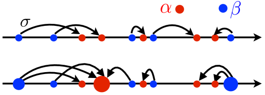
Here 𝒳=𝒳\mathcal{X}=\mathbb{R}. Assuming α=1ni=1nδxi𝛼1𝑛superscriptsubscript𝑖1𝑛subscript𝛿subscript𝑥𝑖\alpha=\frac{1}{n}\sum_{i=1}^{n}\delta_{x_{i}} and β=1nj=1nδyj𝛽1𝑛superscriptsubscript𝑗1𝑛subscript𝛿subscript𝑦𝑗\beta=\frac{1}{n}\sum_{j=1}^{n}\delta_{y_{j}}, and assuming (without loss of generality) that the points are ordered, i.e. x1x2xnsubscript𝑥1subscript𝑥2subscript𝑥𝑛x_{1}\leq x_{2}\leq\cdots\leq x_{n} and y1y2ynsubscript𝑦1subscript𝑦2subscript𝑦𝑛y_{1}\leq y_{2}\leq\cdots\leq y_{n}, then one has the simple formula 𝒲p(α,β)p=1ni=1n|xiyi|p,\operatorname{\mathcal{W}}_{p}(\alpha,\beta)^{p}=\frac{1}{n}\sum_{i=1}^{n}|x_{i}-y_{i}|^{p}, (2.33) i.e. locally (if one assumes distinct points), 𝒲p(α,β)subscript𝒲𝑝𝛼𝛽\operatorname{\mathcal{W}}_{p}(\alpha,\beta) is the psuperscript𝑝\ell^{p} norm between two vectors of ordered values of α𝛼\alpha and β𝛽\beta. That statement is valid only locally, in the sense that the order (and those vector representations) might change whenever some of the values change. That formula is a simple consequence of the more general setting detailed in Remark 2.30. Figure 2.9, top row, illustrates the 1-D transportation map between empirical measures with the same number of points. The bottom row shows how this monotone map generalizes to arbitrary discrete measures. It is also possible to leverage this 1-D computation to also compute efficiently OT on the circle as shown by Delon et al. (2010). Note that if the cost is a concave function of the distance, notably when p<1𝑝1p<1, the behavior of the optimal transport plan is very different, yet efficient solvers also exist (Delon et al., 2012).
Refer to caption
Figure 2.9: 1-D optimal couplings: each arrow xiyjsubscript𝑥𝑖subscript𝑦𝑗x_{i}\rightarrow y_{j} indicates a nonzero Pi,jsubscriptP𝑖𝑗\mathrm{\textbf{P}}_{i,j} in the optimal coupling. Top: empirical measures with same number of points (optimal matching). Bottom: generic case. This corresponds to monotone rearrangements, if xixisubscript𝑥𝑖subscript𝑥superscript𝑖x_{i}\leq x_{i^{\prime}} are such that Pi,j0,Pi,j0formulae-sequencesubscriptP𝑖𝑗0subscriptPsuperscript𝑖superscript𝑗0\mathrm{\textbf{P}}_{i,j}\neq 0,\mathrm{\textbf{P}}_{i^{\prime},j^{\prime}}\neq 0, then necessarily yjyjsubscript𝑦𝑗subscript𝑦superscript𝑗y_{j}\leq y_{j^{\prime}}.
Remark 2.29 (Histogram equalization).
One-dimensional optimal transport can be used to perform histogram equalization, with applications to the normalization of the palette of grayscale images, see Figure 2.10. In this case, one denotes (x¯i)isubscriptsubscript¯𝑥𝑖𝑖(\bar{x}_{i})_{i} and (y¯j)jsubscriptsubscript¯𝑦𝑗𝑗(\bar{y}_{j})_{j} the gray color levels (00 for black, 111 for white, and all values in between) of all pixels of the two input images enumerated in a predefined order (i.e. columnwise). Assuming the number of pixels in each image is the same and equal to n×m𝑛𝑚n\times m, sorting these color levels defines xi=x¯σ1(i)subscript𝑥𝑖subscript¯𝑥subscript𝜎1𝑖x_{i}=\bar{x}_{\sigma_{1}(i)} and yj=y¯σ2(j)subscript𝑦𝑗subscript¯𝑦subscript𝜎2𝑗y_{j}=\bar{y}_{\sigma_{2}(j)} as in Remark 2.28, where σ1,σ2:{1,,nm}{1,,nm}:subscript𝜎1subscript𝜎21𝑛𝑚1𝑛𝑚\sigma_{1},\sigma_{2}:\{1,\ldots,nm\}\rightarrow\{1,\ldots,nm\} are permutations, so that σ=def.σ2σ11superscriptdef.𝜎subscript𝜎2superscriptsubscript𝜎11\sigma\stackrel{{\scriptstyle\mbox{\tiny def.}}}{{=}}\sigma_{2}\circ\sigma_{1}^{-1} is the optimal assignment between the two discrete distributions. For image processing applications, (y¯σ(i))isubscriptsubscript¯𝑦𝜎𝑖𝑖(\bar{y}_{\sigma(i)})_{i} defines the color values of an equalized version of x¯¯𝑥\bar{x}, whose empirical distribution matches exactly the one of y¯¯𝑦\bar{y}. The equalized version of that image can be recovered by folding back that nm𝑛𝑚nm-dimensional vector as an image of size n×m𝑛𝑚n\times m. Also, t[0,1](1t)x¯i+ty¯σ(i)𝑡01maps-to1𝑡subscript¯𝑥𝑖𝑡subscript¯𝑦𝜎𝑖t\in[0,1]\mapsto(1-t)\bar{x}_{i}+t\bar{y}_{\sigma(i)} defines an interpolation between the original image and the equalized one, whose empirical distribution of pixels is the displacement interpolation (as defined in (7.7)) between those of the inputs.
Refer to caption Refer to caption Refer to caption Refer to caption Refer to caption
t=0𝑡0t=0 t=0.25𝑡0.25t=0.25 t=0.5𝑡0.5t=0.5 t=.75𝑡.75t=.75 t=1𝑡1t=1
Figure 2.10: Histogram equalization for image processing, where t𝑡t parameterizes the displacement interpolation between the histograms.
Remark 2.30 (1-D case—Generic case).
For a measure α𝛼\alpha on \mathbb{R}, we introduce the cumulative distribution function from \mathbb{R} to [0,1]absent01\rightarrow[0,1] defined as x,𝒞α(x)=def.xdα,formulae-sequencefor-all𝑥superscriptdef.subscript𝒞𝛼𝑥superscriptsubscript𝑥differential-d𝛼\forall\,x\in\mathbb{R},\quad\mathcal{C}_{\alpha}(x)\stackrel{{\scriptstyle\mbox{\tiny def.}}}{{=}}\int_{-\infty}^{x}\mathrm{d}\alpha, (2.34) and its pseudoinverse 𝒞α1:[0,1]{}:superscriptsubscript𝒞𝛼101\mathcal{C}_{\alpha}^{-1}:[0,1]\rightarrow\mathbb{R}\cup\{-\infty\} r[0,1],𝒞α1(r)=min𝑥{x{}:𝒞α(x)r}.formulae-sequencefor-all𝑟01superscriptsubscript𝒞𝛼1𝑟𝑥conditional-set𝑥subscript𝒞𝛼𝑥𝑟\forall\,r\in[0,1],\quad\mathcal{C}_{\alpha}^{-1}(r)=\underset{x}{\min}\;\left\{x\in\mathbb{R}\cup\{-\infty\}\;:\;\mathcal{C}_{\alpha}(x)\geq r\right\}. (2.35) That function is also called the generalized quantile function of α𝛼\alpha. For any p1𝑝1p\geq 1, one has 𝒲p(α,β)p=𝒞α1𝒞β1Lp([0,1])p=01|𝒞α1(r)𝒞β1(r)|pdr.\operatorname{\mathcal{W}}_{p}(\alpha,\beta)^{p}=\left\|\mathcal{C}_{\alpha}^{-1}-\mathcal{C}_{\beta}^{-1}\right\|_{L^{p}([0,1])}^{p}=\int_{0}^{1}|\mathcal{C}_{\alpha}^{-1}(r)-\mathcal{C}_{\beta}^{-1}(r)|^{p}\mathrm{d}r. (2.36) This means that through the map α𝒞α1maps-to𝛼superscriptsubscript𝒞𝛼1\alpha\mapsto\mathcal{C}_{\alpha}^{-1}, the Wasserstein distance is isometric to a linear space equipped with the Lpsuperscript𝐿𝑝L^{p} norm or, equivalently, that the Wasserstein distance for measures on the real line is a Hilbertian metric. This makes the geometry of 1-D optimal transport very simple but also very different from its geometry in higher dimensions, which is not Hilbertian as discussed in Proposition 7 and more generally in §8.3. For p=1𝑝1p=1, one even has the simpler formula 𝒲1(α,β)subscript𝒲1𝛼𝛽\displaystyle\operatorname{\mathcal{W}}_{1}(\alpha,\beta) =𝒞α𝒞βL1()=|𝒞α(x)𝒞β(x)|dxabsentsubscriptnormsubscript𝒞𝛼subscript𝒞𝛽superscript𝐿1subscriptsubscript𝒞𝛼𝑥subscript𝒞𝛽𝑥differential-d𝑥\displaystyle=\left\|\mathcal{C}_{\alpha}-\mathcal{C}_{\beta}\right\|_{L^{1}(\mathbb{R})}=\int_{\mathbb{R}}|\mathcal{C}_{\alpha}(x)-\mathcal{C}_{\beta}(x)|\mathrm{d}x (2.37) =|xd(αβ)|dx,absentsubscriptsuperscriptsubscript𝑥d𝛼𝛽differential-d𝑥\displaystyle=\int_{\mathbb{R}}\left\lvert\int_{-\infty}^{x}\mathrm{d}(\alpha-\beta)\right\rvert\mathrm{d}x, (2.38) which shows that 𝒲1subscript𝒲1\operatorname{\mathcal{W}}_{1} is a norm (see §6.2 for the generalization to arbitrary dimensions). An optimal Monge map T𝑇T such that Tα=βsubscript𝑇𝛼𝛽T_{\sharp}\alpha=\beta is then defined by T=𝒞β1𝒞α.𝑇superscriptsubscript𝒞𝛽1subscript𝒞𝛼T=\mathcal{C}_{\beta}^{-1}\circ\mathcal{C}_{\alpha}. (2.39) Figure 2.11 illustrates the computation of 1-D OT through cumulative functions. It also displays displacement interpolations, computed as detailed in (7.7); see also Remark 6. For a detailed survey of the properties of optimal transport in one dimension, we refer the reader to (Santambrogio, 2015, Chapter 2).
Refer to caption Refer to caption Refer to caption
α𝛼\alpha β𝛽\beta (tT+(1t)Id)αsubscript𝑡𝑇1𝑡Id𝛼{(tT+(1-t)\mathrm{Id})_{\sharp}\alpha}
Refer to caption Refer to caption Refer to caption Refer to caption
(𝒞α,𝒞β)subscript𝒞𝛼subscript𝒞𝛽(\mathcal{C}_{\alpha},\mathcal{C}_{\beta}) (𝒞α1,𝒞β1)superscriptsubscript𝒞𝛼1superscriptsubscript𝒞𝛽1(\mathcal{C}_{\alpha}^{-1},\mathcal{C}_{\beta}^{-1}) (T,T1)𝑇superscript𝑇1(T,T^{-1}) (1t)𝒞α1+t𝒞β11𝑡superscriptsubscript𝒞𝛼1𝑡superscriptsubscript𝒞𝛽1(1-t)\mathcal{C}_{\alpha}^{-1}+t\mathcal{C}_{\beta}^{-1}
Figure 2.11: Computation of OT and displacement interpolation between two 1-D measures, using cumulant function as detailed in (2.39).
Remark 2.31 (Distance between Gaussians).
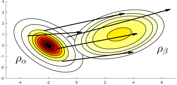
If α=𝒩(𝐦α,𝚺α)𝛼𝒩subscript𝐦𝛼subscript𝚺𝛼\alpha=\mathcal{N}(\mathbf{m}_{\alpha},\mathbf{\Sigma}_{\alpha}) and β=𝒩(𝐦β,𝚺β)𝛽𝒩subscript𝐦𝛽subscript𝚺𝛽\beta=\mathcal{N}(\mathbf{m}_{\beta},\mathbf{\Sigma}_{\beta}) are two Gaussians in dsuperscript𝑑\mathbb{R}^{d}, then one can show that the following map T:x𝐦β+A(x𝐦α),:𝑇maps-to𝑥subscript𝐦𝛽𝐴𝑥subscript𝐦𝛼T:x\mapsto\mathbf{m}_{\beta}+A(x-\mathbf{m}_{\alpha}), (2.40) where A=𝚺α12(𝚺α12𝚺β𝚺α12)12𝚺α12=AT,𝐴superscriptsubscript𝚺𝛼12superscriptsuperscriptsubscript𝚺𝛼12subscript𝚺𝛽superscriptsubscript𝚺𝛼1212superscriptsubscript𝚺𝛼12superscript𝐴TA=\mathbf{\Sigma}_{\alpha}^{-\tfrac{1}{2}}\Big{(}\mathbf{\Sigma}_{\alpha}^{\tfrac{1}{2}}\mathbf{\Sigma}_{\beta}\mathbf{\Sigma}_{\alpha}^{\tfrac{1}{2}}\Big{)}^{\tfrac{1}{2}}\mathbf{\Sigma}_{\alpha}^{-\tfrac{1}{2}}={A}^{\mathrm{T}}, is such that Tρα=ρβsubscript𝑇subscript𝜌𝛼subscript𝜌𝛽T_{\sharp}\rho_{\alpha}=\rho_{\beta}. Indeed, one simply has to notice that the change of variables formula (2.8) is satisfied since ρβ(T(x))subscript𝜌𝛽𝑇𝑥\displaystyle\rho_{\beta}(T(x)) =det(2π𝚺β)12exp(T(x)𝐦β,𝚺β1(T(x)𝐦β))absentsuperscript2𝜋subscript𝚺𝛽12𝑇𝑥subscript𝐦𝛽superscriptsubscript𝚺𝛽1𝑇𝑥subscript𝐦𝛽\displaystyle=\det(2\pi\mathbf{\Sigma}_{\beta})^{-\tfrac{1}{2}}\exp(-\langle T(x)-\mathbf{m}_{\beta},\,\mathbf{\Sigma}_{\beta}^{-1}(T(x)-\mathbf{m}_{\beta})\rangle) =det(2π𝚺β)12exp(x𝐦α,AT𝚺β1A(x𝐦α))absentsuperscript2𝜋subscript𝚺𝛽12𝑥subscript𝐦𝛼superscript𝐴Tsuperscriptsubscript𝚺𝛽1𝐴𝑥subscript𝐦𝛼\displaystyle=\det(2\pi\mathbf{\Sigma}_{\beta})^{-\tfrac{1}{2}}\exp(-\langle x-\mathbf{m}_{\alpha},\,{A}^{\mathrm{T}}\mathbf{\Sigma}_{\beta}^{-1}A(x-\mathbf{m}_{\alpha})\rangle) =det(2π𝚺β)12exp(x𝐦α,𝚺α1(x𝐦α)),absentsuperscript2𝜋subscript𝚺𝛽12𝑥subscript𝐦𝛼superscriptsubscript𝚺𝛼1𝑥subscript𝐦𝛼\displaystyle=\det(2\pi\mathbf{\Sigma}_{\beta})^{-\tfrac{1}{2}}\exp(-\langle x-\mathbf{m}_{\alpha},\,\mathbf{\Sigma}_{\alpha}^{-1}(x-\mathbf{m}_{\alpha})\rangle), and since T𝑇T is a linear map we have that |detT(x)|=detA=(det𝚺βdet𝚺α)12superscript𝑇𝑥𝐴superscriptsubscript𝚺𝛽subscript𝚺𝛼12|\det T^{\prime}(x)|=\det A=\left(\frac{\det\mathbf{\Sigma}_{\beta}}{\det\mathbf{\Sigma}_{\alpha}}\right)^{\tfrac{1}{2}} and we therefore recover ρα=|detT|ρβsubscript𝜌𝛼superscript𝑇subscript𝜌𝛽\rho_{\alpha}=|\det T^{\prime}|\rho_{\beta} meaning Tα=βsubscript𝑇𝛼𝛽T_{\sharp}\alpha=\beta. Notice now that T𝑇T is the gradient of the convex function ψ:x12x𝐦α,A(x𝐦α)+𝐦β,x:𝜓maps-to𝑥12𝑥subscript𝐦𝛼𝐴𝑥subscript𝐦𝛼subscript𝐦𝛽𝑥\psi:x\mapsto\tfrac{1}{2}\langle x-\mathbf{m}_{\alpha},\,A(x-\mathbf{m}_{\alpha})\rangle+\langle\mathbf{m}_{\beta},\,x\rangle to conclude, using Brenier’s theorem (1991) (see Remark 2.24), that T𝑇T is optimal. Both that map T𝑇T and the corresponding potential ψ𝜓\psi are illustrated in Figures 2.12 and 2.13 With additional calculations involving first and second order moments of ραsubscript𝜌𝛼\rho_{\alpha}, we obtain that the transport cost of that map is 𝒲22(α,β)=𝐦α𝐦β2+(𝚺α,𝚺β)2,superscriptsubscript𝒲22𝛼𝛽superscriptnormsubscript𝐦𝛼subscript𝐦𝛽2superscriptsubscript𝚺𝛼subscript𝚺𝛽2\operatorname{\mathcal{W}}_{2}^{2}(\alpha,\beta)=\left\|\mathbf{m}_{\alpha}-\mathbf{m}_{\beta}\right\|^{2}+\mathcal{B}(\mathbf{\Sigma}_{\alpha},\mathbf{\Sigma}_{\beta})^{2}, (2.41) where \mathcal{B} is the so-called Bures metric (1969) between positive definite matrices (see also Forrester and Kieburg (2016)), (𝚺α,𝚺β)2=def.tr(𝚺α+𝚺β2(𝚺α1/2𝚺β𝚺α1/2)1/2),superscriptdef.superscriptsubscript𝚺𝛼subscript𝚺𝛽2trsubscript𝚺𝛼subscript𝚺𝛽2superscriptsuperscriptsubscript𝚺𝛼12subscript𝚺𝛽superscriptsubscript𝚺𝛼1212\mathcal{B}(\mathbf{\Sigma}_{\alpha},\mathbf{\Sigma}_{\beta})^{2}\stackrel{{\scriptstyle\mbox{\tiny def.}}}{{=}}\operatorname{tr}\left(\mathbf{\Sigma}_{\alpha}+\mathbf{\Sigma}_{\beta}-2(\mathbf{\Sigma}_{\alpha}^{1/2}\mathbf{\Sigma}_{\beta}\mathbf{\Sigma}_{\alpha}^{1/2})^{1/2}\right), (2.42) where 𝚺1/2superscript𝚺12\mathbf{\Sigma}^{1/2} is the matrix square root. One can show that \mathcal{B} is a distance on covariance matrices and that 2superscript2\mathcal{B}^{2} is convex with respect to both its arguments. In the case where 𝚺α=diag(ri)i\mathbf{\Sigma}_{\alpha}=\operatorname{diag}(r_{i})_{i} and 𝚺β=diag(si)i\mathbf{\Sigma}_{\beta}=\operatorname{diag}(s_{i})_{i} are diagonals, the Bures metric is the Hellinger distance (𝚺α,𝚺β)=rs2.subscript𝚺𝛼subscript𝚺𝛽subscriptnorm𝑟𝑠2\mathcal{B}(\mathbf{\Sigma}_{\alpha},\mathbf{\Sigma}_{\beta})=\left\|\sqrt{r}-\sqrt{s}\right\|_{2}. For 1-D Gaussians, 𝒲2subscript𝒲2\operatorname{\mathcal{W}}_{2} is thus the Euclidean distance on the 2-D plane plotting the mean and the standard deviation of a Gaussian (𝐦,𝚺)𝐦𝚺(\mathbf{m},\sqrt{\mathbf{\Sigma}}), as illustrated in Figure 2.14. For a detailed treatment of the Wasserstein geometry of Gaussian distributions, we refer to Takatsu (2011), and for additional considerations on the Bures metric the reader can consult the very recent references (Malagò et al., 2018; Bhatia et al., 2018). One can also consult (Muzellec and Cuturi, 2018) for a a recent application of this metric to compute probabilistic embeddings for words, (Shafieezadeh Abadeh et al., 2018) to see how it is used to compute a robust extension to Kalman filtering, or (Mallasto and Feragen, 2017) in which it is applied to covariance functions in reproducing kernel Hilbert spaces.
Refer to caption
Figure 2.12: Two Gaussians ραsubscript𝜌𝛼\rho_{\alpha} and ρβsubscript𝜌𝛽\rho_{\beta}, represented using the contour plots of their densities, with respective mean and variance matrices 𝐦α=(2,0),𝚺α=12(112;121)formulae-sequencesubscript𝐦𝛼20subscript𝚺𝛼12112121\mathbf{m}_{\alpha}=(-2,0),\mathbf{\Sigma}_{\alpha}=\frac{1}{2}\left(1-\tfrac{1}{2};-\tfrac{1}{2}1\right) and 𝐦β=(3,1),𝚺β=(2,12;12,1)formulae-sequencesubscript𝐦𝛽31subscript𝚺𝛽212121\mathbf{m}_{\beta}=(3,1),\mathbf{\Sigma}_{\beta}=\left(2,\tfrac{1}{2};\tfrac{1}{2},1\right). The arrows originate at random points x𝑥x taken on the plane and end at the corresponding mappings of those points T(x)=𝐦β+A(x𝐦α)𝑇𝑥subscript𝐦𝛽𝐴𝑥subscript𝐦𝛼T(x)=\mathbf{m}_{\beta}+A(x-\mathbf{m}_{\alpha}).
Remark 2.32 (Distance between elliptically contoured distributions).
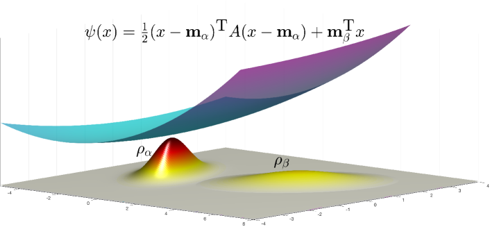
Gelbrich provides a more general result than that provided in Remark 2.31: the Bures metric between Gaussians extends more generally to elliptically contoured distributions (1990). In a nutshell, one can first show that for two measures with given mean and covariance matrices, the distance between the two Gaussians with these respective parameters is a lower bound of the Wasserstein distance between the two measures (Gelbrich, 1990, Theorem 2.1). Additionally, the closed form (2.41) extends to families of elliptically contoured densities: If two densities ραsubscript𝜌𝛼\rho_{\alpha} and ρβsubscript𝜌𝛽\rho_{\beta} belong to such a family, namely when ραsubscript𝜌𝛼\rho_{\alpha} and ρβsubscript𝜌𝛽\rho_{\beta} can be written for any point x𝑥x using a mean and positive definite parameter, ρα(x)=1det(A)h(x𝐦α,A1(x𝐦α))subscript𝜌𝛼𝑥1A𝑥subscript𝐦𝛼superscriptA1𝑥subscript𝐦𝛼\displaystyle\rho_{\alpha}(x)=\frac{1}{\sqrt{\det(\mathrm{\textbf{A}})}}h(\langle x-\mathbf{m}_{\alpha},\,\mathrm{\textbf{A}}^{-1}(x-\mathbf{m}_{\alpha})\rangle) ρβ(x)=1det(B)h(x𝐦β,B1(x𝐦β)),subscript𝜌𝛽𝑥1B𝑥subscript𝐦𝛽superscriptB1𝑥subscript𝐦𝛽\displaystyle\rho_{\beta}(x)=\frac{1}{\sqrt{\det(\mathrm{\textbf{B}})}}h(\langle x-\mathbf{m}_{\beta},\,\mathrm{\textbf{B}}^{-1}(x-\mathbf{m}_{\beta})\rangle), for the same nonnegative valued function hh such that the integral dh(x,x)𝑑x=1,subscriptsuperscript𝑑𝑥𝑥differential-d𝑥1\int_{\mathbb{R}^{d}}h(\langle x,\,x\rangle)dx=1, then their optimal transport map is also the linear map (2.40) and their Wasserstein distance is also given by the expression (2.41)italic-(2.41italic-)\eqref{eq-dist-gauss}, with a slightly different scaling of the Bures metric that depends only the generator function hh. For instance, that scaling is 111 for Gaussians (h(t)=et/2𝑡superscript𝑒𝑡2h(t)=e^{-t/2}) and 1/(d+2)1𝑑21/(d+2) for uniform distributions on ellipsoids (hh the indicator function for [0,1]01[0,1]). This result follows from the fact that the covariance matrix of an elliptic distribution is a constant times its positive definite parameter (Gómez et al., 2003, Theo. 4(ii)) and that the Wasserstein distance between elliptic distributions is a function of the Bures distance between their covariance matrices (Gelbrich, 1990, Cor. 2.5).
Refer to caption
Figure 2.13: Same Gaussians ραsubscript𝜌𝛼\rho_{\alpha} and ρβsubscript𝜌𝛽\rho_{\beta} as defined in Figure 2.12, represented this time as surfaces. The surface above is the Brenier potential ψ𝜓\psi defined up to an additive constant (here +50) such that T=ψ𝑇𝜓T=\nabla\psi. For visual purposes, both Gaussian densities have been multiplied by a factor of 100.
Refer to caption Refer to caption
Figure 2.14: Computation of displacement interpolation between two 1-D Gaussians. Denoting 𝒢m,σ(x)=def.12πse(xm)22s2superscriptdef.subscript𝒢𝑚𝜎𝑥12𝜋𝑠superscript𝑒superscript𝑥𝑚22superscript𝑠2\mathcal{G}_{m,\sigma}(x)\stackrel{{\scriptstyle\mbox{\tiny def.}}}{{=}}\frac{1}{\sqrt{2\pi}s}e^{-\frac{(x-m)^{2}}{2s^{2}}} the Gaussian density, it thus shows the interpolation 𝒢(1t)m0+tm1,(1t)σ0+tσ1subscript𝒢1𝑡subscript𝑚0𝑡subscript𝑚11𝑡subscript𝜎0𝑡subscript𝜎1\mathcal{G}_{(1-t)m_{0}+tm_{1},(1-t)\sigma_{0}+t\sigma_{1}}.

Chapter 3 Algorithmic Foundations

This chapter describes the most common algorithmic tools from combinatorial optimization and linear programming that can be used to solve the discrete formulation of optimal transport, as described in the primal problem (2.11) or alternatively its dual (2.20).

The origins of these algorithms can be traced back to World War II, either right before with Tolstoı’s seminal work (1930) or during the war itself, when Hitchcock (1941) and Kantorovich (1942) formalized the generic problem of dispatching available resources toward consumption sites in an optimal way. Both of these formulations, as well as the later contribution by Koopmans (1949), fell short of providing a provably correct algorithm to solve that problem (the cycle violation method was already proposed as a heuristic by Tolstoı (1939)). One had to wait until the field of linear programming fully blossomed, with the proposal of the simplex method, to be at last able to solve rigorously these problems.

The goal of linear programming is to solve optimization problems whose objective function is linear and whose constraints are linear (in)equalities in the variables of interest. The optimal transport problem fits that description and is therefore a particular case of that wider class of problems. One can argue, however, that optimal transport is truly special among all linear program. First, Dantzig’s early motivation to solve linear programs was greatly related to that of solving transportation problems (Dantzig, 1949, p. 210). Second, despite being only a particular case, the optimal transport problem remained in the spotlight of optimization, because it was understood shortly after that optimal transport problems were related, and in fact equivalent, to an important class of linear programs known as minimum cost network flows (Korte and Vygen, 2012, p. 213, Lem. 9.3) thanks to a result by Ford and Fulkerson (1962). As such, the OT problem has been the subject of particular attention, ever since the birth of mathematical programming (Dantzig, 1951), and is still widely used to introduce optimization to a new audience (Nocedal and Wright, 1999, §1, p. 4).

3.1 The Kantorovich Linear Programs

We have already introduced in Equation (2.11) the primal OT problem:

LC(a,b)=minPU(a,b)in,jmCi,jPi,j.subscriptLCabPUabsubscript𝑖delimited-⟦⟧𝑛𝑗delimited-⟦⟧𝑚subscriptC𝑖𝑗subscriptP𝑖𝑗\mathrm{L}_{\mathrm{\textbf{C}}}(\mathrm{\textbf{a}},\mathrm{\textbf{b}})=\underset{\mathrm{\textbf{P}}\in\mathrm{\textbf{U}}(\mathrm{\textbf{a}},\mathrm{\textbf{b}})}{\min}\;\sum_{i\in\llbracket n\rrbracket,j\in\llbracket m\rrbracket}\mathrm{\textbf{C}}_{i,j}\mathrm{\textbf{P}}_{i,j}. (3.1)

To make the link with the linear programming literature, one can cast the equation above as a linear program in standard form, that is, a linear program with a linear objective; equality constraints defined with a matrix and a constant vector; and nonnegative constraints on variables. Let 𝕀nsubscript𝕀𝑛\mathbb{I}_{n} stand for the identity matrix of size n𝑛n and let tensor-product\otimes be Kronecker’s product. The (n+m)×nm𝑛𝑚𝑛𝑚{(n+m)\times nm} matrix

𝐀=[𝟙nT𝕀m𝕀n𝟙mT](n+m)×nm𝐀matrixtensor-productsuperscriptsubscriptdouble-struck-𝟙𝑛Tsubscript𝕀𝑚tensor-productsubscript𝕀𝑛superscriptsubscriptdouble-struck-𝟙𝑚Tsuperscript𝑛𝑚𝑛𝑚\mathbf{A}=\begin{bmatrix}{\mathbb{1}_{n}}^{\mathrm{T}}\otimes\mathbb{I}_{m}\\ \mathbb{I}_{n}\otimes{\mathbb{1}_{m}}^{\mathrm{T}}\end{bmatrix}\in\mathbb{R}^{(n+m)\times nm}

can be used to encode the row-sum and column-sum constraints that need to be satisfied for any P to be in U(a,b)Uab\mathrm{\textbf{U}}(\mathrm{\textbf{a}},\mathrm{\textbf{b}}). To do so, simply cast a matrix Pn×mPsuperscript𝑛𝑚\mathrm{\textbf{P}}\in\mathbb{R}^{n\times m} as a vector pnmpsuperscript𝑛𝑚\mathrm{\textbf{p}}\in\mathbb{R}^{nm} such that the i+n(j1)𝑖𝑛𝑗1i+n(j-1)’s element of p is equal to PijsubscriptP𝑖𝑗\mathrm{\textbf{P}}_{ij} (P is enumerated columnwise) to obtain the following equivalence:

Pn×mU(a,b)p+nm,𝐀p=[ab].Psuperscript𝑛𝑚Uabformulae-sequencepsubscriptsuperscript𝑛𝑚𝐀pdelimited-[]ab\mathrm{\textbf{P}}\in\mathbb{R}^{n\times m}\in\mathrm{\textbf{U}}(\mathrm{\textbf{a}},\mathrm{\textbf{b}})\Leftrightarrow\mathrm{\textbf{p}}\in\mathbb{R}^{nm}_{+},\mathbf{A}\mathrm{\textbf{p}}=\bigl{[}\begin{smallmatrix}\mathrm{\textbf{a}}\\ \mathrm{\textbf{b}}\end{smallmatrix}\bigr{]}.

Therefore we can write the original optimal transport problem as

LC(a,b)=minp+nm𝐀p=[ab]cTp,subscriptLCabpsubscriptsuperscript𝑛𝑚𝐀pdelimited-[]absuperscriptcTp\mathrm{L}_{\mathrm{\textbf{C}}}(\mathrm{\textbf{a}},\mathrm{\textbf{b}})=\underset{\begin{subarray}{c}\mathrm{\textbf{p}}\in\mathbb{R}^{nm}_{+}\\ \mathbf{A}\mathrm{\textbf{p}}=\bigl{[}\begin{smallmatrix}\mathrm{\textbf{a}}\\ \mathrm{\textbf{b}}\end{smallmatrix}\bigr{]}\end{subarray}}{\min}\;{\mathrm{\textbf{c}}}^{\mathrm{T}}\mathrm{\textbf{p}}, (3.2)

where the nm𝑛𝑚nm-dimensional vector c is equal to the stacked columns contained in the cost matrix C.

Remark 3.1.

Note that one of the n+m𝑛𝑚n+m constraints described above is redundant or that, in other words, the line vectors of matrix A𝐴A are not linearly independent. Indeed, summing all n𝑛n first lines and the subsequent m𝑚m lines results in the same vector (namely A[𝟙n𝟘m]=A[𝟘n𝟙m]=𝟙nmT𝐴delimited-[]subscriptdouble-struck-𝟙𝑛subscriptdouble-struck-𝟘𝑚𝐴delimited-[]subscriptdouble-struck-𝟘𝑛subscriptdouble-struck-𝟙𝑚superscriptsubscriptdouble-struck-𝟙𝑛𝑚TA\bigl{[}\begin{smallmatrix}\mathbb{1}_{n}\\ \mathbb{0}_{m}\end{smallmatrix}\bigr{]}=A\bigl{[}\begin{smallmatrix}\mathbb{0}_{n}\\ \mathbb{1}_{m}\end{smallmatrix}\bigr{]}={\mathbb{1}_{nm}}^{\mathrm{T}}). One can show that removing a line in A𝐴A and the corresponding entry in [ab]delimited-[]ab\bigl{[}\begin{smallmatrix}\mathrm{\textbf{a}}\\ \mathrm{\textbf{b}}\end{smallmatrix}\bigr{]} yields a properly defined linear system. For simplicity, and to avoid treating asymmetrically a and b, we retain in what follows a redundant formulation, keeping in mind that degeneracy will pop up in some of our computations.

The dual problem corresponding to Equation (3.2) is, following duality in linear programming (Bertsimas and Tsitsiklis, 1997, p. 143) defined as

LC(a,b)=maxhn+mAThc[ab]Th.subscriptLCabhsuperscript𝑛𝑚superscript𝐴Thcsuperscriptdelimited-[]abTh\mathrm{L}_{\mathrm{\textbf{C}}}(\mathrm{\textbf{a}},\mathrm{\textbf{b}})=\underset{\begin{subarray}{c}\mathrm{\textbf{h}}\in\mathbb{R}^{n+m}\\ {A}^{\mathrm{T}}\mathrm{\textbf{h}}\leq\mathrm{\textbf{c}}\end{subarray}}{\max}\;{\bigl{[}\begin{smallmatrix}\mathrm{\textbf{a}}\\ \mathrm{\textbf{b}}\end{smallmatrix}\bigr{]}}^{\mathrm{T}}\mathrm{\textbf{h}}. (3.3)

Note that this program is exactly equivalent to that presented in Equation (2.4).

Remark 3.2.

We provide a simple derivation of the duality result above, which can be seen as a direct formulation of the arguments developed in Remark 2.21. Strong duality, namely the fact that the optima of both primal (3.2) and dual (3.3) problems do indeed coincide, requires a longer proof (Bertsimas and Tsitsiklis, 1997, §4.10). To simplify notation, we write q=[ab]qdelimited-[]ab\mathrm{\textbf{q}}=\bigl{[}\begin{smallmatrix}\mathrm{\textbf{a}}\\ \mathrm{\textbf{b}}\end{smallmatrix}\bigr{]}. Consider now a relaxed primal problem of the optimal transport problem, where the constraint 𝐀p=q𝐀pq\mathbf{A}\mathrm{\textbf{p}}=\mathrm{\textbf{q}} is no longer necessarily enforced but bears instead a cost hT(𝐀pq)superscripthT𝐀pq{\mathrm{\textbf{h}}}^{\mathrm{T}}(\mathbf{A}\mathrm{\textbf{p}}-\mathrm{\textbf{q}}) parameterized by an arbitrary vector of costs hn+mhsuperscript𝑛𝑚\mathrm{\textbf{h}}\in\mathbb{R}^{n+m}. This relaxation, whose optimum depends directly on the cost vector h, can be written as

H(h)=def.minp+nmcTphT(𝐀pq).superscriptdef.Hhpsubscriptsuperscript𝑛𝑚superscriptcTpsuperscripthT𝐀pq\mathrm{H}(\mathrm{\textbf{h}})\stackrel{{\scriptstyle\mbox{\tiny def.}}}{{=}}\underset{\mathrm{\textbf{p}}\in\mathbb{R}^{nm}_{+}}{\min}\;{\mathrm{\textbf{c}}}^{\mathrm{T}}\mathrm{\textbf{p}}-{\mathrm{\textbf{h}}}^{\mathrm{T}}(\mathbf{A}\mathrm{\textbf{p}}-\mathrm{\textbf{q}}).

Note first that this relaxed problem has no marginal constraints on p. Because that minimization allows for many more p solutions, we expect H(h)Hh\mathrm{H}(\mathrm{\textbf{h}}) to be smaller than z¯=LC(a,b)¯𝑧subscriptLCab\bar{z}=\mathrm{L}_{\mathrm{\textbf{C}}}(\mathrm{\textbf{a}},\mathrm{\textbf{b}}). Indeed, writing psuperscriptp\mathrm{\textbf{p}}^{\star} for any optimal solution of the primal problem (3.1), we obtain

minp+nmcTphT(𝐀pq)cTphT(𝐀pq)=cTp=z¯.psubscriptsuperscript𝑛𝑚superscriptcTpsuperscripthT𝐀pqsuperscriptcTsuperscriptpsuperscripthT𝐀superscriptpqsuperscriptcTsuperscriptp¯𝑧\underset{\mathrm{\textbf{p}}\in\mathbb{R}^{nm}_{+}}{\min}\;{\mathrm{\textbf{c}}}^{\mathrm{T}}\mathrm{\textbf{p}}-{\mathrm{\textbf{h}}}^{\mathrm{T}}(\mathbf{A}\mathrm{\textbf{p}}-\mathrm{\textbf{q}})\leq{\mathrm{\textbf{c}}}^{\mathrm{T}}\mathrm{\textbf{p}}^{\star}-{\mathrm{\textbf{h}}}^{\mathrm{T}}(\mathbf{A}\mathrm{\textbf{p}}^{\star}-\mathrm{\textbf{q}})={\mathrm{\textbf{c}}}^{\mathrm{T}}\mathrm{\textbf{p}}^{\star}=\bar{z}.

The approach above defines therefore a problem which can be used to compute an optimal upper bound for the original problem (3.1), for any cost vector h; that function is called the Lagrange dual function of LL\mathrm{L}. The goal of duality theory is now to compute the best lower bound z¯¯𝑧\underline{z} by maximizing HH\mathrm{H} over any cost vector h, namely

z¯=maxh(H(h)=maxhhTq+minp+nm(cATh)Tp).¯𝑧hHhhsuperscripthTqpsubscriptsuperscript𝑛𝑚superscriptcsuperscript𝐴ThTp\underline{z}=\underset{\mathrm{\textbf{h}}}{\max}\;\left(\mathrm{H}(\mathrm{\textbf{h}})=\underset{\mathrm{\textbf{h}}}{\max}\;{\mathrm{\textbf{h}}}^{\mathrm{T}}\mathrm{\textbf{q}}+\underset{\mathrm{\textbf{p}}\in\mathbb{R}^{nm}_{+}}{\min}\;{(\mathrm{\textbf{c}}-{A}^{\mathrm{T}}\mathrm{\textbf{h}})}^{\mathrm{T}}\mathrm{\textbf{p}}\right).

The second term involving a minimization on p can be easily shown to be -\infty if any coordinate of cTAThsuperscriptcTsuperscript𝐴Th{\mathrm{\textbf{c}}}^{\mathrm{T}}-{A}^{\mathrm{T}}\mathrm{\textbf{h}} is negative. Indeed, if for instance for a given index in+m𝑖𝑛𝑚i\leq n+m we have ci(ATh)i<0subscriptc𝑖subscriptsuperscript𝐴Th𝑖0\mathrm{\textbf{c}}_{i}-({A}^{\mathrm{T}}\mathrm{\textbf{h}})_{i}<0, then it suffices to take for p the canonical vector eisubscripte𝑖\mathrm{\textbf{e}}_{i} multiplied by any arbitrary large positive value to obtain an unbounded value. When trying to maximize the lower bound H(h)Hh\mathrm{H}(\mathrm{\textbf{h}}) it therefore makes sense to restrict vectors h to be such that AThcsuperscript𝐴Thc{A}^{\mathrm{T}}\mathrm{\textbf{h}}\leq\mathrm{\textbf{c}}, in which case the best possible lower bound becomes

z¯=maxhn+mAThchTq.¯𝑧hsuperscript𝑛𝑚superscript𝐴ThcsuperscripthTq\underline{z}=\underset{\begin{subarray}{c}\mathrm{\textbf{h}}\in\mathbb{R}^{n+m}\\ {A}^{\mathrm{T}}\mathrm{\textbf{h}}\leq\mathrm{\textbf{c}}\end{subarray}}{\max}\;{\mathrm{\textbf{h}}}^{\mathrm{T}}\mathrm{\textbf{q}}.

We have therefore proved a weak duality result, namely that z¯z¯¯𝑧¯𝑧\underline{z}\leq\bar{z}.

3.2 C-Transforms

We present in this section an important property of the dual optimal transport problem (3.3) which takes a more important meaning when used for the semidiscrete optimal transport problem in §5.1. This section builds upon the original formulation (2.20) that splits dual variables according to row and column sum constraints:

LC(a,b)=max(f,g)R(C)f,a+g,b.subscriptLCabfgRCfagb\mathrm{L}_{\mathrm{\textbf{C}}}(\mathrm{\textbf{a}},\mathrm{\textbf{b}})=\underset{(\mathrm{\textbf{f}},\mathrm{\textbf{g}})\in\mathrm{\textbf{R}}(\mathrm{\textbf{C}})}{\max}\;\langle\mathrm{\textbf{f}},\,\mathrm{\textbf{a}}\rangle+\langle\mathrm{\textbf{g}},\,\mathrm{\textbf{b}}\rangle. (3.4)

Consider any dual feasible pair (f,g)fg(\mathrm{\textbf{f}},\mathrm{\textbf{g}}). If we “freeze” the value of f, we can notice that there is no better vector solution for g than the C-transform vector of f, denoted fCmsuperscriptfCsuperscript𝑚\mathrm{\textbf{f}}^{\,\mathrm{\textbf{C}}}\in\mathbb{R}^{m} and defined as

(fC)j=mininCijfi,subscriptsuperscriptfC𝑗subscript𝑖delimited-⟦⟧𝑛subscriptC𝑖𝑗subscriptf𝑖(\mathrm{\textbf{f}}^{\,\mathrm{\textbf{C}}})_{j}=\min_{i\in\llbracket n\rrbracket}\mathrm{\textbf{C}}_{ij}-\mathrm{\textbf{f}}_{i},

since it is indeed easy to prove that (f,fC)R(C)fsuperscriptfCRC(\mathrm{\textbf{f}},\mathrm{\textbf{f}}^{\,\mathrm{\textbf{C}}})\in\mathrm{\textbf{R}}(\mathrm{\textbf{C}}) and that fCsuperscriptfC\mathrm{\textbf{f}}^{\,\mathrm{\textbf{C}}} is the largest possible vector such that this constraint is satisfied. We therefore have that

f,a+g,bf,a+fC,b.fagbfasuperscriptfCb\langle\mathrm{\textbf{f}},\,\mathrm{\textbf{a}}\rangle+\langle\mathrm{\textbf{g}},\,\mathrm{\textbf{b}}\rangle\leq\langle\mathrm{\textbf{f}},\,\mathrm{\textbf{a}}\rangle+\langle\mathrm{\textbf{f}}^{\,\mathrm{\textbf{C}}},\,\mathrm{\textbf{b}}\rangle.

This result allows us first to reformulate the dual problem as a piecewise affine concave maximization problem expressed in a single variable f as

LC(a,b)=maxfnf,a+fC,b.subscriptLCabfsuperscript𝑛fasuperscriptfCb\mathrm{L}_{\mathrm{\textbf{C}}}(\mathrm{\textbf{a}},\mathrm{\textbf{b}})=\underset{\mathrm{\textbf{f}}\in\mathbb{R}^{n}}{\max}\;\langle\mathrm{\textbf{f}},\,\mathrm{\textbf{a}}\rangle+\langle\mathrm{\textbf{f}}^{\,\mathrm{\textbf{C}}},\,\mathrm{\textbf{b}}\rangle. (3.5)

Putting that result aside, the same reasoning applies of course if we now “freeze” the values of g and consider instead the C¯¯C\bar{\mathrm{\textbf{C}}}-transform of g, namely vector gC¯nsuperscriptg¯Csuperscript𝑛\mathrm{\textbf{g}}^{\bar{\mathrm{\textbf{C}}}}\in\mathbb{R}^{n} defined as

(gC¯)i=minjmCijgj,subscriptsuperscriptg¯C𝑖subscript𝑗delimited-⟦⟧𝑚subscriptC𝑖𝑗subscriptg𝑗(\mathrm{\textbf{g}}^{\bar{\mathrm{\textbf{C}}}})_{i}=\min_{j\in\llbracket m\rrbracket}\mathrm{\textbf{C}}_{ij}-\mathrm{\textbf{g}}_{j},

with a different increase in objective

f,a+g,bgC¯,a+g,b.fagbsuperscriptg¯Cagb\langle\mathrm{\textbf{f}},\,\mathrm{\textbf{a}}\rangle+\langle\mathrm{\textbf{g}},\,\mathrm{\textbf{b}}\rangle\leq\langle\mathrm{\textbf{g}}^{\bar{\mathrm{\textbf{C}}}},\,\mathrm{\textbf{a}}\rangle+\langle\mathrm{\textbf{g}},\,\mathrm{\textbf{b}}\rangle.

Starting from a given f, it is therefore tempting to alternate C and C¯¯C\bar{\mathrm{\textbf{C}}} transforms several times to improve f. Indeed, we have the sequence of inequalities

f,a+fC,bfCC¯,a+fC,bfCC¯,a+fCC¯C,bfasuperscriptfCbsuperscriptfC¯CasuperscriptfCbsuperscriptfC¯CasuperscriptfC¯CCb\langle\mathrm{\textbf{f}},\,\mathrm{\textbf{a}}\rangle+\langle\mathrm{\textbf{f}}^{\,\mathrm{\textbf{C}}},\,\mathrm{\textbf{b}}\rangle\leq\langle\mathrm{\textbf{f}}^{\,\mathrm{\textbf{C}}\bar{\mathrm{\textbf{C}}}},\,\mathrm{\textbf{a}}\rangle+\langle\mathrm{\textbf{f}}^{\,\mathrm{\textbf{C}}},\,\mathrm{\textbf{b}}\rangle\leq\langle\mathrm{\textbf{f}}^{\,\mathrm{\textbf{C}}\bar{\mathrm{\textbf{C}}}},\,\mathrm{\textbf{a}}\rangle+\langle\mathrm{\textbf{f}}^{\,\mathrm{\textbf{C}}\bar{\mathrm{\textbf{C}}}\mathrm{\textbf{C}}},\,\mathrm{\textbf{b}}\rangle\leq\dots

One may hope for a strict increase in the objective at each of these iterations. However, this does not work because alternating C and C¯¯C\bar{\mathrm{\textbf{C}}} transforms quickly hits a plateau.

Proposition 3.1.

The following identities, in which the inequality sign between vectors should be understood elementwise, hold:

  1. (i)

    fffCfCfsuperscriptfsuperscriptfCsuperscriptfC\mathrm{\textbf{f}}\leq\mathrm{\textbf{f}}\,^{\prime}\Rightarrow\mathrm{\textbf{f}}^{\,\mathrm{\textbf{C}}}\geq\mathrm{\textbf{f}}\,^{\prime\,\mathrm{\textbf{C}}},

  2. (ii)

    fCC¯fsuperscriptfC¯Cf\mathrm{\textbf{f}}^{\,\mathrm{\textbf{C}}\bar{\mathrm{\textbf{C}}}}\geq\mathrm{\textbf{f}}, gC¯Cgsuperscriptg¯CCg\mathrm{\textbf{g}}^{\bar{\mathrm{\textbf{C}}}\mathrm{\textbf{C}}}\geq\mathrm{\textbf{g}},

  3. (iii)

    fCC¯C=fC.superscriptfC¯CCsuperscriptfC\mathrm{\textbf{f}}^{\,\mathrm{\textbf{C}}\bar{\mathrm{\textbf{C}}}\mathrm{\textbf{C}}}=\mathrm{\textbf{f}}^{\,\mathrm{\textbf{C}}}.

Proof.

The first inequality follows from the definition of C-transforms. Expanding the definition of fCC¯superscriptfC¯C\mathrm{\textbf{f}}^{\,\mathrm{\textbf{C}}\bar{\mathrm{\textbf{C}}}} we have

(fCC¯)i=minjmCijfjC=minjmCijmininCijfi.subscriptsuperscriptfC¯C𝑖subscript𝑗delimited-⟦⟧𝑚subscriptC𝑖𝑗subscriptsuperscriptfC𝑗subscript𝑗delimited-⟦⟧𝑚subscriptC𝑖𝑗subscriptsuperscript𝑖delimited-⟦⟧𝑛subscriptCsuperscript𝑖𝑗subscriptfsuperscript𝑖\left(\mathrm{\textbf{f}}^{\,\mathrm{\textbf{C}}\bar{\mathrm{\textbf{C}}}}\right)_{i}=\min_{j\in\llbracket m\rrbracket}\mathrm{\textbf{C}}_{ij}-\mathrm{\textbf{f}}^{\,\mathrm{\textbf{C}}}_{j}=\min_{j\in\llbracket m\rrbracket}\mathrm{\textbf{C}}_{ij}-\min_{i^{\prime}\in\llbracket n\rrbracket}\mathrm{\textbf{C}}_{i^{\prime}j}-\mathrm{\textbf{f}}_{i^{\prime}}.

Now, since mininCijfi(Cijfi)subscriptsuperscript𝑖delimited-⟦⟧𝑛subscriptCsuperscript𝑖𝑗subscriptfsuperscript𝑖subscriptC𝑖𝑗subscriptf𝑖-\min_{i^{\prime}\in\llbracket n\rrbracket}\mathrm{\textbf{C}}_{i^{\prime}j}-\mathrm{\textbf{f}}_{i^{\prime}}\geq-(\mathrm{\textbf{C}}_{ij}-\mathrm{\textbf{f}}_{i}), we recover

(fCC¯)iminjmCijCij+fi=fi.subscriptsuperscriptfC¯C𝑖subscript𝑗delimited-⟦⟧𝑚subscriptC𝑖𝑗subscriptC𝑖𝑗subscriptf𝑖subscriptf𝑖\left(\mathrm{\textbf{f}}^{\,\mathrm{\textbf{C}}\bar{\mathrm{\textbf{C}}}}\right)_{i}\geq\min_{j\in\llbracket m\rrbracket}\mathrm{\textbf{C}}_{ij}-\mathrm{\textbf{C}}_{ij}+\mathrm{\textbf{f}}_{i}=\mathrm{\textbf{f}}_{i}.

The relation gC¯Cgsuperscriptg¯CCg\mathrm{\textbf{g}}^{\bar{\mathrm{\textbf{C}}}\mathrm{\textbf{C}}}\geq\mathrm{\textbf{g}} is obtained in the same way. Now, set g=fCgsuperscriptfC\mathrm{\textbf{g}}=\mathrm{\textbf{f}}^{\,\mathrm{\textbf{C}}}. Then, gC¯=fCC¯fsuperscriptg¯CsuperscriptfC¯Cf\mathrm{\textbf{g}}^{\bar{\mathrm{\textbf{C}}}}=\mathrm{\textbf{f}}^{\,\mathrm{\textbf{C}}\bar{\mathrm{\textbf{C}}}}\geq\mathrm{\textbf{f}}. Therefore, using result (i) we have fCC¯CfCsuperscriptfC¯CCsuperscriptfC\mathrm{\textbf{f}}^{\,\mathrm{\textbf{C}}\bar{\mathrm{\textbf{C}}}\mathrm{\textbf{C}}}\leq\mathrm{\textbf{f}}^{\,\mathrm{\textbf{C}}}. Result (ii) yields fCC¯CfCsuperscriptfC¯CCsuperscriptfC\mathrm{\textbf{f}}^{\,\mathrm{\textbf{C}}\bar{\mathrm{\textbf{C}}}\mathrm{\textbf{C}}}\geq\mathrm{\textbf{f}}^{\,\mathrm{\textbf{C}}}, proving the equality. ∎

3.3 Complementary Slackness

Primal (3.2) and dual (3.3), (2.20) problems can be solved independently to obtain optimal primal PsuperscriptP\mathrm{\textbf{P}}^{\star} and dual (f,g)superscriptfsuperscriptg(\mathrm{\textbf{f}}^{\star},\mathrm{\textbf{g}}^{\star}) solutions. The following proposition characterizes their relationship.

Proposition 3.2.

Let PsuperscriptP\mathrm{\textbf{P}}^{\star} and f,gsuperscriptfsuperscriptg\mathrm{\textbf{f}}^{\star},\mathrm{\textbf{g}}^{\star} be optimal solutions for the primal (2.24) and dual (2.11) problems, respectively. Then, for any pair (i,j)n×m(i,j)\in\llbracket n\rrbracket\times\llbracket m\rrbracket, Pi,j(Ci,jfi+gj)=0subscriptsuperscriptP𝑖𝑗subscriptC𝑖𝑗subscriptsuperscriptf𝑖subscriptsuperscriptg𝑗0\mathrm{\textbf{P}}^{\star}_{i,j}(\mathrm{\textbf{C}}_{i,j}-\mathrm{\textbf{f}}^{\star}_{i}+\mathrm{\textbf{g}}^{\star}_{j})=0 holds. In other words, if Pi,j>0subscriptsuperscriptP𝑖𝑗0\mathrm{\textbf{P}}^{\star}_{i,j}>0, then necessarily fi+gj=Ci,jsubscriptsuperscriptf𝑖subscriptsuperscriptg𝑗subscriptC𝑖𝑗\mathrm{\textbf{f}}^{\star}_{i}+\mathrm{\textbf{g}}^{\star}_{j}=\mathrm{\textbf{C}}_{i,j}; if fi+gj<Ci,jsubscriptsuperscriptf𝑖subscriptsuperscriptg𝑗subscriptC𝑖𝑗\mathrm{\textbf{f}}^{\star}_{i}+\mathrm{\textbf{g}}^{\star}_{j}<\mathrm{\textbf{C}}_{i,j} then necessarily Pi,j=0subscriptsuperscriptP𝑖𝑗0\mathrm{\textbf{P}}^{\star}_{i,j}=0.

Proof.

We have by strong duality that P,C=f,a+g,bsuperscriptPCsuperscriptfasuperscriptgb\langle\mathrm{\textbf{P}}^{\star},\,\mathrm{\textbf{C}}\rangle=\langle\mathrm{\textbf{f}}^{\star},\,\mathrm{\textbf{a}}\rangle+\langle\mathrm{\textbf{g}}^{\star},\,\mathrm{\textbf{b}}\rangle. Recall that P𝟙m=asuperscriptPsubscriptdouble-struck-𝟙𝑚a\mathrm{\textbf{P}}^{\star}\mathbb{1}_{m}=\mathrm{\textbf{a}} and PT𝟙n=bsuperscriptsuperscriptPTsubscriptdouble-struck-𝟙𝑛b{\mathrm{\textbf{P}}^{\star}}^{\mathrm{T}}\mathbb{1}_{n}=\mathrm{\textbf{b}}; therefore

f,a+g,bsuperscriptfasuperscriptgb\displaystyle\langle\mathrm{\textbf{f}}^{\star},\,\mathrm{\textbf{a}}\rangle+\langle\mathrm{\textbf{g}}^{\star},\,\mathrm{\textbf{b}}\rangle =f,P𝟙m+g,PT𝟙nabsentsuperscriptfsuperscriptPsubscriptdouble-struck-𝟙𝑚superscriptgsuperscriptsuperscriptPTsubscriptdouble-struck-𝟙𝑛\displaystyle=\langle\mathrm{\textbf{f}}^{\star},\,\mathrm{\textbf{P}}^{\star}\mathbb{1}_{m}\rangle+\langle\mathrm{\textbf{g}}^{\star},\,{\mathrm{\textbf{P}}^{\star}}^{\mathrm{T}}\mathbb{1}_{n}\rangle
=f𝟙mT,P+𝟙ngT,P,absentsuperscriptfsuperscriptsubscriptdouble-struck-𝟙𝑚TsuperscriptPsubscriptdouble-struck-𝟙𝑛superscriptsuperscriptgTsuperscriptP\displaystyle=\langle\mathrm{\textbf{f}}^{\star}{\mathbb{1}_{m}}^{\mathrm{T}},\,\mathrm{\textbf{P}}^{\star}\rangle+\langle\mathbb{1}_{n}{\mathrm{\textbf{g}}^{\star}}^{\mathrm{T}},\,\mathrm{\textbf{P}}^{\star}\rangle,

which results in

P,Cfg=0.superscriptPdirect-sumCsuperscriptfsuperscriptg0\langle\mathrm{\textbf{P}}^{\star},\,\mathrm{\textbf{C}}-\mathrm{\textbf{f}}^{\star}\oplus\mathrm{\textbf{g}}^{\star}\rangle=0.

Because (f,g)superscriptfsuperscriptg(\mathrm{\textbf{f}}^{\star},\mathrm{\textbf{g}}^{\star}) belongs to the polyhedron of dual constraints (2.21), each entry of the matrix Cfgdirect-sumCsuperscriptfsuperscriptg\mathrm{\textbf{C}}-\mathrm{\textbf{f}}^{\star}\oplus\mathrm{\textbf{g}}^{\star} is necessarily nonnegative. Therefore, since all the entries of P are nonnegative, the constraint that the dot-product above is equal to 00 enforces that, for any pair of indices (i,j)𝑖𝑗(i,j) such that Pi,j>0subscriptP𝑖𝑗0\mathrm{\textbf{P}}_{i,j}>0, Ci,j(fi+gj)subscriptC𝑖𝑗subscriptf𝑖subscriptg𝑗\mathrm{\textbf{C}}_{i,j}-(\mathrm{\textbf{f}}_{i}+\mathrm{\textbf{g}}_{j}) must be zero, and for any pair of indices (i,j)𝑖𝑗(i,j) such that Ci,j>fi+gjsubscriptC𝑖𝑗subscriptf𝑖subscriptg𝑗\mathrm{\textbf{C}}_{i,j}>\mathrm{\textbf{f}}_{i}+\mathrm{\textbf{g}}_{j} that Pi,j=0subscriptP𝑖𝑗0\mathrm{\textbf{P}}_{i,j}=0. ∎

The converse result is also true. We define first the idea that two variables for the primal and dual problems are complementary.

Definition 3.1.

A matrix Pn×mPsuperscript𝑛𝑚\mathrm{\textbf{P}}\in\mathbb{R}^{n\times m} and a pair of vectors (f,g)fg(\mathrm{\textbf{f}},\mathrm{\textbf{g}}) are complementary w.r.t. C if for all pairs of indices (i,j)𝑖𝑗(i,j) such that Pi,j>0subscriptP𝑖𝑗0\mathrm{\textbf{P}}_{i,j}>0 one also has Ci,j=fi+gjsubscriptC𝑖𝑗subscriptf𝑖subscriptg𝑗\mathrm{\textbf{C}}_{i,j}=\mathrm{\textbf{f}}_{i}+\mathrm{\textbf{g}}_{j}.

If a pair of feasible primal and dual variables is complementary, then we can conclude they are optimal.

Proposition 3.3.

If P and (f,g)fg(\mathrm{\textbf{f}},\mathrm{\textbf{g}}) are complementary and feasible solutions for the primal (2.24) and dual (2.11) problems, respectively, then P and (f,g)fg(\mathrm{\textbf{f}},\mathrm{\textbf{g}}) are both primal and dual optimal.

Proof.

By weak duality, we have that

LC(a,b)P,C=P,fg=a,f+b,gLC(a,b)subscriptLCabPCPdirect-sumfgafbgsubscriptLCab\mathrm{L}_{\mathrm{\textbf{C}}}(\mathrm{\textbf{a}},\mathrm{\textbf{b}})\leq\langle\mathrm{\textbf{P}},\,\mathrm{\textbf{C}}\rangle=\langle\mathrm{\textbf{P}},\,\mathrm{\textbf{f}}\oplus\mathrm{\textbf{g}}\rangle=\langle\mathrm{\textbf{a}},\,\mathrm{\textbf{f}}\rangle+\langle\mathrm{\textbf{b}},\,\mathrm{\textbf{g}}\rangle\leq\mathrm{L}_{\mathrm{\textbf{C}}}(\mathrm{\textbf{a}},\mathrm{\textbf{b}})

and therefore P and (f,g)fg(\mathrm{\textbf{f}},\mathrm{\textbf{g}}) are respectively primal and dual optimal. ∎

3.4 Vertices of the Transportation Polytope

Recall that a vertex or an extremal point of a convex set is formally a point 𝐱𝐱\mathbf{x} in that set such that, if there exiss 𝐲𝐲\mathbf{y} and 𝐳𝐳\mathbf{z} in that set with 𝐱=(𝐲+𝐳)/2𝐱𝐲𝐳2\mathbf{x}=(\mathbf{y}+\mathbf{z})/2, then necessarily 𝐱=𝐲=𝐳𝐱𝐲𝐳\mathbf{x}=\mathbf{y}=\mathbf{z}. A linear program with a nonempty and bounded feasible set attains its minimum at a vertex (or extremal point) of the feasible set (Bertsimas and Tsitsiklis, 1997, p. 65, Theo. 2.7). Since the feasible set U(a,b)Uab\mathrm{\textbf{U}}(\mathrm{\textbf{a}},\mathrm{\textbf{b}}) of the primal optimal transport problem (3.2) is bounded, one can restrict the search for an optimal P to the set of extreme points of the polytope U(a,b)Uab\mathrm{\textbf{U}}(\mathrm{\textbf{a}},\mathrm{\textbf{b}}). Matrices P that are extremal in U(a,b)Uab\mathrm{\textbf{U}}(\mathrm{\textbf{a}},\mathrm{\textbf{b}}) have an interesting structure that has been the subject of extensive research (Brualdi, 2006, §8). That structure requires describing the transport problem using the formalism of bipartite graphs.

3.4.1 Tree Structure of the Support of All Vertices of U(a,b)Uab\mathrm{\textbf{U}}(\mathrm{\textbf{a}},\mathrm{\textbf{b}})

Let V=(1,2,,n)𝑉12𝑛V=(1,2,\dots,n) and V=(1,2,,m)superscript𝑉superscript1superscript2superscript𝑚V^{\prime}=(1^{\prime},2^{\prime},\dots,m^{\prime}) be two sets of nodes. Note that we add a prime to the labels of set Vsuperscript𝑉V^{\prime} to disambiguate them from those of V𝑉V. Consider their union VV𝑉superscript𝑉V\cup V^{\prime}, with n+m𝑛𝑚n+m nodes, and the set \mathcal{E} of all nm𝑛𝑚nm directed edges {(i,j),in,jm}\{(i,j^{\prime}),i\in\llbracket n\rrbracket,j\in\llbracket m\rrbracket\} between them (here we just add a prime to an integer jm𝑗𝑚j\leq m to form jsuperscript𝑗j^{\prime} in Vsuperscript𝑉V^{\prime}). To each edge (i,j)𝑖superscript𝑗(i,j^{\prime}) we associate the corresponding cost value CijsubscriptC𝑖𝑗\mathrm{\textbf{C}}_{ij}. The complete bipartite graph 𝒢𝒢\mathcal{G} between V𝑉V and Vsuperscript𝑉V^{\prime} is (VV,E)𝑉superscript𝑉𝐸(V\cup V^{\prime},E). A transport plan is a flow on that graph satisfying source (aisubscripta𝑖\mathrm{\textbf{a}}_{i} flowing out of each node i𝑖i) and sink (bjsubscriptb𝑗\mathrm{\textbf{b}}_{j} flowing into each node jsuperscript𝑗j^{\prime}) constraints, as described informally in Figure 3.1. An extremal point in U(a,b)Uab\mathrm{\textbf{U}}(\mathrm{\textbf{a}},\mathrm{\textbf{b}}) has the following property (Brualdi, 2006, p. 338, Theo. 8.1.2).

Refer to caption
Figure 3.1: The optimal transport problem as a bipartite network flow problem. Here n=3,m=4formulae-sequence𝑛3𝑚4n=3,m=4. All coordinates of the source histogram, a, are depicted as source nodes on the left labeled 1,2,31231,2,3, whereas all coordinates of the target histogram b are labeled as nodes 1,2,3,4superscript1superscript2superscript3superscript41^{\prime},2^{\prime},3^{\prime},4^{\prime}. The graph is bipartite in the sense that all source nodes are connected to all target nodes, with no additional edges. To each edge (i,j)𝑖superscript𝑗(i,j^{\prime}) is associated a cost CijsubscriptC𝑖𝑗\mathrm{\textbf{C}}_{ij}. A feasible flow is represented on the right. Proposition 3.4 shows that this flow is not extremal since it has at least one cycle given by ((1,1),(2,1),(2,4),(1,4))1superscript12superscript12superscript41superscript4((1,1^{\prime}),(2,1^{\prime}),(2,4^{\prime}),(1,4^{\prime})).
Refer to caption
Figure 3.2: A solution P with a cycle in the graph of its support can be perturbed to obtain two feasible solutions Q and R such that P is their average, therefore disproving that P is extremal.
Proposition 3.4 (Extremal solutions).

Let P be an extremal point of the polytope U(a,b)Uab\mathrm{\textbf{U}}(\mathrm{\textbf{a}},\mathrm{\textbf{b}}). Let S(P)𝑆PS(\mathrm{\textbf{P}})\subset\mathcal{E} be the subset of edges {(i,j),in,jm such that Pij>0}\{(i,j^{\prime}),i\in\llbracket n\rrbracket,j\in\llbracket m\rrbracket\text{ such that }\mathrm{\textbf{P}}_{ij}>0\}. Then the graph G(P)=def.(VV,S(P))superscriptdef.𝐺P𝑉superscript𝑉𝑆PG(\mathrm{\textbf{P}})\stackrel{{\scriptstyle\mbox{\tiny def.}}}{{=}}(V\cup V^{\prime},S(\mathrm{\textbf{P}})) has no cycles. In particular, P cannot have more than n+m1𝑛𝑚1n+m-1 nonzero entries.

Proof.

We proceed by contradiction. Suppose that P is an extremal point of the polytope U(a,b)Uab\mathrm{\textbf{U}}(\mathrm{\textbf{a}},\mathrm{\textbf{b}}) and that its corresponding set S(P)𝑆PS(\mathrm{\textbf{P}}) of edges, denoted F𝐹F for short, is such that the graph G=(VV,F)𝐺𝑉superscript𝑉𝐹G=(V\cup V^{\prime},F) contains a cycle, namely there exists k>1𝑘1k>1 and a sequence of distinct indices i1,,ik1ni_{1},\dots,i_{k-1}\in\llbracket n\rrbracket and j1,,jk1mj_{1},\dots,j_{k-1}\in\llbracket m\rrbracket such that the set of edges H𝐻H given below forms a subset of F𝐹F.

H={(i1,j1),(i2,j1),(i2,j2),,(ik,jk),(i1,jk)}.𝐻subscript𝑖1superscriptsubscript𝑗1subscript𝑖2superscriptsubscript𝑗1subscript𝑖2superscriptsubscript𝑗2subscript𝑖𝑘superscriptsubscript𝑗𝑘subscript𝑖1superscriptsubscript𝑗𝑘H=\left\{(i_{1},j_{1}^{\prime}),(i_{2},j_{1}^{\prime}),(i_{2},j_{2}^{\prime}),\dots,(i_{k},j_{k}^{\prime}),(i_{1},j_{k}^{\prime})\right\}.

We now construct two feasible matrices Q and R such that P=(Q+R)/2PQR2\mathrm{\textbf{P}}=(\mathrm{\textbf{Q}}+\mathrm{\textbf{R}})/2. To do so, consider a directed cycle H¯¯𝐻\bar{H} corresponding to H𝐻H, namely the sequence of pairs i1j1,j1i2,i2j2,,ikjk,jki1formulae-sequencesubscript𝑖1superscriptsubscript𝑗1formulae-sequencesuperscriptsubscript𝑗1subscript𝑖2formulae-sequencesubscript𝑖2superscriptsubscript𝑗2formulae-sequencesubscript𝑖𝑘superscriptsubscript𝑗𝑘superscriptsubscript𝑗𝑘subscript𝑖1i_{1}\rightarrow j_{1}^{\prime},j_{1}^{\prime}\rightarrow i_{2},i_{2}\rightarrow j_{2}^{\prime},\dots,i_{k}\rightarrow j_{k}^{\prime},j_{k}^{\prime}\rightarrow i_{1}, as well as the elementary amount of flow ε<min(i,j)FPij𝜀subscript𝑖superscript𝑗𝐹subscriptP𝑖𝑗\varepsilon<\min_{(i,j^{\prime})\in F}\mathrm{\textbf{P}}_{ij}. Consider a perturbation matrix 𝐄𝐄\mathbf{E} whose (i,j)𝑖𝑗(i,j) entry is equal to ε𝜀\varepsilon if ijH¯𝑖superscript𝑗¯𝐻i\rightarrow j^{\prime}\in\bar{H}, ε𝜀-\varepsilon if jiH¯𝑗superscript𝑖¯𝐻j\rightarrow i^{\prime}\in\bar{H}, and zero otherwise. Define matrices Q=P+𝐄QP𝐄\mathrm{\textbf{Q}}=\mathrm{\textbf{P}}+\mathbf{E} and R=P𝐄RP𝐄\mathrm{\textbf{R}}=\mathrm{\textbf{P}}-\mathbf{E} as illustrated in Figure 3.2. Because ε𝜀\varepsilon is small enough, all elements in Q and R are nonnegative. By construction, 𝐄𝐄\mathbf{E} has either lines (resp., columns) with all entries equal to 00 or exactly one entry equal to ε𝜀\varepsilon and another equal to ε𝜀-\varepsilon for those indexed by i1,,iksubscript𝑖1subscript𝑖𝑘i_{1},\dots,i_{k} (resp., j1,,jksubscript𝑗1subscript𝑗𝑘j_{1},\dots,j_{k}). Therefore, 𝐄𝐄\mathbf{E} is such that 𝐄𝟙m=𝟘n𝐄subscriptdouble-struck-𝟙𝑚subscriptdouble-struck-𝟘𝑛\mathbf{E}\mathbb{1}_{m}=\mathbb{0}_{n} and 𝐄T𝟙n=𝟘msuperscript𝐄Tsubscriptdouble-struck-𝟙𝑛subscriptdouble-struck-𝟘𝑚{\mathbf{E}}^{\mathrm{T}}\mathbb{1}_{n}=\mathbb{0}_{m}, and we have that Q and R have the same marginals as P, and are therefore feasible. Finally P=(Q+R)/2PQR2\mathrm{\textbf{P}}=(\mathrm{\textbf{Q}}+\mathrm{\textbf{R}})/2 which, since Q,RPQRP\mathrm{\textbf{Q}},\mathrm{\textbf{R}}\neq\mathrm{\textbf{P}}, contradicts the fact that P is an extremal point. Since a graph with k𝑘k nodes and no cycles cannot have more than k1𝑘1k-1 edges, we conclude that S(P)𝑆PS(\mathrm{\textbf{P}}) cannot have more than n+m1𝑛𝑚1n+m-1 edges, and therefore P cannot have more than n+m1𝑛𝑚1n+m-1 nonzero entries. ∎

3.4.2 The North-West Corner Rule

The north-west (NW) corner rule is a heuristic that produces a vertex of the polytope U(a,b)Uab\mathrm{\textbf{U}}(\mathrm{\textbf{a}},\mathrm{\textbf{b}}) in up to n+m𝑛𝑚n+m operations. This heuristic can play a role in initializing any algorithm working on the primal, such as the network simplex outlined in the next section.

The rule starts by giving the highest possible value to P1,1subscriptP11\mathrm{\textbf{P}}_{1,1} by setting it to min(a1,b1)subscripta1subscriptb1\min(\mathrm{\textbf{a}}_{1},\mathrm{\textbf{b}}_{1}). At each step, the entry Pi,jsubscriptP𝑖𝑗\mathrm{\textbf{P}}_{i,j} is chosen to saturate either the row constraint at i𝑖i, the column constraint at j𝑗j, or both if possible. The indices i,j𝑖𝑗i,j are then updated as follows: i𝑖i is incremented in the first case, j𝑗j is in the second, and both i𝑖i and j𝑗j are in the third case. The rule proceeds until Pn,msubscriptP𝑛𝑚\mathrm{\textbf{P}}_{n,m} has received a value.

Formally, the algorithm works as follows: i𝑖i and j𝑗j are initialized to 111, ra1,cb1formulae-sequence𝑟subscripta1𝑐subscriptb1r\leftarrow\mathrm{\textbf{a}}_{1},c\leftarrow\mathrm{\textbf{b}}_{1}. While in𝑖𝑛i\leq n and jm𝑗𝑚j\leq m, set tmin(r,c)𝑡𝑟𝑐t\leftarrow\min(r,c), Pi,jtsubscriptP𝑖𝑗𝑡\mathrm{\textbf{P}}_{i,j}\leftarrow t, rrt𝑟𝑟𝑡r\leftarrow r-t, cst𝑐𝑠𝑡c\leftarrow s-t; if r=0𝑟0r=0 then increment i𝑖i, and update rai𝑟subscripta𝑖r\leftarrow\mathrm{\textbf{a}}_{i} if in𝑖𝑛i\leq n; if c=0𝑐0c=0 then increment j𝑗j, and update cbj𝑐subscriptb𝑗c\leftarrow\mathrm{\textbf{b}}_{j} if jn𝑗𝑛j\leq n; repeat. Here is an example of this sequence assuming a=[0.2,0.5,0.3]a0.20.50.3\mathrm{\textbf{a}}=[0.2,0.5,0.3] and b=[0.5,0.1,0.4]b0.50.10.4\mathrm{\textbf{b}}=[0.5,0.1,0.4]:

[00000000]matrix00000000\displaystyle\begin{bmatrix}\bullet&0&0\\ 0&0&0\\ 0&0&0\end{bmatrix} [0.20000000]absentmatrix0.20000000\displaystyle\rightarrow\begin{bmatrix}0.2&0&0\\ \bullet&0&0\\ 0&0&0\end{bmatrix} [0.2000.30000]absentmatrix0.2000.30000\displaystyle\rightarrow\begin{bmatrix}0.2&0&0\\ 0.3&\bullet&0\\ 0&0&0\end{bmatrix}
[0.2000.30.1000]absentmatrix0.2000.30.1000\displaystyle\rightarrow\begin{bmatrix}0.2&0&0\\ 0.3&0.1&\bullet\\ 0&0&0\end{bmatrix} [0.2000.30.10.100]absentmatrix0.2000.30.10.100\displaystyle\rightarrow\begin{bmatrix}0.2&0&0\\ 0.3&0.1&0.1\\ 0&0&\bullet\end{bmatrix} [0.2000.30.10.1000.3]absentmatrix0.2000.30.10.1000.3\displaystyle\rightarrow\begin{bmatrix}0.2&0&0\\ 0.3&0.1&0.1\\ 0&0&0.3\end{bmatrix}

We write 𝐍𝐖(a,b)𝐍𝐖ab\mathbf{NW}(\mathrm{\textbf{a}},\mathrm{\textbf{b}}) for the unique plan that can be obtained through this heuristic.

Note that there is, however, a much larger number of NW corner solutions that can be obtained by permuting arbitrarily the order of a and b first, computing the corresponding NW corner table, and recovering a table of U(a,b)Uab\mathrm{\textbf{U}}(\mathrm{\textbf{a}},\mathrm{\textbf{b}}) by inverting again the order of columns and rows: setting σ=(3,1,2),σ=(3,2,1)formulae-sequence𝜎312superscript𝜎321\sigma=(3,1,2),\sigma^{\prime}=(3,2,1) gives aσ=[0.3,0.2,0.5],bσ=[0.4,0.1,0.5]formulae-sequencesubscripta𝜎0.30.20.5subscriptbsuperscript𝜎0.40.10.5\mathrm{\textbf{a}}_{\sigma}=[0.3,0.2,0.5],\mathrm{\textbf{b}}_{\sigma^{\prime}}=[0.4,0.1,0.5], and σ1=(2,3,1),σ=(3,2,1)formulae-sequencesuperscript𝜎1231superscript𝜎321\sigma^{-1}=(2,3,1),\sigma^{\prime}=(3,2,1). Observe that

𝐍𝐖(aσ,bσ)=[0.3000.10.10000.5]U(aσ,bσ),𝐍𝐖subscripta𝜎subscriptbsuperscript𝜎matrix0.3000.10.10000.5Usubscripta𝜎subscriptbsuperscript𝜎\displaystyle\mathbf{NW}(\mathrm{\textbf{a}}_{\sigma},\mathrm{\textbf{b}}_{\sigma^{\prime}})=\begin{bmatrix}0.3&0&0\\ 0.1&0.1&0\\ 0&0&0.5\end{bmatrix}\in\mathrm{\textbf{U}}(\mathrm{\textbf{a}}_{\sigma},\mathrm{\textbf{b}}_{\sigma^{\prime}}),
𝐍𝐖σ1σ1(aσ,bσ)=[00.10.10.500000.3]U(a,b).subscript𝐍𝐖superscript𝜎1superscript𝜎1subscripta𝜎subscriptbsuperscript𝜎matrix00.10.10.500000.3Uab\displaystyle\mathbf{NW}_{\sigma^{-1}\sigma^{\prime-1}}(\mathrm{\textbf{a}}_{\sigma},\mathrm{\textbf{b}}_{\sigma^{\prime}})=\begin{bmatrix}0&0.1&0.1\\ 0.5&0&0\\ 0&0&0.3\end{bmatrix}\in\mathrm{\textbf{U}}(\mathrm{\textbf{a}},\mathrm{\textbf{b}}).

Let 𝒩(a,b)𝒩ab\mathcal{N}(\mathrm{\textbf{a}},\mathrm{\textbf{b}}) be the set of all NW corner solutions that can be produced this way:

𝒩(a,b)=def.{𝐍𝐖σ1σ1(rσ,cσ),σ,σSd}.superscriptdef.𝒩absubscript𝐍𝐖superscript𝜎1superscript𝜎1subscript𝑟𝜎subscript𝑐superscript𝜎𝜎superscript𝜎subscript𝑆𝑑\mathcal{N}(\mathrm{\textbf{a}},\mathrm{\textbf{b}})\stackrel{{\scriptstyle\mbox{\tiny def.}}}{{=}}\{\mathbf{NW}_{\sigma^{-1}\sigma^{\prime-1}}(r_{\sigma},c_{\sigma^{\prime}}),\sigma,\sigma^{\prime}\in S_{d}\}.

All NW corner solutions have by construction up to n+m1𝑛𝑚1n+m-1 nonzero elements. The NW corner rule produces a table which is by construction unique for aσsubscripta𝜎\mathrm{\textbf{a}}_{\sigma} and bσsuperscriptsubscriptb𝜎\mathrm{\textbf{b}}_{\sigma}^{\prime}, but there is an exponential number of pairs or row/column permutations (σ,σ)𝜎superscript𝜎(\sigma,\sigma^{\prime}) that may yield the same table (Stougie, 2002, p. 2). 𝒩(a,b)𝒩ab\mathcal{N}(\mathrm{\textbf{a}},\mathrm{\textbf{b}}) forms a subset of (usually strictly included in) the set of extreme points of U(a,b)Uab\mathrm{\textbf{U}}(\mathrm{\textbf{a}},\mathrm{\textbf{b}}) (Brualdi, 2006, Cor. 8.1.4).

3.5 A Heuristic Description of the Network Simplex

Consider a feasible matrix P whose graph G(P)=(VV,S(P))𝐺P𝑉superscript𝑉𝑆PG(\mathrm{\textbf{P}})=(V\cup V^{\prime},S(\mathrm{\textbf{P}})) has no cycles. P has therefore no more than n+m1𝑛𝑚1n+m-1 nonzero entries and is a vertex of U(a,b)Uab\mathrm{\textbf{U}}(\mathrm{\textbf{a}},\mathrm{\textbf{b}}) by Proposition 3.4. Following Proposition 3.3, it is therefore sufficient to obtain a dual solution (f,g)fg(\mathrm{\textbf{f}},\mathrm{\textbf{g}}) which is feasible (i.e. Cfgdirect-sumCfg\mathrm{\textbf{C}}-\mathrm{\textbf{f}}\oplus\mathrm{\textbf{g}} has nonnegative entries) and complementary to P (pairs of indices (i,j)𝑖superscript𝑗(i,j^{\prime}) in S(P)𝑆PS(\mathrm{\textbf{P}}) are such that Ci,j=fi+gjsubscriptC𝑖𝑗subscriptf𝑖subscriptg𝑗\mathrm{\textbf{C}}_{i,j}=\mathrm{\textbf{f}}_{i}+\mathrm{\textbf{g}}_{j}), to prove that P is optimal. The network simplex relies on two simple principles: to each feasible primal solution P one can associate a complementary pair (f,g)fg(\mathrm{\textbf{f}},\mathrm{\textbf{g}}). If that pair is feasible, then we have reached optimality. If not, one can consider a modification of P that remains feasible and whose complementary pair (f,g)fg(\mathrm{\textbf{f}},\mathrm{\textbf{g}}) is modified so that it becomes closer to feasibility.

3.5.1 Obtaining a Dual Pair Complementary to P

The simplex proceeds by associating first to any extremal solution P a pair of (f,g)fg(\mathrm{\textbf{f}},\mathrm{\textbf{g}}) complementary dual variables. This is simply carried out by finding two vectors f and g such that for any (i,j)𝑖superscript𝑗(i,j^{\prime}) in S(P)𝑆PS(\mathrm{\textbf{P}}), fi+gjsubscriptf𝑖subscriptg𝑗\mathrm{\textbf{f}}_{i}+\mathrm{\textbf{g}}_{j} is equal to Ci,jsubscriptC𝑖𝑗\mathrm{\textbf{C}}_{i,j}. Note that this, in itself, does not guarantee that (f,g)fg(\mathrm{\textbf{f}},\mathrm{\textbf{g}}) is feasible.

Refer to caption
Figure 3.3: A feasible transport P and its corresponding set of edges S(P)𝑆PS(\mathrm{\textbf{P}}) and graph G(P)𝐺PG(\mathrm{\textbf{P}}). As can be seen, the graph G(P)=({1,,5,1,,6},S(P))𝐺P15superscript1superscript6𝑆PG(\mathrm{\textbf{P}})=(\{1,\dots,5,1^{\prime},\dots,6^{\prime}\},S(\mathrm{\textbf{P}})) is a forest, meaning that it can be expressed as the union of tree graphs, three in this case.

Let s𝑠s be the cardinality of S(P)𝑆PS(\mathrm{\textbf{P}}). Because P is extremal, sn+m1𝑠𝑛𝑚1s\leq n+m-1. Because G(P)𝐺PG(\mathrm{\textbf{P}}) has no cycles, G(P)𝐺PG(\mathrm{\textbf{P}}) is either a tree or a forest (a union of trees), as illustrated in Figure 3.3. Aiming for a pair (f,g)fg(\mathrm{\textbf{f}},\mathrm{\textbf{g}}) that is complementary to P, we consider the following set of s𝑠s linear equality constraints on n+m𝑛𝑚n+m variables:

fi1+gj1=Ci1,j1fi2+gj1=Ci2,j1=fis+gjs=Cis,js,subscriptfsubscript𝑖1subscriptgsubscript𝑗1subscriptCsubscript𝑖1subscript𝑗1subscriptfsubscript𝑖2subscriptgsubscript𝑗1subscriptCsubscript𝑖2subscript𝑗1subscriptfsubscript𝑖𝑠subscriptgsubscript𝑗𝑠subscriptCsubscript𝑖𝑠subscript𝑗𝑠\begin{array}[]{ccc}\mathrm{\textbf{f}}_{i_{1}}+\mathrm{\textbf{g}}_{j_{1}}&=&\mathrm{\textbf{C}}_{i_{1},j_{1}}\\ \mathrm{\textbf{f}}_{i_{2}}+\mathrm{\textbf{g}}_{j_{1}}&=&\mathrm{\textbf{C}}_{i_{2},j_{1}}\\ \vdots&=&\vdots\\ \mathrm{\textbf{f}}_{i_{s}}+\mathrm{\textbf{g}}_{j_{s}}&=&\mathrm{\textbf{C}}_{i_{s},j_{s}},\\ \end{array} (3.6)

where the elements of S(P)𝑆PS(\mathrm{\textbf{P}}) are enumerated as (i1,j1),,(is,js)subscript𝑖1superscriptsubscript𝑗1subscript𝑖𝑠superscriptsubscript𝑗𝑠(i_{1},j_{1}^{\prime}),\dots,(i_{s},j_{s}^{\prime}).

Since sn+m1<n+m𝑠𝑛𝑚1𝑛𝑚s\leq n+m-1<n+m, the linear system (3.6) above is always undetermined. This degeneracy can be interpreted in part because the parameterization of U(a,b)Uab\mathrm{\textbf{U}}(\mathrm{\textbf{a}},\mathrm{\textbf{b}}) with n+m𝑛𝑚n+m constraints results in n+m𝑛𝑚n+m dual variables. A more careful formulation, outlined in Remark 3.1, would have resulted in an equivalent formulation with only n+m1𝑛𝑚1n+m-1 constraints and therefore n+m1𝑛𝑚1n+m-1 dual variables. However, s𝑠s can also be strictly smaller than n+m1𝑛𝑚1n+m-1: This happens when G(P)𝐺PG(\mathrm{\textbf{P}}) is the disjoint union of two or more trees. For instance, there are 5+6=1156115+6=11 dual variables (one for each node) in Figure 3.3, but only 888 edges among these 111111 nodes, namely 888 linear equations to define (f,g)fg(\mathrm{\textbf{f}},\mathrm{\textbf{g}}). Therefore, there will be as many undetermined dual variables under that setting as there will be connected components in G(P)𝐺PG(\mathrm{\textbf{P}}).

Consider a tree among those listed in G(P)𝐺PG(\mathrm{\textbf{P}}). Suppose that tree has k𝑘k nodes i1,,iksubscript𝑖1subscript𝑖𝑘i_{1},\dots,i_{k} among source nodes and l𝑙l nodes j1,,jlsuperscriptsubscript𝑗1superscriptsubscript𝑗𝑙j_{1}^{\prime},\dots,j_{l}^{\prime} among target nodes, resulting in r=def.k+lsuperscriptdef.𝑟𝑘𝑙r\stackrel{{\scriptstyle\mbox{\tiny def.}}}{{=}}k+l, and r1𝑟1r-1 edges, corresponding to k𝑘k variables in f and l𝑙l variables in g, linked with r1𝑟1r-1 linear equations. To lift an indetermination, we can choose arbitrarily a root node in that tree and assign the value 00 to its corresponding dual variable. From there, we can traverse the tree using a breadth-first or depth-first search to obtain a sequence of simple variable assignments that determines the values of all other dual variables in that tree, as illustrated in Figure 3.4. That procedure can then be repeated for all trees in the graph of P to obtain a pair of dual variables (f,g)fg(\mathrm{\textbf{f}},\mathrm{\textbf{g}}) that is complementary to P.

Refer to caption
Figure 3.4: The five dual variables f1,f2,g1,g2,g3subscriptf1subscriptf2subscriptg1subscriptg2subscriptg3\mathrm{\textbf{f}}_{1},\mathrm{\textbf{f}}_{2},\mathrm{\textbf{g}}_{1},\mathrm{\textbf{g}}_{2},\mathrm{\textbf{g}}_{3} corresponding to the five nodes appearing in the first tree of the graph G(P)𝐺PG(\mathrm{\textbf{P}}) illustrated in Figure 3.3 are linked through four linear equations that involve corresponding entries in the cost matrix C. Because that system is degenerate, we choose a root in that tree (node 1 in this example) and set its corresponding variable to 00 and proceed then by traversing the tree (either breadth-first or depth-first) from the root to obtain iteratively the values of the four remaining dual variables.

3.5.2 Network Simplex Update

The dual pair (f,g)fg(\mathrm{\textbf{f}},\mathrm{\textbf{g}}) obtained previously might be feasible, in the sense that for all i,j𝑖𝑗i,j we have fi+gjCi,jsubscriptf𝑖subscriptg𝑗subscriptC𝑖𝑗\mathrm{\textbf{f}}_{i}+\mathrm{\textbf{g}}_{j}\leq\mathrm{\textbf{C}}_{i,j}, in which case we have reached the optimum by Proposition 3.3. When that is not the case, namely when there exists i,j𝑖𝑗i,j such that fi+gj>Ci,jsubscriptf𝑖subscriptg𝑗subscriptC𝑖𝑗\mathrm{\textbf{f}}_{i}+\mathrm{\textbf{g}}_{j}>\mathrm{\textbf{C}}_{i,j}, the network simplex algorithm kicks in. We first initialize a graph G𝐺G to be equal to the graph G(P)𝐺PG(\mathrm{\textbf{P}}) corresponding to the feasible solution P and add the violating edge (i,j)𝑖superscript𝑗(i,j^{\prime}) to G𝐺G. Two cases can then arise:

  1. (a)

    G𝐺G is (still) a forest, which can happen if (i,j)𝑖superscript𝑗(i,j^{\prime}) links two existing subtrees. The approach outlined in §3.5.1 can be used on graph G𝐺G to recover a new complementary dual vector (f,g)fg(\mathrm{\textbf{f}},\mathrm{\textbf{g}}). Note that this addition simply removes an indetermination among the n+m𝑛𝑚n+m dual variables and does not result in any change in the primal variable P. That update is usually called degenerate in the sense that (i,j)𝑖superscript𝑗(i,j^{\prime}) has now entered graph G𝐺G although Pi,jsubscriptP𝑖𝑗\mathrm{\textbf{P}}_{i,j} remains 00. G(P)𝐺PG(\mathrm{\textbf{P}}) is, however, contained in G𝐺G.

  2. (b)

    G𝐺G now has a cycle. In that case, we need to remove an edge in G𝐺G to ensure that G𝐺G is still a forest, yet also modify P so that P is feasible and G(P)𝐺PG(\mathrm{\textbf{P}}) remains included in G𝐺G. These operations can all be carried out by increasing the value of Pi,jsubscriptP𝑖𝑗\mathrm{\textbf{P}}_{i,j} and modifying the other entries of P appearing in the detected cycle, in a manner very similar to the one we used to prove Proposition 3.4. To be more precise, let us write that cycle (i1,j1),(j1,i2),(i2,j2),,(il,jl),(jl,il+1)subscript𝑖1superscriptsubscript𝑗1superscriptsubscript𝑗1subscript𝑖2subscript𝑖2superscriptsubscript𝑗2subscript𝑖𝑙superscriptsubscript𝑗𝑙superscriptsubscript𝑗𝑙subscript𝑖𝑙1(i_{1},j_{1}^{\prime}),(j_{1}^{\prime},i_{2}),(i_{2},j_{2}^{\prime}),\dots,(i_{l},j_{l}^{\prime}),(j_{l}^{\prime},i_{l+1}) with the convention that i1=il+1=isubscript𝑖1subscript𝑖𝑙1𝑖i_{1}=i_{l+1}=i to ensure that the path is a cycle that starts and ends at i𝑖i, whereas j1=jsubscript𝑗1𝑗j_{1}=j, to highlight the fact that the cycle starts with the added edge {i,j}𝑖𝑗\{i,j\}, going in the right direction. Increase now the flow of all “positive” edges (ik,jk)subscript𝑖𝑘superscriptsubscript𝑗𝑘(i_{k},j_{k}^{\prime}) (for kl𝑘𝑙k\leq l), and decrease that of “negative” edges (jk,ik+1)superscriptsubscript𝑗𝑘subscript𝑖𝑘1(j_{k}^{\prime},i_{k+1}) (for kl𝑘𝑙k\leq l), to obtain an updated primal solution P~~P\tilde{\mathrm{\textbf{P}}}, equal to P for all but the following entries:

    kl,P~ik,jk:=Pik,jk+θ;P~ik+1,jk:=Pik+1,jkθ.formulae-sequencefor-all𝑘𝑙formulae-sequenceassignsubscript~Psubscript𝑖𝑘subscript𝑗𝑘subscriptPsubscript𝑖𝑘subscript𝑗𝑘𝜃assignsubscript~Psubscript𝑖𝑘1subscript𝑗𝑘subscriptPsubscript𝑖𝑘1subscript𝑗𝑘𝜃\forall k\leq l,\quad\tilde{\mathrm{\textbf{P}}}_{i_{k},j_{k}}:=\mathrm{\textbf{P}}_{i_{k},j_{k}}+\theta;\quad\tilde{\mathrm{\textbf{P}}}_{i_{k+1},j_{k}}:=\mathrm{\textbf{P}}_{i_{k+1},j_{k}}-\theta.

    Here, θ𝜃\theta is the largest possible increase at index i,j𝑖𝑗i,j using that cycle. The value of θ𝜃\theta is controlled by the smallest flow negatively impacted by the cycle, namely minkPik+1,jksubscript𝑘subscriptPsubscript𝑖𝑘1subscript𝑗𝑘\min_{k}\mathrm{\textbf{P}}_{i_{k+1},j_{k}}. That update is illustrated in Figure 3.5. Let ksuperscript𝑘k^{\star} be an index that achieves that minimum. We then close the update by removing (ik+1,jk)subscript𝑖superscript𝑘1subscript𝑗superscript𝑘(i_{k^{\star}+1},j_{k^{\star}}) from G𝐺G, to compute new dual variables (f,g)fg(\mathrm{\textbf{f}},\mathrm{\textbf{g}}) using the approach outlined in §3.5.1.

3.5.3 Improvement of the Primal Solution

Although this was not necessarily our initial motivation, one can show that the manipulation above can only improve the cost of P. If the added edge has not created a cycle, case (a) above, the primal solution remains unchanged. When a cycle is created, case (b), P is updated to P~~P\tilde{\mathrm{\textbf{P}}}, and the following equality holds:

P~,CP,C=θ(k=1lCik,jkk=1lCik+1,jk).~PCPC𝜃superscriptsubscript𝑘1𝑙subscriptCsubscript𝑖𝑘subscript𝑗𝑘superscriptsubscript𝑘1𝑙subscriptCsubscript𝑖𝑘1subscript𝑗𝑘\langle\tilde{\mathrm{\textbf{P}}},\,\mathrm{\textbf{C}}\rangle-\langle\mathrm{\textbf{P}},\,\mathrm{\textbf{C}}\rangle=\theta\left(\;\sum_{k=1}^{l}\mathrm{\textbf{C}}_{i_{k},j_{k}}-\sum_{k=1}^{l}\mathrm{\textbf{C}}_{i_{k+1},j_{k}}\right).

We now use the dual vectors (f,g)fg(\mathrm{\textbf{f}},\mathrm{\textbf{g}}) computed at the end of the previous iteration. They are such that fik+gik=Cik,jksubscript𝑓subscript𝑖𝑘subscript𝑔subscript𝑖𝑘subscriptCsubscript𝑖𝑘subscript𝑗𝑘f_{i_{k}}+g_{i_{k}}=\mathrm{\textbf{C}}_{i_{k},j_{k}} and fik+1+gik=Cik+1,jksubscript𝑓subscript𝑖𝑘1subscript𝑔subscript𝑖𝑘subscriptCsubscript𝑖𝑘1subscript𝑗𝑘f_{i_{k+1}}+g_{i_{k}}=\mathrm{\textbf{C}}_{i_{k+1},j_{k}} for all edges initially in G𝐺G, resulting in the identity

k=1lCik,jkk=1lCik+1,jksuperscriptsubscript𝑘1𝑙subscriptCsubscript𝑖𝑘subscript𝑗𝑘superscriptsubscript𝑘1𝑙subscriptCsubscript𝑖𝑘1subscript𝑗𝑘\displaystyle\sum_{k=1}^{l}\mathrm{\textbf{C}}_{i_{k},j_{k}}-\sum_{k=1}^{l}\mathrm{\textbf{C}}_{i_{k+1},j_{k}} =Ci,j+k=2lfik+gjkk=1lfik+1+gjkabsentsubscriptC𝑖𝑗superscriptsubscript𝑘2𝑙subscriptfsubscript𝑖𝑘subscriptgsubscript𝑗𝑘superscriptsubscript𝑘1𝑙subscriptfsubscript𝑖𝑘1subscriptgsubscript𝑗𝑘\displaystyle=\mathrm{\textbf{C}}_{i,j}+\sum_{k=2}^{l}\mathrm{\textbf{f}}_{i_{k}}+\mathrm{\textbf{g}}_{j_{k}}-\sum_{k=1}^{l}\mathrm{\textbf{f}}_{i_{k+1}}+\mathrm{\textbf{g}}_{j_{k}}
=Ci,j(fi+gj).absentsubscriptC𝑖𝑗subscriptf𝑖subscriptg𝑗\displaystyle=\mathrm{\textbf{C}}_{i,j}-(\mathrm{\textbf{f}}_{i}+\mathrm{\textbf{g}}_{j}).

That term is, by definition, negative, since i,j𝑖𝑗i,j were chosen because Ci,j<figjsubscript𝐶𝑖𝑗subscriptf𝑖subscriptg𝑗C_{i,j}<\mathrm{\textbf{f}}_{i}-\mathrm{\textbf{g}}_{j}. Therefore, if θ>0𝜃0\theta>0, we have that

P~,C=P,C+θ(Ci,j(fifg))<P,C.~PCPC𝜃subscriptC𝑖𝑗subscriptf𝑖subscriptf𝑔PC\langle\tilde{\mathrm{\textbf{P}}},\,\mathrm{\textbf{C}}\rangle=\langle\mathrm{\textbf{P}},\,\mathrm{\textbf{C}}\rangle+\theta\left(\mathrm{\textbf{C}}_{i,j}-(\mathrm{\textbf{f}}_{i}-\mathrm{\textbf{f}}_{g})\right)<\langle\mathrm{\textbf{P}},\,\mathrm{\textbf{C}}\rangle.

If θ=0𝜃0\theta=0, which can happen if G𝐺G and G(P)𝐺PG(\mathrm{\textbf{P}}) differ, the graph G𝐺G is simply changed, but P is not.

Refer to caption
Figure 3.5: Adding an edge {i,j}𝑖𝑗\{i,j\} to the graph G(P)𝐺PG(\mathrm{\textbf{P}}) can result in either (a) the graph remains a forest after this addition, in which case f,gfg\mathrm{\textbf{f}},\mathrm{\textbf{g}} can be recomputed following the approach outlined in §3.5.1; (b.1) the addition of that edge creates a cycle, from which we can define a directed path; (b.2) the path can be used to increase the value of Pi,jsubscriptP𝑖𝑗\mathrm{\textbf{P}}_{i,j} and propagate that change along the cycle to maintain the flow feasibility constraints, until the flow of one of the edges that is negatively impacted by the cycle is decreased to 00. This removes the cycle and updates P.

The network simplex algorithm can therefore be summarized as follows: Initialize the algorithm with an extremal solution P, given for instance by the NW corner rule as covered in §3.4.2. Initialize the graph G𝐺G with G(P)𝐺PG(\mathrm{\textbf{P}}). Compute a pair of dual variables (f,g)fg(\mathrm{\textbf{f}},\mathrm{\textbf{g}}) that are complementary to P using the linear system solve using the tree structure(s) in G𝐺G as described in §3.5.1. (i) Look for a violating pair of indices to the constraint Cfg0direct-sumCfg0\mathrm{\textbf{C}}-\mathrm{\textbf{f}}\oplus\mathrm{\textbf{g}}\geq 0; if none, P is optimal and stop. If there is a violating pair (i,j)𝑖superscript𝑗(i,j^{\prime}), (ii) add the edge (i,j)𝑖superscript𝑗(i,j^{\prime}) to G𝐺G. If G𝐺G still has no cycles, update (f,g)fg(\mathrm{\textbf{f}},\mathrm{\textbf{g}}) accordingly; if there is a cycle, direct it making sure (i,j)𝑖superscript𝑗(i,j^{\prime}) is labeled as positive, and remove a negative edge in that cycle with the smallest flow value, updating P,GP𝐺\mathrm{\textbf{P}},G as illustrated in Figure 3.5, then build a complementary pair f,gfg\mathrm{\textbf{f}},\mathrm{\textbf{g}} accordingly; return to (i). Some of the operations above require graph operations (cycle detection, tree traversals) which can be implemented efficiently in this context, as described in ((Bertsekas, 1998, §5)).

Orlin (1997) was the first to prove the polynomial time complexity of the network simplex. Tarjan (1997) provided shortly after an improved bound in O((n+m)nmlog(n+m)log((n+m)C))𝑂𝑛𝑚𝑛𝑚𝑛𝑚𝑛𝑚subscriptnormCO\left(\,(n+m)nm\log(n+m)\log\left((n+m)\|\mathrm{\textbf{C}}\|_{\infty}\right)\,\right) which relies on more efficient data structures to help select pivoting edges.

3.6 Dual Ascent Methods

Dual ascent methods precede the network simplex by a few decades, since they can be traced back to work by Borchardt and Jocobi (1865) and later König and Egerváry, as recounted by Kuhn (1955). The Hungarian algorithm is the best known algorithm in that family, and it can work only in the particular case when a and b are equal and are both uniform, namely a=b=𝟙n/nabsubscriptdouble-struck-𝟙𝑛𝑛\mathrm{\textbf{a}}=\mathrm{\textbf{b}}=\mathbb{1}_{n}/n. We provide in what follows a concise description of the more general family of dual ascent methods. This requires the knowledge of the maximum flow problem ((Bertsimas and Tsitsiklis, 1997, §7.5)). By contrast to the network simplex, presented above in the primal, dual ascent methods maintain at each iteration dual feasible solutions whose objective is progressively improved by adding a sparse vector to f and g. Our presentation is mostly derived from that of ((Bertsimas and Tsitsiklis, 1997, §7.7)) and starts with the following definition.

Definition 3.2.

For Sn,Sm=def.{1,,m}S\subset\llbracket n\rrbracket,S^{\prime}\subset\llbracket m\rrbracket^{\prime}\stackrel{{\scriptstyle\mbox{\tiny def.}}}{{=}}\{1^{\prime},\dots,m^{\prime}\} we write 𝟙Ssubscriptdouble-struck-𝟙𝑆\mathbb{1}_{S} for the vector in nsuperscript𝑛\mathbb{R}^{n} of zeros except for ones at the indices enumerated in S𝑆S, and likewise for the vector 𝟙Ssubscriptdouble-struck-𝟙superscript𝑆\mathbb{1}_{S^{\prime}} in msuperscript𝑚\mathbb{R}^{m} with indices in Ssuperscript𝑆S^{\prime}.

In what follows, (f,g)fg(\mathrm{\textbf{f}},\mathrm{\textbf{g}}) is a feasible dual pair in R(C)RC\mathrm{\textbf{R}}(\mathrm{\textbf{C}}). Recall that this simply means that for all pairs (i,j)n×m(i,j^{\prime})\in\llbracket n\rrbracket\times\llbracket m\rrbracket^{\prime}, fi+gjCijsubscriptf𝑖subscriptg𝑗subscriptC𝑖𝑗\mathrm{\textbf{f}}_{i}+\mathrm{\textbf{g}}_{j}\leq\mathrm{\textbf{C}}_{ij}. We say that (i,j)𝑖superscript𝑗(i,j^{\prime}) is a balanced pair (or edge) if fi+gj=Cijsubscriptf𝑖subscriptg𝑗subscriptC𝑖𝑗\mathrm{\textbf{f}}_{i}+\mathrm{\textbf{g}}_{j}=\mathrm{\textbf{C}}_{ij} and inactive otherwise, namely if fi+gj<Cijsubscriptf𝑖subscriptg𝑗subscriptC𝑖𝑗\mathrm{\textbf{f}}_{i}+\mathrm{\textbf{g}}_{j}<\mathrm{\textbf{C}}_{ij}. With this convention, we start with a simple result describing how a feasible dual pair (f,g)fg(\mathrm{\textbf{f}},\mathrm{\textbf{g}}) can be perturbed using sparse vectors indexed by sets S𝑆S and Ssuperscript𝑆S^{\prime} and still remain feasible.

Proposition 3.5.

(f~,g~)=def.(f,g)+ε(𝟙S,𝟙S)superscriptdef.~f~gfg𝜀subscriptdouble-struck-𝟙𝑆subscriptdouble-struck-𝟙superscript𝑆(\tilde{\mathrm{\textbf{f}}},\tilde{\mathrm{\textbf{g}}})\stackrel{{\scriptstyle\mbox{\tiny def.}}}{{=}}(\mathrm{\textbf{f}},\mathrm{\textbf{g}})+\varepsilon(\mathbb{1}_{S},-\mathbb{1}_{S^{\prime}}) is dual feasible for a small enough ε>0𝜀0\varepsilon>0 if for all iS𝑖𝑆i\in S, the fact that (i,j)𝑖superscript𝑗(i,j^{\prime}) is balanced implies that jSsuperscript𝑗superscript𝑆j^{\prime}\in S^{\prime}.

Proof.

For any iS𝑖𝑆i\in S, consider the set isubscript𝑖\mathcal{I}_{i} of all jmj^{\prime}\in\llbracket m\rrbracket^{\prime} such that (i,j)𝑖superscript𝑗(i,j^{\prime}) is inactive, namely such that fi+gj<Cijsubscriptf𝑖subscriptg𝑗subscriptC𝑖𝑗\mathrm{\textbf{f}}_{i}+\mathrm{\textbf{g}}_{j}<\mathrm{\textbf{C}}_{ij}. Define εi=def.minjIiCi,jfigjsuperscriptdef.subscript𝜀𝑖subscript𝑗subscript𝐼𝑖subscriptC𝑖𝑗subscriptf𝑖subscriptg𝑗\varepsilon_{i}\stackrel{{\scriptstyle\mbox{\tiny def.}}}{{=}}\min_{j\in I_{i}}\mathrm{\textbf{C}}_{i,j}-\mathrm{\textbf{f}}_{i}-\mathrm{\textbf{g}}_{j}, the smallest margin by which fisubscriptf𝑖\mathrm{\textbf{f}}_{i} can be increased without violating the constraints corresponding to jisuperscript𝑗subscript𝑖j^{\prime}\in\mathcal{I}_{i}. Indeed, one has that if εεi𝜀subscript𝜀𝑖\varepsilon\leq\varepsilon_{i} then f~i+g~j<Ci,jsubscript~f𝑖subscript~g𝑗subscriptC𝑖𝑗\tilde{\mathrm{\textbf{f}}}_{i}+\tilde{\mathrm{\textbf{g}}}_{j}<\mathrm{\textbf{C}}_{i,j} for any jisuperscript𝑗subscript𝑖j^{\prime}\in\mathcal{I}_{i}. Consider now the set isubscript𝑖\mathcal{B}_{i} of balanced edges associated with i𝑖i. Note that i=mi\mathcal{B}_{i}=\llbracket m\rrbracket^{\prime}\setminus\mathcal{I}_{i}. The assumption above is that jijSsuperscript𝑗subscript𝑖superscript𝑗superscript𝑆j^{\prime}\in\mathcal{B}_{i}\Rightarrow j^{\prime}\in S^{\prime}. Therefore, one has that for jisuperscript𝑗subscript𝑖j^{\prime}\in\mathcal{B}_{i}, f~i+g~j=fi+gj=Ci,jsubscript~f𝑖subscript~g𝑗subscriptf𝑖subscriptg𝑗subscriptC𝑖𝑗\tilde{\mathrm{\textbf{f}}}_{i}+\tilde{\mathrm{\textbf{g}}}_{j}=\mathrm{\textbf{f}}_{i}+\mathrm{\textbf{g}}_{j}=\mathrm{\textbf{C}}_{i,j}. As a consequence, the inequality f~i+g~jCi,jsubscript~f𝑖subscript~g𝑗subscriptC𝑖𝑗\tilde{\mathrm{\textbf{f}}}_{i}+\tilde{\mathrm{\textbf{g}}}_{j}\leq\mathrm{\textbf{C}}_{i,j} is ensured for any jmj\in\llbracket m\rrbracket^{\prime}. Choosing now an increase ε𝜀\varepsilon smaller than the smallest possible allowed, namely miniSεisubscript𝑖𝑆subscript𝜀𝑖\min_{i\in S}\varepsilon_{i}, we recover that (f~,g~)~f~g(\tilde{\mathrm{\textbf{f}}},\tilde{\mathrm{\textbf{g}}}) is dual feasible. ∎

The main motivation behind the iteration of the network simplex presented in §3.5.1 is to obtain, starting from a feasible primal solution P, a complementary feasible dual pair (f,g)fg(\mathrm{\textbf{f}},\mathrm{\textbf{g}}). To reach that goal, P is progressively modified such that its complementary dual pair reaches dual feasibility. A symmetric approach, starting from a feasible dual variable to obtain a feasible primal P, motivates dual ascent methods. The proposition below is the main engine of dual ascent methods in the sense that it guarantees (constructively) the existence of an ascent direction for (f,g)fg(\mathrm{\textbf{f}},\mathrm{\textbf{g}}) that maintains feasibility. That direction is built, similarly to the network simplex, by designing a candidate primal solution P whose infeasibility guides an update for (f,g)fg(\mathrm{\textbf{f}},\mathrm{\textbf{g}}).

Proposition 3.6.

Either (f,g)fg(\mathrm{\textbf{f}},\mathrm{\textbf{g}}) is optimal for Problem (3.4) or there exists Sn,SmS\subset\llbracket n\rrbracket,S^{\prime}\subset\llbracket m\rrbracket^{\prime} such that (f~,g~)=def.(f,g)+ε(𝟙S,𝟙S)superscriptdef.~f~gfg𝜀subscriptdouble-struck-𝟙𝑆subscriptdouble-struck-𝟙superscript𝑆(\tilde{\mathrm{\textbf{f}}},\tilde{\mathrm{\textbf{g}}})\stackrel{{\scriptstyle\mbox{\tiny def.}}}{{=}}(\mathrm{\textbf{f}},\mathrm{\textbf{g}})+\varepsilon(\mathbb{1}_{S},-\mathbb{1}_{S^{\prime}}) is feasible for a small enough ε>0𝜀0\varepsilon>0 and has a strictly better objective.

Proof.

We consider first a complementary primal variable P to (f,g)fg(\mathrm{\textbf{f}},\mathrm{\textbf{g}}). To that effect, let \mathcal{B} be the set of balanced edges, namely all pairs (i,j)n×m(i,j^{\prime})\in\llbracket n\rrbracket\times\llbracket m\rrbracket^{\prime} such that fi+gj=Ci,jsubscriptf𝑖subscriptg𝑗subscriptC𝑖𝑗\mathrm{\textbf{f}}_{i}+\mathrm{\textbf{g}}_{j}=\mathrm{\textbf{C}}_{i,j}, and form the bipartite graph whose vertices {1,,n,1,,m}1𝑛superscript1superscript𝑚\{1,\dots,n,1^{\prime},\dots,m^{\prime}\} are linked with edges in \mathcal{B} only, complemented by a source node s𝑠s connected with capacitated edges to all nodes ini\in\llbracket n\rrbracket with respective capacities aisubscripta𝑖\mathrm{\textbf{a}}_{i}, and a terminal node t𝑡t also connected to all nodes jmj^{\prime}\in\llbracket m\rrbracket^{\prime} with edges of respective capacities bjsubscriptb𝑗\mathrm{\textbf{b}}_{j}, as seen in Figure 3.6. The Ford–Fulkerson algorithm ((Bertsimas and Tsitsiklis, 1997, p. 305)) can be used to compute a maximal flow 𝐅𝐅\mathbf{F} on that network, namely a family of n+m+||𝑛𝑚n+m+|\mathcal{B}| nonnegative values indexed by (i,j)𝑖superscript𝑗(i,j^{\prime})\in\mathcal{B} as fsiai,fij,fjtbjformulae-sequencesubscript𝑓𝑠𝑖subscripta𝑖subscript𝑓𝑖superscript𝑗subscript𝑓superscript𝑗𝑡subscriptb𝑗f_{si}\leq\mathrm{\textbf{a}}_{i},f_{ij^{\prime}},f_{j^{\prime}t}\leq\mathrm{\textbf{b}}_{j} that obey flow constraints and such that ifsisubscript𝑖subscript𝑓𝑠𝑖\sum_{i}f_{si} is maximal. If the throughput of that flow 𝐅𝐅\mathbf{F} is equal to 111, then a feasible primal solution P, complementary to f,gfg\mathrm{\textbf{f}},\mathrm{\textbf{g}} by construction, can be extracted from 𝐅𝐅\mathbf{F} by defining Pi,j=fijsubscriptP𝑖𝑗subscript𝑓𝑖superscript𝑗\mathrm{\textbf{P}}_{i,j}=f_{ij^{\prime}} for (i,j)𝑖superscript𝑗(i,j^{\prime})\in\mathcal{B} and zero elsewhere, resulting in the optimality of (f,g)fg(\mathrm{\textbf{f}},\mathrm{\textbf{g}}) and P by Proposition 3.3. If the throughput of 𝐅𝐅\mathbf{F} is strictly smaller than 111, the labeling algorithm proceeds by labeling (identifying) those nodes reached iteratively from s𝑠s for which 𝐅𝐅\mathbf{F} does not saturate capacity constraints, as well as those nodes that contribute flow to any of the labeled nodes. Labeled nodes are stored in a nonempty set Q𝑄Q, which does not contain the terminal node t𝑡t per optimality of 𝐅𝐅\mathbf{F} (see Bertsimas and Tsitsiklis 1997, p. 308, for a rigorous presentation of the algorithm). Q𝑄Q can be split into two sets S=QnS=Q\cap\llbracket n\rrbracket and S=QmS^{\prime}=Q\cap\llbracket m\rrbracket^{\prime}. Because we have assumed that the total throughput is strictly smaller than 111, S𝑆S\neq\emptyset. Note first that if iS𝑖𝑆i\in S and (i,j)𝑖𝑗(i,j) is balanced, then jsuperscript𝑗j^{\prime} is necessarily in Ssuperscript𝑆S^{\prime}. Indeed, since all edges (i,j)𝑖superscript𝑗(i,j^{\prime}) have infinite capacity by construction, the labeling algorithm will necessarily reach jsuperscript𝑗j^{\prime} if it includes i𝑖i in S𝑆S. By Proposition 3.5, there exists thus a small enough ε𝜀\varepsilon to ensure the feasibility of f~,g~~f~g\tilde{\mathrm{\textbf{f}}},\tilde{\mathrm{\textbf{g}}}. One still needs to prove that 𝟙STa𝟙STb>0superscriptsubscriptdouble-struck-𝟙𝑆Tasuperscriptsubscriptdouble-struck-𝟙superscript𝑆Tb0{\mathbb{1}_{S}}^{\mathrm{T}}{\mathrm{\textbf{a}}}-{\mathbb{1}_{S^{\prime}}}^{\mathrm{T}}{\mathrm{\textbf{b}}}>0 to ensure that (f~,g~)~f~g(\tilde{\mathrm{\textbf{f}}},\tilde{\mathrm{\textbf{g}}}) has a better objective than (f,g)fg(\mathrm{\textbf{f}},\mathrm{\textbf{g}}). Let S¯=nS\bar{S}=\llbracket n\rrbracket\setminus S and S¯=mS\bar{S^{\prime}}=\llbracket m\rrbracket^{\prime}\setminus S^{\prime} and define

A=iSfsi,B=iS¯fsi,C=jSfjt,D=jS¯fjt.formulae-sequence𝐴subscript𝑖𝑆subscript𝑓𝑠𝑖formulae-sequence𝐵subscript𝑖¯𝑆subscript𝑓𝑠𝑖formulae-sequence𝐶subscriptsuperscript𝑗superscript𝑆subscript𝑓superscript𝑗𝑡𝐷subscriptsuperscript𝑗¯superscript𝑆subscript𝑓superscript𝑗𝑡A=\sum_{i\in S}f_{si},\quad B=\sum_{i\in\bar{S}}f_{si},\quad C=\sum_{j^{\prime}\in S^{\prime}}f_{j^{\prime}t},\quad D=\sum_{j^{\prime}\in\bar{S^{\prime}}}f_{j^{\prime}t}.

The total maximal flow starts from s𝑠s and is therefore equal to A+B𝐴𝐵A+B, but also arrives at t𝑡t and is therefore equal to C+D𝐶𝐷C+D. Flow conservation constraints also impose that the very same flow is equal to B+C𝐵𝐶B+C, therefore A=C𝐴𝐶A=C. On the other hand, by definition of the labeling algorithm, we have for all i𝑖i in S𝑆S that fsi<aisubscript𝑓𝑠𝑖subscripta𝑖f_{si}<\mathrm{\textbf{a}}_{i}, whereas fjt=bjsubscript𝑓superscript𝑗𝑡subscriptb𝑗f_{j^{\prime}t}=\mathrm{\textbf{b}}_{j} for jS¯superscript𝑗superscript¯𝑆j^{\prime}\in\bar{S}^{\prime} because t𝑡t cannot be in Ssuperscript𝑆S^{\prime} by optimality of the considered flow. We therefore have A<𝟙STa𝐴superscriptsubscriptdouble-struck-𝟙𝑆TaA<{\mathbb{1}_{S}}^{\mathrm{T}}\mathrm{\textbf{a}} and C=𝟙STb𝐶superscriptsuperscriptsubscriptdouble-struck-𝟙𝑆TbC={\mathbb{1}_{S}^{\prime}}^{\mathrm{T}}\mathrm{\textbf{b}}. Therefore 𝟙STa𝟙STb>AC=0superscriptsubscriptdouble-struck-𝟙𝑆Tasuperscriptsuperscriptsubscriptdouble-struck-𝟙𝑆Tb𝐴𝐶0{\mathbb{1}_{S}}^{\mathrm{T}}\mathrm{\textbf{a}}-{\mathbb{1}_{S}^{\prime}}^{\mathrm{T}}\mathrm{\textbf{b}}>A-C=0. ∎

Refer to caption
Figure 3.6: Consider a transportation problem involving the marginals introduced first in Figure 3.3, with n=5,m=6formulae-sequence𝑛5𝑚6n=5,m=6. Given two feasible dual vectors f,gfg\mathrm{\textbf{f}},\mathrm{\textbf{g}}, we try to obtain the “best” flow matrix P𝑃P that is complementary to (f,g)fg(\mathrm{\textbf{f}},\mathrm{\textbf{g}}). Recall that this means that P can only take positive values on those edges (i,j)𝑖superscript𝑗(i,j^{\prime}) corresponding to indices for which fi+gj=Ci,jsubscriptf𝑖subscriptg𝑗subscriptC𝑖𝑗\mathrm{\textbf{f}}_{i}+\mathrm{\textbf{g}}_{j}=\mathrm{\textbf{C}}_{i,j}, here represented with dotted lines in plot (a). The best flow that can be achieved with that graph structure can be formulated as a max-flow problem in a capacitated network, starting from an abstract source node s𝑠s connected to all nodes labeled ini\in\llbracket n\rrbracket, terminating at an abstract terminal node t𝑡t connected to all nodes labeled jsuperscript𝑗j^{\prime}, where jmj\in\llbracket m^{\prime}\rrbracket, and such that the capacities of edge (s,i),(j,t),in,jm(s,i),(j^{\prime},t),i\in\llbracket n\rrbracket,j\in\llbracket m\rrbracket are respectively ai,bjsubscripta𝑖subscriptb𝑗\mathrm{\textbf{a}}_{i},\mathrm{\textbf{b}}_{j} and all others infinite. The Ford–Fulkerson algorithm ((Bertsimas and Tsitsiklis, 1997, p. 305)) can be applied to compute such a max-flow, which, as represented in plot (b), only achieves 0.740.740.74 units of mass out of 111 needed to solve the problem. One of the subroutines used by max-flow algorithms, the labeling algorithm ((Bertsimas and Tsitsiklis, 1997, p. 308)), can be used to identify nodes that receive an unsaturated flow from s𝑠s (and recursively, all of its successors), denoted by orange lines in plot (c). The labeling algorithm also adds by default nodes that send a positive flow to any labeled node, which is the criterion used to select node 333, which contributes with a red line to 3superscript33^{\prime}. Labeled nodes can be grouped in sets S,S𝑆superscript𝑆S,S^{\prime} to identify nodes which can be better exploited to obtain a higher flow, by modifying f,gfg\mathrm{\textbf{f}},\mathrm{\textbf{g}} to obtain a different graph. The proof involves partial sums of flows described in plot (d)

The dual ascent method proceeds by modifying any feasible solution (f,g)fg(\mathrm{\textbf{f}},\mathrm{\textbf{g}}) by any vector generated by sets S,S𝑆superscript𝑆S,S^{\prime} that ensure feasibility and improve the objective. When the sets S,S𝑆superscript𝑆S,S^{\prime} are those given by construction in the proof of Proposition 3.6, and the steplength ε𝜀\varepsilon is defined as in the proof of Proposition 3.5, we recover a method known as the primal-dual method. That method reduces to the Hungarian algorithm for matching problems. Dual ascent methods share similarities with the dual variant of the network simplex, yet they differ in at least two important aspects. Simplex-type methods always ensure that the current solution is an extreme point of the feasible set, R(C)RC\mathrm{\textbf{R}}(\mathrm{\textbf{C}}) for the dual, whereas dual ascent as presented here does not make such an assumption, and can freely produce iterates that lie in the interior of the feasible set. Additionally, whereas the dual network simplex would proceed by modifying (f,g)fg(\mathrm{\textbf{f}},\mathrm{\textbf{g}}) to produce a primal solution P that satisfies linear (marginal constraints) but only nonnegativity upon convergence, dual ascent builds instead a primal solution P that is always nonnegative but which does not necessarily satisfy marginal constraints.

3.7 Auction Algorithm

The auction algorithm was originally proposed by Bertsekas (1981) and later refined in (Bertsekas and Eckstein, 1988). Several economic interpretations of this algorithm have been proposed (see e.g. Bertsekas (1992)). The algorithm can be adapted for arbitrary marginals, but we present it here in its formulation to solve optimal assignment problems.

Complementary slackness.

Notice that in the optimal assignment problem, the primal-dual conditions presented for the optimal transport problem become easier to formulate, because any extremal solution P is necessarily a permutation matrix PσsubscriptP𝜎\mathrm{\textbf{P}}_{\sigma} for a given σ𝜎\sigma (see Equation (3.3)). Given primal PσsubscriptPsuperscript𝜎\mathrm{\textbf{P}}_{\sigma^{\star}} and dual f,gsuperscriptfsuperscriptg\mathrm{\textbf{f}}^{\star},\mathrm{\textbf{g}}^{\star} optimal solutions we necessarily have that

fi+gσi=Ci,σi.subscriptsuperscriptf𝑖subscriptsuperscriptgsubscriptsuperscript𝜎𝑖subscriptC𝑖superscriptsubscript𝜎𝑖\mathrm{\textbf{f}}^{\star}_{i}+\mathrm{\textbf{g}}^{\star}_{\sigma^{\star}_{i}}=\mathrm{\textbf{C}}_{i,{\sigma_{i}^{\star}}}.

Recall also that, because of the principle of C-transforms enunciated in §3.2, that one can choose fsuperscriptf\mathrm{\textbf{f}}^{\star} to be equal to gC¯superscriptg¯C\mathrm{\textbf{g}}^{\bar{\mathrm{\textbf{C}}}}. We therefore have that

Ci,σigσi=minjCi,jgj.subscriptC𝑖subscriptsuperscript𝜎𝑖subscriptsuperscriptgsubscript𝜎𝑖subscript𝑗subscriptC𝑖𝑗subscriptsuperscriptg𝑗\mathrm{\textbf{C}}_{i,\sigma^{\star}_{i}}-\mathrm{\textbf{g}}^{\star}_{\sigma_{i}}=\min_{j}\mathrm{\textbf{C}}_{i,j}-\mathrm{\textbf{g}}^{\star}_{j}. (3.7)

On the contrary, it is easy to show that if there exists a vector g and a permutation σ𝜎\sigma such that

Ci,σigσi=minjCi,jgjsubscriptC𝑖subscript𝜎𝑖subscriptgsubscript𝜎𝑖subscript𝑗subscriptC𝑖𝑗subscriptg𝑗\mathrm{\textbf{C}}_{i,\sigma_{i}}-\mathrm{\textbf{g}}_{\sigma_{i}}=\min_{j}\mathrm{\textbf{C}}_{i,j}-\mathrm{\textbf{g}}_{j} (3.8)

holds, then they are both optimal, in the sense that σ𝜎\sigma is an optimal assignment and gC¯,gsuperscriptg¯Cg\mathrm{\textbf{g}}^{\bar{\mathrm{\textbf{C}}}},\mathrm{\textbf{g}} is an optimal dual pair.

Partial assignments and ε𝜀\varepsilon-complementary slackness.

The goal of the auction algorithm is to modify iteratively a triplet S,ξ,g𝑆𝜉gS,\xi,\mathrm{\textbf{g}}, where S𝑆S is a subset of ndelimited-⟦⟧𝑛\llbracket n\rrbracket, ξ𝜉\xi a partial assignment vector, namely an injective map from S𝑆S to ndelimited-⟦⟧𝑛\llbracket n\rrbracket, and g a dual vector. The dual vector is meant to converge toward a solution satisfying an approximate complementary slackness property (3.8), whereas S𝑆S grows to cover ndelimited-⟦⟧𝑛\llbracket n\rrbracket as ξ𝜉\xi describes a permutation. The algorithm works by maintaining the three following properties after each iteration:

  1. (a)

    iS,Ci,ξigξiε+minjCi,jgjformulae-sequencefor-all𝑖𝑆subscriptC𝑖subscript𝜉𝑖subscriptgsubscript𝜉𝑖𝜀subscript𝑗subscriptC𝑖𝑗subscriptg𝑗\forall i\in S,\quad\mathrm{\textbf{C}}_{i,\xi_{i}}-\mathrm{\textbf{g}}_{\xi_{i}}\leq\varepsilon+\min_{j}\mathrm{\textbf{C}}_{i,j}-\mathrm{\textbf{g}}_{j} (ε𝜀\varepsilon-CS).

  2. (b)

    The size of S𝑆S can only increase at each iteration.

  3. (c)

    There exists an index i𝑖i such that gisubscriptg𝑖\mathrm{\textbf{g}}_{i} decreases by at least ε𝜀\varepsilon.

Auction algorithm updates.

Given a point j𝑗j the auction algorithm uses not only the optimum appearing in the usual C-transform but also a second best,

ji1argminjCi,jgj,ji2argminjji1Ci,jgj,formulae-sequencesubscriptsuperscript𝑗1𝑖subscriptargmin𝑗subscriptC𝑖𝑗subscriptg𝑗subscriptsuperscript𝑗2𝑖subscriptargmin𝑗subscriptsuperscript𝑗1𝑖subscriptC𝑖𝑗subscriptg𝑗j^{1}_{i}\in\operatorname{argmin}_{j}\mathrm{\textbf{C}}_{i,j}-\mathrm{\textbf{g}}_{j},\quad j^{2}_{i}\in\operatorname{argmin}_{j\neq j^{1}_{i}}\mathrm{\textbf{C}}_{i,j}-\mathrm{\textbf{g}}_{j},

to define the following updates on g for an index iS𝑖𝑆i\notin S, as well as on S𝑆S and ξ𝜉\xi:

  1. 1.

    update g: Remove to the ji1subscriptsuperscript𝑗1𝑖j^{1}_{i}th entry of g the sum of ε𝜀\varepsilon and the difference between the second lowest and lowest adjusted cost {Ci,jgj}jsubscriptsubscriptC𝑖𝑗subscriptg𝑗𝑗\{\mathrm{\textbf{C}}_{i,j}-\mathrm{\textbf{g}}_{j}\}_{j},

    gji1subscriptgsubscriptsuperscript𝑗1𝑖\displaystyle\mathrm{\textbf{g}}_{j^{1}_{i}} gji1((Ci,ji2gji2)(Ci,ji1gji1)+ε)ε>0absentsubscriptgsubscriptsuperscript𝑗1𝑖subscriptsubscriptC𝑖subscriptsuperscript𝑗2𝑖subscriptgsubscriptsuperscript𝑗2𝑖subscriptC𝑖subscriptsuperscript𝑗1𝑖subscriptgsubscriptsuperscript𝑗1𝑖𝜀absent𝜀absent0\displaystyle\leftarrow\mathrm{\textbf{g}}_{j^{1}_{i}}-\underbrace{\left((\mathrm{\textbf{C}}_{i,j^{2}_{i}}-\mathrm{\textbf{g}}_{j^{2}_{i}})-(\mathrm{\textbf{C}}_{i,j^{1}_{i}}-\mathrm{\textbf{g}}_{j^{1}_{i}})+\varepsilon\right)}_{\geq\varepsilon>0} (3.9)
    =Ci,ji1(Ci,ji2gji2)ε.absentsubscriptC𝑖subscriptsuperscript𝑗1𝑖subscriptC𝑖subscriptsuperscript𝑗2𝑖subscriptgsubscriptsuperscript𝑗2𝑖𝜀\displaystyle=\mathrm{\textbf{C}}_{i,j^{1}_{i}}-(\mathrm{\textbf{C}}_{i,j^{2}_{i}}-\mathrm{\textbf{g}}_{j^{2}_{i}})-\varepsilon.
  2. 2.

    update S𝑆S and ξ𝜉\xi: If there exists an index iSsuperscript𝑖𝑆i^{\prime}\in S such that ξi=ji1subscript𝜉superscript𝑖subscriptsuperscript𝑗1𝑖\xi_{i^{\prime}}=j^{1}_{i}, remove it by updating SS{i}𝑆𝑆superscript𝑖S\leftarrow S\setminus\{i^{\prime}\}. Set ξi=ji1subscript𝜉𝑖subscriptsuperscript𝑗1𝑖\xi_{i}=j^{1}_{i} and add i𝑖i to S𝑆S, SS{i}.𝑆𝑆𝑖S\leftarrow S\cup\{i\}.

Algorithmic properties.

The algorithm proceeds by starting from an empty set of assigned points S=𝑆S=\emptyset with no assignment and empty partial assignment vector ξ𝜉\xi, and g=𝟘ngsubscriptdouble-struck-𝟘𝑛\mathrm{\textbf{g}}=\mathbb{0}_{n}, terminates when S=nS=\llbracket n\rrbracket, and loops through both steps above until it terminates. The fact that properties (b) and (c) are valid after each iteration is made obvious by the nature of the updates (it suffices to look at Equation (3.9)). ε𝜀\varepsilon-complementary slackness is easy to satisfy at the first iteration since in that case S=𝑆S=\emptyset. The fact that iterations preserve that property is shown by the following proposition.

Proposition 3.7.

The auction algorithm maintains ε𝜀\varepsilon-complementary slackness at each iteration.

Proof.

Let g,ξ,Sg𝜉𝑆\mathrm{\textbf{g}},\xi,S be the three variables at the beginning of a given iteration. We therefore assume that for any iSsuperscript𝑖𝑆i^{\prime}\in S the relationship

Ci,ξigξiε+minjCi,jgjsubscriptC𝑖subscript𝜉superscript𝑖subscriptgsubscript𝜉superscript𝑖𝜀subscript𝑗subscriptCsuperscript𝑖𝑗subscriptg𝑗\mathrm{\textbf{C}}_{i,\xi_{i^{\prime}}}-\mathrm{\textbf{g}}_{\xi_{i^{\prime}}}\leq\varepsilon+\min_{j}\mathrm{\textbf{C}}_{{i^{\prime}},j}-\mathrm{\textbf{g}}_{j}

holds. Consider now the particular iS𝑖𝑆i\notin S considered in an iteration. Three updates happen: g,ξ,Sg𝜉𝑆\mathrm{\textbf{g}},\xi,S are updated to gn,ξn,Snsuperscriptgnsuperscript𝜉nsuperscript𝑆n\mathrm{\textbf{g}}^{\text{n}},\xi^{\text{n}},S^{\text{n}} using indices ji1subscriptsuperscript𝑗1𝑖j^{1}_{i} and ji2subscriptsuperscript𝑗2𝑖j^{2}_{i}. More precisely, gnsuperscriptgn\mathrm{\textbf{g}}^{\text{n}} is equal to g except for element ji1subscriptsuperscript𝑗1𝑖j^{1}_{i}, whose value is equal to

gji1n=gji1((Ci,ji2gji2)(Ci,ji1gji1))εgji1εsuperscriptsubscriptgsubscriptsuperscript𝑗1𝑖nsubscriptgsubscriptsuperscript𝑗1𝑖subscriptC𝑖subscriptsuperscript𝑗2𝑖subscriptgsubscriptsuperscript𝑗2𝑖subscriptC𝑖subscriptsuperscript𝑗1𝑖subscriptgsubscriptsuperscript𝑗1𝑖𝜀subscriptgsubscriptsuperscript𝑗1𝑖𝜀\mathrm{\textbf{g}}_{j^{1}_{i}}^{\text{n}}=\mathrm{\textbf{g}}_{j^{1}_{i}}-\left((\mathrm{\textbf{C}}_{i,j^{2}_{i}}-\mathrm{\textbf{g}}_{j^{2}_{i}})-(\mathrm{\textbf{C}}_{i,j^{1}_{i}}-\mathrm{\textbf{g}}_{j^{1}_{i}})\right)-\varepsilon\leq\mathrm{\textbf{g}}_{j^{1}_{i}}-\varepsilon

, ξnsuperscript𝜉n\xi^{\text{n}} is equal to ξ𝜉\xi except for its i𝑖ith element equal to ji1subscriptsuperscript𝑗1𝑖j^{1}_{i}, and Snsuperscript𝑆nS^{\text{n}} is equal to the union of {i}𝑖\{i\} with S𝑆S (with possibly one element removed). The update of gnsuperscriptgn\mathrm{\textbf{g}}^{\text{n}} can be rewritten

gji1n=Ci,ji1(Ci,ji2gji2)ε;subscriptsuperscriptgnsubscriptsuperscript𝑗1𝑖subscriptC𝑖subscriptsuperscript𝑗1𝑖subscriptC𝑖subscriptsuperscript𝑗2𝑖subscriptgsubscriptsuperscript𝑗2𝑖𝜀\mathrm{\textbf{g}}^{\text{n}}_{j^{1}_{i}}=\mathrm{\textbf{C}}_{i,j^{1}_{i}}-(\mathrm{\textbf{C}}_{i,j^{2}_{i}}-\mathrm{\textbf{g}}_{j^{2}_{i}})-\varepsilon;

therefore we have

Ci,ji1gji1n=ε+(Ci,ji2gji2)=ε+minjji1(Ci,jgj).subscriptC𝑖subscriptsuperscript𝑗1𝑖subscriptsuperscriptgnsubscriptsuperscript𝑗1𝑖𝜀subscriptC𝑖subscriptsuperscript𝑗2𝑖subscriptgsubscriptsuperscript𝑗2𝑖𝜀subscript𝑗subscriptsuperscript𝑗1𝑖subscriptC𝑖𝑗subscriptg𝑗\mathrm{\textbf{C}}_{i,j^{1}_{i}}-\mathrm{\textbf{g}}^{\text{n}}_{j^{1}_{i}}=\varepsilon+(\mathrm{\textbf{C}}_{i,j^{2}_{i}}-\mathrm{\textbf{g}}_{j^{2}_{i}})=\varepsilon+\min_{j\neq j^{1}_{i}}(\mathrm{\textbf{C}}_{i,j}-\mathrm{\textbf{g}}_{j}).

Since ggngsuperscriptgn-\mathrm{\textbf{g}}\leq-\mathrm{\textbf{g}}^{\text{n}} this implies that

Ci,ji1gji1n=ε+minjji1(Ci,jgj)ε+minjji1(Ci,jgjn),subscriptC𝑖subscriptsuperscript𝑗1𝑖subscriptsuperscriptgnsubscriptsuperscript𝑗1𝑖𝜀subscript𝑗subscriptsuperscript𝑗1𝑖subscriptC𝑖𝑗subscriptg𝑗𝜀subscript𝑗subscriptsuperscript𝑗1𝑖subscriptC𝑖𝑗subscriptsuperscriptgn𝑗\mathrm{\textbf{C}}_{i,j^{1}_{i}}-\mathrm{\textbf{g}}^{\text{n}}_{j^{1}_{i}}=\varepsilon+\min_{j\neq j^{1}_{i}}(\mathrm{\textbf{C}}_{i,j}-\mathrm{\textbf{g}}_{j})\leq\varepsilon+\min_{j\neq j^{1}_{i}}(\mathrm{\textbf{C}}_{i,j}-\mathrm{\textbf{g}}^{\text{n}}_{j}),

and since the inequality is also obviously true for j=ji1𝑗subscriptsuperscript𝑗1𝑖j=j^{1}_{i} we therefore obtain the ε𝜀\varepsilon-complementary slackness property for index i𝑖i. For other indices iisuperscript𝑖𝑖i^{\prime}\neq i, we have again that since gngsuperscriptgng\mathrm{\textbf{g}}^{\text{n}}\leq\mathrm{\textbf{g}} the sequence of inequalities holds,

Ci,ξingξinn=Ci,ξigξiε+minjCi,jgjε+minjCi,jgjn.subscriptC𝑖subscriptsuperscript𝜉nsuperscript𝑖subscriptsuperscriptgnsubscriptsuperscript𝜉nsuperscript𝑖subscriptC𝑖subscript𝜉superscript𝑖subscriptgsubscript𝜉superscript𝑖𝜀subscript𝑗subscriptCsuperscript𝑖𝑗subscriptg𝑗𝜀subscript𝑗subscriptCsuperscript𝑖𝑗subscriptsuperscriptg𝑛𝑗\mathrm{\textbf{C}}_{i,\xi^{\text{n}}_{i^{\prime}}}-\mathrm{\textbf{g}}^{\text{n}}_{\xi^{\text{n}}_{i^{\prime}}}=\mathrm{\textbf{C}}_{i,\xi_{i^{\prime}}}-\mathrm{\textbf{g}}_{\xi_{i^{\prime}}}\leq\varepsilon+\min_{j}\mathrm{\textbf{C}}_{{i^{\prime}},j}-\mathrm{\textbf{g}}_{j}\leq\varepsilon+\min_{j}\mathrm{\textbf{C}}_{{i^{\prime}},j}-\mathrm{\textbf{g}}^{n}_{j}.

Proposition 3.8.

The number of steps of the auction algorithm is at most N=nC/ε𝑁𝑛subscriptnormC𝜀N=n\|\mathrm{\textbf{C}}\|_{\infty}/\varepsilon.

Proof.

Suppose that the algorithm has not stopped after T>N𝑇𝑁T>N steps. Then there exists an index j𝑗j which is not in the image of ξ𝜉\xi, namely whose price coordinate gjsubscriptg𝑗\mathrm{\textbf{g}}_{j} has never been updated and is still gj=0subscriptg𝑗0\mathrm{\textbf{g}}_{j}=0. In that case, there cannot exist an index jsuperscript𝑗j^{\prime} such that gjsubscriptgsuperscript𝑗\mathrm{\textbf{g}}_{j^{\prime}} was updated n𝑛n times with n>C/ε𝑛subscriptnormC𝜀n>\|\mathrm{\textbf{C}}\|_{\infty}/\varepsilon. Indeed, if that were the case then for any index i𝑖i

gjnε<CCi,j=gjCi,j,subscriptgsuperscript𝑗𝑛𝜀subscriptnormCsubscriptC𝑖𝑗subscriptg𝑗subscriptC𝑖𝑗\mathrm{\textbf{g}}_{j^{\prime}}\leq-n\varepsilon<-\|\mathrm{\textbf{C}}\|_{\infty}\leq-\mathrm{\textbf{C}}_{i,j}=\mathrm{\textbf{g}}_{j}-\mathrm{\textbf{C}}_{i,j},

which would result in, for all i𝑖i,

Ci,jgj>Ci,j+(Ci,jgj),subscriptC𝑖superscript𝑗subscriptgsuperscript𝑗subscriptC𝑖𝑗subscriptC𝑖𝑗subscriptg𝑗\mathrm{\textbf{C}}_{i,j^{\prime}}-\mathrm{\textbf{g}}_{j^{\prime}}>\mathrm{\textbf{C}}_{i,j}+(\mathrm{\textbf{C}}_{i,j}-\mathrm{\textbf{g}}_{j}),

which contradicts ε𝜀\varepsilon-CS. Therefore, since there cannot be more than C/εsubscriptnorm𝐶𝜀\|C\|_{\infty}/\varepsilon updates for each variable, the total number of iterations T𝑇T cannot be larger than nC/ε=N𝑛subscriptnormC𝜀𝑁n\|\mathrm{\textbf{C}}\|_{\infty}/\varepsilon=N. ∎

Remark 3.3.

Note that this result yields a naive number of operations of N3C/εsuperscript𝑁3subscriptnormC𝜀N^{3}\|\mathrm{\textbf{C}}\|_{\infty}/\varepsilon for the algorithm to terminate. That complexity can be reduced to N3logCsuperscript𝑁3subscriptnormCN^{3}\log\|\mathrm{\textbf{C}}\|_{\infty} when using a clever method known as ε𝜀\varepsilon-scaling, designed to decrease the value of ε𝜀\varepsilon with each iteration ((Bertsekas, 1998, p. 264)).

Proposition 3.9.

The auction algorithm finds an assignment whose cost is nε𝑛𝜀n\varepsilon suboptimal.

Proof.

Let σ,g𝜎superscriptg\sigma,\mathrm{\textbf{g}}^{\star} be the primal and dual optimal solutions of the assignment problem of matrix C, with optimum

t=Ci,σi=iminjCi,jgj+jgj.superscript𝑡subscriptC𝑖subscript𝜎𝑖subscript𝑖subscript𝑗subscriptC𝑖𝑗subscriptsuperscriptg𝑗subscript𝑗subscriptsuperscriptg𝑗t^{\star}=\sum\mathrm{\textbf{C}}_{i,\sigma_{i}}=\sum_{i}\min_{j}\mathrm{\textbf{C}}_{i,j}-\mathrm{\textbf{g}}^{\star}_{j}+\sum_{j}\mathrm{\textbf{g}}^{\star}_{j}.

Let ξ,g𝜉g\xi,\mathrm{\textbf{g}} be the solutions output by the auction algorithm upon termination. The ε𝜀\varepsilon-CS conditions yield that for any iS𝑖𝑆i\in S,

minjCi,jgjCi,ξigξiε.subscript𝑗subscriptC𝑖𝑗subscriptg𝑗subscriptC𝑖subscript𝜉𝑖subscriptgsubscript𝜉𝑖𝜀\min_{j}\mathrm{\textbf{C}}_{i,j}-\mathrm{\textbf{g}}_{j}\geq\mathrm{\textbf{C}}_{i,\xi_{i}}-\mathrm{\textbf{g}}_{\xi_{i}}-\varepsilon.

Therefore by simple suboptimality of g we first have

ti(minjCi,jgj)+jgjiε+(Ci,ξigξi)+jgj=nε+iCi,ξjnε+t.,superscript𝑡absentsubscript𝑖subscript𝑗subscriptC𝑖𝑗subscriptg𝑗subscript𝑗subscriptg𝑗missing-subexpressionabsentsubscript𝑖𝜀subscriptC𝑖subscript𝜉𝑖subscriptgsubscript𝜉𝑖subscript𝑗subscriptg𝑗𝑛𝜀subscript𝑖subscriptC𝑖subscript𝜉𝑗𝑛𝜀superscript𝑡\begin{aligned} t^{\star}&\geq\sum_{i}\left(\min_{j}\mathrm{\textbf{C}}_{i,j}-\mathrm{\textbf{g}}_{j}\right)+\sum_{j}\mathrm{\textbf{g}}_{j}\\ &\geq\sum_{i}-\varepsilon+\left(\mathrm{\textbf{C}}_{i,\xi_{i}}-\mathrm{\textbf{g}}_{\xi_{i}}\right)+\sum_{j}\mathrm{\textbf{g}}_{j}=-n\varepsilon+\sum_{i}\mathrm{\textbf{C}}_{i,\xi_{j}}\geq-n\varepsilon+t^{\star}.\end{aligned},

where the second inequality comes from ε𝜀\varepsilon-CS, the next equality by cancellation of the sum of terms in gξisubscriptgsubscript𝜉𝑖\mathrm{\textbf{g}}_{\xi_{i}} and gjsubscriptg𝑗\mathrm{\textbf{g}}_{j}, and the last inequality by the suboptimality of ξ𝜉\xi as a permutation. ∎

The auction algorithm can therefore be regarded as an alternative way to use the machinery of C-transforms. Next we explore another approach grounded on regularization, the so-called Sinkhorn algorithm, which also bears similarities with the auction algorithm as discussed in (Schmitzer, 2016b).

Note finally that, on low-dimensional regular grids in Euclidean space, it is possible to couple these classical linear solvers with multiscale strategies, to obtain a significant speed-up (Schmitzer, 2016a; Oberman and Ruan, 2015).

Chapter 4 Entropic Regularization of Optimal Transport

This chapter introduces a family of numerical schemes to approximate solutions to Kantorovich formulation of optimal transport and its many generalizations. It operates by adding an entropic regularization penalty to the original problem. This regularization has several important advantages, which make it, when taken altogether, a very useful tool: the minimization of the regularized problem can be solved using a simple alternate minimization scheme; that scheme translates into iterations that are simple matrix-vector products, making them particularly suited to execution of GPU; for some applications, these matrix-vector products do not require storing an n×m𝑛𝑚n\times m cost matrix, but instead only require access to a kernel evaluation; in the case where a large group of measures share the same support, all of these matrix-vector products can be cast as matrix-matrix products with significant speedups; the resulting approximate distance is smooth with respect to input histogram weights and positions of the Diracs and can be differentiated using automatic differentiation.

4.1 Entropic Regularization

The discrete entropy of a coupling matrix is defined as

H(P)=def.i,jPi,j(log(Pi,j)1),superscriptdef.HPsubscript𝑖𝑗subscriptP𝑖𝑗subscriptP𝑖𝑗1\mathrm{\textbf{H}}(\mathrm{\textbf{P}})\stackrel{{\scriptstyle\mbox{\tiny def.}}}{{=}}-\sum_{i,j}\mathrm{\textbf{P}}_{i,j}(\log(\mathrm{\textbf{P}}_{i,j})-1), (4.1)

with an analogous definition for vectors, with the convention that H(a)=Ha\mathrm{\textbf{H}}(\mathrm{\textbf{a}})=-\infty if one of the entries ajsubscripta𝑗\mathrm{\textbf{a}}_{j} is 0 or negative. The function H is 1-strongly concave, because its Hessian is 2H(P)=diag(1/Pi,j)superscript2H𝑃diag1subscriptP𝑖𝑗\partial^{2}\mathrm{\textbf{H}}(P)=-\operatorname{diag}(1/\mathrm{\textbf{P}}_{i,j}) and Pi,j1subscriptP𝑖𝑗1\mathrm{\textbf{P}}_{i,j}\leq 1. The idea of the entropic regularization of optimal transport is to use HH-\mathrm{\textbf{H}} as a regularizing function to obtain approximate solutions to the original transport problem (2.11):

LCε(a,b)=def.minPU(a,b)P,CεH(P).superscriptdef.superscriptsubscriptLC𝜀abPUabPC𝜀HP\mathrm{L}_{\mathrm{\textbf{C}}}^{\varepsilon}(\mathrm{\textbf{a}},\mathrm{\textbf{b}})\stackrel{{\scriptstyle\mbox{\tiny def.}}}{{=}}\underset{\mathrm{\textbf{P}}\in\mathrm{\textbf{U}}(\mathrm{\textbf{a}},\mathrm{\textbf{b}})}{\min}\;\langle\mathrm{\textbf{P}},\,\mathrm{\textbf{C}}\rangle-\varepsilon\mathrm{\textbf{H}}(\mathrm{\textbf{P}}). (4.2)

Since the objective is an ε𝜀\varepsilon-strongly convex function, Problem (4.2) has a unique optimal solution. The idea to regularize the optimal transport problem by an entropic term can be traced back to modeling ideas in transportation theory (Wilson, 1969): Actual traffic patterns in a network do not agree with those predicted by the solution of the optimal transport problem. Indeed, the former are more diffuse than the latter, which tend to rely on a few routes as a result of the sparsity of optimal couplings for (2.11). To mitigate this sparsity, researchers in transportation proposed a model, called the “gravity” model (Erlander, 1980), that is able to form a more “blurred” prediction of traffic given marginals and transportation costs.

Figure 4.1 illustrates the effect of the entropy to regularize a linear program over the simplex Σ3subscriptΣ3\Sigma_{3} (which can thus be visualized as a triangle in two dimensions). Note how the entropy pushes the original LP solution away from the boundary of the triangle. The optimal PεsubscriptP𝜀\mathrm{\textbf{P}}_{\varepsilon} progressively moves toward an “entropic center” of the triangle. This is further detailed in the proposition below. The convergence of the solution of that regularized problem toward an optimal solution of the original linear program has been studied by Cominetti and San Martín (1994), with precise asymptotics.

Refer to caption
Figure 4.1: Impact of ε𝜀\varepsilon on the optimization of a linear function on the simplex, solving Pε=argminPΣ3C,PεH(P)subscriptP𝜀subscriptargminPsubscriptΣ3CP𝜀HP\mathrm{\textbf{P}}_{\varepsilon}=\operatorname{argmin}_{\mathrm{\textbf{P}}\in\Sigma_{3}}\langle\mathrm{\textbf{C}},\,\mathrm{\textbf{P}}\rangle-\varepsilon\mathrm{\textbf{H}}(\mathrm{\textbf{P}}) for a varying ε𝜀\varepsilon.
Proposition 4.1 (Convergence with ε𝜀\varepsilon).

The unique solution PεsubscriptP𝜀\mathrm{\textbf{P}}_{\varepsilon} of (4.2) converges to the optimal solution with maximal entropy within the set of all optimal solutions of the Kantorovich problem, namely

Pεε0argminP{H(P):PU(a,b),P,C=LC(a,b),}\mathrm{\textbf{P}}_{\varepsilon}\overset{\varepsilon\rightarrow 0}{\longrightarrow}\underset{\mathrm{\textbf{P}}}{\operatorname{argmin}}\;\left\{-\mathrm{\textbf{H}}(\mathrm{\textbf{P}})\;:\;\mathrm{\textbf{P}}\in\mathrm{\textbf{U}}(\mathrm{\textbf{a}},\mathrm{\textbf{b}}),\langle\mathrm{\textbf{P}},\,\mathrm{\textbf{C}}\rangle=\mathrm{L}_{\mathrm{\textbf{C}}}(\mathrm{\textbf{a}},\mathrm{\textbf{b}}),\right\} (4.3)

so that in particular

LCε(a,b)ε0LC(a,b).superscriptsubscriptLC𝜀ab𝜀0subscriptLCab\mathrm{L}_{\mathrm{\textbf{C}}}^{\varepsilon}(\mathrm{\textbf{a}},\mathrm{\textbf{b}})\overset{\varepsilon\rightarrow 0}{\longrightarrow}\mathrm{L}_{\mathrm{\textbf{C}}}(\mathrm{\textbf{a}},\mathrm{\textbf{b}}).

One also has

Pεεab=abT=(aibj)i,j.tensor-productsubscriptP𝜀𝜀absuperscriptabTsubscriptsubscripta𝑖subscriptb𝑗𝑖𝑗\mathrm{\textbf{P}}_{\varepsilon}\overset{\varepsilon\rightarrow\infty}{\longrightarrow}\mathrm{\textbf{a}}\otimes\mathrm{\textbf{b}}=\mathrm{\textbf{a}}{\mathrm{\textbf{b}}}^{\mathrm{T}}=(\mathrm{\textbf{a}}_{i}\mathrm{\textbf{b}}_{j})_{i,j}. (4.4)
Proof.

We consider a sequence (ε)subscriptsubscript𝜀(\varepsilon_{\ell})_{\ell} such that ε0subscript𝜀0\varepsilon_{\ell}\rightarrow 0 and ε>0subscript𝜀0\varepsilon_{\ell}>0. We denote PsubscriptP\mathrm{\textbf{P}}_{\ell} the solution of (4.2) for ε=ε𝜀subscript𝜀\varepsilon=\varepsilon_{\ell}. Since U(a,b)Uab\mathrm{\textbf{U}}(\mathrm{\textbf{a}},\mathrm{\textbf{b}}) is bounded, we can extract a sequence (that we do not relabel for the sake of simplicity) such that PPsubscriptPsuperscriptP\mathrm{\textbf{P}}_{\ell}\rightarrow\mathrm{\textbf{P}}^{\star}. Since U(a,b)Uab\mathrm{\textbf{U}}(\mathrm{\textbf{a}},\mathrm{\textbf{b}}) is closed, PU(a,b)superscriptPUab\mathrm{\textbf{P}}^{\star}\in\mathrm{\textbf{U}}(\mathrm{\textbf{a}},\mathrm{\textbf{b}}). We consider any P such that C,P=LC(a,b)CPsubscriptLCab\langle\mathrm{\textbf{C}},\,\mathrm{\textbf{P}}\rangle=\mathrm{L}_{\mathrm{\textbf{C}}}(\mathrm{\textbf{a}},\mathrm{\textbf{b}}). By optimality of P and PsubscriptP\mathrm{\textbf{P}}_{\ell} for their respective optimization problems (for ε=0𝜀0\varepsilon=0 and ε=ε𝜀subscript𝜀\varepsilon=\varepsilon_{\ell}), one has

0C,PC,Pε(H(P)H(P)).0CsubscriptPCPsubscript𝜀HsubscriptPHP0\leq\langle\mathrm{\textbf{C}},\,\mathrm{\textbf{P}}_{\ell}\rangle-\langle\mathrm{\textbf{C}},\,\mathrm{\textbf{P}}\rangle\leq\varepsilon_{\ell}(\mathrm{\textbf{H}}(\mathrm{\textbf{P}}_{\ell})-\mathrm{\textbf{H}}(\mathrm{\textbf{P}})). (4.5)

Since H is continuous, taking the limit +\ell\rightarrow+\infty in this expression shows that C,P=C,PCsuperscriptPCP\langle\mathrm{\textbf{C}},\,\mathrm{\textbf{P}}^{\star}\rangle=\langle\mathrm{\textbf{C}},\,\mathrm{\textbf{P}}\rangle so that PsuperscriptP\mathrm{\textbf{P}}^{\star} is a feasible point of (4.3). Furthermore, dividing by εsubscript𝜀\varepsilon_{\ell} in (4.5) and taking the limit shows that H(P)H(P)HPHsuperscriptP\mathrm{\textbf{H}}(\mathrm{\textbf{P}})\leq\mathrm{\textbf{H}}(\mathrm{\textbf{P}}^{\star}), which shows that PsuperscriptP\mathrm{\textbf{P}}^{\star} is a solution of (4.3). Since the solution P0superscriptsubscriptP0\mathrm{\textbf{P}}_{0}^{\star} to this program is unique by strict convexity of HH-\mathrm{\textbf{H}}, one has P=P0superscriptPsuperscriptsubscriptP0\mathrm{\textbf{P}}^{\star}=\mathrm{\textbf{P}}_{0}^{\star}, and the whole sequence is converging. In the limit ε+𝜀\varepsilon\rightarrow+\infty, a similar proof shows that one should rather consider the problem

minPU(a,b)H(P),PUabHP\underset{\mathrm{\textbf{P}}\in\mathrm{\textbf{U}}(\mathrm{\textbf{a}},\mathrm{\textbf{b}})}{\min}\;-\mathrm{\textbf{H}}(\mathrm{\textbf{P}}),

the solution of which is abtensor-productab\mathrm{\textbf{a}}\otimes\mathrm{\textbf{b}}. ∎

Formula (4.3) states that for a small regularization ε𝜀\varepsilon, the solution converges to the maximum entropy optimal transport coupling. In sharp contrast, (4.4) shows that for a large regularization, the solution converges to the coupling with maximal entropy between two prescribed marginals a,bab\mathrm{\textbf{a}},\mathrm{\textbf{b}}, namely the joint probability between two independent random variables distributed following a,bab\mathrm{\textbf{a}},\mathrm{\textbf{b}}. A refined analysis of this convergence is performed in Cominetti and San Martín (1994), including a first order expansion in ε𝜀\varepsilon (resp., 1/ε1𝜀1/\varepsilon) near ε=0𝜀0\varepsilon=0 (resp., ε=+𝜀\varepsilon=+\infty). Figures 4.2 and 4.3 show visually the effect of these two convergences. A key insight is that, as ε𝜀\varepsilon increases, the optimal coupling becomes less and less sparse (in the sense of having entries larger than a prescribed threshold), which in turn has the effect of both accelerating computational algorithms (as we study in §4.2) and leading to faster statistical convergence (as shown in §8.5).

Refer to caption Refer to caption Refer to caption Refer to caption
ε=10𝜀10\varepsilon=10 ε=1𝜀1\varepsilon=1 ε=101𝜀superscript101\varepsilon=10^{-1} ε=102𝜀superscript102\varepsilon=10^{-2}
Figure 4.2: Impact of ε𝜀\varepsilon on the couplings between two 1-D densities, illustrating Proposition 4.1. Top row: between two 1-D densities. Bottom row: between two 2-D discrete empirical densities with the same number n=m𝑛𝑚n=m of points (only entries of the optimal (Pi,j)i,jsubscriptsubscriptP𝑖𝑗𝑖𝑗(\mathrm{\textbf{P}}_{i,j})_{i,j} above a small threshold are displayed as segments between xisubscript𝑥𝑖x_{i} and yjsubscript𝑦𝑗y_{j}).
Refer to caption
Figure 4.3: Impact of ε𝜀\varepsilon on coupling between two 2-D discrete empirical densities with the same number n=m𝑛𝑚n=m of points (only entries of the optimal (Pi,j)i,jsubscriptsubscriptP𝑖𝑗𝑖𝑗(\mathrm{\textbf{P}}_{i,j})_{i,j} above a small threshold are displayed as segments between xisubscript𝑥𝑖x_{i} and yjsubscript𝑦𝑗y_{j}).

Defining the Kullback–Leibler divergence between couplings as

KL(P|K)=def.i,jPi,jlog(Pi,jKi,j)Pi,j+Ki,j,superscriptdef.KLconditionalPKsubscript𝑖𝑗subscriptP𝑖𝑗subscriptP𝑖𝑗subscriptK𝑖𝑗subscriptP𝑖𝑗subscriptK𝑖𝑗\mathrm{\textbf{KL}}(\mathrm{\textbf{P}}|\mathrm{\textbf{K}})\stackrel{{\scriptstyle\mbox{\tiny def.}}}{{=}}\sum_{i,j}\mathrm{\textbf{P}}_{i,j}\log\left(\frac{\mathrm{\textbf{P}}_{i,j}}{\mathrm{\textbf{K}}_{i,j}}\right)-\mathrm{\textbf{P}}_{i,j}+\mathrm{\textbf{K}}_{i,j}, (4.6)

the unique solution PεsubscriptP𝜀\mathrm{\textbf{P}}_{\varepsilon} of (4.2) is a projection onto U(a,b)Uab\mathrm{\textbf{U}}(\mathrm{\textbf{a}},\mathrm{\textbf{b}}) of the Gibbs kernel associated to the cost matrix C as

Ki,j=def.eCi,jε.superscriptdef.subscriptK𝑖𝑗superscript𝑒subscriptC𝑖𝑗𝜀\mathrm{\textbf{K}}_{i,j}\stackrel{{\scriptstyle\mbox{\tiny def.}}}{{=}}e^{-\frac{\mathrm{\textbf{C}}_{i,j}}{\varepsilon}}.

Indeed one has that using the definition above

Pε=ProjU(a,b)KL(K)=def.argminPU(a,b)KL(P|K).subscriptP𝜀superscriptsubscriptProjUabKLKsuperscriptdef.PUabargminKLconditionalPK\mathrm{\textbf{P}}_{\varepsilon}=\operatorname{Proj}_{\mathrm{\textbf{U}}(\mathrm{\textbf{a}},\mathrm{\textbf{b}})}^{\mathrm{\textbf{KL}}}(\mathrm{\textbf{K}})\stackrel{{\scriptstyle\mbox{\tiny def.}}}{{=}}\underset{\mathrm{\textbf{P}}\in\mathrm{\textbf{U}}(\mathrm{\textbf{a}},\mathrm{\textbf{b}})}{\operatorname{argmin}}\;\mathrm{\textbf{KL}}(\mathrm{\textbf{P}}|\mathrm{\textbf{K}}). (4.7)
Remark 4.1 (Entropic regularization between discrete measures).
For discrete measures of the form (2.1), the definition of regularized transport extends naturally to cε(α,β)=def.LCε(a,b),superscriptdef.superscriptsubscript𝑐𝜀𝛼𝛽superscriptsubscriptLC𝜀ab\mathcal{L}_{c}^{\varepsilon}(\alpha,\beta)\stackrel{{\scriptstyle\mbox{\tiny def.}}}{{=}}\mathrm{L}_{\mathrm{\textbf{C}}}^{\varepsilon}(\mathrm{\textbf{a}},\mathrm{\textbf{b}}), (4.8) with cost Ci,j=c(xi,yj)subscriptC𝑖𝑗𝑐subscript𝑥𝑖subscript𝑦𝑗\mathrm{\textbf{C}}_{i,j}=c(x_{i},y_{j}), to emphasize the dependency with respect to the positions (xi,yj)subscript𝑥𝑖subscript𝑦𝑗(x_{i},y_{j}) supporting the input measures.
Remark 4.2 (General formulation).
One can consider arbitrary measures by replacing the discrete entropy by the relative entropy with respect to the product measure dαdβ(x,y)=def.dα(x)dβ(y)superscriptdef.tensor-productd𝛼d𝛽𝑥𝑦d𝛼𝑥d𝛽𝑦\mathrm{d}\alpha\otimes\mathrm{d}\beta(x,y)\stackrel{{\scriptstyle\mbox{\tiny def.}}}{{=}}\mathrm{d}\alpha(x)\mathrm{d}\beta(y), and propose a regularized counterpart to (2.15) using cε(α,β)=def.minπ𝒰(α,β)𝒳×𝒴c(x,y)dπ(x,y)+εKL(π|αβ),superscriptdef.superscriptsubscript𝑐𝜀𝛼𝛽𝜋𝒰𝛼𝛽subscript𝒳𝒴𝑐𝑥𝑦differential-d𝜋𝑥𝑦𝜀KLconditional𝜋tensor-product𝛼𝛽\mathcal{L}_{c}^{\varepsilon}(\alpha,\beta)\stackrel{{\scriptstyle\mbox{\tiny def.}}}{{=}}\underset{\pi\in\mathcal{U}(\alpha,\beta)}{\min}\;\int_{\mathcal{X}\times\mathcal{Y}}c(x,y)\mathrm{d}\pi(x,y)+\varepsilon\operatorname{KL}(\pi|\alpha\otimes\beta), (4.9) where the relative entropy is a generalization of the discrete Kullback–Leibler divergence (4.6) KL(π|ξ)=def.𝒳×𝒴log(dπdξ(x,y))dπ(x,y)superscriptdef.KLconditional𝜋𝜉subscript𝒳𝒴d𝜋d𝜉𝑥𝑦differential-d𝜋𝑥𝑦\displaystyle\operatorname{KL}(\pi|\xi)\stackrel{{\scriptstyle\mbox{\tiny def.}}}{{=}}\int_{\mathcal{X}\times\mathcal{Y}}\log\Big{(}\frac{\mathrm{d}\pi}{\mathrm{d}\xi}(x,y)\Big{)}\mathrm{d}\pi(x,y) (4.10) +𝒳×𝒴(dξ(x,y)dπ(x,y)),subscript𝒳𝒴d𝜉𝑥𝑦d𝜋𝑥𝑦\displaystyle+\int_{\mathcal{X}\times\mathcal{Y}}(\mathrm{d}\xi(x,y)-\mathrm{d}\pi(x,y)), and by convention KL(π|ξ)=+KLconditional𝜋𝜉\operatorname{KL}(\pi|\xi)=+\infty if π𝜋\pi does not have a density dπdξd𝜋d𝜉\frac{\mathrm{d}\pi}{\mathrm{d}\xi} with respect to ξ𝜉\xi. It is important to realize that the reference measure αβtensor-product𝛼𝛽\alpha\otimes\beta chosen in (4.9) to define the entropic regularizing term KL(|αβ)\operatorname{KL}(\cdot|\alpha\otimes\beta) plays no specific role; only its support matters, as noted by the following proposition.
Proposition 4.2.
For any π𝒰(α,β)𝜋𝒰𝛼𝛽\pi\in\mathcal{U}(\alpha,\beta), and for any (α,β)superscript𝛼superscript𝛽(\alpha^{\prime},\beta^{\prime}) having the same 0 measure sets as (α,β)𝛼𝛽(\alpha,\beta) (so that they have both densities with respect to one another) one has KL(π|αβ)=KL(π|αβ)KL(αβ|αβ).KLconditional𝜋tensor-product𝛼𝛽KLconditional𝜋tensor-productsuperscript𝛼superscript𝛽KLconditionaltensor-product𝛼𝛽tensor-productsuperscript𝛼superscript𝛽\operatorname{KL}(\pi|\alpha\otimes\beta)=\operatorname{KL}(\pi|\alpha^{\prime}\otimes\beta^{\prime})-\operatorname{KL}(\alpha\otimes\beta|\alpha^{\prime}\otimes\beta^{\prime}).
This proposition shows that choosing KL(|αβ)\operatorname{KL}(\cdot|\alpha^{\prime}\otimes\beta^{\prime}) in place of KL(|αβ)\operatorname{KL}(\cdot|\alpha\otimes\beta) in (4.9) results in the same solution. Formula (4.9) can be refactored as a projection problem minπ𝒰(α,β)KL(π|𝒦),𝜋𝒰𝛼𝛽KLconditional𝜋𝒦\underset{\pi\in\mathcal{U}(\alpha,\beta)}{\min}\;\operatorname{KL}(\pi|\mathcal{K}), (4.11) where 𝒦𝒦\mathcal{K} is the Gibbs distributions d𝒦(x,y)=def.ec(x,y)εdα(x)dβ(y)superscriptdef.d𝒦𝑥𝑦superscript𝑒𝑐𝑥𝑦𝜀d𝛼𝑥d𝛽𝑦\mathrm{d}\mathcal{K}(x,y)\stackrel{{\scriptstyle\mbox{\tiny def.}}}{{=}}e^{-\frac{c(x,y)}{\varepsilon}}\mathrm{d}\alpha(x)\mathrm{d}\beta(y). This problem is often referred to as the “static Schrödinger problem” (Léonard, 2014; Rüschendorf and Thomsen, 1998), since it was initially considered by Schrödinger in statistical physics (Schrödinger, 1931). As ε0𝜀0\varepsilon\rightarrow 0, the unique solution to (4.11) converges to the maximum entropy solution to (2.15); see (Léonard, 2012; Carlier et al., 2017). Section 7.6 details an alternate “dynamic” formulation of the Schrödinger problem over the space of paths connecting the points of two measures.
Remark 4.3 (Mutual entropy).
Similarly to (2.16), one can rephrase (4.9) using random variables cε(α,β)=min(X,Y){𝔼(X,Y)(c(X,Y))+εI(X,Y):Xα,Yβ},superscriptsubscript𝑐𝜀𝛼𝛽𝑋𝑌conditional-setsubscript𝔼𝑋𝑌𝑐𝑋𝑌𝜀I𝑋𝑌formulae-sequencesimilar-to𝑋𝛼similar-to𝑌𝛽\mathcal{L}_{c}^{\varepsilon}(\alpha,\beta)=\underset{(X,Y)}{\min}\;\left\{\mathbb{E}_{(X,Y)}(c(X,Y))+\varepsilon\text{I}(X,Y)\;:\;X\sim\alpha,Y\sim\beta\right\}, where, denoting π𝜋\pi the distribution of (X,Y)𝑋𝑌(X,Y), I(X,Y)=def.KL(π|αβ)superscriptdef.I𝑋𝑌KLconditional𝜋tensor-product𝛼𝛽\text{I}(X,Y)\stackrel{{\scriptstyle\mbox{\tiny def.}}}{{=}}\operatorname{KL}(\pi|\alpha\otimes\beta) is the so-called mutual information between the two random variables. One has I(X,Y)0I𝑋𝑌0\text{I}(X,Y)\geq 0 and I(X,Y)=0I𝑋𝑌0\text{I}(X,Y)=0 if and only if the two random variables are independent.
Remark 4.4 (Independence and couplings).
A coupling π𝒰(α,β)𝜋𝒰𝛼𝛽\pi\in\mathcal{U}(\alpha,\beta) describes the distribution of a couple of random variables (X,Y)𝑋𝑌(X,Y) defined on (𝒳,𝒴)𝒳𝒴(\mathcal{X},\mathcal{Y}), where X𝑋X (resp., Y𝑌Y) has law α𝛼\alpha (resp., β𝛽\beta). Proposition 4.1 carries over for generic (nonnecessary discrete) measures, so that the solution πεsubscript𝜋𝜀\pi_{\varepsilon} of (4.9) converges to the tensor product coupling αβtensor-product𝛼𝛽\alpha\otimes\beta as ε+𝜀\varepsilon\rightarrow+\infty. This coupling αβtensor-product𝛼𝛽\alpha\otimes\beta corresponds to the random variables (X,Y)𝑋𝑌(X,Y) being independent. In contrast, as ε0𝜀0\varepsilon\rightarrow 0, πεsubscript𝜋𝜀\pi_{\varepsilon} convergence to a solution π0subscript𝜋0\pi_{0} of the OT problem (2.15). On 𝒳=𝒴=d𝒳𝒴superscript𝑑\mathcal{X}=\mathcal{Y}=\mathbb{R}^{d}, if α𝛼\alpha and β𝛽\beta have densities with respect to the Lebesgue measure, as detailed in Remark 2.24, then π0subscript𝜋0\pi_{0} is unique and supported on the graph of a bijective Monge map T:dd:𝑇superscript𝑑superscript𝑑T:\mathbb{R}^{d}\rightarrow\mathbb{R}^{d}. In this case, (X,Y)𝑋𝑌(X,Y) are in some sense fully dependent, since Y=T(X)𝑌𝑇𝑋Y=T(X) and X=T1(Y)𝑋superscript𝑇1𝑌X=T^{-1}(Y). In the simple 1-D case d=1𝑑1d=1, a convenient way to visualize the dependency structure between X𝑋X and Y𝑌Y is to use the copula ξπsubscript𝜉𝜋\xi_{\pi} associated to the joint distribution π𝜋\pi. The cumulative function defined in (2.34) is extended to couplings as (x,y)2,𝒞π(x,y)=def.xydπ.formulae-sequencefor-all𝑥𝑦superscript2superscriptdef.subscript𝒞𝜋𝑥𝑦superscriptsubscript𝑥superscriptsubscript𝑦differential-d𝜋\forall\,(x,y)\in\mathbb{R}^{2},\quad\mathcal{C}_{\pi}(x,y)\stackrel{{\scriptstyle\mbox{\tiny def.}}}{{=}}\int_{-\infty}^{x}\int_{-\infty}^{y}\mathrm{d}\pi. The copula is then defined as (s,t)[0,1]2,ξπ(s,t)=def.𝒞π(𝒞α1(s),𝒞β1(t)),formulae-sequencefor-all𝑠𝑡superscript012superscriptdef.subscript𝜉𝜋𝑠𝑡subscript𝒞𝜋superscriptsubscript𝒞𝛼1𝑠superscriptsubscript𝒞𝛽1𝑡\forall\,(s,t)\in[0,1]^{2},\quad\xi_{\pi}(s,t)\stackrel{{\scriptstyle\mbox{\tiny def.}}}{{=}}\mathcal{C}_{\pi}(\mathcal{C}_{\alpha}^{-1}(s),\mathcal{C}_{\beta}^{-1}(t)), where the pseudoinverse of a cumulative function is defined in (2.35). For independent variables, ε=+𝜀\varepsilon=+\infty, i.e. π=αβ𝜋tensor-product𝛼𝛽\pi=\alpha\otimes\beta, one has ξπ+(s,t)=stsubscript𝜉subscript𝜋𝑠𝑡𝑠𝑡\xi_{\pi_{+\infty}}(s,t)=st. In contrast, for fully dependent variables, ε=+𝜀\varepsilon=+\infty, one has ξπ0(s,t)=min(s,t)subscript𝜉subscript𝜋0𝑠𝑡𝑠𝑡\xi_{\pi_{0}}(s,t)=\min(s,t). Figure 4.4 shows how entropic regularization generates copula ξπεsubscript𝜉subscript𝜋𝜀\xi_{\pi_{\varepsilon}} interpolating between these two extreme cases.
Refer to caption Refer to caption
α𝛼\alpha β𝛽\beta
Refer to caption Refer to caption Refer to caption Refer to caption Refer to caption
ε=10𝜀10\varepsilon=10 ε=1𝜀1\varepsilon=1 ε=0.5101𝜀0.5superscript101\varepsilon=0.5\cdot 10^{-1} ε=101𝜀superscript101\varepsilon=10^{-1} ε=103𝜀superscript103\varepsilon=10^{-3}
Figure 4.4: Top: evolution with ε𝜀\varepsilon of the solution πεsubscript𝜋𝜀\pi_{\varepsilon} of (4.9). Bottom: evolution of the copula function ξπεsubscript𝜉subscript𝜋𝜀\xi_{\pi_{\varepsilon}}.

4.2 Sinkhorn’s Algorithm and Its Convergence

The following proposition shows that the solution of (4.2) has a specific form, which can be parameterized using n+m𝑛𝑚n+m variables. That parameterization is therefore essentially dual, in the sense that a coupling P in U(a,b)Uab\mathrm{\textbf{U}}(\mathrm{\textbf{a}},\mathrm{\textbf{b}}) has nm𝑛𝑚nm variables but n+m𝑛𝑚n+m constraints.

Proposition 4.3.

The solution to (4.2) is unique and has the form

(i,j)n×m,Pi,j=uiKi,jvj\forall\,(i,j)\in\llbracket n\rrbracket\times\llbracket m\rrbracket,\quad\mathrm{\textbf{P}}_{i,j}=\mathrm{\textbf{u}}_{i}\mathrm{\textbf{K}}_{i,j}\mathrm{\textbf{v}}_{j} (4.12)

for two (unknown) scaling variable (u,v)+n×+muvsuperscriptsubscript𝑛superscriptsubscript𝑚(\mathrm{\textbf{u}},\mathrm{\textbf{v}})\in\mathbb{R}_{+}^{n}\times\mathbb{R}_{+}^{m}.

Proof.

Introducing two dual variables fn,gmformulae-sequencefsuperscript𝑛gsuperscript𝑚\mathrm{\textbf{f}}\in\mathbb{R}^{n},\mathrm{\textbf{g}}\in\mathbb{R}^{m} for each marginal constraint, the Lagrangian of (4.2) reads

(P,f,g)=P,CεH(P)f,P𝟙mag,PT𝟙nb.PfgPC𝜀HPfPsubscriptdouble-struck-𝟙𝑚agsuperscriptPTsubscriptdouble-struck-𝟙𝑛b\mathcal{E}(\mathrm{\textbf{P}},\mathrm{\textbf{f}},\mathrm{\textbf{g}})=\langle\mathrm{\textbf{P}},\,\mathrm{\textbf{C}}\rangle-\varepsilon\mathrm{\textbf{H}}(\mathrm{\textbf{P}})-\langle\mathrm{\textbf{f}},\,\mathrm{\textbf{P}}\mathbb{1}_{m}-\mathrm{\textbf{a}}\rangle-\langle\mathrm{\textbf{g}},\,{\mathrm{\textbf{P}}}^{\mathrm{T}}\mathbb{1}_{n}-\mathrm{\textbf{b}}\rangle.

First order conditions then yield

(P,f,g)Pi,j=Ci,j+εlog(Pi,j)figj=0,PfgsubscriptP𝑖𝑗subscriptC𝑖𝑗𝜀subscriptP𝑖𝑗subscriptf𝑖subscriptg𝑗0\frac{\partial\mathcal{E}(\mathrm{\textbf{P}},\mathrm{\textbf{f}},\mathrm{\textbf{g}})}{\partial\mathrm{\textbf{P}}_{i,j}}=\mathrm{\textbf{C}}_{i,j}+\varepsilon\log(\mathrm{\textbf{P}}_{i,j})-\mathrm{\textbf{f}}_{i}-\mathrm{\textbf{g}}_{j}=0,

which result, for an optimal P coupling to the regularized problem, in the expression Pi,j=efi/εeCi,j/εegj/εsubscriptP𝑖𝑗superscript𝑒subscriptf𝑖𝜀superscript𝑒subscriptC𝑖𝑗𝜀superscript𝑒subscriptg𝑗𝜀\mathrm{\textbf{P}}_{i,j}=e^{\mathrm{\textbf{f}}_{i}/\varepsilon}e^{-\mathrm{\textbf{C}}_{i,j}/\varepsilon}e^{\mathrm{\textbf{g}}_{j}/\varepsilon}, which can be rewritten in the form provided above using nonnegative vectors u and v. ∎

Regularized OT as matrix scaling.

The factorization of the optimal solution exhibited in Equation (4.12) can be conveniently rewritten in matrix form as P=diag(u)Kdiag(v)PdiaguKdiagv\mathrm{\textbf{P}}=\operatorname{diag}(\mathrm{\textbf{u}})\mathrm{\textbf{K}}\operatorname{diag}(\mathrm{\textbf{v}}). The variables (u,v)uv(\mathrm{\textbf{u}},\mathrm{\textbf{v}}) must therefore satisfy the following nonlinear equations which correspond to the mass conservation constraints inherent to U(a,b)Uab\mathrm{\textbf{U}}(\mathrm{\textbf{a}},\mathrm{\textbf{b}}):

diag(u)Kdiag(v)𝟙m=a,anddiag(v)Kdiag(u)𝟙n=b.formulae-sequencediaguKdiagvsubscriptdouble-struck-𝟙𝑚aanddiagvsuperscriptKtopdiagusubscriptdouble-struck-𝟙𝑛b\operatorname{diag}(\mathrm{\textbf{u}})\mathrm{\textbf{K}}\operatorname{diag}(\mathrm{\textbf{v}})\mathbb{1}_{m}=\mathrm{\textbf{a}},\quad\text{and}\quad\operatorname{diag}(\mathrm{\textbf{v}})\mathrm{\textbf{K}}^{\top}\operatorname{diag}(\mathrm{\textbf{u}})\mathbb{1}_{n}=\mathrm{\textbf{b}}. (4.13)

These two equations can be further simplified, since diag(v)𝟙mdiagvsubscriptdouble-struck-𝟙𝑚\operatorname{diag}(\mathrm{\textbf{v}})\mathbb{1}_{m} is simply v, and the multiplication of diag(u)diagu\operatorname{diag}(\mathrm{\textbf{u}}) times Kv is

u(Kv)=aandv(KTu)=b,formulae-sequencedirect-productuKvaanddirect-productvsuperscriptKTub\mathrm{\textbf{u}}\odot(\mathrm{\textbf{K}}\mathrm{\textbf{v}})=\mathrm{\textbf{a}}\quad\text{and}\quad\mathrm{\textbf{v}}\odot({\mathrm{\textbf{K}}}^{\mathrm{T}}\mathrm{\textbf{u}})=\mathrm{\textbf{b}}, (4.14)

where direct-product\odot corresponds to entrywise multiplication of vectors. That problem is known in the numerical analysis community as the matrix scaling problem (see (Nemirovski and Rothblum, 1999) and references therein). An intuitive way to handle these equations is to solve them iteratively, by modifying first u so that it satisfies the left-hand side of Equation (4.14) and then v to satisfy its right-hand side. These two updates define Sinkhorn’s algorithm,

u(+1)=def.aKv()andv(+1)=def.bKTu(+1),formulae-sequencesuperscriptdef.superscriptu1asuperscriptKvandsuperscriptdef.superscriptv1bsuperscriptKTsuperscriptu1\mathrm{\textbf{u}}^{(\ell+1)}\stackrel{{\scriptstyle\mbox{\tiny def.}}}{{=}}\frac{\mathrm{\textbf{a}}}{\mathrm{\textbf{K}}\mathrm{\textbf{v}}^{(\ell)}}\quad\text{and}\quad\mathrm{\textbf{v}}^{(\ell+1)}\stackrel{{\scriptstyle\mbox{\tiny def.}}}{{=}}\frac{\mathrm{\textbf{b}}}{{\mathrm{\textbf{K}}}^{\mathrm{T}}\mathrm{\textbf{u}}^{(\ell+1)}}, (4.15)

initialized with an arbitrary positive vector v(0)=𝟙msuperscriptv0subscriptdouble-struck-𝟙𝑚\mathrm{\textbf{v}}^{(0)}=\mathbb{1}_{m}. The division operator used above between two vectors is to be understood entrywise. Note that a different initialization will likely lead to a different solution for u,vuv\mathrm{\textbf{u}},\mathrm{\textbf{v}}, since u,vuv\mathrm{\textbf{u}},\mathrm{\textbf{v}} are only defined up to a multiplicative constant (if u,vuv\mathrm{\textbf{u}},\mathrm{\textbf{v}} satisfy (4.13) then so do λu,v/λ𝜆uv𝜆\lambda\mathrm{\textbf{u}},\mathrm{\textbf{v}}/\lambda for any λ>0𝜆0\lambda>0). It turns out, however, that these iterations converge (see Remark 4.8 for a justification using iterative projections, and see Remark 4.14 for a strict contraction result) and all result in the same optimal coupling diag(u)Kdiag(v)diaguKdiagv\operatorname{diag}(\mathrm{\textbf{u}})\mathrm{\textbf{K}}\operatorname{diag}(\mathrm{\textbf{v}}). Figure 4.5, top row, shows the evolution of the coupling diag(u())Kdiag(v())diagsuperscriptuKdiagsuperscriptv\operatorname{diag}(\mathrm{\textbf{u}}^{(\ell)})\mathrm{\textbf{K}}\operatorname{diag}(\mathrm{\textbf{v}}^{(\ell)}) computed by Sinkhorn iterations. It evolves from the Gibbs kernel K toward the optimal coupling solving (4.2) by progressively shifting the mass away from the diagonal.

Remark 4.5 (Historical perspective).

The iterations (4.15) first appeared in (Yule, 1912; Kruithof, 1937). They were later known as the iterative proportional fitting procedure (IPFP) Deming and Stephan (1940) and RAS (Bacharach, 1965) methods (Idel, 2016). The proof of their convergence is attributed to Sinkhorn (1964), hence the name of the algorithm. This algorithm was later extended in infinite dimensions by Ruschendorf (1995). This regularization was used in the field of economics to obtain approximate solutions to optimal transport problems, under the name of gravity models (Wilson, 1969; Erlander, 1980; Erlander and Stewart, 1990). It was rebranded as “softassign” by Kosowsky and Yuille (1994) in the assignment case, namely when a=b=𝟙n/nabsubscriptdouble-struck-𝟙𝑛𝑛\mathrm{\textbf{a}}=\mathrm{\textbf{b}}=\mathbb{1}_{n}/n, and used to solve matching problems in economics more recently by Galichon and Salanié (2009). This regularization has received renewed attention in data sciences (including machine learning, vision, graphics and imaging) following (Cuturi, 2013), who showed that Sinkhorn’s algorithm provides an efficient and scalable approximation to optimal transport, thanks to seamless parallelization when solving several OT problems simultaneously (notably on GPUs; see Remark 4.16), and that this regularized quantity also defines, unlike the linear programming formulation, a differentiable loss function (see §4.5). There exist countless extensions and generalizations of the Sinkhorn algorithm (see for instance §4.6). For instance, when a=bab\mathrm{\textbf{a}}=\mathrm{\textbf{b}}, one can use averaged projection iterations to maintain symmetry (Knight et al., 2014).

Refer to caption
Refer to caption
ε=10𝜀10\varepsilon=10ε=0.1𝜀0.1\varepsilon=0.1ε=103𝜀superscript103\varepsilon=10^{-3}
Figure 4.5: Top: evolution of the coupling πε()=diag(u())Kdiag(v())superscriptsubscript𝜋𝜀diagsuperscriptuKdiagsuperscriptv\pi_{\varepsilon}^{(\ell)}=\operatorname{diag}(\mathrm{\textbf{u}}^{(\ell)})\mathrm{\textbf{K}}\operatorname{diag}(\mathrm{\textbf{v}}^{(\ell)}) computed at iteration \ell of Sinkhorn’s iterations, for 1-D densities on 𝒳=[0,1]𝒳01\mathcal{X}=[0,1], c(x,y)=|xy|2𝑐𝑥𝑦superscript𝑥𝑦2c(x,y)=|x-y|^{2}, and ε=0.1𝜀0.1\varepsilon=0.1. Bottom: impact of ε𝜀\varepsilon the convergence rate of Sinkhorn, as measured in term of marginal constraint violation log(πε()𝟙mb1)subscriptnormsuperscriptsubscript𝜋𝜀subscriptdouble-struck-𝟙𝑚b1\log(\|\pi_{\varepsilon}^{(\ell)}\mathbb{1}_{m}-\mathrm{\textbf{b}}\|_{1}).
Remark 4.6 (Overall complexity).
By doing a careful convergence analysis (assuming n=m𝑛𝑚n=m for the sake of simplicity), Altschuler et al. (2017) showed that by setting ε=4log(n)τ𝜀4𝑛𝜏\varepsilon=\frac{4\log(n)}{\tau}, O(C3log(n)τ3)𝑂superscriptsubscriptnormC3𝑛superscript𝜏3O(\left\|\mathrm{\textbf{C}}\right\|_{\infty}^{3}\log(n)\tau^{-3}) Sinkhorn iterations (with an additional rounding step to compute a valid coupling P^U(a,b)^PUab\hat{\mathrm{\textbf{P}}}\in\mathrm{\textbf{U}}(\mathrm{\textbf{a}},\mathrm{\textbf{b}})) are enough to ensure that P^,CLC(a,b)+τ^PCsubscriptLCab𝜏\langle\hat{\mathrm{\textbf{P}}},\,\mathrm{\textbf{C}}\rangle\leq\mathrm{L}_{\mathrm{\textbf{C}}}(\mathrm{\textbf{a}},\mathrm{\textbf{b}})+\tau. This implies that Sinkhorn computes a τ𝜏\tau-approximate solution of the unregularized OT problem in O(n2log(n)τ3)𝑂superscript𝑛2𝑛superscript𝜏3O(n^{2}\log(n)\tau^{-3}) operations. The rounding scheme consists in, given two vectors un,vmformulae-sequenceusuperscript𝑛vsuperscript𝑚\mathrm{\textbf{u}}\in\mathbb{R}^{n},\mathrm{\textbf{v}}\in\mathbb{R}^{m} to carry out the following updates ((Altschuler et al., 2017, Alg. 2)): usuperscriptu\displaystyle\mathrm{\textbf{u}}^{\prime} =def.umin(au(Kv),𝟙n),v=def.vmin(bv(KTu),𝟙n),formulae-sequencesuperscriptdef.absentdirect-productuadirect-productuKvsubscriptdouble-struck-𝟙𝑛superscriptdef.superscriptvdirect-productvbdirect-productvsuperscriptKTsuperscriptusubscriptdouble-struck-𝟙𝑛\displaystyle\stackrel{{\scriptstyle\mbox{\tiny def.}}}{{=}}\mathrm{\textbf{u}}\odot\min\left(\frac{\mathrm{\textbf{a}}}{\mathrm{\textbf{u}}\odot(\mathrm{\textbf{K}}\mathrm{\textbf{v}})},\mathbb{1}_{n}\right),\mathrm{\textbf{v}}^{\prime}\stackrel{{\scriptstyle\mbox{\tiny def.}}}{{=}}\mathrm{\textbf{v}}\odot\min\left(\frac{\mathrm{\textbf{b}}}{\mathrm{\textbf{v}}\odot({\mathrm{\textbf{K}}}^{\mathrm{T}}\mathrm{\textbf{u}}^{\prime})},\mathbb{1}_{n}\right), ΔasubscriptΔa\displaystyle\Delta_{\mathrm{\textbf{a}}} =def.au(Kv),Δb=def.bv(KTu),formulae-sequencesuperscriptdef.absentadirect-productsuperscriptusuperscriptKvsuperscriptdef.subscriptΔbbdirect-productsuperscriptvsuperscriptKTu\displaystyle\stackrel{{\scriptstyle\mbox{\tiny def.}}}{{=}}\mathrm{\textbf{a}}-\mathrm{\textbf{u}}^{\prime}\odot(\mathrm{\textbf{K}}\mathrm{\textbf{v}}^{\prime}),\Delta_{\mathrm{\textbf{b}}}\stackrel{{\scriptstyle\mbox{\tiny def.}}}{{=}}\mathrm{\textbf{b}}-\mathrm{\textbf{v}}^{\prime}\odot({\mathrm{\textbf{K}}}^{\mathrm{T}}\mathrm{\textbf{u}}), P^^P\displaystyle\hat{\mathrm{\textbf{P}}} =def.diag(u)Kdiag(v)+Δa(Δb)T/Δa1.superscriptdef.absentdiagsuperscriptuKdiagsuperscriptvsubscriptΔasuperscriptsubscriptΔbTsubscriptnormsubscriptΔa1\displaystyle\stackrel{{\scriptstyle\mbox{\tiny def.}}}{{=}}\operatorname{diag}(\mathrm{\textbf{u}}^{\prime})\mathrm{\textbf{K}}\operatorname{diag}(\mathrm{\textbf{v}}^{\prime})+\Delta_{\mathrm{\textbf{a}}}{(\Delta_{\mathrm{\textbf{b}}})}^{\mathrm{T}}/\left\|\Delta_{\mathrm{\textbf{a}}}\right\|_{1}. This yields a matrix P^U(a,b)^PUab\hat{\mathrm{\textbf{P}}}\in\mathrm{\textbf{U}}(\mathrm{\textbf{a}},\mathrm{\textbf{b}}) such that the 111-norm between P^^P\hat{\mathrm{\textbf{P}}} and diag(u)Kdiag(v)diaguKdiagv\operatorname{diag}(\mathrm{\textbf{u}})\mathrm{\textbf{K}}\operatorname{diag}(\mathrm{\textbf{v}}) is controlled by the marginal violations of diag(u)Kdiag(v)diaguKdiagv\operatorname{diag}(\mathrm{\textbf{u}})\mathrm{\textbf{K}}\operatorname{diag}(\mathrm{\textbf{v}}), namely P^diag(u)Kdiag(v)1au(Kv)1+bv(KTu)1.subscriptnorm^PdiaguKdiagv1subscriptnormadirect-productuKv1subscriptnormbdirect-productvsuperscriptKTu1\left\|\hat{\mathrm{\textbf{P}}}-\operatorname{diag}(\mathrm{\textbf{u}})\mathrm{\textbf{K}}\operatorname{diag}(\mathrm{\textbf{v}})\right\|_{1}\leq\left\|\mathrm{\textbf{a}}-\mathrm{\textbf{u}}\odot(\mathrm{\textbf{K}}\mathrm{\textbf{v}})\right\|_{1}+\left\|\mathrm{\textbf{b}}-\mathrm{\textbf{v}}\odot({\mathrm{\textbf{K}}}^{\mathrm{T}}\mathrm{\textbf{u}})\right\|_{1}. This field remains active, as shown by the recent improvement on the result above by Dvurechensky et al. (2018).
Remark 4.7 (Numerical stability of Sinkhorn iterations).

As we discuss in Remarks 4.14 and 4.15, the convergence of Sinkhorn’s algorithm deteriorates as ε0𝜀0\varepsilon\rightarrow 0. In numerical practice, however, that slowdown is rarely observed in practice for a simpler reason: Sinkhorn’s algorithm will often fail to terminate as soon as some of the elements of the kernel K become too negligible to be stored in memory as positive numbers, and become instead null. This can then result in a matrix product Kv or KTusuperscriptKTu{\mathrm{\textbf{K}}}^{\mathrm{T}}\mathrm{\textbf{u}} with ever smaller entries that become null and result in a division by 00 in the Sinkhorn update of Equation (4.15). Such issues can be partly resolved by carrying out computations on the multipliers u and v in the log domain. That approach is carefully presented in Remark 4.23 and is related to a direct resolution of the dual of Problem (4.2).

Remark 4.8 (Relation with iterative projections).

Denoting

𝒞a1=def.{P:P𝟙m=a}and𝒞b2=def.{P:PT𝟙m=b}formulae-sequencesuperscriptdef.subscriptsuperscript𝒞1aconditional-setPPsubscriptdouble-struck-𝟙𝑚aandsuperscriptdef.subscriptsuperscript𝒞2bconditional-setPsuperscriptPTsubscriptdouble-struck-𝟙𝑚b\mathcal{C}^{1}_{\mathrm{\textbf{a}}}\stackrel{{\scriptstyle\mbox{\tiny def.}}}{{=}}\left\{\mathrm{\textbf{P}}\;:\;\mathrm{\textbf{P}}\mathbb{1}_{m}=\mathrm{\textbf{a}}\right\}\quad\text{and}\quad\mathcal{C}^{2}_{\mathrm{\textbf{b}}}\stackrel{{\scriptstyle\mbox{\tiny def.}}}{{=}}\left\{\mathrm{\textbf{P}}\;:\;{\mathrm{\textbf{P}}}^{\mathrm{T}}\mathbb{1}_{m}=\mathrm{\textbf{b}}\right\}

the rows and columns constraints, one has U(a,b)=𝒞a1𝒞b2Uabsubscriptsuperscript𝒞1asubscriptsuperscript𝒞2b\mathrm{\textbf{U}}(\mathrm{\textbf{a}},\mathrm{\textbf{b}})=\mathcal{C}^{1}_{\mathrm{\textbf{a}}}\cap\mathcal{C}^{2}_{\mathrm{\textbf{b}}}. One can use Bregman iterative projections (Bregman, 1967),

P(+1)=def.Proj𝒞a1KL(P())andP(+2)=def.Proj𝒞b2KL(P(+1)).formulae-sequencesuperscriptdef.superscriptP1superscriptsubscriptProjsubscriptsuperscript𝒞1aKLsuperscriptPandsuperscriptdef.superscriptP2superscriptsubscriptProjsubscriptsuperscript𝒞2bKLsuperscriptP1\mathrm{\textbf{P}}^{(\ell+1)}\stackrel{{\scriptstyle\mbox{\tiny def.}}}{{=}}\operatorname{Proj}_{\mathcal{C}^{1}_{\mathrm{\textbf{a}}}}^{\mathrm{\textbf{KL}}}(\mathrm{\textbf{P}}^{(\ell)})\quad\text{and}\quad\mathrm{\textbf{P}}^{(\ell+2)}\stackrel{{\scriptstyle\mbox{\tiny def.}}}{{=}}\operatorname{Proj}_{\mathcal{C}^{2}_{\mathrm{\textbf{b}}}}^{\mathrm{\textbf{KL}}}(\mathrm{\textbf{P}}^{(\ell+1)}). (4.16)

Since the sets 𝒞a1subscriptsuperscript𝒞1a\mathcal{C}^{1}_{\mathrm{\textbf{a}}} and 𝒞b2subscriptsuperscript𝒞2b\mathcal{C}^{2}_{\mathrm{\textbf{b}}} are affine, these iterations are known to converge to the solution of (4.7); see (Bregman, 1967). These iterates are equivalent to Sinkhorn iterations (4.15) since defining

P(2)=def.diag(u())Kdiag(v()),superscriptdef.superscriptP2diagsuperscriptuKdiagsuperscriptv\mathrm{\textbf{P}}^{(2\ell)}\stackrel{{\scriptstyle\mbox{\tiny def.}}}{{=}}\operatorname{diag}(\mathrm{\textbf{u}}^{(\ell)})\mathrm{\textbf{K}}\operatorname{diag}(\mathrm{\textbf{v}}^{(\ell)}),

one has

P(2+1)superscriptP21\displaystyle\mathrm{\textbf{P}}^{(2\ell+1)} =def.diag(u(+1))Kdiag(v())superscriptdef.absentdiagsuperscriptu1Kdiagsuperscriptv\displaystyle\stackrel{{\scriptstyle\mbox{\tiny def.}}}{{=}}\operatorname{diag}(\mathrm{\textbf{u}}^{(\ell+1)})\mathrm{\textbf{K}}\operatorname{diag}(\mathrm{\textbf{v}}^{(\ell)})
andP(2+2)andsuperscriptP22\displaystyle\quad\text{and}\quad\mathrm{\textbf{P}}^{(2\ell+2)} =def.diag(u(+1))Kdiag(v(+1)).superscriptdef.absentdiagsuperscriptu1Kdiagsuperscriptv1\displaystyle\stackrel{{\scriptstyle\mbox{\tiny def.}}}{{=}}\operatorname{diag}(\mathrm{\textbf{u}}^{(\ell+1)})\mathrm{\textbf{K}}\operatorname{diag}(\mathrm{\textbf{v}}^{(\ell+1)}).

In practice, however, one should prefer using (4.15), which only requires manipulating scaling vectors and multiplication against a Gibbs kernel, which can often be accelerated (see Remarks 4.17 and 4.19 below).

Remark 4.9 (Proximal point algorithm).

In order to approximate a solution of the unregularized (ε=0𝜀0\varepsilon=0) problem (2.11), it is possible to use iteratively the Sinkhorn algorithm, using the so-called proximal point algorithm for the KLKL\operatorname{KL} metric. We denote F(P)=def.P,π+ιU(a,b)(P)superscriptdef.𝐹PP𝜋subscript𝜄UabPF(\mathrm{\textbf{P}})\stackrel{{\scriptstyle\mbox{\tiny def.}}}{{=}}\langle\mathrm{\textbf{P}},\,\pi\rangle+\iota_{\mathrm{\textbf{U}}(\mathrm{\textbf{a}},\mathrm{\textbf{b}})}(\mathrm{\textbf{P}}) the unregularized objective function. The proximal point iterations for the KL divergence computes a minimizer of F𝐹F, and hence a solution of the unregularized OT problem (2.11), by computing iteratively

P(+1)=def.Prox1εFKL(P())=def.argminP+n×mKL(P|P())+1εF(P)superscriptdef.superscriptP1superscriptsubscriptProx1𝜀𝐹KLsuperscriptPsuperscriptdef.Psuperscriptsubscript𝑛𝑚argminKLconditionalPsuperscriptP1𝜀𝐹P\mathrm{\textbf{P}}^{(\ell+1)}\stackrel{{\scriptstyle\mbox{\tiny def.}}}{{=}}\operatorname{Prox}_{\frac{1}{\varepsilon}F}^{\mathrm{\textbf{KL}}}(\mathrm{\textbf{P}}^{(\ell)})\stackrel{{\scriptstyle\mbox{\tiny def.}}}{{=}}\underset{\mathrm{\textbf{P}}\in\mathbb{R}_{+}^{n\times m}}{\operatorname{argmin}}\;\mathrm{\textbf{KL}}(\mathrm{\textbf{P}}|\mathrm{\textbf{P}}^{(\ell)})+\frac{1}{\varepsilon}F(\mathrm{\textbf{P}}) (4.17)

starting from an arbitrary P(0)superscriptP0\mathrm{\textbf{P}}^{(0)} (see also (4.52)). The proximal point algorithm is the most basic proximal splitting method. Initially introduced for the Euclidean metric (see, for instance, (Rockafellar 1976)), it extends to any Bregman divergence (Censor and Zenios, 1992), so in particular it can be applied here for the KL divergence (see Remark 8.1.3). The proximal operator is usually not available in closed form, so some form of subiterations are required. The optimization appearing in (4.17) is very similar to the entropy regularized problem (4.2), with the relative entropy KL(|P())\mathrm{\textbf{KL}}(\cdot|\mathrm{\textbf{P}}^{(\ell)}) used in place of the negative entropy HH-\mathrm{\textbf{H}}. Proposition 4.3 and Sinkhorn iterations (4.15) carry over to this more general setting when defining the Gibbs kernel as K=eCεP()=(eCi,jεPi,j())i,jKdirect-productsuperscript𝑒C𝜀superscriptPsubscriptsuperscript𝑒subscriptC𝑖𝑗𝜀subscriptsuperscriptP𝑖𝑗𝑖𝑗\mathrm{\textbf{K}}=e^{-\frac{\mathrm{\textbf{C}}}{\varepsilon}}\odot\mathrm{\textbf{P}}^{(\ell)}=(e^{-\frac{\mathrm{\textbf{C}}_{i,j}}{\varepsilon}}\mathrm{\textbf{P}}^{(\ell)}_{i,j})_{i,j}. Iterations (4.17) can thus be implemented by running the Sinkhorn algorithm at each iteration. Assuming for simplicity P(0)=𝟙n𝟙msuperscriptP0subscriptdouble-struck-𝟙𝑛superscriptsubscriptdouble-struck-𝟙𝑚top\mathrm{\textbf{P}}^{(0)}=\mathbb{1}_{n}\mathbb{1}_{m}^{\top}, these iterations thus have the form

P(+1)superscript𝑃1\displaystyle P^{(\ell+1)} =diag(u())(eCεP())diag(v())absentdiagsuperscriptudirect-productsuperscript𝑒C𝜀superscriptPdiagsuperscriptv\displaystyle=\operatorname{diag}(\mathrm{\textbf{u}}^{(\ell)})(e^{-\frac{\mathrm{\textbf{C}}}{\varepsilon}}\odot\mathrm{\textbf{P}}^{(\ell)})\operatorname{diag}(\mathrm{\textbf{v}}^{(\ell)})
=diag(u()u(0))e(+1)CεP())diag(v()v(0)).\displaystyle=\operatorname{diag}(\mathrm{\textbf{u}}^{(\ell)}\odot\cdots\odot\mathrm{\textbf{u}}^{(0)})e^{-\frac{(\ell+1)\mathrm{\textbf{C}}}{\varepsilon}}\odot\mathrm{\textbf{P}}^{(\ell)})\operatorname{diag}(\mathrm{\textbf{v}}^{(\ell)}\odot\cdots\odot\mathrm{\textbf{v}}^{(0)}).

The proximal point iterates apply therefore iteratively Sinkhorn’s algorithm with a kernel eCε/superscript𝑒C𝜀e^{-\frac{\mathrm{\textbf{C}}}{\varepsilon/\ell}}, i.e., with a decaying regularization parameter ε/𝜀\varepsilon/\ell. This method is thus tightly connected to a series of works which combine Sinkhorn with some decaying schedule on the regularization; see, for instance, (Kosowsky and Yuille, 1994). They are efficient in small spacial dimension, when combined with a multigrid strategy to approximate the coupling on an adaptive sparse grid (Schmitzer, 2016b).

Remark 4.10 (Other regularizations).

It is possible to replace the entropic term H(P)HP-\mathrm{\textbf{H}}(\mathrm{\textbf{P}}) in (4.2) by any strictly convex penalty R(P)𝑅PR(\mathrm{\textbf{P}}), as detailed, for instance, in (Dessein et al., 2018). A typical example is the squared 2superscript2\ell^{2} norm

R(P)=i,jPi,j2+ι+(Pi,j);𝑅Psubscript𝑖𝑗superscriptsubscriptP𝑖𝑗2subscript𝜄subscriptsubscriptP𝑖𝑗R(\mathrm{\textbf{P}})=\sum_{i,j}\mathrm{\textbf{P}}_{i,j}^{2}+\iota_{\mathbb{R}_{+}}(\mathrm{\textbf{P}}_{i,j}); (4.18)

see (Essid and Solomon, 2017). Another example is the family of Tsallis entropies (Muzellec et al., 2017). Note, however, that if the penalty function is defined even when entries of P are nonpositive, which is, for instance, the case for a quadratic regularization (4.18), then one must add back a nonnegativity constraint P0P0\mathrm{\textbf{P}}\geq 0, in addition to the marginal constraints P𝟙m=aPsubscriptdouble-struck-𝟙𝑚a\mathrm{\textbf{P}}\mathbb{1}_{m}=\mathrm{\textbf{a}} and P𝟙n=bsuperscriptPtopsubscriptdouble-struck-𝟙𝑛b\mathrm{\textbf{P}}^{\top}\mathbb{1}_{n}=\mathrm{\textbf{b}}. Indeed, one can afford to ignore the nonnegativity constraint using entropy because that penalty incorporates a logarithmic term which forces the entries of P to stay in the positive orthant. This implies that the set of constraints is no longer affine and iterative Bregman projections do not converge anymore to the solution. A workaround is to use instead Dykstra’s algorithm (1983; 1985) (see also Bauschke and Lewis 2000), as detailed in (Benamou et al., 2015). This algorithm uses projections according to the Bregman divergence associated to R𝑅R. We refer to Remark 8.1.3 for more details regarding Bregman divergences. An issue is that in general these projections cannot be computed explicitly. For the squared norm (4.18), this corresponds to computing the Euclidean projection on (𝒞a1,𝒞b2)subscriptsuperscript𝒞1asubscriptsuperscript𝒞2b(\mathcal{C}^{1}_{\mathrm{\textbf{a}}},\mathcal{C}^{2}_{\mathrm{\textbf{b}}}) (with the extra positivity constraints), which can be solved efficiently using projection algorithms on simplices (Condat, 2015). The main advantage of the quadratic regularization over entropy is that it produces sparse approximation of the optimal coupling, yet this comes at the expense of a slower algorithm that cannot be parallelized as efficiently as Sinkhorn to compute several optimal transports simultaneously (as discussed in §4.16). Figure 4.6 contrasts the approximation achieved by entropic and quadratic regularizers.
Refer to caption Refer to caption Refer to caption Refer to caption Refer to caption
ε=10𝜀10\varepsilon=10 ε=1𝜀1\varepsilon=1 ε=0.5101𝜀0.5superscript101\varepsilon=0.5\cdot 10^{-1} ε=101𝜀superscript101\varepsilon=10^{-1} ε=103𝜀superscript103\varepsilon=10^{-3}
Refer to caption Refer to caption Refer to caption Refer to caption Refer to caption
ε=5103𝜀5superscript103\varepsilon=5\cdot 10^{3} ε=103𝜀superscript103\varepsilon=10^{3} ε=102𝜀superscript102\varepsilon=10^{2} ε=10𝜀10\varepsilon=10 ε=1𝜀1\varepsilon=1
Figure 4.6: Comparison of entropic regularization R=H𝑅HR=-\mathrm{\textbf{H}} (top row) and quadratic regularization R=2+ι+R=\left\|\cdot\right\|^{2}+\iota_{\mathbb{R}_{+}} (bottom row). The (α,β)𝛼𝛽(\alpha,\beta) marginals are the same as for Figure 4.4.
Remark 4.11 (Barycentric projection).
Consider again the setting of Remark 4.1 in which we use entropic regularization to approximate OT between discrete measures. The Kantorovich formulation in (2.11) and its entropic regularization (4.2) both yield a coupling PU(a,b)PUab\mathrm{\textbf{P}}\in\mathrm{\textbf{U}}(\mathrm{\textbf{a}},\mathrm{\textbf{b}}). In order to define a transportation map T:𝒳𝒴:𝑇𝒳𝒴T:\mathcal{X}\rightarrow\mathcal{Y}, in the case where 𝒴=d𝒴superscript𝑑\mathcal{Y}=\mathbb{R}^{d}, one can define the so-called barycentric projection map T:xi𝒳1aijPi,jyj𝒴,:𝑇subscript𝑥𝑖𝒳1subscripta𝑖subscript𝑗subscriptP𝑖𝑗subscript𝑦𝑗𝒴T:x_{i}\in\mathcal{X}\longmapsto\frac{1}{\mathrm{\textbf{a}}_{i}}\sum_{j}\mathrm{\textbf{P}}_{i,j}y_{j}\in\mathcal{Y}, (4.19) where the input measures are discrete of the form (2.3). Note that this map is only defined for points (xi)isubscriptsubscript𝑥𝑖𝑖(x_{i})_{i} in the support of α𝛼\alpha. In the case where T𝑇T is a permutation matrix (as detailed in Proposition 2.1), then T𝑇T is equal to a Monge map, and as ε0𝜀0\varepsilon\rightarrow 0, the barycentric projection progressively converges to that map if it is unique. For arbitrary (not necessarily discrete) measures, solving (2.15) or its regularized version (4.9) defines a coupling π𝒰(α,β)𝜋𝒰𝛼𝛽\pi\in\mathcal{U}(\alpha,\beta). Note that this coupling π𝜋\pi always has a density dπ(x,y)dα(x)dβ(y)d𝜋𝑥𝑦d𝛼𝑥d𝛽𝑦\frac{\mathrm{d}\pi(x,y)}{\mathrm{d}\alpha(x)\mathrm{d}\beta(y)} with respect to αβtensor-product𝛼𝛽\alpha\otimes\beta. A map can thus be retrieved by the formula T:x𝒳𝒴ydπ(x,y)dα(x)dβ(y)dβ(y).:𝑇𝑥𝒳subscript𝒴𝑦d𝜋𝑥𝑦d𝛼𝑥d𝛽𝑦differential-d𝛽𝑦T:x\in\mathcal{X}\longmapsto\int_{\mathcal{Y}}y\frac{\mathrm{d}\pi(x,y)}{\mathrm{d}\alpha(x)\mathrm{d}\beta(y)}\mathrm{d}\beta(y). (4.20) In the case where, for ε=0𝜀0\varepsilon=0, π𝜋\pi is supported on the graph of the Monge map (see Remark 2.24), then using ε>0𝜀0\varepsilon>0 produces a smooth approximation of this map. Such a barycentric projection is useful to apply the OT Monge map to solve problems in imaging; see Figure 9.6 for an application to color modification. It has also been used to compute approximations of principal geodesics in the space of probability measures endowed with the Wasserstein metric; see (Seguy and Cuturi, 2015).
Remark 4.12 (Hilbert metric).
As initially explained by (Franklin and Lorenz, 1989), the global convergence analysis of Sinkhorn is greatly simplified using the Hilbert projective metric on +,nsuperscriptsubscript𝑛\mathbb{R}_{+,*}^{n} (positive vectors), defined as (u,u)(+,n)2,d(u,u)=def.logmaxi,juiujujui.formulae-sequencefor-allusuperscriptusuperscriptsuperscriptsubscript𝑛2superscriptdef.subscript𝑑usuperscriptu𝑖𝑗subscriptu𝑖superscriptsubscriptu𝑗subscriptu𝑗superscriptsubscriptu𝑖\forall\,(\mathrm{\textbf{u}},\mathrm{\textbf{u}}^{\prime})\in(\mathbb{R}_{+,*}^{n})^{2},\quad d_{\mathcal{H}}(\mathrm{\textbf{u}},\mathrm{\textbf{u}}^{\prime})\stackrel{{\scriptstyle\mbox{\tiny def.}}}{{=}}\log\underset{i,j}{\max}\;\frac{\mathrm{\textbf{u}}_{i}\mathrm{\textbf{u}}_{j}^{\prime}}{\mathrm{\textbf{u}}_{j}\mathrm{\textbf{u}}_{i}^{\prime}}. It can be shown to be a distance on the projective cone +,n/\mathbb{R}_{+,*}^{n}/\sim, where uusimilar-tousuperscriptu\mathrm{\textbf{u}}\sim\mathrm{\textbf{u}}^{\prime} means that r>0,u=ruformulae-sequence𝑟0u𝑟superscriptu\exists r>0,\mathrm{\textbf{u}}=r\mathrm{\textbf{u}}^{\prime} (the vectors are equal up to rescaling, hence the name “projective”). This means that dsubscript𝑑d_{\mathcal{H}} satisfies the triangular inequality and d(u,u)=0subscript𝑑usuperscriptu0d_{\mathcal{H}}(\mathrm{\textbf{u}},\mathrm{\textbf{u}}^{\prime})=0 if and only if uusimilar-tousuperscriptu\mathrm{\textbf{u}}\sim\mathrm{\textbf{u}}^{\prime}. This is a projective version of Hilbert’s original distance on bounded open convex sets (Hilbert, 1895). The projective cone +,n/\mathbb{R}_{+,*}^{n}/\sim is a complete metric space for this distance. By a logarithmic change of variables, the Hilbert metric on the rays of the positive cone is isometric to the variation seminorm (it is a norm between vectors that are defined up to an additive constant) d(u,u)=log(u)log(u)varsubscript𝑑usuperscriptusubscriptnormusuperscriptuvard_{\mathcal{H}}(\mathrm{\textbf{u}},\mathrm{\textbf{u}}^{\prime})=\left\|\log(\mathrm{\textbf{u}})-\log(\mathrm{\textbf{u}}^{\prime})\right\|_{\text{var}} (4.21) wherefvar=def.(maxifi)(minifi).superscriptdef.wheresubscriptnormfvarsubscript𝑖subscriptf𝑖subscript𝑖subscriptf𝑖\quad\text{where}\quad\left\|\mathrm{\textbf{f}}\right\|_{\text{var}}\stackrel{{\scriptstyle\mbox{\tiny def.}}}{{=}}(\max_{i}\mathrm{\textbf{f}}_{i})-(\min_{i}\mathrm{\textbf{f}}_{i}). This variation seminorm is closely related to the superscript\ell^{\infty} norm since one always has fvar2fsubscriptnormfvar2subscriptnormf\left\|\mathrm{\textbf{f}}\right\|_{\text{var}}\leq 2\left\|\mathrm{\textbf{f}}\right\|_{\infty}. If one imposes that fi=0subscriptf𝑖0\mathrm{\textbf{f}}_{i}=0 for some fixed i𝑖i, then a converse inequality also holds since ffvarsubscriptnormfsubscriptnormfvar\left\|\mathrm{\textbf{f}}\right\|_{\infty}\leq\left\|\mathrm{\textbf{f}}\right\|_{\text{var}}. These bounds are especially useful to analyze Sinkhorn convergence (see Remark 4.14 below), because dual variables f=log(u)fu\mathrm{\textbf{f}}=\log(\mathrm{\textbf{u}}) solving (4.14) are defined up to an additive constant, so that one can impose that fi=0subscriptf𝑖0\mathrm{\textbf{f}}_{i}=0 for some i𝑖i. The Hilbert metric was introduced independently by (Birkhoff, 1957) and (Samelson et al., 1957). They proved the following fundamental theorem, which shows that a positive matrix is a strict contraction on the cone of positive vectors.
Theorem 4.1.
Let K+,n×mKsuperscriptsubscript𝑛𝑚\mathrm{\textbf{K}}\in\mathbb{R}_{+,*}^{n\times m}; then for (v,v)(+,m)2vsuperscriptvsuperscriptsuperscriptsubscript𝑚2(\mathrm{\textbf{v}},\mathrm{\textbf{v}}^{\prime})\in(\mathbb{R}_{+,*}^{m})^{2} d(Kv,Kv)λ(K)d(v,v), where {λ(K)=def.η(K)1η(K)+1<1,η(K)=def.maxi,j,k,Ki,kKj,Kj,kKi,.subscript𝑑KvsuperscriptKv𝜆Ksubscript𝑑vsuperscriptv where casessuperscriptdef.𝜆K𝜂K1𝜂K11superscriptdef.𝜂K𝑖𝑗𝑘subscriptK𝑖𝑘subscriptK𝑗subscriptK𝑗𝑘subscriptK𝑖d_{\mathcal{H}}(\mathrm{\textbf{K}}\mathrm{\textbf{v}},\mathrm{\textbf{K}}\mathrm{\textbf{v}}^{\prime})\leq\lambda(\mathrm{\textbf{K}})d_{\mathcal{H}}(\mathrm{\textbf{v}},\mathrm{\textbf{v}}^{\prime}),\text{ where }\left\{\begin{array}[]{l}\lambda(\mathrm{\textbf{K}})\stackrel{{\scriptstyle\mbox{\tiny def.}}}{{=}}\frac{\sqrt{\eta(\mathrm{\textbf{K}})}-1}{\sqrt{\eta(\mathrm{\textbf{K}})}+1}<1,\\ \eta(\mathrm{\textbf{K}})\stackrel{{\scriptstyle\mbox{\tiny def.}}}{{=}}\underset{i,j,k,\ell}{\max}\;\frac{\mathrm{\textbf{K}}_{i,k}\mathrm{\textbf{K}}_{j,\ell}}{\mathrm{\textbf{K}}_{j,k}\mathrm{\textbf{K}}_{i,\ell}}.\end{array}\right.
Figure 4.7 illustrates this theorem.
Refer to caption
Refer to caption
Figure 4.7: Left: the Hilbert metric dsubscript𝑑d_{\mathcal{H}} is a distance over rays in cones (here positive vectors). Right: visualization of the contraction induced by the iteration of a positive matrix K.
Remark 4.13 (Perron–Frobenius).
A typical application of Theorem 4.1 is to provide a quantitative proof of the Perron–Frobenius theorem, which, as explained in Remark 4.15, is linked to a local linearization of Sinkhorn’s iterates. A matrix K+n×nKsuperscriptsubscript𝑛𝑛\mathrm{\textbf{K}}\in\mathbb{R}_{+}^{n\times n} with K𝟙n=𝟙nsuperscriptKtopsubscriptdouble-struck-𝟙𝑛subscriptdouble-struck-𝟙𝑛\mathrm{\textbf{K}}^{\top}\mathbb{1}_{n}=\mathbb{1}_{n} maps ΣnsubscriptΣ𝑛\Sigma_{n} into ΣnsubscriptΣ𝑛\Sigma_{n}. If furthermore K>0K0\mathrm{\textbf{K}}>0, then according to Theorem 4.1, it is strictly contractant for the metric dsubscript𝑑d_{\mathcal{H}}, hence there exists a unique invariant probability distribution pΣnsuperscript𝑝subscriptΣ𝑛p^{\star}\in\Sigma_{n} with Kp=pKsuperscript𝑝superscript𝑝\mathrm{\textbf{K}}p^{\star}=p^{\star}. Furthermore, for any p0Σnsubscript𝑝0subscriptΣ𝑛p_{0}\in\Sigma_{n}, d(Kp0,p)λ(K)d(p0,p)subscript𝑑superscriptKsubscript𝑝0superscript𝑝𝜆superscriptKsubscript𝑑subscript𝑝0superscript𝑝d_{\mathcal{H}}(\mathrm{\textbf{K}}^{\ell}p_{0},p^{\star})\leq\lambda(\mathrm{\textbf{K}})^{\ell}d_{\mathcal{H}}(p_{0},p^{\star}), i.e. one has linear convergence of the iterates of the matrix toward psuperscript𝑝p^{\star}. This is illustrated in Figure 4.8.
Refer to caption Refer to caption Refer to caption Refer to caption
Σ3subscriptΣ3\Sigma_{3} KΣ3KsubscriptΣ3\mathrm{\textbf{K}}\Sigma_{3} K2Σ3superscriptK2subscriptΣ3\mathrm{\textbf{K}}^{2}\Sigma_{3} {KΣ3}subscriptsuperscriptKsubscriptΣ3\{\mathrm{\textbf{K}}^{\ell}\Sigma_{3}\}_{\ell}
Figure 4.8: Evolution of KΣ3{p}superscriptKsubscriptΣ3superscript𝑝\mathrm{\textbf{K}}^{\ell}\Sigma_{3}\rightarrow\{p^{\star}\} the invariant probability distribution of K+,3×3Ksuperscriptsubscript33\mathrm{\textbf{K}}\in\mathbb{R}_{+,*}^{3\times 3} with K𝟙3=𝟙3superscriptKtopsubscriptdouble-struck-𝟙3subscriptdouble-struck-𝟙3\mathrm{\textbf{K}}^{\top}\mathbb{1}_{3}=\mathbb{1}_{3}.
Remark 4.14 (Global convergence).
The following theorem, proved by (Franklin and Lorenz, 1989), makes use of Theorem 4.1 to show the linear convergence of Sinkhorn’s iterations.
Theorem 4.2.
One has (u(),v())(u,v)superscriptusuperscriptvsuperscriptusuperscriptv(\mathrm{\textbf{u}}^{(\ell)},\mathrm{\textbf{v}}^{(\ell)})\rightarrow(\mathrm{\textbf{u}}^{\star},\mathrm{\textbf{v}}^{\star}) and d(u(),u)=O(λ(K)2),d(v(),v)=O(λ(K)2).formulae-sequencesubscript𝑑superscriptusuperscriptu𝑂𝜆superscriptK2subscript𝑑superscriptvsuperscriptv𝑂𝜆superscriptK2d_{\mathcal{H}}(\mathrm{\textbf{u}}^{(\ell)},\mathrm{\textbf{u}}^{\star})=O(\lambda(\mathrm{\textbf{K}})^{2\ell}),\quad d_{\mathcal{H}}(\mathrm{\textbf{v}}^{(\ell)},\mathrm{\textbf{v}}^{\star})=O(\lambda(\mathrm{\textbf{K}})^{2\ell}). (4.22) One also has d(u(),u)d(P()𝟙m,a)1λ(K)2,d(v(),v)d(P(),𝟙n,b)1λ(K)2,formulae-sequencesubscript𝑑superscriptusuperscriptusubscript𝑑superscriptPsubscriptdouble-struck-𝟙𝑚a1𝜆superscriptK2subscript𝑑superscriptvsuperscriptvsubscript𝑑superscriptPtopsubscriptdouble-struck-𝟙𝑛b1𝜆superscriptK2\begin{split}d_{\mathcal{H}}(\mathrm{\textbf{u}}^{(\ell)},\mathrm{\textbf{u}}^{\star})&\leq\frac{d_{\mathcal{H}}(\mathrm{\textbf{P}}^{(\ell)}\mathbb{1}_{m},\mathrm{\textbf{a}})}{1-\lambda(\mathrm{\textbf{K}})^{2}},\\ d_{\mathcal{H}}(\mathrm{\textbf{v}}^{(\ell)},\mathrm{\textbf{v}}^{\star})&\leq\frac{d_{\mathcal{H}}(\mathrm{\textbf{P}}^{(\ell),\top}\mathbb{1}_{n},\mathrm{\textbf{b}})}{1-\lambda(\mathrm{\textbf{K}})^{2}},\end{split} (4.23) where we denoted P()=def.diag(u())Kdiag(v())superscriptdef.superscriptPdiagsuperscriptuKdiagsuperscriptv\mathrm{\textbf{P}}^{(\ell)}\stackrel{{\scriptstyle\mbox{\tiny def.}}}{{=}}\operatorname{diag}(\mathrm{\textbf{u}}^{(\ell)})\mathrm{\textbf{K}}\operatorname{diag}(\mathrm{\textbf{v}}^{(\ell)}). Last, one has log(P())log(P)d(u(),u)+d(v(),v),subscriptnormsuperscriptPsuperscriptPsubscript𝑑superscriptusuperscriptusubscript𝑑superscriptvsuperscriptv\|\log(\mathrm{\textbf{P}}^{(\ell)})-\log(\mathrm{\textbf{P}}^{\star})\|_{\infty}\leq d_{\mathcal{H}}(\mathrm{\textbf{u}}^{(\ell)},\mathrm{\textbf{u}}^{\star})+d_{\mathcal{H}}(\mathrm{\textbf{v}}^{(\ell)},\mathrm{\textbf{v}}^{\star}), (4.24) where PsuperscriptP\mathrm{\textbf{P}}^{\star} is the unique solution of (4.2).
Proof.
One notices that for any (v,v)(+,m)2vsuperscriptvsuperscriptsuperscriptsubscript𝑚2(\mathrm{\textbf{v}},\mathrm{\textbf{v}}^{\prime})\in(\mathbb{R}_{+,*}^{m})^{2}, one has d(v,v)=d(v/v,𝟙m)=d(𝟙m/v,𝟙m/v).subscript𝑑vsuperscriptvsubscript𝑑vsuperscriptvsubscriptdouble-struck-𝟙𝑚subscript𝑑subscriptdouble-struck-𝟙𝑚vsubscriptdouble-struck-𝟙𝑚superscriptvd_{\mathcal{H}}(\mathrm{\textbf{v}},\mathrm{\textbf{v}}^{\prime})=d_{\mathcal{H}}(\mathrm{\textbf{v}}/\mathrm{\textbf{v}}^{\prime},\mathbb{1}_{m})=d_{\mathcal{H}}(\mathbb{1}_{m}/\mathrm{\textbf{v}},\mathbb{1}_{m}/\mathrm{\textbf{v}}^{\prime}). This shows that d(u(+1),u)subscript𝑑superscriptu1superscriptu\displaystyle d_{\mathcal{H}}(\mathrm{\textbf{u}}^{(\ell+1)},\mathrm{\textbf{u}}^{\star}) =d(aKv(),aKv)absentsubscript𝑑asuperscriptKvasuperscriptKv\displaystyle=d_{\mathcal{H}}\left(\frac{\mathrm{\textbf{a}}}{\mathrm{\textbf{K}}\mathrm{\textbf{v}}^{(\ell)}},\frac{\mathrm{\textbf{a}}}{\mathrm{\textbf{K}}\mathrm{\textbf{v}}^{\star}}\right) =d(Kv(),Kv)λ(K)d(v(),v),absentsubscript𝑑superscriptKvsuperscriptKv𝜆Ksubscript𝑑superscriptvsuperscriptv\displaystyle=d_{\mathcal{H}}(\mathrm{\textbf{K}}\mathrm{\textbf{v}}^{(\ell)},\mathrm{\textbf{K}}\mathrm{\textbf{v}}^{\star})\leq\lambda(\mathrm{\textbf{K}})d_{\mathcal{H}}(\mathrm{\textbf{v}}^{(\ell)},\mathrm{\textbf{v}}^{\star}), where we used Theorem 4.1. This shows (4.22). One also has, using the triangular inequality, d(u(),u)subscript𝑑superscriptusuperscriptu\displaystyle d_{\mathcal{H}}(\mathrm{\textbf{u}}^{(\ell)},\mathrm{\textbf{u}}^{\star}) d(u(+1),u())+d(u(+1),u)absentsubscript𝑑superscriptu1superscriptusubscript𝑑superscriptu1superscriptu\displaystyle\leq d_{\mathcal{H}}(\mathrm{\textbf{u}}^{(\ell+1)},\mathrm{\textbf{u}}^{(\ell)})+d_{\mathcal{H}}(\mathrm{\textbf{u}}^{(\ell+1)},\mathrm{\textbf{u}}^{\star}) d(aKv(),u())+λ(K)2d(u(),u)absentsubscript𝑑asuperscriptKvsuperscriptu𝜆superscriptK2subscript𝑑superscriptusuperscriptu\displaystyle\leq d_{\mathcal{H}}\left(\frac{\mathrm{\textbf{a}}}{\mathrm{\textbf{K}}\mathrm{\textbf{v}}^{(\ell)}},\mathrm{\textbf{u}}^{(\ell)}\right)+\lambda(\mathrm{\textbf{K}})^{2}d_{\mathcal{H}}(\mathrm{\textbf{u}}^{(\ell)},\mathrm{\textbf{u}}^{\star}) =d(a,u()(Kv()))+λ(K)2d(u(),u),absentsubscript𝑑adirect-productsuperscriptusuperscriptKv𝜆superscriptK2subscript𝑑superscriptusuperscriptu\displaystyle=d_{\mathcal{H}}\left(\mathrm{\textbf{a}},\mathrm{\textbf{u}}^{(\ell)}\odot(\mathrm{\textbf{K}}\mathrm{\textbf{v}}^{(\ell)})\right)+\lambda(\mathrm{\textbf{K}})^{2}d_{\mathcal{H}}(\mathrm{\textbf{u}}^{(\ell)},\mathrm{\textbf{u}}^{\star}), which gives the first part of (4.23) since u()(Kv())=P()𝟙mdirect-productsuperscriptusuperscriptKvsuperscriptPsubscriptdouble-struck-𝟙𝑚\mathrm{\textbf{u}}^{(\ell)}\odot(\mathrm{\textbf{K}}\mathrm{\textbf{v}}^{(\ell)})=\mathrm{\textbf{P}}^{(\ell)}\mathbb{1}_{m} (the second one being similar). The proof of (4.24) follows from (Franklin and Lorenz, 1989, Lem. 3). ∎
The bound (4.23) shows that some error measures on the marginal constraints violation, for instance, P()𝟙ma1subscriptnormsuperscriptPsubscriptdouble-struck-𝟙𝑚a1\|\mathrm{\textbf{P}}^{(\ell)}\mathbb{1}_{m}-\mathrm{\textbf{a}}\|_{1} and P()T𝟙nb1subscriptnormsuperscriptsuperscriptPTsubscriptdouble-struck-𝟙𝑛b1\|{\mathrm{\textbf{P}}^{(\ell)}}^{\mathrm{T}}\mathbb{1}_{n}-\mathrm{\textbf{b}}\|_{1}, are useful stopping criteria to monitor the convergence. Note that thanks to (4.21), these Hilbert metric rates on the scaling variable (u(),v())superscriptusuperscriptv(\mathrm{\textbf{u}}^{(\ell)},\mathrm{\textbf{v}}^{(\ell)}) give a linear rate on the dual variables (f(),g())=def.(εlog(u()),εlog(v()))superscriptdef.superscriptfsuperscriptg𝜀superscriptu𝜀superscriptv(\mathrm{\textbf{f}}^{(\ell)},\mathrm{\textbf{g}}^{(\ell)})\stackrel{{\scriptstyle\mbox{\tiny def.}}}{{=}}(\varepsilon\log(\mathrm{\textbf{u}}^{(\ell)}),\varepsilon\log(\mathrm{\textbf{v}}^{(\ell)})) for the variation norm var\left\|\cdot\right\|_{\text{var}}. Figure 4.5, bottom row, highlights this linear rate on the constraint violation and shows how this rate degrades as ε0𝜀0\varepsilon\rightarrow 0. These results are proved in (Franklin and Lorenz, 1989) and are tightly connected to nonlinear Perron–Frobenius theory (Lemmens and Nussbaum, 2012). Perron–Frobenius theory corresponds to the linearization of the iterations; see (4.25). This convergence analysis is extended by (Linial et al., 1998), who show that each iteration of Sinkhorn increases the permanence of the scaled coupling matrix.
Remark 4.15 (Local convergence).
The global linear rate (4.24) is often quite pessimistic, typically in 𝒳=𝒴=d𝒳𝒴superscript𝑑\mathcal{X}=\mathcal{Y}=\mathbb{R}^{d} for cases where there exists a Monge map when ε=0𝜀0\varepsilon=0 (see Remark 2.7). The global rate is in contrast rather sharp for more difficult situations where the cost matrix C is close to being random, and in these cases, the rate scales exponentially bad with ε𝜀\varepsilon, 1λ(K)e1/εsimilar-to1𝜆Ksuperscript𝑒1𝜀1-\lambda(\mathrm{\textbf{K}})\sim e^{-1/\varepsilon}. To obtain a finer asymptotic analysis of the convergence (e.g. if one is interested in a high-precision solution and performs a large number of iterations), one usually rather studies the local convergence rate. One can write a Sinkhorn update as iterations of a fixed-point map f(+1)=Φ(f())superscriptf1Φsuperscriptf\mathrm{\textbf{f}}^{(\ell+1)}=\Phi(\mathrm{\textbf{f}}^{(\ell)}), where Φ=def.Φ2Φ1where{Φ1(f)=εlogKT(ef/ε)log(b),Φ2(g)=εlogK(eg/ε)log(a).superscriptdef.Φdirect-productsubscriptΦ2subscriptΦ1wherecasessubscriptΦ1f𝜀superscriptKTsuperscript𝑒f𝜀bsubscriptΦ2g𝜀Ksuperscript𝑒g𝜀a\Phi\stackrel{{\scriptstyle\mbox{\tiny def.}}}{{=}}\Phi_{2}\odot\Phi_{1}\quad\text{where}\quad\left\{\begin{array}[]{l}\Phi_{1}(\mathrm{\textbf{f}})=\varepsilon\log{\mathrm{\textbf{K}}}^{\mathrm{T}}(e^{\mathrm{\textbf{f}}/\varepsilon})-\log(\mathrm{\textbf{b}}),\\ \Phi_{2}(\mathrm{\textbf{g}})=\varepsilon\log\mathrm{\textbf{K}}(e^{\mathrm{\textbf{g}}/\varepsilon})-\log(\mathrm{\textbf{a}}).\end{array}\right. For optimal (f,g)fg(\mathrm{\textbf{f}},\mathrm{\textbf{g}}) solving (4.30), denoting P=diag(ef/ε)Kdiag(eg/ε)Pdiagsuperscript𝑒f𝜀Kdiagsuperscript𝑒g𝜀\mathrm{\textbf{P}}=\operatorname{diag}(e^{\mathrm{\textbf{f}}/\varepsilon})\mathrm{\textbf{K}}\operatorname{diag}(e^{\mathrm{\textbf{g}}/\varepsilon}) the optimal coupling solving (4.2), one has the following Jacobian: Φ(f)=diag(a)1Pdiag(b)1PT.\partial\Phi(\mathrm{\textbf{f}})=\operatorname{diag}(\mathrm{\textbf{a}})^{-1}\odot\mathrm{\textbf{P}}\odot\operatorname{diag}(\mathrm{\textbf{b}})^{-1}\odot{\mathrm{\textbf{P}}}^{\mathrm{T}}. (4.25) This Jacobian is a positive matrix with Φ(f)𝟙n=𝟙nΦfsubscriptdouble-struck-𝟙𝑛subscriptdouble-struck-𝟙𝑛\partial\Phi(\mathrm{\textbf{f}})\mathbb{1}_{n}=\mathbb{1}_{n}, and thus by the Perron–Frobenius theorem, it has a single dominant eigenvector 𝟙msubscriptdouble-struck-𝟙𝑚\mathbb{1}_{m} with associated eigenvalue 111. Since f is defined up to a constant, it is actually the second eigenvalue 1κ<11𝜅11-\kappa<1 which governs the local linear rate, and this shows that for \ell large enough, f()f=O((1κ)).normsuperscriptff𝑂superscript1𝜅\|\mathrm{\textbf{f}}^{(\ell)}-\mathrm{\textbf{f}}\|=O((1-\kappa)^{\ell}). Numerically, in “simple cases” (such as when there exists a smooth Monge map when ε=0𝜀0\varepsilon=0), this rate scales like κεsimilar-to𝜅𝜀\kappa\sim\varepsilon. We refer to (Knight, 2008) for more details in the bistochastic (assignment) case.

4.3 Speeding Up Sinkhorn’s Iterations

The main computational bottleneck of Sinkhorn’s iterations is the vector-matrix multiplication against kernels K and KsuperscriptKtop\mathrm{\textbf{K}}^{\top}, with complexity O(nm)𝑂𝑛𝑚O(nm) if implemented naively. We now detail several important cases where the complexity can be improved significantly.

Remark 4.16 (Parallel and GPU friendly computation).

The simplicity of Sinkhorn’s algorithm yields an extremely efficient approach to compute simultaneously several regularized Wasserstein distances between pairs of histograms. Let N𝑁N be an integer, a1,,aNsubscripta1subscripta𝑁\mathrm{\textbf{a}}_{1},\ldots,\mathrm{\textbf{a}}_{N} be histograms in ΣnsubscriptΣ𝑛\Sigma_{n}, and b1,,bNsubscriptb1subscriptb𝑁\mathrm{\textbf{b}}_{1},\ldots,\mathrm{\textbf{b}}_{N} be histograms in ΣmsubscriptΣ𝑚\Sigma_{m}. We seek to compute all N𝑁N approximate distances LCε(a1,b1),,LCε(aN,bN)superscriptsubscriptLC𝜀subscripta1subscriptb1superscriptsubscriptLC𝜀subscripta𝑁subscriptb𝑁\mathrm{L}_{\mathrm{\textbf{C}}}^{\varepsilon}(\mathrm{\textbf{a}}_{1},\mathrm{\textbf{b}}_{1}),\dots,\mathrm{L}_{\mathrm{\textbf{C}}}^{\varepsilon}(\mathrm{\textbf{a}}_{N},\mathrm{\textbf{b}}_{N}). In that case, writing A=[a1,,aN]Asubscripta1subscripta𝑁\mathrm{\textbf{A}}=[\mathrm{\textbf{a}}_{1},\dots,\mathrm{\textbf{a}}_{N}] and B=[b1,,bN]Bsubscriptb1subscriptb𝑁\mathrm{\textbf{B}}=[\mathrm{\textbf{b}}_{1},\dots,\mathrm{\textbf{b}}_{N}] for the n×N𝑛𝑁n\times N and m×N𝑚𝑁m\times N matrices storing all histograms, one can notice that all Sinkhorn iterations for all these N𝑁N pairs can be carried out in parallel, by setting, for instance,

U(+1)=def.AKV()andV(+1)=def.BKTU(+1),formulae-sequencesuperscriptdef.superscriptU1AsuperscriptKVandsuperscriptdef.superscriptV1BsuperscriptKTsuperscriptU1\mathrm{\textbf{U}}^{(\ell+1)}\stackrel{{\scriptstyle\mbox{\tiny def.}}}{{=}}\frac{\mathrm{\textbf{A}}}{\mathrm{\textbf{K}}\mathrm{\textbf{V}}^{(\ell)}}\quad\text{and}\quad\mathrm{\textbf{V}}^{(\ell+1)}\stackrel{{\scriptstyle\mbox{\tiny def.}}}{{=}}\frac{\mathrm{\textbf{B}}}{{\mathrm{\textbf{K}}}^{\mathrm{T}}\mathrm{\textbf{U}}^{(\ell+1)}}, (4.26)

initialized with V(0)=𝟙m×NsuperscriptV0subscriptdouble-struck-𝟙𝑚𝑁\mathrm{\textbf{V}}^{(0)}=\mathbb{1}_{m\times N}. Here \frac{\cdot}{\cdot} corresponds to the entrywise division of matrices. One can further check that upon convergence of V and U, the (row) vector of regularized distances simplifies to

𝟙nT(UlogU((KC)V)+U((KC)(VlogV)))N.superscriptsubscriptdouble-struck-𝟙𝑛Tdirect-productUUdirect-productKCVdirect-productUdirect-productKCdirect-productVVsuperscript𝑁{\mathbb{1}_{n}}^{\mathrm{T}}(\mathrm{\textbf{U}}\odot\log\mathrm{\textbf{U}}\odot((\mathrm{\textbf{K}}\odot\mathrm{\textbf{C}})\mathrm{\textbf{V}})+\mathrm{\textbf{U}}\odot((\mathrm{\textbf{K}}\odot\mathrm{\textbf{C}})(\mathrm{\textbf{V}}\odot\log\mathrm{\textbf{V}})))\in\mathbb{R}^{N}.

Note that the basic Sinkhorn iterations described in Equation (4.15) are intrinsically GPU friendly, since they only consist in matrix-vector products, and this was exploited, for instance, to solve matching problems in Slomp et al. (2011)). However, the matrix-matrix operations presented in Equation (4.26) present even better opportunities for parallelism, which explains the success of Sinkhorn’s algorithm to compute OT distances between histograms at large scale.

Remark 4.17 (Speed-up for separable kernels).

We consider in this section an important particular case for which the complexity of each Sinkhorn iteration can be significantly reduced. That particular case happens when each index i𝑖i and j𝑗j considered in the cost-matrix can be described as a d𝑑d-uple taken in the cartesian product of d𝑑d finite sets n1,,nd\llbracket n_{1}\rrbracket,\dots,\llbracket n_{d}\rrbracket,

i=(ik)k=1d,j=(jk)k=1dn1××nd.i=(i_{k})_{k=1}^{d},j=(j_{k})_{k=1}^{d}\in\llbracket n_{1}\rrbracket\times\dots\times\llbracket n_{d}\rrbracket.

In that setting, if the cost CijsubscriptC𝑖𝑗\mathrm{\textbf{C}}_{ij} between indices i𝑖i and j𝑗j is additive along these sub-indices, namely if there exists d𝑑d matrices C1,,CdsuperscriptC1superscriptC𝑑\mathrm{\textbf{C}}^{1},\dots,\mathrm{\textbf{C}}^{d}, each of respective size n1×n,,nd×ndsubscript𝑛1subscript𝑛,subscript𝑛𝑑subscript𝑛𝑑n_{1}\times n_{,}\dots,n_{d}\times n_{d}, such that

Cij=k=1dCik,jkk,subscriptC𝑖𝑗superscriptsubscript𝑘1𝑑subscriptsuperscriptC𝑘subscript𝑖𝑘subscript𝑗𝑘\mathrm{\textbf{C}}_{ij}=\sum_{k=1}^{d}\mathrm{\textbf{C}}^{k}_{i_{k},j_{k}},

then one obtains as a direct consequence that the kernel appearing in the Sinkhorn iterations has a separable multiplicative structure,

Ki,j=k=1dKik,jkk.subscriptK𝑖𝑗superscriptsubscriptproduct𝑘1𝑑subscriptsuperscriptK𝑘subscript𝑖𝑘subscript𝑗𝑘\mathrm{\textbf{K}}_{i,j}=\prod_{k=1}^{d}\mathrm{\textbf{K}}^{k}_{i_{k},j_{k}}. (4.27)

Such a separable multiplicative structure allows for a very fast (exact) evaluation of Ku. Indeed, instead of instantiating K as a matrix of size n×n𝑛𝑛n\times n, which would have a prohibitive size since n=knk𝑛subscriptproduct𝑘subscript𝑛𝑘n=\prod_{k}n_{k} is usually exponential in the dimension d𝑑d, one can instead recover Ku by simply applying KksuperscriptK𝑘\mathrm{\textbf{K}}^{k} along each “slice” of u. If n=m𝑛𝑚n=m, the complexity reduces to O(n1+1/d)𝑂superscript𝑛11𝑑O(n^{1+1/d}) in place of O(n2)𝑂superscript𝑛2O(n^{2}).

An important example of this speed-up arises when 𝒳=𝒴=[0,1]d𝒳𝒴superscript01𝑑\mathcal{X}=\mathcal{Y}=[0,1]^{d}; the ground cost is the q𝑞q-th power of the q𝑞q-norm,

c(x,y)=xyqq=i=1d|xiyi|q,q>0;formulae-sequence𝑐𝑥𝑦subscriptsuperscriptnorm𝑥𝑦𝑞𝑞superscriptsubscript𝑖1𝑑superscriptsubscript𝑥𝑖subscript𝑦𝑖𝑞𝑞0c(x,y)=\left\|x-y\right\|^{q}_{q}=\sum_{i=1}^{d}|x_{i}-y_{i}|^{q},\;q>0;

and the space is discretized using a regular grid in which only points xi=(i1/n1,,id/nd)subscript𝑥𝑖subscript𝑖1subscript𝑛1subscript𝑖𝑑subscript𝑛𝑑x_{i}=(i_{1}/n_{1},\ldots,i_{d}/n_{d}) for i=(i1,,id)n1××ndi=(i_{1},\dots,i_{d})\in\llbracket n_{1}\rrbracket\times\dots\times\llbracket n_{d}\rrbracket are considered. In that case a multiplication by K can be carried out more efficiently by applying each 1-D nk×nksubscript𝑛𝑘subscript𝑛𝑘n_{k}\times n_{k} convolution matrix

Kk=[exp(|rsnk|q/ε)]1r,snksuperscriptK𝑘subscriptmatrixsuperscript𝑟𝑠subscript𝑛𝑘𝑞𝜀formulae-sequence1𝑟𝑠subscript𝑛𝑘\mathrm{\textbf{K}}^{k}=\begin{bmatrix}\exp(-\left|\frac{r-s}{n_{k}}\right|^{q}/\varepsilon)\end{bmatrix}_{1\leq r,s\leq n_{k}}

to u reshaped as a tensor whose first dimension has been permuted to match the k𝑘k-th set of indices. For instance, if d=2𝑑2d=2 (planar case) and q=2𝑞2q=2 (2-Wasserstein, resulting in Gaussian convolutions), histograms a and as a consequence Sinkhorn multipliers u can be instantiated as n1×n2subscript𝑛1subscript𝑛2n_{1}\times n_{2} matrices. We write 𝐔𝐔\mathbf{U} to underline the fact that the multiplier u is reshaped as a n1×n2subscript𝑛1subscript𝑛2n_{1}\times n_{2} matrix, rather than a vector of length n1n2subscript𝑛1subscript𝑛2n_{1}n_{2}. Then, computing Ku, which would naively require (n1n2)2superscriptsubscript𝑛1subscript𝑛22(n_{1}n_{2})^{2} operations with a naive implementation, can be obtained by applying two 1-D convolutions separately, as

(K2(K1𝐔)T)T=K1𝐔K2,superscriptsuperscriptK2superscriptsuperscriptK1𝐔𝑇𝑇superscriptK1𝐔superscriptK2(\mathrm{\textbf{K}}^{2}(\mathrm{\textbf{K}}^{1}\mathbf{U})^{T})^{T}=\mathrm{\textbf{K}}^{1}\mathbf{U}\mathrm{\textbf{K}}^{2},

to recover a n1×n2subscript𝑛1subscript𝑛2n_{1}\times n_{2} matrix in (n12)n2+n1(n22)superscriptsubscript𝑛12subscript𝑛2subscript𝑛1superscriptsubscript𝑛22(n_{1}^{2})n_{2}+n_{1}(n_{2}^{2}) operations instead of n12n22superscriptsubscript𝑛12superscriptsubscript𝑛22n_{1}^{2}n_{2}^{2} operations. Note that this example agrees with the exponent (1+1/d)11𝑑(1+1/d) given above. With larger d𝑑d, one needs to apply these very same 1-D convolutions to each slice of u (reshaped as a tensor of suitable size) an operation which is extremely efficient on GPUs.

This important observations underlies many of the practical successes found when applying optimal transport to shape data in 2-D and 3-D, as highlighted in (Solomon et al., 2015; Bonneel et al., 2016), in which distributions supported on grids of sizes as large as 2003=8×10⁶superscript20038superscript106200^{3}=8\times 10^{6} are handled.

Remark 4.18 (Approximated convolutions).

The main computational bottleneck of Sinkhorn’s iterations (4.15) lies in the multiplication of a vector by K or by its adjoint. Besides using separability (4.27), it is also possible to exploit other special structures in the kernel. The simplest case is for translation invariant kernels Ki,j=kijsubscriptK𝑖𝑗subscript𝑘𝑖𝑗\mathrm{\textbf{K}}_{i,j}=k_{i-j}, which is typically the case when discretizing the measure on a fixed uniform grid in Euclidean space 𝒳=d𝒳superscript𝑑\mathcal{X}=\mathbb{R}^{d}. Then Kv=kvKv𝑘v\mathrm{\textbf{K}}\mathrm{\textbf{v}}=k\star\mathrm{\textbf{v}} is a convolution, and there are several algorithms to approximate the convolution in nearly linear time. The most usual one is by Fourier transform \mathcal{F}, assuming for simplicity periodic boundary conditions, because (kv)=(k)(v)𝑘vdirect-product𝑘v\mathcal{F}(k\star\mathrm{\textbf{v}})=\mathcal{F}(k)\odot\mathcal{F}(\mathrm{\textbf{v}}). This leads, however, to unstable computations and is often unacceptable for small ε𝜀\varepsilon. Another popular way to speed up computation is by approximating the convolution using a succession of autoregressive filters, using, for instance, the Deriche filtering method Deriche (1993). We refer to (Getreuer, 2013) for a comparison of various fast filtering methods.

Remark 4.19 (Geodesic in heat approximation).

For nonplanar domains, the kernel K is not a convolution, but in the case where the cost is Ci,j=d(xi,yj)psubscriptC𝑖𝑗subscript𝑑superscriptsubscript𝑥𝑖subscript𝑦𝑗𝑝\mathrm{\textbf{C}}_{i,j}=d_{\mathcal{M}}(x_{i},y_{j})^{p} where dsubscript𝑑d_{\mathcal{M}} is a geodesic distance on a surface \mathcal{M} (or a more general manifold), it is also possible to perform fast approximations of the application of K=edεKsuperscript𝑒subscript𝑑𝜀\mathrm{\textbf{K}}=e^{-\frac{d_{\mathcal{M}}}{\varepsilon}} to a vector. Indeed, Varadhan’s formulas (1967) assert that this kernel is close to the Laplacian kernel (for p=1𝑝1p=1) and the heat kernel (for p=2𝑝2p=2). The first formula of Varadhan states

t2log(𝒫t(x,y))=d(x,y)+o(t)where𝒫t=def.(IdtΔ)1,formulae-sequence𝑡2subscript𝒫𝑡𝑥𝑦subscript𝑑𝑥𝑦𝑜𝑡wheresuperscriptdef.subscript𝒫𝑡superscriptId𝑡subscriptΔ1-\frac{\sqrt{t}}{2}\log(\mathcal{P}_{t}(x,y))=d_{\mathcal{M}}(x,y)+o(t)\quad\text{where}\quad\mathcal{P}_{t}\stackrel{{\scriptstyle\mbox{\tiny def.}}}{{=}}(\mathrm{Id}-t\Delta_{\mathcal{M}})^{-1}, (4.28)

where ΔsubscriptΔ\Delta_{\mathcal{M}} is the Laplace–Beltrami operator associated to the manifold \mathcal{M} (which is negative semidefinite), so that 𝒫tsubscript𝒫𝑡\mathcal{P}_{t} is an integral kernel and g=𝒫t(x,y)f(y)dy𝑔subscriptsubscript𝒫𝑡𝑥𝑦𝑓𝑦differential-d𝑦g=\int_{\mathcal{M}}\mathcal{P}_{t}(x,y)f(y)\mathrm{d}y is the solution of gtΔg=f𝑔𝑡subscriptΔ𝑔𝑓g-t\Delta_{\mathcal{M}}g=f. The second formula of Varadhan states

4tlog(t(x,y))=d(x,y)+o(t),4𝑡subscript𝑡𝑥𝑦subscript𝑑𝑥𝑦𝑜𝑡\sqrt{-4t\log(\mathcal{H}_{t}(x,y))}=d_{\mathcal{M}}(x,y)+o(t), (4.29)

where tsubscript𝑡\mathcal{H}_{t} is the integral kernel defined so that gt=t(x,y)f(y)dysubscript𝑔𝑡subscriptsubscript𝑡𝑥𝑦𝑓𝑦differential-d𝑦g_{t}=\int_{\mathcal{M}}\mathcal{H}_{t}(x,y)f(y)\mathrm{d}y is the solution at time t𝑡t of the heat equation

gt(x)t=(Δgt)(x).subscript𝑔𝑡𝑥𝑡subscriptΔsubscript𝑔𝑡𝑥\frac{\partial g_{t}(x)}{\partial t}=(\Delta_{\mathcal{M}}g_{t})(x).

The convergence in these formulas (4.28) and (4.29) is uniform on compact manifolds. Numerically, the domain \mathcal{M} is discretized (for instance, using finite elements) and ΔsubscriptΔ\Delta_{\mathcal{M}} is approximated by a discrete Laplacian matrix L𝐿L. A typical example is when using piecewise linear finite elements, so that L𝐿L is the celebrated cotangent Laplacian (see (Botsch et al., 2010) for a detailed account for this construction). These formulas can be used to approximate efficiently the multiplication by the Gibbs kernel Ki,j=ed(xi,yj)pεsubscriptK𝑖𝑗superscript𝑒𝑑superscriptsubscript𝑥𝑖subscript𝑦𝑗𝑝𝜀\mathrm{\textbf{K}}_{i,j}=e^{-\frac{d(x_{i},y_{j})^{p}}{\varepsilon}}. Equation (4.28) suggests, for the case p=1𝑝1p=1, to use ε=t2𝜀𝑡2\varepsilon=\frac{\sqrt{t}}{2} and to replace the multiplication by K by the multiplication by (IdtL)1superscriptId𝑡𝐿1(\mathrm{Id}-tL)^{-1}, which necessitates the resolution of a positive symmetric linear system. Equation (4.29), coupled with R𝑅R steps of implicit Euler for the stable resolution of the heat flow, suggests for p=2𝑝2p=2 to trade the multiplication by K by the multiplication by (IdtRL)RsuperscriptId𝑡𝑅𝐿𝑅(\mathrm{Id}-\frac{t}{R}L)^{-R} for 4t=ε4𝑡𝜀4t=\varepsilon, which in turn necessitates R𝑅R resolutions of linear systems. Fortunately, since these linear systems are supposed to be solved at each Sinkhorn iteration, one can solve them efficiently by precomputing a sparse Cholesky factorization. By performing a reordering of the rows and columns of the matrix (George and Liu, 1989), one obtains a nearly linear sparsity for 2-D manifolds and thus each Sinkhorn iteration has linear complexity (the performance degrades with the dimension of the manifold). The use of Varadhan’s formula to approximate geodesic distances was initially proposed in (Crane et al., 2013) and its use in conjunction with Sinkhorn iterations in (Solomon et al., 2015).

Remark 4.20 (Extrapolation acceleration).

Since the Sinkhorn algorithm is a fixed-point algorithm (as shown in Remark 4.15), one can use standard linear or even nonlinear extrapolation schemes to enhance the conditioning of the fixed-point mapping near the solution, and improve the linear convergence rate. This is similar to the successive overrelaxation method (see, for instance, (Hadjidimos, 2000)), so that the local linear rate of convergence is improved from O((1κ))𝑂superscript1𝜅O((1-\kappa)^{\ell}) to O((1κ))𝑂superscript1𝜅O((1-\sqrt{\kappa})^{\ell}) for some κ>0𝜅0\kappa>0 (see Remark 4.15). We refer to (Peyré et al., 2017) for more details.

4.4 Stability and Log-Domain Computations

As briefly mentioned in Remark 4.7, the Sinkhorn algorithm suffers from numerical overflow when the regularization parameter ε𝜀\varepsilon is small compared to the entries of the cost matrix C. This concern can be alleviated to some extent by carrying out computations in the log domain. The relevance of this approach is made more clear by considering the dual problem associated to (4.2), in which these log-domain computations arise naturally.

Proposition 4.4.

One has

LCε(a,b)=maxfn,gmf,a+g,bεef/ε,Keg/ε.superscriptsubscriptLC𝜀abformulae-sequencefsuperscript𝑛gsuperscript𝑚fagb𝜀superscript𝑒f𝜀Ksuperscript𝑒g𝜀\mathrm{L}_{\mathrm{\textbf{C}}}^{\varepsilon}(\mathrm{\textbf{a}},\mathrm{\textbf{b}})=\underset{\mathrm{\textbf{f}}\in\mathbb{R}^{n},\mathrm{\textbf{g}}\in\mathbb{R}^{m}}{\max}\;\langle\mathrm{\textbf{f}},\,\mathrm{\textbf{a}}\rangle+\langle\mathrm{\textbf{g}},\,\mathrm{\textbf{b}}\rangle-\varepsilon\langle e^{\mathrm{\textbf{f}}/\varepsilon},\,\mathrm{\textbf{K}}e^{\mathrm{\textbf{g}}/\varepsilon}\rangle. (4.30)

The optimal (f,g)fg(\mathrm{\textbf{f}},\mathrm{\textbf{g}}) are linked to scalings (u,v)uv(\mathrm{\textbf{u}},\mathrm{\textbf{v}}) appearing in (4.12) through

(u,v)=(ef/ε,eg/ε).uvsuperscript𝑒f𝜀superscript𝑒g𝜀(\mathrm{\textbf{u}},\mathrm{\textbf{v}})=(e^{\mathrm{\textbf{f}}/\varepsilon},e^{\mathrm{\textbf{g}}/\varepsilon}). (4.31)
Proof.

We start from the end of the proof of Proposition 4.3, which links the optimal primal solution P and dual multipliers f and g for the marginal constraints as

Pi,j=efi/εeCi,j/εegj/ε.subscriptP𝑖𝑗superscript𝑒subscriptf𝑖𝜀superscript𝑒subscriptC𝑖𝑗𝜀superscript𝑒subscriptg𝑗𝜀\mathrm{\textbf{P}}_{i,j}=e^{\mathrm{\textbf{f}}_{i}/\varepsilon}e^{-\mathrm{\textbf{C}}_{i,j}/\varepsilon}e^{\mathrm{\textbf{g}}_{j}/\varepsilon}.

Substituting in the Lagrangian (P,f,g)Pfg\mathcal{E}(\mathrm{\textbf{P}},\mathrm{\textbf{f}},\mathrm{\textbf{g}}) of Equation (4.2) the optimal P as a function of f and g, we obtain that the Lagrange dual function equals

f,gef/ε,(KC)eg/εεH(diag(ef/ε)Kdiag(eg/ε)).maps-tofgsuperscript𝑒f𝜀direct-productKCsuperscript𝑒g𝜀𝜀Hdiagsuperscript𝑒f𝜀Kdiagsuperscript𝑒g𝜀\mathrm{\textbf{f}},\mathrm{\textbf{g}}\mapsto\langle e^{\mathrm{\textbf{f}}/\varepsilon},\,\left(\mathrm{\textbf{K}}\odot\mathrm{\textbf{C}}\right)e^{\mathrm{\textbf{g}}/\varepsilon}\rangle-\varepsilon\mathrm{\textbf{H}}(\operatorname{diag}(e^{\mathrm{\textbf{f}}/\varepsilon})\mathrm{\textbf{K}}\operatorname{diag}(e^{\mathrm{\textbf{g}}/\varepsilon})). (4.32)

The neg-entropy of P scaled by ε𝜀\varepsilon, namely εP,logP𝟙n×m𝜀PPsubscriptdouble-struck-𝟙𝑛𝑚\varepsilon\langle\mathrm{\textbf{P}},\,\log\mathrm{\textbf{P}}-\mathbb{1}_{n\times m}\rangle, can be stated explicitly as a function of f,g,CfgC\mathrm{\textbf{f}},\mathrm{\textbf{g}},\mathrm{\textbf{C}},

diag(ef/ε)Kdiag(eg/ε),f𝟙mT+𝟙ngTCε𝟙n×mdiagsuperscript𝑒f𝜀Kdiagsuperscript𝑒g𝜀fsuperscriptsubscriptdouble-struck-𝟙𝑚Tsubscriptdouble-struck-𝟙𝑛superscriptgTC𝜀subscriptdouble-struck-𝟙𝑛𝑚\displaystyle\langle\operatorname{diag}(e^{\mathrm{\textbf{f}}/\varepsilon})\mathrm{\textbf{K}}\operatorname{diag}(e^{\mathrm{\textbf{g}}/\varepsilon}),\,\mathrm{\textbf{f}}{\mathbb{1}_{m}}^{\mathrm{T}}+\mathbb{1}_{n}{\mathrm{\textbf{g}}}^{\mathrm{T}}-\mathrm{\textbf{C}}-\varepsilon\mathbb{1}_{n\times m}\rangle
=ef/ε,(KC)eg/ε+f,a+g,bεef/ε,Keg/ε;absentsuperscript𝑒f𝜀direct-productKCsuperscript𝑒g𝜀fagb𝜀superscript𝑒f𝜀Ksuperscript𝑒g𝜀\displaystyle=-\langle e^{\mathrm{\textbf{f}}/\varepsilon},\,\left(\mathrm{\textbf{K}}\odot\mathrm{\textbf{C}}\right)e^{\mathrm{\textbf{g}}/\varepsilon}\rangle+\langle\mathrm{\textbf{f}},\,\mathrm{\textbf{a}}\rangle+\langle\mathrm{\textbf{g}},\,\mathrm{\textbf{b}}\rangle-\varepsilon\langle e^{\mathrm{\textbf{f}}/\varepsilon},\,\mathrm{\textbf{K}}e^{\mathrm{\textbf{g}}/\varepsilon}\rangle;

therefore, the first term in (4.32) cancels out with the first term in the entropy above. The remaining terms are those appearing in (4.30). ∎

Remark 4.21 (Sinkhorn as a block coordinate ascent on the dual problem).

A simple approach to solving the unconstrained maximization problem (4.30) is to use an exact block coordinate ascent strategy, namely to update alternatively f and g to cancel the respective gradients in these variables of the objective of (4.30). Indeed, one can notice after a few elementary computations that, writing Q(f,g)𝑄fgQ(\mathrm{\textbf{f}},\mathrm{\textbf{g}}) for the objective of (4.30),

|fQ(f,g)evaluated-atf𝑄fg\displaystyle\nabla|_{\mathrm{\textbf{f}}}\,Q(\mathrm{\textbf{f}},\mathrm{\textbf{g}}) =aef/ε(Keg/ε),absentadirect-productsuperscript𝑒f𝜀Ksuperscript𝑒g𝜀\displaystyle=\mathrm{\textbf{a}}-e^{\mathrm{\textbf{f}}/\varepsilon}\odot\left(\mathrm{\textbf{K}}e^{\mathrm{\textbf{g}}/\varepsilon}\right), (4.33)
|gQ(f,g)evaluated-atg𝑄fg\displaystyle\nabla|_{\mathrm{\textbf{g}}}\,Q(\mathrm{\textbf{f}},\mathrm{\textbf{g}}) =beg/ε(KTef/ε).absentbdirect-productsuperscript𝑒g𝜀superscriptKTsuperscript𝑒f𝜀\displaystyle=\mathrm{\textbf{b}}-e^{\mathrm{\textbf{g}}/\varepsilon}\odot\left({\mathrm{\textbf{K}}}^{\mathrm{T}}e^{\mathrm{\textbf{f}}/\varepsilon}\right). (4.34)

Block coordinate ascent can therefore be implemented in a closed form by applying successively the following updates, starting from any arbitrary g(0)superscriptg0\mathrm{\textbf{g}}^{(0)}, for l0𝑙0l\geq 0:

f(+1)superscriptf1\displaystyle\mathrm{\textbf{f}}^{(\ell+1)} =εlogaεlog(Keg()/ε),absent𝜀a𝜀Ksuperscript𝑒superscriptg𝜀\displaystyle=\varepsilon\log\mathrm{\textbf{a}}-\varepsilon\log\left(\mathrm{\textbf{K}}e^{\mathrm{\textbf{g}}^{(\ell)}/\varepsilon}\right), (4.35)
g(+1)superscriptg1\displaystyle\mathrm{\textbf{g}}^{(\ell+1)} =εlogbεlog(KTef(+1)/ε).absent𝜀b𝜀superscriptKTsuperscript𝑒superscriptf1𝜀\displaystyle=\varepsilon\log\mathrm{\textbf{b}}-\varepsilon\log\left({\mathrm{\textbf{K}}}^{\mathrm{T}}e^{\mathrm{\textbf{f}}^{(\ell+1)}/\varepsilon}\right). (4.36)

Such iterations are mathematically equivalent to the Sinkhorn iterations (4.15) when considering the primal-dual relations highlighted in (4.31). Indeed, we recover that at any iteration

(f(),g())=ε(log(u()),log(v())).superscriptfsuperscriptg𝜀superscriptusuperscriptv(\mathrm{\textbf{f}}^{(\ell)},\mathrm{\textbf{g}}^{(\ell)})=\varepsilon(\log(\mathrm{\textbf{u}}^{(\ell)}),\log(\mathrm{\textbf{v}}^{(\ell)})).
Remark 4.22 (Soft-min rewriting).

Iterations (4.35) and (4.36) can be given an alternative interpretation, using the following notation. Given a vector z of real numbers we write minεzsubscriptmin𝜀z\text{min}_{\varepsilon}\,\mathrm{\textbf{z}} for the soft-minimum of its coordinates, namely

minεz=εlogiezi/ε.subscriptmin𝜀z𝜀subscript𝑖superscript𝑒subscriptz𝑖𝜀\text{min}_{\varepsilon}\,\mathrm{\textbf{z}}=-\varepsilon\log\sum_{i}e^{-\mathrm{\textbf{z}}_{i}/\varepsilon}. (4.37)

Note that minε(z)subscriptmin𝜀z\text{min}_{\varepsilon}\,(\mathrm{\textbf{z}}) converges to minzz\min\,\mathrm{\textbf{z}} for any vector z as ε0𝜀0\varepsilon\rightarrow 0. Indeed, minεsubscriptmin𝜀\text{min}_{\varepsilon}\, can be interpreted as a differentiable approximation of the min\min function, as shown in Figure 4.9.

Refer to caption Refer to caption Refer to caption Refer to caption Refer to caption
ε=1𝜀1\varepsilon=1 ε=0.5𝜀0.5\varepsilon=0.5 ε=101𝜀superscript101\varepsilon=10^{-1} ε=102𝜀superscript102\varepsilon=10^{-2} ε=103𝜀superscript103\varepsilon=10^{-3}
Figure 4.9: Display of the function minε(z)subscriptmin𝜀z\text{min}_{\varepsilon}\,(\mathrm{\textbf{z}}) in 2-D, z2zsuperscript2\mathrm{\textbf{z}}\in\mathbb{R}^{2}, for varying ε𝜀\varepsilon.

Using this notation, Equations (4.35) and (4.36) can be rewritten

(f(+1))isubscriptsuperscriptf1𝑖\displaystyle(\mathrm{\textbf{f}}^{(\ell+1)})_{i} =minε(Cijgj())j+εlogai,absentsubscriptmin𝜀subscriptsubscriptC𝑖𝑗subscriptsuperscriptg𝑗𝑗𝜀subscripta𝑖\displaystyle=\text{min}_{\varepsilon}\,\,(\mathrm{\textbf{C}}_{ij}-\mathrm{\textbf{g}}^{(\ell)}_{j})_{j}+\varepsilon\log\mathrm{\textbf{a}}_{i}, (4.38)
(g(+1))jsubscriptsuperscriptg1𝑗\displaystyle(\mathrm{\textbf{g}}^{(\ell+1)})_{j} =minε(Cijfi())i+εlogbj.absentsubscriptmin𝜀subscriptsubscriptC𝑖𝑗subscriptsuperscriptf𝑖𝑖𝜀subscriptb𝑗\displaystyle=\text{min}_{\varepsilon}\,\,(\mathrm{\textbf{C}}_{ij}-\mathrm{\textbf{f}}^{(\ell)}_{i})_{i}+\varepsilon\log\mathrm{\textbf{b}}_{j}. (4.39)

Here the term minε(Cijgj())jsubscriptmin𝜀subscriptsubscriptC𝑖𝑗subscriptsuperscriptg𝑗𝑗\text{min}_{\varepsilon}\,\,(\mathrm{\textbf{C}}_{ij}-\mathrm{\textbf{g}}^{(\ell)}_{j})_{j} denotes the soft-minimum of all values of the j𝑗jth column of matrix (C𝟙n(g()))Csubscriptdouble-struck-𝟙𝑛superscriptsuperscriptgtop(\mathrm{\textbf{C}}-\mathbb{1}_{n}(\mathrm{\textbf{g}}^{(\ell)})^{\top}). To simplify notations, we introduce an operator that takes a matrix as input and outputs now a column vector of the soft-minimum values of its columns or rows. Namely, for any matrix An×m𝐴superscript𝑛𝑚A\in\mathbb{R}^{n\times m}, we define

Minεrow(A)=def.(minε(Ai,j)j)in,superscriptdef.subscriptsuperscriptMinrow𝜀Asubscriptsubscriptmin𝜀subscriptsubscriptA𝑖𝑗𝑗𝑖superscript𝑛\displaystyle\text{Min}^{\text{row}}_{\varepsilon}\,(\mathrm{\textbf{A}})\stackrel{{\scriptstyle\mbox{\tiny def.}}}{{=}}\left(\text{min}_{\varepsilon}\,\left(\mathrm{\textbf{A}}_{i,j}\right)_{j}\right)_{i}\in\mathbb{R}^{n},
Minεcol(A)=def.(minε(Ai,j)i)jm.superscriptdef.subscriptsuperscriptMincol𝜀Asubscriptsubscriptmin𝜀subscriptsubscriptA𝑖𝑗𝑖𝑗superscript𝑚\displaystyle\text{Min}^{\text{col}}_{\varepsilon}\,(\mathrm{\textbf{A}})\stackrel{{\scriptstyle\mbox{\tiny def.}}}{{=}}\left(\text{min}_{\varepsilon}\,\left(\mathrm{\textbf{A}}_{i,j}\right)_{i}\right)_{j}\in\mathbb{R}^{m}.

Note that these operations are equivalent to the entropic c𝑐c-transform introduced in §5.3 (see in particular (5.11)). Using this notation, Sinkhorn’s iterates read

f(+1)superscriptf1\displaystyle\mathrm{\textbf{f}}^{(\ell+1)} =Minεrow(C𝟙ng()T)+εloga,absentsubscriptsuperscriptMinrow𝜀Csubscriptdouble-struck-𝟙𝑛superscriptsuperscriptgT𝜀a\displaystyle=\text{Min}^{\text{row}}_{\varepsilon}\,\,(\mathrm{\textbf{C}}-\mathbb{1}_{n}{\mathrm{\textbf{g}}^{(\ell)}}^{\mathrm{T}})+\varepsilon\log\mathrm{\textbf{a}}, (4.40)
g(+1)superscriptg1\displaystyle\mathrm{\textbf{g}}^{(\ell+1)} =Minεcol(Cf()𝟙mT)+εlogb.absentsubscriptsuperscriptMincol𝜀Csuperscriptfsuperscriptsubscriptdouble-struck-𝟙𝑚T𝜀b\displaystyle=\text{Min}^{\text{col}}_{\varepsilon}\,\,(\mathrm{\textbf{C}}-\mathrm{\textbf{f}}^{(\ell)}{\mathbb{1}_{m}}^{\mathrm{T}})+\varepsilon\log\mathrm{\textbf{b}}. (4.41)

Note that as ε0𝜀0\varepsilon\rightarrow 0, minεsubscriptmin𝜀\text{min}_{\varepsilon}\, converges to min\min, but the iterations do not converge anymore in the limit ε=0𝜀0\varepsilon=0, because alternate minimization does not converge for constrained problems, which is the case for the unregularized dual (2.20).

Remark 4.23 (Log-domain Sinkhorn).

While mathematically equivalent to the Sinkhorn updates (4.15), iterations (4.38) and (4.39) suggest using the log-sum-exp stabilization trick to avoid underflow for small values of ε𝜀\varepsilon. Writing z¯=minz¯𝑧z\underline{z}=\min\mathrm{\textbf{z}}, that trick suggests evaluating minεzsubscriptmin𝜀z\text{min}_{\varepsilon}\,\mathrm{\textbf{z}} as

minεz=z¯εlogie(ziz¯)/ε.subscriptmin𝜀z¯𝑧𝜀subscript𝑖superscript𝑒subscriptz𝑖¯𝑧𝜀\text{min}_{\varepsilon}\,\mathrm{\textbf{z}}=\underline{z}-\varepsilon\log\sum_{i}e^{-(\mathrm{\textbf{z}}_{i}-\underline{z})/\varepsilon}. (4.42)

Instead of substracting z¯¯𝑧\underline{z} to stabilize the log-domain iterations as in (4.42), one can actually substract the previously computed scalings. This leads to the stabilized iteration

f(+1)superscriptf1\displaystyle\mathrm{\textbf{f}}^{(\ell+1)} =Minεrow(S(f(),g()))+f()+εlog(a),absentsubscriptsuperscriptMinrow𝜀Ssuperscriptfsuperscriptgsuperscriptf𝜀a\displaystyle=\text{Min}^{\text{row}}_{\varepsilon}\,(\mathrm{\textbf{S}}(\mathrm{\textbf{f}}^{(\ell)},\mathrm{\textbf{g}}^{(\ell)}))+\mathrm{\textbf{f}}^{(\ell)}+\varepsilon\log(\mathrm{\textbf{a}}), (4.43)
g(+1)superscriptg1\displaystyle\mathrm{\textbf{g}}^{(\ell+1)} =Minεcol(S(f(+1),g()))+g()+εlog(b),absentsubscriptsuperscriptMincol𝜀Ssuperscriptf1superscriptgsuperscriptg𝜀b\displaystyle=\text{Min}^{\text{col}}_{\varepsilon}\,(\mathrm{\textbf{S}}(\mathrm{\textbf{f}}^{(\ell+1)},\mathrm{\textbf{g}}^{(\ell)}))+\mathrm{\textbf{g}}^{(\ell)}+\varepsilon\log(\mathrm{\textbf{b}}), (4.44)

where we defined

S(f,g)=(Ci,jfigj)i,j.SfgsubscriptsubscriptC𝑖𝑗subscriptf𝑖subscriptg𝑗𝑖𝑗\mathrm{\textbf{S}}(\mathrm{\textbf{f}},\mathrm{\textbf{g}})=\left(\mathrm{\textbf{C}}_{i,j}-\mathrm{\textbf{f}}_{i}-\mathrm{\textbf{g}}_{j}\right)_{i,j}.

In contrast to the original iterations (4.15), these log-domain iterations (4.43) and (4.44) are stable for arbitrary ε>0𝜀0\varepsilon>0, because the quantity S(f,g)Sfg\mathrm{\textbf{S}}(\mathrm{\textbf{f}},\mathrm{\textbf{g}}) stays bounded during the iterations. The downside is that it requires nm𝑛𝑚nm computations of exp\exp at each step. Computing a MinεrowsubscriptsuperscriptMinrow𝜀\text{Min}^{\text{row}}_{\varepsilon}\, or MinεcolsubscriptsuperscriptMincol𝜀\text{Min}^{\text{col}}_{\varepsilon}\, is typically substantially slower than matrix multiplications and requires computing line by line soft-minima of matrices S. There is therefore no efficient way to parallelize the application of Sinkhorn maps for several marginals simultaneously. In Euclidean domains of small dimension, it is possible to develop efficient multiscale solvers with a decaying ε𝜀\varepsilon strategy to significantly speed up the computation using sparse grids (Schmitzer, 2016b).

Remark 4.24 (Dual for generic measures).
For generic and not necessarily discrete input measures (α,β)𝛼𝛽(\alpha,\beta), the dual problem (4.30) reads sup(f,g)𝒞(𝒳)×𝒞(𝒴)𝒳fdα+𝒴gdβε𝒳×𝒴ec(x,y)+f(x)+g(y)εdα(x)dβ(y).𝑓𝑔𝒞𝒳𝒞𝒴supremumsubscript𝒳𝑓differential-d𝛼subscript𝒴𝑔differential-d𝛽𝜀subscript𝒳𝒴superscript𝑒𝑐𝑥𝑦𝑓𝑥𝑔𝑦𝜀differential-d𝛼𝑥differential-d𝛽𝑦\underset{(f,g)\in\mathcal{C}(\mathcal{X})\times\mathcal{C}(\mathcal{Y})}{\sup}\;\int_{\mathcal{X}}f\mathrm{d}\alpha+\int_{\mathcal{Y}}g\mathrm{d}\beta-\varepsilon\int_{\mathcal{X}\times\mathcal{Y}}e^{\frac{-c(x,y)+f(x)+g(y)}{\varepsilon}}\mathrm{d}\alpha(x)\mathrm{d}\beta(y). (4.45) This corresponds to a smoothing of the constraint (c)𝑐\mathcal{R}(c) appearing in the original problem (2.24), which is retrieved in the limit ε0𝜀0\varepsilon\rightarrow 0. Proving existence (i.e. the sup is actually a max) of these Kantorovich potentials (f,g)𝑓𝑔(f,g) in the case of entropic transport is less easy than for classical OT, because one cannot use the c𝑐c-transform and potentials are not automatically Lipschitz. Proof of existence can be done using the convergence of Sinkhorn iterations; see (Chizat et al., 2018b) for more details.
Remark 4.25 (Unconstrained entropic dual).
As in Remark 2.23, in the case 𝒳dα=𝒴dβ=1subscript𝒳differential-d𝛼subscript𝒴differential-d𝛽1\int_{\mathcal{X}}\mathrm{d}\alpha=\int_{\mathcal{Y}}\mathrm{d}\beta=1, one can consider an alternative dual formulation sup(f,g)𝒞(𝒳)×𝒞(𝒴)𝒳fdα+𝒴gdβ+minε(cfg),𝑓𝑔𝒞𝒳𝒞𝒴supremumsubscript𝒳𝑓differential-d𝛼subscript𝒴𝑔differential-d𝛽subscriptmin𝜀direct-sum𝑐𝑓𝑔\underset{(f,g)\in\mathcal{C}(\mathcal{X})\times\mathcal{C}(\mathcal{Y})}{\sup}\;\int_{\mathcal{X}}f\mathrm{d}\alpha+\int_{\mathcal{Y}}g\mathrm{d}\beta+\text{min}_{\varepsilon}\,(c-f\oplus g), (4.46) which achieves the same optimal value as (4.45). Similarly to (4.37), the soft-minimum (here on 𝒳×𝒴𝒳𝒴\mathcal{X}\times\mathcal{Y}) is defined as S𝒞(𝒳×𝒴),minεS=def.ε𝒳×𝒴eS(x,y)εdα(x)dβ(y)formulae-sequencefor-all𝑆𝒞𝒳𝒴superscriptdef.subscriptmin𝜀𝑆𝜀subscript𝒳𝒴superscript𝑒𝑆𝑥𝑦𝜀differential-d𝛼𝑥differential-d𝛽𝑦\forall\,S\in\mathcal{C}(\mathcal{X}\times\mathcal{Y}),\quad\text{min}_{\varepsilon}\,S\stackrel{{\scriptstyle\mbox{\tiny def.}}}{{=}}-\varepsilon\int_{\mathcal{X}\times\mathcal{Y}}e^{\frac{-S(x,y)}{\varepsilon}}\mathrm{d}\alpha(x)\mathrm{d}\beta(y) (note that it depends on (α,β)𝛼𝛽(\alpha,\beta)). As ε0𝜀0\varepsilon\rightarrow 0, minεminsubscriptmin𝜀\text{min}_{\varepsilon}\,\rightarrow\min, as used in the unregularized and unconstrained formulation (2.27). Note that while both (4.45) and (4.46) are unconstrained problems, a chief advantage of (4.46) is that it is better conditioned, in the sense that the Hessian of the functional is uniformly bounded by ε𝜀\varepsilon. Another way to obtain such a conditioning improvement is to consider semidual problems; see §5.3 and in particular Remark 5.1. A disadvantage of this alternative dual formulation is that the presence of a log prevents the use of stochastic optimization methods as detailed in §5.4; see in particular Remark 5.3.

4.5 Regularized Approximations of the Optimal Transport Cost

The entropic dual (4.30) is a smooth unconstrained concave maximization problem, which approximates the original Kantorovich dual (2.20), as detailed in the following proposition.

Proposition 4.5.

Any pair of optimal solutions (f,g)superscriptfsuperscriptg(\mathrm{\textbf{f}}^{\star},\mathrm{\textbf{g}}^{\star}) to (4.30) are such that (f,g)R(C)superscriptfsuperscriptgRC(\mathrm{\textbf{f}}^{\star},\mathrm{\textbf{g}}^{\star})\in\mathrm{\textbf{R}}(\mathrm{\textbf{C}}), the set of feasible Kantorovich potentials defined in (2.21). As a consequence, we have that for any ε𝜀\varepsilon,

f,a+g,bLC(a,b).superscriptfasuperscriptgbsubscriptLCab\langle\mathrm{\textbf{f}}^{\star},\,\mathrm{\textbf{a}}\rangle+\langle\mathrm{\textbf{g}}^{\star},\,\mathrm{\textbf{b}}\rangle\leq\mathrm{L}_{\mathrm{\textbf{C}}}(\mathrm{\textbf{a}},\mathrm{\textbf{b}}).
Proof.

Primal-dual optimality conditions in (4.4) with the constraint that P is a probability and therefore Pi,j1subscriptP𝑖𝑗1\mathrm{\textbf{P}}_{i,j}\leq 1 for all i,j𝑖𝑗i,j yields that exp((fi+gjCi,j)/ε)1subscriptsuperscriptf𝑖subscriptsuperscriptg𝑗subscriptC𝑖𝑗𝜀1\exp(-(\mathrm{\textbf{f}}^{\star}_{i}+\mathrm{\textbf{g}}^{\star}_{j}-\mathrm{\textbf{C}}_{i,j})/\varepsilon)\leq 1 and therefore that fi+gjCi,jsubscriptsuperscriptf𝑖subscriptsuperscriptg𝑗subscriptC𝑖𝑗\mathrm{\textbf{f}}^{\star}_{i}+\mathrm{\textbf{g}}^{\star}_{j}\leq\mathrm{\textbf{C}}_{i,j}. ∎

A chief advantage of the regularized transportation cost LCεsuperscriptsubscriptLC𝜀\mathrm{L}_{\mathrm{\textbf{C}}}^{\varepsilon} defined in (4.2) is that it is smooth and convex, which makes it a perfect fit for integrating as a loss function in variational problems (see Chapter 9).

Proposition 4.6.

LCε(a,b)superscriptsubscriptLC𝜀ab\mathrm{L}_{\mathrm{\textbf{C}}}^{\varepsilon}(\mathrm{\textbf{a}},\mathrm{\textbf{b}}) is a jointly convex function of a and b for ε0𝜀0\varepsilon\geq 0. When ε>0𝜀0\varepsilon>0, its gradient is equal to

LCε(a,b)=[fg],superscriptsubscriptLC𝜀abmatrixsuperscriptfsuperscriptg\nabla\mathrm{L}_{\mathrm{\textbf{C}}}^{\varepsilon}(\mathrm{\textbf{a}},\mathrm{\textbf{b}})=\begin{bmatrix}\mathrm{\textbf{f}}^{\star}\\ \mathrm{\textbf{g}}^{\star}\end{bmatrix},

where fsuperscriptf\mathrm{\textbf{f}}^{\star} and gsuperscriptg\mathrm{\textbf{g}}^{\star} are the optimal solutions of Equation (4.30) chosen so that their coordinates sum to 0.

In (Cuturi, 2013), lower and upper bounds to approximate the Wasserstein distance between two histograms were proposed. These bounds consist in evaluating the primal and dual objectives at the solutions provided by the Sinkhorn algorithm.

Definition 4.1 (Sinkhorn divergences).

Let fsuperscriptf\mathrm{\textbf{f}}^{\star} and gsuperscriptg\mathrm{\textbf{g}}^{\star} be optimal solutions to (4.30) and PsuperscriptP\mathrm{\textbf{P}}^{\star} be the solution to (4.2). The Wasserstein distance is approximated using the following primal and dual Sinkhorn divergences:

𝔓Cε(a,b)superscriptsubscript𝔓C𝜀ab\displaystyle\mathfrak{P}_{\mathrm{\textbf{C}}}^{\varepsilon}(\mathrm{\textbf{a}},\mathrm{\textbf{b}}) =def.C,P=efε,(KC)egε,superscriptdef.absentCsuperscriptPsuperscript𝑒superscriptf𝜀direct-productKCsuperscript𝑒superscriptg𝜀\displaystyle\stackrel{{\scriptstyle\mbox{\tiny def.}}}{{=}}\langle\mathrm{\textbf{C}},\,\mathrm{\textbf{P}}^{\star}\rangle=\langle e^{\frac{\mathrm{\textbf{f}}^{\star}}{\varepsilon}},\,(\mathrm{\textbf{K}}\odot\mathrm{\textbf{C}})e^{\frac{\mathrm{\textbf{g}}^{\star}}{\varepsilon}}\rangle,
𝔇Cε(a,b)superscriptsubscript𝔇C𝜀ab\displaystyle\mathfrak{D}_{\mathrm{\textbf{C}}}^{\varepsilon}(\mathrm{\textbf{a}},\mathrm{\textbf{b}}) =def.f,a+g,b,superscriptdef.absentsuperscriptfasuperscriptgb\displaystyle\stackrel{{\scriptstyle\mbox{\tiny def.}}}{{=}}\langle\mathrm{\textbf{f}}^{\star},\,\mathrm{\textbf{a}}\rangle+\langle\mathrm{\textbf{g}}^{\star},\,\mathrm{\textbf{b}}\rangle,

where direct-product\odot stands for the elementwise product of matrices,

Proposition 4.7.

The following relationship holds:

𝔇Cε(a,b)LCε(a,b)𝔓Cε(a,b).superscriptsubscript𝔇C𝜀absuperscriptsubscriptLC𝜀absuperscriptsubscript𝔓C𝜀ab\mathfrak{D}_{\mathrm{\textbf{C}}}^{\varepsilon}(\mathrm{\textbf{a}},\mathrm{\textbf{b}})\leq\mathrm{L}_{\mathrm{\textbf{C}}}^{\varepsilon}(\mathrm{\textbf{a}},\mathrm{\textbf{b}})\leq\mathfrak{P}_{\mathrm{\textbf{C}}}^{\varepsilon}(\mathrm{\textbf{a}},\mathrm{\textbf{b}}).

Furthermore

𝔓Cε(a,b)𝔇Cε(a,b)=ε(H(P)+1).superscriptsubscript𝔓C𝜀absuperscriptsubscript𝔇C𝜀ab𝜀HsuperscriptP1\mathfrak{P}_{\mathrm{\textbf{C}}}^{\varepsilon}(\mathrm{\textbf{a}},\mathrm{\textbf{b}})-\mathfrak{D}_{\mathrm{\textbf{C}}}^{\varepsilon}(\mathrm{\textbf{a}},\mathrm{\textbf{b}})=\varepsilon(\mathrm{\textbf{H}}(\mathrm{\textbf{P}}^{\star})+1). (4.47)
Proof.

Equation (4.47) is obtained by writing that the primal and dual problems have the same values at the optima (see (4.30)), and hence

LCε(a,b)=𝔓Cε(a,b)εH(P)=𝔇Cε(a,b)εef/ε,Keg/εsuperscriptsubscriptLC𝜀absuperscriptsubscript𝔓C𝜀ab𝜀HsuperscriptPsuperscriptsubscript𝔇C𝜀ab𝜀superscript𝑒superscriptf𝜀Ksuperscript𝑒superscriptg𝜀\mathrm{L}_{\mathrm{\textbf{C}}}^{\varepsilon}(\mathrm{\textbf{a}},\mathrm{\textbf{b}})=\mathfrak{P}_{\mathrm{\textbf{C}}}^{\varepsilon}(\mathrm{\textbf{a}},\mathrm{\textbf{b}})-\varepsilon\mathrm{\textbf{H}}(\mathrm{\textbf{P}}^{\star})=\mathfrak{D}_{\mathrm{\textbf{C}}}^{\varepsilon}(\mathrm{\textbf{a}},\mathrm{\textbf{b}})-\varepsilon\langle e^{\mathrm{\textbf{f}}^{\star}/\varepsilon},\,\mathrm{\textbf{K}}e^{\mathrm{\textbf{g}}^{\star}/\varepsilon}\rangle

The final result can be obtained by remarking that ef/ε,Keg/ε=1superscript𝑒superscriptf𝜀Ksuperscript𝑒superscriptg𝜀1\langle e^{\mathrm{\textbf{f}}^{\star}/\varepsilon},\,\mathrm{\textbf{K}}e^{\mathrm{\textbf{g}}^{\star}/\varepsilon}\rangle=1, since the latter amounts to computing the sum of all entries of PsuperscriptP\mathrm{\textbf{P}}^{\star}. ∎

The relationships given above suggest a practical way to bound the actual OT distance, but they are, in fact, valid only upon convergence of the Sinkhorn algorithm and therefore never truly useful in practice. Indeed, in practice Sinkhorn iterations are always terminated after a certain accuracy threshold is reached. When a predetermined number of L𝐿L iterations is set and used to evaluate 𝔇Cεsuperscriptsubscript𝔇C𝜀\mathfrak{D}_{\mathrm{\textbf{C}}}^{\varepsilon} using iterates f(L)superscriptf𝐿\mathrm{\textbf{f}}^{(L)} and g(L)superscriptg𝐿\mathrm{\textbf{g}}^{(L)} instead of optimal solutions fsuperscriptf\mathrm{\textbf{f}}^{\star} and gsuperscriptg\mathrm{\textbf{g}}^{\star}, one recovers, however, a lower bound: Using notation appearing in Equations (4.43) and (4.44), we thus introduce the following finite step approximation of LCεsuperscriptsubscriptLC𝜀\mathrm{L}_{\mathrm{\textbf{C}}}^{\varepsilon}:

𝔇C(L)(a,b)=def.f(L),a+g(L),b.superscriptdef.superscriptsubscript𝔇C𝐿absuperscriptf𝐿asuperscriptg𝐿b\mathfrak{D}_{\mathrm{\textbf{C}}}^{(L)}(\mathrm{\textbf{a}},\mathrm{\textbf{b}})\stackrel{{\scriptstyle\mbox{\tiny def.}}}{{=}}\langle\mathrm{\textbf{f}}^{(L)},\,\mathrm{\textbf{a}}\rangle+\langle\mathrm{\textbf{g}}^{(L)},\,\mathrm{\textbf{b}}\rangle. (4.48)

This “algorithmic” Sinkhorn functional lower bounds the regularized cost function as soon as L1𝐿1L\geq 1.

Proposition 4.8 (Finite Sinkhorn divergences).

The following relationship holds:

𝔇C(L)(a,b)LCε(a,b).superscriptsubscript𝔇C𝐿absuperscriptsubscriptLC𝜀ab\mathfrak{D}_{\mathrm{\textbf{C}}}^{(L)}(\mathrm{\textbf{a}},\mathrm{\textbf{b}})\leq\mathrm{L}_{\mathrm{\textbf{C}}}^{\varepsilon}(\mathrm{\textbf{a}},\mathrm{\textbf{b}}).
Proof.

Similarly to the proof of Proposition 4.5, we exploit the fact that after even just one single Sinkhorn iteration, we have, following (4.35) and (4.36), that f(L)superscriptf𝐿\mathrm{\textbf{f}}^{(L)} and g(L)superscriptg𝐿\mathrm{\textbf{g}}^{(L)} are such that the matrix with elements exp((fi(L)+gj(L)Ci,j)/ε)subscriptsuperscriptf𝐿𝑖subscriptsuperscriptg𝐿𝑗subscriptC𝑖𝑗𝜀\exp(-(\mathrm{\textbf{f}}^{(L)}_{i}+\mathrm{\textbf{g}}^{(L)}_{j}-\mathrm{\textbf{C}}_{i,j})/\varepsilon) has column sum b and its elements are therefore each upper bounded by 111, which results in the dual feasibility of (fi(L),g(L))subscriptsuperscriptf𝐿𝑖superscriptg𝐿(\mathrm{\textbf{f}}^{(L)}_{i},\mathrm{\textbf{g}}^{(L)}). ∎

Remark 4.26 (Primal infeasibility of the Sinkhorn iterates).

Note that the primal iterates provided in (4.8) are not primal feasible, since, by definition, these iterates are designed to satisfy upon convergence marginal constraints. Therefore, it is not valid to consider C,P(2L+1)CsuperscriptP2𝐿1\langle\mathrm{\textbf{C}},\,\mathrm{\textbf{P}}^{(2L+1)}\rangle as an approximation of LC(a,b)subscriptLCab\mathrm{L}_{\mathrm{\textbf{C}}}(\mathrm{\textbf{a}},\mathrm{\textbf{b}}) since P(2L+1)superscriptP2𝐿1\mathrm{\textbf{P}}^{(2L+1)} is not feasible. Using the rounding scheme of Altschuler et al. (2017) laid out in Remark 4.6 one can, however, yield an upper bound on LCε(a,b)superscriptsubscriptLC𝜀ab\mathrm{L}_{\mathrm{\textbf{C}}}^{\varepsilon}(\mathrm{\textbf{a}},\mathrm{\textbf{b}}) that can, in addition, be conveniently computed using matrix operations in parallel for several pairs of histograms, in the same fashion as Sinkhorn’s algorithm (Lacombe et al., 2018).

Remark 4.27 (Nonconvexity of finite dual Sinkhorn divergence).

Unlike the regularized expression LCεsuperscriptsubscriptLC𝜀\mathrm{L}_{\mathrm{\textbf{C}}}^{\varepsilon} in (4.30), the finite Sinkhorn divergence 𝔇C(L)(a,b)superscriptsubscript𝔇C𝐿ab\mathfrak{D}_{\mathrm{\textbf{C}}}^{(L)}(\mathrm{\textbf{a}},\mathrm{\textbf{b}}) is not, in general, a convex function of its arguments (this can be easily checked numerically). 𝔇C(L)(a,b)superscriptsubscript𝔇C𝐿ab\mathfrak{D}_{\mathrm{\textbf{C}}}^{(L)}(\mathrm{\textbf{a}},\mathrm{\textbf{b}}) is, however, a differentiable function which can be differentiated using automatic differentiation techniques (see Remark 9.1.3) with respect to any of its arguments, notably C,aCa\mathrm{\textbf{C}},\mathrm{\textbf{a}}, or b.

4.6 Generalized Sinkhorn

The regularized OT problem (4.2) is a special case of a structured convex optimization problem of the form

minPi,jCi,jPi,jεH(P)+F(P𝟙m)+G(PT𝟙n).Psubscript𝑖𝑗subscriptC𝑖𝑗subscriptP𝑖𝑗𝜀HP𝐹Psubscriptdouble-struck-𝟙𝑚𝐺superscriptPTsubscriptdouble-struck-𝟙𝑛\underset{\mathrm{\textbf{P}}}{\min}\;\sum_{i,j}\mathrm{\textbf{C}}_{i,j}\mathrm{\textbf{P}}_{i,j}-\varepsilon\mathrm{\textbf{H}}(\mathrm{\textbf{P}})+F(\mathrm{\textbf{P}}\mathbb{1}_{m})+G({\mathrm{\textbf{P}}}^{\mathrm{T}}\mathbb{1}_{n}). (4.49)

Indeed, defining F=ι{a}𝐹subscript𝜄aF=\iota_{\{\mathrm{\textbf{a}}\}} and G=ι{b}𝐺subscript𝜄bG=\iota_{\{\mathrm{\textbf{b}}\}}, where the indicator function of a closed convex set 𝒞𝒞\mathcal{C} is

ι𝒞(x)={0ifx𝒞,+otherwise,subscript𝜄𝒞𝑥cases0if𝑥𝒞otherwise\iota_{\mathcal{C}}(x)=\left\{\begin{array}[]{l}0\quad\text{if}\quad x\in\mathcal{C},\\ +\infty\quad\text{otherwise},\end{array}\right. (4.50)

one retrieves the hard marginal constraints defining 𝒰(a,b)𝒰ab\mathcal{U}(\mathrm{\textbf{a}},\mathrm{\textbf{b}}). The proof of Proposition 4.3 carries to this more general problem (4.49), so that the unique solution of (4.49) also has the form (4.12).

As shown in (Peyré, 2015; Frogner et al., 2015; Chizat et al., 2018b; Karlsson and Ringh, 2016), Sinkhorn iterations (4.15) can hence be extended to this problem, and they read

uProxFKL(Kv)KvandvProxGKL(KTu)KTu,formulae-sequenceusuperscriptsubscriptProx𝐹KLKvKvandvsuperscriptsubscriptProx𝐺KLsuperscriptKTusuperscriptKTu\mathrm{\textbf{u}}\leftarrow\frac{\operatorname{Prox}_{F}^{\mathrm{\textbf{KL}}}(\mathrm{\textbf{K}}\mathrm{\textbf{v}})}{\mathrm{\textbf{K}}\mathrm{\textbf{v}}}\quad\text{and}\quad\mathrm{\textbf{v}}\leftarrow\frac{\operatorname{Prox}_{G}^{\mathrm{\textbf{KL}}}({\mathrm{\textbf{K}}}^{\mathrm{T}}\mathrm{\textbf{u}})}{{\mathrm{\textbf{K}}}^{\mathrm{T}}\mathrm{\textbf{u}}}, (4.51)

where the proximal operator for the KL divergence is

u+N,ProxFKL(u)=argminu+NKL(u|u)+F(u).formulae-sequencefor-allusuperscriptsubscript𝑁superscriptsubscriptProx𝐹KLusuperscriptusuperscriptsubscript𝑁argminKLconditionalsuperscriptuu𝐹superscriptu\forall\,\mathrm{\textbf{u}}\in\mathbb{R}_{+}^{N},\quad\operatorname{Prox}_{F}^{\mathrm{\textbf{KL}}}(\mathrm{\textbf{u}})=\underset{\mathrm{\textbf{u}}^{\prime}\in\mathbb{R}_{+}^{N}}{\operatorname{argmin}}\;\mathrm{\textbf{KL}}(\mathrm{\textbf{u}}^{\prime}|\mathrm{\textbf{u}})+F(\mathrm{\textbf{u}}^{\prime}). (4.52)

For some functions F,G𝐹𝐺F,G it is possible to prove the linear rate of convergence for iterations (4.51), and these schemes can be generalized to arbitrary measures; see (Chizat et al., 2018b) for more details.

Iterations (4.51) are thus interesting in the cases where ProxFKLsuperscriptsubscriptProx𝐹KL\operatorname{Prox}_{F}^{\mathrm{\textbf{KL}}} and ProxGKLsuperscriptsubscriptProx𝐺KL\operatorname{Prox}_{G}^{\mathrm{\textbf{KL}}} can be computed in closed form or very efficiently. This is in particular the case for separable functions of the form F(u)=iFi(ui)𝐹usubscript𝑖subscript𝐹𝑖subscriptu𝑖F(\mathrm{\textbf{u}})=\sum_{i}F_{i}(\mathrm{\textbf{u}}_{i}) since in this case

ProxFKL(u)=(ProxFiKL(ui))i.superscriptsubscriptProx𝐹KLusubscriptsuperscriptsubscriptProxsubscript𝐹𝑖KLsubscriptu𝑖𝑖\operatorname{Prox}_{F}^{\mathrm{\textbf{KL}}}(\mathrm{\textbf{u}})=\left(\operatorname{Prox}_{F_{i}}^{\mathrm{\textbf{KL}}}(\mathrm{\textbf{u}}_{i})\right)_{i}.

Computing each ProxFiKLsuperscriptsubscriptProxsubscript𝐹𝑖KL\operatorname{Prox}_{F_{i}}^{\mathrm{\textbf{KL}}} is usually simple since it is a scalar optimization problem. Note that, similarly to the initial Sinkhorn algorithm, it is also possible to stabilize the computation using log-domain computations (Chizat et al., 2018b).

This algorithm can be used to approximate the solution to various generalizations of OT, and in particular unbalanced OT problems of the form (10.7) (see §10.2 and in particular iterations (10.9)) and gradient flow problems of the form (9.26) (see §9.3).

Remark 4.28 (Duality and Legendre transform).
The dual problem to (4.49) reads maxf,gF(f)G(g)εi,jefi+gjCi,jεfgsuperscript𝐹fsuperscript𝐺g𝜀subscript𝑖𝑗superscript𝑒subscriptf𝑖subscriptg𝑗subscriptC𝑖𝑗𝜀\underset{\mathrm{\textbf{f}},\mathrm{\textbf{g}}}{\max}\;-F^{*}(\mathrm{\textbf{f}})-G^{*}(\mathrm{\textbf{g}})-\varepsilon\sum_{i,j}e^{\frac{\mathrm{\textbf{f}}_{i}+\mathrm{\textbf{g}}_{j}-\mathrm{\textbf{C}}_{i,j}}{\varepsilon}} (4.53) so that (u,v)=(ef/ε,eg/ε)uvsuperscript𝑒f𝜀superscript𝑒g𝜀(\mathrm{\textbf{u}},\mathrm{\textbf{v}})=(e^{\mathrm{\textbf{f}}/\varepsilon},e^{\mathrm{\textbf{g}}/\varepsilon}) are the associated scalings appearing in (4.12). Here, Fsuperscript𝐹F^{*} and Gsuperscript𝐺G^{*} are the Fenchel–Legendre conjugate, which are convex functions defined as fn,F(f)=def.maxanf,aF(a).formulae-sequencefor-allfsuperscript𝑛superscriptdef.superscript𝐹fasuperscript𝑛fa𝐹a\forall\,\mathrm{\textbf{f}}\in\mathbb{R}^{n},\quad F^{*}(\mathrm{\textbf{f}})\stackrel{{\scriptstyle\mbox{\tiny def.}}}{{=}}\underset{\mathrm{\textbf{a}}\in\mathbb{R}^{n}}{\max}\;\langle\mathrm{\textbf{f}},\,\mathrm{\textbf{a}}\rangle-F(\mathrm{\textbf{a}}). (4.54) The generalized Sinkhorn iterates (4.51) are a special case of Dykstra’s algorithm (Dykstra, 1983, 1985) (extended to Bregman divergence (Bauschke and Lewis, 2000; Censor and Reich, 1998); see also Remark 8.1.3) and is an alternate maximization scheme on the dual problem (4.53).

The formulation (4.49) can be further generalized to more than two functions and more than a single coupling; we refer to (Chizat et al., 2018b) for more details. This includes as a particular case the Sinkhorn algorithm (10.2) for the multimarginal problem, as detailed in §10.1. It is also possible to rewrite the regularized barycenter problem (9.15) this way, and the iterations (9.18) are in fact a special case of this generalized Sinkhorn.

Chapter 5 Semidiscrete Optimal Transport

This chapter studies methods to tackle the optimal transport problem when one of the two input measures is discrete (a sum of Dirac masses) and the other one is arbitrary, including notably the case where it has a density with respect to the Lebesgue measure. When the ambient space has low dimension, this problem has a strong geometrical flavor because one can show that the optimal transport from a continuous density toward a discrete one is a piecewise constant map, where the preimage of each point in the support of the discrete measure is a union of disjoint cells. When the cost is the squared Euclidean distance, these cells correspond to an important concept from computational geometry, the so-called Laguerre cells, which are Voronoi cells offset by a constant. This connection allows us to borrow tools from computational geometry to obtain fast computational schemes. In high dimensions, the semidescrete formulation can also be interpreted as a stochastic programming problem, which can also benefit from a bit of regularization, extending therefore the scope of applications of the entropic regularization scheme presented in Chapter 4. All these constructions rely heavily on the notion of the c𝑐c-transform, this time for general cost functions and not only matrices as in §3.2. The c𝑐c-transform is a generalization of the Legendre transform from convex analysis and plays a pivotal role in the theory and algorithms for OT.

5.1 c𝑐c-Transform and c¯¯𝑐\bar{c}-Transform

Recall that the dual OT problem (2.24) reads

sup(f,g)(f,g)=def.𝒳f(x)dα(x)+𝒴g(y)dβ(y)+ι(c)(f,g),superscriptdef.𝑓𝑔supremum𝑓𝑔subscript𝒳𝑓𝑥differential-d𝛼𝑥subscript𝒴𝑔𝑦differential-d𝛽𝑦subscript𝜄𝑐𝑓𝑔\underset{(f,g)}{\sup}\;\mathcal{E}(f,g)\stackrel{{\scriptstyle\mbox{\tiny def.}}}{{=}}\int_{\mathcal{X}}f(x)\mathrm{d}\alpha(x)+\int_{\mathcal{Y}}g(y)\mathrm{d}\beta(y)+\iota_{\mathcal{R}(c)}(f,g),

where we used the useful indicator function notation (4.50). Keeping either dual potential f𝑓f or g𝑔g fixed and optimizing w.r.t. g𝑔g or f𝑓f, respectively, leads to closed form solutions that provide the definition of the c𝑐c-transform:

y𝒴,fc(y)for-all𝑦𝒴superscript𝑓𝑐𝑦\displaystyle\forall\,y\in\mathcal{Y},\quad f^{c}(y) =def.infx𝒳c(x,y)f(x),superscriptdef.absent𝑥𝒳infimum𝑐𝑥𝑦𝑓𝑥\displaystyle\stackrel{{\scriptstyle\mbox{\tiny def.}}}{{=}}\underset{x\in\mathcal{X}}{\inf}\;c(x,y)-f(x), (5.1)
x𝒳,gc¯(x)for-all𝑥𝒳superscript𝑔¯𝑐𝑥\displaystyle\forall\,x\in\mathcal{X},\quad g^{\bar{c}}(x) =def.infy𝒴c(x,y)g(y),superscriptdef.absent𝑦𝒴infimum𝑐𝑥𝑦𝑔𝑦\displaystyle\stackrel{{\scriptstyle\mbox{\tiny def.}}}{{=}}\underset{y\in\mathcal{Y}}{\inf}\;c(x,y)-g(y), (5.2)

where we denoted c¯(y,x)=def.c(x,y)superscriptdef.¯𝑐𝑦𝑥𝑐𝑥𝑦\bar{c}(y,x)\stackrel{{\scriptstyle\mbox{\tiny def.}}}{{=}}c(x,y). Indeed, one can check that

fcargmax𝑔(f,g)andgc¯argmax𝑓(f,g).formulae-sequencesuperscript𝑓𝑐𝑔argmax𝑓𝑔andsuperscript𝑔¯𝑐𝑓argmax𝑓𝑔f^{c}\in\underset{g}{\operatorname{argmax}}\;\mathcal{E}(f,g)\quad\text{and}\quad g^{\bar{c}}\in\underset{f}{\operatorname{argmax}}\;\mathcal{E}(f,g). (5.3)

Note that these partial minimizations define maximizers on the support of respectively α𝛼\alpha and β𝛽\beta, while the definitions (5.1) actually define functions on the whole spaces 𝒳𝒳\mathcal{X} and 𝒴𝒴\mathcal{Y}. This is thus a way to extend in a canonical way solutions of (2.24) on the whole spaces. When 𝒳=d𝒳superscript𝑑\mathcal{X}=\mathbb{R}^{d} and c(x,y)=xy2p=(i=1d|xiyi|)p/2𝑐𝑥𝑦superscriptsubscriptnorm𝑥𝑦2𝑝superscriptsuperscriptsubscript𝑖1𝑑subscript𝑥𝑖subscript𝑦𝑖𝑝2c(x,y)=\left\|x-y\right\|_{2}^{p}=(\sum_{i=1}^{d}\left\lvert x_{i}-y_{i}\right\rvert)^{p/2}, then the c𝑐c-transform (5.1) fcsuperscript𝑓𝑐f^{c} is the so-called inf-convolution between f𝑓-f and p\left\|\cdot\right\|^{p}. The definition of fcsuperscript𝑓𝑐f^{c} is also often referred to as a “Hopf–Lax formula.”

The map (f,g)𝒞(𝒳)×𝒞(𝒴)(gc¯,fc)𝒞(𝒳)×𝒞(𝒴)𝑓𝑔𝒞𝒳𝒞𝒴maps-tosuperscript𝑔¯𝑐superscript𝑓𝑐𝒞𝒳𝒞𝒴(f,g)\in\mathcal{C}(\mathcal{X})\times\mathcal{C}(\mathcal{Y})\mapsto(g^{\bar{c}},f^{c})\in\mathcal{C}(\mathcal{X})\times\mathcal{C}(\mathcal{Y}) replaces dual potentials by “better” ones (improving the dual objective \mathcal{E}). Functions that can be written in the form fcsuperscript𝑓𝑐f^{c} and gc¯superscript𝑔¯𝑐g^{\bar{c}} are called c𝑐c-concave and c¯¯𝑐\bar{c}-concave functions. In the special case c(x,y)=x,y𝑐𝑥𝑦𝑥𝑦c(x,y)=\langle x,\,y\rangle in 𝒳=𝒴=d𝒳𝒴superscript𝑑\mathcal{X}=\mathcal{Y}=\mathbb{R}^{d}, this definition coincides with the usual notion of concave functions. Extending naturally Proposition 3.1 to a continuous case, one has the property that

fcc¯c=fcandgc¯cc¯=gc¯,formulae-sequencesuperscript𝑓𝑐¯𝑐𝑐superscript𝑓𝑐andsuperscript𝑔¯𝑐𝑐¯𝑐superscript𝑔¯𝑐f^{c\bar{c}c}=f^{c}\quad\text{and}\quad g^{\bar{c}c\bar{c}}=g^{\bar{c}},

where we denoted fcc¯=(fc)c¯superscript𝑓𝑐¯𝑐superscriptsuperscript𝑓𝑐¯𝑐f^{c\bar{c}}=(f^{c})^{\bar{c}}. This invariance property shows that one can “improve” only once the dual potential this way. Alternatively, this means that alternate maximization does not converge (it immediately enters a cycle), which is classical for functionals involving a nonsmooth (a constraint) coupling of the optimized variables. This is in sharp contrast with entropic regularization of OT as shown in Chapter 4. In this case, because of the regularization, the dual objective (4.30) is smooth, and alternate maximization corresponds to Sinkhorn iterations (4.43) and (4.44). These iterates, written over the dual variables, define entropically smoothed versions of the c𝑐c-transform, where min\min operations are replaced by a “soft-min.”

Using (5.3), one can reformulate (2.24) as an unconstrained convex program over a single potential,

c(α,β)subscript𝑐𝛼𝛽\displaystyle\mathcal{L}_{c}(\alpha,\beta) =supf𝒞(𝒳)𝒳f(x)dα(x)+𝒴fc(y)dβ(y)absent𝑓𝒞𝒳supremumsubscript𝒳𝑓𝑥differential-d𝛼𝑥subscript𝒴superscript𝑓𝑐𝑦differential-d𝛽𝑦\displaystyle=\underset{f\in\mathcal{C}(\mathcal{X})}{\sup}\;\int_{\mathcal{X}}f(x)\mathrm{d}\alpha(x)+\int_{\mathcal{Y}}f^{c}(y)\mathrm{d}\beta(y) (5.4)
=supg𝒞(𝒴)𝒳gc¯(x)dα(x)+𝒴g(y)dβ(y).absent𝑔𝒞𝒴supremumsubscript𝒳superscript𝑔¯𝑐𝑥differential-d𝛼𝑥subscript𝒴𝑔𝑦differential-d𝛽𝑦\displaystyle=\underset{g\in\mathcal{C}(\mathcal{Y})}{\sup}\;\int_{\mathcal{X}}g^{\bar{c}}(x)\mathrm{d}\alpha(x)+\int_{\mathcal{Y}}g(y)\mathrm{d}\beta(y). (5.5)

Since one can iterate the map (f,g)(gc¯,fc)maps-to𝑓𝑔superscript𝑔¯𝑐superscript𝑓𝑐(f,g)\mapsto(g^{\bar{c}},f^{c}), it is possible to add the constraint that f𝑓f is c¯¯𝑐\bar{c}-concave and g𝑔g is c𝑐c-concave, which is important to ensure enough regularity on these potentials and show, for instance, existence of solutions to (2.24).

5.2 Semidiscrete Formulation

A case of particular interest is when β=jbjδyj𝛽subscript𝑗subscriptb𝑗subscript𝛿subscript𝑦𝑗\beta=\sum_{j}\mathrm{\textbf{b}}_{j}\delta_{y_{j}} is discrete (of course the same construction applies if α𝛼\alpha is discrete by exchanging the role of α,β𝛼𝛽\alpha,\beta). One can adapt the definition of the c¯¯𝑐\bar{c} transform (5.1) to this setting by restricting the minimization to the support (yj)jsubscriptsubscript𝑦𝑗𝑗(y_{j})_{j} of β𝛽\beta,

gm,x𝒳,gc¯(x)=def.minjmc(x,yj)gj.\forall\,\mathrm{\textbf{g}}\in\mathbb{R}^{m},\;\forall\,x\in\mathcal{X},\quad\mathrm{\textbf{g}}^{\bar{c}}(x)\stackrel{{\scriptstyle\mbox{\tiny def.}}}{{=}}\underset{j\in\llbracket m\rrbracket}{\min}\;c(x,y_{j})-\mathrm{\textbf{g}}_{j}. (5.6)

This transform maps a vector g to a continuous function gc¯𝒞(𝒳)superscriptg¯𝑐𝒞𝒳\mathrm{\textbf{g}}^{\bar{c}}\in\mathcal{C}(\mathcal{X}). Note that this definition coincides with (5.1) when imposing that the space 𝒳𝒳\mathcal{X} is equal to the support of β𝛽\beta. Figure 5.1 shows some examples of such discrete c¯¯𝑐\bar{c}-transforms in one and two dimensions.
Refer to caption
Refer to caption Refer to caption Refer to caption Refer to caption
p=1/2𝑝12p=1/2 p=1𝑝1p=1 p=3/2𝑝32p=3/2 p=2𝑝2p=2
Figure 5.1: Top: examples of semidiscrete c¯¯𝑐\bar{c}-transforms gc¯superscriptg¯𝑐\mathrm{\textbf{g}}^{\bar{c}} in one dimension, for ground cost c(x,y)=|xy|p𝑐𝑥𝑦superscript𝑥𝑦𝑝c(x,y)=|x-y|^{p} for varying p𝑝p (see colorbar). The red points are at locations (yj,gj)jsubscriptsubscript𝑦𝑗subscriptg𝑗𝑗(y_{j},-\mathrm{\textbf{g}}_{j})_{j}. Bottom: examples of semidiscrete c¯¯𝑐\bar{c}-transforms gc¯superscriptg¯𝑐\mathrm{\textbf{g}}^{\bar{c}} in two dimensions, for ground cost c(x,y)=xy2p=(i=1d|xiyi|)p/2𝑐𝑥𝑦superscriptsubscriptnorm𝑥𝑦2𝑝superscriptsuperscriptsubscript𝑖1𝑑subscript𝑥𝑖subscript𝑦𝑖𝑝2c(x,y)=\left\|x-y\right\|_{2}^{p}=(\sum_{i=1}^{d}\left\lvert x_{i}-y_{i}\right\rvert)^{p/2} for varying p𝑝p. The red points are at locations yj2subscript𝑦𝑗superscript2y_{j}\in\mathbb{R}^{2}, and their size is proportional to gjsubscriptg𝑗\mathrm{\textbf{g}}_{j}. The regions delimited by bold black curves are the Laguerre cells (𝕃j(g))jsubscriptsubscript𝕃𝑗g𝑗(\mathbb{L}_{j}(\mathrm{\textbf{g}}))_{j} associated to these points (yj)jsubscriptsubscript𝑦𝑗𝑗(y_{j})_{j}.

Crucially, using the discrete c¯¯𝑐\bar{c}-transform in the semidiscrete problem (5.4) yields a finite-dimensional optimization,

c(α,β)=maxgm(g)=def.𝒳gc¯(x)dα(x)+gybj.subscript𝑐𝛼𝛽gsuperscript𝑚gsuperscriptdef.subscript𝒳superscriptg¯𝑐𝑥differential-d𝛼𝑥subscriptg𝑦subscriptb𝑗\mathcal{L}_{c}(\alpha,\beta)=\underset{\mathrm{\textbf{g}}\in\mathbb{R}^{m}}{\max}\;\mathcal{E}(\mathrm{\textbf{g}})\stackrel{{\scriptstyle\mbox{\tiny def.}}}{{=}}\int_{\mathcal{X}}\mathrm{\textbf{g}}^{\bar{c}}(x)\mathrm{d}\alpha(x)+\sum\mathrm{\textbf{g}}_{y}\mathrm{\textbf{b}}_{j}. (5.7)

The Laguerre cells associated to the dual weights g

𝕃j(g)=def.{x𝒳:jj,c(x,yj)gjc(x,yj)gj}superscriptdef.subscript𝕃𝑗gconditional-set𝑥𝒳formulae-sequencefor-allsuperscript𝑗𝑗𝑐𝑥subscript𝑦𝑗subscriptg𝑗𝑐𝑥subscript𝑦superscript𝑗subscriptgsuperscript𝑗\mathbb{L}_{j}(\mathrm{\textbf{g}})\stackrel{{\scriptstyle\mbox{\tiny def.}}}{{=}}\left\{x\in\mathcal{X}\;:\;\forall\,j^{\prime}\neq j,c(x,y_{j})-\mathrm{\textbf{g}}_{j}\leq c(x,y_{j^{\prime}})-\mathrm{\textbf{g}}_{j^{\prime}}\right\}

induce a disjoint decomposition of 𝒳=j𝕃j(g)𝒳subscript𝑗subscript𝕃𝑗g\mathcal{X}=\bigcup_{j}\mathbb{L}_{j}(\mathrm{\textbf{g}}). When g is constant, the Laguerre cells decomposition corresponds to the Voronoi diagram partition of the space. Figure 5.1, bottom row, shows examples of Laguerre cells segmentations in two dimensions.

This allows one to conveniently rewrite the minimized energy as

(g)=j=1m𝕃j(g)(c(x,yj)gj)dα(x)+g,b.gsuperscriptsubscript𝑗1𝑚subscriptsubscript𝕃𝑗g𝑐𝑥subscript𝑦𝑗subscriptg𝑗differential-d𝛼𝑥gb\mathcal{E}(\mathrm{\textbf{g}})=\sum_{j=1}^{m}\int_{\mathbb{L}_{j}(\mathrm{\textbf{g}})}\left(c(x,y_{j})-\mathrm{\textbf{g}}_{j}\right)\mathrm{d}\alpha(x)+\langle\mathrm{\textbf{g}},\,\mathrm{\textbf{b}}\rangle. (5.8)

The gradient of this function can be computed as follows:

jm,(g)j=𝕃j(g)dα(x)+bj.\forall\,j\in\llbracket m\rrbracket,\quad\nabla\mathcal{E}(\mathrm{\textbf{g}})_{j}=-\int_{\mathbb{L}_{j}(\mathrm{\textbf{g}})}\mathrm{d}\alpha(x)+\mathrm{\textbf{b}}_{j}.

Figure 5.2 displays iterations of a gradient descent to minimize \mathcal{E}. Once the optimal g is computed, then the optimal transport map T𝑇T from α𝛼\alpha to β𝛽\beta is mapping any x𝕃j(g)𝑥subscript𝕃𝑗gx\in\mathbb{L}_{j}(\mathrm{\textbf{g}}) toward yjsubscript𝑦𝑗y_{j}, so it is piecewise constant.

In the special case c(x,y)=xy2𝑐𝑥𝑦superscriptnorm𝑥𝑦2c(x,y)=\left\|x-y\right\|^{2}, the decomposition in Laguerre cells is also known as a “power diagram.” The cells are polyhedral and can be computed efficiently using computational geometry algorithms; see (Aurenhammer, 1987). The most widely used algorithm relies on the fact that the power diagram of points in dsuperscript𝑑\mathbb{R}^{d} is equal to the projection on dsuperscript𝑑\mathbb{R}^{d} of the convex hull of the set of points ((yj,yj2gj))j=1md+1superscriptsubscriptsubscript𝑦𝑗superscriptnormsubscript𝑦𝑗2subscriptg𝑗𝑗1𝑚superscript𝑑1((y_{j},\left\|y_{j}\right\|^{2}-\mathrm{\textbf{g}}_{j}))_{j=1}^{m}\subset\mathbb{R}^{d+1}. There are numerous algorithms to compute convex hulls; for instance, that of Chan (1996) in two and three dimensions has complexity O(mlog(Q))𝑂𝑚𝑄O(m\log(Q)), where Q𝑄Q is the number of vertices of the convex hull.
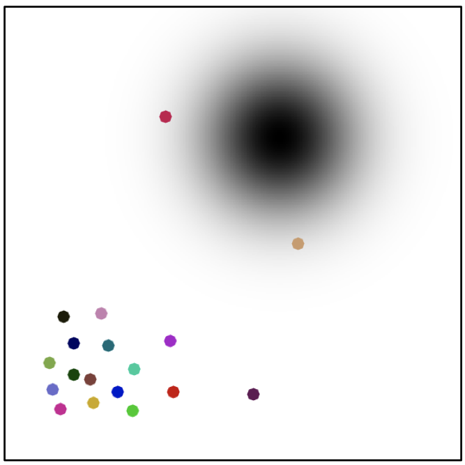
Refer to caption Refer to caption Refer to caption Refer to caption Refer to caption
α𝛼\alpha and β𝛽\beta =11\ell=1 =2020\ell=20 =4040\ell=40 =100100\ell=100
Figure 5.2: Iterations of the semidiscrete OT algorithm minimizing (5.8) (here a simple gradient descent is used). The support (yj)jsubscriptsubscript𝑦𝑗𝑗(y_{j})_{j} of the discrete measure β𝛽\beta is indicated by the colored points, while the continuous measure α𝛼\alpha is the uniform measure on a square. The colored cells display the Laguerre partition (𝕃j(g()))jsubscriptsubscript𝕃𝑗superscriptg𝑗(\mathbb{L}_{j}(\mathrm{\textbf{g}}^{(\ell)}))_{j} where g()superscriptg\mathrm{\textbf{g}}^{(\ell)} is the discrete dual potential computed at iteration \ell.

The initial idea of a semidiscrete solver for Monge–Ampère equations was proposed by Oliker and Prussner (1989), and its relation to the dual variational problem was shown by Aurenhammer et al. (1998). A theoretical analysis and its application to the reflector problem in optics is detailed in (Caffarelli et al., 1999). The semidiscrete formulation was used in (Carlier et al., 2010) in conjunction with a continuation approach based on Knothe’s transport. The recent revival of this methods in various fields is due to Mérigot (2011), who proposed a quasi-Newton solver and clarified the link with concepts from computational geometry. We refer to (Lévy and Schwindt, 2018) for a recent overview. The use of a Newton solver which is applied to sampling in computer graphics is proposed in (De Goes et al., 2012); see also (Lévy, 2015) for applications to 3-D volume and surface processing. An important area of application of the semidiscrete method is for the resolution of the incompressible fluid dynamic (Euler’s equations) using Lagrangian methods (de Goes et al., 2015; Gallouët and Mérigot, 2017). The semidiscrete OT solver enforces incompressibility at each iteration by imposing that the (possibly weighted) points cloud approximates a uniform distribution inside the domain. The convergence (with linear rate) of damped Newton iterations is proved in (Mirebeau, 2015) for the Monge–Ampère equation and is refined in (Kitagawa et al., 2016) for optimal transport. Semidiscrete OT finds important applications to illumination design, notably reflectors; see (Meyron et al., 2018).

5.3 Entropic Semidiscrete Formulation

The dual of the entropic regularized problem between arbitrary measures (4.9) is a smooth unconstrained optimization problem:

cε(α,β)=sup(f,g)𝒞(𝒳)×𝒞(𝒴)𝒳fdα+𝒴gdβε𝒳×𝒴ec+fgεdαdβ,superscriptsubscript𝑐𝜀𝛼𝛽𝑓𝑔𝒞𝒳𝒞𝒴supremumsubscript𝒳𝑓differential-d𝛼subscript𝒴𝑔differential-d𝛽𝜀subscript𝒳𝒴superscript𝑒direct-sum𝑐𝑓𝑔𝜀differential-d𝛼differential-d𝛽\mathcal{L}_{c}^{\varepsilon}(\alpha,\beta)=\underset{(f,g)\in\mathcal{C}(\mathcal{X})\times\mathcal{C}(\mathcal{Y})}{\sup}\;\int_{\mathcal{X}}f\mathrm{d}\alpha+\int_{\mathcal{Y}}g\mathrm{d}\beta-\varepsilon\int_{\mathcal{X}\times\mathcal{Y}}e^{\frac{-c+f\oplus g}{\varepsilon}}\mathrm{d}\alpha\mathrm{d}\beta, (5.9)

where we denoted (fg)(x,y)=def.f(x)+g(y)superscriptdef.direct-sum𝑓𝑔𝑥𝑦𝑓𝑥𝑔𝑦(f\oplus g)(x,y)\stackrel{{\scriptstyle\mbox{\tiny def.}}}{{=}}f(x)+g(y).

Similarly to the unregularized problem (5.1), one can minimize explicitly with respect to either f𝑓f or g𝑔g in (5.9), which yields a smoothed c𝑐c-transform

y𝒴,fc,ε(y)for-all𝑦𝒴superscript𝑓𝑐𝜀𝑦\displaystyle\forall\,y\in\mathcal{Y},\quad f^{c,\varepsilon}(y) =def.εlog(𝒳ec(x,y)+f(x)εdα(x)),superscriptdef.absent𝜀subscript𝒳superscript𝑒𝑐𝑥𝑦𝑓𝑥𝜀differential-d𝛼𝑥\displaystyle\stackrel{{\scriptstyle\mbox{\tiny def.}}}{{=}}-\varepsilon\log\left(\int_{\mathcal{X}}e^{\frac{-c(x,y)+f(x)}{\varepsilon}}\mathrm{d}\alpha(x)\right),
x𝒳,gc¯,ε(x)for-all𝑥𝒳superscript𝑔¯𝑐𝜀𝑥\displaystyle\forall\,x\in\mathcal{X},\quad g^{\bar{c},\varepsilon}(x) =def.εlog(𝒴ec(x,y)+g(y)εdβ(y)).superscriptdef.absent𝜀subscript𝒴superscript𝑒𝑐𝑥𝑦𝑔𝑦𝜀differential-d𝛽𝑦\displaystyle\stackrel{{\scriptstyle\mbox{\tiny def.}}}{{=}}-\varepsilon\log\left(\int_{\mathcal{Y}}e^{\frac{-c(x,y)+g(y)}{\varepsilon}}\mathrm{d}\beta(y)\right).

In the case of a discrete measure β=j=1mbjδyj𝛽superscriptsubscript𝑗1𝑚subscriptb𝑗subscript𝛿subscript𝑦𝑗\beta=\sum_{j=1}^{m}\mathrm{\textbf{b}}_{j}\delta_{y_{j}}, the problem simplifies as with (5.7) to a finite-dimensional problem expressed as a function of the discrete dual potential gmgsuperscript𝑚\mathrm{\textbf{g}}\in\mathbb{R}^{m},

x𝒳,gc¯,ε(x)=def.εlog(j=1mec(x,yj)+gjεbj).formulae-sequencefor-all𝑥𝒳superscriptdef.superscriptg¯𝑐𝜀𝑥𝜀superscriptsubscript𝑗1𝑚superscript𝑒𝑐𝑥subscript𝑦𝑗subscriptg𝑗𝜀subscriptb𝑗\forall\,x\in\mathcal{X},\quad\mathrm{\textbf{g}}^{\bar{c},\varepsilon}(x)\stackrel{{\scriptstyle\mbox{\tiny def.}}}{{=}}-\varepsilon\log\left(\sum_{j=1}^{m}e^{\frac{-c(x,y_{j})+\mathrm{\textbf{g}}_{j}}{\varepsilon}}\mathrm{\textbf{b}}_{j}\right). (5.10)

One defines similarly fc¯,εsuperscriptf¯𝑐𝜀\mathrm{\textbf{f}}^{\bar{c},\varepsilon} in the case of a discrete measure α𝛼\alpha. Note that the rewriting (4.40) and (4.41) of Sinkhorn using the soft-min operator minεsubscriptmin𝜀\text{min}_{\varepsilon}\, corresponds to the alternate computation of entropic smoothed c𝑐c-transforms,

fi(+1)=gc¯,ε(xi)andgj(+1)=fc,ε(yj).formulae-sequencesubscriptsuperscriptf1𝑖superscriptg¯𝑐𝜀subscript𝑥𝑖andsubscriptsuperscriptg1𝑗superscriptf𝑐𝜀subscript𝑦𝑗\mathrm{\textbf{f}}^{(\ell+1)}_{i}=\mathrm{\textbf{g}}^{\bar{c},\varepsilon}(x_{i})\quad\text{and}\quad\mathrm{\textbf{g}}^{(\ell+1)}_{j}=\mathrm{\textbf{f}}^{\,c,\varepsilon}(y_{j}). (5.11)

Instead of maximizing (5.9), one can thus solve the following finite-dimensional optimization problem:

maxgnε(g)=def.𝒳gc¯,ε(x)dα(x)+g,b.superscriptdef.gsuperscript𝑛superscript𝜀gsubscript𝒳superscriptg¯𝑐𝜀𝑥differential-d𝛼𝑥gb\underset{\mathrm{\textbf{g}}\in\mathbb{R}^{n}}{\max}\;\mathcal{E}^{\varepsilon}(\mathrm{\textbf{g}})\stackrel{{\scriptstyle\mbox{\tiny def.}}}{{=}}\int_{\mathcal{X}}\mathrm{\textbf{g}}^{\bar{c},\varepsilon}(x)\mathrm{d}\alpha(x)+\langle\mathrm{\textbf{g}},\,\mathrm{\textbf{b}}\rangle. (5.12)

Note that this optimization problem is still valid even in the unregularized case ε=0𝜀0\varepsilon=0 and in this case gc¯,ε=0=gc¯superscriptg¯𝑐𝜀0superscriptg¯𝑐\mathrm{\textbf{g}}^{\bar{c},\varepsilon=0}=\mathrm{\textbf{g}}^{\bar{c}} is the c¯¯𝑐\bar{c}-transform defined in (5.6) so that (5.12) is in fact (5.8). The gradient of this functional reads

jm,ε(g)j=𝒳χjε(x)dα(x)+bj,\forall\,j\in\llbracket m\rrbracket,\quad\nabla\mathcal{E}^{\varepsilon}(\mathrm{\textbf{g}})_{j}=-\int_{\mathcal{X}}\chi_{j}^{\varepsilon}(x)\mathrm{d}\alpha(x)+\mathrm{\textbf{b}}_{j}, (5.13)

where χjεsuperscriptsubscript𝜒𝑗𝜀\chi_{j}^{\varepsilon} is a smoothed version of the indicator χj0superscriptsubscript𝜒𝑗0\chi_{j}^{0} of the Laguerre cell 𝕃j(g)subscript𝕃𝑗g\mathbb{L}_{j}(\mathrm{\textbf{g}}),

χjε(x)=ec(x,yj)+gjεec(x,y)+gε.superscriptsubscript𝜒𝑗𝜀𝑥superscript𝑒𝑐𝑥subscript𝑦𝑗subscriptg𝑗𝜀subscriptsuperscript𝑒𝑐𝑥subscript𝑦subscriptg𝜀\chi_{j}^{\varepsilon}(x)=\frac{e^{\frac{-c(x,y_{j})+\mathrm{\textbf{g}}_{j}}{\varepsilon}}}{\sum_{\ell}e^{\frac{-c(x,y_{\ell})+\mathrm{\textbf{g}}_{\ell}}{\varepsilon}}}.

Note once again that this formula (5.13) is still valid for ε=0𝜀0\varepsilon=0. Note also that the family of functions (χjε)jsubscriptsuperscriptsubscript𝜒𝑗𝜀𝑗(\chi_{j}^{\varepsilon})_{j} is a partition of unity, i.e. jχjε=1subscript𝑗superscriptsubscript𝜒𝑗𝜀1\sum_{j}\chi_{j}^{\varepsilon}=1 and χjε0superscriptsubscript𝜒𝑗𝜀0\chi_{j}^{\varepsilon}\geq 0. Figure 5.3, bottom row, illustrates this.

Remark 5.1 (Second order methods and connection with logistic regression).

A crucial aspect of the smoothed semidiscrete formulation (5.12) is that it corresponds to the minimization of a smooth function. Indeed, as shown in (Genevay et al., 2016), the Hessian of εsuperscript𝜀\mathcal{E}^{\varepsilon} is upper bounded by 1/ε1𝜀1/\varepsilon, so that εsuperscript𝜀\nabla\mathcal{E}^{\varepsilon} is 1ε1𝜀\frac{1}{\varepsilon}-Lipschitz continuous. In fact, that problem is very closely related to a multiclass logistic regression problem (see Figure 5.3 for a display of the resulting fuzzy classification boundary) and enjoys the same favorable properties (see (Hosmer Jr et al., 2013)), which are generalizations of self-concordance; see (Bach, 2010). In particular, the Newton method converges quadratically, and one can use in practice quasi-Newton techniques, such as L-BFGS, as advocated in (Cuturi and Peyré, 2016). Note that (Cuturi and Peyré, 2016) studies the more general barycenter problem detailed in §9.2, but it is equivalent to this semidiscrete setting when considering only a pair of input measures. The use of second order schemes (Newton or L-BFGS) is also advocated in the unregularized case ε=0𝜀0\varepsilon=0 by (Mérigot, 2011; De Goes et al., 2012; Lévy, 2015). In (Kitagawa et al., 2016, Theo. 5.1), the Hessian of 0(g)superscript0g\mathcal{E}^{0}(\mathrm{\textbf{g}}) is shown to be uniformly bounded as long as the volume of the Laguerre cells is bounded by below and α𝛼\alpha has a continuous density. Kitagawa et al. proceed by showing the linear convergence of a damped Newton algorithm with a backtracking to ensure that the Laguerre cells never vanish between two iterations. This result justifies the use of second order methods even in the unregularized case. The intuition is that, while the conditioning of the entropic regularized problem scales like 1/ε1𝜀1/\varepsilon, when ε=0𝜀0\varepsilon=0, this conditioning is rather driven by m𝑚m, the number of samples of the discrete distribution (which controls the size of the Laguerre cells). Other methods exploiting second order schemes were also recently studied by (Knight and Ruiz, 2013; Sugiyama et al., 2017; Cohen et al., 2017; Allen-Zhu et al., 2017).
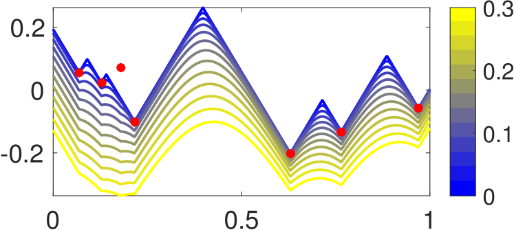
Refer to caption
Refer to caption Refer to caption Refer to caption Refer to caption
ε=0𝜀0\varepsilon=0 ε=0.01𝜀0.01\varepsilon=0.01 ε=0.1𝜀0.1\varepsilon=0.1 ε=0.3𝜀0.3\varepsilon=0.3
Figure 5.3: Top: examples of entropic semidiscrete c¯¯𝑐\bar{c}-transforms gc¯,εsuperscriptg¯𝑐𝜀\mathrm{\textbf{g}}^{\bar{c},\varepsilon} in one dimension, for ground cost c(x,y)=|xy|𝑐𝑥𝑦𝑥𝑦c(x,y)=|x-y| for varying ε𝜀\varepsilon (see colorbar). The red points are at locations (yj,gj)jsubscriptsubscript𝑦𝑗subscriptg𝑗𝑗(y_{j},-\mathrm{\textbf{g}}_{j})_{j}. Bottom: examples of entropic semidiscrete c¯¯𝑐\bar{c}-transforms gc¯,εsuperscriptg¯𝑐𝜀\mathrm{\textbf{g}}^{\bar{c},\varepsilon} in two dimensions, for ground cost c(x,y)=xy2𝑐𝑥𝑦subscriptnorm𝑥𝑦2c(x,y)=\left\|x-y\right\|_{2} for varying ε𝜀\varepsilon. The black curves are the level sets of the function gc¯,εsuperscriptg¯𝑐𝜀\mathrm{\textbf{g}}^{\bar{c},\varepsilon}, while the colors indicate the smoothed indicator function of the Laguerre cells χjεsuperscriptsubscript𝜒𝑗𝜀\chi_{j}^{\varepsilon}. The red points are at locations yj2subscript𝑦𝑗superscript2y_{j}\in\mathbb{R}^{2}, and their size is proportional to gjsubscriptg𝑗\mathrm{\textbf{g}}_{j}.
Remark 5.2 (Legendre transforms of OT cost functions).

As stated in Proposition 4.6, LCε(a,b)superscriptsubscriptLC𝜀ab\mathrm{L}_{\mathrm{\textbf{C}}}^{\varepsilon}(\mathrm{\textbf{a}},\mathrm{\textbf{b}}) is a convex function of (a,b)ab(\mathrm{\textbf{a}},\mathrm{\textbf{b}}) (which is also true in the unregularized case ε=0𝜀0\varepsilon=0). It is thus possible to compute its Legendre–Fenchel transform, which is defined in (4.54). Denoting Fa(b)=LCε(a,b)subscript𝐹absuperscriptsubscriptLC𝜀abF_{\mathrm{\textbf{a}}}(\mathrm{\textbf{b}})=\mathrm{L}_{\mathrm{\textbf{C}}}^{\varepsilon}(\mathrm{\textbf{a}},\mathrm{\textbf{b}}), one has, for a fixed a, following Cuturi and Peyré (2016):

Fa(g)=εH(a)+iaigc¯,ε(xi).superscriptsubscript𝐹ag𝜀𝐻asubscript𝑖subscripta𝑖superscriptg¯𝑐𝜀subscript𝑥𝑖F_{\mathrm{\textbf{a}}}^{*}(\mathrm{\textbf{g}})=-\varepsilon H(\mathrm{\textbf{a}})+\sum_{i}\mathrm{\textbf{a}}_{i}\mathrm{\textbf{g}}^{\bar{c},\varepsilon}(x_{i}).

Here gc¯,εsuperscriptg¯𝑐𝜀\mathrm{\textbf{g}}^{\bar{c},\varepsilon} is the entropic-smoothed c𝑐c-transform introduced in (5.10). In the unregularized case ε=0𝜀0\varepsilon=0, and for generic measures, Carlier et al. (2015) show, denoting α(β)=def.c(α,β)superscriptdef.subscript𝛼𝛽subscript𝑐𝛼𝛽\mathcal{F}_{\alpha}(\beta)\stackrel{{\scriptstyle\mbox{\tiny def.}}}{{=}}\mathcal{L}_{c}(\alpha,\beta),

g𝒞(𝒴),α(g)=𝒳gc¯(x)dα(x),formulae-sequencefor-all𝑔𝒞𝒴superscriptsubscript𝛼𝑔subscript𝒳superscript𝑔¯𝑐𝑥differential-d𝛼𝑥\forall\,g\in\mathcal{C}(\mathcal{Y}),\quad\mathcal{F}_{\alpha}^{*}(g)=\int_{\mathcal{X}}g^{\bar{c}}(x)\mathrm{d}\alpha(x),

where the c¯¯𝑐\bar{c}-transform gc¯𝒞(𝒳)superscript𝑔¯𝑐𝒞𝒳g^{\bar{c}}\in\mathcal{C}(\mathcal{X}) of g𝑔g is defined in §5.1. Note that here, since (𝒳)𝒳\mathcal{M}(\mathcal{X}) is in duality with 𝒞(𝒳)𝒞𝒳\mathcal{C}(\mathcal{X}), the Legendre transform is a function of continuous functions. Denoting now G(a,b)=def.LCε(a,b)superscriptdef.𝐺absuperscriptsubscriptLC𝜀abG(\mathrm{\textbf{a}},\mathrm{\textbf{b}})\stackrel{{\scriptstyle\mbox{\tiny def.}}}{{=}}\mathrm{L}_{\mathrm{\textbf{C}}}^{\varepsilon}(\mathrm{\textbf{a}},\mathrm{\textbf{b}}), one can derive as in (Cuturi and Peyré, 2016, 2018) the Legendre transform for both arguments,

(f,g)n×m,G(f,g)=εlogi,jeCi,j+fi+gjε,formulae-sequencefor-allfgsuperscript𝑛superscript𝑚superscript𝐺fg𝜀subscript𝑖𝑗superscript𝑒subscriptC𝑖𝑗subscriptf𝑖subscriptg𝑗𝜀\forall\,(\mathrm{\textbf{f}},\mathrm{\textbf{g}})\in\mathbb{R}^{n}\times\mathbb{R}^{m},\quad G^{*}(\mathrm{\textbf{f}},\mathrm{\textbf{g}})=-\varepsilon\log\sum_{i,j}e^{\frac{-\mathrm{\textbf{C}}_{i,j}+\mathrm{\textbf{f}}_{i}+\mathrm{\textbf{g}}_{j}}{\varepsilon}},

which can be seen as a smoothed version of the Legendre transform of 𝒢(α,β)=def.c(α,β)superscriptdef.𝒢𝛼𝛽subscript𝑐𝛼𝛽\mathcal{G}(\alpha,\beta)\stackrel{{\scriptstyle\mbox{\tiny def.}}}{{=}}\mathcal{L}_{c}(\alpha,\beta),

(f,g)𝒞(𝒳)×𝒞(𝒴),𝒢(f,g)=inf(x,y)𝒳×𝒴c(x,y)f(x)g(y).formulae-sequencefor-all𝑓𝑔𝒞𝒳𝒞𝒴superscript𝒢𝑓𝑔𝑥𝑦𝒳𝒴infimum𝑐𝑥𝑦𝑓𝑥𝑔𝑦\forall\,(f,g)\in\mathcal{C}(\mathcal{X})\times\mathcal{C}(\mathcal{Y}),\quad\mathcal{G}^{*}(f,g)=\underset{(x,y)\in\mathcal{X}\times\mathcal{Y}}{\inf}\;c(x,y)-f(x)-g(y).

5.4 Stochastic Optimization Methods

The semidiscrete formulation (5.8) and its smoothed version (5.12) are appealing because the energies to be minimized are written as an expectation with respect to the probability distribution α𝛼\alpha,

ε(g)=𝒳Eε(g,x)dα(x)=𝔼X(Eε(g,X))superscript𝜀gsubscript𝒳superscript𝐸𝜀g𝑥differential-d𝛼𝑥subscript𝔼𝑋superscript𝐸𝜀g𝑋\mathcal{E}^{\varepsilon}(\mathrm{\textbf{g}})=\int_{\mathcal{X}}E^{\varepsilon}(\mathrm{\textbf{g}},x)\mathrm{d}\alpha(x)=\mathbb{E}_{X}(E^{\varepsilon}(\mathrm{\textbf{g}},X))
whereEε(g,x)=def.gc¯,ε(x)g,b,superscriptdef.wheresuperscript𝐸𝜀g𝑥superscriptg¯𝑐𝜀𝑥gb\quad\text{where}\quad E^{\varepsilon}(\mathrm{\textbf{g}},x)\stackrel{{\scriptstyle\mbox{\tiny def.}}}{{=}}\mathrm{\textbf{g}}^{\bar{c},\varepsilon}(x)-\langle\mathrm{\textbf{g}},\,\mathrm{\textbf{b}}\rangle,

and X𝑋X denotes a random vector distributed on 𝒳𝒳\mathcal{X} according to α𝛼\alpha. Note that the gradient of each of the involved functional reads

gEε(x,g)=(χjε(x)bj)j=1mm.subscriptgsuperscript𝐸𝜀𝑥gsuperscriptsubscriptsuperscriptsubscript𝜒𝑗𝜀𝑥subscriptb𝑗𝑗1𝑚superscript𝑚\nabla_{\mathrm{\textbf{g}}}E^{\varepsilon}(x,\mathrm{\textbf{g}})=(\chi_{j}^{\varepsilon}(x)-\mathrm{\textbf{b}}_{j})_{j=1}^{m}\in\mathbb{R}^{m}.

One can thus use stochastic optimization methods to perform the maximization, as proposed in Genevay et al. (2016). This allows us to obtain provably convergent algorithms without the need to resort to an arbitrary discretization of α𝛼\alpha (either approximating α𝛼\alpha using sums of Diracs or using quadrature formula for the integrals). The measure α𝛼\alpha is used as a black box from which one can draw independent samples, which is a natural computational setup for many high-dimensional applications in statistics and machine learning. This class of methods has been generalized to the computation of Wasserstein barycenters (as described in §9.2) in (Staib et al., 2017b).

Stochastic gradient descent.

Initializing g(0)=𝟘Psuperscriptg0subscriptdouble-struck-𝟘𝑃\mathrm{\textbf{g}}^{(0)}=\mathbb{0}_{P}, the stochastic gradient descent algorithm (SGD; used here as a maximization method) draws at step \ell a point x𝒳subscript𝑥𝒳x_{\ell}\in\mathcal{X} according to distribution α𝛼\alpha (independently from all past and future samples (x)subscriptsubscript𝑥(x_{\ell})_{\ell}) to form the update

g(+1)=def.g()+τgEε(g(),x).superscriptdef.superscriptg1superscriptgsubscript𝜏subscriptgsuperscript𝐸𝜀superscriptgsubscript𝑥\mathrm{\textbf{g}}^{(\ell+1)}\stackrel{{\scriptstyle\mbox{\tiny def.}}}{{=}}\mathrm{\textbf{g}}^{(\ell)}+\tau_{\ell}\nabla_{\mathrm{\textbf{g}}}E^{\varepsilon}(\mathrm{\textbf{g}}^{(\ell)},x_{\ell}). (5.14)

The step size τsubscript𝜏\tau_{\ell} should decay fast enough to zero in order to ensure that the “noise” created by using gEε(x,g)subscriptgsuperscript𝐸𝜀subscript𝑥g\nabla_{\mathrm{\textbf{g}}}E^{\varepsilon}(x_{\ell},\mathrm{\textbf{g}}) as a proxy for the true gradient ε(g)superscript𝜀g\nabla\mathcal{E}^{\varepsilon}(\mathrm{\textbf{g}}) is canceled in the limit. A typical choice of schedule is

τ=def.τ01+/0,superscriptdef.subscript𝜏subscript𝜏01subscript0\tau_{\ell}\stackrel{{\scriptstyle\mbox{\tiny def.}}}{{=}}\frac{\tau_{0}}{1+\ell/\ell_{0}}, (5.15)

where 0subscript0\ell_{0} indicates roughly the number of iterations serving as a warmup phase. One can prove the convergence result

ε(g)𝔼(ε(g()))=O(1),superscript𝜀superscriptg𝔼superscript𝜀superscriptg𝑂1\mathcal{E}^{\varepsilon}(\mathrm{\textbf{g}}^{\star})-\mathbb{E}(\mathcal{E}^{\varepsilon}(\mathrm{\textbf{g}}^{(\ell)}))=O\left(\frac{1}{\sqrt{\ell}}\right),

where gsuperscriptg\mathrm{\textbf{g}}^{\star} is a solution of (5.12) and where 𝔼𝔼\mathbb{E} indicates an expectation with respect to the i.i.d. sampling of (x)subscriptsubscript𝑥(x_{\ell})_{\ell} performed at each iteration. Figure 5.4 shows the evolution of the algorithm on a simple 2-D example, where α𝛼\alpha is the uniform distribution on [0,1]2superscript012[0,1]^{2}.

Refer to caption
Figure 5.4: Evolution of the energy ε(g())superscript𝜀superscriptg\mathcal{E}^{\varepsilon}(\mathrm{\textbf{g}}^{(\ell)}), for ε=0𝜀0\varepsilon=0 (no regularization) during the SGD iterations (5.14). Each colored curve shows a different randomized run. The images display the evolution of the Laguerre cells (𝕃j(g()))jsubscriptsubscript𝕃𝑗superscriptg𝑗(\mathbb{L}_{j}(\mathrm{\textbf{g}}^{(\ell)}))_{j} through the iterations.
Stochastic gradient descent with averaging.

SGD is slow because of the fast decay of the stepsize τsubscript𝜏\tau_{\ell} toward zero. To improve the convergence speed, it is possible to average the past iterates, which is equivalent to running a “classical” SGD on auxiliary variables (g~())subscriptsuperscript~g(\tilde{\mathrm{\textbf{g}}}^{(\ell)})_{\ell}

g~(+1)=def.g~()+τgEε(g~(),x),superscriptdef.superscript~g1superscript~gsubscript𝜏subscriptgsuperscript𝐸𝜀superscript~gsubscript𝑥\tilde{\mathrm{\textbf{g}}}^{(\ell+1)}\stackrel{{\scriptstyle\mbox{\tiny def.}}}{{=}}\tilde{\mathrm{\textbf{g}}}^{(\ell)}+\tau_{\ell}\nabla_{\mathrm{\textbf{g}}}E^{\varepsilon}(\tilde{\mathrm{\textbf{g}}}^{(\ell)},x_{\ell}),

where xsubscript𝑥x_{\ell} is drawn according to α𝛼\alpha (and all the (x)subscriptsubscript𝑥(x_{\ell})_{\ell} are independent) and output as estimated weight vector the average

g()=def.1k=1g~(k).superscriptdef.superscriptg1superscriptsubscript𝑘1superscript~g𝑘\mathrm{\textbf{g}}^{(\ell)}\stackrel{{\scriptstyle\mbox{\tiny def.}}}{{=}}\frac{1}{\ell}\sum_{k=1}^{\ell}\tilde{\mathrm{\textbf{g}}}^{(k)}.

This defines the stochastic gradient descent with averaging (SGA) algorithm. Note that it is possible to avoid explicitly storing all the iterates by simply updating a running average as follows:

g(+1)=1+1g~(+1)++1g().superscriptg111superscript~g11superscriptg\mathrm{\textbf{g}}^{(\ell+1)}=\frac{1}{\ell+1}\tilde{\mathrm{\textbf{g}}}^{(\ell+1)}+\frac{\ell}{\ell+1}\mathrm{\textbf{g}}^{(\ell)}.

In this case, a typical choice of decay is rather of the form

τ=def.τ01+/0.superscriptdef.subscript𝜏subscript𝜏01subscript0\tau_{\ell}\stackrel{{\scriptstyle\mbox{\tiny def.}}}{{=}}\frac{\tau_{0}}{1+\sqrt{\ell/\ell_{0}}}.

Notice that the step size now goes much slower to 0 than for (5.15), at rate 1/2superscript12\ell^{-1/2}. Bach (2014) proves that SGA leads to a faster convergence (the constants involved are smaller) than SGD, since in contrast to SGD, SGA is adaptive to the local strong convexity (or concavity for maximization problems) of the functional.

Remark 5.3 (Continuous-continuous problems).

When neither α𝛼\alpha nor β𝛽\beta is a discrete measure, one cannot resort to semidiscrete strategies involving finite-dimensional dual variables, such as that given in Problem (5.7). The only option is to use stochastic optimization methods on the dual problem (4.45), as proposed in (Genevay et al., 2016). A suitable regularization of that problem is crucial, for instance by setting an entropic regularization strength ε>0𝜀0\varepsilon>0, to obtain an unconstrained problem that can be solved by stochastic descent schemes. A possible approach to revisit Problem (4.45) is to restrict that infinite-dimensional optimization problem over a space of continuous functions to a much smaller subset, such as that spanned by multilayer neural networks (Seguy et al., 2018). This approach leads to nonconvex finite-dimensional optimization problems with no approximation guarantees, but this can provide an effective way to compute a proxy for the Wasserstein distance in high-dimensional scenarios. Another solution is to use nonparametric families, which is equivalent to considering some sort of progressive refinement, as that proposed by Genevay et al. (2016) using reproducing kernel Hilbert spaces, whose dimension is proportional to the number of iterations of the SGD algorithm.

Chapter 6 𝒲1subscript𝒲1\operatorname{\mathcal{W}}_{1} Optimal Transport

This chapter focuses on optimal transport problems in which the ground cost is equal to a distance. Historically, this corresponds to the original problem posed by Monge in 1781; this setting was also that chosen in early applications of optimal transport in computer vision (Rubner et al., 2000) under the name of “earth mover’s distances”.

Unlike the case where the ground cost is a squared Hilbertian distance (studied in particular in Chapter 7), transport problems where the cost is a metric are more difficult to analyze theoretically. In contrast to Remark 2.24 that states the uniqueness of a transport map or coupling between two absolutely continuous measures when using a squared metric, the optimal Kantorovich coupling is in general not unique when the cost is the ground distance itself. Hence, in this regime it is often impossible to recover a uniquely defined Monge map, making this class of problems ill-suited for interpolation of measures. We refer to works by Trudinger and Wang (2001); Caffarelli et al. (2002); Sudakov (1979); Evans and Gangbo (1999) for proofs of existence of optimal 𝒲1subscript𝒲1\operatorname{\mathcal{W}}_{1} transportation plans and detailed analyses of their geometric structure.

Although more difficult to analyze in theory, optimal transport with a linear ground distance is usually more robust to outliers and noise than a quadratic cost. Furthermore, a cost that is a metric results in an elegant dual reformulation involving local flow, divergence constraints, or Lipschitzness of the dual potential, suggesting cheaper numerical algorithms that align with minimum-cost flow methods over networks in graph theory. This setting is also popular because the associated OT distances define a norm that can compare arbitrary distributions, even if they are not positive; this property is shared by a larger class of so-called dual norms (see §8.2 and Remark 6 for more details).

6.1 𝒲1subscript𝒲1\operatorname{\mathcal{W}}_{1} on Metric Spaces

Here we assume that d𝑑d is a distance on 𝒳=𝒴𝒳𝒴\mathcal{X}=\mathcal{Y}, and we solve the OT problem with the ground cost c(x,y)=d(x,y)𝑐𝑥𝑦𝑑𝑥𝑦c(x,y)=d(x,y). The following proposition highlights key properties of the c𝑐c-transform (5.1) in this setup. In the following, we denote the Lipschitz constant of a function f𝒞(𝒳)𝑓𝒞𝒳f\in\mathcal{C}(\mathcal{X}) as

Lip(f)=def.sup{|f(x)f(y)|d(x,y):(x,y)𝒳2,xy}.superscriptdef.Lip𝑓supremumconditional-set𝑓𝑥𝑓𝑦𝑑𝑥𝑦formulae-sequence𝑥𝑦superscript𝒳2𝑥𝑦\operatorname{Lip}(f)\stackrel{{\scriptstyle\mbox{\tiny def.}}}{{=}}\sup\left\{\frac{|f(x)-f(y)|}{d(x,y)}\;:\;(x,y)\in\mathcal{X}^{2},x\neq y\right\}.

We define Lipschitz functions to be those functions f𝑓f satisfying Lip(f)<+Lip𝑓\operatorname{Lip}(f)<+\infty; they form a convex subset of 𝒞(𝒳)𝒞𝒳\mathcal{C}(\mathcal{X}).

Proposition 6.1.

Suppose 𝒳=𝒴𝒳𝒴\mathcal{X}=\mathcal{Y} and c(x,y)=d(x,y)𝑐𝑥𝑦𝑑𝑥𝑦c(x,y)=d(x,y). Then, there exists g𝑔g such that f=gc𝑓superscript𝑔𝑐f=g^{c} if and only Lip(f)1Lip𝑓1\operatorname{Lip}(f)\leq 1. Furthermore, if Lip(f)1Lip𝑓1\operatorname{Lip}(f)\leq 1, then fc=fsuperscript𝑓𝑐𝑓f^{c}=-f.

Proof.

First, suppose f=gc𝑓superscript𝑔𝑐f=g^{c}. Then, for x,y𝒳𝑥𝑦𝒳x,y\in\mathcal{X},

|f(x)f(y)|𝑓𝑥𝑓𝑦\displaystyle|f(x)-f(y)| =|infz𝒳d(x,z)g(z)infz𝒳d(y,z)g(z)|absentsubscriptinfimum𝑧𝒳𝑑𝑥𝑧𝑔𝑧subscriptinfimum𝑧𝒳𝑑𝑦𝑧𝑔𝑧\displaystyle=\left|\inf_{z\in\mathcal{X}}d(x,z)-g(z)\;\;-\;\;\inf_{z\in\mathcal{X}}d(y,z)-g(z)\right|
supz𝒳|d(x,z)d(y,z)|d(x,y).absentsubscriptsupremum𝑧𝒳𝑑𝑥𝑧𝑑𝑦𝑧𝑑𝑥𝑦\displaystyle\leq\sup_{z\in\mathcal{X}}|d(x,z)-d(y,z)|\leq d(x,y).

The first equality follows from the definition of gcsuperscript𝑔𝑐g^{c}, the next inequality from the identity |inffinfg|sup|fg|infimum𝑓infimum𝑔supremum𝑓𝑔|\inf f-\inf g|\leq\sup|f-g|, and the last from the triangle inequality. This shows that Lip(f)1Lip𝑓1\operatorname{Lip}(f)\leq 1.

Now, suppose Lip(f)1Lip𝑓1\operatorname{Lip}(f)\leq 1, and define g=def.fsuperscriptdef.𝑔𝑓g\stackrel{{\scriptstyle\mbox{\tiny def.}}}{{=}}-f. By the Lipschitz property, for all x,y𝒳𝑥𝑦𝒳x,y\in\mathcal{X}, f(y)d(x,y)f(x)f(y)+d(x,y)𝑓𝑦𝑑𝑥𝑦𝑓𝑥𝑓𝑦𝑑𝑥𝑦f(y)-d(x,y)\leq f(x)\leq f(y)+d(x,y). Applying these inequalities,

gc(y)superscript𝑔𝑐𝑦\displaystyle g^{c}(y) =infx𝒳[d(x,y)+f(x)]infx𝒳[d(x,y)+f(y)d(x,y)]=f(y),absentsubscriptinfimum𝑥𝒳delimited-[]𝑑𝑥𝑦𝑓𝑥subscriptinfimum𝑥𝒳delimited-[]𝑑𝑥𝑦𝑓𝑦𝑑𝑥𝑦𝑓𝑦\displaystyle=\inf_{x\in\mathcal{X}}\left[d(x,y)+f(x)\right]\geq\inf_{x\in\mathcal{X}}\left[d(x,y)+f(y)-d(x,y)\right]=f(y),
gc(y)superscript𝑔𝑐𝑦\displaystyle g^{c}(y) =infx𝒳[d(x,y)+f(x)]infx𝒳[d(x,y)+f(y)+d(x,y)]=f(y).absentsubscriptinfimum𝑥𝒳delimited-[]𝑑𝑥𝑦𝑓𝑥subscriptinfimum𝑥𝒳delimited-[]𝑑𝑥𝑦𝑓𝑦𝑑𝑥𝑦𝑓𝑦\displaystyle=\inf_{x\in\mathcal{X}}\left[d(x,y)+f(x)\right]\leq\inf_{x\in\mathcal{X}}\left[d(x,y)+f(y)+d(x,y)\right]=f(y).

Hence, f=gc𝑓superscript𝑔𝑐f=g^{c} with g=f𝑔𝑓g=-f. Using the same inequalities shows

fc(y)superscript𝑓𝑐𝑦\displaystyle f^{c}(y) =infx𝒳[d(x,y)f(x)]infx𝒳[d(x,y)f(y)d(x,y)]=f(y),absentsubscriptinfimum𝑥𝒳delimited-[]𝑑𝑥𝑦𝑓𝑥subscriptinfimum𝑥𝒳delimited-[]𝑑𝑥𝑦𝑓𝑦𝑑𝑥𝑦𝑓𝑦\displaystyle=\inf_{x\in\mathcal{X}}\left[d(x,y)-f(x)\right]\geq\inf_{x\in\mathcal{X}}\left[d(x,y)-f(y)-d(x,y)\right]=-f(y),
fc(y)superscript𝑓𝑐𝑦\displaystyle f^{c}(y) =infx𝒳[d(x,y)f(x)]infx𝒳[d(x,y)f(y)+d(x,y)]=f(y).absentsubscriptinfimum𝑥𝒳delimited-[]𝑑𝑥𝑦𝑓𝑥subscriptinfimum𝑥𝒳delimited-[]𝑑𝑥𝑦𝑓𝑦𝑑𝑥𝑦𝑓𝑦\displaystyle=\inf_{x\in\mathcal{X}}\left[d(x,y)-f(x)\right]\leq\inf_{x\in\mathcal{X}}\left[d(x,y)-f(y)+d(x,y)\right]=-f(y).

This shows fc=fsuperscript𝑓𝑐𝑓f^{c}=-f. ∎

Starting from the single potential formulation (5.4), one can iterate the construction and replace the couple (g,gc)𝑔superscript𝑔𝑐(g,g^{c}) by (gc,(gc)c)superscript𝑔𝑐superscriptsuperscript𝑔𝑐𝑐(g^{c},(g^{c})^{c}). The last proposition shows that one can thus use (gc,gc)superscript𝑔𝑐superscript𝑔𝑐(g^{c},-g^{c}), which in turn is equivalent to any pair (f,f)𝑓𝑓(f,-f) such that Lip(f)1Lip𝑓1\operatorname{Lip}(f)\leq 1. This leads to the following alternative expression for the 𝒲1subscript𝒲1\operatorname{\mathcal{W}}_{1} distance:

𝒲1(α,β)=max𝑓{𝒳f(x)(dα(x)dβ(x)):Lip(f)1}.subscript𝒲1𝛼𝛽𝑓conditional-setsubscript𝒳𝑓𝑥d𝛼𝑥d𝛽𝑥Lip𝑓1\operatorname{\mathcal{W}}_{1}(\alpha,\beta)=\underset{f}{\max}\;\left\{\int_{\mathcal{X}}f(x)(\mathrm{d}\alpha(x)-\mathrm{d}\beta(x))\;:\;\operatorname{Lip}(f)\leq 1\right\}. (6.1)

This expression shows that 𝒲1subscript𝒲1\operatorname{\mathcal{W}}_{1} is actually a norm, i.e. 𝒲1(α,β)=αβ𝒲1subscript𝒲1𝛼𝛽subscriptnorm𝛼𝛽subscript𝒲1\operatorname{\mathcal{W}}_{1}(\alpha,\beta)=\left\|\alpha-\beta\right\|_{\operatorname{\mathcal{W}}_{1}}, and that it is still valid for any measures (not necessary positive) as long as 𝒳α=𝒳βsubscript𝒳𝛼subscript𝒳𝛽\int_{\mathcal{X}}\alpha=\int_{\mathcal{X}}\beta. This norm is often called the Kantorovich and Rubinstein norm (1958).

For discrete measures of the form (2.1), writing αβ=kmkδzk𝛼𝛽subscript𝑘subscriptm𝑘subscript𝛿subscript𝑧𝑘\alpha-\beta=\sum_{k}\mathrm{\textbf{m}}_{k}\delta_{z_{k}} with zk𝒳subscript𝑧𝑘𝒳z_{k}\in\mathcal{X} and kmk=0subscript𝑘subscriptm𝑘0\sum_{k}\mathrm{\textbf{m}}_{k}=0, the optimization (6.1) can be rewritten as

𝒲1(α,β)=max(fk)k{kfkmk:(k,),|fkf|d(zk,z),}\operatorname{\mathcal{W}}_{1}(\alpha,\beta)=\underset{(\mathrm{\textbf{f}}_{k})_{k}}{\max}\;\left\{\sum_{k}\mathrm{\textbf{f}}_{k}\mathrm{\textbf{m}}_{k}\;:\;\forall\,(k,\ell),\left\lvert\mathrm{\textbf{f}}_{k}-\mathrm{\textbf{f}}_{\ell}\right\rvert\leq d(z_{k},z_{\ell}),\right\} (6.2)

which is a finite-dimensional convex program with quadratic-cone constraints. It can be solved using interior point methods or, as we detail next for a similar problem, using proximal methods.

When using d(x,y)=|xy|𝑑𝑥𝑦𝑥𝑦d(x,y)=|x-y| with 𝒳=𝒳\mathcal{X}=\mathbb{R}, we can reduce the number of constraints by ordering the zksubscript𝑧𝑘z_{k}’s via z1z2subscript𝑧1subscript𝑧2z_{1}\leq z_{2}\leq\ldots. In this case, we only have to solve

𝒲1(α,β)=max(fk)k{kfkmk:k,|fk+1fk|zk+1zk},subscript𝒲1𝛼𝛽subscriptsubscriptf𝑘𝑘conditional-setsubscript𝑘subscriptf𝑘subscriptm𝑘for-all𝑘subscriptf𝑘1subscriptf𝑘subscript𝑧𝑘1subscript𝑧𝑘\operatorname{\mathcal{W}}_{1}(\alpha,\beta)=\underset{(\mathrm{\textbf{f}}_{k})_{k}}{\max}\;\left\{\sum_{k}\mathrm{\textbf{f}}_{k}\mathrm{\textbf{m}}_{k}\;:\;\forall\,k,\left\lvert\mathrm{\textbf{f}}_{k+1}-\mathrm{\textbf{f}}_{k}\right\rvert\leq z_{k+1}-z_{k}\right\},

which is a linear program. Note that furthermore, in this 1-D case, a closed form expression for 𝒲1subscript𝒲1\operatorname{\mathcal{W}}_{1} using cumulative functions is given in (2.37).

Remark 6.1 (𝒲psubscript𝒲𝑝\operatorname{\mathcal{W}}_{p} with 0<p10𝑝10<p\leq 1).

If 0<p10𝑝10<p\leq 1, then d~(x,y)=def.d(x,y)psuperscriptdef.~𝑑𝑥𝑦𝑑superscript𝑥𝑦𝑝\tilde{d}(x,y)\stackrel{{\scriptstyle\mbox{\tiny def.}}}{{=}}d(x,y)^{p} satisfies the triangular inequality, and hence d~~𝑑\tilde{d} is itself a distance. One can thus apply the results and algorithms detailed above for 𝒲1subscript𝒲1\operatorname{\mathcal{W}}_{1} to compute 𝒲psubscript𝒲𝑝\operatorname{\mathcal{W}}_{p} by simply using d~~𝑑\tilde{d} in place of d𝑑d. This is equivalent to stating that 𝒲psubscript𝒲𝑝\operatorname{\mathcal{W}}_{p} is the dual of p𝑝p-Hölder functions {f:Lipp(f)1}conditional-set𝑓subscriptLip𝑝𝑓1\{f\;:\;\operatorname{Lip}_{p}(f)\leq 1\}, where

Lipp(f)=def.sup{|f(x)f(y)|d(x,y)p:(x,y)𝒳2,xy}.superscriptdef.subscriptLip𝑝𝑓supremumconditional-set𝑓𝑥𝑓𝑦𝑑superscript𝑥𝑦𝑝formulae-sequence𝑥𝑦superscript𝒳2𝑥𝑦\operatorname{Lip}_{p}(f)\stackrel{{\scriptstyle\mbox{\tiny def.}}}{{=}}\sup\left\{\frac{|f(x)-f(y)|}{d(x,y)^{p}}\;:\;(x,y)\in\mathcal{X}^{2},x\neq y\right\}.

6.2 𝒲1subscript𝒲1\operatorname{\mathcal{W}}_{1} on Euclidean Spaces

In the special case of Euclidean spaces 𝒳=𝒴=d𝒳𝒴superscript𝑑\mathcal{X}=\mathcal{Y}=\mathbb{R}^{d}, using c(x,y)=xy𝑐𝑥𝑦norm𝑥𝑦c(x,y)=\left\|x-y\right\|, the global Lipschitz constraint appearing in (6.1) can be made local as a uniform bound on the gradient of f𝑓f,

𝒲1(α,β)=max𝑓{df(x)(dα(x)dβ(x)):f1}.subscript𝒲1𝛼𝛽𝑓conditional-setsubscriptsuperscript𝑑𝑓𝑥d𝛼𝑥d𝛽𝑥subscriptnorm𝑓1\operatorname{\mathcal{W}}_{1}(\alpha,\beta)=\underset{f}{\max}\;\left\{\int_{\mathbb{R}^{d}}f(x)(\mathrm{d}\alpha(x)-\mathrm{d}\beta(x))\;:\;\left\|\nabla f\right\|_{\infty}\leq 1\right\}. (6.3)

Here the constraint f1subscriptnorm𝑓1\left\|\nabla f\right\|_{\infty}\leq 1 signifies that the norm of the gradient of f𝑓f at any point x𝑥x is upper bounded by 111, f(x)21subscriptnorm𝑓𝑥21\left\|\nabla f(x)\right\|_{2}\leq 1 for any x𝑥x.

Considering the dual problem to (6.3), one obtains an optimization problem under fixed divergence constraint

𝒲1(α,β)=min𝑠{ds(x)2dx:div(s)=αβ},subscript𝒲1𝛼𝛽𝑠conditional-setsubscriptsuperscript𝑑:evaluated-at𝑠𝑥2d𝑥div𝑠𝛼𝛽\operatorname{\mathcal{W}}_{1}(\alpha,\beta)=\underset{s}{\min}\;\left\{\int_{\mathbb{R}^{d}}\left\|s(x)\right\|_{2}\mathrm{d}x\;:\;\operatorname{div}(s)=\alpha-\beta\right\}, (6.4)

which is often called the Beckmann formulation (Beckmann, 1952). Here the vectorial function s(x)2𝑠𝑥superscript2s(x)\in\mathbb{R}^{2} can be interpreted as a flow field, describing locally the movement of mass. Outside the support of the two input measures, div(s)=0div𝑠0\operatorname{div}(s)=0, which is the conservation of mass constraint. Once properly discretized using finite elements, Problems (6.3) and (6.4) become nonsmooth convex optimization problems. It is possible to use an off-the-shelf interior points quadratic-cone optimization solver, but as advocated in §7.3, large-scale problems require the use of simpler but more adapted first order methods. One can thus use, for instance, Douglas–Rachford (DR) iterations (7.14) or the related alternating direction method of multipliers method. Note that on a uniform grid, projecting on the divergence constraint is conveniently handled using the fast Fourier transform. We refer to Solomon et al. (2014a) for a detailed account for these approaches and application to OT on triangulated meshes. See also Li et al. (2018a); Ryu et al. (2017b, a) for similar approaches using primal-dual splitting schemes. Approximation schemes that relax the Lipschitz constraint on the dual potentials f𝑓f have also been proposed, using, for instance, a constraint on wavelet coefficients leading to an explicit formula (Shirdhonkar and Jacobs, 2008), or by considering only functions f𝑓f parameterized as multilayer neural networks with “rectified linear” max(0,)0\max(0,\cdot) activation function and clipped weights (Arjovsky et al., 2017).

6.3 𝒲1subscript𝒲1\operatorname{\mathcal{W}}_{1} on a Graph

The previous formulations (6.3) and (6.4) of 𝒲1subscript𝒲1\operatorname{\mathcal{W}}_{1} can be generalized to the setting where 𝒳𝒳\mathcal{X} is a geodesic space, i.e. c(x,y)=d(x,y)𝑐𝑥𝑦𝑑𝑥𝑦c(x,y)=d(x,y) where d𝑑d is a geodesic distance. We refer to Feldman and McCann (2002) for a theoretical analysis in the case where 𝒳𝒳\mathcal{X} is a Riemannian manifold. When 𝒳=1,n𝒳1𝑛\mathcal{X}=\llbracket 1,n\rrbracket is a discrete set, equipped with undirected edges (i,j)𝒳2𝑖𝑗superscript𝒳2(i,j)\in\mathcal{E}\subset\mathcal{X}^{2} labeled with a weight (length) wi,jsubscriptw𝑖𝑗\mathrm{\textbf{w}}_{i,j}, we recover the important case where 𝒳𝒳\mathcal{X} is a graph equipped with the geodesic distance (or shortest path metric):

Di,j=def.minK0,(ik)k:ij{k=1K1wik,ik+1:k1,K1,(ik,ik+1)},superscriptdef.subscriptD𝑖𝑗:𝐾0subscriptsubscript𝑖𝑘𝑘𝑖𝑗conditional-setsuperscriptsubscript𝑘1𝐾1subscriptwsubscript𝑖𝑘subscript𝑖𝑘1formulae-sequencefor-all𝑘1𝐾1subscript𝑖𝑘subscript𝑖𝑘1\mathrm{\textbf{D}}_{i,j}\stackrel{{\scriptstyle\mbox{\tiny def.}}}{{=}}\underset{K\geq 0,(i_{k})_{k}:i\rightarrow j}{\min}\;\left\{\sum_{k=1}^{K-1}\mathrm{\textbf{w}}_{i_{k},i_{k+1}}\;:\;\forall\,k\in\llbracket 1,K-1\rrbracket,(i_{k},i_{k+1})\in\mathcal{E}\right\},

where ij𝑖𝑗i\rightarrow j indicates that i1=isubscript𝑖1𝑖i_{1}=i and iK=jsubscript𝑖𝐾𝑗i_{K}=j, namely that the path starts at i𝑖i and ends at j𝑗j.

We consider two vectors (a,b)(n)2absuperscriptsuperscript𝑛2(\mathrm{\textbf{a}},\mathrm{\textbf{b}})\in(\mathbb{R}^{n})^{2} defining (signed) discrete measures on the graph 𝒳𝒳\mathcal{X} such that iai=ibisubscript𝑖subscripta𝑖subscript𝑖subscriptb𝑖\sum_{i}\mathrm{\textbf{a}}_{i}=\sum_{i}\mathrm{\textbf{b}}_{i} (these weights do not need to be positive). The goal is now to compute W1(a,b)subscriptW1ab\operatorname{\mathrm{W}}_{1}(\mathrm{\textbf{a}},\mathrm{\textbf{b}}), as introduced in (2.17) for p=1𝑝1p=1, when the ground metric is the graph geodesic distance. This computation should be carried out without going as far as having to compute a “full” coupling P of size n×n𝑛𝑛n\times n, to rely instead on local operators thanks to the underlying connectivity of the graph. These operators are discrete formulations for the gradient and divergence differential operators.

A discrete dual Kantorovich potential fnfsuperscript𝑛\mathrm{\textbf{f}}\in\mathbb{R}^{n} is a vector indexed by all vertices of the graph. The gradient operator :n:superscript𝑛superscript\nabla:\mathbb{R}^{n}\rightarrow\mathbb{R}^{\mathcal{E}} is defined as

(i,j),(f)i,j=def.fifj.formulae-sequencefor-all𝑖𝑗superscriptdef.subscriptf𝑖𝑗subscriptf𝑖subscriptf𝑗\forall\,(i,j)\in\mathcal{E},\quad(\nabla\mathrm{\textbf{f}})_{i,j}\stackrel{{\scriptstyle\mbox{\tiny def.}}}{{=}}\mathrm{\textbf{f}}_{i}-\mathrm{\textbf{f}}_{j}.

A flow s=(si,j)i,jssubscriptsubscripts𝑖𝑗𝑖𝑗\mathrm{\textbf{s}}=(\mathrm{\textbf{s}}_{i,j})_{i,j} is defined on edges, and the divergence operator div:n:divsuperscriptsuperscript𝑛\operatorname{div}:\mathbb{R}^{\mathcal{E}}\rightarrow\mathbb{R}^{n}, which is the adjoint of the gradient \nabla, maps flows to vectors defined on vertices and is defined as

i1,n,div(s)i=def.j:(i,j)(si,jsj,i)n.\forall\,i\in\llbracket 1,n\rrbracket,\quad\operatorname{div}(\mathrm{\textbf{s}})_{i}\stackrel{{\scriptstyle\mbox{\tiny def.}}}{{=}}\sum_{j:(i,j)\in\mathcal{E}}(\mathrm{\textbf{s}}_{i,j}-\mathrm{\textbf{s}}_{j,i})\in\mathbb{R}^{n}.

Problem (6.3) becomes, in the graph setting,

W1(a,b)=maxfn{i=1nfi(aibi):(i,j),|(f)i,j|wi,j}.subscriptW1abfsuperscript𝑛conditional-setsuperscriptsubscript𝑖1𝑛subscriptf𝑖subscripta𝑖subscriptb𝑖formulae-sequencefor-all𝑖𝑗subscriptf𝑖𝑗subscriptw𝑖𝑗\operatorname{\mathrm{W}}_{1}(\mathrm{\textbf{a}},\mathrm{\textbf{b}})=\underset{\mathrm{\textbf{f}}\in\mathbb{R}^{n}}{\max}\;\left\{\sum_{i=1}^{n}\mathrm{\textbf{f}}_{i}(\mathrm{\textbf{a}}_{i}-\mathrm{\textbf{b}}_{i})\;:\;\forall(i,j)\in\mathcal{E},\,|(\nabla\mathrm{\textbf{f}})_{i,j}|\leq\mathrm{\textbf{w}}_{i,j}\right\}. (6.5)

The associated dual problem, which is analogous to Formula (6.4), is then

W1(a,b)=mins+{(i,j)wi,jsi,j:div(s)=ab}.subscriptW1abssuperscriptsubscriptconditional-setsubscript𝑖𝑗subscriptw𝑖𝑗subscripts𝑖𝑗divsab\operatorname{\mathrm{W}}_{1}(\mathrm{\textbf{a}},\mathrm{\textbf{b}})=\underset{\mathrm{\textbf{s}}\in\mathbb{R}_{+}^{\mathcal{E}}}{\min}\;\left\{\sum_{(i,j)\in\mathcal{E}}\mathrm{\textbf{w}}_{i,j}\mathrm{\textbf{s}}_{i,j}\;:\;\operatorname{div}(\mathrm{\textbf{s}})=\mathrm{\textbf{a}}-\mathrm{\textbf{b}}\right\}. (6.6)

This is a linear program and more precisely an instance of min-cost flow problems. Highly efficient dedicated simplex solvers have been devised to solve it; see, for instance, (Ling and Okada, 2007). Figure 6.1 shows an example of primal and dual solutions. Formulation (6.6) is the so-called Beckmann formulation (Beckmann, 1952) and has been used and extended to define and study traffic congestion models; see, for instance, (Carlier et al., 2008).
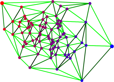
Refer to caption Refer to caption
f (a,b)ab({\color[rgb]{1,0,0}\mathrm{\textbf{a}}},{\color[rgb]{0,0,1}\mathrm{\textbf{b}}}) and s
Figure 6.1: Example of computation of W1(a,b)subscriptW1ab\operatorname{\mathrm{W}}_{1}(\mathrm{\textbf{a}},\mathrm{\textbf{b}}) on a planar graph with uniform weights wi,j=1subscriptw𝑖𝑗1\mathrm{\textbf{w}}_{i,j}=1. Left: potential f solution of (6.5) (increasing value from red to blue). The green color of the edges is proportional to |(f)i,j|subscriptf𝑖𝑗|(\nabla\mathrm{\textbf{f}})_{i,j}|. Right: flow s solution of (6.6), where bold black edges display nonzero si,jsubscripts𝑖𝑗\mathrm{\textbf{s}}_{i,j}, which saturate to wi,j=1subscriptw𝑖𝑗1\mathrm{\textbf{w}}_{i,j}=1. These saturating flow edge on the right match the light green edge on the left where |(f)i,j|=1subscriptf𝑖𝑗1|(\nabla\mathrm{\textbf{f}})_{i,j}|=1.

Chapter 7 Dynamic Formulations

This chapter presents the geodesic (also called dynamic) point of view of optimal transport when the cost is a squared geodesic distance. This describes the optimal transport between two measures as a curve in the space of measures minimizing a total length. The dynamic point of view offers an alternative and intuitive interpretation of optimal transport, which not only allows us to draw links with fluid dynamics but also results in an efficient numerical tool to compute OT in small dimensions when interpolating between two densities. The drawback of that approach is that it cannot scale to large-scale sparse measures and works only in low dimensions on regular domains (because one needs to grid the space) with a squared geodesic cost.

In this chapter, we use the notation (α0,α1)subscript𝛼0subscript𝛼1(\alpha_{0},\alpha_{1}) in place of (α,β)𝛼𝛽(\alpha,\beta) in agreement with the idea that we start at time t=0𝑡0t=0 from one measure to reach another one at time t=1𝑡1t=1.

7.1 Continuous Formulation

In the case 𝒳=𝒴=d𝒳𝒴superscript𝑑\mathcal{X}=\mathcal{Y}=\mathbb{R}^{d}, and c(x,y)=xy2𝑐𝑥𝑦superscriptnorm𝑥𝑦2c(x,y)=\left\|x-y\right\|^{2}, the optimal transport distance 𝒲22(α,β)=c(α,β)superscriptsubscript𝒲22𝛼𝛽subscript𝑐𝛼𝛽\operatorname{\mathcal{W}}_{2}^{2}(\alpha,\beta)=\mathcal{L}_{c}(\alpha,\beta) as defined in (2.15) can be computed by looking for a minimal length path (αt)t=01superscriptsubscriptsubscript𝛼𝑡𝑡01(\alpha_{t})_{t=0}^{1} between these two measures. This path is described by advecting the measure using a vector field vtsubscript𝑣𝑡v_{t} defined at each instant. The vector field vtsubscript𝑣𝑡v_{t} and the path αtsubscript𝛼𝑡\alpha_{t} must satisfy the conservation of mass formula, resulting in

αtt+div(αtvt)=0andαt=0=α0,αt=1=α1,formulae-sequencesubscript𝛼𝑡𝑡divsubscript𝛼𝑡subscript𝑣𝑡0andformulae-sequencesubscript𝛼𝑡0subscript𝛼0subscript𝛼𝑡1subscript𝛼1\frac{\partial\alpha_{t}}{\partial t}+\operatorname{div}(\alpha_{t}v_{t})=0\quad\text{and}\quad\alpha_{t=0}=\alpha_{0},\alpha_{t=1}=\alpha_{1}, (7.1)

where the equation above should be understood in the sense of distributions on dsuperscript𝑑\mathbb{R}^{d}. The infinitesimal length of such a vector field is measured using the L2superscript𝐿2L^{2} norm associated to the measure αtsubscript𝛼𝑡\alpha_{t}, that is defined as

vtL2(αt)=(dvt(x)2dαt(x))1/2.subscriptnormsubscript𝑣𝑡superscript𝐿2subscript𝛼𝑡superscriptsubscriptsuperscript𝑑superscriptnormsubscript𝑣𝑡𝑥2differential-dsubscript𝛼𝑡𝑥12\left\|v_{t}\right\|_{L^{2}(\alpha_{t})}=\left(\int_{\mathbb{R}^{d}}\left\|v_{t}(x)\right\|^{2}\mathrm{d}\alpha_{t}(x)\right)^{1/2}.

This definition leads to the following minimal-path reformulation of 𝒲2subscript𝒲2\operatorname{\mathcal{W}}_{2}, originally introduced by Benamou and Brenier (2000):

𝒲22(α0,α1)=min(αt,vt)t sat. (7.1)01dvt(x)2dαt(x)dt,superscriptsubscript𝒲22subscript𝛼0subscript𝛼1subscriptsubscript𝛼𝑡subscript𝑣𝑡𝑡 sat. (7.1)superscriptsubscript01subscriptsuperscript𝑑superscriptnormsubscript𝑣𝑡𝑥2differential-dsubscript𝛼𝑡𝑥differential-d𝑡\operatorname{\mathcal{W}}_{2}^{2}(\alpha_{0},\alpha_{1})=\underset{(\alpha_{t},v_{t})_{t}\text{ sat. \eqref{eq-cons-bb-ncvx}}}{\min}\;\int_{0}^{1}\int_{\mathbb{R}^{d}}\left\|v_{t}(x)\right\|^{2}\mathrm{d}\alpha_{t}(x)\mathrm{d}t, (7.2)

where αtsubscript𝛼𝑡\alpha_{t} is a scalar-valued measure and vtsubscript𝑣𝑡v_{t} a vector-valued measure. Figure 7.1 shows two examples of such paths of measures.

Refer to caption Refer to caption Refer to caption Refer to caption Refer to caption
α0subscript𝛼0\alpha_{0} α1/4subscript𝛼14\alpha_{1/4} α1/2subscript𝛼12\alpha_{1/2} α3/4subscript𝛼34\alpha_{3/4} α1subscript𝛼1\alpha_{1}
Figure 7.1: Displacement interpolation αtsubscript𝛼𝑡\alpha_{t} satisfying (7.2). Top: for two measures (α0,α1)subscript𝛼0subscript𝛼1(\alpha_{0},\alpha_{1}) with densities with respect to the Lebesgue measure. Bottom: for two discrete empirical measures with the same number of points (bottom).

The formulation (7.2) is a nonconvex formulation in the variables (αt,vt)tsubscriptsubscript𝛼𝑡subscript𝑣𝑡𝑡(\alpha_{t},v_{t})_{t} because of the constraint (7.1) involving the product αtvtsubscript𝛼𝑡subscript𝑣𝑡\alpha_{t}v_{t}. Introducing a vector-valued measure (often called the “momentum”)

Jt=def.αtvt,superscriptdef.subscript𝐽𝑡subscript𝛼𝑡subscript𝑣𝑡J_{t}\stackrel{{\scriptstyle\mbox{\tiny def.}}}{{=}}\alpha_{t}v_{t},

Benamou and Brenier showed in their landmark paper (2000) that it is instead convex in the variable (αt,Jt)tsubscriptsubscript𝛼𝑡subscript𝐽𝑡𝑡(\alpha_{t},J_{t})_{t} when writing

𝒲22(α0,α1)=min(αt,Jt)t𝒞(α0,α1)01dθ(αt(x),Jt(x))dxdt,superscriptsubscript𝒲22subscript𝛼0subscript𝛼1subscriptsubscript𝛼𝑡subscript𝐽𝑡𝑡𝒞subscript𝛼0subscript𝛼1superscriptsubscript01subscriptsuperscript𝑑𝜃subscript𝛼𝑡𝑥subscript𝐽𝑡𝑥differential-d𝑥differential-d𝑡\operatorname{\mathcal{W}}_{2}^{2}(\alpha_{0},\alpha_{1})=\underset{(\alpha_{t},J_{t})_{t}\in\mathcal{C}(\alpha_{0},\alpha_{1})}{\min}\;\int_{0}^{1}\int_{\mathbb{R}^{d}}\theta(\alpha_{t}(x),J_{t}(x))\mathrm{d}x\mathrm{d}t, (7.3)

where we define the set of constraints as

𝒞(α0,α1)=def.{(αt,Jt):αtt+div(Jt)=0,αt=0=α0,αt=1=α1},superscriptdef.𝒞subscript𝛼0subscript𝛼1conditional-setsubscript𝛼𝑡subscript𝐽𝑡formulae-sequencesubscript𝛼𝑡𝑡divsubscript𝐽𝑡0formulae-sequencesubscript𝛼𝑡0subscript𝛼0subscript𝛼𝑡1subscript𝛼1\mathcal{C}(\alpha_{0},\alpha_{1})\stackrel{{\scriptstyle\mbox{\tiny def.}}}{{=}}\left\{(\alpha_{t},J_{t})\;:\;\frac{\partial\alpha_{t}}{\partial t}+\operatorname{div}(J_{t})=0,\alpha_{t=0}=\alpha_{0},\alpha_{t=1}=\alpha_{1}\right\}, (7.4)

and where θ:+{+}\theta:\rightarrow\mathbb{R}^{+}\cup\{+\infty\} is the following lower semicontinuous convex function

(a,b)+×d,θ(a,b)={b2aifa>0,0if(a,b)=0,+otherwise.formulae-sequencefor-all𝑎𝑏subscriptsuperscript𝑑𝜃𝑎𝑏casessuperscriptnorm𝑏2𝑎if𝑎00if𝑎𝑏0otherwise\forall\,(a,b)\in\mathbb{R}_{+}\times\mathbb{R}^{d},\quad\theta(a,b)=\left\{\begin{array}[]{l}\frac{\left\|b\right\|^{2}}{a}\quad\text{if}\quad a>0,\\ 0\quad\text{if}\quad(a,b)=0,\\ +\infty\quad\text{otherwise}.\end{array}\right. (7.5)

This definition might seem complicated, but it is crucial to impose that the momentum Jt(x)subscript𝐽𝑡𝑥J_{t}(x) should vanish when αt(x)=0subscript𝛼𝑡𝑥0\alpha_{t}(x)=0. Note also that (7.3) is written in an informal way as if the measures (αt,Jt)subscript𝛼𝑡subscript𝐽𝑡(\alpha_{t},J_{t}) were density functions, but this is acceptable because θ𝜃\theta is a 1-homogeneous function (and hence defined even if the measures do not have a density with respect to Lebesgue measure) and can thus be extended in an unambiguous way from density to functions.

Remark 7.1 (Links with McCann’s interpolation).
In the case (see Equation (2.28)) where there exists an optimal Monge map T:dd:𝑇superscript𝑑superscript𝑑T:\mathbb{R}^{d}\rightarrow\mathbb{R}^{d} with Tα0=α1subscript𝑇subscript𝛼0subscript𝛼1T_{\sharp}\alpha_{0}=\alpha_{1}, then αtsubscript𝛼𝑡\alpha_{t} is equal to McCann’s interpolation αt=((1t)Id+tT)α0.subscript𝛼𝑡subscript1𝑡Id𝑡𝑇subscript𝛼0\alpha_{t}=((1-t)\mathrm{Id}+tT)_{\sharp}\alpha_{0}. (7.6) In the 1-D case, using Remark 2.30, this interpolation can be computed thanks to the relation 𝒞αt1=(1t)𝒞α01+t𝒞α11;superscriptsubscript𝒞subscript𝛼𝑡11𝑡superscriptsubscript𝒞subscript𝛼01𝑡superscriptsubscript𝒞subscript𝛼11\mathcal{C}_{\alpha_{t}}^{-1}=(1-t)\mathcal{C}_{\alpha_{0}}^{-1}+t\mathcal{C}_{\alpha_{1}}^{-1}; (7.7) see Figure 2.11. We refer to Gangbo and McCann (1996) for a detailed review on the Riemannian geometry of the Wasserstein space. In the case that there is “only” an optimal coupling π𝜋\pi that is not necessarily supported on a Monge map, one can compute this interpolant as αt=PtπwherePt:(x,y)d×d(1t)x+ty.:subscript𝛼𝑡subscript𝑃𝑡𝜋wheresubscript𝑃𝑡𝑥𝑦superscript𝑑superscript𝑑maps-to1𝑡𝑥𝑡𝑦\alpha_{t}=P_{t\sharp}\pi\quad\text{where}\quad P_{t}:(x,y)\in\mathbb{R}^{d}\times\mathbb{R}^{d}\mapsto(1-t)x+ty. (7.8) For instance, in the discrete setup (2.3), denoting P a solution to (2.11), an interpolation is defined as αt=i,jPi,jδ(1t)xi+tyj.subscript𝛼𝑡subscript𝑖𝑗subscriptP𝑖𝑗subscript𝛿1𝑡subscript𝑥𝑖𝑡subscript𝑦𝑗\alpha_{t}=\sum_{i,j}\mathrm{\textbf{P}}_{i,j}\delta_{(1-t)x_{i}+ty_{j}}. (7.9) Such an interpolation is typically supported on n+m1𝑛𝑚1n+m-1 points, which is the maximum number of nonzero elements of P. Figure 7.2 shows two examples of such displacement interpolation of discrete measures. This construction can be generalized to geodesic spaces 𝒳𝒳\mathcal{X} by replacing Ptsubscript𝑃𝑡P_{t} by the interpolation along geodesic paths. McCann’s interpolation finds many applications, for instance, color, shape, and illumination interpolations in computer graphics (Bonneel et al., 2011).
Refer to caption Refer to caption Refer to caption Refer to caption Refer to caption Refer to caption
α0subscript𝛼0\alpha_{0} α1/5subscript𝛼15\alpha_{1/5} α2/5subscript𝛼25\alpha_{2/5} α3/5subscript𝛼35\alpha_{3/5} α4/5subscript𝛼45\alpha_{4/5} α1subscript𝛼1\alpha_{1}
Figure 7.2: Comparison of displacement interpolation (7.8) of discrete measures. Top: point clouds (empirical measures (α0,α1)subscript𝛼0subscript𝛼1(\alpha_{0},\alpha_{1}) with the same number of points). Bottom: same but with varying weights. For 0<t<10𝑡10<t<1, the top example corresponds to an empirical measure interpolation αtsubscript𝛼𝑡\alpha_{t} with N𝑁N points, while the bottom one defines a measure supported on 2N12𝑁12N-1 points.

7.2 Discretization on Uniform Staggered Grids

For simplicity, we describe the numerical scheme in dimension d=2𝑑2d=2; the extension to higher dimensions is straightforward. We follow the discretization method introduced by Papadakis et al. (2014), which is inspired by staggered grid techniques which are commonly used in fluid dynamics. We discretize time as tk=k/T[0,1]subscript𝑡𝑘𝑘𝑇01t_{k}=k/T\in[0,1] and assume the space is uniformly discretized at points xi=(i1/n1,i2/n2)X=[0,1]2subscript𝑥𝑖subscript𝑖1subscript𝑛1subscript𝑖2subscript𝑛2𝑋superscript012x_{i}=(i_{1}/n_{1},i_{2}/n_{2})\in X=[0,1]^{2}. We use a staggered grid representation, so that αtsubscript𝛼𝑡\alpha_{t} is represented using a(T+1)×n1×n2asuperscript𝑇1subscript𝑛1subscript𝑛2\mathrm{\textbf{a}}\in\mathbb{R}^{(T+1)\times n_{1}\times n_{2}} associated to half grid points in time, whereas J𝐽J is represented using J=(J1,J2)JsubscriptJ1subscriptJ2\mathrm{\textbf{J}}=(\mathrm{\textbf{J}}_{1},\mathrm{\textbf{J}}_{2}), where J1T×(n1+1)×n2subscriptJ1superscript𝑇subscript𝑛11subscript𝑛2\mathrm{\textbf{J}}_{1}\in\mathbb{R}^{T\times(n_{1}+1)\times n_{2}} and J1T×n1×(n2+1)subscriptJ1superscript𝑇subscript𝑛1subscript𝑛21\mathrm{\textbf{J}}_{1}\in\mathbb{R}^{T\times n_{1}\times(n_{2}+1)} are stored at half grid points in each space direction. Using this representation, for (k,i1,i2)1,T×1,n1×1,n2𝑘subscript𝑖1subscript𝑖21𝑇1subscript𝑛11subscript𝑛2(k,i_{1},i_{2})\in\llbracket 1,T\rrbracket\times\llbracket 1,n_{1}\rrbracket\times\llbracket 1,n_{2}\rrbracket, the time derivative is computed as

(ta)k,i=def.ak+1,iak,isuperscriptdef.subscriptsubscript𝑡a𝑘𝑖subscripta𝑘1𝑖subscripta𝑘𝑖(\partial_{t}\mathrm{\textbf{a}})_{k,i}\stackrel{{\scriptstyle\mbox{\tiny def.}}}{{=}}\mathrm{\textbf{a}}_{k+1,i}-\mathrm{\textbf{a}}_{k,i}

and spatial divergence as

div(J)k,i=def.Jk,i1+1,i21Jk,i1,i21+Jk,i1,i2+12Jk,i1,i22,\operatorname{div}(\mathrm{\textbf{J}})_{k,i}\stackrel{{\scriptstyle\mbox{\tiny def.}}}{{=}}\mathrm{\textbf{J}}_{k,i_{1}+1,i_{2}}^{1}-\mathrm{\textbf{J}}_{k,i_{1},i_{2}}^{1}+\mathrm{\textbf{J}}_{k,i_{1},i_{2}+1}^{2}-\mathrm{\textbf{J}}_{k,i_{1},i_{2}}^{2}, (7.10)

which are both defined at grid points, thus forming arrays of T×n1×n2superscript𝑇subscript𝑛1subscript𝑛2\mathbb{R}^{T\times n_{1}\times n_{2}}.

In order to evaluate the functional to be optimized, one needs interpolation operators from midgrid points to grid points, for all (k,i1,i2)1,T×1,n1×1,n2𝑘subscript𝑖1subscript𝑖21𝑇1subscript𝑛11subscript𝑛2(k,i_{1},i_{2})\in\llbracket 1,T\rrbracket\times\llbracket 1,n_{1}\rrbracket\times\llbracket 1,n_{2}\rrbracket,

a(a)k,i=def.(ak+1,i,ak,i),superscriptdef.subscript𝑎subscripta𝑘𝑖subscripta𝑘1𝑖subscripta𝑘𝑖\mathcal{I}_{a}(\mathrm{\textbf{a}})_{k,i}\stackrel{{\scriptstyle\mbox{\tiny def.}}}{{=}}\mathcal{I}(\mathrm{\textbf{a}}_{k+1,i},\mathrm{\textbf{a}}_{k,i}),
J(J)k,i=def.((Jk,i1+1,i21,Jk,i1,i21),(Jk,i1,i2+12,Jk,i1,i22)).superscriptdef.subscript𝐽subscriptJ𝑘𝑖superscriptsubscriptJ𝑘subscript𝑖11subscript𝑖21superscriptsubscriptJ𝑘subscript𝑖1subscript𝑖21superscriptsubscriptJ𝑘subscript𝑖1subscript𝑖212superscriptsubscriptJ𝑘subscript𝑖1subscript𝑖22\mathcal{I}_{J}(\mathrm{\textbf{J}})_{k,i}\stackrel{{\scriptstyle\mbox{\tiny def.}}}{{=}}(\mathcal{I}(\mathrm{\textbf{J}}_{k,i_{1}+1,i_{2}}^{1},\mathrm{\textbf{J}}_{k,i_{1},i_{2}}^{1}),\mathcal{I}(\mathrm{\textbf{J}}_{k,i_{1},i_{2}+1}^{2},\mathrm{\textbf{J}}_{k,i_{1},i_{2}}^{2})).

The simplest choice is to use a linear operator (r,s)=r+s2𝑟𝑠𝑟𝑠2\mathcal{I}(r,s)=\frac{r+s}{2}, which is the one we consider next. The discrete counterpart to (7.3) reads

min(a,J)C(a0,a1)Θ(a(a),J(J)),aJCsubscripta0subscripta1Θsubscript𝑎asubscript𝐽J\underset{(\mathrm{\textbf{a}},\mathrm{\textbf{J}})\in\mathrm{\textbf{C}}(\mathrm{\textbf{a}}_{0},\mathrm{\textbf{a}}_{1})}{\min}\;\Theta(\mathcal{I}_{a}(\mathrm{\textbf{a}}),\mathcal{I}_{J}(\mathrm{\textbf{J}})), (7.11)
whereΘ(a~,J~)=def.k=1Ti1=1n1i2=1n2θ(a~k,i,J~k,i),superscriptdef.whereΘ~a~Jsuperscriptsubscript𝑘1𝑇superscriptsubscriptsubscript𝑖11subscript𝑛1superscriptsubscriptsubscript𝑖21subscript𝑛2𝜃subscript~a𝑘𝑖subscript~J𝑘𝑖\quad\text{where}\quad\Theta(\tilde{\mathrm{\textbf{a}}},\tilde{\mathrm{\textbf{J}}})\stackrel{{\scriptstyle\mbox{\tiny def.}}}{{=}}\sum_{k=1}^{T}\sum_{i_{1}=1}^{n_{1}}\sum_{i_{2}=1}^{n_{2}}\theta(\tilde{\mathrm{\textbf{a}}}_{k,i},\tilde{\mathrm{\textbf{J}}}_{k,i}),

and where the constraint now reads

C(a0,a1)=def.{(a,J):ta+div(J)=0,(a0,,aT,)=(a0,a1)},superscriptdef.Csubscripta0subscripta1conditional-setaJformulae-sequencesubscript𝑡adivJ0subscripta0subscripta𝑇subscripta0subscripta1\mathrm{\textbf{C}}(\mathrm{\textbf{a}}_{0},\mathrm{\textbf{a}}_{1})\stackrel{{\scriptstyle\mbox{\tiny def.}}}{{=}}\left\{(\mathrm{\textbf{a}},\mathrm{\textbf{J}})\;:\;\partial_{t}\mathrm{\textbf{a}}+\operatorname{div}(\mathrm{\textbf{J}})=0,(\mathrm{\textbf{a}}_{0,\cdot},\mathrm{\textbf{a}}_{T,\cdot})=(\mathrm{\textbf{a}}_{0},\mathrm{\textbf{a}}_{1})\right\},

where a(T+1)×n1×n2asuperscript𝑇1subscript𝑛1subscript𝑛2\mathrm{\textbf{a}}\in\mathbb{R}^{(T+1)\times n_{1}\times n_{2}}, J=(J1,J2)JsubscriptJ1subscriptJ2\mathrm{\textbf{J}}=(\mathrm{\textbf{J}}_{1},\mathrm{\textbf{J}}_{2}) with J1T×(n1+1)×n2subscriptJ1superscript𝑇subscript𝑛11subscript𝑛2\mathrm{\textbf{J}}_{1}\in\mathbb{R}^{T\times(n_{1}+1)\times n_{2}}, J2T×n1×(n2+1)subscriptJ2superscript𝑇subscript𝑛1subscript𝑛21\mathrm{\textbf{J}}_{2}\in\mathbb{R}^{T\times n_{1}\times(n_{2}+1)}. Figure 7.3 shows an example of evolution (αt)tsubscriptsubscript𝛼𝑡𝑡(\alpha_{t})_{t} approximated using this discretization scheme.

Remark 7.2 (Dynamic formulation on graphs).

In the case where 𝒳𝒳\mathcal{X} is a graph and c(x,y)=d𝒳(x,y)2𝑐𝑥𝑦subscript𝑑𝒳superscript𝑥𝑦2c(x,y)=d_{\mathcal{X}}(x,y)^{2} is the squared geodesic distance, it is possible to derive faithful discretization methods that use a discrete divergence associated to the graph structure in place of the uniform grid discretization (7.10). In order to ensure that the heat equation has a gradient flow structure (see §9.3 for more details about gradient flows) for the corresponding dynamic Wasserstein distance,  Maas (2011) and later  Mielke (2013) proposed to use a logarithmic mean (r,s)𝑟𝑠\mathcal{I}(r,s) (see also (Solomon et al., 2016b; Chow et al., 2012, 2017b, 2017a)).

7.3 Proximal Solvers

The discretized dynamic OT problem (7.11) is challenging to solve because it requires us to minimize a nonsmooth optimization problem under affine constraints. Indeed, the function θ𝜃\theta is convex but nonsmooth for measures with vanishing mass ak,isubscripta𝑘𝑖\mathrm{\textbf{a}}_{k,i}. When interpolating between two compactly supported input measures (a0,a1)subscripta0subscripta1(\mathrm{\textbf{a}}_{0},\mathrm{\textbf{a}}_{1}), one typically expects the mass of the interpolated measures (ak)k=1Tsuperscriptsubscriptsubscripta𝑘𝑘1𝑇(\mathrm{\textbf{a}}_{k})_{k=1}^{T} to vanish as well, and the difficult part of the optimization process is indeed to track this evolution of the support. In particular, it is not possible to use standard smooth optimization techniques.

There are several ways to recast (7.11) into a quadratic-cone program, either by considering the dual problem or simply by replacing the functional θ(ak,i,Jk,i)𝜃subscripta𝑘𝑖subscriptJ𝑘𝑖\theta(\mathrm{\textbf{a}}_{k,i},\mathrm{\textbf{J}}_{k,i}) by a linear function under constraints,

Θ(a~,J~)=minz~{k,iz~k,i:(k,i),(zk,i,a~k,i,J~i,j)},Θ~a~J~zconditional-setsubscript𝑘𝑖subscript~z𝑘𝑖for-all𝑘𝑖subscriptz𝑘𝑖subscript~a𝑘𝑖subscript~J𝑖𝑗\Theta(\tilde{\mathrm{\textbf{a}}},\tilde{\mathrm{\textbf{J}}})=\underset{\tilde{\mathrm{\textbf{z}}}}{\min}\;\left\{\sum_{k,i}\tilde{\mathrm{\textbf{z}}}_{k,i}\;:\;\forall\,(k,i),(\mathrm{\textbf{z}}_{k,i},\tilde{\mathrm{\textbf{a}}}_{k,i},\tilde{\mathrm{\textbf{J}}}_{i,j})\in\mathcal{L}\right\},

which thus requires the introduction of an extra variable z~~z\tilde{\mathrm{\textbf{z}}}. Here =def.{(z,a,J)×+×d:J2za}superscriptdef.conditional-set𝑧𝑎𝐽superscriptsuperscript𝑑superscriptnorm𝐽2𝑧𝑎\mathcal{L}\stackrel{{\scriptstyle\mbox{\tiny def.}}}{{=}}\{(z,a,J)\in\mathbb{R}\times\mathbb{R}^{+}\times\mathbb{R}^{d}\;:\;\left\|J\right\|^{2}\leq za\} is a rotated Lorentz quadratic-cone. With this extra variable, it is thus possible to solve the discretized problem using standard interior point solvers for quadratic-cone programs (Nesterov and Nemirovskii, 1994). These solvers have fast convergence rates and are thus capable of computing a solution with high precision. Unfortunately, each iteration is costly and requires the resolution of a linear system of dimension that scales with the number of discretization points. They are thus not applicable for large-scale multidimensional problems encountered in imaging applications.

An alternative to these high-precision solvers are low-precision first order methods, which are well suited for nonsmooth but highly structured problems such as (7.11). While this class of solvers is not new, it has recently been revitalized in the fields of imaging and machine learning because they are the perfect fit for these applications, where numerical precision is not the driving goal. We refer, for instance, to the monograph (Bauschke and Combettes, 2011) for a detailed account on these solvers and their use for large-scale applications. We here concentrate on a specific solver, but of course many more can be used, and we refer to (Papadakis et al., 2014) for a study of several such approaches for dynamical OT. Note that the idea of using a first order scheme for dynamical OT was initially proposed by Benamou and Brenier (2000).

The DR algorithm (Lions and Mercier, 1979) is specifically tailored to solve nonsmooth structured problems of the form

minxF(x)+G(x),𝑥𝐹𝑥𝐺𝑥\underset{x\in\mathcal{H}}{\min}\;F(x)+G(x), (7.12)

where \mathcal{H} is some Euclidean space, and where F,G:{+}:𝐹𝐺F,G:\mathcal{H}\rightarrow\mathbb{R}\cup\{+\infty\} are two closed convex functions, for which one can “easily ” (e.g. in closed form or using a rapidly converging scheme) compute the so-called proximal operator

x,ProxτF(x)=def.argminx12xx2+τF(x)formulae-sequencefor-all𝑥superscriptdef.subscriptProx𝜏𝐹𝑥superscript𝑥argmin12superscriptnorm𝑥superscript𝑥2𝜏𝐹𝑥\forall\,x\in\mathcal{H},\quad\operatorname{Prox}_{\tau F}(x)\stackrel{{\scriptstyle\mbox{\tiny def.}}}{{=}}\underset{x^{\prime}\in\mathcal{H}}{\operatorname{argmin}}\;\frac{1}{2}\left\|x-x^{\prime}\right\|^{2}+\tau F(x) (7.13)

for a parameter τ>0𝜏0\tau>0. Note that this corresponds to the proximal map for the Euclidean metric and that this definition can be extended to more general Bregman divergence in place of xx2superscriptnorm𝑥superscript𝑥2\left\|x-x^{\prime}\right\|^{2}; see (4.52) for an example using the KL divergence. The iterations of the DR algorithm define a sequence (x(),w())2superscript𝑥superscript𝑤superscript2(x^{(\ell)},w^{(\ell)})\in\mathcal{H}^{2} using an initialization (x(0),w(0))2superscript𝑥0superscript𝑤0superscript2(x^{(0)},w^{(0)})\in\mathcal{H}^{2} and

w(+1)superscript𝑤1\displaystyle w^{(\ell+1)} =def.w()+α(ProxγF(2x()w())x()),superscriptdef.absentsuperscript𝑤𝛼subscriptProx𝛾𝐹2superscript𝑥superscript𝑤superscript𝑥\displaystyle\stackrel{{\scriptstyle\mbox{\tiny def.}}}{{=}}w^{(\ell)}+\alpha(\operatorname{Prox}_{\gamma F}(2x^{(\ell)}-w^{(\ell)})-x^{(\ell)}), (7.14)
x(+1)superscript𝑥1\displaystyle x^{(\ell+1)} =def.ProxγG(w(+1)).superscriptdef.absentsubscriptProx𝛾𝐺superscript𝑤1\displaystyle\stackrel{{\scriptstyle\mbox{\tiny def.}}}{{=}}\operatorname{Prox}_{\gamma G}(w^{(\ell+1)}).

If 0<α<20𝛼20<\alpha<2 and γ>0𝛾0\gamma>0, one can show that x()zsuperscript𝑥superscript𝑧x^{(\ell)}\rightarrow z^{\star}, where zsuperscript𝑧z^{\star} is a solution of (7.12); see (Combettes and Pesquet, 2007) for more details. This algorithm is closely related to another popular method, the alternating direction method of multipliers (Gabay and Mercier, 1976; Glowinski and Marroco, 1975) (see also (Boyd et al., 2011) for a review), which can be recovered by applying DR on a dual problem; see (Papadakis et al., 2014) for more details on the equivalence between the two, first shown by (Eckstein and Bertsekas, 1992).

There are many ways to recast Problem (7.11) in the form (7.12), and we refer to (Papadakis et al., 2014) for a detailed account of these approaches. A simple way to achieve this is by setting x=(a,J,a~,J~)𝑥aJ~a~Jx=(\mathrm{\textbf{a}},\mathrm{\textbf{J}},\tilde{\mathrm{\textbf{a}}},\tilde{\mathrm{\textbf{J}}}) and letting

F(x)=def.Θ(a~,J~)+ιC(a0,a1)(a,J)andG(x)=ι𝒟(a,J,a~,J~),formulae-sequencesuperscriptdef.𝐹𝑥Θ~a~Jsubscript𝜄Csubscripta0subscripta1aJand𝐺𝑥subscript𝜄𝒟aJ~a~JF(x)\stackrel{{\scriptstyle\mbox{\tiny def.}}}{{=}}\Theta(\tilde{\mathrm{\textbf{a}}},\tilde{\mathrm{\textbf{J}}})+\iota_{\mathrm{\textbf{C}}(\mathrm{\textbf{a}}_{0},\mathrm{\textbf{a}}_{1})}(\mathrm{\textbf{a}},\mathrm{\textbf{J}})\quad\text{and}\quad G(x)=\iota_{\mathcal{D}}(\mathrm{\textbf{a}},\mathrm{\textbf{J}},\tilde{\mathrm{\textbf{a}}},\tilde{\mathrm{\textbf{J}}}),
where𝒟=def.{(a,J,a~,J~):a~=a(a),J~=J(J)}.superscriptdef.where𝒟conditional-setaJ~a~Jformulae-sequence~asubscript𝑎a~Jsubscript𝐽J\quad\text{where}\quad\mathcal{D}\stackrel{{\scriptstyle\mbox{\tiny def.}}}{{=}}\left\{(\mathrm{\textbf{a}},\mathrm{\textbf{J}},\tilde{\mathrm{\textbf{a}}},\tilde{\mathrm{\textbf{J}}})\;:\;\tilde{\mathrm{\textbf{a}}}=\mathcal{I}_{a}(\mathrm{\textbf{a}}),\tilde{\mathrm{\textbf{J}}}=\mathcal{I}_{J}(\mathrm{\textbf{J}})\right\}.

The proximal operator of these two functions can be computed efficiently. Indeed, one has

ProxτF(x)=(ProxτΘ(a~,J~),ProjC(a0,a1)(a,J)).subscriptProx𝜏𝐹𝑥subscriptProx𝜏Θ~a~JsubscriptProjCsubscripta0subscripta1aJ\operatorname{Prox}_{\tau F}(x)=(\operatorname{Prox}_{\tau\Theta}(\tilde{\mathrm{\textbf{a}}},\tilde{\mathrm{\textbf{J}}}),\operatorname{Proj}_{\mathrm{\textbf{C}}(\mathrm{\textbf{a}}_{0},\mathrm{\textbf{a}}_{1})}(\mathrm{\textbf{a}},\mathrm{\textbf{J}})).

The proximal operator ProxτΘsubscriptProx𝜏Θ\operatorname{Prox}_{\tau\Theta} is computed by solving a cubic polynomial equation at each grid position. The orthogonal projection on the affine constraint C(a0,a1)Csubscripta0subscripta1\mathrm{\textbf{C}}(\mathrm{\textbf{a}}_{0},\mathrm{\textbf{a}}_{1}) involves the resolution of a Poisson equation, which can be achieved in O(Nlog(N))𝑂𝑁𝑁O(N\log(N)) operations using the fast Fourier transform, where N=Tn1n2𝑁𝑇subscript𝑛1subscript𝑛2N=Tn_{1}n_{2} is the number of grid points. Lastly, the proximal operator ProxτGsubscriptProx𝜏𝐺\operatorname{Prox}_{\tau G} is a linear projector, which requires the inversion of a small linear system. We refer to Papadakis et al. (2014) for more details on these computations. Figure 7.3 shows an example in which that method is used to compute a dynamical interpolation inside a complicated planar domain. This class of proximal methods for dynamical OT has also been used to solve related problems such as mean field games (Benamou and Carlier, 2015).
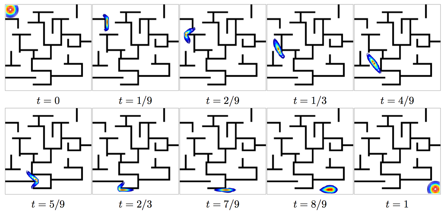
Refer to caption
Figure 7.3: Solution αtsubscript𝛼𝑡\alpha_{t} of dynamic OT computed with a proximal splitting scheme.

7.4 Dynamical Unbalanced OT

In order to be able to match input measures with different mass α0(𝒳)α1(𝒳)subscript𝛼0𝒳subscript𝛼1𝒳\alpha_{0}(\mathcal{X})\neq\alpha_{1}(\mathcal{X}) (the so-called “unbalanced” settings, the terminology introduced by Benamou (2003)), and also to cope with local mass variation, several normalizations or relaxations have been proposed, in particular by relaxing the fixed marginal constraint; see §10.2. A general methodology consists in introducing a source term st(x)subscript𝑠𝑡𝑥s_{t}(x) in the continuity equation (7.4). We thus consider

𝒞¯(α0,α1)=def.{(αt,Jt,st):αtt+div(Jt)=st,αt=0=α0,αt=1=α1}.superscriptdef.¯𝒞subscript𝛼0subscript𝛼1conditional-setsubscript𝛼𝑡subscript𝐽𝑡subscript𝑠𝑡formulae-sequencesubscript𝛼𝑡𝑡divsubscript𝐽𝑡subscript𝑠𝑡formulae-sequencesubscript𝛼𝑡0subscript𝛼0subscript𝛼𝑡1subscript𝛼1\bar{\mathcal{C}}(\alpha_{0},\alpha_{1})\stackrel{{\scriptstyle\mbox{\tiny def.}}}{{=}}\left\{(\alpha_{t},J_{t},s_{t})\;:\;\frac{\partial\alpha_{t}}{\partial t}+\operatorname{div}(J_{t})=s_{t},\alpha_{t=0}=\alpha_{0},\alpha_{t=1}=\alpha_{1}\right\}.

The crucial question is how to measure the cost associated to this source term and introduce it in the original dynamic formulation (7.3). Several proposals appear in the literature, for instance, using an L2superscript𝐿2L^{2} cost Piccoli and Rossi (2014). In order to avoid having to “teleport” mass (mass which travels at infinite speed and suddenly grows in a region where there was no mass before), the associated cost should be infinite. It turns out that this can be achieved in a simple convex way, by also allowing stsubscript𝑠𝑡s_{t} to be an arbitrary measure (e.g. using a 1-homogeneous cost) by penalizing stsubscript𝑠𝑡s_{t} in the same way as the momentum Jtsubscript𝐽𝑡J_{t},

WFR2(α0,α1)=min(αt,Jt,st)t𝒞¯(α0,α1)Θ(α,J,s),superscriptWFR2subscript𝛼0subscript𝛼1subscriptsubscript𝛼𝑡subscript𝐽𝑡subscript𝑠𝑡𝑡¯𝒞subscript𝛼0subscript𝛼1Θ𝛼𝐽𝑠\operatorname{WFR}^{2}(\alpha_{0},\alpha_{1})=\underset{(\alpha_{t},J_{t},s_{t})_{t}\in\bar{\mathcal{C}}(\alpha_{0},\alpha_{1})}{\min}\;\Theta(\alpha,J,s), (7.15)
whereΘ(α,J,s)=def.01d(θ(αt(x),Jt(x))+τθ(αt(x),st(x)))dxdt,superscriptdef.whereΘ𝛼𝐽𝑠superscriptsubscript01subscriptsuperscript𝑑𝜃subscript𝛼𝑡𝑥subscript𝐽𝑡𝑥𝜏𝜃subscript𝛼𝑡𝑥subscript𝑠𝑡𝑥differential-d𝑥differential-d𝑡\quad\text{where}\quad\Theta(\alpha,J,s)\stackrel{{\scriptstyle\mbox{\tiny def.}}}{{=}}\int_{0}^{1}\int_{\mathbb{R}^{d}}\left(\theta(\alpha_{t}(x),J_{t}(x))+\tau\theta(\alpha_{t}(x),s_{t}(x))\right)\mathrm{d}x\mathrm{d}t,

where θ𝜃\theta is the convex 1-homogeneous function introduced in (7.5), and τ𝜏\tau is a weight controlling the trade-off between mass transportation and mass creation/destruction. This formulation was proposed independently by several authors (Liero et al., 2016; Chizat et al., 2018c; Kondratyev et al., 2016). This “dynamic” formulation has a “static” counterpart; see Remark 5. The convex optimization problem (7.15) can be solved using methods similar to those detailed in §7.3. Figure 7.4 displays a comparison of several unbalanced OT dynamic interpolations. This dynamic formulation resembles “metamorphosis” models for shape registration (Trouvé and Younes, 2005), and a more precise connection is detailed in (Maas et al., 2015, 2016).

As τ0𝜏0\tau\rightarrow 0, and if α0(𝒳)=α1(𝒳)subscript𝛼0𝒳subscript𝛼1𝒳\alpha_{0}(\mathcal{X})=\alpha_{1}(\mathcal{X}), then one retrieves the classical OT problem, WFR(α0,α1)𝒲(α0,α1)WFRsubscript𝛼0subscript𝛼1𝒲subscript𝛼0subscript𝛼1\operatorname{WFR}(\alpha_{0},\alpha_{1})\rightarrow\operatorname{\mathcal{W}}(\alpha_{0},\alpha_{1}). In contrast, as τ+𝜏\tau\rightarrow+\infty, this distance approaches the Hellinger metric over densities
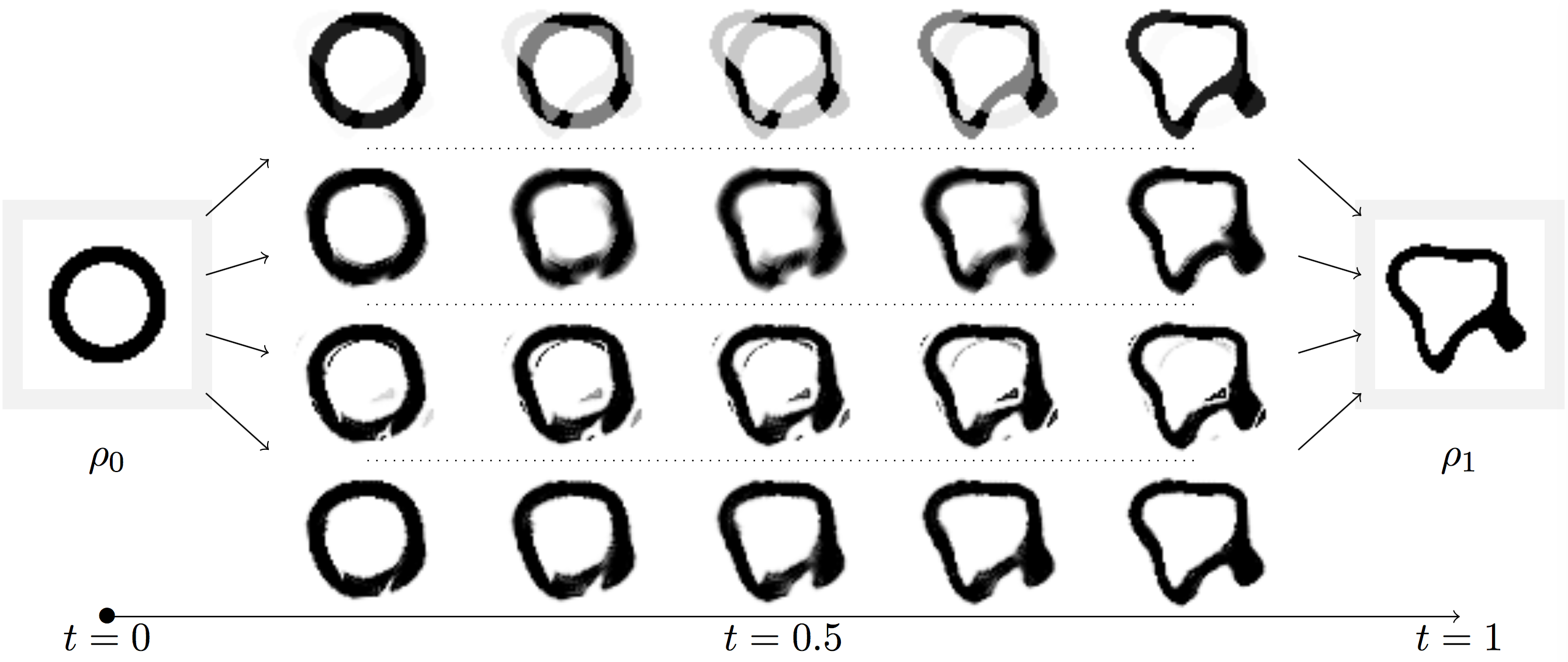
1τWFR(α0,α1)2τ+\displaystyle\frac{1}{\tau}\operatorname{WFR}(\alpha_{0},\alpha_{1})^{2}\;\overset{\tau\rightarrow+\infty}{\longrightarrow} 𝒳|ρα0(x)ρα1(x)|2dxsubscript𝒳superscriptsubscript𝜌subscript𝛼0𝑥subscript𝜌subscript𝛼1𝑥2differential-d𝑥\displaystyle\int_{\mathcal{X}}|\sqrt{\rho_{\alpha_{0}}(x)}-\sqrt{\rho_{\alpha_{1}}(x)}|^{2}\mathrm{d}x
=\displaystyle= 𝒳|1dα1dα0(x)|2dα0(x).subscript𝒳superscript1dsubscript𝛼1dsubscript𝛼0𝑥2differential-dsubscript𝛼0𝑥\displaystyle\int_{\mathcal{X}}|1-\sqrt{\frac{\mathrm{d}\alpha_{1}}{\mathrm{d}\alpha_{0}}(x)}|^{2}\mathrm{d}\alpha_{0}(x).
Refer to caption
Figure 7.4: Comparison of Hellinger (first row), Wasserstein (row 2), partial optimal transport (row 3), and Wasserstein–Fisher–Rao (row 4) dynamic interpolations.

7.5 More General Mobility Functionals

It is possible to generalize the dynamic formulation (7.3) by considering other “mobility functions” θ𝜃\theta in place of the one defined in (7.5). A possible choice for this mobility functional is proposed in Dolbeault et al. (2009),

(a,b)+×d,θ(a,b)=aspbp,formulae-sequencefor-all𝑎𝑏subscriptsuperscript𝑑𝜃𝑎𝑏superscript𝑎𝑠𝑝superscriptnorm𝑏𝑝\forall\,(a,b)\in\mathbb{R}_{+}\times\mathbb{R}^{d},\quad\theta(a,b)=a^{s-p}\left\|b\right\|^{p}, (7.16)

where the parameter should satisfy p1𝑝1p\geq 1 and s[1,p]𝑠1𝑝s\in[1,p] in order for θ𝜃\theta to be convex. Note that this definition should be handled with care in the case 1<sp1𝑠𝑝1<s\leq p because θ𝜃\theta does not have a linear growth at infinity, so that solutions to (7.3) must be constrained to have a density with respect to the Lebesgue measure.

The case s=1𝑠1s=1 corresponds to the classical OT problem and the optimal value of (7.3) defines 𝒲p(α,β)subscript𝒲𝑝𝛼𝛽\operatorname{\mathcal{W}}_{p}(\alpha,\beta). In this case, θ𝜃\theta is 1-homogeneous, so that solutions to (7.3) can be arbitrary measures. The case (s=1,p=2)formulae-sequence𝑠1𝑝2(s=1,p=2) is the initial setup considered in (7.3) to define 𝒲2subscript𝒲2\operatorname{\mathcal{W}}_{2}.

The limiting case s=p𝑠𝑝s=p is also interesting, because it corresponds to a dual Sobolev norm W1,psuperscript𝑊1𝑝W^{-1,p} and the value of (7.3) is then equal to

αβW1,p(d)p=min𝑓{dfd(αβ):df(x)qdx1}superscriptsubscriptnorm𝛼𝛽superscript𝑊1𝑝superscript𝑑𝑝𝑓conditional-setsubscriptsuperscript𝑑𝑓d𝛼𝛽subscriptsuperscript𝑑superscriptnorm𝑓𝑥𝑞differential-d𝑥1\left\|\alpha-\beta\right\|_{W^{-1,p}(\mathbb{R}^{d})}^{p}=\underset{f}{\min}\;\left\{\int_{\mathbb{R}^{d}}f\mathrm{d}(\alpha-\beta)\;:\;\int_{\mathbb{R}^{d}}\left\|\nabla f(x)\right\|^{q}\mathrm{d}x\leq 1\right\}

for 1/q+1/p=11𝑞1𝑝11/q+1/p=1. In the limit (p=s,q)(1,)𝑝𝑠𝑞1(p=s,q)\rightarrow(1,\infty), one recovers the 𝒲1subscript𝒲1\operatorname{\mathcal{W}}_{1} norm. The case s=p=2𝑠𝑝2s=p=2 corresponds to the Sobolev H1(d)superscript𝐻1superscript𝑑H^{-1}(\mathbb{R}^{d}) Hilbert norm defined in (8.15).

7.6 Dynamic Formulation over the Paths Space

There is a natural dynamical formulation of both classical and entropic regularized (see §4) formulations of OT, which is based on studying abstract optimization problems on the space 𝒳¯¯𝒳\bar{\mathcal{X}} of all possible paths γ:[0,1]𝒳:𝛾01𝒳\gamma:[0,1]\rightarrow\mathcal{X} (i.e. curves) on the space 𝒳𝒳\mathcal{X}. For simplicity, we assume 𝒳=d𝒳superscript𝑑\mathcal{X}=\mathbb{R}^{d}, but this extends to more general spaces such as geodesic spaces and graphs. Informally, the dynamic of “particles” between two input measures α0,α1subscript𝛼0subscript𝛼1\alpha_{0},\alpha_{1} at times t=0,1𝑡01t=0,1 is described by a probability distribution π¯+1(𝒳¯)¯𝜋superscriptsubscript1¯𝒳\bar{\pi}\in\mathcal{M}_{+}^{1}(\bar{\mathcal{X}}). Such a distribution should satisfy that the distributions of starting and end points must match (α0,α1)subscript𝛼0subscript𝛼1(\alpha_{0},\alpha_{1}), which is formally written using push-forward as

𝒰¯(α0,α1)=def.{π¯+1(𝒳¯):P¯0π¯=α0,P¯1π¯=α1},superscriptdef.¯𝒰subscript𝛼0subscript𝛼1conditional-set¯𝜋superscriptsubscript1¯𝒳formulae-sequencesubscript¯𝑃0¯𝜋subscript𝛼0subscript¯𝑃1¯𝜋subscript𝛼1\bar{\mathcal{U}}(\alpha_{0},\alpha_{1})\stackrel{{\scriptstyle\mbox{\tiny def.}}}{{=}}\left\{\bar{\pi}\in\mathcal{M}_{+}^{1}(\bar{\mathcal{X}})\;:\;\bar{P}_{0\sharp}\bar{\pi}=\alpha_{0},\bar{P}_{1\sharp}\bar{\pi}=\alpha_{1}\right\},

where, for any path γ𝒳¯𝛾¯𝒳\gamma\in\bar{\mathcal{X}}, P0(γ)=γ(0),P1(γ)=γ(1)formulae-sequencesubscript𝑃0𝛾𝛾0subscript𝑃1𝛾𝛾1P_{0}(\gamma)=\gamma(0),P_{1}(\gamma)=\gamma(1).

OT over the space of paths.

The dynamical version of classical OT (2.15), formulated over the space of paths, then reads

𝒲2(α0,α1)2=minπ¯𝒰¯(α0,α1)𝒳¯(γ)2dπ¯(γ),\operatorname{\mathcal{W}}_{2}(\alpha_{0},\alpha_{1})^{2}=\underset{\bar{\pi}\in\bar{\mathcal{U}}(\alpha_{0},\alpha_{1})}{\min}\;\int_{\bar{\mathcal{X}}}\mathcal{L}(\gamma)^{2}\mathrm{d}\bar{\pi}(\gamma), (7.17)

where (γ)=01|γ(s)|2ds𝛾superscriptsubscript01superscriptsuperscript𝛾𝑠2differential-d𝑠\mathcal{L}(\gamma)=\int_{0}^{1}|\gamma^{\prime}(s)|^{2}\mathrm{d}s is the kinetic energy of a path s[0,1]γ(s)𝒳𝑠01maps-to𝛾𝑠𝒳s\in[0,1]\mapsto\gamma(s)\in\mathcal{X}. The connection between optimal couplings πsuperscript𝜋\pi^{\star} and π¯superscript¯𝜋\bar{\pi}^{\star} solving respectively (7.17) and (2.15) is that π¯superscript¯𝜋\bar{\pi}^{\star} only gives mass to geodesics joining pairs of points in proportion prescribed by πsuperscript𝜋\pi^{\star}. In the particular case of discrete measures, this means that

π=i,jPi,jδ(xi,yj)andπ¯=i,jPi,jδγxi,yj,formulae-sequencesuperscript𝜋subscript𝑖𝑗subscriptP𝑖𝑗subscript𝛿subscript𝑥𝑖subscript𝑦𝑗andsuperscript¯𝜋subscript𝑖𝑗subscriptP𝑖𝑗subscript𝛿subscript𝛾subscript𝑥𝑖subscript𝑦𝑗\pi^{\star}=\sum_{i,j}\mathrm{\textbf{P}}_{i,j}\delta_{(x_{i},y_{j})}\quad\text{and}\quad\bar{\pi}^{\star}=\sum_{i,j}\mathrm{\textbf{P}}_{i,j}\delta_{\gamma_{x_{i},y_{j}}},

where γxi,yjsubscript𝛾subscript𝑥𝑖subscript𝑦𝑗\gamma_{x_{i},y_{j}} is the geodesic between xisubscript𝑥𝑖x_{i} and yjsubscript𝑦𝑗y_{j}. Furthermore, the measures defined by the distribution of the curve points γ(t)𝛾𝑡\gamma(t) at time t𝑡t, where γ𝛾\gamma is drawn following π¯superscript¯𝜋\bar{\pi}^{\star}, i.e.

t[0,1]αt=def.Ptπ¯wherePt(γ)=γ(t)𝒳,formulae-sequence𝑡01maps-tosubscript𝛼𝑡superscriptdef.subscript𝑃𝑡superscript¯𝜋wheresubscript𝑃𝑡𝛾𝛾𝑡𝒳t\in[0,1]\mapsto\alpha_{t}\stackrel{{\scriptstyle\mbox{\tiny def.}}}{{=}}P_{t\sharp}\bar{\pi}^{\star}\quad\text{where}\quad P_{t}(\gamma)=\gamma(t)\in\mathcal{X}, (7.18)

is a solution to the dynamical formulation (7.3), i.e. it is the displacement interpolation. In the discrete case, one recovers (7.9).

Entropic OT over the space of paths.

We now turn to the re-interpretation of entropic OT, defined in Chapter 4, using the space of paths. Similarly to (4.11), this is defined using a Kullback–Leibler projection, but this time of a reference measure over the space of paths 𝒦¯¯𝒦\bar{\mathcal{K}} which is the distribution of a reversible Brownian motion (Wiener process), which has a uniform distribution at the initial and final times

minπ¯𝒰¯(α0,α1)KL(π¯|𝒦¯).¯𝜋¯𝒰subscript𝛼0subscript𝛼1KLconditional¯𝜋¯𝒦\underset{\bar{\pi}\in\bar{\mathcal{U}}(\alpha_{0},\alpha_{1})}{\min}\;\operatorname{KL}(\bar{\pi}|\bar{\mathcal{K}}). (7.19)

We refer to the review paper by Léonard (2014) for an overview of this problem and an historical account of the work of Schrödinger (1931). One can show that the (unique) solution π¯εsuperscriptsubscript¯𝜋𝜀\bar{\pi}_{\varepsilon}^{\star} to (7.19) converges to a solution of (7.17) as ε0𝜀0\varepsilon\rightarrow 0. Furthermore, this solution is linked to the solution of the static entropic OT problem (4.9) using Brownian bridge γ¯x,yε𝒳¯superscriptsubscript¯𝛾𝑥𝑦𝜀¯𝒳\bar{\gamma}_{x,y}^{\varepsilon}\in\bar{\mathcal{X}} (which are similar to fuzzy geodesic and converge to δγx,ysubscript𝛿subscript𝛾𝑥𝑦\delta_{\gamma_{x,y}} as ε0𝜀0\varepsilon\rightarrow 0). In the discrete setting, this means that

πε=i,jPε,i,jδ(xi,yj)andπ¯ε=i,jPε,i,jγ¯xi,yjε,formulae-sequencesuperscriptsubscript𝜋𝜀subscript𝑖𝑗superscriptsubscriptP𝜀𝑖𝑗subscript𝛿subscript𝑥𝑖subscript𝑦𝑗andsuperscriptsubscript¯𝜋𝜀subscript𝑖𝑗superscriptsubscriptP𝜀𝑖𝑗superscriptsubscript¯𝛾subscript𝑥𝑖subscript𝑦𝑗𝜀\pi_{\varepsilon}^{\star}=\sum_{i,j}\mathrm{\textbf{P}}_{\varepsilon,i,j}^{\star}\delta_{(x_{i},y_{j})}\quad\text{and}\quad\bar{\pi}_{\varepsilon}^{\star}=\sum_{i,j}\mathrm{\textbf{P}}_{\varepsilon,i,j}^{\star}\bar{\gamma}_{x_{i},y_{j}}^{\varepsilon}, (7.20)

where Pε,i,jsuperscriptsubscriptP𝜀𝑖𝑗\mathrm{\textbf{P}}_{\varepsilon,i,j}^{\star} can be computed using Sinkhorn’s algorithm. Similarly to (7.18), one then can define an entropic interpolation as

αε,t=def.Ptπ¯ε.superscriptdef.subscript𝛼𝜀𝑡subscriptP𝑡superscriptsubscript¯𝜋𝜀\alpha_{\varepsilon,t}\stackrel{{\scriptstyle\mbox{\tiny def.}}}{{=}}\mathrm{\textbf{P}}_{t\sharp}\bar{\pi}_{\varepsilon}^{\star}.

Since the law Ptγ¯x,yεsubscriptP𝑡superscriptsubscript¯𝛾𝑥𝑦𝜀\mathrm{\textbf{P}}_{t\sharp}\bar{\gamma}_{x,y}^{\varepsilon} of the position at time t𝑡t along a Brownian bridge is a Gaussian 𝒢t(1t)ε2(γx,y(t))\mathcal{G}_{t(1-t)\varepsilon^{2}}(\cdot-\gamma_{x,y}(t)) of variance t(1t)ε2𝑡1𝑡superscript𝜀2t(1-t)\varepsilon^{2} centered at γx,y(t)subscript𝛾𝑥𝑦𝑡\gamma_{x,y}(t), one can deduce that αε,tsubscript𝛼𝜀𝑡\alpha_{\varepsilon,t} is a Gaussian blurring of a set of traveling Diracs

αε,t=i,jPε,i,j𝒢t(1t)ε2(γxi,yj(t)).\alpha_{\varepsilon,t}=\sum_{i,j}\mathrm{\textbf{P}}_{\varepsilon,i,j}^{\star}\mathcal{G}_{t(1-t)\varepsilon^{2}}(\cdot-\gamma_{x_{i},y_{j}}(t)).

The resulting mixture of Brownian bridges is displayed on Figure 7.5.
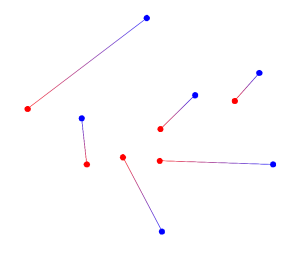
Refer to caption Refer to caption Refer to caption Refer to caption
ε=0𝜀0\varepsilon=0 ε=.05𝜀.05\varepsilon=.05 ε=0.2𝜀0.2\varepsilon=0.2 ε=1𝜀1\varepsilon=1
Figure 7.5: Samples from Brownian bridge paths associated to the Schrödinger entropic interpolation (7.20) over path space. Blue corresponds to t=0𝑡0t=0 and red to t=1𝑡1t=1.

Another way to describe this entropic interpolation (αt)tsubscriptsubscript𝛼𝑡𝑡(\alpha_{t})_{t} is using a regularization of the Benamou–Brenier dynamic formulation (7.2), namely

min(αt,vt)t sat. (7.1)01d(vt(x)2+ε4log(αt)(x)2)dαt(x)dt;subscriptsubscript𝛼𝑡subscript𝑣𝑡𝑡 sat. (7.1)superscriptsubscript01subscriptsuperscript𝑑superscriptnormsubscript𝑣𝑡𝑥2𝜀4superscriptnormsubscript𝛼𝑡𝑥2differential-dsubscript𝛼𝑡𝑥differential-d𝑡\underset{(\alpha_{t},v_{t})_{t}\text{ sat. \eqref{eq-cons-bb-ncvx}}}{\min}\;\int_{0}^{1}\int_{\mathbb{R}^{d}}\left(\left\|v_{t}(x)\right\|^{2}+\frac{\varepsilon}{4}\left\|\nabla\log(\alpha_{t})(x)\right\|^{2}\right)\mathrm{d}\alpha_{t}(x)\mathrm{d}t; (7.21)

see (Gentil et al., 2015; Chen et al., 2016a).

Chapter 8 Statistical Divergences

We study in this chapter the statistical properties of the Wasserstein distance. More specifically, we compare it to other major distances and divergences routinely used in data sciences. We quantify how one can approximate the distance between two probability distributions when having only access to samples from said distributions. To introduce these subjects, §8.1 and §8.2 review respectively divergences and integral probability metrics between probability distributions. A divergence D𝐷D typically satisfies D(α,β)0𝐷𝛼𝛽0D(\alpha,\beta)\geq 0 and D(α,β)=0𝐷𝛼𝛽0D(\alpha,\beta)=0 if and only if α=β𝛼𝛽\alpha=\beta, but it does not need to be symmetric or satisfy the triangular inequality. An integral probability metric for measures is a dual norm defined using a prescribed family of test functions. These quantities are sound alternatives to Wasserstein distances and are routinely used as loss functions to tackle inference problems, as will be covered in §9. We show first in §8.3 that the optimal transport distance is not Hilbertian, i.e. one cannot approximate it efficiently using a Hilbertian metric on a suitable feature representation of probability measures. We show in §8.4 how to approximate D(α,β)𝐷𝛼𝛽D(\alpha,\beta) from discrete samples (xi)isubscriptsubscript𝑥𝑖𝑖(x_{i})_{i} and (yj)jsubscriptsubscript𝑦𝑗𝑗(y_{j})_{j} drawn from α𝛼\alpha and β𝛽\beta. A good statistical understanding of that problem is crucial when using the Wasserstein distance in machine learning. Note that this section will be chiefly concerned with the statistical approximation of optimal transport between distributions supported on continuous sets. The very same problem when the ground space is finite has received some attention in the literature following the work of Sommerfeld and Munk (2018), extended to entropic regularized quantities by Bigot et al. (2017a).

8.1 φ𝜑\varphi-Divergences

Before detailing in the following section “weak” norms, whose construction shares similarities with 𝒲1subscript𝒲1\operatorname{\mathcal{W}}_{1}, let us detail a generic construction of so-called divergences between measures, which can then be used as loss functions when estimating probability distributions. Such divergences compare two input measures by comparing their mass pointwise, without introducing any notion of mass transportation. Divergences are functionals which, by looking at the pointwise ratio between two measures, give a sense of how close they are. They have nice analytical and computational properties and build upon entropy functions.

Definition 8.1 (Entropy function).

A function φ:{}:𝜑\varphi:\mathbb{R}\to\mathbb{R}\cup\{\infty\} is an entropy function if it is lower semicontinuous, convex, domφ[0,[\operatorname{dom}\varphi\subset[0,\infty[, and satisfies the following feasibility condition: domφ]0,[\operatorname{dom}\varphi\;\cap\;]0,\infty[\;\neq\emptyset. The speed of growth of φ𝜑\varphi at \infty is described by

φ=limx+φ(x)/x{}.subscriptsuperscript𝜑subscript𝑥𝜑𝑥𝑥\varphi^{\prime}_{\infty}=\lim_{x\rightarrow+\infty}\varphi(x)/x\in\mathbb{R}\cup\{\infty\}\,.

If φ=subscriptsuperscript𝜑\varphi^{\prime}_{\infty}=\infty, then φ𝜑\varphi grows faster than any linear function and φ𝜑\varphi is said superlinear. Any entropy function φ𝜑\varphi induces a φ𝜑\varphi-divergence (also known as Ciszár divergence (Ciszár, 1967; Ali and Silvey, 1966) or f𝑓f-divergence) as follows.

Definition 8.2 (φ𝜑\varphi-Divergences).

Let φ𝜑\varphi be an entropy function. For α,β(𝒳)𝛼𝛽𝒳\alpha,\beta\in\mathcal{M}(\mathcal{X}), let dαdββ+αd𝛼d𝛽𝛽superscript𝛼perpendicular-to\frac{\mathrm{d}\alpha}{\mathrm{d}\beta}\beta+\alpha^{\perp} be the Lebesgue decomposition111The Lebesgue decomposition theorem asserts that, given β𝛽\beta, α𝛼\alpha admits a unique decomposition as the sum of two measures αs+αsuperscript𝛼𝑠superscript𝛼perpendicular-to\alpha^{s}+\alpha^{\perp} such that αssuperscript𝛼𝑠\alpha^{s} is absolutely continuous with respect to β𝛽\beta and αsuperscript𝛼perpendicular-to\alpha^{\perp} and β𝛽\beta are singular. of α𝛼\alpha with respect to β𝛽\beta. The divergence 𝒟φsubscript𝒟𝜑\mathcal{D}_{\varphi} is defined by

𝒟φ(α|β)=def.𝒳φ(dαdβ)dβ+φα(𝒳)superscriptdef.subscript𝒟𝜑conditional𝛼𝛽subscript𝒳𝜑d𝛼d𝛽differential-d𝛽subscriptsuperscript𝜑superscript𝛼perpendicular-to𝒳\mathcal{D}_{\varphi}(\alpha|\beta)\stackrel{{\scriptstyle\mbox{\tiny def.}}}{{=}}\int_{\mathcal{X}}\varphi\left(\frac{\mathrm{d}\alpha}{\mathrm{d}\beta}\right)\mathrm{d}\beta+\varphi^{\prime}_{\infty}\alpha^{\perp}(\mathcal{X}) (8.1)

if α,β𝛼𝛽\alpha,\beta are nonnegative and \infty otherwise.

The additional term φα(𝒳)subscriptsuperscript𝜑superscript𝛼perpendicular-to𝒳\varphi^{\prime}_{\infty}\alpha^{\perp}(\mathcal{X}) in (8.1) is important to ensure that 𝒟φsubscript𝒟𝜑\mathcal{D}_{\varphi} defines a continuous functional (for the weak topology of measures) even if φ𝜑\varphi has a linear growth at infinity, as this is, for instance, the case for the absolute value (8.8) defining the TV norm. If φ𝜑\varphi as a superlinear growth, e.g. the usual entropy (8.4), then φ=+subscriptsuperscript𝜑\varphi^{\prime}_{\infty}=+\infty so that 𝒟φ(α|β)=+subscript𝒟𝜑conditional𝛼𝛽\mathcal{D}_{\varphi}(\alpha|\beta)=+\infty if α𝛼\alpha does not have a density with respect to β𝛽\beta.

In the discrete setting, assuming

α=iaiδxiandβ=ibiδxiformulae-sequence𝛼subscript𝑖subscripta𝑖subscript𝛿subscript𝑥𝑖and𝛽subscript𝑖subscriptb𝑖subscript𝛿subscript𝑥𝑖\alpha=\sum_{i}\mathrm{\textbf{a}}_{i}\delta_{x_{i}}\quad\text{and}\quad\beta=\sum_{i}\mathrm{\textbf{b}}_{i}\delta_{x_{i}} (8.2)

are supported on the same set of n𝑛n points (xi)i=1n𝒳superscriptsubscriptsubscript𝑥𝑖𝑖1𝑛𝒳(x_{i})_{i=1}^{n}\subset\mathcal{X}, (8.1) defines a divergence on ΣnsubscriptΣ𝑛\Sigma_{n}

Dφ(a|b)=iSupp(b)φ(aibi)bi+φiSupp(b)ai,subscriptD𝜑conditionalabsubscript𝑖Suppb𝜑subscripta𝑖subscriptb𝑖subscriptb𝑖subscriptsuperscript𝜑subscript𝑖Suppbsubscripta𝑖\mathrm{\textbf{D}}_{\varphi}(\mathrm{\textbf{a}}|\mathrm{\textbf{b}})=\sum_{i\in\operatorname{Supp}(\mathrm{\textbf{b}})}\varphi\left(\frac{\mathrm{\textbf{a}}_{i}}{\mathrm{\textbf{b}}_{i}}\right)\mathrm{\textbf{b}}_{i}+\varphi^{\prime}_{\infty}\sum_{i\notin\operatorname{Supp}(\mathrm{\textbf{b}})}\mathrm{\textbf{a}}_{i}, (8.3)

where Supp(b)=def.{in:bi0}\operatorname{Supp}(\mathrm{\textbf{b}})\stackrel{{\scriptstyle\mbox{\tiny def.}}}{{=}}\left\{i\in\llbracket n\rrbracket\;:\;b_{i}\neq 0\right\}.

The proof of the following proposition can be found in (Liero et al., 2018, Thm 2.7).

Proposition 8.1.1.

If φ𝜑\varphi is an entropy function, then 𝒟φsubscript𝒟𝜑\mathcal{D}_{\varphi} is jointly 111-homogeneous, convex and weakly* lower semicontinuous in (α,β)𝛼𝛽(\alpha,\beta).

Refer to caption
Figure 8.1: Example of entropy functionals.
Remark 1 (Dual expression).

A φ𝜑\varphi-divergence can be expressed using the Legendre transform

φ(s)=def.suptstφ(t)superscriptdef.superscript𝜑𝑠𝑡supremum𝑠𝑡𝜑𝑡\varphi^{*}(s)\stackrel{{\scriptstyle\mbox{\tiny def.}}}{{=}}\underset{t\in\mathbb{R}}{\sup}\;st-\varphi(t)

of φ𝜑\varphi (see also (4.54)) as

𝒟φ(α|β)=supf:𝒳𝒳f(x)dα(x)𝒳φ(f(x))dβ(x);subscript𝒟𝜑conditional𝛼𝛽:𝑓𝒳supremumsubscript𝒳𝑓𝑥differential-d𝛼𝑥subscript𝒳superscript𝜑𝑓𝑥differential-d𝛽𝑥\mathcal{D}_{\varphi}(\alpha|\beta)=\underset{f:\mathcal{X}\rightarrow\mathbb{R}}{\sup}\;\int_{\mathcal{X}}f(x)\mathrm{d}\alpha(x)-\int_{\mathcal{X}}\varphi^{*}(f(x))\mathrm{d}\beta(x);

see Liero et al. (2018) for more details.

We now review a few popular instances of this framework. Figure 8.1 displays the associated entropy functionals, while Figure 8.2 reviews the relationship between them.
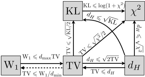
Refer to caption
Figure 8.2: Diagram of relationship between divergences (inspired by Gibbs and Su (2002)). For 𝒳𝒳\mathcal{X} a metric space with ground distance d𝑑d, dmax=sup(x,x)d(x,x)subscript𝑑subscriptsupremum𝑥superscript𝑥𝑑𝑥superscript𝑥d_{\max}=\sup_{(x,x^{\prime})}d(x,x^{\prime}) is the diameter of 𝒳𝒳\mathcal{X}. When 𝒳𝒳\mathcal{X} is discrete, dmin=def.minxxd(x,x)superscriptdef.subscript𝑑subscript𝑥superscript𝑥𝑑𝑥superscript𝑥d_{\min}\stackrel{{\scriptstyle\mbox{\tiny def.}}}{{=}}\min_{x\neq x^{\prime}}d(x,x^{\prime}).
Example 8.1.2 (Kullback–Leibler divergence).

The Kullback–Leibler divergence KL=def.𝒟φKLsuperscriptdef.KLsubscript𝒟subscript𝜑KL\operatorname{KL}\stackrel{{\scriptstyle\mbox{\tiny def.}}}{{=}}\mathcal{D}_{\varphi_{\operatorname{KL}}}, also known as the relative entropy, was already introduced in (4.10) and (4.6). It is the divergence associated to the Shannon–Boltzman entropy function φKLsubscript𝜑KL\varphi_{\operatorname{KL}}, given by

φKL(s)={slog(s)s+1for s>0,1for s=0,+otherwise.subscript𝜑KL𝑠cases𝑠𝑠𝑠1for 𝑠01for 𝑠0otherwise.\varphi_{\operatorname{KL}}(s)=\begin{cases}s\log(s)-s+1&\textnormal{for }s>0,\\ 1&\textnormal{for }s=0,\\ +\infty&\textnormal{otherwise.}\end{cases} (8.4)
Remark 8.1.3 (Bregman divergence).

The discrete KL divergence, KL=def.DφKLsuperscriptdef.KLsubscriptDsubscript𝜑KL\mathrm{\textbf{KL}}\stackrel{{\scriptstyle\mbox{\tiny def.}}}{{=}}\mathrm{\textbf{D}}_{\varphi_{\operatorname{KL}}}, has the unique property of being both a φ𝜑\varphi-divergence and a Bregman divergence. For discrete vectors in nsuperscript𝑛\mathbb{R}^{n}, a Bregman divergence (Bregman, 1967) associated to a smooth strictly convex function ψ:n:𝜓superscript𝑛\psi:\mathbb{R}^{n}\rightarrow\mathbb{R} is defined as

Bψ(a|b)=def.ψ(a)ψ(b)ψ(b),ab,superscriptdef.subscriptB𝜓conditionalab𝜓a𝜓b𝜓bab\mathrm{\textbf{B}}_{\psi}(\mathrm{\textbf{a}}|\mathrm{\textbf{b}})\stackrel{{\scriptstyle\mbox{\tiny def.}}}{{=}}\psi(\mathrm{\textbf{a}})-\psi(\mathrm{\textbf{b}})-\langle\nabla\psi(\mathrm{\textbf{b}}),\,\mathrm{\textbf{a}}-\mathrm{\textbf{b}}\rangle, (8.5)

where ,\langle\cdot,\,\cdot\rangle is the canonical inner product on nsuperscript𝑛\mathbb{R}^{n}. Note that Bψ(a|b)subscriptB𝜓conditionalab\mathrm{\textbf{B}}_{\psi}(\mathrm{\textbf{a}}|\mathrm{\textbf{b}}) is a convex function of a and a linear function of ψ𝜓\psi. Similarly to φ𝜑\varphi-divergence, a Bregman divergence satisfies Bψ(a|b)0subscriptB𝜓conditionalab0\mathrm{\textbf{B}}_{\psi}(\mathrm{\textbf{a}}|\mathrm{\textbf{b}})\geq 0 and Bψ(a|b)=0subscriptB𝜓conditionalab0\mathrm{\textbf{B}}_{\psi}(\mathrm{\textbf{a}}|\mathrm{\textbf{b}})=0 if and only if a=bab\mathrm{\textbf{a}}=\mathrm{\textbf{b}}. The KL divergence is the Bregman divergence for minus the entropy ψ=H𝜓H\psi=-\mathrm{\textbf{H}} defined in (4.1)), i.e. KL=BHKLsubscriptBH\mathrm{\textbf{KL}}=\mathrm{\textbf{B}}_{-\mathrm{\textbf{H}}}. A Bregman divergence is locally a squared Euclidean distance since

Bψ(a+ε|a+η)=2ψ(a)(εη),εη+o(εη2)subscriptB𝜓aconditional𝜀a𝜂superscript2𝜓a𝜀𝜂𝜀𝜂𝑜superscriptnorm𝜀𝜂2\mathrm{\textbf{B}}_{\psi}(\mathrm{\textbf{a}}+\varepsilon|\mathrm{\textbf{a}}+\eta)=\langle\partial^{2}\psi(\mathrm{\textbf{a}})(\varepsilon-\eta),\,\varepsilon-\eta\rangle+o(\left\|\varepsilon-\eta\right\|^{2})

and the set of separating points {a:Bψ(a|b)=Bψ(a|b)}conditional-setasubscriptB𝜓conditionalabsubscriptB𝜓conditionalasuperscriptb\left\{\mathrm{\textbf{a}}\;:\;\mathrm{\textbf{B}}_{\psi}(\mathrm{\textbf{a}}|\mathrm{\textbf{b}})=\mathrm{\textbf{B}}_{\psi}(\mathrm{\textbf{a}}|\mathrm{\textbf{b}}^{\prime})\right\} is a hyperplane between b and bsuperscriptb\mathrm{\textbf{b}}^{\prime}. These properties make Bregman divergence suitable to replace Euclidean distances in first order optimization methods. The best know example is mirror gradient descent (Beck and Teboulle, 2003), which is an explicit descent step of the form (9.32). Bregman divergences are also important in convex optimization and can be used, for instance, to derive Sinkhorn iterations and study its convergence in finite dimension; see Remark 4.8.

Remark 8.1.4 (Hyperbolic geometry of KL).

It is interesting to contrast the geometry of the Kullback–Leibler divergence to that defined by quadratic optimal transport when comparing Gaussians. As detailed, for instance, by Costa et al. (2015), the Kullback–Leibler divergence has a closed form for Gaussian densities. In the univariate case, d=1𝑑1d=1, if α=𝒩(mα,σα2)𝛼𝒩subscript𝑚𝛼superscriptsubscript𝜎𝛼2\alpha=\mathcal{N}(m_{\alpha},\sigma_{\alpha}^{2}) and β=𝒩(mβ,σβ2)𝛽𝒩subscript𝑚𝛽superscriptsubscript𝜎𝛽2\beta=\mathcal{N}(m_{\beta},\sigma_{\beta}^{2}), one has

KL(α|β)=12(σα2σβ2+log(σβ2σα2)+|mαmβ|σβ21).KLconditional𝛼𝛽12superscriptsubscript𝜎𝛼2superscriptsubscript𝜎𝛽2superscriptsubscript𝜎𝛽2superscriptsubscript𝜎𝛼2subscript𝑚𝛼subscript𝑚𝛽superscriptsubscript𝜎𝛽21\operatorname{KL}(\alpha|\beta)=\frac{1}{2}\left(\frac{\sigma_{\alpha}^{2}}{\sigma_{\beta}^{2}}+\log\left(\frac{\sigma_{\beta}^{2}}{\sigma_{\alpha}^{2}}\right)+\frac{|m_{\alpha}-m_{\beta}|}{\sigma_{\beta}^{2}}-1\right). (8.6)

This expression shows that the divergence between α𝛼\alpha and β𝛽\beta diverges to infinity as σβsubscript𝜎𝛽\sigma_{\beta} diminishes to 00 and β𝛽\beta becomes a Dirac mass. In that sense, one can say that singular Gaussians are infinitely far from all other Gaussians in the KL geometry. That geometry is thus useful when one wants to avoid dealing with singular covariances. To simplify the analysis, one can look at the infinitesimal geometry of KL, which is obtained by performing a Taylor expansion at order 2,

KL(𝒩(m+δm,(σ+δσ)2)|𝒩(m,σ2))=1σ2(12δm2+δσ2)+o(δm2,δσ2).KLconditional𝒩𝑚subscript𝛿𝑚superscript𝜎subscript𝛿𝜎2𝒩𝑚superscript𝜎21superscript𝜎212superscriptsubscript𝛿𝑚2superscriptsubscript𝛿𝜎2𝑜superscriptsubscript𝛿𝑚2superscriptsubscript𝛿𝜎2\operatorname{KL}(\mathcal{N}(m+\delta_{m},(\sigma+\delta_{\sigma})^{2})|\mathcal{N}(m,\sigma^{2}))=\frac{1}{\sigma^{2}}\left(\frac{1}{2}\delta_{m}^{2}+\delta_{\sigma}^{2}\right)+o(\delta_{m}^{2},\delta_{\sigma}^{2}).

This local Riemannian metric, the so-called Fisher metric, expressed over (m/2,σ)×+,𝑚2𝜎subscript(m/\sqrt{2},\sigma)\in\mathbb{R}\times\mathbb{R}_{+,*}, matches exactly that of the hyperbolic Poincaré half plane. Geodesics over this space are half circles centered along the σ=0𝜎0\sigma=0 line and have an exponential speed, i.e. they only reach the limit σ=0𝜎0\sigma=0 after an infinite time. Note in particular that if σα=σβsubscript𝜎𝛼subscript𝜎𝛽\sigma_{\alpha}=\sigma_{\beta} but mαmαsubscript𝑚𝛼subscript𝑚𝛼m_{\alpha}\neq m_{\alpha}, then the geodesic between (α,β)𝛼𝛽(\alpha,\beta) over this hyperbolic half plane does not have a constant standard deviation.

The KL hyperbolic geometry over the space of Gaussian parameters (m,σ)𝑚𝜎(m,\sigma) should be contrasted with the Euclidean geometry associated to OT as described in Remark 2.31, since in the univariate case

𝒲22(α,β)=|mαmβ|2+|σασβ|2.superscriptsubscript𝒲22𝛼𝛽superscriptsubscript𝑚𝛼subscript𝑚𝛽2superscriptsubscript𝜎𝛼subscript𝜎𝛽2\operatorname{\mathcal{W}}_{2}^{2}(\alpha,\beta)=|m_{\alpha}-m_{\beta}|^{2}+|\sigma_{\alpha}-\sigma_{\beta}|^{2}. (8.7)

Figure 8.3 shows a visual comparison of these two geometries and their respective geodesics. This interesting comparison was suggested to us by Jean Feydy.
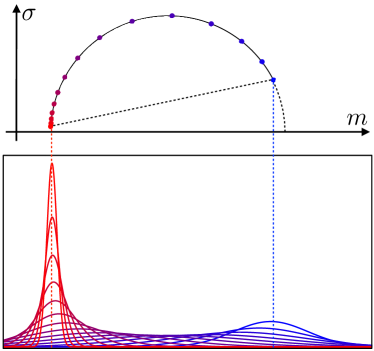
Refer to caption Refer to caption
KL OT
Figure 8.3: Comparisons of interpolation between Gaussians using KL (hyperbolic) and OT (Euclidean) geometries.
Example 8.1.5 (Total variation).

The total variation distance TV=def.𝒟φTVsuperscriptdef.TVsubscript𝒟subscript𝜑TV\operatorname{TV}\stackrel{{\scriptstyle\mbox{\tiny def.}}}{{=}}\mathcal{D}_{\varphi_{\operatorname{TV}}} is the divergence associated to

φTV(s)={|s1|for s0,+otherwise.subscript𝜑TV𝑠cases𝑠1for 𝑠0otherwise.\varphi_{\operatorname{TV}}(s)=\begin{cases}|s-1|&\textnormal{for }s\geq 0,\\ +\infty&\textnormal{otherwise.}\end{cases} (8.8)

It actually defines a norm on the full space of measure (𝒳)𝒳\mathcal{M}(\mathcal{X}) where

TV(α|β)=αβTV,whereαTV=|α|(𝒳)=𝒳d|α|(x).formulae-sequenceTVconditional𝛼𝛽subscriptnorm𝛼𝛽TVwheresubscriptnorm𝛼TV𝛼𝒳subscript𝒳d𝛼𝑥\operatorname{TV}(\alpha|\beta)=\left\|\alpha-\beta\right\|_{\operatorname{TV}},\quad\text{where}\quad\left\|\alpha\right\|_{\operatorname{TV}}=|\alpha|(\mathcal{X})=\int_{\mathcal{X}}\mathrm{d}|\alpha|(x). (8.9)

If α𝛼\alpha has a density ραsubscript𝜌𝛼\rho_{\alpha} on 𝒳=d𝒳superscript𝑑\mathcal{X}=\mathbb{R}^{d}, then the TV norm is the L1superscript𝐿1L^{1} norm on functions, αTV=𝒳|ρα(x)|dx=ραL1subscriptnorm𝛼TVsubscript𝒳subscript𝜌𝛼𝑥differential-d𝑥subscriptnormsubscript𝜌𝛼superscript𝐿1\left\|\alpha\right\|_{\operatorname{TV}}=\int_{\mathcal{X}}|\rho_{\alpha}(x)|\mathrm{d}x=\left\|\rho_{\alpha}\right\|_{L^{1}}. If α𝛼\alpha is discrete as in (8.2), then the TV norm is the 1superscript1\ell^{1} norm of vectors in nsuperscript𝑛\mathbb{R}^{n}, αTV=i|ai|=a1subscriptnorm𝛼TVsubscript𝑖subscripta𝑖subscriptnormasuperscript1\left\|\alpha\right\|_{\operatorname{TV}}=\sum_{i}|\mathrm{\textbf{a}}_{i}|=\left\|\mathrm{\textbf{a}}\right\|_{\ell^{1}}.

Remark 2 (Strong vs. weak topology).

The total variation norm (8.9) defines the so-called “strong” topology on the space of measure. On a compact domain 𝒳𝒳\mathcal{X} of radius R𝑅R, one has

𝒲1(α,β)RαβTVsubscript𝒲1𝛼𝛽𝑅subscriptnorm𝛼𝛽TV\operatorname{\mathcal{W}}_{1}(\alpha,\beta)\leq R\left\|\alpha-\beta\right\|_{\operatorname{TV}}

so that this strong notion of convergence implies the weak convergence metrized by Wasserstein distances. The converse is, however, not true, since δxsubscript𝛿𝑥\delta_{x} does not converge strongly to δysubscript𝛿𝑦\delta_{y} if xy𝑥𝑦x\rightarrow y (note that δxδyTV=2subscriptnormsubscript𝛿𝑥subscript𝛿𝑦TV2\left\|\delta_{x}-\delta_{y}\right\|_{\operatorname{TV}}=2 if xy𝑥𝑦x\neq y). A chief advantage is that +1(𝒳)superscriptsubscript1𝒳\mathcal{M}_{+}^{1}(\mathcal{X}) (once again on a compact ground space 𝒳𝒳\mathcal{X}) is compact for the weak topology, so that from any sequence of probability measures (αk)ksubscriptsubscript𝛼𝑘𝑘(\alpha_{k})_{k}, one can always extract a converging subsequence, which makes it a suitable space for several optimization problems, such as those considered in Chapter 9.

Example 8.1.6 (Hellinger).

The Hellinger distance 𝔥=def.𝒟φH1/2superscriptdef.𝔥superscriptsubscript𝒟subscript𝜑𝐻12\mathfrak{h}\stackrel{{\scriptstyle\mbox{\tiny def.}}}{{=}}\mathcal{D}_{\varphi_{H}}^{1/2} is the square root of the divergence associated to

φH(s)={|s1|2for s0,+otherwise.subscript𝜑𝐻𝑠casessuperscript𝑠12for 𝑠0otherwise.\varphi_{H}(s)=\begin{cases}|\sqrt{s}-1|^{2}&\textnormal{for }s\geq 0,\\ +\infty&\textnormal{otherwise.}\end{cases}

As its name suggests, 𝔥𝔥\mathfrak{h} is a distance on +(𝒳)subscript𝒳\mathcal{M}_{+}(\mathcal{X}), which metrizes the strong topology as TV\left\|\cdot\right\|_{\operatorname{TV}}. If (α,β)𝛼𝛽(\alpha,\beta) have densities (ρα,ρβ)subscript𝜌𝛼subscript𝜌𝛽(\rho_{\alpha},\rho_{\beta}) on 𝒳=d𝒳superscript𝑑\mathcal{X}=\mathbb{R}^{d}, then 𝔥(α,β)=ραρβL2𝔥𝛼𝛽subscriptnormsubscript𝜌𝛼subscript𝜌𝛽superscript𝐿2\mathfrak{h}(\alpha,\beta)=\|\sqrt{\rho_{\alpha}}-\sqrt{\rho_{\beta}}\|_{L^{2}}. If (α,β)𝛼𝛽(\alpha,\beta) are discrete as in (8.2), then 𝔥(α,β)=ab𝔥𝛼𝛽normab\mathfrak{h}(\alpha,\beta)=\|\sqrt{\mathrm{\textbf{a}}}-\sqrt{\mathrm{\textbf{b}}}\|. Considering φLp(s)=|s1/p1|psubscript𝜑superscript𝐿𝑝𝑠superscriptsuperscript𝑠1𝑝1𝑝\varphi_{L^{p}}(s)=|s^{1/p}-1|^{p} generalizes the Hellinger (p=2𝑝2p=2) and total variation (p=1𝑝1p=1) distances and 𝒟φLp1/psuperscriptsubscript𝒟subscript𝜑superscript𝐿𝑝1𝑝\mathcal{D}_{\varphi_{L^{p}}}^{1/p} is a distance which metrizes the strong convergence for 0<p<+0𝑝0<p<+\infty.

Example 8.1.7 (Jensen–Shannon distance).

The KL divergence is not symmetric and, while being a Bregman divergence (which are locally quadratic norms), it is not the square of a distance. On the other hand, the Jensen–Shannon distance JS(α,β)JS𝛼𝛽\text{JS}(\alpha,\beta), defined as

JS(α,β)2=def.12(KL(α|ξ)+KL(β|ξ))whereξ=α+β2,formulae-sequencesuperscriptdef.JSsuperscript𝛼𝛽212KLconditional𝛼𝜉KLconditional𝛽𝜉where𝜉𝛼𝛽2\text{JS}(\alpha,\beta)^{2}\stackrel{{\scriptstyle\mbox{\tiny def.}}}{{=}}\frac{1}{2}\left(\operatorname{KL}(\alpha|\xi)+\operatorname{KL}(\beta|\xi)\right)\quad\text{where}\quad\xi=\frac{\alpha+\beta}{2},

is a distance (Endres and Schindelin, 2003; Österreicher and Vajda, 2003). JS2superscriptJS2\text{JS}^{2} can be shown to be a φ𝜑\varphi-divergence for φ(s)=tlog(t)(t+1)log(t+1)𝜑𝑠𝑡𝑡𝑡1𝑡1\varphi(s)=t\log(t)-(t+1)\log(t+1). In sharp contrast with KLKL\operatorname{KL}, JS(α,β)JS𝛼𝛽\text{JS}(\alpha,\beta) is always bounded; more precisely, it satisfies 0JS(α,β)2ln(2)0JSsuperscript𝛼𝛽220\leq\text{JS}(\alpha,\beta)^{2}\leq\ln(2). Similarly to the TV norm and the Hellinger distance, it metrizes the strong convergence.

Example 8.1.8 (χ2superscript𝜒2\chi^{2}).

The χ2superscript𝜒2\chi^{2}-divergence χ2=def.𝒟φχ2superscriptdef.superscript𝜒2subscript𝒟subscript𝜑superscript𝜒2\chi^{2}\stackrel{{\scriptstyle\mbox{\tiny def.}}}{{=}}\mathcal{D}_{\varphi_{\chi^{2}}} is the divergence associated to

φχ2(s)={|s1|2for s0,+otherwise.subscript𝜑superscript𝜒2𝑠casessuperscript𝑠12for 𝑠0otherwise.\varphi_{\chi^{2}}(s)=\begin{cases}|s-1|^{2}&\textnormal{for }s\geq 0,\\ +\infty&\textnormal{otherwise.}\end{cases}

If (α,β)𝛼𝛽(\alpha,\beta) are discrete as in (8.2) and have the same support, then

χ2(α|β)=i(aibi)2bi.superscript𝜒2conditional𝛼𝛽subscript𝑖superscriptsubscripta𝑖subscriptb𝑖2subscriptb𝑖\chi^{2}(\alpha|\beta)=\sum_{i}\frac{(\mathrm{\textbf{a}}_{i}-\mathrm{\textbf{b}}_{i})^{2}}{\mathrm{\textbf{b}}_{i}}.

8.2 Integral Probability Metrics

Formulation (6.3) is a special case of a dual norm. A dual norm is a convenient way to design “weak” norms that can deal with arbitrary measures. For a symmetric convex set B𝐵B of measurable functions, one defines

αB=def.max𝑓{𝒳f(x)dα(x):fB}.superscriptdef.subscriptnorm𝛼𝐵𝑓conditional-setsubscript𝒳𝑓𝑥differential-d𝛼𝑥𝑓𝐵\left\|\alpha\right\|_{B}\stackrel{{\scriptstyle\mbox{\tiny def.}}}{{=}}\underset{f}{\max}\;\left\{\int_{\mathcal{X}}f(x)\mathrm{d}\alpha(x)\;:\;f\in B\right\}. (8.10)

These dual norms are often called “integral probability metrics’; see (Sriperumbudur et al., 2012).

Example 8.2.1 (Total variation).

The total variation norm (Example 8.1.5) is a dual norm associated to the whole space of continuous functions

B={f𝒞(𝒳):f1}.𝐵conditional-set𝑓𝒞𝒳subscriptnorm𝑓1B=\left\{f\in\mathcal{C}(\mathcal{X})\;:\;\left\|f\right\|_{\infty}\leq 1\right\}.

The total variation distance is the only nontrivial divergence that is also a dual norm; see (Sriperumbudur et al., 2009).

Remark 3 (Metrizing the weak convergence).

By using smaller “balls” B𝐵B, which typically only contain continuous (and sometimes regular) functions, one defines weaker dual norms. In order for B\left\|\cdot\right\|_{B} to metrize the weak convergence (see Definition 2.2), it is sufficient for the space spanned by B𝐵B to be dense in the set of continuous functions for the sup-norm \left\|\cdot\right\|_{\infty} (i.e. for the topology of uniform convergence); see (Ambrosio et al., 2006, para. 5.1).

Figure 8.4 displays a comparison of several such dual norms, which we now detail.
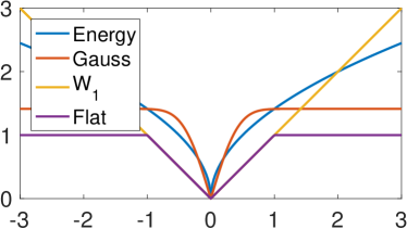
Refer to caption Refer to caption
(α,β)=(δ0,δt)𝛼𝛽subscript𝛿0subscript𝛿𝑡(\alpha,\beta)=(\delta_{0},\delta_{t}) (α,β)=(δ0,12(δt/2+δt/2))𝛼𝛽subscript𝛿012subscript𝛿𝑡2subscript𝛿𝑡2(\alpha,\beta)=(\delta_{0},\frac{1}{2}(\delta_{-t/2}+\delta_{t/2}))
Figure 8.4: Comparison of dual norms.

8.2.1 𝒲1subscript𝒲1\operatorname{\mathcal{W}}_{1} and Flat Norm

If the set B𝐵B is bounded, then B\left\|\cdot\right\|_{B} is a norm on the whole space (𝒳)𝒳\mathcal{M}(\mathcal{X}) of measures. This is not the case of 𝒲1subscript𝒲1\operatorname{\mathcal{W}}_{1}, which is only defined for α𝛼\alpha such that 𝒳dα=0subscript𝒳differential-d𝛼0\int_{\mathcal{X}}\mathrm{d}\alpha=0 (otherwise αB=+subscriptnorm𝛼𝐵\left\|\alpha\right\|_{B}=+\infty). This can be alleviated by imposing a bound on the value of the potential f𝑓f, in order to define for instance the flat norm.

Example 8.2.2 (𝒲1subscript𝒲1\operatorname{\mathcal{W}}_{1} norm).

𝒲1subscript𝒲1\operatorname{\mathcal{W}}_{1} as defined in (6.3), is a special case of dual norm (8.10), using

B={f:Lip(f)1}𝐵conditional-set𝑓Lip𝑓1B=\left\{f\;:\;\operatorname{Lip}(f)\leq 1\right\}

the set of 1-Lipschitz functions.

Example 8.2.3 (Flat norm and Dudley metric).

The flat norm is defined using

B={f:f1andf1}.𝐵conditional-set𝑓formulae-sequencesubscriptnorm𝑓1andsubscriptnorm𝑓1B=\left\{f\;:\;\left\|\nabla f\right\|_{\infty}\leq 1\quad\text{and}\quad\left\|f\right\|_{\infty}\leq 1\right\}. (8.11)

It metrizes the weak convergence on the whole space (𝒳)𝒳\mathcal{M}(\mathcal{X}). Formula (6.2) is extended to compute the flat norm by adding the constraint |fk|1subscriptf𝑘1\left\lvert\mathrm{\textbf{f}}_{k}\right\rvert\leq 1. The flat norm is sometimes called the “Kantorovich–Rubinstein” norm (Hanin, 1992) and has been used as a fidelity term for inverse problems in imaging (Lellmann et al., 2014). The flat norm is similar to the Dudley metric, which uses

B={f:f+f1}.𝐵conditional-set𝑓subscriptnorm𝑓subscriptnorm𝑓1B=\left\{f\;:\;\left\|\nabla f\right\|_{\infty}+\left\|f\right\|_{\infty}\leq 1\right\}.

8.2.2 Dual RKHS Norms and Maximum Mean Discrepancies

It is also possible to define “Euclidean” norms (built using quadratic functionals) on measures using the machinery of kernel methods and more specifically reproducing kernel Hilbert spaces (RKHS; see (Schölkopf and Smola, 2002) for a survey of their applications in data sciences), of which we recall first some basic definitions.

Definition 4.

A symmetric function k𝑘k (resp., φ𝜑\varphi) defined on a set 𝒳×𝒳𝒳𝒳\mathcal{X}\times\mathcal{X} is said to be positive (resp., negative) definite if for any n0𝑛0n\geq 0, family x1,,xn𝒵subscript𝑥1subscript𝑥𝑛𝒵x_{1},\dots,x_{n}\in\mathcal{Z}, and vector rn𝑟superscript𝑛r\in\mathbb{R}^{n} the following inequality holds:

i,j=1nrirjk(xi,xj)0,(resp.i,j=1nrirjφ(xi,xj)0).superscriptsubscript𝑖𝑗1𝑛subscript𝑟𝑖subscript𝑟𝑗𝑘subscript𝑥𝑖subscript𝑥𝑗0resp.superscriptsubscript𝑖𝑗1𝑛subscript𝑟𝑖subscript𝑟𝑗𝜑subscript𝑥𝑖subscript𝑥𝑗0\sum_{i,j=1}^{n}r_{i}r_{j}k(x_{i},x_{j})\geq 0,\quad\left(\text{resp.}\quad\sum_{i,j=1}^{n}r_{i}r_{j}\varphi(x_{i},x_{j})\leq 0\right). (8.12)

The kernel is said to be conditionally positive if positivity only holds in (8.12) for zero mean vectors r𝑟r (i.e. such that r,𝟙n=0𝑟subscriptdouble-struck-𝟙𝑛0\langle r,\,\mathbb{1}_{n}\rangle=0).

If k𝑘k is conditionally positive, one defines the following norm:

αk2=def.𝒳×𝒳k(x,y)dα(x)dα(y).superscriptdef.subscriptsuperscriptnorm𝛼2𝑘subscript𝒳𝒳𝑘𝑥𝑦differential-d𝛼𝑥differential-d𝛼𝑦\left\|\alpha\right\|^{2}_{k}\stackrel{{\scriptstyle\mbox{\tiny def.}}}{{=}}\int_{\mathcal{X}\times\mathcal{X}}k(x,y)\mathrm{d}\alpha(x)\mathrm{d}\alpha(y). (8.13)

These norms are often referred to as “maximum mean discrepancy” (MMD) (see (Gretton et al., 2007)) and have also been called “kernel norms” in shape analysis (Glaunes et al., 2004). This expression (8.13) can be rephrased, introducing two independent random vectors (X,X)𝑋superscript𝑋(X,X^{\prime}) on 𝒳𝒳\mathcal{X} distributed with law α𝛼\alpha, as

αk2=𝔼X,X(k(X,X)).subscriptsuperscriptnorm𝛼2𝑘subscript𝔼𝑋superscript𝑋𝑘𝑋superscript𝑋\left\|\alpha\right\|^{2}_{k}=\mathbb{E}_{X,X^{\prime}}(k(X,X^{\prime})).

One can show that k2\left\|\cdot\right\|^{2}_{k} is the dual norm in the sense of (8.10) associated to the unit ball B𝐵B of the RKHS associated to k𝑘k. We refer to (Berlinet and Thomas-Agnan, 2003; Hofmann et al., 2008; Schölkopf and Smola, 2002) for more details on RKHS functional spaces.

Remark 5 (Universal kernels).

According to Remark 3, the MMD norm k\left\|\cdot\right\|_{k} metrizes the weak convergence if the span of the dual ball B𝐵B is dense in the space of continuous functions 𝒞(𝒳)𝒞𝒳\mathcal{C}(\mathcal{X}). This means that finite sums of the form i=1naik(xi,)superscriptsubscript𝑖1𝑛subscript𝑎𝑖𝑘subscript𝑥𝑖\sum_{i=1}^{n}a_{i}k(x_{i},\cdot) (for arbitrary choice of n𝑛n and points (xi)isubscriptsubscript𝑥𝑖𝑖(x_{i})_{i}) are dense in 𝒞(𝒳)𝒞𝒳\mathcal{C}(\mathcal{X}) for the uniform norm \left\|\cdot\right\|_{\infty}. For translation-invariant kernels over 𝒳=d𝒳superscript𝑑\mathcal{X}=\mathbb{R}^{d}, k(x,y)=k0(xy)𝑘𝑥𝑦subscript𝑘0𝑥𝑦k(x,y)=k_{0}(x-y), this is equivalent to having a nonvanishing Fourier transform, k^0(ω)>0subscript^𝑘0𝜔0\hat{k}_{0}(\omega)>0.

In the special case where α𝛼\alpha is a discrete measure of the form (2.3), one thus has the simple expression

αk2=i=1ni=1naiaiki,i=ka,awhereki,i=def.k(xi,xi).formulae-sequencesuperscriptsubscriptnorm𝛼𝑘2superscriptsubscript𝑖1𝑛superscriptsubscriptsuperscript𝑖1𝑛subscripta𝑖subscriptasuperscript𝑖subscriptk𝑖superscript𝑖kaasuperscriptdef.wheresubscriptk𝑖superscript𝑖𝑘subscript𝑥𝑖subscript𝑥superscript𝑖\left\|\alpha\right\|_{k}^{2}=\sum_{i=1}^{n}\sum_{i^{\prime}=1}^{n}\mathrm{\textbf{a}}_{i}\mathrm{\textbf{a}}_{i^{\prime}}\mathrm{\textbf{k}}_{i,i^{\prime}}=\langle\mathrm{\textbf{k}}\mathrm{\textbf{a}},\,\mathrm{\textbf{a}}\rangle\quad\text{where}\quad\mathrm{\textbf{k}}_{i,i^{\prime}}\stackrel{{\scriptstyle\mbox{\tiny def.}}}{{=}}k(x_{i},x_{i^{\prime}}).

In particular, when α=i=1naiδxi𝛼superscriptsubscript𝑖1𝑛subscripta𝑖subscript𝛿subscript𝑥𝑖\alpha=\sum_{i=1}^{n}\mathrm{\textbf{a}}_{i}\delta_{x_{i}} and β=i=1nbiδxi𝛽superscriptsubscript𝑖1𝑛subscriptb𝑖subscript𝛿subscript𝑥𝑖\beta=\sum_{i=1}^{n}\mathrm{\textbf{b}}_{i}\delta_{x_{i}} are supported on the same set of points, αβk2=k(ab),absuperscriptsubscriptnorm𝛼𝛽𝑘2kabab\left\|\alpha-\beta\right\|_{k}^{2}=\langle\mathrm{\textbf{k}}(\mathrm{\textbf{a}}-\mathrm{\textbf{b}}),\,\mathrm{\textbf{a}}-\mathrm{\textbf{b}}\rangle, so that k\left\|\cdot\right\|_{k} is a Euclidean norm (proper if k is positive definite, degenerate otherwise if k is semidefinite) on the simplex ΣnsubscriptΣ𝑛\Sigma_{n}. To compute the discrepancy between two discrete measures of the form (2.3), one can use

αβk2=i,iaiaik(xi,xi)+j,jbjbjk(yj,yj)2i,jaibjk(xi,yj).superscriptsubscriptnorm𝛼𝛽𝑘2subscript𝑖superscript𝑖subscripta𝑖subscriptasuperscript𝑖𝑘subscript𝑥𝑖subscript𝑥superscript𝑖subscript𝑗superscript𝑗subscriptb𝑗subscriptbsuperscript𝑗𝑘subscript𝑦𝑗subscript𝑦superscript𝑗2subscript𝑖𝑗subscripta𝑖subscriptb𝑗𝑘subscript𝑥𝑖subscript𝑦𝑗\left\|\alpha-\beta\right\|_{k}^{2}=\sum_{i,i^{\prime}}\mathrm{\textbf{a}}_{i}\mathrm{\textbf{a}}_{i^{\prime}}k(x_{i},x_{i^{\prime}})+\sum_{j,j^{\prime}}\mathrm{\textbf{b}}_{j}\mathrm{\textbf{b}}_{j^{\prime}}k(y_{j},y_{j^{\prime}})-2\sum_{i,j}\mathrm{\textbf{a}}_{i}\mathrm{\textbf{b}}_{j}k(x_{i},y_{j}). (8.14)
Example 8.2.4 (Gaussian RKHS).

One of the most popular kernels is the Gaussian one k(x,y)=exy22σ2𝑘𝑥𝑦superscript𝑒superscriptnorm𝑥𝑦22superscript𝜎2k(x,y)=e^{-\frac{\left\|x-y\right\|^{2}}{2\sigma^{2}}}, which is a positive universal kernel on 𝒳=d𝒳superscript𝑑\mathcal{X}=\mathbb{R}^{d}. An attractive feature of the Gaussian kernel is that it is separable as a product of 1-D kernels, which facilitates computations when working on regular grids (see also Remark 4.17). However, an important issue that arises when using the Gaussian kernel is that one needs to select the bandwidth parameter σ𝜎\sigma. This bandwidth should match the “typical scale” between observations in the measures to be compared. If the measures have multiscale features (some regions may be very dense, others very sparsely populated), a Gaussian kernel is thus not well adapted, and one should consider a “scale-free” kernel as we detail next. An issue with such scale-free kernels is that they are global (have slow polynomial decay), which makes them typically computationally more expensive, since no compact support approximation is possible. Figure 8.5 shows a comparison between several kernels.
Refer to caption Refer to caption Refer to caption Refer to caption
Refer to caption Refer to caption Refer to caption Refer to caption Refer to caption
(α,β)𝛼𝛽({\color[rgb]{1,0,0}\alpha},{\color[rgb]{0,0,1}\beta}) ED(2,)\text{ED}(\mathbb{R}^{2},\left\|\cdot\right\|) (G,.005)𝐺.005(G,.005) (G,.02)𝐺.02(G,.02) (G,.05)𝐺.05(G,.05)
Figure 8.5: Top row: display of ψ𝜓\psi such that αβk=ψ(αβ)L2(2)subscriptnorm𝛼𝛽𝑘subscriptnorm𝜓𝛼𝛽superscript𝐿2superscript2\left\|\alpha-\beta\right\|_{k}=\left\|\psi\star(\alpha-\beta)\right\|_{L^{2}(\mathbb{R}^{2})}, formally defined over Fourier as ψ^(ω)=k^0(ω)^𝜓𝜔subscript^𝑘0𝜔\hat{\psi}(\omega)=\sqrt{\hat{k}_{0}(\omega)}, where k(x,x)=k0(xx)𝑘𝑥superscript𝑥subscript𝑘0𝑥superscript𝑥k(x,x^{\prime})=k_{0}(x-x^{\prime}). Bottom row: display of ψ(αβ)𝜓𝛼𝛽\psi\star(\alpha-\beta). (G,σ𝜎\sigma) stands for Gaussian kernel of variance σ2superscript𝜎2\sigma^{2}. The kernel for ED(2,)\text{ED}(\mathbb{R}^{2},\left\|\cdot\right\|) is ψ(x)=1/x𝜓𝑥1norm𝑥\psi(x)=1/\sqrt{\left\|x\right\|}.
Example 8.2.5 (H1(d)superscript𝐻1superscript𝑑H^{-1}(\mathbb{R}^{d})).

Another important dual norm is H1(d)superscript𝐻1superscript𝑑H^{-1}(\mathbb{R}^{d}), the dual (over distributions) of the Sobolev space H1(d)superscript𝐻1superscript𝑑H^{1}(\mathbb{R}^{d}) of functions having derivatives in L2(d)superscript𝐿2superscript𝑑L^{2}(\mathbb{R}^{d}). It is defined using the primal RKHS norm fL2(d)2superscriptsubscriptnorm𝑓superscript𝐿2superscript𝑑2\left\|\nabla f\right\|_{L^{2}(\mathbb{R}^{d})}^{2}. It is not defined for singular measures (e.g. Diracs) unless d=1𝑑1d=1 because functions in the Sobolev space H1(d)superscript𝐻1superscript𝑑H^{1}(\mathbb{R}^{d}) are in general not continuous. This H1superscript𝐻1H^{-1} norm (defined on the space of zero mean measures with densities) can also be formulated in divergence form,

αβH1(d)2=min𝑠{ds(x)22dx:div(s)=αβ},superscriptsubscriptnorm𝛼𝛽superscript𝐻1superscript𝑑2𝑠conditional-setsubscriptsuperscript𝑑:evaluated-at𝑠𝑥22d𝑥div𝑠𝛼𝛽\left\|\alpha-\beta\right\|_{H^{-1}(\mathbb{R}^{d})}^{2}=\underset{s}{\min}\;\left\{\int_{\mathbb{R}^{d}}\left\|s(x)\right\|_{2}^{2}\mathrm{d}x\;:\;\operatorname{div}(s)=\alpha-\beta\right\}, (8.15)

which should be contrasted with (6.4), where an L1superscript𝐿1L^{1} norm of the vector field s𝑠s was used in place of the L2superscript𝐿2L^{2} norm used here. The “weighted” version of this Sobolev dual norm,

ρH1(α)2=mindiv(s)=ρds(x)22dα(x),superscriptsubscriptnorm𝜌superscript𝐻1𝛼2div𝑠𝜌subscriptsuperscript𝑑superscriptsubscriptnorm𝑠𝑥22differential-d𝛼𝑥\left\|\rho\right\|_{H^{-1}(\alpha)}^{2}=\underset{\operatorname{div}(s)=\rho}{\min}\;\int_{\mathbb{R}^{d}}\left\|s(x)\right\|_{2}^{2}\mathrm{d}\alpha(x),

can be interpreted as the natural “linearization” of the Wasserstein 𝒲2subscript𝒲2\operatorname{\mathcal{W}}_{2} norm, in the sense that the Benamou–Brenier dynamic formulation can be interpreted infinitesimally as

𝒲2(α,α+ερ)=ερH1(α)+o(ε).subscript𝒲2𝛼𝛼𝜀𝜌𝜀subscriptnorm𝜌superscript𝐻1𝛼𝑜𝜀\operatorname{\mathcal{W}}_{2}(\alpha,\alpha+\varepsilon\rho)=\varepsilon\left\|\rho\right\|_{H^{-1}(\alpha)}+o(\varepsilon). (8.16)

The functionals 𝒲2(α,β)subscript𝒲2𝛼𝛽\operatorname{\mathcal{W}}_{2}(\alpha,\beta) and αβH1(α)subscriptnorm𝛼𝛽superscript𝐻1𝛼\left\|\alpha-\beta\right\|_{H^{-1}(\alpha)} can be shown to be equivalent (Peyre, 2011). The issue is that αβH1(α)subscriptnorm𝛼𝛽superscript𝐻1𝛼\left\|\alpha-\beta\right\|_{H^{-1}(\alpha)} is not a norm (because of the weighting by α𝛼\alpha), and one cannot in general replace it by αβH1(d)subscriptnorm𝛼𝛽superscript𝐻1superscript𝑑\left\|\alpha-\beta\right\|_{H^{-1}(\mathbb{R}^{d})} unless (α,β)𝛼𝛽(\alpha,\beta) have densities. In this case, if α𝛼\alpha and β𝛽\beta have densities on the same support bounded from below by a>0𝑎0a>0 and from above by b<+𝑏b<+\infty, then

b1/2αβH1(d)W2(α,β)a1/2αβH1(d);superscript𝑏12subscriptnorm𝛼𝛽superscript𝐻1superscript𝑑subscript𝑊2𝛼𝛽superscript𝑎12subscriptnorm𝛼𝛽superscript𝐻1superscript𝑑b^{-1/2}\left\|\alpha-\beta\right\|_{H^{-1}(\mathbb{R}^{d})}\leq W_{2}(\alpha,\beta)\leq a^{-1/2}\left\|\alpha-\beta\right\|_{H^{-1}(\mathbb{R}^{d})}; (8.17)

see (Santambrogio, 2015, Theo. 5.34), and see (Peyre, 2011) for sharp constants.

Example 8.2.6 (Negative Sobolev spaces).

One can generalize this construction by considering the Sobolev space Hr(d)superscript𝐻𝑟superscript𝑑H^{-r}(\mathbb{R}^{d}) of arbitrary negative index, which is the dual of the functional Sobolev space Hr(d)superscript𝐻𝑟superscript𝑑H^{r}(\mathbb{R}^{d}) of functions having r𝑟r derivatives (in the sense of distributions) in L2(d)superscript𝐿2superscript𝑑L^{2}(\mathbb{R}^{d}). In order to metrize the weak convergence, one needs functions in Hr(d)superscript𝐻𝑟superscript𝑑H^{r}(\mathbb{R}^{d}) to be continuous, which is the case when r>d/2𝑟𝑑2r>d/2. As the dimension d𝑑d increases, one thus needs to consider higher regularity. For arbitrary α𝛼\alpha (not necessarily integers), these spaces are defined using the Fourier transform, and for a measure α𝛼\alpha with Fourier transform α^(ω)^𝛼𝜔\hat{\alpha}(\omega) (written here as a density with respect to the Lebesgue measure dωd𝜔\mathrm{d}\omega)

αHr(d)2=def.dω2r|α^(ω)|2dω.superscriptdef.superscriptsubscriptnorm𝛼superscript𝐻𝑟superscript𝑑2subscriptsuperscript𝑑superscriptnorm𝜔2𝑟superscript^𝛼𝜔2differential-d𝜔\left\|\alpha\right\|_{H^{-r}(\mathbb{R}^{d})}^{2}\stackrel{{\scriptstyle\mbox{\tiny def.}}}{{=}}\int_{\mathbb{R}^{d}}\left\|\omega\right\|^{-2r}|\hat{\alpha}(\omega)|^{2}\mathrm{d}\omega.

This corresponds to a dual RKHS norm with a convolutive kernel k(x,y)=k0(xy)𝑘𝑥𝑦subscript𝑘0𝑥𝑦k(x,y)=k_{0}(x-y) with k^0(ω)=±ω2rsubscript^𝑘0𝜔plus-or-minussuperscriptnorm𝜔2𝑟\hat{k}_{0}(\omega)=\pm\left\|\omega\right\|^{-2r}. Taking the inverse Fourier transform, one sees that (up to constant) one has

xd,k0(x)={1xd2rifr<d/2,x2rdifr>d/2.formulae-sequencefor-all𝑥superscript𝑑subscript𝑘0𝑥cases1superscriptnorm𝑥𝑑2𝑟if𝑟𝑑2superscriptnorm𝑥2𝑟𝑑if𝑟𝑑2\forall\,x\in\mathbb{R}^{d},\quad k_{0}(x)=\left\{\begin{array}[]{l}\frac{1}{\left\|x\right\|^{d-2r}}\quad\text{if}\quad r<d/2,\\ -\left\|x\right\|^{2r-d}\quad\text{if}\quad r>d/2.\end{array}\right. (8.18)
Example 8.2.7 (Energy distance).

The energy distance (or Cramer distance when d=1𝑑1d=1(Székely and Rizzo, 2004) associated to a distance d𝑑d is defined as

αβED(𝒳,dp)=def.αβkEDwherekED(x,y)=d(x,y)pformulae-sequencesuperscriptdef.subscriptnorm𝛼𝛽ED𝒳superscript𝑑𝑝subscriptnorm𝛼𝛽subscript𝑘EDwheresubscript𝑘ED𝑥𝑦𝑑superscript𝑥𝑦𝑝\left\|\alpha-\beta\right\|_{\text{ED}(\mathcal{X},d^{p})}\stackrel{{\scriptstyle\mbox{\tiny def.}}}{{=}}\left\|\alpha-\beta\right\|_{k_{\text{ED}}}\quad\text{where}\quad k_{\text{ED}}(x,y)=-d(x,y)^{p} (8.19)

for 0<p<20𝑝20<p<2. It is a valid MMD norm over measures if d𝑑d is negative definite (see Definition 4), a typical example being the Euclidean distance d(x,y)=xy𝑑𝑥𝑦norm𝑥𝑦d(x,y)=\left\|x-y\right\|. For 𝒳=d𝒳superscript𝑑\mathcal{X}=\mathbb{R}^{d}, d(x,y)=d(x,y)=\left\|\cdot\right\|, using (8.18), one sees that the energy distance is a Sobolev norm

ED(d,p)=Hd+p2(d).\left\|\cdot\right\|_{\text{ED}(\mathbb{R}^{d},\left\|\cdot\right\|^{p})}=\left\|\cdot\right\|_{H^{-\frac{d+p}{2}}(\mathbb{R}^{d})}.

A chief advantage of the energy distance over more usual kernels such as the Gaussian (Example 8.2.4) is that it is scale-free and does not depend on a bandwidth parameter σ𝜎\sigma. More precisely, one has the following scaling behavior on 𝒳=d𝒳superscript𝑑\mathcal{X}=\mathbb{R}^{d}, when denoting fs(x)=sxsubscript𝑓𝑠𝑥𝑠𝑥f_{s}(x)=sx the dilation by a factor s>0𝑠0s>0,

fs(αβ)ED(d,p)=sp2αβED(d,p),\left\|f_{s\sharp}(\alpha-\beta)\right\|_{\text{ED}(\mathbb{R}^{d},\left\|\cdot\right\|^{p})}=s^{\frac{p}{2}}\left\|\alpha-\beta\right\|_{\text{ED}(\mathbb{R}^{d},\left\|\cdot\right\|^{p})},

while the Wasserstein distance exhibits a perfect linear scaling,

𝒲p(fsα,fsβ))=s𝒲p(α,β)).\operatorname{\mathcal{W}}_{p}(f_{s\sharp}\alpha,f_{s\sharp}\beta))=s\operatorname{\mathcal{W}}_{p}(\alpha,\beta)).

Note, however, that for the energy distance, the parameter p𝑝p must satisfy 0<p<20𝑝20<p<2, and that for p=2𝑝2p=2, it degenerates to the distance between the means

αβED(d,2)=dx(dα(x)dβ(x)),\left\|\alpha-\beta\right\|_{\text{ED}(\mathbb{R}^{d},\left\|\cdot\right\|^{2})}=\left\|\int_{\mathbb{R}^{d}}x(\mathrm{d}\alpha(x)-\mathrm{d}\beta(x))\right\|,

so it is not a norm anymore. This shows that it is not possible to get the same linear scaling under fssubscript𝑓𝑠f_{s\sharp} with the energy distance as for the Wasserstein distance.

8.3 Wasserstein Spaces Are Not Hilbertian

Some of the special cases of the Wasserstein geometry outlined earlier in §2.6 have highlighted the fact that the optimal transport distance can sometimes be computed in closed form. They also illustrate that in such cases the optimal transport distance is a Hilbertian metric between probability measures, in the sense that there exists a map ϕitalic-ϕ\phi from the space of input measures onto a Hilbert space, as defined below.

Definition 6.

A distance d𝑑d defined on a set 𝒵×𝒵𝒵𝒵\mathcal{Z}\times\mathcal{Z} is said to be Hilbertian if there exists a Hilbert space \mathcal{H} and a mapping ϕ:𝒵:italic-ϕ𝒵\phi:\mathcal{Z}\rightarrow\mathcal{H} such that for any pair z,z𝑧superscript𝑧z,z^{\prime} in 𝒵𝒵\mathcal{Z} we have that d(z,z)=ϕ(z)ϕ(z)𝑑𝑧superscript𝑧subscriptnormitalic-ϕ𝑧italic-ϕsuperscript𝑧d(z,z^{\prime})=\|\phi(z)-\phi(z^{\prime})\|_{\mathcal{H}}.

For instance, Remark 2.30 shows that the Wasserstein metric is a Hilbert norm between univariate distributions, simply by defining ϕitalic-ϕ\phi to be the map that associates to a measure its generalized quantile function. Remark 2.31 shows that for univariate Gaussians, as written in (8.7) in this chapter, the Wasserstein distance between two univariate Gaussians is simply the Euclidean distance between their mean and standard deviation.

Hilbertian distances have many favorable properties when used in a data analysis context (Dattorro, 2017). First, they can be easily cast as radial basis function kernels: for any Hilbertian distance d𝑑d, it is indeed known that edp/tsuperscript𝑒superscript𝑑𝑝𝑡e^{-d^{p}/t} is a positive definite kernel for any value 0p20𝑝20\leq p\leq 2 and any positive scalar t𝑡t as shown in (Berg et al., 1984, Cor. 3.3.3, Prop. 3.2.7). The Gaussian (p=2)𝑝2(p=2) and Laplace (p=1)𝑝1(p=1) kernels are simple applications of that result using the usual Euclidean distance. The entire field of kernel methods (Hofmann et al., 2008) builds upon the positive definiteness of a kernel function to define convex learning algorithms operating on positive definite kernel matrices. Points living in a Hilbertian space can also be efficiently embedded in lower dimensions with low distortion factors (Johnson and Lindenstrauss, 1984), (Barvinok, 2002, §V.6.2) using simple methods such as multidimensional scaling (Borg and Groenen, 2005).

Because Hilbertian distances have such properties, one might hope that the Wasserstein distance remains Hilbertian in more general settings than those outlined above, notably when the dimension of 𝒳𝒳\mathcal{X} is 2 and more. This can be disproved using the following equivalence.

Proposition 7.

A distance d𝑑d is Hilbertian if and only if d2superscript𝑑2d^{2} is negative definite.

Proof 8.3.1.

If a distance is Hilbertian, then d2superscript𝑑2d^{2} is trivially negative definite. Indeed, given n𝑛n points in 𝒵𝒵\mathcal{Z}, the sum rirjd2(zi,zj)subscript𝑟𝑖subscript𝑟𝑗superscript𝑑2subscript𝑧𝑖subscript𝑧𝑗\sum r_{i}r_{j}d^{2}(z_{i},z_{j}) can be rewritten as rirjϕ(zi)ϕ(zj)2subscript𝑟𝑖subscript𝑟𝑗superscriptsubscriptnormitalic-ϕsubscript𝑧𝑖italic-ϕsubscript𝑧𝑗2\sum r_{i}r_{j}\|\phi(z_{i})-\phi(z_{j})\|_{\mathcal{H}}^{2} which can be expanded, taking advantage of the fact that ri=0subscript𝑟𝑖0\sum r_{i}=0 to 2rirjϕ(zi),ϕ(zj)2subscript𝑟𝑖subscript𝑟𝑗subscriptitalic-ϕsubscript𝑧𝑖italic-ϕsubscript𝑧𝑗-2\sum r_{i}r_{j}\langle\phi(z_{i}),\,\phi(z_{j})\rangle_{\mathcal{H}} which is negative by definition of a Hilbert dot product. If, on the contrary, d2superscript𝑑2d^{2} is negative definite, then the fact that d𝑑d is Hilbertian proceeds from a key result by Schoenberg (1938) outlined in ((Berg et al., 1984, p. 82, Prop. 3.2)).

It is therefore sufficient to show that the squared Wasserstein distance is not negative definite to show that it is not Hilbertian, as stated in the following proposition.

Proposition 8.

If 𝒳=d𝒳superscript𝑑\mathcal{X}=\mathbb{R}^{d} with d2𝑑2d\geq 2 and the ground cost is set to d(x,y)=xy2𝑑𝑥𝑦subscriptnorm𝑥𝑦2d(x,y)=\left\|x-y\right\|_{2}, then the p𝑝p-Wasserstein distance is not Hilbertian for p=1,2𝑝12p=1,2.

Proof 8.3.2.

It suffices to prove the result for d=2𝑑2d=2 since any counterexample in that dimension suffices to obtain a counterexample in any higher dimension. We provide a nonrandom counterexample which works using measures supported on four vectors x1,x2,x3,x42superscript𝑥1superscript𝑥2superscript𝑥3superscript𝑥4superscript2x^{1},x^{2},x^{3},x^{4}\in\mathbb{R}^{2} defined as follows: x1=[0,0],x2=[1,0],x3=[0,1],x4=[1,1]formulae-sequencesuperscript𝑥100formulae-sequencesuperscript𝑥210formulae-sequencesuperscript𝑥301superscript𝑥411x^{1}=[0,0],x^{2}=[1,0],x^{3}=[0,1],x^{4}=[1,1]. We now consider all points on the regular grid on the simplex of four dimensions, with increments of 1/4141/4. There are 35=((44))=(4+414)35=\bigl{(}\!\bigl{(}\begin{subarray}{c}4\\ 4\end{subarray}\bigl{)}\!\bigl{)}=\binom{4+4-1}{4} such points in the simplex. Each probability vector aisuperscripta𝑖\mathrm{\textbf{a}}^{i} on that grid is such that for j4𝑗4j\leq 4, we have that ajisubscriptsuperscripta𝑖𝑗\mathrm{\textbf{a}}^{i}_{j} is in the set {0,14,12,34,1}01412341\{0,\tfrac{1}{4},\tfrac{1}{2},\tfrac{3}{4},1\} and such that j=14aji=1superscriptsubscript𝑗14subscriptsuperscripta𝑖𝑗1\sum_{j=1}^{4}\mathrm{\textbf{a}}^{i}_{j}=1. For a given p𝑝p, the 35×35353535\times 35 pairwise Wasserstein distance matrix DpsubscriptD𝑝\mathrm{\textbf{D}}_{p} between these histograms can be computed. DpsubscriptD𝑝\mathrm{\textbf{D}}_{p} is not negative definite if and only if its elementwise square Dp2superscriptsubscriptD𝑝2\mathrm{\textbf{D}}_{p}^{2} is such that JDp2JsuperscriptsubscriptJD𝑝2J\mathrm{\textbf{J}}\mathrm{\textbf{D}}_{p}^{2}\mathrm{\textbf{J}} has positive eigenvalues, where J is the centering matrix J=𝕀n1n𝟙n,nJsubscript𝕀𝑛1𝑛subscriptdouble-struck-𝟙𝑛𝑛\mathrm{\textbf{J}}=\mathbb{I}_{n}-\tfrac{1}{n}\mathbb{1}_{n,n}, which is the case as illustrated in Figure 8.6.

Refer to caption
Figure 8.6: One can show that a distance is not Hilbertian by looking at the spectrum of the centered matrix JDp2JsuperscriptsubscriptJD𝑝2J\mathrm{\textbf{J}}\mathrm{\textbf{D}}_{p}^{2}\mathrm{\textbf{J}} corresponding to the pairwise squared-distance matrix Dp2superscriptsubscriptD𝑝2\mathrm{\textbf{D}}_{p}^{2} of a set of points. The spectrum of such a matrix is necessarily non-positive if the distance is Hilbertian. Here we plot the values of the maximal eigenvalue of that matrix for points selected in the proof of Proposition 8. We do so for varying values of p𝑝p, and display the maximal eigenvalues we obtain. These eigenvalues are all positive, which shows that for all these values of p𝑝p, the p𝑝p-Wasserstein distance is not Hilbertian.

8.3.1 Embeddings and Distortion

An important body of work quantifies the hardness of approximating Wasserstein distances using Hilbertian embeddings. It has been shown that embedding measures in 2subscript2\ell_{2} spaces incurs necessarily an important distortion (Naor and Schechtman (2007); Andoni et al. (2018)) as soon as 𝒳=d𝒳superscript𝑑\mathcal{X}=\mathbb{R}^{d} with d2𝑑2d\geq 2.

It is possible to embed quasi-isometrically p𝑝p-Wasserstein spaces for 0<p10𝑝10<p\leq 1 in 1subscript1\ell_{1} (see (Indyk and Thaper, 2003; Andoni et al., 2008; Do Ba et al., 2011)), but the equivalence constant between the distances grows fast with the dimension d𝑑d. Note also that for p=1𝑝1p=1 the embedding is true only for discrete measures (i.e. the embedding constant depends on the minimum distance between the spikes). A closely related embedding technique consists in using the characterization of 𝒲1subscript𝒲1\operatorname{\mathcal{W}}_{1} as the dual of Lipschitz functions f𝑓f (see §6.2) and approximating the Lipschitz constraint f11subscriptnorm𝑓11\left\|\nabla f\right\|_{1}\leq 1 by a weighted 1subscript1\ell_{1} ball over the wavelets coefficients; see (Shirdhonkar and Jacobs, 2008). This weighted 1subscript1\ell_{1} ball of wavelet coefficients defines a so-called Besov space of negative index (Leeb and Coifman, 2016). These embedding results are also similar to the bound on the Wasserstein distance obtained using dyadic partitions; see (Weed and Bach, 2017, Prop. 1) and also (Fournier and Guillin, 2015). This also provides a quasi-isometric embedding in 1subscript1\ell_{1} (this embedding being given by rescaled wavelet coefficients) and comes with the advantage that this embedding can be computed approximately in linear time when the input measures are discretized on uniform grids. We refer to (Mallat, 2008) for more details on wavelets. Note that the idea of using multiscale embeddings to compute Wasserstein-like distances has been used extensively in computer vision; see, for instance, (Ling and Okada, 2006; Grauman and Darrell, 2005; Cuturi and Fukumizu, 2007; Lazebnik et al., 2006).

8.3.2 Negative/Positive Definite Variants of Optimal Transport

We show later in §10.4 that the sliced approximation to Wasserstein distances, essentially a sum of 1-D directional transportation distance computed on random push-forwards of measures projected on lines, is negative definite as the sum of negative definite functions (Berg et al., 1984, §3.1.11). This result can be used to define a positive definite kernel (Kolouri et al., 2016). Another way to recover a positive definite kernel is to cast the optimal transport problem as a soft-min problem (over all possible transportation tables) rather than a minimum, as proposed by Kosowsky and Yuille (1994) to introduce entropic regularization. That soft-min defines a term whose neg-exponential (also known as a generating function) is positive definite (Cuturi, 2012).

8.4 Empirical Estimators for OT, MMD and φ𝜑\varphi-divergences

In an applied setting, given two input measures (α,β)+1(𝒳)2𝛼𝛽superscriptsubscript1superscript𝒳2(\alpha,\beta)\in\mathcal{M}_{+}^{1}(\mathcal{X})^{2}, an important statistical problem is to approximate the (usually unknown) divergence D(α,β)𝐷𝛼𝛽D(\alpha,\beta) using only samples (xi)i=1nsuperscriptsubscriptsubscript𝑥𝑖𝑖1𝑛(x_{i})_{i=1}^{n} from α𝛼\alpha and (yj)j=1msuperscriptsubscriptsubscript𝑦𝑗𝑗1𝑚(y_{j})_{j=1}^{m} from β𝛽\beta. These samples are assumed to be independently identically distributed from their respective distributions.

8.4.1 Empirical Estimators for OT and MMD

For both Wasserstein distances 𝒲psubscript𝒲𝑝\operatorname{\mathcal{W}}_{p} (see 2.18) and MMD norms (see §8.2), a straightforward estimator of the unknown distance between distriubtions is compute it directly between the empirical measures, hoping ideally that one can control the rate of convergence of the latter to the former,

D(α,β)D(α^n,β^m)where{α^n=def.1niδxi,β^m=def.1mjδyj.𝐷𝛼𝛽𝐷subscript^𝛼𝑛subscript^𝛽𝑚wherecasessuperscriptdef.subscript^𝛼𝑛1𝑛subscript𝑖subscript𝛿subscript𝑥𝑖superscriptdef.subscript^𝛽𝑚1𝑚subscript𝑗subscript𝛿subscript𝑦𝑗D(\alpha,\beta)\approx D(\hat{\alpha}_{n},\hat{\beta}_{m})\quad\text{where}\quad\left\{\begin{array}[]{l}\hat{\alpha}_{n}\stackrel{{\scriptstyle\mbox{\tiny def.}}}{{=}}\frac{1}{n}\sum_{i}\delta_{x_{i}},\\ \hat{\beta}_{m}\stackrel{{\scriptstyle\mbox{\tiny def.}}}{{=}}\frac{1}{m}\sum_{j}\delta_{y_{j}}.\end{array}\right.

Note that here both α^nsubscript^𝛼𝑛\hat{\alpha}_{n} and β^msubscript^𝛽𝑚\hat{\beta}_{m} are random measures, so D(α^n,β^m)𝐷subscript^𝛼𝑛subscript^𝛽𝑚D(\hat{\alpha}_{n},\hat{\beta}_{m}) is a random number. For simplicity, we assume that 𝒳𝒳\mathcal{X} is compact (handling unbounded domain requires extra constraints on the moments of the input measures).

For such a dual distance that metrizes the weak convergence (see Definition 2.2), since there is the weak convergence α^nαsubscript^𝛼𝑛𝛼\hat{\alpha}_{n}\rightarrow\alpha, one has D(α^n,β^n)D(α,β)𝐷subscript^𝛼𝑛subscript^𝛽𝑛𝐷𝛼𝛽D(\hat{\alpha}_{n},\hat{\beta}_{n})\rightarrow D(\alpha,\beta) as n+𝑛n\rightarrow+\infty. But an important question is the speed of convergence of D(α^n,β^n)𝐷subscript^𝛼𝑛subscript^𝛽𝑛D(\hat{\alpha}_{n},\hat{\beta}_{n}) toward D(α,β)𝐷𝛼𝛽D(\alpha,\beta), and this rate is often called the “sample complexity” of D𝐷D.

Note that for D(α,β)=TVD(\alpha,\beta)=\left\|\cdot\right\|_{\operatorname{TV}}, since the TV norm does not metrize the weak convergence, α^nβ^nTVsubscriptnormsubscript^𝛼𝑛subscript^𝛽𝑛TV\|\hat{\alpha}_{n}-\hat{\beta}_{n}\|_{\operatorname{TV}} is not a consistent estimator, namely it does not converge toward αβTVsubscriptnorm𝛼𝛽TV\left\|\alpha-\beta\right\|_{\operatorname{TV}}. Indeed, with probability 1, α^nβ^nTV=2subscriptnormsubscript^𝛼𝑛subscript^𝛽𝑛TV2\|\hat{\alpha}_{n}-\hat{\beta}_{n}\|_{\operatorname{TV}}=2 since the support of the two discrete measures does not overlap. Similar issues arise with other φ𝜑\varphi-divergences, which cannot be estimated using divergences between empirical distributions.

Rates for OT.

For 𝒳=d𝒳superscript𝑑\mathcal{X}=\mathbb{R}^{d} and measure supported on bounded domain, it is shown by (Dudley, 1969) that for d>2𝑑2d>2, and 1p<+1𝑝1\leq p<+\infty,

𝔼(|𝒲p(α^n,β^n)𝒲p(α,β)|)=O(n1d),𝔼subscript𝒲𝑝subscript^𝛼𝑛subscript^𝛽𝑛subscript𝒲𝑝𝛼𝛽𝑂superscript𝑛1𝑑\mathbb{E}(|\operatorname{\mathcal{W}}_{p}(\hat{\alpha}_{n},\hat{\beta}_{n})-\operatorname{\mathcal{W}}_{p}(\alpha,\beta)|)=O(n^{-\frac{1}{d}}),

where the expectation 𝔼𝔼\mathbb{E} is taken with respect to the random samples (xi,yi)isubscriptsubscript𝑥𝑖subscript𝑦𝑖𝑖(x_{i},y_{i})_{i}. This rate is tight in dsuperscript𝑑\mathbb{R}^{d} if one of the two measures has a density with respect to the Lebesgue measure. This result was proved for general metric spaces (Dudley, 1969) using the notion of covering numbers and was later refined, in particular for 𝒳=d𝒳superscript𝑑\mathcal{X}=\mathbb{R}^{d} in (Dereich et al., 2013; Fournier and Guillin, 2015). This rate can be refined when the measures are supported on low-dimensional subdomains: Weed and Bach (2017) show that, indeed, the rate depends on the intrinsic dimensionality of the support. Weed and Bach also study the nonasymptotic behavior of that convergence, such as for measures which are discretely approximated (e.g. mixture of Gaussians with small variances). It is also possible to prove concentration of 𝒲p(α^n,β^n)subscript𝒲𝑝subscript^𝛼𝑛subscript^𝛽𝑛\operatorname{\mathcal{W}}_{p}(\hat{\alpha}_{n},\hat{\beta}_{n}) around its mean 𝒲p(α,β)subscript𝒲𝑝𝛼𝛽\operatorname{\mathcal{W}}_{p}(\alpha,\beta); see (Bolley et al., 2007; Boissard, 2011; Weed and Bach, 2017).

Rates for MMD.

For weak norms k2\left\|\cdot\right\|^{2}_{k} which are dual of RKHS norms (also called MMD), as defined in (8.13), and contrary to Wasserstein distances, the sample complexity does not depend on the ambient dimension

𝔼(|α^nβ^nkαβk|)=O(n12);𝔼subscriptnormsubscript^𝛼𝑛subscript^𝛽𝑛𝑘subscriptnorm𝛼𝛽𝑘𝑂superscript𝑛12\mathbb{E}(|\|\hat{\alpha}_{n}-\hat{\beta}_{n}\|_{k}-\left\|\alpha-\beta\right\|_{k}|)=O(n^{-\frac{1}{2}});

see (Sriperumbudur et al., 2012). Figure 8.7 shows a numerical comparison of the sample complexity rates for Wasserstein and MMD distances. Note, however, that α^nβ^nk2superscriptsubscriptnormsubscript^𝛼𝑛subscript^𝛽𝑛𝑘2\|\hat{\alpha}_{n}-\hat{\beta}_{n}\|_{k}^{2} is a slightly biased estimate of αβk2superscriptsubscriptnorm𝛼𝛽𝑘2\left\|\alpha-\beta\right\|_{k}^{2}. In order to define an unbiased estimator, and thus to be able to use, for instance, SGD when minimizing such losses, one should rather use the unbiased estimator

MMDk(α^n,β^n)2subscriptMMD𝑘superscriptsubscript^𝛼𝑛subscript^𝛽𝑛2\displaystyle\text{MMD}_{k}(\hat{\alpha}_{n},\hat{\beta}_{n})^{2} =def.1n(n1)i,ik(xi,xi)+1n(n1)j,jk(yj,yj)superscriptdef.absent1𝑛𝑛1subscript𝑖superscript𝑖𝑘subscript𝑥𝑖subscript𝑥superscript𝑖1𝑛𝑛1subscript𝑗superscript𝑗𝑘subscript𝑦𝑗subscript𝑦superscript𝑗\displaystyle\stackrel{{\scriptstyle\mbox{\tiny def.}}}{{=}}\frac{1}{n(n-1)}\sum_{i,i^{\prime}}k(x_{i},x_{i^{\prime}})+\frac{1}{n(n-1)}\sum_{j,j^{\prime}}k(y_{j},y_{j^{\prime}})
21n2i,jk(xi,yj),21superscript𝑛2subscript𝑖𝑗𝑘subscript𝑥𝑖subscript𝑦𝑗\displaystyle\qquad-2\frac{1}{n^{2}}\sum_{i,j}k(x_{i},y_{j}),

which should be compared to (8.14). It satisfies 𝔼(MMDk(α^n,β^n)2)=αβk2𝔼subscriptMMD𝑘superscriptsubscript^𝛼𝑛subscript^𝛽𝑛2superscriptsubscriptnorm𝛼𝛽𝑘2\mathbb{E}(\text{MMD}_{k}(\hat{\alpha}_{n},\hat{\beta}_{n})^{2})=\left\|\alpha-\beta\right\|_{k}^{2}; see (Gretton et al., 2012).

Refer to caption Refer to caption
Energy distance H1\left\|\cdot\right\|_{H^{-1}} 𝒲2subscript𝒲2\operatorname{\mathcal{W}}_{2}
Figure 8.7: Decay of log10(D(α^n,α^n))subscript10𝐷subscript^𝛼𝑛superscriptsubscript^𝛼𝑛\log_{10}(D(\hat{\alpha}_{n},\hat{\alpha}_{n}^{\prime})) as a function of log10(n)subscript10𝑛\log_{10}(n) for D𝐷D being the energy distance D=H1D=\left\|\cdot\right\|_{H^{-1}} (i.e. the H1superscript𝐻1H^{-1} norm) as defined in Example 8.2.7 (left) and the Wasserstein distance D=𝒲2𝐷subscript𝒲2D=\operatorname{\mathcal{W}}_{2} (right). Here (α^n,α^n)subscript^𝛼𝑛superscriptsubscript^𝛼𝑛(\hat{\alpha}_{n},\hat{\alpha}_{n}^{\prime}) are two independent empirical distributions of α𝛼\alpha, the uniform distribution on the unit cube [0,1]dsuperscript01𝑑[0,1]^{d}, tested for several value of d{2,3,5}𝑑235d\in\{2,3,5\}. The shaded bar displays the confidence interval at ±plus-or-minus\pm the standard deviation of log(D(α^n,α))𝐷subscript^𝛼𝑛𝛼\log(D(\hat{\alpha}_{n},\alpha)).

8.4.2 Empirical Estimators for φ𝜑\varphi-divergences

It is not possible to approximate 𝒟φ(α|β)subscript𝒟𝜑conditional𝛼𝛽\mathcal{D}_{\varphi}(\alpha|\beta), as defined in (8.2), from discrete samples using 𝒟φ(α^n|β^n)subscript𝒟𝜑conditionalsubscript^𝛼𝑛subscript^𝛽𝑛\mathcal{D}_{\varphi}(\hat{\alpha}_{n}|\hat{\beta}_{n}). Indeed, this quantity is either ++\infty (for instance, for the KLKL\operatorname{KL} divergence) or is not converging to 𝒟φ(α|β)subscript𝒟𝜑conditional𝛼𝛽\mathcal{D}_{\varphi}(\alpha|\beta) as n+𝑛n\rightarrow+\infty (for instance, for the TVTV\operatorname{TV} norm). Instead, it is required to use a density estimator to somehow smooth the discrete empirical measures and replace them by densities; see (Silverman, 1986). In a Euclidean space 𝒳=d𝒳superscript𝑑\mathcal{X}=\mathbb{R}^{d}, introducing hσ=h(/σ)h_{\sigma}=h(\cdot/\sigma) with a smooth windowing function and a bandwidth σ>0𝜎0\sigma>0, a density estimator for α𝛼\alpha is defined using a convolution against this kernel,

α^nhσ=1nihσ(xi).\hat{\alpha}_{n}\star h_{\sigma}=\frac{1}{n}\sum_{i}h_{\sigma}(\cdot-x_{i}). (8.20)

One can then approximate the φ𝜑\varphi divergence using

𝒟φσ(α^n|β^n)=def.1nj=1nφ(ihσ(yjxi)jhσ(yjyj),)\mathcal{D}_{\varphi}^{\sigma}(\hat{\alpha}_{n}|\hat{\beta}_{n})\stackrel{{\scriptstyle\mbox{\tiny def.}}}{{=}}\frac{1}{n}\sum_{j=1}^{n}\varphi\left(\frac{\sum_{i}h_{\sigma}(y_{j}-x_{i})}{\sum_{j^{\prime}}h_{\sigma}(y_{j}-y_{j^{\prime}}),}\right)

where σ𝜎\sigma should be adapted to the number n𝑛n of samples and to the dimension d𝑑d. It is also possible to devise nonparametric estimators, bypassing the choice of a fixed bandwidth σ𝜎\sigma to select instead a number k𝑘k of nearest neighbors. These methods typically make use of the distance between nearest neighbors (Loftsgaarden and Quesenberry, 1965), which is similar to locally adapting the bandwidth σ𝜎\sigma to the local sampling density. Denoting Δk(x)subscriptΔ𝑘𝑥\Delta_{k}(x) the distance between xd𝑥superscript𝑑x\in\mathbb{R}^{d} and its k𝑘kth nearest neighbor among the (xi)i=1nsuperscriptsubscriptsubscript𝑥𝑖𝑖1𝑛(x_{i})_{i=1}^{n}, a density estimator is defined as

ρα^nk(x)=def.k/n|Bd|Δk(x)r,superscriptdef.superscriptsubscript𝜌subscript^𝛼𝑛𝑘𝑥𝑘𝑛subscript𝐵𝑑subscriptΔ𝑘superscript𝑥𝑟\rho_{\hat{\alpha}_{n}}^{k}(x)\stackrel{{\scriptstyle\mbox{\tiny def.}}}{{=}}\frac{k/n}{|B_{d}|\Delta_{k}(x)^{r}}, (8.21)

where |Bd|subscript𝐵𝑑|B_{d}| is the volume of the unit ball in dsuperscript𝑑\mathbb{R}^{d}. Instead of somehow “counting” the number of sample falling in an area of width σ𝜎\sigma in (8.20), this formula (8.21) estimates the radius required to encapsulate k𝑘k samples. Figure 8.8 compares the estimators (8.20) and (8.21). A typical example of application is detailed in (4.1) for the entropy functional, which is the KL divergence with respect to the Lebesgue measure. We refer to (Moon and Hero, 2014) for more details.

Refer to caption Refer to caption Refer to caption
σ=2.5103𝜎2.5superscript103\sigma=2.5\cdot 10^{-3} σ=15103𝜎15superscript103\sigma=15\cdot 10^{-3} σ=25103𝜎25superscript103\sigma=25\cdot 10^{-3}
Refer to caption Refer to caption Refer to caption
k=1𝑘1k=1 k=50𝑘50k=50 k=100𝑘100k=100
Figure 8.8: Comparison of kernel density estimation α^nhσsubscript^𝛼𝑛subscript𝜎\hat{\alpha}_{n}\star h_{\sigma} (top, using a Gaussian kernel hh) and k𝑘k-nearest neighbors estimation ρα^nksuperscriptsubscript𝜌subscript^𝛼𝑛𝑘\rho_{\hat{\alpha}_{n}}^{k} (bottom) for n=200𝑛200n=200 samples from a mixture of two Gaussians.

8.5 Entropic Regularization: Between OT and MMD

Following Proposition 4.7, we recall that the Sinkhorn divergence is defined as

𝔓Cε(a,b)=def.P,C=efε,(KC)egε,superscriptdef.superscriptsubscript𝔓C𝜀absuperscriptPCsuperscript𝑒superscriptf𝜀direct-productKCsuperscript𝑒superscriptg𝜀\mathfrak{P}_{\mathrm{\textbf{C}}}^{\varepsilon}(\mathrm{\textbf{a}},\mathrm{\textbf{b}})\stackrel{{\scriptstyle\mbox{\tiny def.}}}{{=}}\langle\mathrm{\textbf{P}}^{\star},\,\mathrm{\textbf{C}}\rangle=\langle e^{\frac{\mathrm{\textbf{f}}^{\star}}{\varepsilon}},\,(\mathrm{\textbf{K}}\odot\mathrm{\textbf{C}})e^{\frac{\mathrm{\textbf{g}}^{\star}}{\varepsilon}}\rangle,

where PsuperscriptP\mathrm{\textbf{P}}^{\star} is the solution of (4.2) while (f,g)superscriptfsuperscriptg(\mathrm{\textbf{f}}^{\star},\mathrm{\textbf{g}}^{\star}) are solutions of (4.30). Assuming Ci,j=d(xi,xj)psubscriptC𝑖𝑗𝑑superscriptsubscript𝑥𝑖subscript𝑥𝑗𝑝\mathrm{\textbf{C}}_{i,j}=d(x_{i},x_{j})^{p} for some distance d𝑑d on 𝒳𝒳\mathcal{X}, for two discrete probability distributions of the form (2.3), this defines a regularized Wasserstein cost

𝒲p,ε(α,β)p=def.𝔓Cε(a,b).\operatorname{\mathcal{W}}_{p,\varepsilon}(\alpha,\beta)^{p}\stackrel{{\scriptstyle\mbox{\tiny def.}}}{{=}}\mathfrak{P}_{\mathrm{\textbf{C}}}^{\varepsilon}(\mathrm{\textbf{a}},\mathrm{\textbf{b}}).

This definition is generalized to any input distribution (not necessarily discrete) as

𝒲p,ε(α,β)p=def.𝒳×𝒳d(x,y)pdπ(x,y),\operatorname{\mathcal{W}}_{p,\varepsilon}(\alpha,\beta)^{p}\stackrel{{\scriptstyle\mbox{\tiny def.}}}{{=}}\int_{\mathcal{X}\times\mathcal{X}}d(x,y)^{p}\mathrm{d}\pi^{\star}(x,y),

where πsuperscript𝜋\pi^{\star} is the solution of (4.9).

In order to cancel the bias introduced by the regularization (in particular, 𝒲p,ε(α,α)0subscript𝒲𝑝𝜀𝛼𝛼0\operatorname{\mathcal{W}}_{p,\varepsilon}(\alpha,\alpha)\neq 0), we introduce a corrected regularized divergence

𝒲~p,ε(α,β)p=def.2𝒲p,ε(α,β)p𝒲p,ε(α,α)p𝒲p,ε(β,β)p.\tilde{\operatorname{\mathcal{W}}}_{p,\varepsilon}(\alpha,\beta)^{p}\stackrel{{\scriptstyle\mbox{\tiny def.}}}{{=}}2\operatorname{\mathcal{W}}_{p,\varepsilon}(\alpha,\beta)^{p}-\operatorname{\mathcal{W}}_{p,\varepsilon}(\alpha,\alpha)^{p}-\operatorname{\mathcal{W}}_{p,\varepsilon}(\beta,\beta)^{p}.

It is proved in (Feydy et al., 2019) that if ec/εsuperscript𝑒𝑐𝜀e^{-c/\varepsilon} is a positive kernel, then a related corrected divergence (obtained by using LCεsuperscriptsubscriptLC𝜀\mathrm{L}_{\mathrm{\textbf{C}}}^{\varepsilon} in place of 𝔓Cεsuperscriptsubscript𝔓C𝜀\mathfrak{P}_{\mathrm{\textbf{C}}}^{\varepsilon}) is positive. Note that it is possible to define other renormalization schemes using regularized optimal transport, as proposed, for instance, by Amari et al. (2018).
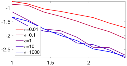
Refer to caption Refer to caption
d=2𝑑2d=2 d=5𝑑5d=5
Figure 8.9: Decay of 𝔼(log10(𝒲~p,ε(α^n,α^n)))𝔼subscript10subscript~𝒲𝑝𝜀subscript^𝛼𝑛superscriptsubscript^𝛼𝑛\mathbb{E}(\log_{10}(\tilde{\operatorname{\mathcal{W}}}_{p,\varepsilon}(\hat{\alpha}_{n},\hat{\alpha}_{n}^{\prime}))), for p=3/2𝑝32p=3/2 for various ε𝜀\varepsilon, as a function of log10(n)subscript10𝑛\log_{10}(n) where α𝛼\alpha is the same as in Figure 8.7.

The following proposition, whose proof can be found in (Ramdas et al., 2017), shows that this regularized divergence interpolates between the Wasserstein distance and the energy distance defined in Example 8.2.7.

Proposition 9.

One has

𝒲~p,ε(α,β)ε02𝒲p(α,β)and𝒲~p,ε(α,β)pε+αβED(𝒳,d)2,subscript~𝒲𝑝𝜀𝛼𝛽𝜀02subscript𝒲𝑝𝛼𝛽andsubscript~𝒲𝑝𝜀superscript𝛼𝛽𝑝𝜀superscriptsubscriptnorm𝛼𝛽ED𝒳𝑑2\tilde{\operatorname{\mathcal{W}}}_{p,\varepsilon}(\alpha,\beta)\overset{\varepsilon\rightarrow 0}{\longrightarrow}2\operatorname{\mathcal{W}}_{p}(\alpha,\beta)\quad\text{and}\quad\tilde{\operatorname{\mathcal{W}}}_{p,\varepsilon}(\alpha,\beta)^{p}\overset{\varepsilon\rightarrow+\infty}{\longrightarrow}\left\|\alpha-\beta\right\|_{\text{ED}(\mathcal{X},d)}^{2},

where ED(𝒳,d)\left\|\cdot\right\|_{\text{ED}(\mathcal{X},d)} is defined in (8.19).

Figure 8.9 shows numerically the impact of ε𝜀\varepsilon on the sample complexity rates. It is proved in Genevay et al. (2019), in the case of c(x,y)=xy2𝑐𝑥𝑦superscriptnorm𝑥𝑦2c(x,y)=\left\|x-y\right\|^{2} on 𝒳=d𝒳superscript𝑑\mathcal{X}=\mathbb{R}^{d}, that these rates interpolate between the ones of OT and MMD.

Chapter 9 Variational Wasserstein Problems

In data analysis, common divergences between probability measures (e.g. Euclidean, total variation, Hellinger, Kullback–Leibler) are often used to measure a fitting error or a loss in parameter estimation problems. Up to this chapter, we have made the case that the optimal transport geometry has a unique ability, not shared with other information divergences, to leverage physical ideas (mass displacement) and geometry (a ground cost between observations or bins) to compare measures. These two facts combined make it thus very tempting to use the Wasserstein distance as a loss function. This idea was recently explored for various applied problems. However, the main technical challenge associated with that idea lies in approximating and differentiating efficiently the Wasserstein distance. We start this chapter with a few motivating examples and show how the different numerical schemes presented in the first chapters of this book can be used to solve variational Wasserstein problems.

In image processing, the Wasserstein distance can be used as a loss to synthesize textures (Tartavel et al., 2016), to account for the discrepancy between statistics of synthesized and input examples. It is also used for image segmentation to account for statistical homogeneity of image regions (Swoboda and Schnörr, 2013; Rabin and Papadakis, 2015; Peyré et al., 2012; Ni et al., 2009; Schmitzer and Schnörr, 2013b; Li et al., 2018b). The Wasserstein distance is also a very natural fidelity term for inverse problems when the measurements are probability measures, for instance, image restoration (Lellmann et al., 2014), tomographic inversion (Abraham et al., 2017), density regularization (Burger et al., 2012), particle image velocimetry (Saumier et al., 2015), sparse recovery and compressed sensing (Indyk and Price, 2011), and seismic inversion (Métivier et al., 2016). Distances between measures (mostly kernel-based as shown in §8.2.2) are routinely used for shape matching (represented as measures over a lifted space, often called currents) in computational anatomy (Vaillant and Glaunès, 2005), but OT distances offer an interesting alternative (Feydy et al., 2017). To reduce the dimensionality of a dataset of histograms, Lee and Seung have shown that the nonnegative matrix factorization problem can be cast using the Kullback–Leibler divergence to quantify a reconstruction loss (Lee and Seung, 1999). When prior information is available on the geometry of the bins of those histograms, the Wasserstein distance can be used instead, with markedly different results (Sandler and Lindenbaum, 2011; Zen et al., 2014; Rolet et al., 2016).

All of these problems have in common that they require access to the gradients of Wasserstein distances, or approximations thereof. We start this section by presenting methods to approximate such gradients, then follow with three important applications that can be cast as variational Wasserstein problems.

9.1 Differentiating the Wasserstein Loss

In statistics, text processing or imaging, one must usually compare a probability distribution β𝛽\beta arising from measurements to a model, namely a parameterized family of distributions {αθ,θΘ}subscript𝛼𝜃𝜃Θ\{\alpha_{\theta},\theta\in\Theta\}, where ΘΘ\Theta is a subset of a Euclidean space. Such a comparison is done through a “loss” or a “fidelity” term, which is the Wasserstein distance in this section. In the simplest scenario, the computation of a suitable parameter θ𝜃\theta is obtained by minimizing directly

minθΘ(θ)=def.c(αθ,β).superscriptdef.𝜃Θ𝜃subscript𝑐subscript𝛼𝜃𝛽\underset{\theta\in\Theta}{\min}\;\mathcal{E}(\theta)\stackrel{{\scriptstyle\mbox{\tiny def.}}}{{=}}\mathcal{L}_{c}(\alpha_{\theta},\beta). (9.1)

Of course, one can consider more complicated problems: for instance, the barycenter problem described in §9.2 consists in a sum of such terms. However, most of these more advanced problems can be usually solved by adapting tools defined for the basic case above, either using the chain rule to compute explicitly derivatives or using automatic differentiation as advocated in §9.1.3.

Convexity.

The Wasserstein distance between two histograms or two densities is convex with respect to its two inputs, as shown by (2.20) and (2.24), respectively. Therefore, when the parameter θ𝜃\theta is itself a histogram, namely Θ=ΣnΘsubscriptΣ𝑛\Theta=\Sigma_{n} and αθ=θsubscript𝛼𝜃𝜃\alpha_{\theta}=\theta, or more generally when θ𝜃\theta describes K𝐾K weights in the simplex, Θ=ΣKΘsubscriptΣ𝐾\Theta=\Sigma_{K}, and αθ=i=1Kθiαisubscript𝛼𝜃superscriptsubscript𝑖1𝐾subscript𝜃𝑖subscript𝛼𝑖\alpha_{\theta}=\sum_{i=1}^{K}\theta_{i}\alpha_{i} is a convex combination of known atoms α1,,αKsubscript𝛼1subscript𝛼𝐾\alpha_{1},\dots,\alpha_{K} in ΣNsubscriptΣ𝑁\Sigma_{N}, Problem (9.1) remains convex (the first case corresponds to the barycenter problem, the second to one iteration of the dictionary learning problem with a Wasserstein loss (Rolet et al., 2016)). However, for more general parameterizations θαθmaps-to𝜃subscript𝛼𝜃\theta\mapsto\alpha_{\theta}, Problem (9.1) is in general not convex.

Simple cases.

For those simple cases where the Wasserstein distance has a closed form, such as univariate (see §2.30) or elliptically contoured (see §2.31) distributions, simple workarounds exist. They consist mostly in casting the Wasserstein distance as a simpler distance between suitable representations of these distributions (Euclidean on quantile functions for univariate measures, Bures metric for covariance matrices for elliptically contoured distributions of the same family) and solving Problem (9.1) directly on such representations.

In most cases, however, one has to resort to a careful discretization of αθsubscript𝛼𝜃\alpha_{\theta} to compute a local minimizer for Problem (9.1). Two approaches can be envisioned: Eulerian or Lagrangian. Figure 9.1 illustrates the difference between these two fundamental discretization schemes. At the risk of oversimplifying this argument, one may say that a Eulerian discretization is the most suitable when measures are supported on a low-dimensional space (as when dealing with shapes or color spaces), or for intrinsically discrete problems (such as those arising from string or text analysis). When applied to fitting problems where observations can take continuous values in high-dimensional spaces, a Lagrangian perspective is usually the only suitable choice.
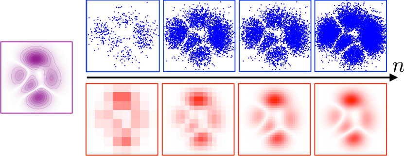
Refer to caption
Figure 9.1: Increasing fine discretization of a continuous distribution having a density (violet, left) using a Lagrangian representation 1niδxi1𝑛subscript𝑖subscript𝛿subscript𝑥𝑖\frac{1}{n}\sum_{i}\delta_{x_{i}} (blue, top) and an Eulerian representation iaiδxisubscript𝑖subscripta𝑖subscript𝛿subscript𝑥𝑖\sum_{i}\mathrm{\textbf{a}}_{i}\delta_{x_{i}} with xisubscript𝑥𝑖x_{i} representing cells on a grid of increasing size (red, bottom). The Eulerian perspective starts from a pixelated image down to one with such fine resolution that it almost matches the original density. Weights aisubscripta𝑖\mathrm{\textbf{a}}_{i} are directly proportional to each pixel-cell’s intensity.

9.1.1 Eulerian Discretization

A first way to discretize the problem is to suppose that both distributions β=j=1mbjδyj𝛽superscriptsubscript𝑗1𝑚subscriptb𝑗subscript𝛿subscript𝑦𝑗\beta=\sum_{j=1}^{m}\mathrm{\textbf{b}}_{j}\delta_{y_{j}} and αθ=i=1na(θ)iδxisubscript𝛼𝜃superscriptsubscript𝑖1𝑛asubscript𝜃𝑖subscript𝛿subscript𝑥𝑖\alpha_{\theta}=\sum_{i=1}^{n}\mathrm{\textbf{a}}(\theta)_{i}\delta_{x_{i}} are discrete distributions defined on fixed locations (xi)isubscriptsubscript𝑥𝑖𝑖(x_{i})_{i} and (yj)jsubscriptsubscript𝑦𝑗𝑗(y_{j})_{j}. Such locations might stand for cells dividing the entire space of observations in a grid, or a finite subset of points of interest in a continuous space (such as a family of vector embeddings for all words in a given dictionary (Kusner et al., 2015; Rolet et al., 2016)). The parameterized measure αθsubscript𝛼𝜃\alpha_{\theta} is in that case entirely represented through the weight vector a:θa(θ)Σn:amaps-to𝜃a𝜃subscriptΣ𝑛\mathrm{\textbf{a}}:\theta\mapsto\mathrm{\textbf{a}}(\theta)\in\Sigma_{n}, which, in practice, might be very sparse if the grid is large. This setting corresponds to the so-called class of Eulerian discretization methods. In its original form, the objective of Problem (9.1) is not differentiable. In order to obtain a smooth minimization problem, we use the entropic regularized OT and approximate (9.1) using

minθΘE(θ)=def.LCε(a(θ),b)whereCi,j=def.c(xi,yj).formulae-sequencesuperscriptdef.𝜃Θsubscript𝐸𝜃superscriptsubscriptLC𝜀a𝜃bwheresuperscriptdef.subscriptC𝑖𝑗𝑐subscript𝑥𝑖subscript𝑦𝑗\underset{\theta\in\Theta}{\min}\;\mathcal{E}_{E}(\theta)\stackrel{{\scriptstyle\mbox{\tiny def.}}}{{=}}\mathrm{L}_{\mathrm{\textbf{C}}}^{\varepsilon}(\mathrm{\textbf{a}}(\theta),\mathrm{\textbf{b}})\quad\text{where}\quad\mathrm{\textbf{C}}_{i,j}\stackrel{{\scriptstyle\mbox{\tiny def.}}}{{=}}c(x_{i},y_{j}).

We recall that Proposition 4.6 shows that the entropic loss function is differentiable and convex with respect to the input histograms, with gradient.

Proposition 9.1.1 (Derivative with respect to histograms).

For ε>0𝜀0\varepsilon>0, (a,b)LCε(a,b)maps-toabsuperscriptsubscriptLC𝜀ab(\mathrm{\textbf{a}},\mathrm{\textbf{b}})\mapsto\mathrm{L}_{\mathrm{\textbf{C}}}^{\varepsilon}(\mathrm{\textbf{a}},\mathrm{\textbf{b}}) is convex and differentiable. Its gradient reads

LCε(a,b)=(f,g),superscriptsubscriptLC𝜀abfg\nabla\mathrm{L}_{\mathrm{\textbf{C}}}^{\varepsilon}(\mathrm{\textbf{a}},\mathrm{\textbf{b}})=(\mathrm{\textbf{f}},\mathrm{\textbf{g}}), (9.2)

where (f,g)fg(\mathrm{\textbf{f}},\mathrm{\textbf{g}}) is the unique solution to (4.30), centered such that ifi=jgj=0subscript𝑖subscriptf𝑖subscript𝑗subscriptg𝑗0\sum_{i}\mathrm{\textbf{f}}_{i}=\sum_{j}\mathrm{\textbf{g}}_{j}=0. For ε=0𝜀0\varepsilon=0, this formula defines the elements of the sub-differential of LCεsuperscriptsubscriptLC𝜀\mathrm{L}_{\mathrm{\textbf{C}}}^{\varepsilon}, and the function is differentiable if they are unique.

The zero mean condition on (f,g)fg(\mathrm{\textbf{f}},\mathrm{\textbf{g}}) is important when using gradient descent to guarantee conservation of mass. Using the chain rule, one thus obtains that Esubscript𝐸\mathcal{E}_{E} is smooth and that its gradient is

E(θ)=[a(θ)](f),subscript𝐸𝜃superscriptdelimited-[]a𝜃topf\nabla\mathcal{E}_{E}(\theta)=[\partial\mathrm{\textbf{a}}(\theta)]^{\top}(\mathrm{\textbf{f}}\,), (9.3)

where a(θ)n×dim(Θ)a𝜃superscript𝑛dimΘ\partial\mathrm{\textbf{a}}(\theta)\in\mathbb{R}^{n\times\text{dim}(\Theta)} is the Jacobian (differential) of the map a(θ)a𝜃\mathrm{\textbf{a}}(\theta), and where fnfsuperscript𝑛\mathrm{\textbf{f}}\in\mathbb{R}^{n} is the dual potential vector associated to the dual entropic OT (4.30) between a(θ)a𝜃\mathrm{\textbf{a}}(\theta) and b for the cost matrix C (which is fixed in a Eulerian setting, and in particular independent of θ𝜃\theta). This result can be used to minimize locally Esubscript𝐸\mathcal{E}_{E} through gradient descent.

9.1.2 Lagrangian Discretization

A different approach consists in using instead fixed (typically uniform) weights and approximating an input measure α𝛼\alpha as an empirical measure αθ=1niδx(θ)isubscript𝛼𝜃1𝑛subscript𝑖subscript𝛿𝑥subscript𝜃𝑖\alpha_{\theta}=\frac{1}{n}\sum_{i}\delta_{x(\theta)_{i}} for a point-cloud parameterization map x:θx(θ)=(x(θ)i)i=1n𝒳n:𝑥maps-to𝜃𝑥𝜃superscriptsubscript𝑥subscript𝜃𝑖𝑖1𝑛superscript𝒳𝑛x:\theta\mapsto x(\theta)=(x(\theta)_{i})_{i=1}^{n}\in\mathcal{X}^{n}, where we assume here that 𝒳𝒳\mathcal{X} is Euclidean. Problem (9.1) is thus approximated as

min𝜃L(θ)=def.LC(x(θ))ε(𝟙n/n,b)whereC(x)i,j=def.c(x(θ)i,yj).formulae-sequencesuperscriptdef.𝜃subscript𝐿𝜃superscriptsubscriptLC𝑥𝜃𝜀subscriptdouble-struck-𝟙𝑛𝑛bwheresuperscriptdef.Csubscript𝑥𝑖𝑗𝑐𝑥subscript𝜃𝑖subscript𝑦𝑗\underset{\theta}{\min}\;\mathcal{E}_{L}(\theta)\stackrel{{\scriptstyle\mbox{\tiny def.}}}{{=}}\mathrm{L}_{\mathrm{\textbf{C}}(x(\theta))}^{\varepsilon}(\mathbb{1}_{n}/n,\mathrm{\textbf{b}})\quad\text{where}\quad\mathrm{\textbf{C}}(x)_{i,j}\stackrel{{\scriptstyle\mbox{\tiny def.}}}{{=}}c(x(\theta)_{i},y_{j}). (9.4)

Note that here the cost matrix C(x(θ))C𝑥𝜃\mathrm{\textbf{C}}(x(\theta)) now depends on θ𝜃\theta since the support of αθsubscript𝛼𝜃\alpha_{\theta} changes with θ𝜃\theta. The following proposition shows that the entropic OT loss is a smooth function of the cost matrix and gives the expression of its gradient.

Proposition 9.1.2 (Derivative with respect to the cost).

For fixed input histograms (a,b)ab(\mathrm{\textbf{a}},\mathrm{\textbf{b}}), for ε>0𝜀0\varepsilon>0, the mapping C(C)=def.LCε(a,b)maps-toCCsuperscriptdef.superscriptsubscriptLC𝜀ab\mathrm{\textbf{C}}\mapsto\mathcal{R}(\mathrm{\textbf{C}})\stackrel{{\scriptstyle\mbox{\tiny def.}}}{{=}}\mathrm{L}_{\mathrm{\textbf{C}}}^{\varepsilon}(\mathrm{\textbf{a}},\mathrm{\textbf{b}}) is concave and smooth, and

(C)=P,CP\nabla\mathcal{R}(\mathrm{\textbf{C}})=\mathrm{\textbf{P}}, (9.5)

where P is the unique optimal solution of (4.2). For ε=0𝜀0\varepsilon=0, this formula defines the set of upper gradients.

Assuming (𝒳,𝒴)𝒳𝒴(\mathcal{X},\mathcal{Y}) are convex subsets of dsuperscript𝑑\mathbb{R}^{d}, for discrete measures (α,β)𝛼𝛽(\alpha,\beta) of the form (2.3), one obtains using the chain rule that x=(xi)i=1n𝒳n(x)=def.LC(x)(𝟙n/n,b)𝑥superscriptsubscriptsubscript𝑥𝑖𝑖1𝑛superscript𝒳𝑛maps-to𝑥superscriptdef.subscriptLC𝑥subscriptdouble-struck-𝟙𝑛𝑛bx=(x_{i})_{i=1}^{n}\in\mathcal{X}^{n}\mapsto\mathcal{F}(x)\stackrel{{\scriptstyle\mbox{\tiny def.}}}{{=}}\mathrm{L}_{\mathrm{\textbf{C}}(x)}(\mathbb{1}_{n}/n,\mathrm{\textbf{b}}) is smooth and that

(x)=(j=1mPi,j1c(xi,yj))i=1n𝒳n,𝑥superscriptsubscriptsuperscriptsubscript𝑗1𝑚subscriptP𝑖𝑗subscript1𝑐subscript𝑥𝑖subscript𝑦𝑗𝑖1𝑛superscript𝒳𝑛\nabla\mathcal{F}(x)=\left(\sum_{j=1}^{m}\mathrm{\textbf{P}}_{i,j}\nabla_{1}c(x_{i},y_{j})\right)_{i=1}^{n}\in\mathcal{X}^{n}, (9.6)

where 1csubscript1𝑐\nabla_{1}c is the gradient with respect to the first variable. For instance, for 𝒳=𝒴=d𝒳𝒴superscript𝑑\mathcal{X}=\mathcal{Y}=\mathbb{R}^{d}, for c(s,t)=st2𝑐𝑠𝑡superscriptnorm𝑠𝑡2c(s,t)=\left\|s-t\right\|^{2} on 𝒳=𝒴=d𝒳𝒴superscript𝑑\mathcal{X}=\mathcal{Y}=\mathbb{R}^{d}, one has

(x)=2(aixij=1mPi,jyj)i=1n,𝑥2superscriptsubscriptsubscripta𝑖subscript𝑥𝑖superscriptsubscript𝑗1𝑚subscriptP𝑖𝑗subscript𝑦𝑗𝑖1𝑛\nabla\mathcal{F}(x)=2\left(\mathrm{\textbf{a}}_{i}x_{i}-\sum_{j=1}^{m}\mathrm{\textbf{P}}_{i,j}y_{j}\right)_{i=1}^{n}, (9.7)

where ai=1/nsubscripta𝑖1𝑛\mathrm{\textbf{a}}_{i}=1/n here. Note that, up to a constant, this gradient is IdTId𝑇\mathrm{Id}-T, where T𝑇T is the barycentric projection defined in (4.19). Using the chain rule, one thus obtains that the Lagrangian discretized problem (9.4) is smooth and its gradient is

L(θ)=[x(θ)]((x(θ))),subscript𝐿𝜃superscriptdelimited-[]𝑥𝜃top𝑥𝜃\nabla\mathcal{E}_{L}(\theta)=[\partial x(\theta)]^{\top}(\nabla\mathcal{F}(x(\theta))), (9.8)

where x(θ)dim(Θ)×(nd)𝑥𝜃superscriptdimΘ𝑛𝑑\partial x(\theta)\in\mathbb{R}^{\text{dim}(\Theta)\times(nd)} is the Jacobian of the map x(θ)𝑥𝜃x(\theta) and where \nabla\mathcal{F} is implemented as in (9.6) or (9.7) using for P the optimal coupling matrix between αθsubscript𝛼𝜃\alpha_{\theta} and β𝛽\beta. One can thus implement a gradient descent to compute a local minimizer of Lsubscript𝐿\mathcal{E}_{L}, as used, for instance, in (Cuturi and Doucet, 2014).

9.1.3 Automatic Differentiation

The difficulty when applying formulas (9.3) and (9.8) is that one needs to compute the exact optimal solutions f or P for these formulas to be valid, which can only be achieved with acceptable precision using a very large number of Sinkhorn iterates. In challenging situations in which the size and the quantity of histograms to be compared are large, the computational budget to compute a single Wasserstein distance is usually limited, therefore allowing only for a few Sinkhorn iterations. In that case, and rather than approximating the gradient (4.30) using the value obtained at a given iterate, it is usually better to differentiate directly the output of Sinkhorn’s algorithm, using reverse mode automatic differentiation. This corresponds to using the “algorithmic” Sinkhorn divergences as introduced in (4.48), rather than the quantity LCεsuperscriptsubscriptLC𝜀\mathrm{L}_{\mathrm{\textbf{C}}}^{\varepsilon} in (4.2) which incorporates the entropy of the regularized optimal transport, and differentiating it directly as a composition of simple maps using the inputs, either the histogram in the Eulerian case or the cost matrix in the Lagrangian cases. Using definitions introduced in §4.5, this is equivalent to differentiating

𝔇C(L)(a(θ),b) or 𝔇C(x(θ))(L)(a,b)superscriptsubscript𝔇C𝐿a𝜃b or superscriptsubscript𝔇C𝑥𝜃𝐿ab\mathfrak{D}_{\mathrm{\textbf{C}}}^{(L)}(\mathrm{\textbf{a}}(\theta),\mathrm{\textbf{b}})\quad\text{ or }\quad\mathfrak{D}_{\mathrm{\textbf{C}}(x(\theta))}^{(L)}(\mathrm{\textbf{a}},\mathrm{\textbf{b}})

with respect to θ𝜃\theta, in, respectively, the Eulerian and the Lagrangian cases for L𝐿L large enough.

The cost for computing the gradient of functionals involving Sinkhorn divergences is the same as that of computation of the functional itself; see, for instance, (Bonneel et al., 2016; Genevay et al., 2018) for some applications of this approach. We also refer to (Adams and Zemel, 2011) for an early work on differentiating Sinkhorn iterations with respect to the cost matrix (as done in the Lagrangian framework), with applications to learning rankings. Further details on automatic differentiation can be found in (Griewank and Walther, 2008; Rall, 1981; Neidinger, 2010), in particular on the “reverse mode,” which is the fastest way to compute gradients. In terms of implementation, all recent deep-learning Python frameworks feature state-of-the-art reverse-mode differentiation and support for GPU/TPU computations (Al-Rfou et al., 2016; Abadi et al., 2016; Pytorch, 2017), they should be adopted for any large-scale application of Sinkhorn losses. We strongly encourage the use of such automatic differentiation techniques, since they have the same complexity as computing (9.3) and (9.8), these formulas being mostly useful to obtain a theoretical understanding of what automatic differentation is computing. The only downside is that reverse mode automatic differentation is memory intensive (the memory grows proportionally with the number of iterations). There exist, however, subsampling strategies that mitigate this problem (Griewank, 1992).

9.2 Wasserstein Barycenters, Clustering and Dictionary Learning

A basic problem in unsupervised learning is to compute the “mean” or “barycenter” of several data points. A classical way to define such a weighted mean of points (xs)s=1S𝒳Ssuperscriptsubscriptsubscript𝑥𝑠𝑠1𝑆superscript𝒳𝑆(x_{s})_{s=1}^{S}\in\mathcal{X}^{S} living in a metric space (𝒳,d)𝒳𝑑(\mathcal{X},d) (where d𝑑d is a distance or more generally a divergence) is by solving a variational problem

minx𝒳s=1Sλsd(x,xs)p𝑥𝒳superscriptsubscript𝑠1𝑆subscript𝜆𝑠𝑑superscript𝑥subscript𝑥𝑠𝑝\underset{x\in\mathcal{X}}{\min}\;\sum_{s=1}^{S}\lambda_{s}d(x,x_{s})^{p} (9.9)

for a given family of weights (λs)sΣSsubscriptsubscript𝜆𝑠𝑠subscriptΣ𝑆(\lambda_{s})_{s}\in\Sigma_{S}, where p𝑝p is often set to p=2𝑝2p=2. When 𝒳=d𝒳superscript𝑑\mathcal{X}=\mathbb{R}^{d} and d(x,y)=xy2𝑑𝑥𝑦subscriptnorm𝑥𝑦2d(x,y)=\left\|x-y\right\|_{2}, this leads to the usual definition of the linear average x=sλsxs𝑥subscript𝑠subscript𝜆𝑠subscript𝑥𝑠x=\sum_{s}\lambda_{s}x_{s} for p=2𝑝2p=2 and the more evolved median point when p=1𝑝1p=1. One can retrieve various notions of means (e.g. harmonic or geometric means over 𝒳=+𝒳subscript\mathcal{X}=\mathbb{R}_{+}) using this formalism. This process is often referred to as the “Fréchet” or “Karcher” mean (see Karcher (2014) for a historical account). For a generic distance d𝑑d, Problem (9.9) is usually a difficult nonconvex optimization problem. Fortunately, in the case of optimal transport distances, the problem can be formulated as a convex program for which existence can be proved and efficient numerical schemes exist.

Fréchet means over the Wasserstein space.

Given input histogram {bs}s=1Ssuperscriptsubscriptsubscriptb𝑠𝑠1𝑆\{\mathrm{\textbf{b}}_{s}\}_{s=1}^{S}, where bsΣnssubscript𝑏𝑠subscriptΣsubscript𝑛𝑠b_{s}\in\Sigma_{n_{s}}, and weights λΣS𝜆subscriptΣ𝑆\lambda\in\Sigma_{S}, a Wasserstein barycenter is computed by minimizing

minaΣns=1SλsLCs(a,bs),asubscriptΣ𝑛superscriptsubscript𝑠1𝑆subscript𝜆𝑠subscriptLsubscriptC𝑠asubscriptb𝑠\underset{\mathrm{\textbf{a}}\in\Sigma_{n}}{\min}\;\sum_{s=1}^{S}\lambda_{s}\mathrm{L}_{\mathrm{\textbf{C}}_{s}}(\mathrm{\textbf{a}},\mathrm{\textbf{b}}_{s}), (9.10)

where the cost matrices Csn×nssubscriptC𝑠superscript𝑛subscript𝑛𝑠\mathrm{\textbf{C}}_{s}\in\mathbb{R}^{n\times n_{s}} need to be specified. A typical setup is “Eulerian,” so that all the barycenters are defined on the same grid, ns=nsubscript𝑛𝑠𝑛n_{s}=n, Cs=C=DpsubscriptC𝑠CsuperscriptD𝑝\mathrm{\textbf{C}}_{s}=\mathrm{\textbf{C}}=\mathrm{\textbf{D}}^{p} is set to be a distance matrix, to solve

minaΣns=1SλsWpp(a,bs).asubscriptΣ𝑛superscriptsubscript𝑠1𝑆subscript𝜆𝑠superscriptsubscriptW𝑝𝑝asubscriptb𝑠\underset{\mathrm{\textbf{a}}\in\Sigma_{n}}{\min}\;\sum_{s=1}^{S}\lambda_{s}\operatorname{\mathrm{W}}_{p}^{p}(\mathrm{\textbf{a}},\mathrm{\textbf{b}}_{s}).

The barycenter problem (9.10) was introduced in a more general form involving arbitrary measures in Agueh and Carlier (2011) following earlier ideas of Carlier and Ekeland (2010). That presentation is deferred to Remark 1. The barycenter problem for histograms (9.10) is in fact a linear program, since one can look for the S𝑆S couplings (Ps)ssubscriptsubscriptP𝑠𝑠(\mathrm{\textbf{P}}_{s})_{s} between each input and the barycenter itself, which by construction must be constrained to share the same row marginal,

minaΣn,(Psn×ns)s{s=1SλsPs,Cs:s,Ps𝟙ns=a,Ps𝟙n=bs}.asubscriptΣ𝑛subscriptsubscriptP𝑠superscript𝑛subscript𝑛𝑠𝑠conditional-setsuperscriptsubscript𝑠1𝑆subscript𝜆𝑠subscriptP𝑠subscriptC𝑠formulae-sequencefor-all𝑠superscriptsubscriptP𝑠topsubscriptdouble-struck-𝟙subscript𝑛𝑠asuperscriptsubscriptP𝑠topsubscriptdouble-struck-𝟙𝑛subscriptb𝑠\underset{\mathrm{\textbf{a}}\in\Sigma_{n},(\mathrm{\textbf{P}}_{s}\in\mathbb{R}^{n\times n_{s}})_{s}}{\min}\;\left\{\sum_{s=1}^{S}\lambda_{s}\langle\mathrm{\textbf{P}}_{s},\,\mathrm{\textbf{C}}_{s}\rangle\;:\;\forall\,s,\mathrm{\textbf{P}}_{s}^{\top}\mathbb{1}_{n_{s}}=\mathrm{\textbf{a}},\mathrm{\textbf{P}}_{s}^{\top}\mathbb{1}_{n}=\mathrm{\textbf{b}}_{s}\right\}.

Although this problem is an LP, its scale forbids the use of generic solvers for medium-scale problems. One can resort to using first order methods such as subgradient descent on the dual (Carlier et al., 2015).

Remark 1 (Barycenter of arbitrary measures).
Given a set of input measure (βs)ssubscriptsubscript𝛽𝑠𝑠(\beta_{s})_{s} defined on some space 𝒳𝒳\mathcal{X}, the barycenter problem becomes minα+1(𝒳)s=1Sλsc(α,βs).𝛼superscriptsubscript1𝒳superscriptsubscript𝑠1𝑆subscript𝜆𝑠subscript𝑐𝛼subscript𝛽𝑠\underset{\alpha\in\mathcal{M}_{+}^{1}(\mathcal{X})}{\min}\;\sum_{s=1}^{S}\lambda_{s}\mathcal{L}_{c}(\alpha,\beta_{s}). (9.11) In the case where 𝒳=d𝒳superscript𝑑\mathcal{X}=\mathbb{R}^{d} and c(x,y)=xy2𝑐𝑥𝑦superscriptnorm𝑥𝑦2c(x,y)=\left\|x-y\right\|^{2}Agueh and Carlier (2011) show that if one of the input measures has a density, then this barycenter is unique. Problem (9.11) can be viewed as a generalization of the problem of computing barycenters of points (xs)s=1S𝒳Ssuperscriptsubscriptsubscript𝑥𝑠𝑠1𝑆superscript𝒳𝑆(x_{s})_{s=1}^{S}\in\mathcal{X}^{S} to arbitrary measures. Indeed, if βs=δxssubscript𝛽𝑠subscript𝛿subscript𝑥𝑠\beta_{s}=\delta_{x_{s}} is a single Dirac mass, then a solution to (9.11) is δxsubscript𝛿superscript𝑥\delta_{x^{\star}}, where xsuperscript𝑥x^{\star} is a Fréchet mean solving (9.9). Note that for c(x,y)=xy2𝑐𝑥𝑦superscriptnorm𝑥𝑦2c(x,y)=\left\|x-y\right\|^{2}, the mean of the barycenter αsuperscript𝛼\alpha^{\star} is necessarily the barycenter of the mean, i.e. 𝒳xdα(x)=sλs𝒳xdαs(x),subscript𝒳𝑥differential-dsuperscript𝛼𝑥subscript𝑠subscript𝜆𝑠subscript𝒳𝑥differential-dsubscript𝛼𝑠𝑥\int_{\mathcal{X}}x\mathrm{d}\alpha^{\star}(x)=\sum_{s}\lambda_{s}\int_{\mathcal{X}}x\mathrm{d}\alpha_{s}(x), and the support of αsuperscript𝛼\alpha^{\star} is located in the convex hull of the supports of the (αs)ssubscriptsubscript𝛼𝑠𝑠(\alpha_{s})_{s}. The consistency of the approximation of the infinite-dimensional optimization (9.11) when approximating the input distribution using discrete ones (and thus solving (9.10) in place) is studied in Carlier et al. (2015). Let us also note that it is possible to recast (9.11) as a multimarginal OT problem; see Remark 2.
Remark 2 (k𝑘k-means as a Wasserstein variational problem).
When the family of input measures (βs)ssubscriptsubscript𝛽𝑠𝑠(\beta_{s})_{s} is limited to but one measure β𝛽\beta, this measure is supported on a discrete finite subset of 𝒳=d𝒳superscript𝑑\mathcal{X}=\mathbb{R}^{d}, and the cost is the squared Euclidean distance, then one can show that the barycenter problem minαk1(𝒳)c(α,β),𝛼superscriptsubscript𝑘1𝒳subscript𝑐𝛼𝛽\underset{\alpha\in\mathcal{M}_{k}^{1}(\mathcal{X})}{\min}\;\mathcal{L}_{c}(\alpha,\beta), (9.12) where α𝛼\alpha is constrained to be a discrete measure with a finite support of size up to k𝑘k, is equivalent to the usual k𝑘k-means problem taking β𝛽\beta. Indeed, one can easily show that the centroids output by the k𝑘k-means problem correspond to the support of the solution α𝛼\alpha and that its weights correspond to the fraction of points in β𝛽\beta assigned to each centroid. One can show that approximating csubscript𝑐\mathcal{L}_{c} using entropic regularization results in smoothed out assignments that appear in soft-clustering variants of k𝑘k-means, such as mixtures of Gaussians (Dessein et al., 2017).
Remark 3 (Distribution of distributions and consistency).
It is possible to generalize (9.11) to a possibly infinite collection of measures. This problem is described by considering a probability distribution M𝑀M over the space +1(𝒳)superscriptsubscript1𝒳\mathcal{M}_{+}^{1}(\mathcal{X}) of probability distributions, i.e. M+1(+1(𝒳))𝑀superscriptsubscript1superscriptsubscript1𝒳M\in\mathcal{M}_{+}^{1}(\mathcal{M}_{+}^{1}(\mathcal{X})). A barycenter is then a solution of minα+1(𝒳)𝔼M(c(α,β))=+1(𝒳)c(α,β)dM(β),𝛼superscriptsubscript1𝒳subscript𝔼𝑀subscript𝑐𝛼𝛽subscriptsuperscriptsubscript1𝒳subscript𝑐𝛼𝛽differential-d𝑀𝛽\underset{\alpha\in\mathcal{M}_{+}^{1}(\mathcal{X})}{\min}\;\mathbb{E}_{M}(\mathcal{L}_{c}(\alpha,\beta))=\int_{\mathcal{M}_{+}^{1}(\mathcal{X})}\mathcal{L}_{c}(\alpha,\beta)\mathrm{d}M(\beta), (9.13) where β𝛽\beta is a random measure distributed according to M𝑀M. Drawing uniformly at random a finite number S𝑆S of input measures (βs)s=1Ssuperscriptsubscriptsubscript𝛽𝑠𝑠1𝑆(\beta_{s})_{s=1}^{S} according to M𝑀M, one can then define β^Ssubscript^𝛽𝑆\hat{\beta}_{S} as being a solution of (9.11) for uniform weights λs=1/Ssubscript𝜆𝑠1𝑆\lambda_{s}=1/S (note that here β^Ssubscript^𝛽𝑆\hat{\beta}_{S} is itself a random measure). Problem (9.11) corresponds to the special case of a “discrete” measure M=sλsδβs𝑀subscript𝑠subscript𝜆𝑠subscript𝛿subscript𝛽𝑠M=\sum_{s}\lambda_{s}\delta_{\beta_{s}}. The convergence (in expectation or with high probability) of c(β^S,α)subscript𝑐subscript^𝛽𝑆𝛼\mathcal{L}_{c}(\hat{\beta}_{S},\alpha) to zero (where α𝛼\alpha is the unique solution to (9.13)) corresponds to the consistency of the barycenters, and is proved in (Bigot and Klein, 2012a; Le Gouic and Loubes, 2016; Bigot and Klein, 2012b). This can be interpreted as a law of large numbers over the Wasserstein space. The extension of this result to a central limit theorem is an important problem; see (Panaretos and Zemel, 2016) and (Agueh and Carlier, 2017) for recent formulations of that problem and solutions in particular cases (1-D distributions and Gaussian measures).
Remark 4 (Fixed-point map).
When dealing with the Euclidean space 𝒳=d𝒳superscript𝑑\mathcal{X}=\mathbb{R}^{d} with ground cost c(x,y)=xy2𝑐𝑥𝑦superscriptnorm𝑥𝑦2c(x,y)=\left\|x-y\right\|^{2}, it is possible to study the barycenter problem using transportation maps. Indeed, if α𝛼\alpha has a density, according to Remark 2.24, one can define optimal transportation maps Tssubscript𝑇𝑠T_{s} between α𝛼\alpha and αssubscript𝛼𝑠\alpha_{s}, in particular such that Ts,α=αssubscript𝑇𝑠𝛼subscript𝛼𝑠T_{s,\sharp}\alpha=\alpha_{s}. The average map T(α)=def.s=1SλsTssuperscriptdef.superscript𝑇𝛼superscriptsubscript𝑠1𝑆subscript𝜆𝑠subscript𝑇𝑠T^{(\alpha)}\stackrel{{\scriptstyle\mbox{\tiny def.}}}{{=}}\sum_{s=1}^{S}\lambda_{s}T_{s} (the notation above makes explicit the dependence of this map on α𝛼\alpha) is itself an optimal map between α𝛼\alpha and T(α)αsubscriptsuperscript𝑇𝛼𝛼T^{(\alpha)}_{\sharp}\alpha (a positive combination of optimal maps is equal by Brenier’s theorem, Remark 2.24, to the sum of gradients of convex functions, equal to the gradient of a sum of convex functions, and therefore optimal by Brenier’s theorem again). As shown in (Agueh and Carlier, 2011), first order optimality conditions of the barycenter problem (9.13) actually read T(α)=𝕀dsuperscript𝑇superscript𝛼subscript𝕀superscript𝑑T^{(\alpha^{\star})}=\mathbb{I}_{\mathbb{R}^{d}} (the identity map) at the optimal measure αsuperscript𝛼\alpha^{\star} (the barycenter), and it is shown in (Álvarez-Esteban et al., 2016) that the barycenter αsuperscript𝛼\alpha^{\star} is the unique (under regularity conditions clarified in (Zemel and Panaretos, 2018, Theo. 2)) to the fixed-point equation G(α)=αwhereG(α)=def.T(α)α,formulae-sequence𝐺𝛼𝛼wheresuperscriptdef.𝐺𝛼subscriptsuperscript𝑇𝛼𝛼G(\alpha)=\alpha\quad\text{where}\quad G(\alpha)\stackrel{{\scriptstyle\mbox{\tiny def.}}}{{=}}T^{(\alpha)}_{\sharp}\alpha, (9.14) Under mild conditions on the input measures, Álvarez-Esteban et al. (2016) and Zemel and Panaretos (2018) have shown that αG(α)maps-to𝛼𝐺𝛼\alpha\mapsto G(\alpha) strictly decreases the objective function of (9.13) if α𝛼\alpha is not the barycenter and that the fixed-point iterations α(+1)=def.G(α())superscriptdef.superscript𝛼1𝐺superscript𝛼\alpha^{(\ell+1)}\stackrel{{\scriptstyle\mbox{\tiny def.}}}{{=}}G(\alpha^{(\ell)}) converge to the barycenter αsuperscript𝛼\alpha^{\star}. This fixed point algorithm can be used in cases where the optimal transportation maps are known in closed form (e.g. for Gaussians). Adapting this algorithm for empirical measures of the same size results in computing optimal assignments in place of Monge maps. For more general discrete measures of arbitrary size the scheme can also be adapted (Cuturi and Doucet, 2014) using barycentric projections (4.19).
Special cases.

In general, solving (9.10) or (9.11) is not straightforward, but there exist some special cases for which solutions are explicit or simple.

Remark 5 (Barycenter of Gaussians).
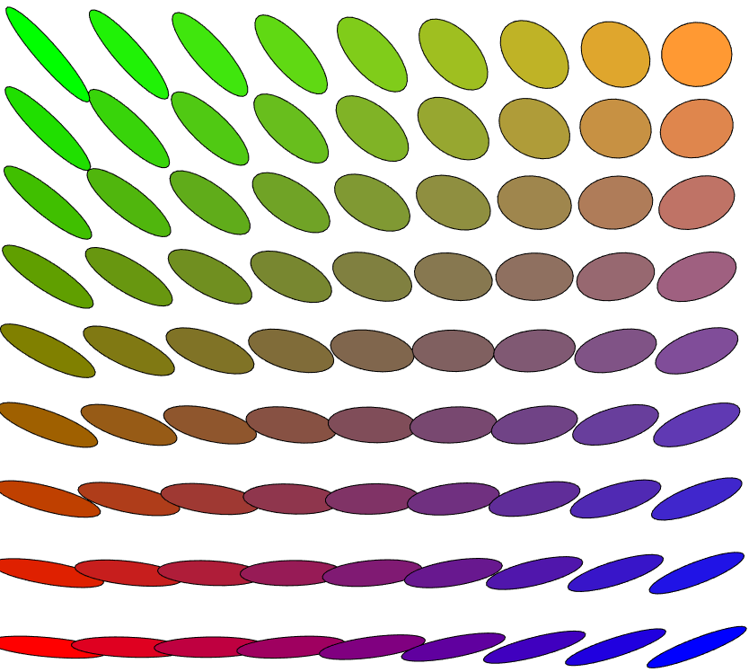
It is shown in (Agueh and Carlier, 2011) that the barycenter of Gaussians distributions αs=𝒩(𝐦s,𝚺s)subscript𝛼𝑠𝒩subscript𝐦𝑠subscript𝚺𝑠\alpha_{s}=\mathcal{N}(\mathbf{m}_{s},\mathbf{\Sigma}_{s}), for the squared Euclidean cost c(x,y)=xy2𝑐𝑥𝑦superscriptnorm𝑥𝑦2c(x,y)=\left\|x-y\right\|^{2}, is itself a Gaussian 𝒩(𝐦,𝚺)𝒩superscript𝐦superscript𝚺\mathcal{N}(\mathbf{m}^{\star},\mathbf{\Sigma}^{\star}). Making use of (2.41), one sees that the barycenter mean is the mean of the inputs 𝐦=sλs𝐦ssuperscript𝐦subscript𝑠subscript𝜆𝑠subscript𝐦𝑠\mathbf{m}^{\star}=\sum_{s}\lambda_{s}\mathbf{m}_{s} while the covariance minimizes min𝚺sλs(𝚺,𝚺s)2,𝚺subscript𝑠subscript𝜆𝑠superscript𝚺subscript𝚺𝑠2\underset{\mathbf{\Sigma}}{\min}\;\sum_{s}\lambda_{s}\mathcal{B}(\mathbf{\Sigma},\mathbf{\Sigma}_{s})^{2}, where \mathcal{B} is the Bure metric (2.42). As studied in (Agueh and Carlier, 2011), the first order optimality condition of this convex problem shows that 𝚺superscript𝚺\mathbf{\Sigma}^{\star} is the unique positive definite fixed point of the map 𝚺=Ψ(𝚺)whereΨ(𝚺)=def.sλs(𝚺12𝚺s𝚺12)12,formulae-sequencesuperscript𝚺Ψsuperscript𝚺wheresuperscriptdef.Ψ𝚺subscript𝑠subscript𝜆𝑠superscriptsuperscript𝚺12subscript𝚺𝑠superscript𝚺1212\mathbf{\Sigma}^{\star}=\Psi(\mathbf{\Sigma}^{\star})\quad\text{where}\quad\Psi(\mathbf{\Sigma})\stackrel{{\scriptstyle\mbox{\tiny def.}}}{{=}}\sum_{s}\lambda_{s}(\mathbf{\Sigma}^{\frac{1}{2}}\mathbf{\Sigma}_{s}\mathbf{\Sigma}^{\frac{1}{2}})^{\frac{1}{2}}, where 𝚺12superscript𝚺12\mathbf{\Sigma}^{\frac{1}{2}} is the square root of positive semidefinite matrices. This result was known from (Knott and Smith, 1994; Rüschendorf and Uckelmann, 2002) and is proved in (Agueh and Carlier, 2011). While ΨΨ\Psi is not strictly contracting, iterating this fixed-point map, i.e. defining 𝚺(+1)=def.Ψ(𝚺())superscriptdef.superscript𝚺1Ψsuperscript𝚺\mathbf{\Sigma}^{(\ell+1)}\stackrel{{\scriptstyle\mbox{\tiny def.}}}{{=}}\Psi(\mathbf{\Sigma}^{(\ell)}) converges in practice to the solution 𝚺superscript𝚺\mathbf{\Sigma}^{\star}. This method has been applied to texture synthesis in (Xia et al., 2014). Álvarez-Esteban et al. (2016) have also proposed to use an alternative map Ψ¯(𝚺)=def.𝚺12(sλs(𝚺12𝚺s𝚺12)12)2𝚺12superscriptdef.¯Ψ𝚺superscript𝚺12superscriptsubscript𝑠subscript𝜆𝑠superscriptsuperscript𝚺12subscript𝚺𝑠superscript𝚺12122superscript𝚺12\bar{\Psi}(\mathbf{\Sigma})\stackrel{{\scriptstyle\mbox{\tiny def.}}}{{=}}\mathbf{\Sigma}^{-\frac{1}{2}}\Big{(}\sum_{s}\lambda_{s}(\mathbf{\Sigma}^{\frac{1}{2}}\mathbf{\Sigma}_{s}\mathbf{\Sigma}^{\frac{1}{2}})^{\frac{1}{2}}\Big{)}^{2}\mathbf{\Sigma}^{-\frac{1}{2}} for which the iterations 𝚺(+1)=def.Ψ¯(𝚺())superscriptdef.superscript𝚺1¯Ψsuperscript𝚺\mathbf{\Sigma}^{(\ell+1)}\stackrel{{\scriptstyle\mbox{\tiny def.}}}{{=}}\bar{\Psi}(\mathbf{\Sigma}^{(\ell)}) converge. This is because the fixed-point map G𝐺G defined in (9.14) preserves Gaussian distributions, and in fact, G(𝒩(𝐦,𝚺))=𝒩(𝐦,Ψ¯(𝚺)).𝐺𝒩𝐦𝚺𝒩superscript𝐦¯Ψ𝚺G(\mathcal{N}(\mathbf{m},\mathbf{\Sigma}))=\mathcal{N}(\mathbf{m}^{\star},\bar{\Psi}(\mathbf{\Sigma})). Figure 9.2 shows two examples of computations of barycenters between four 2-D Gaussians.
Refer to caption Refer to caption
Figure 9.2: Barycenters between four Gaussian distributions in 2-D. Each Gaussian is displayed using an ellipse aligned with the principal axes of the covariance, and with elongations proportional to the corresponding eigenvalues.
Remark 6 (1-D cases).
For 1-D distributions, the 𝒲psubscript𝒲𝑝\operatorname{\mathcal{W}}_{p} barycenter can be computed almost in closed form using the fact that the transport is the monotone rearrangement, as detailed in Remark 2.30. The simplest case is for empirical measures with n𝑛n points, i.e. βs=1ni=1nδys,isubscript𝛽𝑠1𝑛superscriptsubscript𝑖1𝑛subscript𝛿subscript𝑦𝑠𝑖\beta_{s}=\frac{1}{n}\sum_{i=1}^{n}\delta_{y_{s,i}}, where the points are assumed to be sorted ys,1ys,2subscript𝑦𝑠1subscript𝑦𝑠2y_{s,1}\leq y_{s,2}\leq\ldots. Using (2.33) the barycenter αλsubscript𝛼𝜆\alpha_{\lambda} is also an empirical measure on n𝑛n points αλ=1ni=1nδxλ,iwherexλ,i=Aλ(xs,i)s,formulae-sequencesubscript𝛼𝜆1𝑛superscriptsubscript𝑖1𝑛subscript𝛿subscript𝑥𝜆𝑖wheresubscript𝑥𝜆𝑖subscript𝐴𝜆subscriptsubscript𝑥𝑠𝑖𝑠\alpha_{\lambda}=\frac{1}{n}\sum_{i=1}^{n}\delta_{x_{\lambda,i}}\quad\text{where}\quad x_{\lambda,i}=A_{\lambda}(x_{s,i})_{s}, where Aλsubscript𝐴𝜆A_{\lambda} is the barycentric map Aλ(xs)s=def.argminxs=1Sλs|xxs|p.superscriptdef.subscript𝐴𝜆subscriptsubscript𝑥𝑠𝑠𝑥argminsuperscriptsubscript𝑠1𝑆subscript𝜆𝑠superscript𝑥subscript𝑥𝑠𝑝A_{\lambda}(x_{s})_{s}\stackrel{{\scriptstyle\mbox{\tiny def.}}}{{=}}\underset{x\in\mathbb{R}}{\operatorname{argmin}}\;\sum_{s=1}^{S}\lambda_{s}|x-x_{s}|^{p}. For instance, for p=2𝑝2p=2, one has xλ,i=s=1Sλsxs,isubscript𝑥𝜆𝑖superscriptsubscript𝑠1𝑆subscript𝜆𝑠subscript𝑥𝑠𝑖x_{\lambda,i}=\sum_{s=1}^{S}\lambda_{s}x_{s,i}. In the general case, one needs to use the cumulative functions as defined in (2.34), and using (2.36), one has r[0,1],𝒞αλ1(r)=Aλ(𝒞αs1(r))s=1S,formulae-sequencefor-all𝑟01superscriptsubscript𝒞subscript𝛼𝜆1𝑟subscript𝐴𝜆superscriptsubscriptsuperscriptsubscript𝒞subscript𝛼𝑠1𝑟𝑠1𝑆\forall\,r\in[0,1],\quad\mathcal{C}_{\alpha_{\lambda}}^{-1}(r)=A_{\lambda}(\mathcal{C}_{\alpha_{s}}^{-1}(r))_{s=1}^{S}, which can be used, for instance, to compute barycenters between discrete measures supported on less than n𝑛n points in O(nlog(n))𝑂𝑛𝑛O(n\log(n)) operations, using a simple sorting procedure.
Remark 7 (Simple cases).
Denoting by Tr,u:xrx+u:subscript𝑇𝑟𝑢maps-to𝑥𝑟𝑥𝑢T_{r,u}:x\mapsto rx+u a scaling and translation, and assuming that αs=Trs,us,α0subscript𝛼𝑠subscript𝑇subscript𝑟𝑠subscript𝑢𝑠subscript𝛼0\alpha_{s}=T_{r_{s},u_{s},\sharp}\alpha_{0} is obtained by scaling and translating an initial template measure, then a barycenter αλsubscript𝛼𝜆\alpha_{\lambda} is also obtained using scaling and translation αλ=Tr,u,α0where{r=(sλs/rs)1,u=sλsus.subscript𝛼𝜆subscript𝑇superscript𝑟superscript𝑢subscript𝛼0wherecasessuperscript𝑟superscriptsubscript𝑠subscript𝜆𝑠subscript𝑟𝑠1superscript𝑢subscript𝑠subscript𝜆𝑠subscript𝑢𝑠\alpha_{\lambda}=T_{r^{\star},u^{\star},\sharp}\alpha_{0}\quad\text{where}\quad\left\{\begin{array}[]{l}r^{\star}=(\sum_{s}\lambda_{s}/r_{s})^{-1},\\ u^{\star}=\sum_{s}\lambda_{s}u_{s}.\end{array}\right.
Remark 8 (Case S=2𝑆2S=2).
In the case where 𝒳=d𝒳superscript𝑑\mathcal{X}=\mathbb{R}^{d} and c(x,y)=xy2𝑐𝑥𝑦superscriptnorm𝑥𝑦2c(x,y)=\left\|x-y\right\|^{2} (this can be extended more generally to geodesic spaces), the barycenter between S=2𝑆2S=2 measures (α0,α1)subscript𝛼0subscript𝛼1(\alpha_{0},\alpha_{1}) is the McCann interpolant as already introduced in (7.6). Denoting Tα0=α1subscript𝑇subscript𝛼0subscript𝛼1T_{\sharp}\alpha_{0}=\alpha_{1} the Monge map, one has that the barycenter αλsubscript𝛼𝜆\alpha_{\lambda} reads αλ=(λ1Id+λ2T)α0subscript𝛼𝜆subscriptsubscript𝜆1Idsubscript𝜆2𝑇subscript𝛼0\alpha_{\lambda}=(\lambda_{1}\mathrm{Id}+\lambda_{2}T)_{\sharp}\alpha_{0}. Formula (7.9) explains how to perform the computation in the discrete case.
Entropic approximation of barycenters.

One can use entropic smoothing and approximate the solution of (9.10) using

minaΣns=1SλsLCsε(a,bs)asubscriptΣ𝑛superscriptsubscript𝑠1𝑆subscript𝜆𝑠superscriptsubscriptLsubscriptC𝑠𝜀asubscriptb𝑠\underset{\mathrm{\textbf{a}}\in\Sigma_{n}}{\min}\;\sum_{s=1}^{S}\lambda_{s}\mathrm{L}_{\mathrm{\textbf{C}}_{s}}^{\varepsilon}(\mathrm{\textbf{a}},\mathrm{\textbf{b}}_{s}) (9.15)

for some ε>0𝜀0\varepsilon>0. This is a smooth convex minimization problem, which can be tackled using gradient descent (Cuturi and Doucet, 2014; Gramfort et al., 2015). An alternative is to use descent methods (typically quasi-Newton) on the semi-dual (Cuturi and Peyré, 2016), which is useful to integrate additional regularizations on the barycenter, to impose, for instance, some smoothness w.r.t a given norm. A simpler yet very effective approach, as remarked by Benamou et al. (2015) is to rewrite (9.15) as a (weighted) KL projection problem

min(Ps)s{sλsεKL(Ps|Ks):s,PsT𝟙m=bs,P1𝟙1==PS𝟙S,}\underset{(\mathrm{\textbf{P}}_{s})_{s}}{\min}\;\left\{\sum_{s}\lambda_{s}\varepsilon\mathrm{\textbf{KL}}(\mathrm{\textbf{P}}_{s}|\mathrm{\textbf{K}}_{s})\;:\;\forall\,s,{\mathrm{\textbf{P}}_{s}}^{\mathrm{T}}\mathbb{1}_{m}=\mathrm{\textbf{b}}_{s},\>\mathrm{\textbf{P}}_{1}\mathbb{1}_{1}=\cdots=\mathrm{\textbf{P}}_{S}\mathbb{1}_{S},\right\} (9.16)

where we denoted Ks=def.eCs/εsuperscriptdef.subscriptK𝑠superscript𝑒subscriptC𝑠𝜀\mathrm{\textbf{K}}_{s}\stackrel{{\scriptstyle\mbox{\tiny def.}}}{{=}}e^{-\mathrm{\textbf{C}}_{s}/\varepsilon}. Here, the barycenter a is implicitly encoded in the row marginals of all the couplings Psn×nssubscriptP𝑠superscript𝑛subscript𝑛𝑠\mathrm{\textbf{P}}_{s}\in\mathbb{R}^{n\times n_{s}} as a=P1𝟙1==PS𝟙SasubscriptP1subscriptdouble-struck-𝟙1subscriptP𝑆subscriptdouble-struck-𝟙𝑆\mathrm{\textbf{a}}=\mathrm{\textbf{P}}_{1}\mathbb{1}_{1}=\cdots=\mathrm{\textbf{P}}_{S}\mathbb{1}_{S}. As detailed by Benamou et al. (2015), one can generalize Sinkhorn to this problem, which also corresponds to iterative projections. This can also be seen as a special case of the generalized Sinkhorn detailed in §4.6. The optimal couplings (Ps)ssubscriptsubscriptP𝑠𝑠(\mathrm{\textbf{P}}_{s})_{s} solving (9.16) are computed in scaling form as

Ps=diag(us)Kdiag(vs),subscriptP𝑠diagsubscriptu𝑠Kdiagsubscriptv𝑠\mathrm{\textbf{P}}_{s}=\operatorname{diag}(\mathrm{\textbf{u}}_{s})\mathrm{\textbf{K}}\operatorname{diag}(\mathrm{\textbf{v}}_{s}), (9.17)

and the scalings are sequentially updated as

s1,S,vs(+1)for-all𝑠1𝑆subscriptsuperscriptv1𝑠\displaystyle\forall\,s\in\llbracket 1,S\rrbracket,\quad\mathrm{\textbf{v}}^{(\ell+1)}_{s} =def.bsKsTus(),superscriptdef.absentsubscriptb𝑠subscriptsuperscriptKT𝑠subscriptsuperscriptu𝑠\displaystyle\stackrel{{\scriptstyle\mbox{\tiny def.}}}{{=}}\frac{\mathrm{\textbf{b}}_{s}}{{\mathrm{\textbf{K}}}^{\mathrm{T}}_{s}\mathrm{\textbf{u}}^{(\ell)}_{s}}, (9.18)
s1,S,us(+1)for-all𝑠1𝑆subscriptsuperscriptu1𝑠\displaystyle\forall\,s\in\llbracket 1,S\rrbracket,\quad\mathrm{\textbf{u}}^{(\ell+1)}_{s} =def.a(+1)Ksvs(+1),superscriptdef.absentsuperscripta1subscriptK𝑠subscriptsuperscriptv1𝑠\displaystyle\stackrel{{\scriptstyle\mbox{\tiny def.}}}{{=}}\frac{\mathrm{\textbf{a}}^{(\ell+1)}}{\mathrm{\textbf{K}}_{s}\mathrm{\textbf{v}}^{(\ell+1)}_{s}}, (9.19)
wherea(+1)wheresuperscripta1\displaystyle\quad\text{where}\quad\mathrm{\textbf{a}}^{(\ell+1)} =def.s(Ksvs(+1))λs.superscriptdef.absentsubscriptproduct𝑠superscriptsubscriptK𝑠subscriptsuperscriptv1𝑠subscript𝜆𝑠\displaystyle\stackrel{{\scriptstyle\mbox{\tiny def.}}}{{=}}\prod_{s}(\mathrm{\textbf{K}}_{s}\mathrm{\textbf{v}}^{(\ell+1)}_{s})^{\lambda_{s}}. (9.20)

An alternative way to derive these iterations is to perform alternate minimization on the variables of a dual problem, which is detailed in the following proposition.

Proposition 9.

The optimal (us,vs)subscriptu𝑠subscriptv𝑠(\mathrm{\textbf{u}}_{s},\mathrm{\textbf{v}}_{s}) appearing in (9.17) can be written as (us,vs)=(efs/ε,egs/ε)subscriptu𝑠subscriptv𝑠superscript𝑒subscriptf𝑠𝜀superscript𝑒subscriptg𝑠𝜀(\mathrm{\textbf{u}}_{s},\mathrm{\textbf{v}}_{s})=(e^{\mathrm{\textbf{f}}_{s}/\varepsilon},e^{\mathrm{\textbf{g}}_{s}/\varepsilon}), where (fs,gs)ssubscriptsubscriptf𝑠subscriptg𝑠𝑠(\mathrm{\textbf{f}}_{s},\mathrm{\textbf{g}}_{s})_{s} are the solutions of the following program (whose value matches the one of (9.15)):

max(fs,gs)s{sλs(gs,bsεKsegs/ε,efs/ε):sλsfs=0}.subscriptsubscriptf𝑠subscriptg𝑠𝑠conditional-setsubscript𝑠subscript𝜆𝑠subscriptg𝑠subscriptb𝑠𝜀subscriptK𝑠superscript𝑒subscriptg𝑠𝜀superscript𝑒subscriptf𝑠𝜀subscript𝑠subscript𝜆𝑠subscriptf𝑠0\underset{(\mathrm{\textbf{f}}_{s},\mathrm{\textbf{g}}_{s})_{s}}{\max}\;\left\{\sum_{s}\lambda_{s}\left(\langle\mathrm{\textbf{g}}_{s},\,\mathrm{\textbf{b}}_{s}\rangle-\varepsilon\langle\mathrm{\textbf{K}}_{s}e^{\mathrm{\textbf{g}}_{s}/\varepsilon},\,e^{\mathrm{\textbf{f}}_{s}/\varepsilon}\rangle\right)\;:\;\sum_{s}\lambda_{s}\mathrm{\textbf{f}}_{s}=0\right\}. (9.21)
Proof 9.2.1.

Introducing Lagrange multipliers in (9.16) leads to

min(Ps)s,amax(fs,gs)ssλs(εKL(Ps|Ks)+aPs𝟙m,fs\displaystyle\underset{(\mathrm{\textbf{P}}_{s})_{s},\mathrm{\textbf{a}}}{\min}\;\underset{(\mathrm{\textbf{f}}_{s},\mathrm{\textbf{g}}_{s})_{s}}{\max}\;\sum_{s}\lambda_{s}\Big{(}\varepsilon\mathrm{\textbf{KL}}(\mathrm{\textbf{P}}_{s}|\mathrm{\textbf{K}}_{s})+\langle\mathrm{\textbf{a}}-\mathrm{\textbf{P}}_{s}\mathbb{1}_{m},\,\mathrm{\textbf{f}}_{s}\rangle
+bsPsT𝟙m,gs).\displaystyle\qquad\qquad+\langle\mathrm{\textbf{b}}_{s}-{\mathrm{\textbf{P}}_{s}}^{\mathrm{T}}\mathbb{1}_{m},\,\mathrm{\textbf{g}}_{s}\rangle\Big{)}.

Strong duality holds, so that one can exchange the min and the max, to obtain

max(fs,gs)ssλs(gs,bs+minPsεKL(Ps|Ks)Ps,fsgs)subscriptsubscriptf𝑠subscriptg𝑠𝑠subscript𝑠subscript𝜆𝑠subscriptg𝑠subscriptb𝑠subscriptP𝑠𝜀KLconditionalsubscriptP𝑠subscriptK𝑠subscriptP𝑠direct-sumsubscriptf𝑠subscriptg𝑠\displaystyle\underset{(\mathrm{\textbf{f}}_{s},\mathrm{\textbf{g}}_{s})_{s}}{\max}\;\sum_{s}\lambda_{s}\left(\langle\mathrm{\textbf{g}}_{s},\,\mathrm{\textbf{b}}_{s}\rangle+\underset{\mathrm{\textbf{P}}_{s}}{\min}\;\varepsilon\mathrm{\textbf{KL}}(\mathrm{\textbf{P}}_{s}|\mathrm{\textbf{K}}_{s})-\langle\mathrm{\textbf{P}}_{s},\,\mathrm{\textbf{f}}_{s}\oplus\mathrm{\textbf{g}}_{s}\rangle\right)
+minasλsfs,a.asubscript𝑠subscript𝜆𝑠subscriptf𝑠a\displaystyle\qquad\qquad+\underset{\mathrm{\textbf{a}}}{\min}\;\langle\sum_{s}\lambda_{s}\mathrm{\textbf{f}}_{s},\,\mathrm{\textbf{a}}\rangle.

The explicit minimization on a gives the constraint sλsfs=0subscript𝑠subscript𝜆𝑠subscriptf𝑠0\sum_{s}\lambda_{s}\mathrm{\textbf{f}}_{s}=0 together with

max(fs,gs)ssλsgs,bsεKL(fsgsε|Ks),subscriptsubscriptf𝑠subscriptg𝑠𝑠subscript𝑠subscript𝜆𝑠subscriptg𝑠subscriptb𝑠𝜀superscriptKLconditionaldirect-sumsubscriptf𝑠subscriptg𝑠𝜀subscriptK𝑠\displaystyle\underset{(\mathrm{\textbf{f}}_{s},\mathrm{\textbf{g}}_{s})_{s}}{\max}\;\sum_{s}\lambda_{s}\langle\mathrm{\textbf{g}}_{s},\,\mathrm{\textbf{b}}_{s}\rangle-\varepsilon\mathrm{\textbf{KL}}^{*}\left(\frac{\mathrm{\textbf{f}}_{s}\oplus\mathrm{\textbf{g}}_{s}}{\varepsilon}|\mathrm{\textbf{K}}_{s}\right),

where KL(|Ks)\mathrm{\textbf{KL}}^{*}(\cdot|\mathrm{\textbf{K}}_{s}) is the Legendre transform (4.54) of the function KL(|Ks)\mathrm{\textbf{KL}}^{*}(\cdot|\mathrm{\textbf{K}}_{s}). This Legendre transform reads

KL(U|K)=i,jKi,j(eUi,j1),superscriptKLconditionalUKsubscript𝑖𝑗subscriptK𝑖𝑗superscript𝑒subscriptU𝑖𝑗1\mathrm{\textbf{KL}}^{*}(\mathrm{\textbf{U}}|\mathrm{\textbf{K}})=\sum_{i,j}\mathrm{\textbf{K}}_{i,j}(e^{\mathrm{\textbf{U}}_{i,j}}-1), (9.22)

which shows the desired formula. To show (9.22), since this function is separable, one needs to compute

(u,k)+2,KL(u|k)=def.max𝑟ur(rlog(r/k)r+k)formulae-sequencefor-all𝑢𝑘superscriptsubscript2superscriptdef.superscriptKLconditional𝑢𝑘𝑟𝑢𝑟𝑟𝑟𝑘𝑟𝑘\forall\,(u,k)\in\mathbb{R}_{+}^{2},\quad\mathrm{\textbf{KL}}^{*}(u|k)\stackrel{{\scriptstyle\mbox{\tiny def.}}}{{=}}\underset{r}{\max}\;ur-\left(r\log(r/k)-r+k\right)

whose optimality condition reads u=log(r/k)𝑢𝑟𝑘u=\log(r/k), i.e. r=keu𝑟𝑘superscript𝑒𝑢r=ke^{u}, hence the result.

Minimizing (9.21) with respect to each gssubscriptg𝑠\mathrm{\textbf{g}}_{s}, while keeping all the other variables fixed, is obtained in closed form by (9.18). Minimizing (9.21) with respect to all the (fs)ssubscriptsubscriptf𝑠𝑠(\mathrm{\textbf{f}}_{s})_{s} requires us to solve for a using (9.20) and leads to the expression (9.19).

Figures 9.3 and 9.4 show applications to 2-D and 3-D shapes interpolation. Figure 9.5 shows a computation of barycenters on a surface, where the ground cost is the square of the geodesic distance. For this figure, the computations are performed using the geodesic in heat approximation detailed in Remark 4.19. We refer to (Solomon et al., 2015) for more details and other applications to computer graphics and imaging sciences.

Refer to caption Refer to caption Refer to caption Refer to caption Refer to caption Refer to caption Refer to caption Refer to caption Refer to caption Refer to caption Refer to caption Refer to caption Refer to caption Refer to caption Refer to caption Refer to caption Refer to caption Refer to caption Refer to caption Refer to caption Refer to caption Refer to caption Refer to caption Refer to caption Refer to caption Refer to caption Refer to caption Refer to caption Refer to caption Refer to caption Refer to caption Refer to caption Refer to caption Refer to caption Refer to caption Refer to caption Refer to caption Refer to caption Refer to caption Refer to caption Refer to caption Refer to caption Refer to caption Refer to caption Refer to caption Refer to caption Refer to caption Refer to caption Refer to caption Refer to caption

Figure 9.3: Barycenters between four input 2-D shapes using entropic regularization (9.15). To display a binary shape, the displayed images shows a thresholded density. The weights (λs)ssubscriptsubscript𝜆𝑠𝑠(\lambda_{s})_{s} are bilinear with respect to the four corners of the square.

Refer to caption Refer to caption Refer to caption Refer to caption Refer to caption Refer to caption Refer to caption Refer to caption Refer to caption Refer to caption Refer to caption Refer to caption Refer to caption Refer to caption Refer to caption Refer to caption Refer to caption Refer to caption Refer to caption Refer to caption Refer to caption Refer to caption Refer to caption Refer to caption Refer to caption Refer to caption Refer to caption Refer to caption Refer to caption Refer to caption Refer to caption Refer to caption Refer to caption Refer to caption Refer to caption Refer to caption Refer to caption Refer to caption Refer to caption Refer to caption Refer to caption Refer to caption Refer to caption Refer to caption Refer to caption Refer to caption Refer to caption Refer to caption Refer to caption Refer to caption

Figure 9.4: Barycenters between four input 3-D shapes using entropic regularization (9.15). The weights (λs)ssubscriptsubscript𝜆𝑠𝑠(\lambda_{s})_{s} are bilinear with respect to the four corners of the square. Shapes are represented as measures that are uniform within the boundaries of the shape and null outside.

The efficient computation of Wasserstein barycenters remains at this time an active research topic (Staib et al., 2017a; Dvurechenskii et al., 2018). Beyond their methodological interest, Wasserstein barycenters have found many applications outside the field of shape analysis. They have been used for image processing (Rabin et al., 2011), in particular color modification (Solomon et al., 2015) (see Figure 9.6); Bayesian computations (Srivastava et al., 2015a, b) to summarize measures; and nonlinear dimensionality reduction, to express an input measure as a Wasserstein barycenter of other known measures (Bonneel et al., 2016). All of these problems result in involved nonconvex objective functions which can be accurately optimized using automatic differentiation (see Remark 9.1.3). Problems closely related to the computation of barycenters include the computation of principal components analyses over the Wasserstein space (see, for instance, (Seguy and Cuturi, 2015; Bigot et al., 2017b)) and the statistical estimation of template models (Boissard et al., 2015). The ability to compute barycenters enables more advanced clustering methods such as the k𝑘k-means on the space of probability measures (del Barrio et al., 2016; Ho et al., 2017).

Refer to caption Refer to caption Refer to caption Refer to caption Refer to caption
Figure 9.5: Barycenters interpolation between two input measures on surfaces, computed using the geodesic in heat fast kernel approximation (see Remark 4.19). Extracted from (Solomon et al., 2015).
Refer to caption
Figure 9.6: Interpolation between the two 3-D color empirical histograms of two input images (here only the 2-D chromatic projection is visualized for simplicity). The modified histogram is then applied to the input images using barycentric projection as detailed in Remark 4.11. Extracted from (Solomon et al., 2015).
Remark 10 (Wasserstein propagation).
As studied in Solomon et al. (2014b), it is possible to generalize the barycenter problem (9.10), where one looks for distributions (bu)uUsubscriptsubscriptb𝑢𝑢𝑈(\mathrm{\textbf{b}}_{u})_{u\in U} at some given set U𝑈U of nodes in a graph 𝒢𝒢\mathcal{G} given a set of fixed input distributions (bv)vVsubscriptsubscriptb𝑣𝑣𝑉(\mathrm{\textbf{b}}_{v})_{v\in V} on the complementary set V𝑉V of the nodes. The unknown are determined by minimizing the overall transportation distance between all pairs of nodes (r,s)𝒢𝑟𝑠𝒢(r,s)\in\mathcal{G} forming edges in the graph min(buΣnu)uU(r,s)𝒢LCr,s(br,bs),subscriptsubscriptb𝑢subscriptΣsubscript𝑛𝑢𝑢𝑈subscript𝑟𝑠𝒢subscriptLsubscriptC𝑟𝑠subscriptb𝑟subscriptb𝑠\underset{(\mathrm{\textbf{b}}_{u}\in\Sigma_{n_{u}})_{u\in U}}{\min}\;\sum_{(r,s)\in\mathcal{G}}\mathrm{L}_{\mathrm{\textbf{C}}_{r,s}}(\mathrm{\textbf{b}}_{r},\mathrm{\textbf{b}}_{s}), (9.23) where the cost matrices Cr,snr×nssubscriptC𝑟𝑠superscriptsubscript𝑛𝑟subscript𝑛𝑠\mathrm{\textbf{C}}_{r,s}\in\mathbb{R}^{n_{r}\times n_{s}} need to be specified by the user. The barycenter problem (9.10) is a special case of this problem where the considered graph 𝒢𝒢\mathcal{G} is “star shaped,” where U𝑈U is a single vertex connected to all the other vertices V𝑉V (the weight λssubscript𝜆𝑠\lambda_{s} associated to bssubscriptb𝑠\mathrm{\textbf{b}}_{s} can be absorbed in the cost matrix). Introducing explicitly a coupling Pr,sU(br,bs)subscriptP𝑟𝑠Usubscriptb𝑟subscriptb𝑠\mathrm{\textbf{P}}_{r,s}\in\mathrm{\textbf{U}}(\mathrm{\textbf{b}}_{r},\mathrm{\textbf{b}}_{s}) for each edge (r,s)𝒢𝑟𝑠𝒢(r,s)\in\mathcal{G}, and using entropy regularization, one can rewrite this problem similarly as in (9.16), and one extends Sinkhorn iterations (9.18) to this problem (this can also be derived by recasting this problem in the form of the generalized Sinkhorn algorithm detailed in §4.6). This discrete variational problem (9.23) on a graph can be generalized to define a Dirichlet energy when replacing the graph by a continuous domain (Solomon et al., 2013). This in turn leads to the definition of measure-valued harmonic functions which finds application in image and surface processing. We refer also to Lavenant (2017) for a theoretical analysis and to Vogt and Lellmann (2018) for extensions to nonquadratic (total-variation) functionals and applications to imaging.

9.3 Gradient Flows

Given a smooth function aF(a)maps-toa𝐹a\mathrm{\textbf{a}}\mapsto F(\mathrm{\textbf{a}}), one can use the standard gradient descent

a(+1)=def.a()τF(a()),superscriptdef.superscripta1superscripta𝜏𝐹superscripta\mathrm{\textbf{a}}^{(\ell+1)}\stackrel{{\scriptstyle\mbox{\tiny def.}}}{{=}}\mathrm{\textbf{a}}^{(\ell)}-\tau\nabla F(\mathrm{\textbf{a}}^{(\ell)}), (9.24)

where τ𝜏\tau is a small enough step size. This corresponds to a so-called “explicit” minimization scheme and only applies for smooth functions F𝐹F. For nonsmooth functions, one can use instead an “implicit” scheme, which is also called the proximal-point algorithm (see, for instance, Bauschke and Combettes (2011))

a(+1)=def.ProxτF(a())=def.argmina12aa()2+τF(a).\mathrm{\textbf{a}}^{(\ell+1)}\stackrel{{\scriptstyle\mbox{\tiny def.}}}{{=}}\operatorname{Prox}_{\tau F}^{\left\|\cdot\right\|}(\mathrm{\textbf{a}}^{(\ell)})\stackrel{{\scriptstyle\mbox{\tiny def.}}}{{=}}\underset{\mathrm{\textbf{a}}}{\operatorname{argmin}}\;\frac{1}{2}\left\|\mathrm{\textbf{a}}-\mathrm{\textbf{a}}^{(\ell)}\right\|^{2}+\tau F(\mathrm{\textbf{a}}). (9.25)

Note that this corresponds to the Euclidean proximal operator, already encountered in (7.13). The update (9.24) can be understood as iterating the explicit operator IdτFId𝜏𝐹\mathrm{Id}-\tau\nabla F, while (9.25) makes use of the implicit operator (Id+τF)1superscriptId𝜏𝐹1(\mathrm{Id}+\tau\nabla F)^{-1}. For convex F𝐹F, iterations (9.25) always converge, for any value of τ>0𝜏0\tau>0.

If the function F𝐹F is defined on the simplex of histograms ΣnsubscriptΣ𝑛\Sigma_{n}, then it makes sense to use an optimal transport metric in place of the 2superscript2\ell^{2} norm \left\|\cdot\right\| in (9.25), in order to solve

a(+1)=def.argminaWp(a,a())p+τF(a).\mathrm{\textbf{a}}^{(\ell+1)}\stackrel{{\scriptstyle\mbox{\tiny def.}}}{{=}}\underset{\mathrm{\textbf{a}}}{\operatorname{argmin}}\;\operatorname{\mathrm{W}}_{p}(\mathrm{\textbf{a}},\mathrm{\textbf{a}}^{(\ell)})^{p}+\tau F(\mathrm{\textbf{a}}). (9.26)
Remark 11 (Wasserstein gradient flows).
Equation (9.26) can be generalized to arbitrary measures by defining the iteration α(+1)=def.argmin𝛼𝒲p(α,α())p+τF(α)\alpha^{(\ell+1)}\stackrel{{\scriptstyle\mbox{\tiny def.}}}{{=}}\underset{\alpha}{\operatorname{argmin}}\;\operatorname{\mathcal{W}}_{p}(\alpha,\alpha^{(\ell)})^{p}+\tau F(\alpha) (9.27) for some function F𝐹F defined on +1(𝒳)superscriptsubscript1𝒳\mathcal{M}_{+}^{1}(\mathcal{X}). This implicit time stepping is a useful tool to construct continuous flows, by formally taking the limit τ0𝜏0\tau\rightarrow 0 and introducing the time t=τ𝑡𝜏t=\tau\ell, so that α()superscript𝛼\alpha^{(\ell)} is intended to approximate a continuous flow t+αt𝑡subscriptmaps-tosubscript𝛼𝑡t\in\mathbb{R}_{+}\mapsto\alpha_{t}. For the special case p=2𝑝2p=2 and 𝒳=d𝒳superscript𝑑\mathcal{X}=\mathbb{R}^{d}, a formal calculus shows that αtsubscript𝛼𝑡\alpha_{t} is expected to solve a PDE of the form αtt=div(αt(F(αt))),subscript𝛼𝑡𝑡divsubscript𝛼𝑡superscript𝐹subscript𝛼𝑡\frac{\partial\alpha_{t}}{\partial t}=\operatorname{div}(\alpha_{t}\nabla(F^{\prime}(\alpha_{t}))), (9.28) where F(α)superscript𝐹𝛼F^{\prime}(\alpha) denotes the derivative of the function F𝐹F in the sense that it is a continuous function F(α)𝒞(𝒳)superscript𝐹𝛼𝒞𝒳F^{\prime}(\alpha)\in\mathcal{C}(\mathcal{X}) such that F(α+εξ)=F(α)+ε𝒳F(α)dξ(x)+o(ε).𝐹𝛼𝜀𝜉𝐹𝛼𝜀subscript𝒳superscript𝐹𝛼differential-d𝜉𝑥𝑜𝜀F(\alpha+\varepsilon\xi)=F(\alpha)+\varepsilon\int_{\mathcal{X}}F^{\prime}(\alpha)\mathrm{d}\xi(x)+o(\varepsilon). A typical example is when using F=H𝐹𝐻F=-H, where H(α)=KL(α|d)𝐻𝛼KLconditional𝛼subscriptsuperscript𝑑H(\alpha)=\operatorname{KL}(\alpha|\mathcal{L}_{\mathbb{R}^{d}}) is the relative entropy with respect to the Lebesgue measure dsubscriptsuperscript𝑑\mathcal{L}_{\mathbb{R}^{d}} on 𝒳=d𝒳superscript𝑑\mathcal{X}=\mathbb{R}^{d} H(α)=dρα(x)(log(ρα(x))1)dx𝐻𝛼subscriptsuperscript𝑑subscript𝜌𝛼𝑥subscript𝜌𝛼𝑥1differential-d𝑥H(\alpha)=-\int_{\mathbb{R}^{d}}\rho_{\alpha}(x)(\log(\rho_{\alpha}(x))-1)\mathrm{d}x (9.29) (setting H(α)=𝐻𝛼H(\alpha)=-\infty when α𝛼\alpha does not have a density), then (9.28) shows that the gradient flow of this neg-entropy is the linear heat diffusion αtt=Δαt,subscript𝛼𝑡𝑡Δsubscript𝛼𝑡\frac{\partial\alpha_{t}}{\partial t}=\Delta\alpha_{t}, (9.30) where ΔΔ\Delta is the spatial Laplacian. The heat diffusion can therefore be interpreted either as the “classical” Euclidian flow (somehow performing “vertical” movements with respect to mass amplitudes) of the Dirichlet energy dρα(x)2dxsubscriptsuperscript𝑑superscriptnormsubscript𝜌𝛼𝑥2differential-d𝑥\int_{\mathbb{R}^{d}}\|\nabla\rho_{\alpha}(x)\|^{2}\mathrm{d}x or, alternatively, as the entropy for the optimal transport flow (somehow a “horizontal” movement with respect to mass positions). Interest in Wasserstein gradient flows was sparked by the seminal paper of Jordan, Kinderlehrer and Otto (Jordan et al., 1998), and these evolutions are often called “JKO flows” following their work. As shown in detail in the monograph by Ambrosio et al. (2006), JKO flows are a special case of gradient flows in metric spaces. We also refer to the recent survey paper (Santambrogio, 2017). JKO flows can be used to study in particular nonlinear evolution equations such as the porous medium equation (Otto, 2001), total variation flows (Carlier and Poon, 2019), quantum drifts (Gianazza et al., 2009), or heat evolutions on manifolds (Erbar, 2010). Their flexible formalism allows for constraints on the solution, such as the congestion constraint (an upper bound on the density at any point) that Maury et al. used to model crowd motion (Maury et al., 2010) (see also the review paper (Santambrogio, 2018)).
Remark 12 (Gradient flows in metric spaces).
The implicit stepping (9.27) is a special case of a more general formalism to define gradient flows over metric spaces (𝒳,d)𝒳𝑑(\mathcal{X},d), where d𝑑d is a distance, as detailed in (Ambrosio et al., 2006). For some function F(x)𝐹𝑥F(x) defined for x𝒳𝑥𝒳x\in\mathcal{X}, the implicit discrete minmization step is then defined as x(+1)argminx𝒳d(x(),x)2+τF(x).superscript𝑥1𝑥𝒳argmin𝑑superscriptsuperscript𝑥𝑥2𝜏𝐹𝑥x^{(\ell+1)}\in\underset{x\in\mathcal{X}}{\operatorname{argmin}}\;d(x^{(\ell)},x)^{2}+\tau F(x). (9.31) The JKO step (9.27) corresponds to the use of the Wasserstein distance on the space of probability distributions. In some cases, one can show that (9.31) admits a continuous flow limit xtsubscript𝑥𝑡x_{t} as τ0𝜏0\tau\rightarrow 0 and kτ=t𝑘𝜏𝑡k\tau=t. In the case that 𝒳𝒳\mathcal{X} also has a Euclidean structure, an explicit stepping is defined by linearizing F𝐹F x(+1)=argminx𝒳d(x(),x)2+τF(x()),x.superscript𝑥1𝑥𝒳argmin𝑑superscriptsuperscript𝑥𝑥2𝜏𝐹superscript𝑥𝑥x^{(\ell+1)}=\underset{x\in\mathcal{X}}{\operatorname{argmin}}\;d(x^{(\ell)},x)^{2}+\tau\langle\nabla F(x^{(\ell)}),\,x\rangle. (9.32) In sharp contrast to the implicit formula (9.31) it is usually straightforward to compute but can be unstable. The implicit step is always stable, is also defined for nonsmooth F𝐹F, but is usually not accessible in closed form. Figure 9.7 illustrates this concept on the function F(x)=x2𝐹𝑥superscriptnorm𝑥2F(x)=\left\|x\right\|^{2} on 𝒳=2𝒳superscript2\mathcal{X}=\mathbb{R}^{2} for the distances d(x,y)=xyp=(|x1y1|p+|x2y2|p)1p𝑑𝑥𝑦subscriptnorm𝑥𝑦𝑝superscriptsuperscriptsubscript𝑥1subscript𝑦1𝑝superscriptsubscript𝑥2subscript𝑦2𝑝1𝑝d(x,y)=\left\|x-y\right\|_{p}=(|x_{1}-y_{1}|^{p}+|x_{2}-y_{2}|^{p})^{\frac{1}{p}} for several values of p𝑝p. The explicit scheme (9.32) is unstable for p=1𝑝1p=1 and p=+𝑝p=+\infty, and for p=1𝑝1p=1 it gives axis-aligned steps (coordinatewise descent). In contrast, the implicit scheme (9.31) is stable. Note in particular how, for p=1𝑝1p=1, when the two coordinates are equal, the following step operates in the diagonal direction.
Refer to caption Refer to caption
Explicit Implicit
Figure 9.7: Comparison of explicit and implicit gradient flow to minimize the function f(x)=x2𝑓𝑥superscriptnorm𝑥2f(x)=\left\|x\right\|^{2} on 𝒳=2𝒳superscript2\mathcal{X}=\mathbb{R}^{2} for the distances d(x,y)=xyp𝑑𝑥𝑦subscriptnorm𝑥𝑦𝑝d(x,y)=\left\|x-y\right\|_{p} for several values of p𝑝p.
Remark 13 (Lagrangian discretization using particles systems).
The finite-dimensional problem in (9.26) can be interpreted as the Eulerian discretization of a flow over the space of measures (9.27). An alternative way to discretize the problem, using the so-called Lagrangian method using particles systems, is to parameterize instead the solution as a (discrete) empirical measure moving with time, where the locations of that measure (and not its weights) become the variables of interest. In practice, one can consider a dynamic point cloud of particles αt=1ni=1nδxi(t)subscript𝛼𝑡1𝑛superscriptsubscript𝑖1𝑛subscript𝛿subscript𝑥𝑖𝑡\alpha_{t}=\frac{1}{n}\sum_{i=1}^{n}\delta_{x_{i}(t)} indexed with time. The initial problem (9.26) is then replaced by a set of n𝑛n coupled ODE prescribing the dynamic of the points X(t)=(xi(t))i𝒳n𝑋𝑡subscriptsubscript𝑥𝑖𝑡𝑖superscript𝒳𝑛X(t)=(x_{i}(t))_{i}\in\mathcal{X}^{n}. If the energy F𝐹F is finite for discrete measures, then one can simply define (X)=F(1ni=1nδxi)𝑋𝐹1𝑛superscriptsubscript𝑖1𝑛subscript𝛿subscript𝑥𝑖\mathcal{F}(X)=F(\frac{1}{n}\sum_{i=1}^{n}\delta_{x_{i}}). Typical examples are linear functions F(α)=𝒳V(x)dα(x)𝐹𝛼subscript𝒳𝑉𝑥differential-d𝛼𝑥F(\alpha)=\int_{\mathcal{X}}V(x)\mathrm{d}\alpha(x) and quadratic interactions F(α)=𝒳2W(x,y)dα(x)dα(y)𝐹𝛼subscriptsuperscript𝒳2𝑊𝑥𝑦differential-d𝛼𝑥differential-d𝛼𝑦F(\alpha)=\int_{\mathcal{X}^{2}}W(x,y)\mathrm{d}\alpha(x)\mathrm{d}\alpha(y), in which case one can use respectively (X)=1niV(xi)and(X)=1n2i,jW(xi,xj).formulae-sequence𝑋1𝑛subscript𝑖𝑉subscript𝑥𝑖and𝑋1superscript𝑛2subscript𝑖𝑗𝑊subscript𝑥𝑖subscript𝑥𝑗\mathcal{F}(X)=\frac{1}{n}\sum_{i}V(x_{i})\quad\text{and}\quad\mathcal{F}(X)=\frac{1}{n^{2}}\sum_{i,j}W(x_{i},x_{j}). For functions such as generalized entropy, which are only finite for measures having densities, one should apply a density estimator to convert the point cloud into a density, which allows us to also define function (x)𝑥\mathcal{F}(x) consistent with F𝐹F as n+𝑛n\rightarrow+\infty. A typical example is for the entropy F(α)=H(α)𝐹𝛼𝐻𝛼F(\alpha)=H(\alpha) defined in (9.29), for which a consistent estimator (up to a constant term) can be obtained by summing the logarithms of the distances to nearest neighbors (X)=1nilog(dX(xi))wheredX(x)=minxX,xxxx;formulae-sequence𝑋1𝑛subscript𝑖subscript𝑑𝑋subscript𝑥𝑖wheresubscript𝑑𝑋𝑥formulae-sequencesuperscript𝑥𝑋superscript𝑥𝑥norm𝑥superscript𝑥\mathcal{F}(X)=\frac{1}{n}\sum_{i}\log(d_{X}(x_{i}))\quad\text{where}\quad d_{X}(x)=\underset{x^{\prime}\in X,x^{\prime}\neq x}{\min}\;\left\|x-x^{\prime}\right\|; (9.33) see Beirlant et al. (1997) for a review of nonparametric entropy estimators. For small enough step sizes τ𝜏\tau, assuming 𝒳=d𝒳superscript𝑑\mathcal{X}=\mathbb{R}^{d}, the Wasserstein distance 𝒲2subscript𝒲2\operatorname{\mathcal{W}}_{2} matches the Euclidean distance on the points, i.e. if |tt|𝑡superscript𝑡|t-t^{\prime}| is small enough, 𝒲2(αt,αt)=X(t)X(t)subscript𝒲2subscript𝛼𝑡subscript𝛼superscript𝑡norm𝑋𝑡𝑋superscript𝑡\mathcal{W}_{2}(\alpha_{t},\alpha_{t^{\prime}})=\left\|X(t)-X(t^{\prime})\right\|. The gradient flow is thus equivalent to the Euclidean flow on positions X(t)=(X(t))superscript𝑋𝑡𝑋𝑡X^{\prime}(t)=-\nabla\mathcal{F}(X(t)), which is discretized for times tk=τksubscript𝑡𝑘𝜏𝑘t_{k}=\tau k similarly to (9.24) using explicit Euler steps X(+1)=def.X()τ(X()).superscriptdef.superscript𝑋1superscript𝑋𝜏superscript𝑋X^{(\ell+1)}\stackrel{{\scriptstyle\mbox{\tiny def.}}}{{=}}X^{(\ell)}-\tau\nabla\mathcal{F}(X^{(\ell)}). Figure 9.8 shows an example of such a discretized explicit evolution for a linear plus entropy functional, resulting in a discretized version of a Fokker–Planck equation. Note that for this particular case of linear Fokker–Planck equation, it is possible also to resort to stochastic PDEs methods, and it can be approximated numerically by evolving a single random particle with a Gaussian drift. The convergence of these schemes (so-called Langevin Monte Carlo) to the stationary distribution can in turn be quantified in terms of Wasserstein distance; see, for instance, (Dalalyan and Karagulyan, 2017). If the function \mathcal{F} is not smooth, one should discretize similarly to (9.25) using implicit Euler steps, i.e. consider X(+1)=def.Proxτ(X())=def.argminZ𝒳n12ZX()2+τ(Z).X^{(\ell+1)}\stackrel{{\scriptstyle\mbox{\tiny def.}}}{{=}}\operatorname{Prox}_{\tau\mathcal{F}}^{\left\|\cdot\right\|}(X^{(\ell)})\stackrel{{\scriptstyle\mbox{\tiny def.}}}{{=}}\underset{Z\in\mathcal{X}^{n}}{\operatorname{argmin}}\;\frac{1}{2}\left\|Z-X^{(\ell)}\right\|^{2}+\tau\mathcal{F}(Z). In the simplest case of a linear function F(α)=XV(x)dα(x)𝐹𝛼subscript𝑋𝑉𝑥differential-d𝛼𝑥F(\alpha)=\int_{X}V(x)\mathrm{d}\alpha(x), the flow operates independently over each particule xi(t)subscript𝑥𝑖𝑡x_{i}(t) and corresponds to a usual Euclidean flow for the function V𝑉V, xi(t)=V(xi(t))superscriptsubscript𝑥𝑖𝑡𝑉subscript𝑥𝑖𝑡x_{i}^{\prime}(t)=-\nabla V(x_{i}(t)) (and is an advection PDEs of the density along the integral curves of the flow).
Refer to caption Refer to caption Refer to caption Refer to caption Refer to caption
t=0𝑡0t=0 t=0.2𝑡0.2t=0.2 t=0.4𝑡0.4t=0.4 t=0.6𝑡0.6t=0.6 t=0.8𝑡0.8t=0.8
Figure 9.8: Example of gradient flow evolutions using a Lagrangian discretization, for the function F(α)=VdαH(α)𝐹𝛼𝑉differential-d𝛼𝐻𝛼F(\alpha)=\int V\mathrm{d}\alpha-H(\alpha), for V(x)=x2𝑉𝑥superscriptnorm𝑥2V(x)=\left\|x\right\|^{2}. The entropy is discretized using (9.33). The limiting stationary distribution is a Gaussian.
Remark 14 (Geodesic convexity).
An important concept related to gradient flows is the convexity of the functional F𝐹F with respect to the Wasserstein-2 geometry, i.e. the convexity of F𝐹F along Wasserstein geodesics (i.e. displacement interpolations as shown in Remark 7.1). The Wasserstein gradient flow (with a continuous time) for such a function exists, is unique, and is the limit of the discrete stepping (9.27) as τ0𝜏0\tau\rightarrow 0. It converges to a fixed stationary distribution as t+𝑡t\rightarrow+\infty. The entropy is a typical example of geodesically convex function, and so are linear functions of the form F(α)=𝒳V(x)dα(x)𝐹𝛼subscript𝒳𝑉𝑥differential-d𝛼𝑥F(\alpha)=\int_{\mathcal{X}}V(x)\mathrm{d}\alpha(x) and quadratic interaction functions F(α)=𝒳×𝒳W(x,y)dα(x)dα(y)𝐹𝛼subscript𝒳𝒳𝑊𝑥𝑦differential-d𝛼𝑥differential-d𝛼𝑦F(\alpha)=\int_{\mathcal{X}\times\mathcal{X}}W(x,y)\mathrm{d}\alpha(x)\mathrm{d}\alpha(y) for convex functions V:𝒳:𝑉𝒳V:\mathcal{X}\rightarrow\mathbb{R}, W:𝒳×𝒳:𝑊𝒳𝒳W:\mathcal{X}\times\mathcal{X}\rightarrow\mathbb{R}. Note that while linear functions are convex in the classical sense, quadratic interaction functions might fail to be. A typical example is W(x,y)=xy2𝑊𝑥𝑦superscriptnorm𝑥𝑦2W(x,y)=\left\|x-y\right\|^{2}, which is a negative semi-definite kernel (see Definition 4) and thus corresponds to F(α)𝐹𝛼F(\alpha) being a concave function in the usual sense (while it is geodesically convex). An important result of McCann (1997) is that generalized “entropy” functions of the form F(α)=dφ(ρα(x))dx𝐹𝛼subscriptsuperscript𝑑𝜑subscript𝜌𝛼𝑥differential-d𝑥F(\alpha)=\int_{\mathbb{R}^{d}}\varphi(\rho_{\alpha}(x))\mathrm{d}x on 𝒳=d𝒳superscript𝑑\mathcal{X}=\mathbb{R}^{d} are geodesically convex if φ𝜑\varphi is convex, with φ(0)=0𝜑00\varphi(0)=0, φ(t)/t+𝜑𝑡𝑡\varphi(t)/t\rightarrow+\infty as t+𝑡t\rightarrow+\infty and such that ssdφ(sd)maps-to𝑠superscript𝑠𝑑𝜑superscript𝑠𝑑s\mapsto s^{d}\varphi(s^{-d}) is convex decaying.

There is important literature on the numerical resolution of the resulting discretized flow, and we give only a few representative publications. For 1-D problems, very precise solvers have been developed because OT is a quadratic functional in the inverse cumulative function (see Remark 2.30): Kinderlehrer and Walkington (1999); Blanchet et al. (2008); Agueh and Bowles (2013); Matthes and Osberger (2014); Blanchet and Carlier (2015). In higher dimensions, it can be tackled using finite elements and finite volume schemes: Carrillo et al. (2015); Burger et al. (2010). Alternative solvers are obtained using Lagrangian schemes (i.e. particles systems): Carrillo and Moll (2009); Benamou et al. (2016a); Westdickenberg and Wilkening (2010). Another direction is to look for discrete flows (typically on discrete grids or graphs) which maintain some properties of their continuous counterparts; see Mielke (2013); Erbar and Maas (2014); Chow et al. (2012); Maas (2011).

An approximate approach to solve the Eulerian discretized problem (9.24) relying on entropic regularization was initially proposed in Peyré (2015), refined in Chizat et al. (2018b) and theoretically analyzed in Carlier et al. (2017). With an entropic regularization, Problem (9.26) has the form (4.49) when setting G=ιa()𝐺subscript𝜄superscriptaG=\iota_{\mathrm{\textbf{a}}^{(\ell)}} and replacing F𝐹F by τF𝜏𝐹\tau F. One can thus use the iterations (4.51) to approximate a(+1)superscripta1\mathrm{\textbf{a}}^{(\ell+1)} as proposed initially in Peyré (2015). The convergence of this scheme as ε0𝜀0\varepsilon\rightarrow 0 is proved in Carlier et al. (2017). Figure 9.9 shows an example of evolution computed with this method. An interesting application of gradient flows to machine learning is to learn the underlying function F𝐹F that best models some dynamical model of density. This learning can be achieved by solving a smooth nonconvex optimization using entropic regularized transport and automatic differentiation (see Remark 9.1.3); see Hashimoto et al. (2016).

Analyzing the convergence of gradient flows discretized in both time and space is difficult in general. Due to the polyhedral nature of the linear program defining the distance, using too-small step sizes leads to a “locking” phenomena (the distribution is stuck and does not evolve, so that the step size should be not too small, as discussed in (Maury and Preux, 2017)). We refer to (Matthes and Osberger, 2014, 2017) for a convergence analysis of a discretization method for gradient flows in one dimension.

Refer to caption Refer to caption Refer to caption Refer to caption Refer to caption
cos(w)𝑤\cos(w) t=0𝑡0t=0 t=5𝑡5t=5 t=10𝑡10t=10 t=20𝑡20t=20
Figure 9.9: Examples of gradient flows evolutions, with drift V𝑉V and congestion terms (from Peyré (2015)), so that F(α)=𝒳V(x)dα(x)+ικ(ρα)𝐹𝛼subscript𝒳𝑉𝑥differential-d𝛼𝑥subscript𝜄absent𝜅subscript𝜌𝛼F(\alpha)=\int_{\mathcal{X}}V(x)\mathrm{d}\alpha(x)+\iota_{\leq\kappa}(\rho_{\alpha}).

It is also possible to compute gradient flows for unbalanced optimal transport distances as detailed in §10.2. This results in evolutions allowing mass creation or destruction, which is crucial to model many physical, biological or chemical phenomena. An example of unbalanced gradient flow is the celebrated Hele-Shaw model for cell growth (Perthame et al., 2014), which is studied theoretically in (Gallouët and Monsaingeon, 2017; Di Marino and Chizat, 2017). Such an unbalanced gradient flow also can be approximated using the generalized Sinkhorn algorithm (Chizat et al., 2018b).

9.4 Minimum Kantorovich Estimators

Given some discrete samples (xi)i=1n𝒳superscriptsubscriptsubscript𝑥𝑖𝑖1𝑛𝒳(x_{i})_{i=1}^{n}\subset\mathcal{X} from some unknown distribution, the goal is to fit a parametric model θαθ(𝒳)maps-to𝜃subscript𝛼𝜃𝒳\theta\mapsto\alpha_{\theta}\in\mathcal{M}(\mathcal{X}) to the observed empirical input measure β𝛽\beta

minθΘ(αθ,β)whereβ=1niδxi,𝜃Θsubscript𝛼𝜃𝛽where𝛽1𝑛subscript𝑖subscript𝛿subscript𝑥𝑖\underset{\theta\in\Theta}{\min}\;\mathcal{L}(\alpha_{\theta},\beta)\quad\text{where}\quad\beta=\frac{1}{n}\sum_{i}\delta_{x_{i}}, (9.34)

where \mathcal{L} is some “loss” function between a discrete and a “continuous” (arbitrary) distribution (see Figure 9.10).

In the case where αθsubscript𝛼𝜃\alpha_{\theta} as a density ρθ=def.ραθsuperscriptdef.subscript𝜌𝜃subscript𝜌subscript𝛼𝜃\rho_{\theta}\stackrel{{\scriptstyle\mbox{\tiny def.}}}{{=}}\rho_{\alpha_{\theta}} with respect to the Lebesgue measure (or any other fixed reference measure), the maximum likelihood estimator (MLE) is obtained by solving

min𝜃MLE(αθ,β)=def.ilog(ρθ(xi)).superscriptdef.𝜃subscriptMLEsubscript𝛼𝜃𝛽subscript𝑖subscript𝜌𝜃subscript𝑥𝑖\underset{\theta}{\min}\;\mathcal{L}_{\text{MLE}}(\alpha_{\theta},\beta)\stackrel{{\scriptstyle\mbox{\tiny def.}}}{{=}}-\sum_{i}\log(\rho_{\theta}(x_{i})).

This corresponds to using an empirical counterpart of a Kullback–Leibler loss since, assuming the xisubscript𝑥𝑖x_{i} are i.i.d. samples of some β¯¯𝛽\bar{\beta}, then

MLE(α,β)n+KL(α|β¯).subscriptMLE𝛼𝛽𝑛KLconditional𝛼¯𝛽\mathcal{L}_{\text{MLE}}(\alpha,\beta)\overset{n\rightarrow+\infty}{\longrightarrow}\operatorname{KL}(\alpha|\bar{\beta}).
Refer to caption
Figure 9.10: Schematic display of the density fitting problem 9.34.

This MLE approach is known to lead to optimal estimation procedures in many cases (see, for instance, Owen (2001)). However, it fails to work when estimating singular distributions, typically when the αθsubscript𝛼𝜃\alpha_{\theta} does not have a density (so that MLE(αθ,β)=+subscriptMLEsubscript𝛼𝜃𝛽\mathcal{L}_{\text{MLE}}(\alpha_{\theta},\beta)=+\infty) or when (xi)isubscriptsubscript𝑥𝑖𝑖(x_{i})_{i} are samples from some singular β¯¯𝛽\bar{\beta} (so that the αθsubscript𝛼𝜃\alpha_{\theta} should share the same support as β𝛽\beta for KL(αθ|β¯)KLconditionalsubscript𝛼𝜃¯𝛽\operatorname{KL}(\alpha_{\theta}|\bar{\beta}) to be finite, but this support is usually unknown). Another issue is that in several cases of practical interest, the density ρθsubscript𝜌𝜃\rho_{\theta} is inaccessible (or too hard to compute).

A typical setup where both problems (singular and unknown densities) occur is for so-called generative models, where the parametric measure is written as a push-forward of a fixed reference measure ζ(𝒵)𝜁𝒵\zeta\in\mathcal{M}(\mathcal{Z})

αθ=hθ,ζwherehθ:𝒵𝒳,:subscript𝛼𝜃subscript𝜃𝜁wheresubscript𝜃𝒵𝒳\alpha_{\theta}=h_{\theta,\sharp}\zeta\quad\text{where}\quad h_{\theta}:\mathcal{Z}\rightarrow\mathcal{X},

where the push-forward operator is introduced in Definition 2.1. The space 𝒵𝒵\mathcal{Z} is usually low-dimensional, so that the support of αθsubscript𝛼𝜃\alpha_{\theta} is localized along a low-dimensional “manifold” and the resulting density is highly singular (it does not have a density with respect to Lebesgue measure). Furthermore, computing this density is usually intractable, while generating i.i.d. samples from αθsubscript𝛼𝜃\alpha_{\theta} is achieved by computing xi=hθ(zi)subscript𝑥𝑖subscript𝜃subscript𝑧𝑖x_{i}=h_{\theta}(z_{i}), where (zi)isubscriptsubscript𝑧𝑖𝑖(z_{i})_{i} are i.i.d. samples from ζ𝜁\zeta.

In order to cope with such a difficult scenario, one has to use weak metrics in place of the MLE functional MLEsubscriptMLE\mathcal{L}_{\text{MLE}}, which needs to be written in dual form as

(α,β)=def.max(f,g)𝒞(𝒳)2{𝒳f(x)dα(x)+𝒳g(x)dβ(x):(f,g)}.superscriptdef.𝛼𝛽𝑓𝑔𝒞superscript𝒳2conditional-setsubscript𝒳𝑓𝑥differential-d𝛼𝑥subscript𝒳𝑔𝑥differential-d𝛽𝑥𝑓𝑔\mathcal{L}(\alpha,\beta)\stackrel{{\scriptstyle\mbox{\tiny def.}}}{{=}}\underset{(f,g)\in\mathcal{C}(\mathcal{X})^{2}}{\max}\;\left\{\int_{\mathcal{X}}f(x)\mathrm{d}\alpha(x)+\int_{\mathcal{X}}g(x)\mathrm{d}\beta(x)\;:\;(f,g)\in\mathcal{R}\right\}. (9.35)

Dual norms shown in §8.2 correspond to imposing

={(f,f):fB},conditional-set𝑓𝑓𝑓𝐵\mathcal{R}=\left\{(f,-f)\;:\;f\in B\right\},

while optimal transport (2.24) sets =(c)𝑐\mathcal{R}=\mathcal{R}(c) as defined in (2.25).

For a fixed θ𝜃\theta, evaluating the energy to be minimized in (9.34) using such a loss function corresponds to solving a semidiscrete optimal transport, which is the focus of Chapter 5. Minimizing the energy with respect to θ𝜃\theta is much more involved and is typically highly nonconvex.

Denoting fθsubscript𝑓𝜃f_{\theta} a solution to (9.35) when evaluating (θ)=(αθ,β)𝜃subscript𝛼𝜃𝛽\mathcal{E}(\theta)=\mathcal{L}(\alpha_{\theta},\beta), a subgradient is obtained using the formula

(θ)=𝒳[hθ(x)]fθ(x)dαθ(x),𝜃subscript𝒳superscriptdelimited-[]subscript𝜃𝑥topsubscript𝑓𝜃𝑥differential-dsubscript𝛼𝜃𝑥\nabla\mathcal{E}(\theta)=\int_{\mathcal{X}}[\partial h_{\theta}(x)]^{\top}\nabla f_{\theta}(x)\mathrm{d}\alpha_{\theta}(x), (9.36)

where hθ(x)dim(Θ)×dsubscript𝜃𝑥superscriptdimΘ𝑑\partial h_{\theta}(x)\in\mathbb{R}^{\text{dim}(\Theta)\times d} is the differential (with respect to θ𝜃\theta) of θdim(Θ)hθ(x)𝜃superscriptdimΘmaps-tosubscript𝜃𝑥\theta\in\mathbb{R}^{\text{dim}(\Theta)}\mapsto h_{\theta}(x), while fθ(x)subscript𝑓𝜃𝑥\nabla f_{\theta}(x) is the gradient (with respect to x𝑥x) of fθsubscript𝑓𝜃f_{\theta}. This formula is hard to use numerically, first because it requires first computing a continuous function fθsubscript𝑓𝜃f_{\theta}, which is a solution to a semi-discrete problem. As shown in §8.5, for OT loss, this can be achieved using stochastic optimization, but this is hardly applicable in high dimension. Another option is to impose a parametric form for this potential, for instance expansion in an RKHS (Genevay et al. (2016)) or a deep-network approximation ((Arjovsky et al., 2017)). This, however, leads to important approximation errors that are not yet analyzed theoretically. A last issue is that it is unstable numerically because it requires the computation of the gradient fθsubscript𝑓𝜃\nabla f_{\theta} of the dual potential fθsubscript𝑓𝜃f_{\theta}.

For the OT loss, an alternative gradient formula is obtained when one rather computes a primal optimal coupling for the following equivalent problem:

c(αθ,β)=minγ(𝒵×𝒳){𝒵×𝒳c(hθ(z),x)dγ(z,x):γ𝒰(ζ,β)}.subscript𝑐subscript𝛼𝜃𝛽𝛾𝒵𝒳conditional-setsubscript𝒵𝒳𝑐subscript𝜃𝑧𝑥differential-d𝛾𝑧𝑥𝛾𝒰𝜁𝛽\mathcal{L}_{c}(\alpha_{\theta},\beta)=\underset{\gamma\in\mathcal{M}(\mathcal{Z}\times\mathcal{X})}{\min}\;\left\{\int_{\mathcal{Z}\times\mathcal{X}}c(h_{\theta}(z),x)\mathrm{d}\gamma(z,x)\;:\;\gamma\in\mathcal{U}(\zeta,\beta)\right\}. (9.37)

Note that in the semidiscrete case considered here, the objective to be minimized can be actually decomposed as

min(γi)i=1ni=1n𝒵c(hθ(z),xi)dγi(z)wherei=1nγi=ζ,𝒵dγi(z)=1n,formulae-sequencesuperscriptsubscriptsubscript𝛾𝑖𝑖1𝑛superscriptsubscript𝑖1𝑛subscript𝒵𝑐subscript𝜃𝑧subscript𝑥𝑖differential-dsubscript𝛾𝑖𝑧wheresuperscriptsubscript𝑖1𝑛subscript𝛾𝑖𝜁subscript𝒵differential-dsubscript𝛾𝑖𝑧1𝑛\underset{(\gamma_{i})_{i=1}^{n}}{\min}\;\sum_{i=1}^{n}\int_{\mathcal{Z}}c(h_{\theta}(z),x_{i})\mathrm{d}\gamma_{i}(z)\quad\text{where}\quad\sum_{i=1}^{n}\gamma_{i}=\zeta,\quad\int_{\mathcal{Z}}\mathrm{d}\gamma_{i}(z)=\frac{1}{n}, (9.38)

where each γi+1(𝒵)subscript𝛾𝑖superscriptsubscript1𝒵\gamma_{i}\in\mathcal{M}_{+}^{1}(\mathcal{Z}). Once an optimal (γθ,i)isubscriptsubscript𝛾𝜃𝑖𝑖(\gamma_{\theta,i})_{i} solving (9.38) is obtained, the gradient of (θ)𝜃\mathcal{E}(\theta) is computed as

(θ)=i=1n𝒵[hθ(z)]1c(hθ(z),xi)dγi(z),𝜃superscriptsubscript𝑖1𝑛subscript𝒵superscriptdelimited-[]subscript𝜃𝑧topsubscript1𝑐subscript𝜃𝑧subscript𝑥𝑖differential-dsubscript𝛾𝑖𝑧\nabla\mathcal{E}(\theta)=\sum_{i=1}^{n}\int_{\mathcal{Z}}[\partial h_{\theta}(z)]^{\top}\nabla_{1}c(h_{\theta}(z),x_{i})\mathrm{d}\gamma_{i}(z),

where 1c(x,y)dsubscript1𝑐𝑥𝑦superscript𝑑\nabla_{1}c(x,y)\in\mathbb{R}^{d} is the gradient of xc(x,y)maps-to𝑥𝑐𝑥𝑦x\mapsto c(x,y). Note that as opposed to (9.36), this formula does not involve computing the gradient of the potentials being solutions of the dual OT problem.

The class of estimators obtained using =csubscript𝑐\mathcal{L}=\mathcal{L}_{c}, often called “minimum Kantorovich estimators,” was initially introduced in (Bassetti et al., 2006); see also (Canas and Rosasco, 2012). It has been used in the context of generative models by (Montavon et al., 2016) to train restricted Boltzmann machines and in (Bernton et al., 2017) in conjunction with approximate Bayesian computations. Approximations of these computations using Deep Network are used to train deep generative models for both GAN (Arjovsky et al., 2017) and VAE (Bousquet et al., 2017); see also (Genevay et al., 2018, 2017; Salimans et al., 2018). Note that the use of Sinkhorn divergences for parametric model fitting is used routinely for shape matching and registration, see (Gold et al., 1998; Chui and Rangarajan, 2000; Myronenko and Song, 2010; Feydy et al., 2017).

Remark 15 (Metric learning and transfer learning).
Let us insist on the fact that, for applications in machine learning, the success of OT-related methods very much depends on the choice of an adapted cost c(x,y)𝑐𝑥𝑦c(x,y) which captures the geometry of the data. While it is possible to embed many kinds of data in Euclidean spaces (see, for instance, (Mikolov et al., 2013) for words embedding), in many cases, some sort of adaptation or optimization of the metric is needed. Metric learning for supervised tasks is a classical problem (see, for instance, (Kulis, 2012; Weinberger and Saul, 2009)) and it has been extended to the learning of the ground metric c(x,y)𝑐𝑥𝑦c(x,y) when some OT distance is used in a learning pipeline (Cuturi and Avis, 2014) (see also Zen et al. 2014; Wang and Guibas 2012; Huang et al. 2016). Let us also mention the related inverse problem of learning the cost matrix from the observations of an optimal coupling P, which can be regularized using a low-rank prior (Dupuy et al., 2016). Related problems are transfer learning (Pan and Yang, 2010) and domain adaptation (Glorot et al., 2011), where one wants to transfer some trained machine learning pipeline to adapt it to some new dataset. This problem can be modeled and solved using OT techniques; see (Courty et al., 2017b, a).

Chapter 10 Extensions of Optimal Transport

This chapter details several variational problems that are related to (and share the same structure of) the Kantorovich formulation of optimal transport. The goal is to extend optimal transport to more general settings: several input histograms and measures, unnormalized ones, more general classes of measures, and optimal transport between measures that focuses on local regularities (points nearby in the source measure should be mapped onto points nearby in the target measure) rather than a total transport cost, including cases where these two measures live in different metric spaces.

10.1 Multimarginal Problems

Instead of coupling two input histograms using the Kantorovich formulation (2.11), one can couple S𝑆S histograms (as)s=1Ssuperscriptsubscriptsubscripta𝑠𝑠1𝑆(\mathrm{\textbf{a}}_{s})_{s=1}^{S}, where asΣnssubscripta𝑠subscriptΣsubscript𝑛𝑠\mathrm{\textbf{a}}_{s}\in\Sigma_{n_{s}}, by solving the following multimarginal problem:

minPU(as)sC,P=def.sis=1nsCi1,,iSPi1,,iS,superscriptdef.PUsubscriptsubscripta𝑠𝑠CPsubscript𝑠superscriptsubscriptsubscript𝑖𝑠1subscript𝑛𝑠subscriptCsubscript𝑖1subscript𝑖𝑆subscriptPsubscript𝑖1subscript𝑖𝑆\underset{\mathrm{\textbf{P}}\in\mathrm{\textbf{U}}(\mathrm{\textbf{a}}_{s})_{s}}{\min}\;\langle\mathrm{\textbf{C}},\,\mathrm{\textbf{P}}\rangle\stackrel{{\scriptstyle\mbox{\tiny def.}}}{{=}}\sum_{s}\sum_{i_{s}=1}^{n_{s}}\mathrm{\textbf{C}}_{i_{1},\ldots,i_{S}}\mathrm{\textbf{P}}_{i_{1},\ldots,i_{S}}, (10.1)

where the set of valid couplings is

U(as)s={Pn1××nS:s,is,si=1nPi1,,iS=as,is}.Usubscriptsubscripta𝑠𝑠conditional-setPsuperscriptsubscript𝑛1subscript𝑛𝑆for-all𝑠for-allsubscript𝑖𝑠subscript𝑠superscriptsubscriptsubscript𝑖1subscript𝑛subscriptPsubscript𝑖1subscript𝑖𝑆subscripta𝑠subscript𝑖𝑠\mathrm{\textbf{U}}(\mathrm{\textbf{a}}_{s})_{s}=\left\{\mathrm{\textbf{P}}\in\mathbb{R}^{n_{1}\times\ldots\times n_{S}}\;:\;\forall\,s,\forall\,i_{s},\sum_{\ell\neq s}\sum_{i_{\ell}=1}^{n_{\ell}}\mathrm{\textbf{P}}_{i_{1},\ldots,i_{S}}=\mathrm{\textbf{a}}_{s,i_{s}}\right\}.

The entropic regularization scheme (4.2) naturally extends to this setting

minPU(as)sP,CεH(P),PUsubscriptsubscripta𝑠𝑠PC𝜀HP\underset{\mathrm{\textbf{P}}\in\mathrm{\textbf{U}}(\mathrm{\textbf{a}}_{s})_{s}}{\min}\;\langle\mathrm{\textbf{P}},\,\mathrm{\textbf{C}}\rangle-\varepsilon\mathrm{\textbf{H}}(\mathrm{\textbf{P}}),

and one can then apply Sinkhorn’s algorithm to compute the optimal P in scaling form, where each entry indexed by a multi-index vector i=(i1,,iS)𝑖subscript𝑖1subscript𝑖𝑆i=(i_{1},\ldots,i_{S})

Pi=Kis=1Sus,iswhereK=def.eCε,formulae-sequencesubscriptP𝑖subscriptK𝑖superscriptsubscriptproduct𝑠1𝑆subscriptu𝑠subscript𝑖𝑠wheresuperscriptdef.Ksuperscript𝑒C𝜀\mathrm{\textbf{P}}_{i}=\mathrm{\textbf{K}}_{i}\prod_{s=1}^{S}\mathrm{\textbf{u}}_{s,i_{s}}\quad\text{where}\quad\mathrm{\textbf{K}}\stackrel{{\scriptstyle\mbox{\tiny def.}}}{{=}}e^{-\frac{\mathrm{\textbf{C}}}{\varepsilon}},

where us+nssubscriptu𝑠superscriptsubscriptsubscript𝑛𝑠\mathrm{\textbf{u}}_{s}\in\mathbb{R}_{+}^{n_{s}} are (unknown) scaling vectors, which are iteratively updated, by cycling repeatedly through s=1,,S𝑠1𝑆s=1,\ldots,S,

us,isas,issi=1nKirsu,irsubscriptu𝑠subscript𝑖𝑠subscripta𝑠subscript𝑖𝑠subscript𝑠superscriptsubscriptsubscript𝑖1subscript𝑛subscriptK𝑖subscriptproduct𝑟𝑠subscriptusubscript𝑖𝑟\mathrm{\textbf{u}}_{s,i_{s}}\leftarrow\frac{\mathrm{\textbf{a}}_{s,i_{s}}}{\sum_{\ell\neq s}\sum_{i_{\ell}=1}^{n_{\ell}}\mathrm{\textbf{K}}_{i}\prod_{r\neq s}\mathrm{\textbf{u}}_{\ell,i_{r}}} (10.2)

.

Remark 1 (General measures).
The discrete multimarginal problem (10.1) is generalized to measures (αs)ssubscriptsubscript𝛼𝑠𝑠(\alpha_{s})_{s} on spaces (𝒳1,,𝒳S)subscript𝒳1subscript𝒳𝑆(\mathcal{X}_{1},\ldots,\mathcal{X}_{S}) by computing a coupling measure minπ𝒰(αs)s𝒳1××𝒳Sc(x1,,xS)dπ(x1,,xS),𝜋𝒰subscriptsubscript𝛼𝑠𝑠subscriptsubscript𝒳1subscript𝒳𝑆𝑐subscript𝑥1subscript𝑥𝑆differential-d𝜋subscript𝑥1subscript𝑥𝑆\underset{\pi\in\mathcal{U}(\alpha_{s})_{s}}{\min}\;\int_{\mathcal{X}_{1}\times\ldots\times\mathcal{X}_{S}}c(x_{1},\ldots,x_{S})\mathrm{d}\pi(x_{1},\ldots,x_{S}), (10.3) where the set of couplings is 𝒰(αs)s=def.{π+1(𝒳1××𝒳S):s=1,,S,Ps,π=αs,}\mathcal{U}(\alpha_{s})_{s}\stackrel{{\scriptstyle\mbox{\tiny def.}}}{{=}}\left\{\pi\in\mathcal{M}_{+}^{1}(\mathcal{X}_{1}\times\ldots\times\mathcal{X}_{S})\;:\;\forall\,s=1,\ldots,S,P_{s,\sharp}\pi=\alpha_{s},\right\} where Ps:𝒳1××𝒳S𝒳s:subscript𝑃𝑠subscript𝒳1subscript𝒳𝑆subscript𝒳𝑠P_{s}:\mathcal{X}_{1}\times\ldots\times\mathcal{X}_{S}\rightarrow\mathcal{X}_{s} is the projection on the s𝑠sth component, Ps(x1,,xS)=xssubscript𝑃𝑠subscript𝑥1subscript𝑥𝑆subscript𝑥𝑠P_{s}(x_{1},\ldots,x_{S})=x_{s}; see, for instance, (Gangbo and Swiech, 1998). We refer to (Pass, 2015, 2012) for a review of the main properties of the multimarginal OT problem. A typical application of multimarginal OT is to compute approximation of solutions to quantum chemistry problems, and in particular, in density functional theory (Cotar et al., 2013; Gori-Giorgi et al., 2009; Buttazzo et al., 2012). This problem is obtained when considering the singular Coulomb interaction cost c(x1,,xS)=ij1xixj.𝑐subscript𝑥1subscript𝑥𝑆subscript𝑖𝑗1normsubscript𝑥𝑖subscript𝑥𝑗c(x_{1},\ldots,x_{S})=\sum_{i\neq j}\frac{1}{\left\|x_{i}-x_{j}\right\|}.
Remark 2 (Multimarginal formulation of the barycenter).
It is possible to recast the linear program optimization (9.11) as an optimization over a single coupling over 𝒳S+1superscript𝒳𝑆1\mathcal{X}^{S+1} where the last marginal is the barycenter and the other ones are the input measure (αs)s=1Ssuperscriptsubscriptsubscript𝛼𝑠𝑠1𝑆(\alpha_{s})_{s=1}^{S} minπ¯+1(XS+1)𝒳S+1s=1Sλsc(x,xs)dπ¯(x1,,xs,x)¯𝜋superscriptsubscript1superscript𝑋𝑆1subscriptsuperscript𝒳𝑆1superscriptsubscript𝑠1𝑆subscript𝜆𝑠𝑐𝑥subscript𝑥𝑠d¯𝜋subscript𝑥1subscript𝑥𝑠𝑥\underset{\bar{\pi}\in\mathcal{M}_{+}^{1}(X^{S+1})}{\min}\;\int_{\mathcal{X}^{S+1}}\sum_{s=1}^{S}\lambda_{s}c(x,x_{s})\mathrm{d}\bar{\pi}(x_{1},\ldots,x_{s},x) (10.4) subject tos=1,,S,Ps,π¯=αs.formulae-sequencesubject tofor-all𝑠1𝑆subscript𝑃𝑠¯𝜋subscript𝛼𝑠\text{subject to}\quad\forall\,s=1,\ldots,S,\quad P_{s,\sharp}\bar{\pi}=\alpha_{s}. This stems from the “gluing lemma,” which states that given couplings (πs)s=1Ssuperscriptsubscriptsubscript𝜋𝑠𝑠1𝑆(\pi_{s})_{s=1}^{S} where πs𝒰(αs,α)subscript𝜋𝑠𝒰subscript𝛼𝑠𝛼\pi_{s}\in\mathcal{U}(\alpha_{s},\alpha), one can construct a higher-dimensional coupling π¯+1(XS+1)¯𝜋superscriptsubscript1superscript𝑋𝑆1\bar{\pi}\in\mathcal{M}_{+}^{1}(X^{S+1}) with marginals πssubscript𝜋𝑠\pi_{s}, i.e. such that Qsπ¯=πssubscript𝑄𝑠¯𝜋subscript𝜋𝑠Q_{s\sharp}\bar{\pi}=\pi_{s}, where Qs(x1,,xS,x)=def.(xs,x)𝒳2superscriptdef.subscript𝑄𝑠subscript𝑥1subscript𝑥𝑆𝑥subscript𝑥𝑠𝑥superscript𝒳2Q_{s}(x_{1},\ldots,x_{S},x)\stackrel{{\scriptstyle\mbox{\tiny def.}}}{{=}}(x_{s},x)\in\mathcal{X}^{2}. By explicitly minimizing in (10.4) with respect to the last marginal (associated to x𝒳𝑥𝒳x\in\mathcal{X}), one obtains that solutions α𝛼\alpha of the barycenter problem (9.11) can be computed as α=Aλ,π𝛼subscript𝐴𝜆𝜋\alpha=A_{\lambda,\sharp}\pi, where Aλsubscript𝐴𝜆A_{\lambda} is the “barycentric map” defined as Aλ:(x1,,xS)𝒳Sargminx𝒳sλsc(x,xs):subscript𝐴𝜆subscript𝑥1subscript𝑥𝑆superscript𝒳𝑆maps-to𝑥𝒳argminsubscript𝑠subscript𝜆𝑠𝑐𝑥subscript𝑥𝑠A_{\lambda}:(x_{1},\ldots,x_{S})\in\mathcal{X}^{S}\mapsto\underset{x\in\mathcal{X}}{\operatorname{argmin}}\;\sum_{s}\lambda_{s}c(x,x_{s}) (assuming this map is single-valued), where π𝜋\pi is any solution of the multimarginal problem (10.3) with cost c(x1,,xS)=λc(x,Aλ(x1,,xS)).𝑐subscript𝑥1subscript𝑥𝑆subscriptsubscript𝜆𝑐subscript𝑥subscript𝐴𝜆subscript𝑥1subscript𝑥𝑆c(x_{1},\ldots,x_{S})=\sum_{\ell}\lambda_{\ell}c(x_{\ell},A_{\lambda}(x_{1},\ldots,x_{S})). (10.5) For instance, for c(x,y)=xy2𝑐𝑥𝑦superscriptnorm𝑥𝑦2c(x,y)=\left\|x-y\right\|^{2}, one has, removing the constant squared terms, c(x1,,xS)=rsλrλsxr,xs,𝑐subscript𝑥1subscript𝑥𝑆subscript𝑟𝑠subscript𝜆𝑟subscript𝜆𝑠subscript𝑥𝑟subscript𝑥𝑠c(x_{1},\ldots,x_{S})=-\sum_{r\leq s}\lambda_{r}\lambda_{s}\langle x_{r},\,x_{s}\rangle, which is a problem studied in Gangbo and Swiech (1998). We refer to Agueh and Carlier (2011) for more details. This formula shows that if all the input measures are discrete βs=is=1nsas,isδxs,issubscript𝛽𝑠superscriptsubscriptsubscript𝑖𝑠1subscript𝑛𝑠subscripta𝑠subscript𝑖𝑠subscript𝛿subscript𝑥𝑠subscript𝑖𝑠\beta_{s}=\sum_{i_{s}=1}^{n_{s}}\mathrm{\textbf{a}}_{s,i_{s}}\delta_{x_{s,i_{s}}}, then the barycenter α𝛼\alpha is also discrete and is obtained using the formula α=(i1,,iS)P(i1,,iS)δAλ(xi1,,xiS),𝛼subscriptsubscript𝑖1subscript𝑖𝑆subscriptPsubscript𝑖1subscript𝑖𝑆subscript𝛿subscript𝐴𝜆subscript𝑥subscript𝑖1subscript𝑥subscript𝑖𝑆\alpha=\sum_{(i_{1},\ldots,i_{S})}\mathrm{\textbf{P}}_{(i_{1},\ldots,i_{S})}\delta_{A_{\lambda}(x_{i_{1}},\ldots,x_{i_{S}})}, where P is an optimal solution of (10.1) with cost matrix Ci1,,iS=c(xi1,,xiS)subscriptCsubscript𝑖1subscript𝑖𝑆𝑐subscript𝑥subscript𝑖1subscript𝑥subscript𝑖𝑆\mathrm{\textbf{C}}_{i_{1},\ldots,i_{S}}=c(x_{i_{1}},\ldots,x_{i_{S}}) as defined in (10.5). Since P is a nonnegative tensor of snssubscriptproduct𝑠subscript𝑛𝑠\prod_{s}n_{s} dimensions obtained as the solution of a linear program with snsS+1subscript𝑠subscript𝑛𝑠𝑆1\sum_{s}n_{s}-S+1 equality constraints, an optimal solution P with up to snsS+1subscript𝑠subscript𝑛𝑠𝑆1\sum_{s}n_{s}-S+1 nonzero values can be obtained. A barycenter α𝛼\alpha with a support of up to snsS+1subscript𝑠subscript𝑛𝑠𝑆1\sum_{s}n_{s}-S+1 points can therefore be obtained. This result and other considerations in the discrete case can be found in Anderes et al. (2016).
Remark 3 (Relaxation of Euler equations).
A convex relaxation of Euler equations of incompressible fluid dynamics has been proposed by Brenier (1990, 1993, 1999, 2008) and (Ambrosio and Figalli, 2009). Similarly to the setting exposed in §7.6, it corresponds to the problem of finding a probability distribution π¯+1(𝒳¯)¯𝜋superscriptsubscript1¯𝒳\bar{\pi}\in\mathcal{M}_{+}^{1}(\bar{\mathcal{X}}) over the set 𝒳¯¯𝒳\bar{\mathcal{X}} of all paths γ:[0,1]𝒳:𝛾01𝒳\gamma:[0,1]\rightarrow\mathcal{X}, which describes the movement of particules in the fluid. This is a relaxed version of the initial partial differential equation model because, as in the Kantorovich formulation of OT, mass can be split. The evolution with time does not necessarily define a diffemorphism of the underlying space 𝒳𝒳\mathcal{X}. The dynamic of the fluid is obtained by minimizing as in (7.17) the energy 01γ(t)2dtsuperscriptsubscript01superscriptnormsuperscript𝛾𝑡2differential-d𝑡\int_{0}^{1}\left\|\gamma^{\prime}(t)\right\|^{2}\mathrm{d}t of each path. The difference with OT over the space of paths is the additional incompressibilty of the fluid. This incompressibilty is taken care of by imposing that the density of particules should be uniform at any time t[0,1]𝑡01t\in[0,1] (and not just imposed at initial and final times t{0,1}𝑡01t\in\{0,1\} as in classical OT). Assuming 𝒳𝒳\mathcal{X} is compact and denoting ρ𝒳subscript𝜌𝒳\rho_{\mathcal{X}} the uniform distribution on 𝒳𝒳\mathcal{X}, this reads P¯t,π¯=ρ𝒳subscript¯𝑃𝑡¯𝜋subscript𝜌𝒳\bar{P}_{t,\sharp}\bar{\pi}=\rho_{\mathcal{X}} where P¯t:γ𝒳¯γ(t)𝒳:subscript¯𝑃𝑡𝛾¯𝒳𝛾𝑡𝒳\bar{P}_{t}:\gamma\in\bar{\mathcal{X}}\rightarrow\gamma(t)\in\mathcal{X}. One can discretize this problem by replacing a continuous path (γ(t))t[0,1]subscript𝛾𝑡𝑡01(\gamma(t))_{t\in[0,1]} by a sequence of S𝑆S points (xi1,xi2,,xiS)subscript𝑥subscript𝑖1subscript𝑥subscript𝑖2subscript𝑥subscript𝑖𝑆(x_{i_{1}},x_{i_{2}},\ldots,x_{i_{S}}) on a grid (xk)k=1n𝒳superscriptsubscriptsubscript𝑥𝑘𝑘1𝑛𝒳(x_{k})_{k=1}^{n}\subset\mathcal{X}, and Π¯¯Π\bar{\Pi} is represented by an S𝑆S-way coupling PnS𝒰(as)sPsuperscriptsuperscript𝑛𝑆𝒰subscriptsubscripta𝑠𝑠\mathrm{\textbf{P}}\in\mathbb{R}^{n^{S}}\in\mathcal{U}(\mathrm{\textbf{a}}_{s})_{s}, where the marginals are uniform as=n1𝟙nsubscripta𝑠superscript𝑛1subscriptdouble-struck-𝟙𝑛\mathrm{\textbf{a}}_{s}=n^{-1}\mathbb{1}_{n}. The cost of the corresponding multimarginal problem is then Ci1,,iS=s=1S1xisxis+12+Rxσ(i1)xiS2.subscriptCsubscript𝑖1subscript𝑖𝑆superscriptsubscript𝑠1𝑆1superscriptnormsubscript𝑥subscript𝑖𝑠subscript𝑥subscript𝑖𝑠12𝑅superscriptnormsubscript𝑥𝜎subscript𝑖1subscript𝑥subscript𝑖𝑆2\mathrm{\textbf{C}}_{i_{1},\ldots,i_{S}}=\sum_{s=1}^{S-1}\left\|x_{i_{s}}-x_{i_{s+1}}\right\|^{2}+R\left\|x_{\sigma(i_{1})}-x_{i_{S}}\right\|^{2}. (10.6) Here R𝑅R is a large enough penalization constant, which is here to enforce the movement of particules between initial and final times, which is prescribed by a permutation σ:nn\sigma:\llbracket n\rrbracket\rightarrow\llbracket n\rrbracket. This resulting multimarginal problem is implemented efficiently in conjunction with Sinkhorn iterations (10.2) using the special structure of the cost, as detailed in (Benamou et al., 2015). Indeed, in place of the O(nS)𝑂superscript𝑛𝑆O(n^{S}) cost required to compute the denominator appearing in (10.2), one can decompose it as a succession of S𝑆S matrix-vector multiplications, hence with a low cost Sn2𝑆superscript𝑛2Sn^{2}. Note that other solvers have been proposed, for instance, using the semidiscrete framework shown in §5.2; see (de Goes et al., 2015; Gallouët and Mérigot, 2017).

10.2 Unbalanced Optimal Transport

A major bottleneck of optimal transport in its usual form is that it requires the two input measures (α,β)𝛼𝛽(\alpha,\beta) to have the same total mass. While many workarounds have been proposed (including renormalizing the input measure, or using dual norms such as detailed in § 8.2), it is only recently that satisfying unifying theories have been developed. We only sketch here a simple but important particular case.

Following Liero et al. (2018), to account for arbitrary positive histograms (a,b)+n×+mabsuperscriptsubscript𝑛superscriptsubscript𝑚(\mathrm{\textbf{a}},\mathrm{\textbf{b}})\in\mathbb{R}_{+}^{n}\times\mathbb{R}_{+}^{m}, the initial Kantorovich formulation (2.11) is “relaxed” by only penalizing marginal deviation using some divergence DφsubscriptD𝜑\mathrm{\textbf{D}}_{\varphi}, defined in (8.3). This equivalently corresponds to minimizing an OT distance between approximate measures

LCτ(a,b)superscriptsubscriptLC𝜏ab\displaystyle\mathrm{L}_{\mathrm{\textbf{C}}}^{\tau}(\mathrm{\textbf{a}},\mathrm{\textbf{b}}) =mina~,b~LC(a,b)+τ1Dφ(a,a~)+τ2Dφ(b,b~)absent~a~bsubscriptLCabsubscript𝜏1subscriptD𝜑a~asubscript𝜏2subscriptD𝜑b~b\displaystyle=\underset{\tilde{\mathrm{\textbf{a}}},\tilde{\mathrm{\textbf{b}}}}{\min}\;\mathrm{L}_{\mathrm{\textbf{C}}}(\mathrm{\textbf{a}},\mathrm{\textbf{b}})+\tau_{1}\mathrm{\textbf{D}}_{\varphi}(\mathrm{\textbf{a}},\tilde{\mathrm{\textbf{a}}})+\tau_{2}\mathrm{\textbf{D}}_{\varphi}(\mathrm{\textbf{b}},\tilde{\mathrm{\textbf{b}}}) (10.7)
=minP+n×mC,P+τ1Dφ(P𝟙m|a)+τ2Dφ(P𝟙m|b),absentPsuperscriptsubscript𝑛𝑚CPsubscript𝜏1subscriptD𝜑conditionalPsubscriptdouble-struck-𝟙𝑚asubscript𝜏2subscriptD𝜑conditionalsuperscriptPtopsubscriptdouble-struck-𝟙𝑚b\displaystyle=\underset{\mathrm{\textbf{P}}\in\mathbb{R}_{+}^{n\times m}}{\min}\;\langle\mathrm{\textbf{C}},\,\mathrm{\textbf{P}}\rangle+\tau_{1}\mathrm{\textbf{D}}_{\varphi}(\mathrm{\textbf{P}}\mathbb{1}_{m}|\mathrm{\textbf{a}})+\tau_{2}\mathrm{\textbf{D}}_{\varphi}(\mathrm{\textbf{P}}^{\top}\mathbb{1}_{m}|\mathrm{\textbf{b}}), (10.8)

where (τ1,τ2)subscript𝜏1subscript𝜏2(\tau_{1},\tau_{2}) controls how much mass variations are penalized as opposed to transportation of the mass. In the limit τ1=τ2+subscript𝜏1subscript𝜏2\tau_{1}=\tau_{2}\rightarrow+\infty, assuming iai=jbjsubscript𝑖subscripta𝑖subscript𝑗subscriptb𝑗\sum_{i}\mathrm{\textbf{a}}_{i}=\sum_{j}\mathrm{\textbf{b}}_{j} (the “balanced” case), one recovers the original optimal transport formulation with hard marginal constraint (2.11).

This formalism recovers many different previous works, for instance introducing for DφsubscriptD𝜑\mathrm{\textbf{D}}_{\varphi} an 2superscript2\ell^{2} norm (Benamou, 2003) or an 1superscript1\ell^{1} norm as in partial transport (Figalli, 2010; Caffarelli and McCann, 2010). A case of particular importance is when using Dφ=KLsubscriptD𝜑KL\mathrm{\textbf{D}}_{\varphi}=\mathrm{\textbf{KL}} the Kulback–Leibler divergence, as detailed in Remark 5. For this cost, in the limit τ=τ1=τ20𝜏subscript𝜏1subscript𝜏20\tau=\tau_{1}=\tau_{2}\rightarrow 0, one obtains the so-called squared Hellinger distance (see also Example 8.1.6)

LCτ(a,b)τ0𝔥2(a,b)=i(aibi)2.superscriptsubscriptLC𝜏ab𝜏0superscript𝔥2absubscript𝑖superscriptsubscripta𝑖subscriptb𝑖2\mathrm{L}_{\mathrm{\textbf{C}}}^{\tau}(\mathrm{\textbf{a}},\mathrm{\textbf{b}})\overset{\tau\rightarrow 0}{\longrightarrow}\mathfrak{h}^{2}(\mathrm{\textbf{a}},\mathrm{\textbf{b}})=\sum_{i}(\sqrt{\mathrm{\textbf{a}}_{i}}-\sqrt{\mathrm{\textbf{b}}_{i}})^{2}.

Sinkhorn’s iterations (4.15) can be adapted to this problem by making use of the generalized algorithm detailed in §4.6. The solution has the form (4.12) and the scalings are updated as

u(aKv)τ1τ1+εandv(bKTu)τ2τ2+ε.formulae-sequenceusuperscriptaKvsubscript𝜏1subscript𝜏1𝜀andvsuperscriptbsuperscriptKTusubscript𝜏2subscript𝜏2𝜀\mathrm{\textbf{u}}\leftarrow\left(\frac{\mathrm{\textbf{a}}}{\mathrm{\textbf{K}}\mathrm{\textbf{v}}}\right)^{\frac{\tau_{1}}{\tau_{1}+\varepsilon}}\quad\text{and}\quad\mathrm{\textbf{v}}\leftarrow\left(\frac{\mathrm{\textbf{b}}}{{\mathrm{\textbf{K}}}^{\mathrm{T}}\mathrm{\textbf{u}}}\right)^{\frac{\tau_{2}}{\tau_{2}+\varepsilon}}. (10.9)
Remark 4 (Generic measure).
For (α,β)𝛼𝛽(\alpha,\beta) two arbitrary measures, the unbalanced version (also called “log-entropic”) of (2.15) reads cτ(α,β)=def.superscriptdef.superscriptsubscript𝑐𝜏𝛼𝛽absent\displaystyle\mathcal{L}_{c}^{\tau}(\alpha,\beta)\stackrel{{\scriptstyle\mbox{\tiny def.}}}{{=}} minπ+(𝒳×𝒴)𝒳×𝒴c(x,y)dπ(x,y)𝜋subscript𝒳𝒴subscript𝒳𝒴𝑐𝑥𝑦differential-d𝜋𝑥𝑦\displaystyle\underset{\pi\in\mathcal{M}_{+}(\mathcal{X}\times\mathcal{Y})}{\min}\;\int_{\mathcal{X}\times\mathcal{Y}}c(x,y)\mathrm{d}\pi(x,y) +τ𝒟φ(P1,π|α)+τ𝒟φ(P2,π|β),𝜏subscript𝒟𝜑conditionalsubscript𝑃1𝜋𝛼𝜏subscript𝒟𝜑conditionalsubscript𝑃2𝜋𝛽\displaystyle+\tau\mathcal{D}_{\varphi}(P_{1,\sharp}\pi|\alpha)+\tau\mathcal{D}_{\varphi}(P_{2,\sharp}\pi|\beta), where divergences 𝒟φsubscript𝒟𝜑\mathcal{D}_{\varphi} between measures are defined in (8.1). In the special case c(x,y)=xy2𝑐𝑥𝑦superscriptnorm𝑥𝑦2c(x,y)=\left\|x-y\right\|^{2}, 𝒟φ=KLsubscript𝒟𝜑KL\mathcal{D}_{\varphi}=\operatorname{KL}, cτ(α,β)1/2superscriptsubscript𝑐𝜏superscript𝛼𝛽12\mathcal{L}_{c}^{\tau}(\alpha,\beta)^{1/2} is the Gaussian–Hellinger distance (Liero et al., 2018), and it is shown to be a distance on +1(d)superscriptsubscript1superscript𝑑\mathcal{M}_{+}^{1}(\mathbb{R}^{d}).
Remark 5 (Wasserstein–Fisher–Rao).
For the particular choice of cost c(x,y)=logcos(min(d(x,y)/κ,π/2)),𝑐𝑥𝑦𝑑𝑥𝑦𝜅𝜋2c(x,y)=-\log\cos(\min(d(x,y)/\kappa,\pi/2)), where κ𝜅\kappa is some cutoff distance, and using 𝒟φ=KLsubscript𝒟𝜑KL\mathcal{D}_{\varphi}=\operatorname{KL}, then WFR(α,β)=def.cτ(α,β)12superscriptdef.WFR𝛼𝛽superscriptsubscript𝑐𝜏superscript𝛼𝛽12\operatorname{WFR}(\alpha,\beta)\stackrel{{\scriptstyle\mbox{\tiny def.}}}{{=}}\mathcal{L}_{c}^{\tau}(\alpha,\beta)^{\frac{1}{2}} is the so-called Wasserstein–Fisher–Rao or Hellinger–Kantorovich distance. In the special case 𝒳=d𝒳superscript𝑑\mathcal{X}=\mathbb{R}^{d}, this static (Kantorovich-like) formulation matches its dynamical counterparts (7.15), as proved independently by Liero et al. (2018); Chizat et al. (2018a). This dynamical formulation is detailed in §7.4.

The barycenter problem (9.11) can be generalized to handle an unbalanced setting by replacing csubscript𝑐\mathcal{L}_{c} with cτsuperscriptsubscript𝑐𝜏\mathcal{L}_{c}^{\tau}. Figure 10.1 shows the resulting interpolation, providing a good illustration of the usefulness of the relaxation parameter τ𝜏\tau. The input measures are mixtures of two Gaussians with unequal mass. Classical OT requires the leftmost bump to be split in two and gives a nonregular interpolation. In sharp contrast, unbalanced OT allows the mass to vary during interpolation, so that the bumps are not split and local modes of the distributions are smoothly matched. Using finite values for τ𝜏\tau (recall that OT is equivalent to τ=)\tau=\infty) is thus important to prevent irregular interpolations that arise because of mass splitting, which happens because of a “hard” mass conservation constraint. The resulting optimization problem can be tackled numerically using entropic regularization and the generalized Sinkhorn algorithm detailed in §4.6.

In practice, unbalanced OT techniques seem to outperform classical OT for applications (such as in imaging or machine learning) where the input data is noisy or not perfectly known. They are also crucial when the signal strength of a measure, as measured by its total mass, must be accounted for, or when normalization is not meaningful. This was the original motivation of Frogner et al. (2015), whose goal was to compare sets of word labels used to describe images. Unbalanced OT and the corresponding Sinkhorn iterations have also been used for applications to the dynamics of cells in (Schiebinger et al., 2017).

Refer to caption Refer to caption
Classical OT (τ=+𝜏\tau=+\infty) Ubalanced OT (τ=1𝜏1\tau=1)
Figure 10.1: Influence of relaxation parameter τ𝜏\tau on unbalanced barycenters. Top to bottom: the evolution of the barycenter between two input measures.
Remark 6 (Connection with dual norms).

A particularly simple setup to account for mass variation is to use dual norms, as detailed in §8.2. By choosing a compact set B𝒞(𝒳)𝐵𝒞𝒳B\subset\mathcal{C}(\mathcal{X}) one obtains a norm defined on the whole space (𝒳)𝒳\mathcal{M}(\mathcal{X}) (in particular, the measures do not need to be positive). A particular instance of this setting is the flat norm (8.11), which is recovered as a special instance of unbalanced transport, when using 𝒟φ(α|α)=ααTVsubscript𝒟𝜑conditional𝛼superscript𝛼subscriptnorm𝛼superscript𝛼TV\mathcal{D}_{\varphi}(\alpha|\alpha^{\prime})=\left\|\alpha-\alpha^{\prime}\right\|_{\operatorname{TV}} to be the total variation norm (8.9); see, for instance, (Hanin, 1992; Lellmann et al., 2014). We also refer to (Schmitzer and Wirth, 2017) for a general framework to define Wasserstein-1 unbalanced transport.

10.3 Problems with Extra Constraints on the Couplings

Many other OT-like problems have been proposed in the literature. They typically correspond to adding extra constraints 𝒞𝒞\mathcal{C} on the set of feasible couplings appearing in the original OT problem (2.15)

minπ𝒰(α,β){𝒳×𝒴c(x,y)dπ(x,y):π𝒞}.𝜋𝒰𝛼𝛽conditional-setsubscript𝒳𝒴𝑐𝑥𝑦differential-d𝜋𝑥𝑦𝜋𝒞\underset{\pi\in\mathcal{U}(\alpha,\beta)}{\min}\;\left\{\int_{\mathcal{X}\times\mathcal{Y}}c(x,y)\mathrm{d}\pi(x,y)\;:\;\pi\in\mathcal{C}\right\}. (10.10)

Let us give two representative examples. The optimal transport with capacity constraint (Korman and McCann, 2015) corresponds to imposing that the density ρπsubscript𝜌𝜋\rho_{\pi} (for instance, with respect to the Lebesgue measure) is upper bounded

𝒞={π:ρπκ}𝒞conditional-set𝜋subscript𝜌𝜋𝜅\mathcal{C}=\left\{\pi\;:\;\rho_{\pi}\leq\kappa\right\} (10.11)

for some κ>0𝜅0\kappa>0. This constraint rules out singular couplings localized on Monge maps. The martingale transport problem (see, for instance, Galichon et al. (2014); Dolinsky and Soner (2014); Tan and Touzi (2013); Beiglböck et al. (2013)), which finds many applications in finance, imposes the so-called martingale constraint on the conditional mean of the coupling, when 𝒳=𝒴=d𝒳𝒴superscript𝑑\mathcal{X}=\mathcal{Y}=\mathbb{R}^{d}:

𝒞={π:xd,dydπ(x,y)dα(x)dβ(y)dβ(y)=x}.𝒞conditional-set𝜋formulae-sequencefor-all𝑥superscript𝑑subscriptsuperscript𝑑𝑦d𝜋𝑥𝑦d𝛼𝑥d𝛽𝑦differential-d𝛽𝑦𝑥\mathcal{C}=\left\{\pi\;:\;\forall\,x\in\mathbb{R}^{d},\int_{\mathbb{R}^{d}}y\frac{\mathrm{d}\pi(x,y)}{\mathrm{d}\alpha(x)\mathrm{d}\beta(y)}\mathrm{d}\beta(y)=x\right\}. (10.12)

This constraint imposes that the barycentric projection map (4.20) of any admissible coupling must be equal to the identity. For arbitrary (α,β)𝛼𝛽(\alpha,\beta), this set 𝒞𝒞\mathcal{C} is typically empty, but necessary and sufficient conditions exist (α𝛼\alpha and β𝛽\beta should be in “convex order”) to ensure 𝒞𝒞\mathcal{C}\neq\emptyset so that (α,β)𝛼𝛽(\alpha,\beta) satisfy a martingale constraint. This constraint can be difficult to enforce numerically when discretizing an existing problem. It also forbids the solution to concentrate on a single Monge map, and can lead to couplings concentrated on the union of several graphs (a “multivalued” Monge map), or even more complicated support sets. Using an entropic penalization as in (4.9), one can solve approximately (10.10) using the Dykstra algorithm as explained in Benamou et al. (2015), which is a generalization of Sinkhorn’s algorithm shown in §4.2. This requires computing the projection onto 𝒞𝒞\mathcal{C} for the KLKL\operatorname{KL} divergence, which is straightforward for (10.11) but cannot be done in closed form (10.12) and thus necessitates subiterations; see (Guo and Obloj, 2017) for more details.

10.4 Sliced Wasserstein Distance and Barycenters

One can define a distance between two measures (α,β)𝛼𝛽(\alpha,\beta) defined on dsuperscript𝑑\mathbb{R}^{d} by aggregating 1-D Wasserstein distances between their projections onto all directions of the sphere. This defines

SW(α,β)2=def.SSd𝒲2(Pθ,α,Pθ,β)2dθ,\operatorname{SW}(\alpha,\beta)^{2}\stackrel{{\scriptstyle\mbox{\tiny def.}}}{{=}}\int_{\SS^{d}}\operatorname{\mathcal{W}}_{2}(P_{\theta,\sharp}\alpha,P_{\theta,\sharp}\beta)^{2}\mathrm{d}\theta, (10.13)

where SSd={θd:θ=1}superscriptSS𝑑conditional-set𝜃superscript𝑑norm𝜃1\SS^{d}=\{\theta\in\mathbb{R}^{d}\;:\;\left\|\theta\right\|=1\} is the d𝑑d-dimensional sphere, and Pθ:xd:subscript𝑃𝜃𝑥superscript𝑑P_{\theta}:x\in\mathbb{R}^{d}\rightarrow\mathbb{R} is the projection. This approach is detailed in (Bonneel et al., 2015), following ideas from Marc Bernot. It is related to the problem of Radon inversion over measure spaces (Abraham et al., 2017).

Lagrangian discretization and stochastic gradient descent.

The advantage of this functional is that 1-D Wasserstein distances are simple to compute, as detailed in §2.6. In the specific case where m=n𝑚𝑛m=n and

α=1ni=1nδxiandβ=1ni=1mδyi,formulae-sequence𝛼1𝑛superscriptsubscript𝑖1𝑛subscript𝛿subscript𝑥𝑖and𝛽1𝑛superscriptsubscript𝑖1𝑚subscript𝛿subscript𝑦𝑖\alpha=\frac{1}{n}\sum_{i=1}^{n}\delta_{x_{i}}\quad\text{and}\quad\beta=\frac{1}{n}\sum_{i=1}^{m}\delta_{y_{i}}, (10.14)

this is achieved by simply sorting points

SW(α,β)2=SSd(i=1n|xσθ(i)yκθ(i),θ|2)dθ,\operatorname{SW}(\alpha,\beta)^{2}=\int_{\SS^{d}}\left(\sum_{i=1}^{n}|\langle x_{\sigma_{\theta}(i)}-y_{\kappa_{\theta}(i)},\,\theta\rangle|^{2}\right)\mathrm{d}\theta,

where σθ,κθPerm(n)subscript𝜎𝜃subscript𝜅𝜃Perm𝑛\sigma_{\theta},\kappa_{\theta}\in\mathrm{Perm}(n) are the permutation ordering in increasing order, respectively, (xi,θ)isubscriptsubscript𝑥𝑖𝜃𝑖(\langle x_{i},\,\theta\rangle)_{i} and (yi,θ)isubscriptsubscript𝑦𝑖𝜃𝑖(\langle y_{i},\,\theta\rangle)_{i}.

Fixing the vector y𝑦y, the function β(x)=def.SW(α,β)2\mathcal{E}_{\beta}(x)\stackrel{{\scriptstyle\mbox{\tiny def.}}}{{=}}\operatorname{SW}(\alpha,\beta)^{2} is smooth, and one can use this function to define a mapping by gradient descent

xxτβ(x)where𝑥𝑥𝜏subscript𝛽𝑥wherex\leftarrow x-\tau\nabla\mathcal{E}_{\beta}(x)\quad\text{where}\quad (10.15)
β(x)i=2SSd(xiyκθσθ1(i),θθ)dθsubscript𝛽subscript𝑥𝑖2subscriptsuperscriptSS𝑑subscript𝑥𝑖subscript𝑦subscript𝜅𝜃superscriptsubscript𝜎𝜃1𝑖𝜃𝜃differential-d𝜃\nabla\mathcal{E}_{\beta}(x)_{i}=2\int_{\SS^{d}}\left(\langle x_{i}-y_{\kappa_{\theta}\circ\sigma_{\theta}^{-1}(i)},\,\theta\rangle\theta\right)\mathrm{d}\theta

using a small enough step size τ>0𝜏0\tau>0. To make the method tractable, one can use a stochastic gradient descent (SGD), replacing this integral with a discrete sum against randomly drawn directions θSSd𝜃superscriptSS𝑑\theta\in\SS^{d} (see §5.4 for more details on SGD). The flow (10.15) can be understood as (Langrangian implementation of) a Wasserstein gradient flow (in the sense of §9.3) of the function αSW(α,β)2\alpha\mapsto\operatorname{SW}(\alpha,\beta)^{2}. Numerically, one finds that this flow has no local minimizer and that it thus converges to α=β𝛼𝛽\alpha=\beta. The usefulness of the Lagrangian solver is that, at convergence, it defines a matching (similar to a Monge map) between the two distributions. This method has been used successfully for color transfer and texture synthesis in (Rabin et al., 2011) and is related to the alternate minimization approach detailed in (Pitié et al., 2007).

It is simple to extend this Lagrangian scheme to compute approximate “sliced” barycenters of measures, by mimicking the Frechet definition of Wasserstein barycenters (9.11) and minimizing

minα+1(𝒳)s=1SλsSW(α,βs)2,\underset{\alpha\in\mathcal{M}_{+}^{1}(\mathcal{X})}{\min}\;\sum_{s=1}^{S}\lambda_{s}\operatorname{SW}(\alpha,\beta_{s})^{2}, (10.16)

given a set (βs)s=1Ssuperscriptsubscriptsubscript𝛽𝑠𝑠1𝑆(\beta_{s})_{s=1}^{S} of fixed input measure. Using a Lagrangian discretization of the form (10.14) for both α𝛼\alpha and the (βs)ssubscriptsubscript𝛽𝑠𝑠(\beta_{s})_{s}, one can perform the nonconvex minimization over the position x=(xi)i𝑥subscriptsubscript𝑥𝑖𝑖x=(x_{i})_{i}

min𝑥(x)=def.sλsβs(x),and(x)=sλsβs(x),formulae-sequencesuperscriptdef.𝑥𝑥subscript𝑠subscript𝜆𝑠subscriptsubscript𝛽𝑠𝑥and𝑥subscript𝑠subscript𝜆𝑠subscriptsubscript𝛽𝑠𝑥\underset{x}{\min}\;\mathcal{E}(x)\stackrel{{\scriptstyle\mbox{\tiny def.}}}{{=}}\sum_{s}\lambda_{s}\mathcal{E}_{\beta_{s}}(x),\quad\text{and}\quad\nabla\mathcal{E}(x)=\sum_{s}\lambda_{s}\nabla\mathcal{E}_{\beta_{s}}(x), (10.17)

by gradient descent using formula (10.15) to compute βs(x)subscriptsubscript𝛽𝑠𝑥\nabla\mathcal{E}_{\beta_{s}}(x) (coupled with a random sampling of the direction θ𝜃\theta).

Eulerian discretization and Radon transform.

A related way to compute an approximated sliced barycenter, without resorting to an iterative minimization scheme, is to use the fact that (10.13) computes a distance between the Radon transforms (α)𝛼\mathcal{R}(\alpha) and (β)𝛽\mathcal{R}(\beta) where

(α)=def.(Pθ,α)θSSd.superscriptdef.𝛼subscriptsubscript𝑃𝜃𝛼𝜃superscriptSS𝑑\mathcal{R}(\alpha)\stackrel{{\scriptstyle\mbox{\tiny def.}}}{{=}}(P_{\theta,\sharp}\alpha)_{\theta\in\SS^{d}}.

A crucial point is that the Radon transform is invertible and that its inverse can be computed using a filtered backprojection formula. Given a collection of measures ρ=(ρθ)θSSd𝜌subscriptsubscript𝜌𝜃𝜃superscriptSS𝑑\rho=(\rho_{\theta})_{\theta\in\SS^{d}}, one defines the filtered backprojection operator as

+(ρ)=CdΔd12(ρ),superscript𝜌subscript𝐶𝑑superscriptΔ𝑑12𝜌\mathcal{R}^{+}(\rho)=C_{d}\Delta^{\frac{d-1}{2}}\mathcal{B}(\rho), (10.18)

where ξ=(ρ)(d)𝜉𝜌superscript𝑑\xi=\mathcal{B}(\rho)\in\mathcal{M}(\mathbb{R}^{d}) is the measure defined through the relation

g𝒞(d),dg(x)dξ(x)=SSdd1g(rθ+Uθz)dρθ(r)dzdθ,formulae-sequencefor-all𝑔𝒞superscript𝑑subscriptsuperscript𝑑𝑔𝑥differential-d𝜉𝑥subscriptsuperscriptSS𝑑subscriptsuperscript𝑑1subscript𝑔𝑟𝜃subscript𝑈𝜃𝑧differential-dsubscript𝜌𝜃𝑟differential-d𝑧differential-d𝜃\forall\,g\in\mathcal{C}(\mathbb{R}^{d}),\quad\int_{\mathbb{R}^{d}}g(x)\mathrm{d}\xi(x)=\int_{\SS^{d}}\int_{\mathbb{R}^{d-1}}\int_{\mathbb{R}}g(r\theta+U_{\theta}z)\mathrm{d}\rho_{\theta}(r)\mathrm{d}z\mathrm{d}\theta, (10.19)

where Uθsubscript𝑈𝜃U_{\theta} is any orthogonal basis of θsuperscript𝜃bottom\theta^{\bot}, and where Cdsubscript𝐶𝑑C_{d}\in\mathbb{R} is a normalizing constant which depends on the dimension. Here Δd12superscriptΔ𝑑12\Delta^{\frac{d-1}{2}} is a fractional Laplacian, which is the high-pass filter defined over the Fourier domain as Δ^d12(ω)=ωd1superscript^Δ𝑑12𝜔superscriptnorm𝜔𝑑1\hat{\Delta}^{\frac{d-1}{2}}(\omega)=\left\|\omega\right\|^{d-1}. The definition of the backprojection (10.19) adds up the contribution of all the measures (ρθ)θsubscriptsubscript𝜌𝜃𝜃(\rho_{\theta})_{\theta} by extending each one as being constant in the directions orthogonal to θ𝜃\theta. One then has the left-inverse relation +=𝕀(d)superscriptsubscript𝕀superscript𝑑\mathcal{R}^{+}\circ\mathcal{R}=\mathbb{I}_{\mathcal{M}(\mathbb{R}^{d})}, so that +superscript\mathcal{R}^{+} is a valid reconstruction formula.

Refer to caption Refer to caption Refer to caption Refer to caption Refer to caption
t=0𝑡0t=0 t=1/4𝑡14t=1/4 t=1/2𝑡12t=1/2 t=3/4𝑡34t=3/4 t=1𝑡1t=1
Figure 10.2: Example of sliced barycenters computation using the Radon transform (as defined in (10.20)). Top: barycenters αtsubscript𝛼𝑡\alpha_{t} for S=2𝑆2S=2 two input and weights (λ1,λ2)=(1t,t)subscript𝜆1subscript𝜆21𝑡𝑡(\lambda_{1},\lambda_{2})=(1-t,t). Bottom: their Radon transform (αt)subscript𝛼𝑡\mathcal{R}(\alpha_{t}) (the horizontal axis being the orientation angle θ𝜃\theta).

In order to compute barycenters of input densities, it makes sense to replace formula (9.11) by its equivalent using Radon transform, and thus consider independently for each θ𝜃\theta the 1-D barycenter problem

ρθargmin(ρθ+1())s=1Sλs𝒲2(ρθ,Pθ,βs)2.\rho_{\theta}^{\star}\in\underset{(\rho_{\theta}\in\mathcal{M}_{+}^{1}(\mathbb{R}))}{\operatorname{argmin}}\;\sum_{s=1}^{S}\lambda_{s}\operatorname{\mathcal{W}}_{2}(\rho_{\theta},P_{\theta,\sharp}\beta_{s})^{2}. (10.20)

Each 1-D barycenter problem is easily computed using the monotone rearrangement as detailed in Remark 6. The Radon approximation αR=def.+(ρ)superscriptdef.subscript𝛼𝑅superscriptsuperscript𝜌\alpha_{R}\stackrel{{\scriptstyle\mbox{\tiny def.}}}{{=}}\mathcal{R}^{+}(\rho^{\star}) of a sliced barycenter solving (9.11) is then obtained by the inverse Radon transform +superscript\mathcal{R}^{+}. Note that in general, αRsubscript𝛼𝑅\alpha_{R} is not a solution to (9.11) because the Radon transform is not surjective, so that ρsuperscript𝜌\rho^{\star}, which is obtained as a barycenter of the Radon transforms (βs)subscript𝛽𝑠\mathcal{R}(\beta_{s}) does not necessarily belong to the range of \mathcal{R}. But numerically it seems in practice to be almost the case (Bonneel et al., 2015). Numerically, this Radon transform formulation is very effective for input measures and barycenters discretized on a fixed grid (e.g. a uniform grid for images), and \mathcal{R} and well as +superscript\mathcal{R}^{+} are computed approximately on this grid using fast algorithms (see, for instance, (Averbuch et al., 2001)). Figure 10.2 illustrates this computation of barycenters (and highlights the way the Radon transforms are interpolated), while Figure 10.3 shows a comparison of the Radon barycenters (10.20) and the ones obtained by Lagrangian discretization (10.17).

Refer to caption Refer to caption Refer to caption
Radon Lagrangian Wasserstein
Figure 10.3: Comparison of barycenters computed using Radon transform (10.20) (Eulerian discretization), Lagrangian discretization (10.17), and Wasserstein OT (computed using Sinkhorn iterations (9.18)).
Sliced Wasserstein kernels.

Beside its computational simplicity, another advantage of the sliced Wasserstein distance is that it is isometric to a Euclidean distance (it is thus a “Hilbertian” metric), as detailed in Remark 2.30, and in particular formula (2.36). As highlighted in §8.3, this should be contrasted with the Wasserstein distance 𝒲2subscript𝒲2\operatorname{\mathcal{W}}_{2} on dsuperscript𝑑\mathbb{R}^{d}, which is not Hilbertian in dimension d2𝑑2d\geq 2. It is thus possible to use this sliced distance to equip the space of distributions 1+(d)superscriptsubscript1superscript𝑑\mathcal{M}_{1}^{+}(\mathbb{R}^{d}) with a reproducing kernel Hilbert space structure (as detailed in §8.3). One can, for instance, use the exponential and energy distance kernels

k(α,β)=eSW(α,β)p2σpandk(α,β)=SW(α,β)pk(\alpha,\beta)=e^{-\frac{\operatorname{SW}(\alpha,\beta)^{p}}{2\sigma^{p}}}\quad\text{and}\quad k(\alpha,\beta)=-\operatorname{SW}(\alpha,\beta)^{p}

for 1p21𝑝21\leq p\leq 2 for the exponential kernels and 0<p<20𝑝20<p<2 for the energy distance kernels. This means that for any collection (αi)isubscriptsubscript𝛼𝑖𝑖(\alpha_{i})_{i} of input measures, the matrix (k(αi,αj))i,jsubscript𝑘subscript𝛼𝑖subscript𝛼𝑗𝑖𝑗(k(\alpha_{i},\alpha_{j}))_{i,j} is symmetric positive semidefinite. It is possible to use these kernels to perform a variety of machine learning tasks using the “kernel trick,” for instance, in regression, classification (SVM and logistic), clustering (K-means) and dimensionality reduction (PCA) (Hofmann et al., 2008). We refer to Kolouri et al. (2016) for details and applications.

10.5 Transporting Vectors and Matrices

Real-valued measures α(𝒳)𝛼𝒳\alpha\in\mathcal{M}(\mathcal{X}) are easily generalized to vector-valued measures α(𝒳;𝕍)𝛼𝒳𝕍\alpha\in\mathcal{M}(\mathcal{X};\mathbb{V}), where 𝕍𝕍\mathbb{V} is some vector space. For notational simplicity, we assume 𝕍𝕍\mathbb{V} is Euclidean and equipped with some inner product ,\langle\cdot,\,\cdot\rangle (typically 𝕍=d𝕍superscript𝑑\mathbb{V}=\mathbb{R}^{d} and the inner product is the canonical one). Thanks to this inner product, vector-valued measures are identified with the dual of continuous functions g:𝒳𝕍:𝑔𝒳𝕍g:\mathcal{X}\rightarrow\mathbb{V}, i.e. for any such g𝑔g, one defines its integration against the measure as

𝒳g(x)dα(x),subscript𝒳𝑔𝑥differential-d𝛼𝑥\int_{\mathcal{X}}g(x)\mathrm{d}\alpha(x)\in\mathbb{R}, (10.21)

which is a linear operation on g𝑔g and α𝛼\alpha. A discrete measure has the form α=iaiδxi𝛼subscript𝑖subscripta𝑖subscript𝛿subscript𝑥𝑖\alpha=\sum_{i}\mathrm{\textbf{a}}_{i}\delta_{x_{i}} where (xi,ai)𝒳×𝕍subscript𝑥𝑖subscript𝑎𝑖𝒳𝕍(x_{i},a_{i})\in\mathcal{X}\times\mathbb{V} and the integration formula (10.21) simply reads

𝒳g(x)dα(x)=iai,g(xi).subscript𝒳𝑔𝑥differential-d𝛼𝑥subscript𝑖subscripta𝑖𝑔subscript𝑥𝑖\int_{\mathcal{X}}g(x)\mathrm{d}\alpha(x)=\sum_{i}\langle\mathrm{\textbf{a}}_{i},\,g(x_{i})\rangle\in\mathbb{R}.

Equivalently, if 𝕍=d𝕍superscript𝑑\mathbb{V}=\mathbb{R}^{d}, then such an α𝛼\alpha can be viewed as a collection (αs)s=1dsuperscriptsubscriptsubscript𝛼𝑠𝑠1𝑑(\alpha_{s})_{s=1}^{d} of d𝑑d “classical” real-valued measures (its coordinates), writing

𝒳g(x)dα(x)=s=1d𝒳gs(x)dαs(x),subscript𝒳𝑔𝑥differential-d𝛼𝑥superscriptsubscript𝑠1𝑑subscript𝒳subscript𝑔𝑠𝑥differential-dsubscript𝛼𝑠𝑥\int_{\mathcal{X}}g(x)\mathrm{d}\alpha(x)=\sum_{s=1}^{d}\int_{\mathcal{X}}g_{s}(x)\mathrm{d}\alpha_{s}(x),

where g(x)=(gs(x))s=1d𝑔𝑥superscriptsubscriptsubscript𝑔𝑠𝑥𝑠1𝑑g(x)=(g_{s}(x))_{s=1}^{d} are the coordinates of g𝑔g in the canonical basis.

Dual norms.

It is nontrivial, and in fact in general impossible, to extend OT distances to such a general setting. Even coping with real-valued measures taking both positive and negative values is difficult. The only simple option is to consider dual norms, as defined in §8.2. Indeed, formula (6.3) readily extends to (𝒳;𝕍)𝒳𝕍\mathcal{M}(\mathcal{X};\mathbb{V}) by considering B𝐵B to be a subset of 𝒞(𝒳;𝕍)𝒞𝒳𝕍\mathcal{C}(\mathcal{X};\mathbb{V}). So in particular, 𝒲1subscript𝒲1\mathcal{W}_{1}, the flat norm and MMD norms can be computed for vector-valued measures.

OT over cone-valued measures.

It is possible to define more advanced OT distances when α𝛼\alpha is restricted to be in a subset (𝒳;𝒱)(𝒳;𝕍)𝒳𝒱𝒳𝕍\mathcal{M}(\mathcal{X};\mathcal{V})\subset\mathcal{M}(\mathcal{X};\mathbb{V}). The set 𝒱𝒱\mathcal{V} should be a positively 1-homogeneous convex cone of 𝕍𝕍\mathbb{V}

𝒱=def.{λu:λ+,u𝒱0,}\mathcal{V}\stackrel{{\scriptstyle\mbox{\tiny def.}}}{{=}}\left\{\lambda u\;:\;\lambda\in\mathbb{R}^{+},u\in\mathcal{V}_{0},\right\}

where 𝒱0subscript𝒱0\mathcal{V}_{0} is a compact convex set. A typical example is the set of positive measures where 𝒱=+d𝒱superscriptsubscript𝑑\mathcal{V}=\mathbb{R}_{+}^{d}. Dynamical convex formulations of OT over such a cone have been proposed; see (Zinsl and Matthes, 2015). This has been applied to model the distribution of chemical components. Another important example is the set of positive symmetric matrices 𝒱=𝒮+dd×d𝒱superscriptsubscript𝒮𝑑superscript𝑑𝑑\mathcal{V}=\mathcal{S}_{+}^{d}\subset\mathbb{R}^{d\times d}. It is of course possible to use dual norms over this space, by treating matrices as vectors; see, for instance, (Ning and Georgiou, 2014). Dynamical convex formulations for OT over such a cone have been provided (Chen et al., 2016b; Jiang et al., 2012). Some static (Kantorovich-like) formulations also have been proposed (Ning et al., 2015; Peyré et al., 2017), but a mathematically sound theoretical framework is still missing. In particular, it is unclear if these static approaches define distances for vector-valued measures and if they relate to some dynamical formulation. Figure 10.4 is an example of tensor interpolation obtained using the method detailed in (Peyré et al., 2017), which proposes a generalization of Sinkhorn algorithms using quantum relative entropy (10.22) to deal with tensor fields.

OT over positive matrices.

A related but quite different setting is to replace discrete measures, i.e. histograms aΣnasubscriptΣ𝑛\mathrm{\textbf{a}}\in\Sigma_{n}, by positive matrices with unit trace A𝒮n+𝐴superscriptsubscript𝒮𝑛A\in\mathcal{S}_{n}^{+} such that tr(A)=1tr𝐴1\operatorname{tr}(A)=1. The rationale is that the eigenvalues λ(A)Σn𝜆𝐴subscriptΣ𝑛\lambda(A)\in\Sigma_{n} of A𝐴A play the role of a histogram, but one also has to take care of the rotations of the eigenvectors, so that this problem is more complicated.

One can extend several divergences introduced in §8.1 to this setting. For instance, the Bures metric (2.42) is a generalization of the Hellinger distance (defined in Remark 8.1.6), since they are equal on positive diagonal matrices. One can also extend the Kullback–Leibler divergence (4.6) (see also Remark 8.1.2), which is generalized to positive matrices as

KL(A|B)=def.tr(Plog(P)Plog(Q)P+Q,)\mathrm{\textbf{KL}}(A|B)\stackrel{{\scriptstyle\mbox{\tiny def.}}}{{=}}\operatorname{tr}\left(P\log(P)-P\log(Q)-P+Q,\right) (10.22)

where log()\log(\cdot) is the matrix logarithm. This matrix KL is convex with both of its arguments.

It is possible to solve convex dynamic formulations to define OT distances between such matrices (Carlen and Maas, 2014; Chen et al., 2016b, 2017). There also exists an equivalent of Sinkhorn’s algorithm, which is due to Gurvits (2004) and has been extensively studied in (Georgiou and Pavon, 2015); see also the review paper (Idel, 2016). It is known to converge only in some cases but seems empirically to always work.

Refer to caption Refer to caption Refer to caption Refer to caption Refer to caption Refer to caption Refer to caption Refer to caption Refer to caption
t=0𝑡0t=0 t=1/8𝑡18t=1/8 t=1/4𝑡14t=1/4 t=3/8𝑡38t=3/8 t=1/2𝑡12t=1/2 t=5/8𝑡58t=5/8 t=3/4𝑡34t=3/4 t=7/8𝑡78t=7/8 t=1𝑡1t=1
Figure 10.4: Interpolations between two input fields of positive semidefinite matrices (displayed at times t{0,1}𝑡01t\in\{0,1\} using ellipses) on some domain (here, a 2-D planar square and a surface mesh), using the method detailed in Peyré et al. (2017). Unlike linear interpolation schemes, this OT-like method transports the “mass” of the tensors (size of the ellipses) as well as their anisotropy and orientation.

10.6 Gromov–Wasserstein Distances

For some applications such as shape matching, an important weakness of optimal transport distances lies in the fact that they are not invariant to important families of invariances, such as rescaling, translation or rotations. Although some nonconvex variants of OT to handle such global transformations have been proposed (Cohen and Guibas, 1999; Pele and Taskar, 2013) and recently applied to problems such as cross-lingual word embeddings alignments (Grave et al., 2019; Alvarez-Melis et al., 2019; Grave et al., 2019), these methods require specifying first a subset of invariances, possibly between different metric spaces, to be relevant. We describe in this section a more general and very natural extension of OT that can deal with measures defined on different spaces without requiring the definition of a family of invariances.

10.6.1 Hausdorff Distance

The Hausdorff distance between two sets A,B𝒵𝐴𝐵𝒵A,B\subset\mathcal{Z} for some metric d𝒵subscript𝑑𝒵d_{\mathcal{Z}} is

𝒵(A,B)=def.max(supaAinfbBd𝒵(a,b),supbBinfaAd𝒵(a,b)),superscriptdef.subscript𝒵𝐴𝐵subscriptsupremum𝑎𝐴subscriptinfimum𝑏𝐵subscript𝑑𝒵𝑎𝑏subscriptsupremum𝑏𝐵subscriptinfimum𝑎𝐴subscript𝑑𝒵𝑎𝑏\mathcal{H}_{\mathcal{Z}}(A,B)\stackrel{{\scriptstyle\mbox{\tiny def.}}}{{=}}\max\Big{(}\sup_{a\in A}\inf_{b\in B}d_{\mathcal{Z}}(a,b),\sup_{b\in B}\inf_{a\in A}d_{\mathcal{Z}}(a,b)\Big{)},

see Figure 10.5. This defines a distance between compact sets 𝒦(𝒵)𝒦𝒵\mathcal{K}(\mathcal{Z}) of 𝒵𝒵\mathcal{Z}, and if 𝒵𝒵\mathcal{Z} is compact, then (𝒦(𝒵),𝒵)𝒦𝒵subscript𝒵(\mathcal{K}(\mathcal{Z}),\mathcal{H}_{\mathcal{Z}}) is itself compact; see (Burago et al., 2001).

Refer to caption
Refer to caption
Figure 10.5: Computation of the Hausdorff distance in 2superscript2\mathbb{R}^{2}.

Following Mémoli (2011), one remarks that this distance between sets (A,B)𝐴𝐵(A,B) can be defined similarly to the Wasserstein distance between measures (which should be somehow understood as “weighted” sets). One replaces the measures couplings (2.14) by sets couplings

(A,B)=def.{R𝒳×𝒴:aA,bB,(a,b)RbB,aA,(a,b)R}.\mathcal{R}(A,B)\stackrel{{\scriptstyle\mbox{\tiny def.}}}{{=}}\left\{R\in\mathcal{X}\times\mathcal{Y}\;:\;\begin{array}[]{l}\forall\,a\in A,\exists b\in B,(a,b)\in R\\ \forall\,b\in B,\exists a\in A,(a,b)\in R\end{array}\right\}.

With respect to Kantorovich problem (2.15), one should replace integration (since one does not have access to measures) by maximization, and one has

𝒵(A,B)=infR(A,B)sup(a,b)Rd(a,b).subscript𝒵𝐴𝐵𝑅𝐴𝐵infimumsubscriptsupremum𝑎𝑏𝑅𝑑𝑎𝑏\mathcal{H}_{\mathcal{Z}}(A,B)=\underset{R\in\mathcal{R}(A,B)}{\inf}\;\sup_{(a,b)\in R}d(a,b). (10.23)

Note that the support of a measure coupling π𝒰(α,β)𝜋𝒰𝛼𝛽\pi\in\mathcal{U}(\alpha,\beta) is a set coupling between the supports, i.e. Supp(π)(Supp(α),Supp(β))Supp𝜋Supp𝛼Supp𝛽\operatorname{Supp}(\pi)\in\mathcal{R}(\operatorname{Supp}(\alpha),\operatorname{Supp}(\beta)). The Hausdorff distance is thus connected to the \infty-Wasserstein distance (see Remark 2.20) and one has (A,B)𝒲(α,β)𝐴𝐵subscript𝒲𝛼𝛽\mathcal{H}(A,B)\leq\operatorname{\mathcal{W}}_{\infty}(\alpha,\beta) for any measure (α,β)𝛼𝛽(\alpha,\beta) whose supports are (A,B)𝐴𝐵(A,B).

10.6.2 Gromov–Hausdorff distance

The Gromov–Hausdorff (GH) distance (Gromov, 2001) (see also (Edwards, 1975)) is a way to measure the distance between two metric spaces (𝒳,d𝒳),(𝒴,d𝒴)𝒳subscript𝑑𝒳𝒴subscript𝑑𝒴(\mathcal{X},d_{\mathcal{X}}),(\mathcal{Y},d_{\mathcal{Y}}) by quantifying how far they are from being isometric to each other, see Figure 10.6. It is defined as the minimum Hausdorff distance between every possible isometric embedding of the two spaces in a third one,

𝒢(d𝒳,d𝒴)=def.inf𝒵,f,g{𝒵(f(𝒳),g(𝒴)):f:𝒳isom𝒵g:𝒴isom𝒵}.\mathcal{G}\mathcal{H}(d_{\mathcal{X}},d_{\mathcal{Y}})\stackrel{{\scriptstyle\mbox{\tiny def.}}}{{=}}\inf_{\mathcal{Z},f,g}\left\{\mathcal{H}_{\mathcal{Z}}(f(\mathcal{X}),g(\mathcal{Y}))\;:\;\begin{array}[]{l}f:\mathcal{X}\overset{\text{isom}}{\longrightarrow}\mathcal{Z}\\ g:\mathcal{Y}\overset{\text{isom}}{\longrightarrow}\mathcal{Z}\end{array}\right\}.

Here, the constraint is that f𝑓f must be an isometric embedding, meaning that d𝒵(f(x),f(x))=d𝒳(x,x)subscript𝑑𝒵𝑓𝑥𝑓superscript𝑥subscript𝑑𝒳𝑥superscript𝑥d_{\mathcal{Z}}(f(x),f(x^{\prime}))=d_{\mathcal{X}}(x,x^{\prime}) for any (x,x)𝒳2𝑥superscript𝑥superscript𝒳2(x,x^{\prime})\in\mathcal{X}^{2} (similarly for g𝑔g). One can show that 𝒢𝒢\mathcal{G}\mathcal{H} defines a distance between compact metric spaces up to isometries, so that in particular 𝒢(d𝒳,d𝒴)=0𝒢subscript𝑑𝒳subscript𝑑𝒴0\mathcal{G}\mathcal{H}(d_{\mathcal{X}},d_{\mathcal{Y}})=0 if and only if there exists an isometry h:𝒳𝒴:𝒳𝒴h:\mathcal{X}\rightarrow\mathcal{Y}, i.e. hh is bijective and d𝒴(h(x),h(x))=d𝒳(x,x)subscript𝑑𝒴𝑥superscript𝑥subscript𝑑𝒳𝑥superscript𝑥d_{\mathcal{Y}}(h(x),h(x^{\prime}))=d_{\mathcal{X}}(x,x^{\prime}) for any (x,x)𝒳2𝑥superscript𝑥superscript𝒳2(x,x^{\prime})\in\mathcal{X}^{2}.

Refer to caption
Figure 10.6: The GH approach to compare two metric spaces.

Similarly to (10.23) and as explained in (Mémoli, 2011), it is possible to rewrite equivalently the GH distance using couplings as follows:

𝒢(d𝒳,d𝒴)=12infR(𝒳,𝒴)sup((x,y),(x,y))R2|d𝒳(x,x)d𝒳(y,y)|.𝒢subscript𝑑𝒳subscript𝑑𝒴12𝑅𝒳𝒴infimumsubscriptsupremum𝑥𝑦superscript𝑥superscript𝑦superscript𝑅2subscript𝑑𝒳𝑥superscript𝑥subscript𝑑𝒳𝑦superscript𝑦\mathcal{G}\mathcal{H}(d_{\mathcal{X}},d_{\mathcal{Y}})=\frac{1}{2}\underset{R\in\mathcal{R}(\mathcal{X},\mathcal{Y})}{\inf}\;\sup_{((x,y),(x^{\prime},y^{\prime}))\in R^{2}}|d_{\mathcal{X}}(x,x^{\prime})-d_{\mathcal{X}}(y,y^{\prime})|.

For discrete spaces 𝒳=(xi)i=1n,𝒴=(yj)j=1mformulae-sequence𝒳superscriptsubscriptsubscript𝑥𝑖𝑖1𝑛𝒴superscriptsubscriptsubscript𝑦𝑗𝑗1𝑚\mathcal{X}=(x_{i})_{i=1}^{n},\mathcal{Y}=(y_{j})_{j=1}^{m} represented using a distance matrix D=(d𝒳(xi,xi))i,in×nDsubscriptsubscript𝑑𝒳subscript𝑥𝑖subscript𝑥superscript𝑖𝑖superscript𝑖superscript𝑛𝑛\mathrm{\textbf{D}}=(d_{\mathcal{X}}(x_{i},x_{i^{\prime}}))_{i,i^{\prime}}\in\mathbb{R}^{n\times n}, D=(d𝒴(yj,yj))j,jm×msuperscriptDsubscriptsubscript𝑑𝒴subscript𝑦𝑗subscript𝑦superscript𝑗𝑗superscript𝑗superscript𝑚𝑚\mathrm{\textbf{D}}^{\prime}=(d_{\mathcal{Y}}(y_{j},y_{j^{\prime}}))_{j,j^{\prime}}\in\mathbb{R}^{m\times m}, one can rewrite this optimization using binary matrices R{0,1}n×mRsuperscript01𝑛𝑚\mathrm{\textbf{R}}\in\{0,1\}^{n\times m} indicating the support of the set couplings R𝑅R as follows:

GH(D,D)=12infR𝟙>0,R𝟙>0max(i,i,j,j)Ri,jRj,j|Di,iDj,j|.GHDsuperscriptD12formulae-sequenceRdouble-struck-𝟙0superscriptRtopdouble-struck-𝟙0infimumsubscript𝑖superscript𝑖𝑗superscript𝑗subscriptR𝑖𝑗subscriptR𝑗superscript𝑗subscriptD𝑖superscript𝑖superscriptsubscriptD𝑗superscript𝑗\text{GH}(\mathrm{\textbf{D}},\mathrm{\textbf{D}}^{\prime})=\frac{1}{2}\underset{\mathrm{\textbf{R}}\mathbb{1}>0,\mathrm{\textbf{R}}^{\top}\mathbb{1}>0}{\inf}\;\max_{(i,i^{\prime},j,j^{\prime})}\mathrm{\textbf{R}}_{i,j}\mathrm{\textbf{R}}_{j,j^{\prime}}|\mathrm{\textbf{D}}_{i,i^{\prime}}-\mathrm{\textbf{D}}_{j,j^{\prime}}^{\prime}|. (10.24)

The initial motivation of the GH distance is to define and study limits of metric spaces, as illustrated in Figure 10.7, and we refer to (Burago et al., 2001) for details. There is an explicit description of the geodesics for the GH distance (Chowdhury and Mémoli, 2016), which is very similar to the one in Gromov–Wasserstein spaces, detailed in Remark 8.

Refer to caption
Figure 10.7: GH limit of sequences of metric spaces.

The underlying optimization problem (10.24) is highly nonconvex, and computing the global minimum is untractable. It has been approached numerically using approximation schemes and has found applications in vision and graphics for shape matching (Mémoli and Sapiro, 2005; Bronstein et al., 2006).

It is often desirable to “smooth” the definition of the Hausdorff distance by replacing the maximization by an integration. This in turn necessitates the introduction of measures, and it is one of the motivations for the definition of the GW distance in the next section.

10.6.3 Gromov–Wasserstein Distance

Optimal transport needs a ground cost C to compare histograms (a,b)ab(\mathrm{\textbf{a}},\mathrm{\textbf{b}}) and thus cannot be used if the bins of those histograms are not defined on the same underlying space, or if one cannot preregister these spaces to define a ground cost between any pair of bins in the first and second histograms, respectively. To address this limitation, one can instead only assume a weaker assumption, namely that two matrices Dn×nDsuperscript𝑛𝑛\mathrm{\textbf{D}}\in\mathbb{R}^{n\times n} and Dm×msuperscriptDsuperscript𝑚𝑚\mathrm{\textbf{D}}^{\prime}\in\mathbb{R}^{m\times m} quantify similarity relationships between the points on which the histograms are defined. A typical scenario is when these matrices are (power of) distance matrices. The GW problem reads

GW((a,D),(b,D))2=def.minPU(a,b)D,D(P)\operatorname{\mathrm{GW}}((\mathrm{\textbf{a}},\mathrm{\textbf{D}}),(\mathrm{\textbf{b}},\mathrm{\textbf{D}}^{\prime}))^{2}\stackrel{{\scriptstyle\mbox{\tiny def.}}}{{=}}\underset{\mathrm{\textbf{P}}\in\mathrm{\textbf{U}}(\mathrm{\textbf{a}},\mathrm{\textbf{b}})}{\min}\;\mathcal{E}_{\mathrm{\textbf{D}},\mathrm{\textbf{D}}^{\prime}}(\mathrm{\textbf{P}}) (10.25)
whereD,D(P)=def.i,j,i,j|Di,iDj,j|2Pi,jPi,j,superscriptdef.wheresubscriptDsuperscriptDPsubscript𝑖𝑗superscript𝑖superscript𝑗superscriptsubscriptD𝑖superscript𝑖subscriptsuperscriptD𝑗superscript𝑗2subscriptP𝑖𝑗subscriptPsuperscript𝑖superscript𝑗\quad\text{where}\quad\mathcal{E}_{\mathrm{\textbf{D}},\mathrm{\textbf{D}}^{\prime}}(\mathrm{\textbf{P}})\stackrel{{\scriptstyle\mbox{\tiny def.}}}{{=}}\sum_{i,j,i^{\prime},j^{\prime}}|\mathrm{\textbf{D}}_{i,i^{\prime}}-\mathrm{\textbf{D}}^{\prime}_{j,j^{\prime}}|^{2}\mathrm{\textbf{P}}_{i,j}\mathrm{\textbf{P}}_{i^{\prime},j^{\prime}},

see Figure 10.8. This problem is similar to the GH problem (10.24) when replacing maximization by a sum and set couplings by measure couplings. This is a nonconvex problem, which can be recast as a quadratic assignment problem (Loiola et al., 2007) and is in full generality NP-hard to solve for arbitrary inputs. It is in fact equivalent to a graph matching problem (Lyzinski et al., 2016) for a particular cost.

Refer to caption
Figure 10.8: The GW approach to comparing two metric measure spaces.

One can show that GWGW\operatorname{\mathrm{GW}} satisfies the triangular inequality, and in fact it defines a distance between metric spaces equipped with a probability distribution, here assumed to be discrete in definition (10.25), up to isometries preserving the measures. This distance was introduced and studied in detail by Mémoli (2011). An in-depth mathematical exposition (in particular, its geodesic structure and gradient flows) is given in (Sturm, 2012). See also (Schmitzer and Schnörr, 2013a) for applications in computer vision. This distance is also tightly connected with the GH distance (Gromov, 2001) between metric spaces, which have been used for shape matching (Mémoli, 2007; Bronstein et al., 2010).

Remark 7 (Gromov–Wasserstein distance).
The general setting corresponds to computing couplings between metric measure spaces (𝒳,d𝒳,α𝒳)𝒳subscript𝑑𝒳subscript𝛼𝒳(\mathcal{X},d_{\mathcal{X}},\alpha_{\mathcal{X}}) and (𝒴,d𝒴,α𝒴)𝒴subscript𝑑𝒴subscript𝛼𝒴(\mathcal{Y},d_{\mathcal{Y}},\alpha_{\mathcal{Y}}), where (d𝒳,d𝒴)subscript𝑑𝒳subscript𝑑𝒴(d_{\mathcal{X}},d_{\mathcal{Y}}) are distances, while α𝒳subscript𝛼𝒳\alpha_{\mathcal{X}} and α𝒴subscript𝛼𝒴\alpha_{\mathcal{Y}} are measures on their respective spaces. One defines 𝒢𝒲((α𝒳,d𝒳),(α𝒴,d𝒴))2=def.minπ𝒰(α𝒳,α𝒴)𝒳2×𝒴2|d𝒳(x,x)d𝒴(y,y)|2dπ(x,y)dπ(x,y).\begin{split}&\operatorname{\mathcal{GW}}((\alpha_{\mathcal{X}},d_{\mathcal{X}}),(\alpha_{\mathcal{Y}},d_{\mathcal{Y}}))^{2}\stackrel{{\scriptstyle\mbox{\tiny def.}}}{{=}}\\ &\underset{\pi\in\mathcal{U}(\alpha_{\mathcal{X}},\alpha_{\mathcal{Y}})}{\min}\;\int_{\mathcal{X}^{2}\times\mathcal{Y}^{2}}|d_{\mathcal{X}}(x,x^{\prime})-d_{\mathcal{Y}}(y,y^{\prime})|^{2}\mathrm{d}\pi(x,y)\mathrm{d}\pi(x^{\prime},y^{\prime}).\end{split} (10.26) 𝒢𝒲𝒢𝒲\operatorname{\mathcal{GW}} defines a distance between metric measure spaces up to isometries, where one says that (𝒳,α𝒳,d𝒳)𝒳subscript𝛼𝒳subscript𝑑𝒳(\mathcal{X},\alpha_{\mathcal{X}},d_{\mathcal{X}}) and (𝒴,α𝒴,d𝒴)𝒴subscript𝛼𝒴subscript𝑑𝒴(\mathcal{Y},\alpha_{\mathcal{Y}},d_{\mathcal{Y}}) are isometric if there exists a bijection φ:𝒳𝒴:𝜑𝒳𝒴\varphi:\mathcal{X}\rightarrow\mathcal{Y} such that φα𝒳=α𝒴subscript𝜑subscript𝛼𝒳subscript𝛼𝒴\varphi_{\sharp}\alpha_{\mathcal{X}}=\alpha_{\mathcal{Y}} and d𝒴(φ(x),φ(x))=d𝒳(x,x)subscript𝑑𝒴𝜑𝑥𝜑superscript𝑥subscript𝑑𝒳𝑥superscript𝑥d_{\mathcal{Y}}(\varphi(x),\varphi(x^{\prime}))=d_{\mathcal{X}}(x,x^{\prime}).
Remark 8 (Gromov–Wasserstein geodesics).
The space of metric spaces (up to isometries) endowed with this 𝒢𝒲𝒢𝒲\operatorname{\mathcal{GW}} distance (10.26) has a geodesic structure. Sturm (2012) shows that the geodesic between (𝒳0,d𝒳0,α0)subscript𝒳0subscript𝑑subscript𝒳0subscript𝛼0(\mathcal{X}_{0},d_{\mathcal{X}_{0}},\alpha_{0}) and (𝒳1,d𝒳1,α1)subscript𝒳1subscript𝑑subscript𝒳1subscript𝛼1(\mathcal{X}_{1},d_{\mathcal{X}_{1}},\alpha_{1}) can be chosen to be t[0,1](𝒳0×𝒳1,dt,π),𝑡01maps-tosubscript𝒳0subscript𝒳1subscript𝑑𝑡superscript𝜋t\in[0,1]\mapsto(\mathcal{X}_{0}\times\mathcal{X}_{1},d_{t},\pi^{\star}), where πsuperscript𝜋\pi^{\star} is a solution of (10.26) and for all ((x0,x1),(x0,x1))(𝒳0×𝒳1)2subscript𝑥0subscript𝑥1superscriptsubscript𝑥0superscriptsubscript𝑥1superscriptsubscript𝒳0subscript𝒳12((x_{0},x_{1}),(x_{0}^{\prime},x_{1}^{\prime}))\in(\mathcal{X}_{0}\times\mathcal{X}_{1})^{2}, dt((x0,x1),(x0,x1))=def.(1t)d𝒳0(x0,x0)+td𝒳1(x1,x1).superscriptdef.subscript𝑑𝑡subscript𝑥0subscript𝑥1superscriptsubscript𝑥0superscriptsubscript𝑥11𝑡subscript𝑑subscript𝒳0subscript𝑥0superscriptsubscript𝑥0𝑡subscript𝑑subscript𝒳1subscript𝑥1superscriptsubscript𝑥1d_{t}((x_{0},x_{1}),(x_{0}^{\prime},x_{1}^{\prime}))\stackrel{{\scriptstyle\mbox{\tiny def.}}}{{=}}(1-t)d_{\mathcal{X}_{0}}(x_{0},x_{0}^{\prime})+td_{\mathcal{X}_{1}}(x_{1},x_{1}^{\prime}). This formula allows one to define and analyze gradient flows which minimize functionals involving metric spaces; see Sturm (2012). It is, however, difficult to handle numerically, because it involves computations over the product space 𝒳0×𝒳1subscript𝒳0subscript𝒳1\mathcal{X}_{0}\times\mathcal{X}_{1}. A heuristic approach is used in (Peyré et al., 2016) to define geodesics and barycenters of metric measure spaces while imposing the cardinality of the involved spaces and making use of the entropic smoothing (10.27) detailed below.

10.6.4 Entropic Regularization

To approximate the computation of GWGW\operatorname{\mathrm{GW}}, and to help convergence of minimization schemes to better minima, one can consider the entropic regularized variant

minPU(a,b)D,D(P)εH(P).PUabsubscriptDsuperscriptDP𝜀HP\underset{\mathrm{\textbf{P}}\in\mathrm{\textbf{U}}(\mathrm{\textbf{a}},\mathrm{\textbf{b}})}{\min}\;\mathcal{E}_{\mathrm{\textbf{D}},\mathrm{\textbf{D}}^{\prime}}(\mathrm{\textbf{P}})-\varepsilon\mathrm{\textbf{H}}(\mathrm{\textbf{P}}). (10.27)

As proposed initially in (Gold and Rangarajan, 1996; Rangarajan et al., 1999), and later revisited in (Solomon et al., 2016a) for applications in graphics, one can use iteratively Sinkhorn’s algorithm to progressively compute a stationary point of (10.27). Indeed, successive linearizations of the objective function lead to consider the succession of updates

P(+1)=def.minPU(a,b)P,C()εH(P)wheresuperscriptdef.superscriptP1PUabPsuperscriptC𝜀𝐻Pwhere\mathrm{\textbf{P}}^{(\ell+1)}\stackrel{{\scriptstyle\mbox{\tiny def.}}}{{=}}\underset{\mathrm{\textbf{P}}\in\mathrm{\textbf{U}}(\mathrm{\textbf{a}},\mathrm{\textbf{b}})}{\min}\;\langle\mathrm{\textbf{P}},\,\mathrm{\textbf{C}}^{(\ell)}\rangle-\varepsilon H(\mathrm{\textbf{P}})\quad\text{where}\quad (10.28)
C()=def.D,D(P())=DP()D,superscriptdef.superscriptCsubscriptDsuperscriptDsuperscriptPsuperscriptDPsuperscriptD\mathrm{\textbf{C}}^{(\ell)}\stackrel{{\scriptstyle\mbox{\tiny def.}}}{{=}}\nabla\mathcal{E}_{\mathrm{\textbf{D}},\mathrm{\textbf{D}}^{\prime}}(\mathrm{\textbf{P}}^{(\ell)})=-\mathrm{\textbf{D}}\mathrm{\textbf{P}}^{(\ell)}\mathrm{\textbf{D}}^{\prime},

which can be interpreted as a mirror-descent scheme (Solomon et al., 2016a). Each update can thus be solved using Sinkhorn iterations (4.15) with cost C()superscriptC\mathrm{\textbf{C}}^{(\ell)}. Figure 10.9 displays the evolution of the algorithm. Figure 10.10 illustrates the use of this entropic GW to compute soft maps between domains.

Refer to caption Refer to caption Refer to caption Refer to caption
=11\ell=1 =22\ell=2 =33\ell=3 =44\ell=4
Figure 10.9: Iterations of the entropic GW algorithm (10.28) between two shapes (xi)isubscriptsubscript𝑥𝑖𝑖(x_{i})_{i} and (yj)jsubscriptsubscript𝑦𝑗𝑗(y_{j})_{j} in 2superscript2\mathbb{R}^{2}, initialized with P(0)=absuperscriptP0tensor-productab\mathrm{\textbf{P}}^{(0)}=\mathrm{\textbf{a}}\otimes\mathrm{\textbf{b}}. The distance matrices are Di,i=xixisubscriptD𝑖superscript𝑖normsubscript𝑥𝑖subscript𝑥superscript𝑖\mathrm{\textbf{D}}_{i,i^{\prime}}=\left\|x_{i}-x_{i^{\prime}}\right\| and Dj,j=yjyjsuperscriptsubscriptD𝑗superscript𝑗normsubscript𝑦𝑗subscript𝑦superscript𝑗\mathrm{\textbf{D}}_{j,j^{\prime}}^{\prime}=\left\|y_{j}-y_{j^{\prime}}\right\|. Top row: coupling P()superscriptP\mathrm{\textbf{P}}^{(\ell)} displayed as a 2-D image. Bottom row: matching induced by P()superscriptP\mathrm{\textbf{P}}^{(\ell)} (each point xisubscript𝑥𝑖x_{i} is connected to the three yjsubscript𝑦𝑗y_{j} with the three largest values among {Pi,j()}jsubscriptsubscriptsuperscriptP𝑖𝑗𝑗\{\mathrm{\textbf{P}}^{(\ell)}_{i,j}\}_{j}). The shapes have the same size, but for display purposes, the inner shape (xi)isubscriptsubscript𝑥𝑖𝑖(x_{i})_{i} has been reduced.
Refer to caption
Refer to caption
Refer to caption
Figure 10.10: Example of fuzzy correspondences computed by solving GW problem (10.27) with Sinkhorn iterations (10.28). Extracted from (Solomon et al., 2016a).

Acknowledgements

We would like to thank the many colleagues, collaborators and students who have helped us at various stages when preparing this survey. Some of their inputs have shaped this work, and we would like to thank in particular Jean-David Benamou, Yann Brenier, Guillaume Carlier, Vincent Duval and the entire MOKAPLAN team at Inria; Francis Bach, Espen Bernton, Mathieu Blondel, Nicolas Courty, Rémi Flamary, Alexandre Gramfort, Young-Heon Kim, Daniel Matthes, Philippe Rigollet, Filippo Santambrogio, Justin Solomon, Jonathan Weed; as well as the feedback by our current and former students on these subjects, in particular Gwendoline de Bie, Lénaïc Chizat, Aude Genevay, Hicham Janati, Théo Lacombe, Boris Muzellec, Francois-Pierre Paty, Vivien Seguy.

References

  • Abadi et al. [2016] Martín Abadi, Ashish Agarwal, Paul Barham, Eugene Brevdo, Zhifeng Chen, Craig Citro, Greg S Corrado, Andy Davis, Jeffrey Dean, Matthieu Devin, et al. Tensorflow: large-scale machine learning on heterogeneous distributed systems. arXiv preprint arXiv:1603.04467, 2016.
  • Abraham et al. [2017] Isabelle Abraham, Romain Abraham, Maıtine Bergounioux, and Guillaume Carlier. Tomographic reconstruction from a few views: a multi-marginal optimal transport approach. Applied Mathematics & Optimization, 75(1):55–73, 2017.
  • Adams and Zemel [2011] Ryan Prescott Adams and Richard S Zemel. Ranking via sinkhorn propagation. arXiv preprint arXiv:1106.1925, 2011.
  • Agueh and Bowles [2013] Martial Agueh and Malcolm Bowles. One-dimensional numerical algorithms for gradient flows in the p𝑝p-Wasserstein spaces. Acta Applicandae Mathematicae, 125(1):121–134, 2013.
  • Agueh and Carlier [2011] Martial Agueh and Guillaume Carlier. Barycenters in the Wasserstein space. SIAM Journal on Mathematical Analysis, 43(2):904–924, 2011.
  • Agueh and Carlier [2017] Martial Agueh and Guillaume Carlier. Vers un théorème de la limite centrale dans l’espace de Wasserstein? Comptes Rendus Mathematique, 355(7):812–818, 2017.
  • Al-Rfou et al. [2016] Rami Al-Rfou, Guillaume Alain, Amjad Almahairi, Christof Angermüller, Dzmitry Bahdanau, and Nicolas Ballas et al. Theano: A python framework for fast computation of mathematical expressions. CoRR, abs/1605.02688, 2016.
  • Ali and Silvey [1966] Syed Mumtaz Ali and Samuel D Silvey. A general class of coefficients of divergence of one distribution from another. Journal of the Royal Statistical Society. Series B (Methodological), 28(1):131–142, 1966.
  • Allen-Zhu et al. [2017] Zeyuan Allen-Zhu, Yuanzhi Li, Rafael Oliveira, and Avi Wigderson. Much faster algorithms for matrix scaling. arXiv preprint arXiv:1704.02315, 2017.
  • Altschuler et al. [2017] Jason Altschuler, Jonathan Weed, and Philippe Rigollet. Near-linear time approximation algorithms for optimal transport via Sinkhorn iteration. arXiv preprint arXiv:1705.09634, 2017.
  • Álvarez-Esteban et al. [2016] Pedro C Álvarez-Esteban, E del Barrio, JA Cuesta-Albertos, and C Matrán. A fixed-point approach to barycenters in Wasserstein space. Journal of Mathematical Analysis and Applications, 441(2):744–762, 2016.
  • Alvarez-Melis et al. [2019] David Alvarez-Melis, Stefanie Jegelka, and Tommi S Jaakkola. Towards optimal transport with global invariances. 2019.
  • Amari et al. [2018] Shun-ichi Amari, Ryo Karakida, and Masafumi Oizumi. Information geometry connecting Wasserstein distance and Kullback-Leibler divergence via the entropy-relaxed transportation problem. Information Geometry, (1):13–37, 2018.
  • Ambrosio et al. [2006] L. Ambrosio, N. Gigli, and G. Savaré. Gradient Flows in Metric Spaces and in the Space of Probability Measures. Springer, 2006.
  • Ambrosio and Figalli [2009] Luigi Ambrosio and Alessio Figalli. Geodesics in the space of measure-preserving maps and plans. Archive for Rational Mechanics and Analysis, 194(2):421–462, 2009.
  • Anderes et al. [2016] Ethan Anderes, Steffen Borgwardt, and Jacob Miller. Discrete Wasserstein barycenters: optimal transport for discrete data. Mathematical Methods of Operations Research, 84(2):389–409, 2016.
  • Andoni et al. [2008] Alexandr Andoni, Piotr Indyk, and Robert Krauthgamer. Earth mover distance over high-dimensional spaces. In Proceedings of the nineteenth annual ACM-SIAM Symposium on Discrete Algorithms, pages 343–352. Society for Industrial and Applied Mathematics, 2008.
  • Andoni et al. [2018] Alexandr Andoni, Assaf Naor, and Ofer Neiman. Snowflake universality of Wasserstein spaces. Annales scientifiques de l’École normale supérieure, 51:657–700, 2018.
  • Arjovsky et al. [2017] Martin Arjovsky, Soumith Chintala, and Léon Bottou. Wasserstein generative adversarial networks. Proceedings of the 34th International Conference on Machine Learning, 70:214–223, 2017.
  • Aurenhammer [1987] Franz Aurenhammer. Power diagrams: properties, algorithms and applications. SIAM Journal on Computing, 16(1):78–96, 1987.
  • Aurenhammer et al. [1998] Franz Aurenhammer, Friedrich Hoffmann, and Boris Aronov. Minkowski-type theorems and least-squares clustering. Algorithmica, 20(1):61–76, 1998.
  • Averbuch et al. [2001] Amir Averbuch, Ronald Coifman, David Donoho, Moshe Israeli, and Johan Walden. Fast slant stack: a notion of radon transform for data in a cartesian grid which is rapidly computible, algebraically exact, geometrically faithful and invertible. Tech. Rep., Stanford University, 2001.
  • Bach [2010] Francis Bach. Self-concordant analysis for logistic regression. Electronic Journal of Statistics, 4:384–414, 2010.
  • Bach [2014] Francis R Bach. Adaptivity of averaged stochastic gradient descent to local strong convexity for logistic regression. Journal of Machine Learning Research, 15(1):595–627, 2014.
  • Bacharach [1965] Michael Bacharach. Estimating nonnegative matrices from marginal data. International Economic Review, 6(3):294–310, 1965.
  • Barvinok [2002] Alexander Barvinok. A Course in Convexity. Graduate Studies in Mathematics. American Mathematical Society, 2002. ISBN 9780821829684.
  • Bassetti et al. [2006] Federico Bassetti, Antonella Bodini, and Eugenio Regazzini. On minimum kantorovich distance estimators. Statistics & Probability Letters, 76(12):1298–1302, 2006.
  • Bauschke and Combettes [2011] Heinz H Bauschke and Patrick L Combettes. Convex analysis and monotone operator theory in Hilbert spaces. Springer-Verlag, New York, 2011.
  • Bauschke and Lewis [2000] Heinz H Bauschke and Adrian S Lewis. Dykstra’s algorithm with Bregman projections: a convergence proof. Optimization, 48(4):409–427, 2000.
  • Beck and Teboulle [2003] Amir Beck and Marc Teboulle. Mirror descent and nonlinear projected subgradient methods for convex optimization. Operations Research Letters, 31(3):167–175, 2003.
  • Beckmann [1952] Martin Beckmann. A continuous model of transportation. Econometrica, 20:643–660, 1952.
  • Beiglböck et al. [2013] Mathias Beiglböck, Pierre Henry-Labordère, and Friedrich Penkner. Model-independent bounds for option prices: a mass transport approach. Finance and Stochastics, 17(3):477–501, 2013.
  • Beirlant et al. [1997] Jan Beirlant, Edward J Dudewicz, Laszlo Gyorfi, and Edward C Van der Meulen. Nonparametric entropy estimation: an overview. International Journal of Mathematical and Statistical Sciences, 6(1):17–39, 1997.
  • Benamou [2003] Jean-David Benamou. Numerical resolution of an “unbalanced” mass transport problem. ESAIM: Mathematical Modelling and Numerical Analysis, 37(05):851–868, 2003.
  • Benamou and Brenier [2000] Jean-David Benamou and Yann Brenier. A computational fluid mechanics solution to the Monge-Kantorovich mass transfer problem. Numerische Mathematik, 84(3):375–393, 2000.
  • Benamou and Carlier [2015] Jean-David Benamou and Guillaume Carlier. Augmented lagrangian methods for transport optimization, mean field games and degenerate elliptic equations. Journal of Optimization Theory and Applications, 167(1):1–26, 2015.
  • Benamou et al. [2014] Jean-David Benamou, Brittany D Froese, and Adam M Oberman. Numerical solution of the optimal transportation problem using the Monge–Ampere equation. Journal of Computational Physics, 260:107–126, 2014.
  • Benamou et al. [2015] Jean-David Benamou, Guillaume Carlier, Marco Cuturi, Luca Nenna, and Gabriel Peyré. Iterative Bregman projections for regularized transportation problems. SIAM Journal on Scientific Computing, 37(2):A1111–A1138, 2015.
  • Benamou et al. [2016a] Jean-David Benamou, Guillaume Carlier, Quentin Mérigot, and Edouard Oudet. Discretization of functionals involving the Monge–Ampère operator. Numerische Mathematik, 134(3):611–636, 2016a.
  • Benamou et al. [2016b] Jean-David Benamou, Francis Collino, and Jean-Marie Mirebeau. Monotone and consistent discretization of the Monge-Ampere operator. Mathematics of Computation, 85(302):2743–2775, 2016b.
  • Berg et al. [1984] Christian Berg, Jens Peter Reus Christensen, and Paul Ressel. Harmonic Analysis on Semigroups. Number 100 in Graduate Texts in Mathematics. Springer Verlag, 1984.
  • Berlinet and Thomas-Agnan [2003] Alain Berlinet and Christine Thomas-Agnan. Reproducing Kernel Hilbert Spaces in Probability and Statistics. Kluwer Academic Publishers, 2003.
  • Bernton [2018] Espen Bernton. Langevin Monte Carlo and JKO splitting. In Sébastien Bubeck, Vianney Perchet, and Philippe Rigollet, editors, Proceedings of the 31st Conference On Learning Theory, volume 75 of Proceedings of Machine Learning Research, pages 1777–1798. PMLR, 2018.
  • Bernton et al. [2017] Espen Bernton, Pierre E Jacob, Mathieu Gerber, and Christian P Robert. Inference in generative models using the Wasserstein distance. arXiv preprint arXiv:1701.05146, 2017.
  • Bertsekas [1981] Dimitri P Bertsekas. A new algorithm for the assignment problem. Mathematical Programming, 21(1):152–171, 1981.
  • Bertsekas [1992] Dimitri P Bertsekas. Auction algorithms for network flow problems: a tutorial introduction. Computational Optimization and Applications, 1(1):7–66, 1992.
  • Bertsekas [1998] Dimitri P Bertsekas. Network Optimization: Continuous and Discrete Models. Athena Scientific, 1998.
  • Bertsekas and Eckstein [1988] Dimitri P Bertsekas and Jonathan Eckstein. Dual coordinate step methods for linear network flow problems. Mathematical Programming, 42(1):203–243, 1988.
  • Bertsimas and Tsitsiklis [1997] Dimitris Bertsimas and John N Tsitsiklis. Introduction to Linear Optimization. Athena Scientific, 1997.
  • Bhatia et al. [2018] Rajendra Bhatia, Tanvi Jain, and Yongdo Lim. On the bures-wasserstein distance between positive definite matrices. Expositiones Mathematicae, to appear, 2018.
  • Bigot and Klein [2012a] Jérémie Bigot and Thierry Klein. Consistent estimation of a population barycenter in the Wasserstein space. arXiv Preprint arXiv:1212.2562, 2012a.
  • Bigot and Klein [2012b] Jérémie Bigot and Thierry Klein. Characterization of barycenters in the Wasserstein space by averaging optimal transport maps. arXiv preprint arXiv:1212.2562, 2012b.
  • Bigot et al. [2017a] Jérémie Bigot, Elsa Cazelles, and Nicolas Papadakis. Central limit theorems for sinkhorn divergence between probability distributions on finite spaces and statistical applications. arXiv preprint arXiv:1711.08947, 2017a.
  • Bigot et al. [2017b] Jérémie Bigot, Raúl Gouet, Thierry Klein, and Alfredo López. Geodesic PCA in the Wasserstein space by convex pca. Annales de l’Institut Henri Poincaré, Probabilités et Statistiques, 53(1):1–26, 2017b.
  • Birkhoff [1946] Garrett Birkhoff. Tres observaciones sobre el algebra lineal. Universidad Nacional de Tucumán Revista Series A, 5:147–151, 1946.
  • Birkhoff [1957] Garrett Birkhoff. Extensions of jentzsch’s theorem. Transactions of the American Mathematical Society, 85(1):219–227, 1957.
  • Blanchet and Carlier [2015] Adrien Blanchet and Guillaume Carlier. Optimal transport and Cournot-Nash equilibria. Mathematics of Operations Research, 41(1):125–145, 2015.
  • Blanchet et al. [2008] Adrien Blanchet, Vincent Calvez, and José A Carrillo. Convergence of the mass-transport steepest descent scheme for the subcritical Patlak-Keller-Segel model. SIAM Journal on Numerical Analysis, 46(2):691–721, 2008.
  • Boissard [2011] Emmanuel Boissard. Simple bounds for the convergence of empirical and occupation measures in 1-Wasserstein distance. Electronic Journal of Probability, 16:2296–2333, 2011.
  • Boissard et al. [2015] Emmanuel Boissard, Thibaut Le Gouic, and Jean-Michel Loubes. Distribution’s template estimate with Wasserstein metrics. Bernoulli, 21(2):740–759, 2015.
  • Bolley et al. [2007] Franccois Bolley, Arnaud Guillin, and Cédric Villani. Quantitative concentration inequalities for empirical measures on non-compact spaces. Probability Theory and Related Fields, 137(3):541–593, 2007.
  • Bonneel et al. [2011] Nicolas Bonneel, Michiel Van De Panne, Sylvain Paris, and Wolfgang Heidrich. Displacement interpolation using lagrangian mass transport. ACM Transactions on Graphics, 30(6):158, 2011.
  • Bonneel et al. [2015] Nicolas Bonneel, Julien Rabin, Gabriel Peyré, and Hanspeter Pfister. Sliced and Radon Wasserstein barycenters of measures. Journal of Mathematical Imaging and Vision, 51(1):22–45, 2015.
  • Bonneel et al. [2016] Nicolas Bonneel, Gabriel Peyré, and Marco Cuturi. Wasserstein barycentric coordinates: histogram regression using optimal transport. ACM Transactions on Graphics, 35(4):71:1–71:10, 2016.
  • Borchardt and Jocobi [1865] CW Borchardt and CGJ Jocobi. De investigando ordine systematis aequationum differentialium vulgarium cujuscunque. Journal für die reine und angewandte Mathematik, 64:297–320, 1865.
  • Borg and Groenen [2005] Ingwer Borg and Patrick JF Groenen. Modern Multidimensional Scaling: Theory and Applications. Springer Science & Business Media, 2005.
  • Botsch et al. [2010] Mario Botsch, Leif Kobbelt, Mark Pauly, Pierre Alliez, and Bruno Lévy. Polygon mesh processing. Taylor & Francis, 2010.
  • Bousquet et al. [2017] Olivier Bousquet, Sylvain Gelly, Ilya Tolstikhin, Carl-Johann Simon-Gabriel, and Bernhard Schoelkopf. From optimal transport to generative modeling: the VEGAN cookbook. arXiv preprint arXiv:1705.07642, 2017.
  • Boyd et al. [2011] Stephen Boyd, Neal Parikh, Eric Chu, Borja Peleato, and Jonathan Eckstein. Distributed optimization and statistical learning via the alternating direction method of multipliers. Foundations and Trends in Machine Learning, 3(1):1–122, January 2011.
  • Bregman [1967] Lev M Bregman. The relaxation method of finding the common point of convex sets and its application to the solution of problems in convex programming. USSR Computational Mathematics and Mathematical Physics, 7(3):200–217, 1967.
  • Brenier [1987] Yann Brenier. Décomposition polaire et réarrangement monotone des champs de vecteurs. C. R. Acad. Sci. Paris Sér. I Math., 305(19):805–808, 1987.
  • Brenier [1990] Yann Brenier. The least action principle and the related concept of generalized flows for incompressible perfect fluids. Journal of the AMS, 2:225–255, 1990.
  • Brenier [1991] Yann Brenier. Polar factorization and monotone rearrangement of vector-valued functions. Communications on Pure and Applied Mathematics, 44(4):375–417, 1991.
  • Brenier [1993] Yann Brenier. The dual least action problem for an ideal, incompressible fluid. Archive for Rational Mechanics and Analysis, 122(4):323–351, 1993.
  • Brenier [1999] Yann Brenier. Minimal geodesics on groups of volume-preserving maps and generalized solutions of the Euler equations. Communications on Pure and Applied Mathematics, 52(4):411–452, 1999.
  • Brenier [2008] Yann Brenier. Generalized solutions and hydrostatic approximation of the Euler equations. Physica D. Nonlinear Phenomena, 237(14-17):1982–1988, 2008.
  • Bronstein et al. [2006] Alexander M Bronstein, Michael M Bronstein, and Ron Kimmel. Generalized multidimensional scaling: a framework for isometry-invariant partial surface matching. Proceedings of the National Academy of Sciences, 103(5):1168–1172, 2006.
  • Bronstein et al. [2010] Alexander M Bronstein, Michael M Bronstein, Ron Kimmel, Mona Mahmoudi, and Guillermo Sapiro. A Gromov-Hausdorff framework with diffusion geometry for topologically-robust non-rigid shape matching. International Journal on Computer Vision, 89(2-3):266–286, 2010.
  • Brualdi [2006] Richard A Brualdi. Combinatorial Matrix Classes, volume 108. Cambridge University Press, 2006.
  • Burago et al. [2001] Dmitri Burago, Yuri Burago, and Sergei Ivanov. A Course in Metric Geometry, volume 33. American Mathematical Society Providence, RI, 2001.
  • Bures [1969] Donald Bures. An extension of Kakutani’s theorem on infinite product measures to the tensor product of semifinite wsuperscript𝑤w^{*}-algebras. Transactions of the American Mathematical Society, 135:199–212, 1969.
  • Burger et al. [2010] Martin Burger, José Antonio Carrillo de la Plata, and Marie-Therese Wolfram. A mixed finite element method for nonlinear diffusion equations. Kinetic and Related Models, 3(1):59–83, 2010.
  • Burger et al. [2012] Martin Burger, Marzena Franek, and Carola-Bibiane Schönlieb. Regularised regression and density estimation based on optimal transport. Applied Mathematics Research Express, 2:209–253, 2012.
  • Buttazzo et al. [2012] Giuseppe Buttazzo, Luigi De Pascale, and Paola Gori-Giorgi. Optimal-transport formulation of electronic density-functional theory. Physical Review A, 85(6):062502, 2012.
  • Caffarelli [2003] Luis Caffarelli. The Monge-Ampere equation and optimal transportation, an elementary review. Lecture Notes in Mathematics, Springer-Verlag, pages 1–10, 2003.
  • Caffarelli et al. [2002] Luis Caffarelli, Mikhail Feldman, and Robert McCann. Constructing optimal maps for Monge’s transport problem as a limit of strictly convex costs. Journal of the American Mathematical Society, 15(1):1–26, 2002.
  • Caffarelli and McCann [2010] Luis A Caffarelli and Robert J McCann. Free boundaries in optimal transport and Monge-Ampère obstacle problems. Annals of Mathematics, 171(2):673–730, 2010.
  • Caffarelli et al. [1999] Luis A Caffarelli, Sergey A Kochengin, and Vladimir I Oliker. Problem of reflector design with given far-field scattering data. In Monge Ampère equation: applications to geometry and optimization, volume 226, page 13, 1999.
  • Canas and Rosasco [2012] Guillermo Canas and Lorenzo Rosasco. Learning probability measures with respect to optimal transport metrics. In F. Pereira, C. J. C. Burges, L. Bottou, and K. Q. Weinberger, editors, Advances in Neural Information Processing Systems 25, pages 2492–2500. 2012.
  • Carlen and Maas [2014] Eric A Carlen and Jan Maas. An analog of the 2-Wasserstein metric in non-commutative probability under which the fermionic Fokker–Planck equation is gradient flow for the entropy. Communications in Mathematical Physics, 331(3):887–926, 2014.
  • Carlier and Ekeland [2010] Guillaume Carlier and Ivar Ekeland. Matching for teams. Economic Theory, 42(2):397–418, 2010.
  • Carlier and Poon [2019] Guillaume Carlier and Clarice Poon. On the total variation Wasserstein gradient flow and the TV-JKO scheme. to appear in ESAIM: COCV, 2019.
  • Carlier et al. [2008] Guillaume Carlier, Chloé Jimenez, and Filippo Santambrogio. Optimal transportation with traffic congestion and Wardrop equilibria. SIAM Journal on Control and Optimization, 47(3):1330–1350, 2008.
  • Carlier et al. [2010] Guillaume Carlier, Alfred Galichon, and Filippo Santambrogio. From knothe’s transport to Brenier’s map and a continuation method for optimal transport. SIAM Journal on Mathematical Analysis, 41(6):2554–2576, 2010.
  • Carlier et al. [2015] Guillaume Carlier, Adam Oberman, and Edouard Oudet. Numerical methods for matching for teams and Wasserstein barycenters. ESAIM: Mathematical Modelling and Numerical Analysis, 49(6):1621–1642, 2015.
  • Carlier et al. [2016] Guillaume Carlier, Victor Chernozhukov, and Alfred Galichon. Vector quantile regression beyond correct specification. arXiv preprint arXiv:1610.06833, 2016.
  • Carlier et al. [2017] Guillaume Carlier, Vincent Duval, Gabriel Peyré, and Bernhard Schmitzer. Convergence of entropic schemes for optimal transport and gradient flows. SIAM Journal on Mathematical Analysis, 49(2):1385–1418, 2017.
  • Carrillo and Moll [2009] José A Carrillo and J Salvador Moll. Numerical simulation of diffusive and aggregation phenomena in nonlinear continuity equations by evolving diffeomorphisms. SIAM Journal on Scientific Computing, 31(6):4305–4329, 2009.
  • Carrillo et al. [2015] José A Carrillo, Alina Chertock, and Yanghong Huang. A finite-volume method for nonlinear nonlocal equations with a gradient flow structure. Communications in Computational Physics, 17:233–258, 1 2015.
  • Censor and Reich [1998] Yair Censor and Simeon Reich. The Dykstra algorithm with Bregman projections. Communications in Applied Analysis, 2:407–419, 1998.
  • Censor and Zenios [1992] Yair Censor and Stavros Andrea Zenios. Proximal minimization algorithm with d𝑑d-functions. Journal of Optimization Theory and Applications, 73(3):451–464, 1992.
  • Champion et al. [2008] Thierry Champion, Luigi De Pascale, and Petri Juutinen. The \infty-wasserstein distance: local solutions and existence of optimal transport maps. SIAM Journal on Mathematical Analysis, 40(1):1–20, 2008.
  • Chan [1996] Timothy M Chan. Optimal output-sensitive convex hull algorithms in two and three dimensions. Discrete & Computational Geometry, 16(4):361–368, 1996.
  • Chen et al. [2016a] Yongxin Chen, Tryphon T Georgiou, and Michele Pavon. On the relation between optimal transport and Schrödinger bridges: A stochastic control viewpoint. Journal of Optimization Theory and Applications, 169(2):671–691, 2016a.
  • Chen et al. [2016b] Yongxin Chen, Tryphon T Georgiou, and Allen Tannenbaum. Matrix optimal mass transport: a quantum mechanical approach. arXiv preprint arXiv:1610.03041, 2016b.
  • Chen et al. [2017] Yongxin Chen, Wilfrid Gangbo, Tryphon T Georgiou, and Allen Tannenbaum. On the matrix Monge-Kantorovich problem. arXiv preprint arXiv:1701.02826, 2017.
  • Chizat et al. [2018a] Lenaic Chizat, Gabriel Peyré, Bernhard Schmitzer, and Franccois-Xavier Vialard. Unbalanced optimal transport: geometry and Kantorovich formulation. Journal of Functional Analysis, 274(11):3090–3123, 2018a.
  • Chizat et al. [2018b] Lenaic Chizat, Gabriel Peyré, Bernhard Schmitzer, and Franccois-Xavier Vialard. Scaling algorithms for unbalanced transport problems. Mathematics of Computation, 87:2563–2609, 2018b.
  • Chizat et al. [2018c] Lenaic Chizat, Gabriel Peyré, Bernhard Schmitzer, and Franccois-Xavier Vialard. An interpolating distance between optimal transport and Fisher–Rao metrics. Foundations of Computational Mathematics, 18(1):1–44, 2018c.
  • Chow et al. [2012] Shui-Nee Chow, Wen Huang, Yao Li, and Haomin Zhou. Fokker-Planck equations for a free energy functional or Markov process on a graph. Archive for Rational Mechanics and Analysis, 203(3):969–1008, 2012.
  • Chow et al. [2017a] Shui-Nee Chow, Wuchen Li, and Haomin Zhou. A discrete Schrodinger equation via optimal transport on graphs. arXiv preprint arXiv:1705.07583, 2017a.
  • Chow et al. [2017b] Shui-Nee Chow, Wuchen Li, and Haomin Zhou. Entropy dissipation of Fokker-Planck equations on graphs. arXiv preprint arXiv:1701.04841, 2017b.
  • Chowdhury and Mémoli [2016] Samir Chowdhury and Facundo Mémoli. Constructing geodesics on the space of compact metric spaces. arXiv preprint arXiv:1603.02385, 2016.
  • Chui and Rangarajan [2000] Haili Chui and Anand Rangarajan. A new algorithm for non-rigid point matching. In Computer Vision and Pattern Recognition, 2000. Proceedings. IEEE Conference on, volume 2, pages 44–51. IEEE, 2000.
  • Ciszár [1967] Imre Ciszár. Information-type measures of difference of probability distributions and indirect observations. Studia Scientiarum Mathematicarum Hungarica, 2:299–318, 1967.
  • Cohen et al. [2017] Michael B Cohen, Aleksander Madry, Dimitris Tsipras, and Adrian Vladu. Matrix scaling and balancing via box constrained Newton’s method and interior point methods. arXiv preprint arXiv:1704.02310, 2017.
  • Cohen and Guibas [1999] Scott Cohen and Leonidas Guibas. The earth mover’s distance under transformation sets. In Proceedings of the Seventh IEEE International Conference on Computer vision, volume 2, pages 1076–1083. IEEE, 1999.
  • Combettes and Pesquet [2007] Patrick L Combettes and Jean-Christophe Pesquet. A Douglas-Rachford splitting approach to nonsmooth convex variational signal recovery. IEEE Journal of Selected Topics in Signal Processing, 1(4):564 –574, 2007.
  • Cominetti and San Martín [1994] Roberto Cominetti and Jaime San Martín. Asymptotic analysis of the exponential penalty trajectory in linear programming. Mathematical Programming, 67(1-3):169–187, 1994.
  • Condat [2015] Laurent Condat. Fast projection onto the simplex and the 1subscript1\ell_{1} ball. Math. Programming, Ser. A, pages 1–11, 2015.
  • Costa et al. [2015] Sueli IR Costa, Sandra A Santos, and João E Strapasson. Fisher information distance: a geometrical reading. Discrete Applied Mathematics, 197:59–69, 2015.
  • Cotar et al. [2013] Codina Cotar, Gero Friesecke, and Claudia Klüppelberg. Density functional theory and optimal transportation with Coulomb cost. Communications on Pure and Applied Mathematics, 66(4):548–599, 2013.
  • Courty et al. [2016] Nicolas Courty, Rémi Flamary, Devis Tuia, and Thomas Corpetti. Optimal transport for data fusion in remote sensing. In 2016 IEEE International Geoscience and Remote Sensing Symposium, pages 3571–3574. IEEE, 2016.
  • Courty et al. [2017a] Nicolas Courty, Rémi Flamary, Amaury Habrard, and Alain Rakotomamonjy. Joint distribution optimal transportation for domain adaptation. In I. Guyon, U. V. Luxburg, S. Bengio, H. Wallach, R. Fergus, S. Vishwanathan, and R. Garnett, editors, Advances in Neural Information Processing Systems 30, pages 3730–3739. 2017a.
  • Courty et al. [2017b] Nicolas Courty, Rémi Flamary, Devis Tuia, and Alain Rakotomamonjy. Optimal transport for domain adaptation. IEEE Transactions on Pattern Analysis and Machine Intelligence, 39(9):1853–1865, 2017b.
  • Crane et al. [2013] Keenan Crane, Clarisse Weischedel, and Max Wardetzky. Geodesics in heat: a new approach to computing distance based on heat flow. ACM Transaction on Graphics, 32(5):152:1–152:11, October 2013.
  • Cuesta and Matran [1989] Juan Antonio Cuesta and Carlos Matran. Notes on the wasserstein metric in hilbert spaces. The Annals of Probability, 17(3):1264–1276, 07 1989.
  • Cuturi [2012] Marco Cuturi. Positivity and transportation. arXiv preprint 1209.2655, 2012.
  • Cuturi [2013] Marco Cuturi. Sinkhorn distances: lightspeed computation of optimal transport. In Advances in Neural Information Processing Systems 26, pages 2292–2300, 2013.
  • Cuturi and Avis [2014] Marco Cuturi and David Avis. Ground metric learning. Journal of Machine Learning Research, 15:533–564, 2014.
  • Cuturi and Doucet [2014] Marco Cuturi and Arnaud Doucet. Fast computation of Wasserstein barycenters. In Proceedings of ICML, volume 32, pages 685–693, 2014.
  • Cuturi and Fukumizu [2007] Marco Cuturi and Kenji Fukumizu. Kernels on structured objects through nested histograms. In P. B. Schölkopf, J. C. Platt, and T. Hoffman, editors, Advances in Neural Information Processing Systems 19, pages 329–336. MIT Press, 2007.
  • Cuturi and Peyré [2016] Marco Cuturi and Gabriel Peyré. A smoothed dual approach for variational Wasserstein problems. SIAM Journal on Imaging Sciences, 9(1):320–343, 2016.
  • Cuturi and Peyré [2018] Marco Cuturi and Gabriel Peyré. Semidual regularized optimal transport. SIAM Review, 60(4):941–965, 2018.
  • Dalalyan [2017] Arnak Dalalyan. Further and stronger analogy between sampling and optimization: Langevin monte carlo and gradient descent. In Proceedings of the 2017 Conference on Learning Theory, volume 65 of Proceedings of Machine Learning Research, pages 678–689. PMLR, 2017.
  • Dalalyan and Karagulyan [2017] Arnak S Dalalyan and Avetik G Karagulyan. User-friendly guarantees for the Langevin Monte Carlo with inaccurate gradient. arXiv preprint arXiv:1710.00095, 2017.
  • Dantzig [1949] George B. Dantzig. Programming of interdependent activities: II mathematical model. Econometrica, 17(3/4):200–211, 1949.
  • Dantzig [1951] George B Dantzig. Application of the simplex method to a transportation problem. Activity Analysis of Production and Allocation, 13:359–373, 1951.
  • Dantzig [1983] George B. Dantzig. Reminiscences Aabout the origins of linear programming, pages 78–86. Springer, 1983.
  • Dantzig [1991] George B. Dantzig. Linear programming. In J. K. Lenstra, A. H. G. Rinnooy Kan, and A. Schrijver, editors, History of mathematical programming: a collection of personal reminiscences, pages 257–282. Elsevier Science Publishers, 1991.
  • Dattorro [2017] Jon Dattorro. Convex Optimization & Euclidean Distance Geometry. Meboo Publishing, 2017.
  • De Goes et al. [2012] Fernando De Goes, Katherine Breeden, Victor Ostromoukhov, and Mathieu Desbrun. Blue noise through optimal transport. ACM Transactions on Graphics, 31(6):171, 2012.
  • de Goes et al. [2015] Fernando de Goes, Corentin Wallez, Jin Huang, Dmitry Pavlov, and Mathieu Desbrun. Power particles: an incompressible fluid solver based on power diagrams. ACM Transaction Graphics, 34(4):50:1–50:11, July 2015.
  • del Barrio et al. [2016] Eustasio del Barrio, JA Cuesta-Albertos, C Matrán, and A Mayo-Íscar. Robust clustering tools based on optimal transportation. arXiv preprint arXiv:1607.01179, 2016.
  • Delon [2004] Julie Delon. Midway image equalization. Journal of Mathematical Imaging and Vision, 21(2):119–134, 2004.
  • Delon et al. [2010] Julie Delon, Julien Salomon, and Andrei Sobolevski. Fast transport optimization for Monge costs on the circle. SIAM Journal on Applied Mathematics, 70(7):2239–2258, 2010.
  • Delon et al. [2012] Julie Delon, Julien Salomon, and Andrei Sobolevski. Local matching indicators for transport problems with concave costs. SIAM Journal on Discrete Mathematics, 26(2):801–827, 2012.
  • Deming and Stephan [1940] Edwards Deming and Frederick F Stephan. On a least squares adjustment of a sampled frequency table when the expected marginal totals are known. Annals of Mathematical Statistics, 11(4):427–444, 1940.
  • Dereich et al. [2013] Steffen Dereich, Michael Scheutzow, and Reik Schottstedt. Constructive quantization: Approximation by empirical measures. In Annales de l’Institut Henri Poincaré, Probabilités et Statistiques, volume 49, pages 1183–1203, 2013.
  • Deriche [1993] Rachid Deriche. Recursively implementating the Gaussian and its derivatives. PhD thesis, INRIA, 1993.
  • Dessein et al. [2017] Arnaud Dessein, Nicolas Papadakis, and Charles-Alban Deledalle. Parameter estimation in finite mixture models by regularized optimal transport: a unified framework for hard and soft clustering. arXiv preprint arXiv:1711.04366, 2017.
  • Dessein et al. [2018] Arnaud Dessein, Nicolas Papadakis, and Jean-Luc Rouas. Regularized optimal transport and the rot mover’s distance. Journal of Machine Learning Research, 19(15):1–53, 2018.
  • Di Marino and Chizat [2017] Simone Di Marino and Lenaic Chizat. A tumor growth model of Hele-Shaw type as a gradient flow. Arxiv, 2017.
  • Do Ba et al. [2011] Khanh Do Ba, Huy L Nguyen, Huy N Nguyen, and Ronitt Rubinfeld. Sublinear time algorithms for earth mover’s distance. Theory of Computing Systems, 48(2):428–442, 2011.
  • Dolbeault et al. [2009] Jean Dolbeault, Bruno Nazaret, and Giuseppe Savaré. A new class of transport distances between measures. Calculus of Variations and Partial Differential Equations, 34(2):193–231, 2009.
  • Dolinsky and Soner [2014] Yan Dolinsky and H Mete Soner. Martingale optimal transport and robust hedging in continuous time. Probability Theory and Related Fields, 160(1-2):391–427, 2014.
  • Dudley [1969] Richard M. Dudley. The speed of mean Glivenko-Cantelli convergence. Annals of Mathematical Statistics, 40(1):40–50, 1969.
  • Dupuy et al. [2016] Arnaud Dupuy, Alfred Galichon, and Yifei Sun. Estimating matching affinity matrix under low-rank constraints. Arxiv:1612.09585, 2016.
  • Dvurechenskii et al. [2018] Pavel Dvurechenskii, Darina Dvinskikh, Alexander Gasnikov, Cesar Uribe, and Angelia Nedich. Decentralize and randomize: Faster algorithm for wasserstein barycenters. In S. Bengio, H. Wallach, H. Larochelle, K. Grauman, N. Cesa-Bianchi, and R. Garnett, editors, Advances in Neural Information Processing Systems 31, pages 10783–10793. 2018.
  • Dvurechensky et al. [2018] Pavel Dvurechensky, Alexander Gasnikov, and Alexey Kroshnin. Computational optimal transport: Complexity by accelerated gradient descent is better than by sinkhorn’s algorithm. In Jennifer Dy and Andreas Krause, editors, Proceedings of the 35th International Conference on Machine Learning, volume 80 of Proceedings of Machine Learning Research, pages 1367–1376. PMLR, 2018.
  • Dykstra [1983] Richard L Dykstra. An algorithm for restricted least squares regression. Journal American Statistical Association, 78(384):839–842, 1983.
  • Dykstra [1985] Richard L Dykstra. An iterative procedure for obtaining I𝐼I-projections onto the intersection of convex sets. Annals of Probability, 13(3):975–984, 1985.
  • Eckstein and Bertsekas [1992] Jonathan Eckstein and Dimitri P Bertsekas. On the Douglas-Rachford splitting method and the proximal point algorithm for maximal monotone operators. Mathematical Programming, 55:293–318, 1992.
  • Edwards [1975] David A Edwards. The structure of superspace. In Studies in topology, pages 121–133. Elsevier, 1975.
  • El Moselhy and Marzouk [2012] Tarek A El Moselhy and Youssef M Marzouk. Bayesian inference with optimal maps. Journal of Computational Physics, 231(23):7815–7850, 2012.
  • Endres and Schindelin [2003] Dominik Maria Endres and Johannes E Schindelin. A new metric for probability distributions. IEEE Transactions on Information theory, 49(7):1858–1860, 2003.
  • Erbar [2010] Matthias Erbar. The heat equation on manifolds as a gradient flow in the Wasserstein space. Annales de l’Institut Henri Poincaré, Probabilités et Statistiques, 46(1):1–23, 2010.
  • Erbar and Maas [2014] Matthias Erbar and Jan Maas. Gradient flow structures for discrete porous medium equations. Discrete and Continuous Dynamical Systems, 34(4):1355–1374, 2014.
  • Erlander [1980] Sven Erlander. Optimal Spatial Interaction and the Gravity Model, volume 173. Springer-Verlag, 1980.
  • Erlander and Stewart [1990] Sven Erlander and Neil F Stewart. The Gravity Model in Transportation Analysis: Theory and Extensions. 1990.
  • Esfahani and Kuhn [2018] Peyman Mohajerin Esfahani and Daniel Kuhn. Data-driven distributionally robust optimization using the wasserstein metric: Performance guarantees and tractable reformulations. Mathematical Programming, 171(1-2):115–166, 2018.
  • Essid and Solomon [2017] Montacer Essid and Justin Solomon. Quadratically-regularized optimal transport on graphs. arXiv preprint arXiv:1704.08200, 2017.
  • Evans and Gangbo [1999] Lawrence C. Evans and Wilfrid Gangbo. Differential Equations Methods for the Monge-Kantorovich Mass Transfer Problem, volume 653. American Mathematical Society, 1999.
  • Feldman and McCann [2002] Mikhail Feldman and Robert McCann. Monge’s transport problem on a Riemannian manifold. Transaction AMS, 354(4):1667–1697, 2002.
  • Feydy et al. [2017] Jean Feydy, Benjamin Charlier, Francois-Xavier Vialard, and Gabriel Peyré. Optimal transport for diffeomorphic registration. In Proceedings of MICCAI’17, pages 291–299. Springer, 2017.
  • Feydy et al. [2019] Jean Feydy, Thibault Séjourné, Franccois-Xavier Vialard, Shun-Ichi Amari, Alain Trouvé, and Gabriel Peyré. Interpolating between optimal transport and mmd using sinkhorn divergences. In Proceedings of the 22th International Conference on Artificial Intelligence and Statistics, 2019.
  • Figalli [2010] Alessio Figalli. The optimal partial transport problem. Archive for Rational Mechanics and Analysis, 195(2):533–560, 2010.
  • Flamary et al. [2016] Rémi Flamary, Cédric Févotte, Nicolas Courty, and Valentin Emiya. Optimal spectral transportation with application to music transcription. In Advances in Neural Information Processing Systems, pages 703–711, 2016.
  • Ford and Fulkerson [1962] Lester Randolph Ford and Delbert Ray Fulkerson. Flows in Networks. Princeton University Press, 1962.
  • Forrester and Kieburg [2016] Peter J Forrester and Mario Kieburg. Relating the Bures measure to the Cauchy two-matrix model. Communications in Mathematical Physics, 342(1):151–187, 2016.
  • Fournier and Guillin [2015] Nicolas Fournier and Arnaud Guillin. On the rate of convergence in Wasserstein distance of the empirical measure. Probability Theory and Related Fields, 162(3-4):707–738, 2015.
  • Franklin and Lorenz [1989] Joel Franklin and Jens Lorenz. On the scaling of multidimensional matrices. Linear Algebra and its Applications, 114:717–735, 1989.
  • Frisch et al. [2002] Uriel Frisch, Sabino Matarrese, Roya Mohayaee, and Andrei Sobolevski. A reconstruction of the initial conditions of the universe by optimal mass transportation. Nature, 417(6886):260–262, 2002.
  • Froese and Oberman [2011] Brittany D Froese and Adam M Oberman. Convergent finite difference solvers for viscosity solutions of the elliptic monge–ampère equation in dimensions two and higher. SIAM Journal on Numerical Analysis, 49(4):1692–1714, 2011.
  • Frogner et al. [2015] Charlie Frogner, Chiyuan Zhang, Hossein Mobahi, Mauricio Araya, and Tomaso A Poggio. Learning with a Wasserstein loss. In Advances in Neural Information Processing Systems, pages 2053–2061, 2015.
  • Gabay and Mercier [1976] Daniel Gabay and Bertrand Mercier. A dual algorithm for the solution of nonlinear variational problems via finite element approximation. Computers & Mathematics with Applications, 2(1):17–40, 1976.
  • Galichon [2016] Alfred Galichon. Optimal Transport Methods in Economics. Princeton University Press, 2016.
  • Galichon and Salanié [2009] Alfred Galichon and Bernard Salanié. Matching with trade-offs: revealed preferences over competing characteristics. Technical report, Preprint SSRN-1487307, 2009.
  • Galichon et al. [2014] Alfred Galichon, Pierre Henry-Labordère, and Nizar Touzi. A stochastic control approach to no-arbitrage bounds given marginals, with an application to lookback options. Annals of Applied Probability, 24(1):312–336, 2014.
  • Gallouët and Mérigot [2017] Thomas O Gallouët and Quentin Mérigot. A lagrangian scheme à la brenier for the incompressible euler equations. Foundations of Computational Mathematics, 18:1–31, 2017.
  • Gallouët and Monsaingeon [2017] Thomas O Gallouët and Leonard Monsaingeon. A JKO splitting scheme for Kantorovich–Fisher–Rao gradient flows. SIAM Journal on Mathematical Analysis, 49(2):1100–1130, 2017.
  • Gangbo and McCann [1996] Wilfrid Gangbo and Robert J McCann. The geometry of optimal transportation. Acta Mathematica, 177(2):113–161, 1996.
  • Gangbo and Swiech [1998] Wilfrid Gangbo and Andrzej Swiech. Optimal maps for the multidimensional Monge-Kantorovich problem. Communications on Pure and Applied Mathematics, 51(1):23–45, 1998.
  • GAO et al. [2018] RUI GAO, Liyan Xie, Yao Xie, and Huan Xu. Robust hypothesis testing using wasserstein uncertainty sets. In S. Bengio, H. Wallach, H. Larochelle, K. Grauman, N. Cesa-Bianchi, and R. Garnett, editors, Advances in Neural Information Processing Systems 31, pages 7913–7923. 2018.
  • Gelbrich [1990] Matthias Gelbrich. On a formula for the l2superscript𝑙2l^{2} wasserstein metric between measures on euclidean and hilbert spaces. Mathematische Nachrichten, 147(1):185–203, 1990.
  • Genevay et al. [2016] Aude Genevay, Marco Cuturi, Gabriel Peyré, and Francis Bach. Stochastic optimization for large-scale optimal transport. In Advances in Neural Information Processing Systems, pages 3440–3448, 2016.
  • Genevay et al. [2017] Aude Genevay, Gabriel Peyré, and Marco Cuturi. GAN and VAE from an optimal transport point of view. (arXiv preprint arXiv:1706.01807), 2017.
  • Genevay et al. [2018] Aude Genevay, Gabriel Peyré, and Marco Cuturi. Learning generative models with Sinkhorn divergences. In Proceedings of the 21st International Conference on Artificial Intelligence and Statistics, pages 1608–1617, 2018.
  • Genevay et al. [2019] Aude Genevay, Lénaic Chizat, Francis Bach, Marco Cuturi, and Gabriel Peyré. Sample complexity of sinkhorn divergences. In Proceedings of the 22th International Conference on Artificial Intelligence and Statistics, 2019.
  • Gentil et al. [2015] Ivan Gentil, Christian Léonard, and Luigia Ripani. About the analogy between optimal transport and minimal entropy. arXiv preprint arXiv:1510.08230, 2015.
  • George and Liu [1989] Alan George and Joseph WH Liu. The evolution of the minimum degree ordering algorithm. SIAM Review, 31(1):1–19, 1989.
  • Georgiou and Pavon [2015] Tryphon T Georgiou and Michele Pavon. Positive contraction mappings for classical and quantum Schrödinger systems. Journal of Mathematical Physics, 56(3):033301, 2015.
  • Getreuer [2013] Pascal Getreuer. A survey of Gaussian convolution algorithms. Image Processing On Line, 2013:286–310, 2013.
  • Gianazza et al. [2009] Ugo Gianazza, Giuseppe Savaré, and Giuseppe Toscani. The Wasserstein gradient flow of the Fisher information and the quantum drift-diffusion equation. Archive for Rational Mechanics and Analysis, 194(1):133–220, 2009.
  • Gibbs and Su [2002] Alison L Gibbs and Francis Edward Su. On choosing and bounding probability metrics. International Statistical Review, 70(3):419–435, 2002.
  • Glaunes et al. [2004] Joan Glaunes, Alain Trouvé, and Laurent Younes. Diffeomorphic matching of distributions: a new approach for unlabelled point-sets and sub-manifolds matching. In Proceedings of the 2004 IEEE Computer Society Conference on Computer Vision and Pattern Recognition, volume 2, 2004.
  • Glorot et al. [2011] Xavier Glorot, Antoine Bordes, and Yoshua Bengio. Domain adaptation for large-scale sentiment classification: A deep learning approach. In Proceedings of the 28th International Conference on Machine Learning, pages 513–520, 2011.
  • Glowinski and Marroco [1975] Roland Glowinski and A. Marroco. Sur l’approximation, par éléments finis d’ordre un, et la résolution, par pénalisation-dualité d’une classe de problèmes de Dirichlet non linéaires. ESAIM: Mathematical Modelling and Numerical Analysis, 9(R2):41–76, 1975.
  • Gold and Rangarajan [1996] Steven Gold and Anand Rangarajan. A graduated assignment algorithm for graph matching. IEEE Transactions on Pattern Analysis and Machine Intelligence, 18(4):377–388, April 1996.
  • Gold et al. [1998] Steven Gold, Anand Rangarajan, Chien-Ping Lu, Suguna Pappu, and Eric Mjolsness. New algorithms for 2d and 3d point matching: pose estimation and correspondence. Pattern Recognition, 31(8):1019–1031, 1998.
  • Gómez et al. [2003] Eusebio Gómez, Miguel A Gómez-Villegas, and J Miguel Marín. A survey on continuous elliptical vector distributions. Rev. Mat. Complut, 16:345–361, 2003.
  • Gori-Giorgi et al. [2009] Paola Gori-Giorgi, Michael Seidl, and Giovanni Vignale. Density-functional theory for strongly interacting electrons. Physical Review Letters, 103(16):166402, 2009.
  • Gramfort et al. [2015] Alexandre Gramfort, Gabriel Peyré, and Marco Cuturi. Fast optimal transport averaging of neuroimaging data. In Information Processing in Medical Imaging - 24th International Conference, IPMI 2015, pages 261–272, 2015.
  • Grauman and Darrell [2005] Kristen Grauman and Trevor Darrell. The pyramid match kernel: discriminative classification with sets of image features. In Tenth IEEE International Conference on Computer Vision, volume 2, pages 1458–1465. IEEE, 2005.
  • Grave et al. [2019] Edouard Grave, Armand Joulin, and Quentin Berthet. Unsupervised alignment of embeddings with wasserstein procrustes. In Proceedings of the 22th International Conference on Artificial Intelligence and Statistics, 2019.
  • Gretton et al. [2007] Arthur Gretton, Karsten M Borgwardt, Malte Rasch, Bernhard Schölkopf, and Alex J Smola. A kernel method for the two-sample-problem. In Advances in Neural Information Processing Systems, pages 513–520, 2007.
  • Gretton et al. [2012] Arthur Gretton, Karsten M Borgwardt, Malte J Rasch, Bernhard Schölkopf, and Alexander Smola. A kernel two-sample test. Journal of Machine Learning Research, 13(Mar):723–773, 2012.
  • Griewank [1992] Andreas Griewank. Achieving logarithmic growth of temporal and spatial complexity in reverse automatic differentiation. Optimization Methods and Software, 1(1):35–54, 1992.
  • Griewank and Walther [2008] Andreas Griewank and Andrea Walther. Evaluating Derivatives: Principles and Techniques of Algorithmic Differentiation. SIAM, 2008.
  • Gromov [2001] Mikhail Gromov. Metric Structures for Riemannian and Non-Riemannian Spaces. Progress in Mathematics. Birkhäuser, 2001.
  • Guo and Obloj [2017] Gaoyue Guo and Jan Obloj. Computational methods for martingale optimal transport problems. arXiv preprint arXiv:1710.07911, 2017.
  • Gurvits [2004] Leonid Gurvits. Classical complexity and quantum entanglement. Journal of Computer and System Sciences, 69(3):448–484, 2004.
  • Gutiérrez [2016] Cristian E Gutiérrez. The Monge-Ampere Equation. Springer, 2016.
  • Gutierrez et al. [2017] Jorge Gutierrez, Julien Rabin, Bruno Galerne, and Thomas Hurtut. Optimal patch assignment for statistically constrained texture synthesis. In International Conference on Scale Space and Variational Methods in Computer Vision, pages 172–183. Springer, 2017.
  • Hadjidimos [2000] A Hadjidimos. Successive overrelaxation (SOR) and related methods. Journal of Computational and Applied Mathematics, 123(1):177–199, 2000.
  • Haker et al. [2004] Steven Haker, Lei Zhu, Allen Tannenbaum, and Sigurd Angenent. Optimal mass transport for registration and warping. International Journal of Computer Vision, 60(3):225–240, 2004.
  • Hanin [1992] Leonid G Hanin. Kantorovich-Rubinstein norm and its application in the theory of Lipschitz spaces. Proceedings of the American Mathematical Society, 115(2):345–352, 1992.
  • Hashimoto et al. [2016] Tatsunori Hashimoto, David Gifford, and Tommi Jaakkola. Learning population-level diffusions with generative RNNs. In International Conference on Machine Learning, pages 2417–2426, 2016.
  • Hilbert [1895] David Hilbert. Über die gerade linie als kürzeste verbindung zweier punkte. Mathematische Annalen, 46(1):91–96, 1895.
  • Hitchcock [1941] Frank L Hitchcock. The distribution of a product from several sources to numerous localities. Studies in Applied Mathematics, 20(1-4):224–230, 1941.
  • Ho et al. [2017] Nhat Ho, XuanLong Nguyen, Mikhail Yurochkin, Hung Hai Bui, Viet Huynh, and Dinh Phung. Multilevel clustering via wasserstein means. In International Conference on Machine Learning, pages 1501–1509, 2017.
  • Hofmann et al. [2008] Thomas Hofmann, Bernhard Schölkopf, and Alexander J Smola. Kernel methods in machine learning. Annals of Statistics, 36(3):1171–1220, 2008.
  • Hosmer Jr et al. [2013] David W Hosmer Jr, Stanley Lemeshow, and Rodney X Sturdivant. Applied Logistic Regression, volume 398. John Wiley & Sons, 2013.
  • Huang et al. [2016] Gao Huang, Chuan Guo, Matt J Kusner, Yu Sun, Fei Sha, and Kilian Q Weinberger. Supervised word mover’s distance. In Advances in Neural Information Processing Systems, pages 4862–4870, 2016.
  • Idel [2016] Martin Idel. A review of matrix scaling and Sinkhorn’s normal form for matrices and positive maps. arXiv preprint arXiv:1609.06349, 2016.
  • Indyk and Price [2011] Piotr Indyk and Eric Price. K-median clustering, model-based compressive sensing, and sparse recovery for earth mover distance. In Proceedings of the forty-third annual ACM Symposium on Theory of Computing, pages 627–636. ACM, 2011.
  • Indyk and Thaper [2003] Piotr Indyk and Nitin Thaper. Fast image retrieval via embeddings. In 3rd International Workshop on Statistical and Computational Theories of Vision, 2003.
  • Jiang et al. [2012] Xianhua Jiang, Lipeng Ning, and Tryphon T Georgiou. Distances and Riemannian metrics for multivariate spectral densities. IEEE Transactions on Automatic Control, 57(7):1723–1735, 2012.
  • Johnson and Lindenstrauss [1984] William B Johnson and Joram Lindenstrauss. Extensions of Lipschitz mappings into a Hilbert space. In Conference in Modern Analysis and Probability (New Haven, Conn., 1982), volume 26 of Contemporary Mathematics, pages 189–206. American Mathematical Society, 1984.
  • Jordan et al. [1998] Richard Jordan, David Kinderlehrer, and Felix Otto. The variational formulation of the Fokker-Planck equation. SIAM Journal on Mathematical Analysis, 29(1):1–17, 1998.
  • Kantorovich [1942] Leonid Kantorovich. On the transfer of masses (in russian). Doklady Akademii Nauk, 37(2):227–229, 1942.
  • Kantorovich and Rubinstein [1958] LV Kantorovich and G.S. Rubinstein. On a space of totally additive functions. Vestn Leningrad Universitet, 13:52–59, 1958.
  • Karcher [2014] Hermann Karcher. Riemannian center of mass and so called Karcher mean. arXiv preprint arXiv:1407.2087, 2014.
  • Karlsson and Ringh [2016] Johan Karlsson and Axel Ringh. Generalized Sinkhorn iterations for regularizing inverse problems using optimal mass transport. arXiv preprint arXiv:1612.02273, 2016.
  • Kim et al. [2013] Sanggyun Kim, Rui Ma, Diego Mesa, and Todd P Coleman. Efficient bayesian inference methods via convex optimization and optimal transport. In IEEE International Symposium on Information Theory, pages 2259–2263. IEEE, 2013.
  • Kinderlehrer and Walkington [1999] David Kinderlehrer and Noel J Walkington. Approximation of parabolic equations using the Wasserstein metric. ESAIM: Mathematical Modelling and Numerical Analysis, 33(04):837–852, 1999.
  • Kitagawa et al. [2016] Jun Kitagawa, Quentin Mérigot, and Boris Thibert. A Newton algorithm for semi-discrete optimal transport. arXiv preprint arXiv:1603.05579, 2016.
  • Knight [2008] Philip A Knight. The Sinkhorn–Knopp algorithm: convergence and applications. SIAM Journal on Matrix Analysis and Applications, 30(1):261–275, 2008.
  • Knight and Ruiz [2013] Philip A Knight and Daniel Ruiz. A fast algorithm for matrix balancing. IMA Journal of Numerical Analysis, 33(3):1029–1047, 2013.
  • Knight et al. [2014] Philip A Knight, Daniel Ruiz, and Bora Uccar. A symmetry preserving algorithm for matrix scaling. SIAM Journal on Matrix Analysis and Applications, 35(3):931–955, 2014.
  • Knott and Smith [1984] Martin Knott and Cyril S Smith. On the optimal mapping of distributions. Journal of Optimization Theory and Applications, 43(1):39–49, 1984.
  • Knott and Smith [1994] Martin Knott and Cyril S Smith. On a generalization of cyclic monotonicity and distances among random vectors. Linear Algebra and Its Applications, 199:363–371, 1994.
  • Kolouri et al. [2016] Soheil Kolouri, Yang Zou, and Gustavo K Rohde. Sliced Wasserstein kernels for probability distributions. In Proceedings of the IEEE Conference on Computer Vision and Pattern Recognition, pages 5258–5267, 2016.
  • Kolouri et al. [2017] Soheil Kolouri, Se Rim Park, Matthew Thorpe, Dejan Slepcev, and Gustavo K Rohde. Optimal mass transport: signal processing and machine-learning applications. IEEE Signal Processing Magazine, 34(4):43–59, 2017.
  • Kondratyev et al. [2016] Stanislav Kondratyev, Léonard Monsaingeon, and Dmitry Vofnikov. A new optimal transport distance on the space of finite Radon measures. Advances in Differential Equations, 21(11/12):1117–1164, 2016.
  • Koopmans [1949] Tjalling C Koopmans. Optimum utilization of the transportation system. Econometrica: Journal of the Econometric Society, pages 136–146, 1949.
  • Korman and McCann [2015] Jonathan Korman and Robert McCann. Optimal transportation with capacity constraints. Transactions of the American Mathematical Society, 367(3):1501–1521, 2015.
  • Korte and Vygen [2012] Bernhard Korte and Jens Vygen. Combinatorial Optimization. Springer, 2012.
  • Kosowsky and Yuille [1994] JJ Kosowsky and Alan L Yuille. The invisible hand algorithm: Solving the assignment problem with statistical physics. Neural networks, 7(3):477–490, 1994.
  • Kruithof [1937] J. Kruithof. Telefoonverkeersrekening. De Ingenieur, 52:E15–E25, 1937.
  • Kuhn [1955] Harold W. Kuhn. The hungarian method for the assignment problem. Naval Research Logistics Quarterly, 2:83–97, 1955.
  • Kulis [2012] Brian Kulis. Metric learning: a survey. Foundations and Trends in Machine Learning, 5(4):287–364, 2012.
  • Kusner et al. [2015] Matt Kusner, Yu Sun, Nicholas Kolkin, and Kilian Weinberger. From word embeddings to document distances. In International Conference on Machine Learning, pages 957–966, 2015.
  • Lacombe et al. [2018] Theo Lacombe, Marco Cuturi, and Steve Oudot. Large scale computation of means and clusters for persistence diagrams using optimal transport. Advances in Neural Information Processing Systems 31, pages 9792–9802, 2018.
  • Lai and Zhao [2017] Rongjie Lai and Hongkai Zhao. Multiscale nonrigid point cloud registration using rotation-invariant sliced-wasserstein distance via laplace–beltrami eigenmap. SIAM Journal on Imaging Sciences, 10(2):449–483, 2017.
  • Lavenant [2017] Hugo Lavenant. Harmonic mappings valued in the Wasserstein space. Preprint cvgmt 3649, 2017.
  • Lazebnik et al. [2006] Svetlana Lazebnik, Cordelia Schmid, and Jean Ponce. Beyond bags of features: Spatial pyramid matching for recognizing natural scene categories. In IEEE Computer Society Conference on Computer Vision and Pattern Recognition, volume 2, pages 2169–2178. IEEE, 2006.
  • Le Gouic and Loubes [2016] Thibaut Le Gouic and Jean-Michel Loubes. Existence and consistency of Wasserstein barycenters. Probability Theory and Related Fields, 168:901–917, 2016.
  • Lee and Seung [1999] Daniel D Lee and H Sebastian Seung. Learning the parts of objects by non-negative matrix factorization. Nature, 401(6755):788–791, 1999.
  • Lee and Raginsky [2018] Jaeho Lee and Maxim Raginsky. Minimax statistical learning with wasserstein distances. In S. Bengio, H. Wallach, H. Larochelle, K. Grauman, N. Cesa-Bianchi, and R. Garnett, editors, Advances in Neural Information Processing Systems 31, pages 2692–2701. 2018.
  • Leeb and Coifman [2016] William Leeb and Ronald Coifman. Hölder–Lipschitz norms and their duals on spaces with semigroups, with applications to earth mover’s distance. Journal of Fourier Analysis and Applications, 22(4):910–953, 2016.
  • Lellmann et al. [2014] Jan Lellmann, Dirk A Lorenz, Carola Schönlieb, and Tuomo Valkonen. Imaging with Kantorovich–Rubinstein discrepancy. SIAM Journal on Imaging Sciences, 7(4):2833–2859, 2014.
  • Lemmens and Nussbaum [2012] Bas Lemmens and Roger Nussbaum. Nonlinear Perron-Frobenius Theory, volume 189. Cambridge University Press, 2012.
  • Léonard [2012] Christian Léonard. From the Schrödinger problem to the Monge–Kantorovich problem. Journal of Functional Analysis, 262(4):1879–1920, 2012.
  • Léonard [2014] Christian Léonard. A survey of the Schrödinger problem and some of its connections with optimal transport. Discrete Continuous Dynamical Systems Series A, 34(4):1533–1574, 2014.
  • Lévy [2015] Bruno Lévy. A numerical algorithm for l2superscript𝑙2l^{2} semi-discrete optimal transport in 3d. ESAIM: Mathematical Modelling and Numerical Analysis, 49(6):1693–1715, 2015.
  • Lévy and Schwindt [2018] Bruno Lévy and Erica L Schwindt. Notions of optimal transport theory and how to implement them on a computer. Computers & Graphics, 72:135–148, 2018.
  • Li et al. [2013] Peihua Li, Qilong Wang, and Lei Zhang. A novel earth mover’s distance methodology for image matching with Gaussian mixture models. In Proceedings of the IEEE International Conference on Computer Vision, pages 1689–1696, 2013.
  • Li et al. [2018a] Wuchen Li, Ernest K. Ryu, Stanley Osher, Wotao Yin, and Wilfrid Gangbo. A parallel method for Earth Mover’s distance. Journal of Scientific Computing, 75(1):182–197, 2018a.
  • Li et al. [2018b] Yupeng Li, Wuchen Li, and Guo Cao. Image segmentation via l1superscript𝑙1l^{1} monge-kantorovich problem. CAM report 17-73, 2018b.
  • Liero et al. [2016] Matthias Liero, Alexander Mielke, and Giuseppe Savaré. Optimal transport in competition with reaction: the Hellinger–Kantorovich distance and geodesic curves. SIAM Journal on Mathematical Analysis, 48(4):2869–2911, 2016.
  • Liero et al. [2018] Matthias Liero, Alexander Mielke, and Giuseppe Savaré. Optimal entropy-transport problems and a new hellinger–kantorovich distance between positive measures. Inventiones Mathematicae, 211(3):969–1117, 2018.
  • Ling and Okada [2006] Haibin Ling and Kazunori Okada. Diffusion distance for histogram comparison. In IEEE Computer Society Conference on Computer Vision and Pattern Recognition, volume 1, pages 246–253. IEEE, 2006.
  • Ling and Okada [2007] Haibin Ling and Kazunori Okada. An efficient earth mover’s distance algorithm for robust histogram comparison. IEEE Transactions on Pattern Analysis and Machine Intelligence, 29(5):840–853, 2007.
  • Linial et al. [1998] Nathan Linial, Alex Samorodnitsky, and Avi Wigderson. A deterministic strongly polynomial algorithm for matrix scaling and approximate permanents. In Proceedings of the Thirtieth Annual ACM Symposium on Theory of Computing, pages 644–652. ACM, 1998.
  • Lions and Mercier [1979] Pierre-Louis Lions and Bertrand Mercier. Splitting algorithms for the sum of two nonlinear operators. SIAM Journal on Numerical Analysis, 16:964–979, 1979.
  • Loftsgaarden and Quesenberry [1965] Don O Loftsgaarden and Charles P Quesenberry. A nonparametric estimate of a multivariate density function. Annals of Mathematical Statistics, 36(3):1049–1051, 1965.
  • Loiola et al. [2007] Eliane Maria Loiola, Nair Maria Maia de Abreu, Paulo Oswaldo Boaventura-Netto, Peter Hahn, and Tania Querido. A survey for the quadratic assignment problem. European Journal Operational Research, 176(2):657–690, 2007.
  • Lyzinski et al. [2016] Vince Lyzinski, Donniell E Fishkind, Marcelo Fiori, Joshua T Vogelstein, Carey E Priebe, and Guillermo Sapiro. Graph matching: relax at your own risk. IEEE Transactions on Pattern Analysis and Machine Intelligence, 38(1):60–73, 2016.
  • Maas [2011] Jan Maas. Gradient flows of the entropy for finite Markov chains. Journal of Functional Analysis, 261(8):2250–2292, 2011.
  • Maas et al. [2015] Jan Maas, Martin Rumpf, Carola Schönlieb, and Stefan Simon. A generalized model for optimal transport of images including dissipation and density modulation. ESAIM: Mathematical Modelling and Numerical Analysis, 49(6):1745–1769, 2015.
  • Maas et al. [2016] Jan Maas, Martin Rumpf, and Stefan Simon. Generalized optimal transport with singular sources. arXiv preprint arXiv:1607.01186, 2016.
  • Makihara and Yagi [2010] Yasushi Makihara and Yasushi Yagi. Earth mover’s morphing: Topology-free shape morphing using cluster-based EMD flows. In Asian Conference on Computer Vision, pages 202–215. Springer, 2010.
  • Malagò et al. [2018] Luigi Malagò, Luigi Montrucchio, and Giovanni Pistone. Wasserstein riemannian geometry of positive-definite matrices. arXiv preprint arXiv:1801.09269, 2018.
  • Mallasto and Feragen [2017] Anton Mallasto and Aasa Feragen. Learning from uncertain curves: The 2-wasserstein metric for gaussian processes. In I. Guyon, U. V. Luxburg, S. Bengio, H. Wallach, R. Fergus, S. Vishwanathan, and R. Garnett, editors, Advances in Neural Information Processing Systems 30, pages 5660–5670. 2017.
  • Mallat [2008] Stephane Mallat. A Wavelet Tour of Signal Processing: the Sparse Way. Academic press, 2008.
  • Mathon et al. [2014] Benjamin Mathon, Francois Cayre, Patrick Bas, and Benoit Macq. Optimal transport for secure spread-spectrum watermarking of still images. IEEE Transactions on Image Processing, 23(4):1694–1705, 2014.
  • Matthes and Osberger [2014] Daniel Matthes and Horst Osberger. Convergence of a variational Lagrangian scheme for a nonlinear drift diffusion equation. ESAIM: Mathematical Modelling and Numerical Analysis, 48(3):697–726, 2014.
  • Matthes and Osberger [2017] Daniel Matthes and Horst Osberger. A convergent lagrangian discretization for a nonlinear fourth-order equation. Foundations of Computational Mathematics, 17(1):73–126, 2017.
  • Maury and Preux [2017] Bertrand Maury and Anthony Preux. Pressureless Euler equations with maximal density constraint: a time-splitting scheme. Topological Optimization and Optimal Transport: In the Applied Sciences, 17:333, 2017.
  • Maury et al. [2010] Bertrand Maury, Aude Roudneff-Chupin, and Filippo Santambrogio. A macroscopic crowd motion model of gradient flow type. Mathematical Models and Methods in Applied Sciences, 20(10):1787–1821, 2010.
  • McCann [1997] Robert J McCann. A convexity principle for interacting gases. Advances in Mathematics, 128(1):153–179, 1997.
  • Mémoli [2007] Facundo Mémoli. On the use of Gromov–Hausdorff distances for shape comparison. In Symposium on Point Based Graphics, pages 81–90. 2007.
  • Mémoli [2011] Facundo Mémoli. Gromov–Wasserstein distances and the metric approach to object matching. Foundations of Computational Mathematics, 11(4):417–487, 2011.
  • Mémoli and Sapiro [2005] Facundo Mémoli and Guillermo Sapiro. A theoretical and computational framework for isometry invariant recognition of point cloud data. Foundations of Computational Mathematics, 5(3):313–347, 2005.
  • Mérigot [2011] Quentin Mérigot. A multiscale approach to optimal transport. Computer Graphics Forum, 30(5):1583–1592, 2011.
  • Métivier et al. [2016] Ludovic Métivier, Romain Brossier, Quentin Merigot, Edouard Oudet, and Jean Virieux. An optimal transport approach for seismic tomography: Application to 3D full waveform inversion. Inverse Problems, 32(11):115008, 2016.
  • Meyron et al. [2018] Jocelyn Meyron, Quentin Mérigot, and Boris Thibert. Light in power: a general and parameter-free algorithm for caustic design. In SIGGRAPH Asia 2018 Technical Papers, page 224. ACM, 2018.
  • Mielke [2013] Alexander Mielke. Geodesic convexity of the relative entropy in reversible Markov chains. Calculus of Variations and Partial Differential Equations, 48(1-2):1–31, 2013.
  • Mikolov et al. [2013] Tomas Mikolov, Kai Chen, Greg Corrado, and Jeffrey Dean. Efficient estimation of word representations in vector space. arXiv preprint arXiv:1301.3781, 2013.
  • Mirebeau [2015] Jean-Marie Mirebeau. Discretization of the 3D Monge-Ampere operator, between wide stencils and power diagrams. ESAIM: Mathematical Modelling and Numerical Analysis, 49(5):1511–1523, 2015.
  • Monge [1781] Gaspard Monge. Mémoire sur la théorie des déblais et des remblais. Histoire de l’Académie Royale des Sciences, pages 666–704, 1781.
  • Montavon et al. [2016] Grégoire Montavon, Klaus-Robert Müller, and Marco Cuturi. Wasserstein training of restricted Boltzmann machines. In D. D. Lee, M. Sugiyama, U. V. Luxburg, I. Guyon, and R. Garnett, editors, Advances in Neural Information Processing Systems 29, pages 3718–3726. 2016.
  • Moon and Hero [2014] Kevin Moon and Alfred Hero. Multivariate f𝑓f-divergence estimation with confidence. In Advances in Neural Information Processing Systems, pages 2420–2428, 2014.
  • Museyko et al. [2009] Oleg Museyko, Michael Stiglmayr, Kathrin Klamroth, and Günter Leugering. On the application of the Monge–Kantorovich problem to image registration. SIAM Journal on Imaging Sciences, 2(4):1068–1097, 2009.
  • Muzellec and Cuturi [2018] Boris Muzellec and Marco Cuturi. Generalizing point embeddings using the wasserstein space of elliptical distributions. In S. Bengio, H. Wallach, H. Larochelle, K. Grauman, N. Cesa-Bianchi, and R. Garnett, editors, Advances in Neural Information Processing Systems 31, pages 10258–10269. 2018.
  • Muzellec et al. [2017] Boris Muzellec, Richard Nock, Giorgio Patrini, and Frank Nielsen. Tsallis regularized optimal transport and ecological inference. In AAAI, pages 2387–2393, 2017.
  • Myronenko and Song [2010] Andriy Myronenko and Xubo Song. Point set registration: coherent point drift. IEEE Transactions on Pattern Analysis and Machine Intelligence, 32(12):2262–2275, 2010.
  • Naor and Schechtman [2007] Assaf Naor and Gideon Schechtman. Planar earthmover is not in l11{}_{\mbox{1}}. SIAM Journal on Computing, 37(3):804–826, 2007.
  • Neidinger [2010] Richard D Neidinger. Introduction to automatic differentiation and Matlab object-oriented programming. SIAM Review, 52(3):545–563, 2010.
  • Nemirovski and Rothblum [1999] Arkadi Nemirovski and Uriel Rothblum. On complexity of matrix scaling. Linear Algebra and its Applications, 302:435–460, 1999.
  • Nesterov and Nemirovskii [1994] Yurii Nesterov and Arkadii Nemirovskii. Interior-point polynomial algorithms in convex programming, volume 13. SIAM, 1994.
  • Ni et al. [2009] Kangyu Ni, Xavier Bresson, Tony Chan, and Selim Esedoglu. Local histogram based segmentation using the Wasserstein distance. International Journal of Computer Vision, 84(1):97–111, 2009.
  • Ning and Georgiou [2014] Lipeng Ning and Tryphon T Georgiou. Metrics for matrix-valued measures via test functions. In 53rd IEEE Conference on Decision and Control, pages 2642–2647. IEEE, 2014.
  • Ning et al. [2015] Lipeng Ning, Tryphon T Georgiou, and Allen Tannenbaum. On matrix-valued Monge–Kantorovich optimal mass transport. IEEE Transactions on Automatic Control, 60(2):373–382, 2015.
  • Nocedal and Wright [1999] Jorge Nocedal and Stephen J Wright. Numerical Optimization. Springer-Verlag, 1999.
  • Oberman and Ruan [2015] Adam M Oberman and Yuanlong Ruan. An efficient linear programming method for optimal transportation. arXiv preprint arXiv:1509.03668, 2015.
  • Oliker and Prussner [1989] Vladimir Oliker and Laird D Prussner. On the numerical solution of the equation 2zx22zy2(2zxy)2=fsuperscript2𝑧superscript𝑥2superscript2𝑧superscript𝑦2superscriptsuperscript2𝑧𝑥𝑦2𝑓\frac{\partial^{2}z}{\partial x^{2}}\frac{\partial^{2}z}{\partial y^{2}}-\left(\frac{\partial^{2}z}{\partial x\partial y}\right)^{2}=f and its discretizations, I. Numerische Mathematik, 54(3):271–293, 1989.
  • Oliva and Torralba [2001] Aude Oliva and Antonio Torralba. Modeling the shape of the scene: a holistic representation of the spatial envelope. International Journal of Computer Vision, 42(3):145–175, 2001.
  • Oliver [2014] Dean S Oliver. Minimization for conditional simulation: Relationship to optimal transport. Journal of Computational Physics, 265:1–15, 2014.
  • Orlin [1997] James B. Orlin. A polynomial time primal network simplex algorithm for minimum cost flows. Mathematical Programming, 78(2):109–129, 1997.
  • Österreicher and Vajda [2003] Ferdinand Österreicher and Igor Vajda. A new class of metric divergences on probability spaces and its applicability in statistics. Annals of the Institute of Statistical Mathematics, 55(3):639–653, 2003.
  • Otto [2001] Felix Otto. The geometry of dissipative evolution equations: the porous medium equation. Communications in Partial Differential Equations, 26(1-2):101–174, 2001.
  • Owen [2001] Art B Owen. Empirical Likelihood. Wiley Online Library, 2001.
  • Pan and Yang [2010] Sinno Jialin Pan and Qiang Yang. A survey on transfer learning. IEEE Transactions on knowledge and data engineering, 22(10):1345–1359, 2010.
  • Panaretos and Zemel [2016] Victor M Panaretos and Yoav Zemel. Amplitude and phase variation of point processes. Annals of Statistics, 44(2):771–812, 2016.
  • Papadakis et al. [2014] Nicolas Papadakis, Gabriel Peyré, and Edouard Oudet. Optimal transport with proximal splitting. SIAM Journal on Imaging Sciences, 7(1):212–238, 2014.
  • Pass [2012] Brendan Pass. On the local structure of optimal measures in the multi-marginal optimal transportation problem. Calculus of Variations and Partial Differential Equations, 43(3-4):529–536, 2012.
  • Pass [2015] Brendan Pass. Multi-marginal optimal transport: theory and applications. ESAIM: Mathematical Modelling and Numerical Analysis, 49(6):1771–1790, 2015.
  • Pele and Taskar [2013] Ofir Pele and Ben Taskar. The tangent earth mover’s distance. In Geometric Science of Information, pages 397–404. Springer, 2013.
  • Pele and Werman [2008] Ofir Pele and Michael Werman. A linear time histogram metric for improved sift matching. Computer Vision–ECCV 2008, pages 495–508, 2008.
  • Pele and Werman [2009] Ofir Pele and Michael Werman. Fast and robust earth mover’s distances. In IEEE 12th International Conference on Computer Vision, pages 460–467, 2009.
  • Perthame et al. [2014] Benoît Perthame, Fernando Quirós, and Juan Luis Vázquez. The Hele-Shaw asymptotics for mechanical models of tumor growth. Archive for Rational Mechanics and Analysis, 212(1):93–127, 2014.
  • Peyré [2015] Gabriel Peyré. Entropic approximation of Wasserstein gradient flows. SIAM Journal on Imaging Sciences, 8(4):2323–2351, 2015.
  • Peyré et al. [2012] Gabriel Peyré, Jalal Fadili, and Julien Rabin. Wasserstein active contours. In 19th IEEE International Conference on Image Processing, pages 2541–2544. IEEE, 2012.
  • Peyré et al. [2016] Gabriel Peyré, Marco Cuturi, and Justin Solomon. Gromov-Wasserstein averaging of kernel and distance matrices. In International Conference on Machine Learning, pages 2664–2672, 2016.
  • Peyré et al. [2017] Gabriel Peyré, Lenaic Chizat, Francois-Xavier Vialard, and Justin Solomon. Quantum entropic regularization of matrix-valued optimal transport. to appear in European Journal of Applied Mathematics, 2017.
  • Peyre [2011] Rémi Peyre. Comparison between w2subscript𝑤2w_{2} distance and h1superscript1h^{-1} norm, and localisation of Wasserstein distance. arXiv preprint arXiv:1104.4631, 2011.
  • Piccoli and Rossi [2014] Benedetto Piccoli and Francesco Rossi. Generalized Wasserstein distance and its application to transport equations with source. Archive for Rational Mechanics and Analysis, 211(1):335–358, 2014.
  • Pitié et al. [2007] Franccois Pitié, Anil C Kokaram, and Rozenn Dahyot. Automated colour grading using colour distribution transfer. Computer Vision and Image Understanding, 107(1):123–137, 2007.
  • Pytorch [2017] Pytorch. Pytorch library. http://pytorch.org/, 2017.
  • Rabin and Papadakis [2015] Julien Rabin and Nicolas Papadakis. Convex color image segmentation with optimal transport distances. In Proceedings of SSVM’15, pages 256–269, 2015.
  • Rabin et al. [2011] Julien Rabin, Gabriel Peyré, Julie Delon, and Marc Bernot. Wasserstein barycenter and its application to texture mixing. In International Conference on Scale Space and Variational Methods in Computer Vision, pages 435–446. Springer, 2011.
  • Rachev and Rüschendorf [1998a] Svetlozar T Rachev and Ludger Rüschendorf. Mass Transportation Problems: Volume I: Theory. Springer Science & Business Media, 1998a.
  • Rachev and Rüschendorf [1998b] Svetlozar T Rachev and Ludger Rüschendorf. Mass Transportation Problems: Volume II: Applications. Springer Science & Business Media, 1998b.
  • Rall [1981] Louis B Rall. Automatic Differentiation: Techniques and Applications. Springer, 1981.
  • Ramdas et al. [2017] Aaditya Ramdas, Nicolás García Trillos, and Marco Cuturi. On Wasserstein two-sample testing and related families of nonparametric tests. Entropy, 19(2):47, 2017.
  • Rangarajan et al. [1999] Anand Rangarajan, Alan L Yuille, Steven Gold, and Eric Mjolsness. Convergence properties of the softassign quadratic assignment algorithm. Neural Computation, 11(6):1455–1474, August 1999.
  • Reich [2013] Sebastian Reich. A nonparametric ensemble transform method for bayesian inference. SIAM Journal on Scientific Computing, 35(4):A2013–A2024, 2013.
  • Rockafellar [1976] R Tyrrell Rockafellar. Monotone operators and the proximal point algorithm. SIAM Journal on Control and Optimization, 14(5):877–898, 1976.
  • Rolet et al. [2016] Antoine Rolet, Marco Cuturi, and Gabriel Peyré. Fast dictionary learning with a smoothed Wasserstein loss. In Proceedings of the 19th International Conference on Artificial Intelligence and Statistics, volume 51 of Proceedings of Machine Learning Research, pages 630–638, 2016.
  • Rubner et al. [2000] Yossi Rubner, Carlo Tomasi, and Leonidas J Guibas. The earth mover’s distance as a metric for image retrieval. International Journal of Computer Vision, 40(2):99–121, 2000.
  • Ruschendorf [1995] Ludger Ruschendorf. Convergence of the iterative proportional fitting procedure. Annals of Statistics, 23(4):1160–1174, 1995.
  • Rüschendorf and Rachev [1990] Lüdger Rüschendorf and Svetlozar T Rachev. A characterization of random variables with minimum l2-distance. Journal of Multivariate Analysis, 32(1):48–54, 1990.
  • Rüschendorf and Thomsen [1998] Ludger Rüschendorf and Wolfgang Thomsen. Closedness of sum spaces and the generalized Schrodinger problem. Theory of Probability and its Applications, 42(3):483–494, 1998.
  • Rüschendorf and Uckelmann [2002] Ludger Rüschendorf and Ludger Uckelmann. On the n𝑛n-coupling problem. Journal of Multivariate Analysis, 81(2):242–258, 2002.
  • Ryu et al. [2017a] Ernest K. Ryu, Yongxin Chen, Wuchen Li, and Stanley Osher. Vector and matrix optimal mass transport: theory, algorithm, and applications. SIAM Journal on Scientific Compututing, 40(5):A3675–A3698, 2017a.
  • Ryu et al. [2017b] Ernest K. Ryu, Wuchen Li, Penghang Yin, and Stanley Osher. Unbalanced and partial l1superscript𝑙1l^{1} Monge-Kantorovich problem: a scalable parallel first-order method. Journal of Scientific Computing, 75(3):1596–1613, 2017b.
  • Salimans et al. [2018] Tim Salimans, Han Zhang, Alec Radford, and Dimitris Metaxas. Improving GANs using optimal transport. In International Conference on Learning Representations, 2018.
  • Samelson et al. [1957] Hans Samelson et al. On the perron-frobenius theorem. Michigan Mathematical Journal, 4(1):57–59, 1957.
  • Sandler and Lindenbaum [2011] Roman Sandler and Michael Lindenbaum. Nonnegative matrix factorization with earth mover’s distance metric for image analysis. IEEE Transactions on Pattern Analysis and Machine Intelligence, 33(8):1590–1602, 2011.
  • Santambrogio [2015] Filippo Santambrogio. Optimal transport for applied mathematicians. Birkhauser, 2015.
  • Santambrogio [2017] Filippo Santambrogio. {{\{Euclidean, metric, and Wasserstein}}\} gradient flows: an overview. Bulletin of Mathematical Sciences, 7(1):87–154, 2017.
  • Santambrogio [2018] Filippo Santambrogio. Crowd motion and population dynamics under density constraints. GMT preprint 3728, 2018.
  • Saumier et al. [2015] Louis-Philippe Saumier, Boualem Khouider, and Martial Agueh. Optimal transport for particle image velocimetry. Communications in Mathematical Sciences, 13(1):269–296, 2015.
  • Schiebinger et al. [2017] Geoffrey Schiebinger, Jian Shu, Marcin Tabaka, Brian Cleary, Vidya Subramanian, Aryeh Solomon, Siyan Liu, Stacie Lin, Peter Berube, Lia Lee, et al. Reconstruction of developmental landscapes by optimal-transport analysis of single-cell gene expression sheds light on cellular reprogramming. bioRxiv, page 191056, 2017.
  • Schmitzer [2016a] Bernhard Schmitzer. A sparse multiscale algorithm for dense optimal transport. Journal of Mathematical Imaging and Vision, 56(2):238–259, 2016a.
  • Schmitzer [2016b] Bernhard Schmitzer. Stabilized sparse scaling algorithms for entropy regularized transport problems. arXiv preprint arXiv:1610.06519, 2016b.
  • Schmitzer and Schnörr [2013a] Bernhard Schmitzer and Christoph Schnörr. Modelling convex shape priors and matching based on the Gromov-Wasserstein distance. Journal of Mathematical Imaging and Vision, 46(1):143–159, 2013a.
  • Schmitzer and Schnörr [2013b] Bernhard Schmitzer and Christoph Schnörr. Object segmentation by shape matching with Wasserstein modes. In International Workshop on Energy Minimization Methods in Computer Vision and Pattern Recognition, pages 123–136. Springer, 2013b.
  • Schmitzer and Wirth [2017] Bernhard Schmitzer and Benedikt Wirth. A framework for Wasserstein-1-type metrics. arXiv preprint arXiv:1701.01945, 2017.
  • Schoenberg [1938] Isaac J Schoenberg. Metric spaces and positive definite functions. Transactions of the American Mathematical Society, 38:522–356, 1938.
  • Schölkopf and Smola [2002] Bernhard Schölkopf and Alexander J Smola. Learning with Kernels: Support Vector Machines, Regularization, Optimization, and Beyond. MIT Press, 2002.
  • Schrödinger [1931] Erwin Schrödinger. Über die Umkehrung der Naturgesetze. Sitzungsberichte Preuss. Akad. Wiss. Berlin. Phys. Math., 144:144–153, 1931.
  • Seguy and Cuturi [2015] Vivien Seguy and Marco Cuturi. Principal geodesic analysis for probability measures under the optimal transport metric. In Advances in Neural Information Processing Systems 28, pages 3294–3302. 2015.
  • Seguy et al. [2018] Vivien Seguy, Bharath Bhushan Damodaran, Rémi Flamary, Nicolas Courty, Antoine Rolet, and Mathieu Blondel. Large-scale optimal transport and mapping estimation. In Proceedings of ICLR 2018, 2018.
  • Shafieezadeh Abadeh et al. [2015] Soroosh Shafieezadeh Abadeh, Peyman Mohajerin Mohajerin Esfahani, and Daniel Kuhn. Distributionally robust logistic regression. In C. Cortes, N. D. Lawrence, D. D. Lee, M. Sugiyama, and R. Garnett, editors, Advances in Neural Information Processing Systems 28, pages 1576–1584. 2015.
  • Shafieezadeh Abadeh et al. [2018] Soroosh Shafieezadeh Abadeh, Viet Anh Nguyen, Daniel Kuhn, and Peyman Mohajerin Mohajerin Esfahani. Wasserstein distributionally robust kalman filtering. In S. Bengio, H. Wallach, H. Larochelle, K. Grauman, N. Cesa-Bianchi, and R. Garnett, editors, Advances in Neural Information Processing Systems 31, pages 8483–8492. 2018.
  • Shirdhonkar and Jacobs [2008] Sameer Shirdhonkar and David W Jacobs. Approximate earth mover’s distance in linear time. In IEEE Conference on Computer Vision and Pattern Recognition, pages 1–8. IEEE, 2008.
  • Silverman [1986] Bernard W Silverman. Density Estimation for Statistics and Data Analysis, volume 26. CRC press, 1986.
  • Sinkhorn [1964] Richard Sinkhorn. A relationship between arbitrary positive matrices and doubly stochastic matrices. Annals of Mathematical Statististics, 35:876–879, 1964.
  • Slomp et al. [2011] Marcos Slomp, Michihiro Mikamo, Bisser Raytchev, Toru Tamaki, and Kazufumi Kaneda. Gpu-based softassign for maximizing image utilization in photomosaics. International Journal of Networking and Computing, 1(2):211–229, 2011.
  • Solomon et al. [2013] Justin Solomon, Leonidas Guibas, and Adrian Butscher. Dirichlet energy for analysis and synthesis of soft maps. In Computer Graphics Forum, volume 32, pages 197–206. Wiley Online Library, 2013.
  • Solomon et al. [2014a] Justin Solomon, Raif Rustamov, Leonidas Guibas, and Adrian Butscher. Earth mover’s distances on discrete surfaces. Transaction on Graphics, 33(4), 2014a.
  • Solomon et al. [2014b] Justin Solomon, Raif Rustamov, Guibas Leonidas, and Adrian Butscher. Wasserstein propagation for semi-supervised learning. In Proceedings of the 31st International Conference on Machine Learning, pages 306–314, 2014b.
  • Solomon et al. [2015] Justin Solomon, Fernando De Goes, Gabriel Peyré, Marco Cuturi, Adrian Butscher, Andy Nguyen, Tao Du, and Leonidas Guibas. Convolutional Wasserstein distances: efficient optimal transportation on geometric domains. ACM Transactions on Graphics, 34(4):66:1–66:11, 2015.
  • Solomon et al. [2016a] Justin Solomon, Gabriel Peyré, Vladimir G Kim, and Suvrit Sra. Entropic metric alignment for correspondence problems. ACM Transactions on Graphics, 35(4):72:1–72:13, 2016a.
  • Solomon et al. [2016b] Justin Solomon, Raif Rustamov, Leonidas Guibas, and Adrian Butscher. Continuous-flow graph transportation distances. arXiv preprint arXiv:1603.06927, 2016b.
  • Sommerfeld and Munk [2018] Max Sommerfeld and Axel Munk. Inference for empirical wasserstein distances on finite spaces. Journal of the Royal Statistical Society: Series B (Statistical Methodology), 80(1):219–238, 2018.
  • Sriperumbudur et al. [2009] Bharath K Sriperumbudur, Kenji Fukumizu, Arthur Gretton, Bernhard Schölkopf, and Gert RG Lanckriet. On integral probability metrics,φ𝜑\varphi-divergences and binary classification. arXiv preprint arXiv:0901.2698, 2009.
  • Sriperumbudur et al. [2012] Bharath K Sriperumbudur, Kenji Fukumizu, Arthur Gretton, Bernhard Schölkopf, and Gert RG Lanckriet. On the empirical estimation of integral probability metrics. Electronic Journal of Statistics, 6:1550–1599, 2012.
  • Srivastava et al. [2015a] Sanvesh Srivastava, Volkan Cevher, Quoc Dinh, and David Dunson. WASP: Scalable Bayes via barycenters of subset posteriors. In Guy Lebanon and S. V. N. Vishwanathan, editors, Proceedings of the Eighteenth International Conference on Artificial Intelligence and Statistics, volume 38 of Proceedings of Machine Learning Research, pages 912–920, San Diego, California, USA, 2015a. PMLR. URL http://proceedings.mlr.press/v38/srivastava15.html.
  • Srivastava et al. [2015b] Sanvesh Srivastava, Volkan Cevher, Quoc Dinh, and David Dunson. WASP: scalable bayes via barycenters of subset posteriors. In Artificial Intelligence and Statistics, pages 912–920, 2015b.
  • Staib et al. [2017a] Matthew Staib, Sebastian Claici, Justin M Solomon, and Stefanie Jegelka. Parallel streaming wasserstein barycenters. In I. Guyon, U. V. Luxburg, S. Bengio, H. Wallach, R. Fergus, S. Vishwanathan, and R. Garnett, editors, Advances in Neural Information Processing Systems 30, pages 2647–2658. 2017a.
  • Staib et al. [2017b] Matthew Staib, Sebastian Claici, Justin M Solomon, and Stefanie Jegelka. Parallel streaming wasserstein barycenters. In I. Guyon, U. V. Luxburg, S. Bengio, H. Wallach, R. Fergus, S. Vishwanathan, and R. Garnett, editors, Advances in Neural Information Processing Systems 30, pages 2647–2658. 2017b.
  • Stougie [2002] Leen Stougie. A polynomial bound on the diameter of the transportation polytope. Technical report, TU/e, Technische Universiteit Eindhoven, Department of Mathematics and Computing Science, 2002.
  • Sturm [2012] Karl-Theodor Sturm. The space of spaces: curvature bounds and gradient flows on the space of metric measure spaces. Preprint 1208.0434, arXiv, 2012.
  • Su et al. [2015] Zhengyu Su, Yalin Wang, Rui Shi, Wei Zeng, Jian Sun, Feng Luo, and Xianfeng Gu. Optimal mass transport for shape matching and comparison. IEEE Transactions on Pattern Analysis and Machine Intelligence, 37(11):2246–2259, 2015.
  • Sudakov [1979] Vladimir N Sudakov. Geometric Problems in the Theory of Infinite-dimensional Probability Distributions. Number 141. American Mathematical Society, 1979.
  • Sugiyama et al. [2017] Mahito Sugiyama, Hiroyuki Nakahara, and Koji Tsuda. Tensor balancing on statistical manifold. arXiv preprint arXiv:1702.08142, 2017.
  • Sulman et al. [2011] Mohamed M Sulman, JF Williams, and Robert D Russell. An efficient approach for the numerical solution of the monge–ampère equation. Applied Numerical Mathematics, 61(3):298–307, 2011.
  • Swoboda and Schnörr [2013] Paul Swoboda and Christoph Schnörr. Convex variational image restoration with histogram priors. SIAM Journal on Imaging Sciences, 6(3):1719–1735, 2013.
  • Székely and Rizzo [2004] Gábor J Székely and Maria L Rizzo. Testing for equal distributions in high dimension. InterStat, 5(16.10), 2004.
  • Takatsu [2011] Asuka Takatsu. Wasserstein geometry of Gaussian measures. Osaka Journal of Mathematics, 48(4):1005–1026, 2011.
  • Tan and Touzi [2013] Xiaolu Tan and Nizar Touzi. Optimal transportation under controlled stochastic dynamics. Annals of Probability, 41(5):3201–3240, 2013.
  • Tarjan [1997] Robert E. Tarjan. Dynamic trees as search trees via euler tours, applied to the network simplex algorithm. Mathematical Programming, 78(2):169–177, 1997.
  • Tartavel et al. [2016] Guillaume Tartavel, Gabriel Peyré, and Yann Gousseau. Wasserstein loss for image synthesis and restoration. SIAM Journal on Imaging Sciences, 9(4):1726–1755, 2016.
  • Thorpe et al. [2017] Matthew Thorpe, Serim Park, Soheil Kolouri, Gustavo K Rohde, and Dejan Slepčev. A transportation lpsuperscript𝑙𝑝l^{p} distance for signal analysis. Journal of Mathematical Imaging and Vision, 59(2):187–210, 2017.
  • Tolstoı [1930] AN Tolstoı. Metody nakhozhdeniya naimen’shego summovogo kilome-trazha pri planirovanii perevozok v prostranstve (russian; methods of finding the minimal total kilometrage in cargo transportation planning in space). TransPress of the National Commissariat of Transportation, pages 23–55, 1930.
  • Tolstoı [1939] AN Tolstoı. Metody ustraneniya neratsional’nykh perevozok priplanirovanii [russian; methods of removing irrational transportation in planning]. Sotsialisticheskiı Transport, 9:28–51, 1939.
  • Trouvé and Younes [2005] Alain Trouvé and Laurent Younes. Metamorphoses through Lie group action. Foundations of Computational Mathematics, 5(2):173–198, 2005.
  • Trudinger and Wang [2001] Neil S Trudinger and Xu-Jia Wang. On the monge mass transfer problem. Calculus of Variations and Partial Differential Equations, 13(1):19–31, 2001.
  • Vaillant and Glaunès [2005] Marc Vaillant and Joan Glaunès. Surface matching via currents. In Information Processing in Medical Imaging, pages 1–5. Springer, 2005.
  • Varadhan [1967] Sathamangalam R Srinivasa Varadhan. On the behavior of the fundamental solution of the heat equation with variable coefficients. Communications on Pure and Applied Mathematics, 20(2):431–455, 1967.
  • Villani [2003] Cedric Villani. Topics in Optimal Transportation. Graduate Studies in Mathematics Series. American Mathematical Society, 2003. ISBN 9780821833124.
  • Villani [2009] Cedric Villani. Optimal Transport: Old and New, volume 338. Springer Verlag, 2009.
  • Vogt and Lellmann [2018] Thomas Vogt and Jan Lellmann. Measure-valued variational models with applications to diffusion-weighted imaging. Journal of Mathematical Imaging and Vision, 60(9):1482–1502, 2018.
  • Wang and Guibas [2012] Fan Wang and Leonidas J Guibas. Supervised earth mover’s distance learning and its computer vision applications. ECCV2012, pages 442–455, 2012.
  • Wang et al. [2011] Wei Wang, John A. Ozolek, Dejan Slepcev, Ann B. Lee, Cheng Chen, and Gustavo K. Rohde. An optimal transportation approach for nuclear structure-based pathology. IEEE Transactions on Medical Imaging, 30(3):621–631, 2011.
  • Wang et al. [2013] Wei Wang, Dejan Slepčev, Saurav Basu, John A Ozolek, and Gustavo K Rohde. A linear optimal transportation framework for quantifying and visualizing variations in sets of images. International Journal of Computer Vision, 101(2):254–269, 2013.
  • Weed and Bach [2017] Jonathan Weed and Francis Bach. Sharp asymptotic and finite-sample rates of convergence of empirical measures in Wasserstein distance. arXiv preprint arXiv:1707.00087, 2017.
  • Weinberger and Saul [2009] Kilian Q Weinberger and Lawrence K Saul. Distance metric learning for large margin nearest neighbor classification. Journal of Machine Learning Research, 10:207–244, 2009.
  • Westdickenberg and Wilkening [2010] Michael Westdickenberg and Jon Wilkening. Variational particle schemes for the porous medium equation and for the system of isentropic Euler equations. ESAIM: Mathematical Modelling and Numerical Analysis, 44(1):133–166, 2010.
  • Wilson [1969] Alan Geoffrey Wilson. The use of entropy maximizing models, in the theory of trip distribution, mode split and route split. Journal of Transport Economics and Policy, pages 108–126, 1969.
  • Xia et al. [2014] Gui-Song Xia, Sira Ferradans, Gabriel Peyré, and Jean-Franccois Aujol. Synthesizing and mixing stationary Gaussian texture models. SIAM Journal on Imaging Sciences, 7(1):476–508, 2014.
  • Yule [1912] G Udny Yule. On the methods of measuring association between two attributes. Journal of the Royal Statistical Society, 75(6):579–652, 1912.
  • Zemel and Panaretos [2018] Yoav Zemel and Victor M Panaretos. Fréchet means and procrustes analysis in wasserstein space. to appear in Bernoulli, 2018.
  • Zen et al. [2014] Gloria Zen, Elisa Ricci, and Nicu Sebe. Simultaneous ground metric learning and matrix factorization with earth mover’s distance. Proceedings of ICPR’14, pages 3690–3695, 2014.
  • Zhu et al. [2007] Lei Zhu, Yan Yang, Steven Haker, and Allen Tannenbaum. An image morphing technique based on optimal mass preserving mapping. IEEE Transactions on Image Processing, 16(6):1481–1495, 2007.
  • Zinsl and Matthes [2015] Jonathan Zinsl and Daniel Matthes. Transport distances and geodesic convexity for systems of degenerate diffusion equations. Calculus of Variations and Partial Differential Equations, 54(4):3397–3438, 2015.