TANGOS: The Agile Numerical Galaxy Organization System

Abstract

We present tangos, a Python framework and web interface for database-driven analysis of numerical structure formation simulations. To understand the role that such a tool can play, consider constructing a history for the absolute magnitude of each galaxy within a simulation. The magnitudes must first be calculated for all halos at all timesteps and then linked using a merger tree; folding the required information into a final analysis can entail significant effort. Tangos is a generic solution to this information organization problem, aiming to free users from the details of data management. At the querying stage, our example of gathering properties over history is reduced to a few clicks or a simple, single-line Python command. The framework is highly extensible; in particular, users are expected to define their own properties which tangos will write into the database. A variety of parallelization options are available and the raw simulation data can be read using existing libraries such as pynbody or yt. Finally, tangos-based databases and analysis pipelines can easily be shared with collaborators or the broader community to ensure reproducibility. User documentation is provided separately.

1 Introduction

Analyzing simulations of cosmological structure formation poses a significant computational challenge. Large numbers of raw data points must typically be reduced into scientifically relevant properties or observables for each galaxy or halo. The resulting quantities must then be interpreted, which often involves further processing — for example to see how a galaxy’s properties vary over time. In this paper, we introduce tangos, a software package which aims to make such processing painless.

The code has been developed over a decade, with roots in work described by Pontzen et al. (2008). That research had to collate information about a large number of halos across a range of different simulations (to piece together the way that galaxies are seen in absorption against quasars). Two problems became apparent. First, our cross-sections, column densities and other quantities were structured as a series of files with increasingly obscure names and relationships. Reading the results and, especially, combining different outputs into a coherent analysis was slow and cumbersome. Second, our large collection of scripts for performing calculations all included similar “boilerplate” code. This boilerplate would open a series of simulations, run through the halos within them, and write out results. Even the simplest alteration (for example, adding a new simulation) required copy-and-pasting changes to multiple source files. The combination of these obstacles became a major impediment to progress.

Analyses of this sort suffer from simultaneously attempting to tackle two conceptually separate problems: reducing the raw output to scientifically-relevant quantities and organising the results. Reduction and organization can be seen as two layers within a simulation workflow (Figure 1). By separating the boilerplate organization layer, we started building a generic code which would ultimately evolve into tangos. The code takes responsibility for storing and retrieving results as well as iterating over simulations and halos to perform the reduction step on all relevant data. Once this separation was made, we found we were able to express science goals more clearly, leading to faster, higher quality analyses.

We have been continually using and refining tangos since that time. In the last three years it has been heavily streamlined and refactored to maximize the range of requirements it can accommodate — from traditional uniform volumes (leading us to include efficient parallelization, e.g. Tremmel et al., 2017; Di Cintio et al., 2017) to “genetically modified” zooms (driving development of the linking and tracking facilities; Pontzen et al., 2017). To enable open working with collaborators, we also added a web interface which can formulate and process even complex queries.

Figure 1: An overview of how cosmological galaxy formation simulations are constructed and analysed. First, initial conditions must be generated with which to start the simulation. Then, the simulation is executed. After this, some form of data reduction is normally applied where the raw multi-terabyte outputs are distilled into scientifically meaningful quantities (for example, observable properties such as magnitudes and images or physical quantities such as masses and profiles). The fourth stage involves organising the data; tangos is designed to take charge of this process, building an intermediate dataset that is typically gigabytes or even smaller. Finally, the results are retrieved in a form suitable for discussion in a scientific paper, further compressing the information to a point where it can be fully understood by a human reader; tangos presents Python and web interfaces for this retrieval stage.

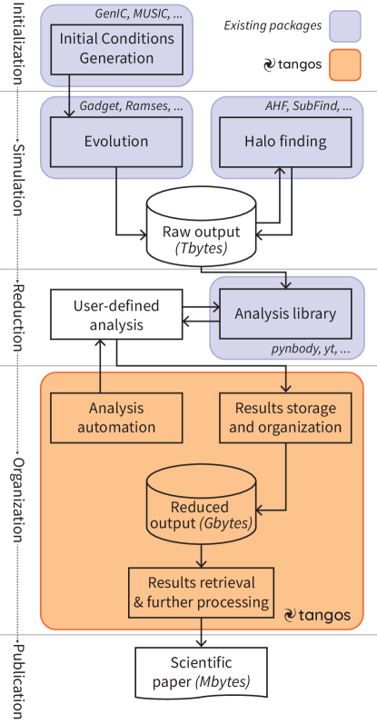
In the meantime, codes such as yt (Turk et al., 2011) and pynbody (Pontzen et al., 2013) have been maturing; these libraries present an abstracted view of raw simulation data, aiding the reduction layer but largely leaving organization to users. Both yt and pynbody contain some support for storing quantities such as profiles alongside halo catalogues, but not for managing the results of arbitrary user analysis. An add-on package for yt known as ytree can generate and traverse merger trees but the user must manually populate the data for each halo (unless using quantities already calculated and stored by the halo finder, which are unlikely to be sufficient for most use cases). Halotools (Hearin et al., 2017) is another existing code that addresses aspects of an organization layer: it includes sub-packages to turn halo catalogues into queryable merger trees. But its user tools are focussed on constructing semi-analytic models from these trees rather than populating them with properties calculated from the original simulation data.

Conversely, the kind of questions that tangos currently lends itself to answering center on hydrodynamic galaxy formation. How do star formation rates vary over time? What impact do mergers have on galaxy morphology? Where does a typical quasar line metal absorber lie relative to its nearest galaxy? Why does the distribution of dark matter get affected by some types of feedback but not others? By enabling many snapshots of multiple simulations to be linked together over time and efficiently queried, our ability to make progress in these areas has been enhanced.

Figure 2: An overview of the internal organization of tangos and its interaction with external libraries and users. By partitioning responsibilities between various sub-packages, tangos is made robust and flexible. Most modules are designed to be easily extensible. An overview is given in Section 2.

One way to conceive of a fully-fledged organization layer such as tangos is from the perspective of data compression. Raw output from the simulation layer can be extremely large (up to hundreds of terabytes) because it contains snapshots of the full dynamical state of the virtual universe at tens or hundreds of points in cosmological time. The goal of analysis is to move from the multi-terabyte raw output to a final, human-digestable set of information, nearly always in the form of one or more scientific publications. To put an upper limit on the information content of a paper, we can consider the literal file size of the associated PDF (perhaps a few megabytes). The compression ratio in moving from the raw output to the scientific results is therefore $10^{6}$ or more. Inserting the organization layer (giving two compression steps with ratios of order $10^{3}$) offers far greater clarity and flexibility than attempting to jump six orders of magnitude at once.

Some major simulation collaborations have made such intermediate data public. Structured Query Language (SQL) databases provided by the Millennium (Lemson & Virgo Consortium, 2006), MultiDark (Riebe et al., 2013), Eagle (McAlpine et al., 2016) and Theoretical Astronomical Observatory (Bernyk et al., 2016) groups provide good examples, as well as unstructured data releases with querying tools like those provided by the Illustris collaboration (Nelson et al., 2015). However these tools are specific to particular runs and pre-determined properties; they do not offer a mechanism for adding new information or generating databases from fresh simulations.

Tangos instead aims to minimize the human effort required to generate and collate complex results from new simulations of any type and scale. By providing a framework that is modularized, tangos is extensible in multiple directions. Adding new galaxy properties, querying techniques, parallelization methods, data storage approaches, file formats and analysis libraries are all possible (and in some cases, trivial). The code is freely available from github.com/pynbody/tangos under an open source (BSD 3-clause) license and compatible with Python 2.7 and 3.5 or later. The version of the code used to prepare this paper is 1.0.6 which is permanently available from Zenodo as Pontzen & Tremmel (2018), although we would always advise using the latest available version for new projects.

In this work we will discuss the overall structure of tangos and its modular components. Section 2 offers an overview of the full system, while sub-components are explored in Sections 3 to 10. We conclude in Section 11.

2 Overview

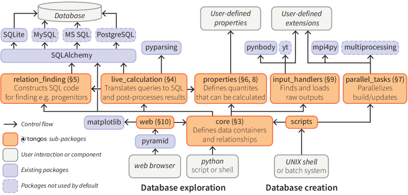
Tangos is implemented as a pure Python package and organized into multiple sub-packages. The relationship between the various sub-packages, user code and external dependencies is presented in Figure 2. Practical documentation for using tangos can be found at http://tiny.cc/tangos.

At its core our solution consists of a storage engine implemented atop SQLAlchemy which is a SQL toolkit and object relational mapper. SQLAlchemy does not constitute a database in its own right, but rather presents a unified high-level interface to multiple possible implementations such as SQLite, MySQL, MS-SQL and more. Our approach is described in Section 3 and implemented in the submodule core.

Querying the database can in principle be accomplished with raw SQL, but it is easier to use our exposed SQLAlchemy objects or higher-level functions. To aid constructing queries, especially those that traverse merger trees, we have implemented a domain-specific mini-language which is parsed using pyparsing and mapped into a combination of SQL and Python operations. This is implemented in the live_calculation module (Section 4). The construction of SQL queries for merger trees and other interrelationships between objects is delegated to the relation_finding module which is described in Section 5.

One of the strengths of the system is that users can easily define new galaxy properties to be calculated at each stored timestep. The framework allowing this extensibility is contained within the properties sub-package and described in Section 6. When calculating properties, tangos’ parallel_tasks sub-package enables parallelization via several strategies which are described in Section 7. We also allow rapidly time-varying quantities such as star formation rates to be stored and processed at a resolution finer than the snapshot steps, via a mechanism described in Section 8.

We factor out all tasks related to file loading and memory management to the input_handlers module which is covered by Section 9. By extending this module it is possible to work with any analysis toolkit for the reduction layer, although the default is pynbody.

The final component of tangos is its web server which enables databases to be explored from within a browser. The server, described in Section 10, does not implement any additional functionality; it simply provides an alternative interface that is convenient for rapid data exploration.

3 The core

Figure 3: The layout of the relational databases that tangos builds. Simulations can be associated with any number of timesteps which in turn can be associated with any number of objects (halos, black holes, or tracker regions). The objects have properties and links associated with them, forming the basic elements of a scientific analysis. While users do not have to be aware of this structure, we show it here because its layout is substantially different from that of existing databases (e.g. Lemson & Virgo Consortium, 2006; Riebe et al., 2013), reflecting the schemaless approach described in the text.

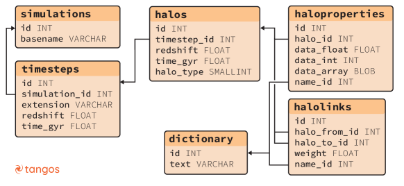
The core sub-package defines the layout of tangos databases; as we describe below this structure is not directly exposed to a typical user. Our databases are relational, consisting of a number of tables with pointers from one to another (Figure 3); our use of SQLAlchemy allows the user to choose from a wide variety of industry-standard underlying engines. By default we use SQLite which is a serverless system: the database consists of a single file, so that it can be downloaded from a cluster for offline analysis on a laptop or other device. A number of indexes are created alongside the tables, greatly enhancing the speed at which relevant queries may be executed at the cost of slightly increased storage space for the resulting database.

Each known simulation corresponds to a single entry in a simulations table, linking to multiple entries in a timesteps table, each of which in turn link to multiple entries in a halos table. It is worth noting that the halos table can, in fact, store multiple classes of object: halos, groups, tracked Lagrangian regions, or individual black holes. Each of these objects behaves similarly until the raw data is needed, at which point tangos automatically loads the appropriate portion. Because of the need to maintain backward compatibility during development, the table is still known as halos but we refer to a generic entry in the table as an object.

We associate any number of properties with each object. These might be quantities such as magnitudes and masses or arrays such as histograms and images. The properties are stored using a “schemaless” system, meaning that we do not create additional columns for each property but rather link to entries in a haloproperties table (with the name again reflecting a historical choice). Schemaless storage systems are popular in industrial applications (see e.g. MongoDB and schemaless). For tangos, the primary advantage is one of simplicity in managing the database: there is never any need to create or drop columns.

Our approach effectively attaches key-value pairs to each object; the keys are stored as a link to a separate dictionary table. Because querying is carried out through tangos itself (Section 4), the user need not be aware of any of these implementation details. Properties do not carry explicit units although this functionality is likely to be added in future.

In addition to storing properties, objects can also be linked to one another. Entries in a halolinks table describe this relationship between two objects; for example, one halo might be a progenitor, descendant, or subhalo of the other. We will discuss links and how they are used to generate informative science queries in Section 5, but first we consider the more elementary retrieval of properties from one or more objects.

4 Queries and calculations

The recommended approach to querying a tangos database is through the provided Python or web interfaces. Basic queries can be executed through a dictionary-like syntax. For example:

⬇

sim = tangos.get_simulation(’my_simulation’)

timestep = sim[42]

halo = timestep[5]

print(halo[’V_mag’])

will access the stored $V$ magnitude of halo $5$ in the $42$nd output of my_simulation. Each line of Python code is translated by tangos into a SQLAlchemy query, which in turn emits the correct dialect of SQL and returns the result.

This approach is acceptable for interactive exploration of small amounts of data. However when larger quantities of data are to be retrieved, issuing a series of multiple small queries is an inefficient approach since there is substantial latency associated with each round trip to the database. It is more time-effective to retrieve all required data in a single query. tangos offers multiple routes to optimizations of this sort.

For example, it is possible to retrieve properties from a series of objects, such as all those in a timestep. It is equally possible to retrieve multiple properties from each object. Combining both, the query

⬇

B, V = timestep.calculate_all("B_mag","V_mag")

returns two numpy arrays with respectively the B- and V-band magnitudes of every halo in the timestep. To achieve this, tangos generates and executes optimized SQL consisting of a double join from timesteps to halos and on to haloproperties.

We additionally implemented a mini-language to enable calculation within queries. The code

⬇

color = timestep.calculate_all("B_mag - V_mag")

results in the SQL join described above, but a post-processing step in Python takes the column difference before returning the resulting array to the user. While this simple example could be fully executed in SQL, the hybrid SQL–Python approach allows for more complex expressions. Users can even define functions which may be used within queries (see Section 6); a built-in example is the at function. The request

⬇

rho = timestep.\

calculate_all("at(Rvir/2, dm_density_profile)")

returns the value of the dark matter density profile evaluated at half the virial radius for each halo. Within calculate_all, the evaluation takes place in stages. First the user’s mini-language string is parsed and turned into an abstract syntax tree; by inspecting this tree, we can identify Rvir and dm_density_profile as the underlying properties to be retrieved. Next, the SQL is generated and emitted. Finally, the appropriate Python functions are called: a numpy-implemented divide operation followed by the interpolation function at which generates the final result.

The query system allows access to linked objects’ properties such as those from a halo’s major progenitor $n$ timesteps earlier. One might be interested in how much each galaxy’s magnitude has changed over the last $n=5$ steps, which corresponds to the query

⬇

dV = timestep.\

calculate_all("V_mag - earlier(5).V_mag")

Such calculations involve joins onto the requested properties from a heterogeneous set of halos which must first be identified using a merger tree. This is implemented within the relation_finding sub-package, as we now describe.

5 Merger trees and other relationships

Understanding how galaxies change over time is at the heart of many science analyses. This requires tangos to store and query merger trees, which express the hierarchical merging of structures (e.g. Kauffmann & White, 1993). We may additionally be interested in non-temporal relationships such as whether a particular halo is a subhalo of another, or to which halo a black hole is associated. As a final example, it can be useful to provide a map from halos in one simulation to those in another (given closely related simulations based on the same initial conditions). Tangos addresses all these needs by storing links between objects. Links are unidirectional and come with an associated weight which determines the strength of the relationship in a way to be defined shortly. The links are stored in an underlying table named halolinks. (As a reminder, the historically-chosen name belies that links do not have to connect halos: they can point from any object to any other.)

Each connection in a merger tree corresponds to two links pointing respectively forwards and backwards in time. This allows us to define independent weights for each direction by the number of particles in common as a fraction of the number in the link source. For a halo merging into a larger structure the forward weight will be close to $100\,\%$ whereas the reverse weight will give the merger ratio. The relation_finding sub-package is able to use this information to respond to queries as follows.

The sub-package assigns every halo a previous and next property such that the Python code

⬇

halo_prog = halo.previous

computes the major progenitor of halo in the previous timestep. When accessed by a user, previous generates and processes a suitable joined SQL query between the halos and halolink tables. If more than one linked halo is available, the link with the highest weight is selected (since other links point to smaller merging structures). The next property operates in a similar way.

While this is the simplest example of using links, there are considerably more powerful options available when multiple halos or timesteps are involved. We have implemented a series of strategies that efficiently find halos in several such scenarios. One typical use case is to collect properties along an entire major progenitor branch. To collate the color discussed in Section 4, we use the request

⬇

cols = halo.calculate_for_progenitors(’B_mag-V_mag’)

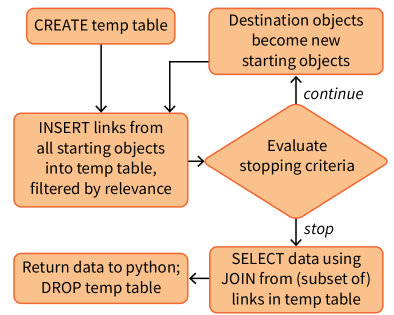
which will be executed in multiple stages within the database (Figure 4), followed by final processing in Python. The approach is to create a temporary table (which in most SQL implementations is possible without write access to the database) mirroring the structure of the halolinks table. It is first populated by inserting the links leading directly away from the initial objects. However only links satisfying a relevance criterion are included; for example, in the major progenitor search, they must point to an earlier timestep and have a weight higher than any other link to that timestep. Our implementation allows the filter to be redefined for different use cases (see below). The system next evaluates a stopping criterion against the links in the table; in the case of our progenitor search, it simply checks whether any new objects were uncovered in the most recent cycle. If so, the procedure starts again (now searching for links from the most recently discovered objects). If not, the recursion is complete.

By design, no data is transferred from SQL to Python during the recursion since this would be needlessly slow. Instead, at the end of the loop, the temporary table is handed to the live_calculation module. That system prepares a query against the temporary table joined to haloproperties as described in Section 4. The resulting columns are then retrieved and processed; the temporary table is dropped; and the results are returned.

The basic algorithm has been customized for a wide range of scenarios by subclassing the base MultiHopStrategy. In addition to the major progenitor search described so far, we have implemented subclasses that search for:

1. all progenitors (rather than major progenitors) – this required us to remove the highest-weight restriction in the definition of relevant links;

2. major descendants – accomplished by reversing the timestep comparison;

3. the major progenitor or descendant in a particular timestep (rather than all timesteps) – achieved by stopping once objects from that timestep are discovered, and selecting only those objects;

4. corresponding halos – defining relevant objects as those in another simulation at the same physical time, and stopping once such an object is discovered;

5. the most recent merger – similar to the all-progenitor search, but with a stopping criteria that halts when more than one progenitor is found in a single timestep.

Figure 4: The algorithm used to find relations such as major progenitors in a specified timestep. The database holds links only between adjacent timesteps, but by recursively populating a SQL temporary table, tangos can follow these links across multiple timesteps in an efficient way. User-requested data from the progenitors is acquired by a join onto the temporary table and delivered to Python at the end of the recursive process.

Users typically access these strategies through the live calculation mini-language. Consider the query given at the end of Section 4:

⬇

dV = timestep.\

calculate_all("V_mag - earlier(5).V_mag")

which requests, for each halo in timestep, the difference between the present $V$ magnitude and the major progenitor’s $V$ magnitude 5 timesteps earlier. For these purposes, strategy (iii) in the list above is applied. Use of other strategies is described in the documentation.

Taken together, the relation_finding and live_calculation modules allow tangos to execute queries that would be exceptionally hard to express within native SQL and prohibitively slow to implement in pure Python. Performance of the resulting system is explored in Figure 5 for a SQLite-backed database of a uniform volume simulation. Querying was undertaken on a 2013 Macbook Pro (Intel Core i7-4850HQ 2.3 GHz with 16GB RAM) running Python 3.6.1 and SQLite 3.13.0. We used a simulation with $100$ steps spaced equally in time between $z=1$ and $z=0$. This is unusually fine time spacing, but allows us to explore the performance implications of tracking large numbers of objects over many steps.

Figure 5: Performance for querying properties of the major progenitor of $N_{\mathrm{halo}}$ halos, $N_{\mathrm{step}}$ steps prior to a selected snapshot. Both panels show the same results, cutting across the 2D $(N_{\mathrm{halo}},N_{\mathrm{step}})$ plane in complementary ways. The time shown is the end-to-end tangos query runtime on a SQLite database for a uniform resolution simulation on a 2013 Macbook Pro (Intel Core i7-4850HQ 2.3 GHz with 16GB RAM). The runtimes are insensitive to the number of properties queried since the majority of time is spent in the relation_finding sub-package.

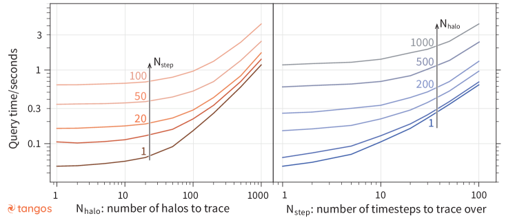
The panels of Figure 5 plot the same information projected along different axes. The two variables $N_{\mathrm{halo}}$ and $N_{\mathrm{step}}$ represent the number of halos to trace and of timesteps to jump. (We found that the number of properties ultimately retrieved from each halo is irrelevant since the time for computing progenitors is always the limiting factor.) As either $N_{\mathrm{step}}$ or $N_{\mathrm{halo}}$ becomes sufficiently large (exceeding $20$ or $100$ respectively) the scaling is approximately linear. The shallow scaling at smaller $N$ reflects the efficiency savings to be found in minimizing the number of SQL queries generated. Since the $N_{\mathrm{step}}=1$, $N_{\mathrm{halo}}=1$ case takes approximately $0.05$ seconds to complete, our most ambitious $N_{\mathrm{step}}=100$, $N_{\mathrm{halo}}=1000$ case would take well over an hour without optimization (compared to 4.2 seconds with the optimizations, over a thousand-fold improvement).

Bearing in mind that tangos sees the user’s time and patience as a limiting resource, this is a major enhancement. It enables more typical queries – say with $1000$ halos and $20$ timesteps – to complete in under two seconds. In this case, $320\,$ms is spent on building the temporary table which follows 1000 halos back through the merger tree; $1200\,$ms is spent filtering the completed temporary table and gathering the requested data; and $110\,$ms is spent on post-processing. The first two steps ($1520\,$ms) are carried out within the database engine, while the last ($110\,$ms) is executed by Python.

For some cosmological applications it may be useful to address a significantly larger number of halos; we can extrapolate the performance to query times of ten minutes for tracing $10^{6}$ halos over $20$ timesteps, although we did not explicitly test this. Improving run-times in this case would most likely be possible by replacing SQLite with a server-based database engine.

6 User-defined properties

Adapting tangos to a given science case requires the user to develop a set of properties which will be calculated for each object within the database. A new property is defined by implementing a subclass of PropertyCalculation. At a minimum, the property author must override names (which specifies one or more names of the properties to be stored) and calculate (which computes the values of those properties). The framework is responsible for passing raw data to calculate and for writing the returned value into the database. Therefore property classes express only scientific intent and do not take any responsibility for I/O.

Properties may either be dependent on existing entries in the database, or on the raw simulation snapshot data, or on both. For example, a halo virial velocity can be derived from an existing measurement of the virial mass but the calculation of a dark matter density profile would likely need access to the snapshot data. By default, any raw data provided to a calculation includes only the particles or cells within the object under consideration. However it is possible to provide a region_specification method to request access to a more extended volume; one use we have made of this facility is to measure inflows and outflows across the virial radius.

Tangos provides two routes to performing calculations: through a command-line script (tangos write) which writes results into the database, and through the live_calculation system which calculates on-the-fly during a query and does not store any output (Section 4). Properties requiring raw simulation data are only available when using the command-line tool. As we will discuss in the next section, the tangos write script can be parallelized at the halo or timestep level. Because the property class contains no explicit I/O, the implementer does not normally have to plan for different parallelization scenarios and can instead focus on science goals.

7 Parallelization strategies

Tangos offers a parallelization scheme, implemented by parallel_tasks, for use when building or updating databases. It is primarily targeted towards systems with a Message Passing Interface (MPI) library available, although it can also make use of Python’s multiprocessing module in place of MPI if necessary.

Given that analysis typically consumes a small fraction of the total computing resources of a simulation, our focus in implementing parallelization is on user convenience rather than machine efficiency. Nonetheless reduction of simulation data to a set of properties is a near-perfectly parallel process since each halo (or, potentially, timestep) can be considered independently of all others. This independence allows tangos to offer multiple parallelization options, each with differing benefits. Users select from these options at tangos write runtime by specifying a load mode.

In practice any given load mode is reliant on the input handler (Section 9) which is responsible for providing data as the parallel calculation proceeds. Here, we describe the parallel capabilities of the default pynbody input handler which implements four modes. The user starts tangos write through mpirun which launches multiple processes; all load modes use the first of these as a server with differing responsibilities as follows.

In the default load mode (which is applied if the user does not specify an alternate), the server assigns entire timesteps to all other processes. The cores then operate independently on each snapshot, running through the requested calculations for relevant halos and other objects. The chief advantage of this approach is simplicity and lack of communication overheads. However, it can lead to problematically large demands on memory: the number of cores used per node will need to be manually reduced using an appropriate invocation of mpirun if the size of a snapshot $M_{\mathrm{snap}}$ is too large (i.e. if $NM_{\mathrm{snap}}>M_{\mathrm{node}}$ where $M_{\mathrm{node}}$ is the total RAM available per node and $N$ is the number of MPI processes per node). Reducing $N$ may anyway be desirable if the property calculations are themselves parallelized using threads (see below).

When the partial load mode is specified, the server operates similarly but each individual core activates pynbody’s partial loading. This avoids the full simulation snapshot being retrieved from disk, instead loading the data for a single halo at a time. Partial loading is a simple solution to reducing memory usage, but can lead to excessive disk access (especially for network file systems) as multiple processes may simultaneously access data spread in near-random patterns across large files. It is also not advisable to load particle data from custom regions (Section 6) in this way, since currently such requests to pynbody can only be satisfied by scanning the properties of all particles in the snapshot.

The server load mode addresses these shortcomings by taking an entirely different approach. The server process takes responsibility for loading an entire snapshot, and then instructs the worker processes to perform calculations for individual halos or other objects. These cores respond with a request (or possibly multiple requests) for the raw data required. The chief advantage of this approach compared with partial loading is that disk access is consolidated into a larger, sequential read. The peak memory usage of server mode is only slightly greater than $M_{\mathrm{snap}}$, and this peak only occurs on the first node. In systems with heterogeneous hardware, it is possible to assign the server process to a machine with expanded RAM (e.g. the bigmem nodes on NASA’s Pleiades) while using regular nodes for the calculations. If the memory cost of loading an entire snapshot is still prohibitive, a hybrid server-partial mode loads only minimal information such as particle positions rather than the entire snapshot on the server. The individual worker nodes then load the relevant portions of all other arrays through the partial-loading approach.

One drawback of server mode is that it can generate significant MPI traffic to remote nodes which continually require new data. A final alternative, multi-server, is currently being planned where each node runs its own local server process. Provided every node has $M_{\mathrm{machine}}>M_{\mathrm{snap}}$ this approach should offer greater efficiency by minimizing network traffic.

In tandem with all the above, the user can implement their own per-halo shared-memory parallelization (based on threads or OpenMP from cython) and reduce the number of MPI processes spawned to free up physical processing cores. This approach to parallelization can be highly efficient but will typically require effort for the property implementer, unless the calculation is chiefly carried out by library routines. Luckily many pynbody built-in routines (such as smoothing and image rendering) are already parallelized with threads. The optimal balance of threads and MPI processes for a particular calculation can be determined empirically if required.

8 Sub-step time resolution

In Section 6, we discussed how new properties can be associated with objects at each timestep; their variation over time can then be inspected using the algorithms from Section 5. However, this ties the time resolution of stored properties to the simulation’s snapshot interval whereas many analyses of galaxy formation benefit from studying more rapid variations. The star formation or black hole accretion rates can vary by orders of magnitude over even a small fraction of a galaxy’s dynamical time. It is infeasible to store and process snapshots at sufficiently regular intervals to capture such short timescales.

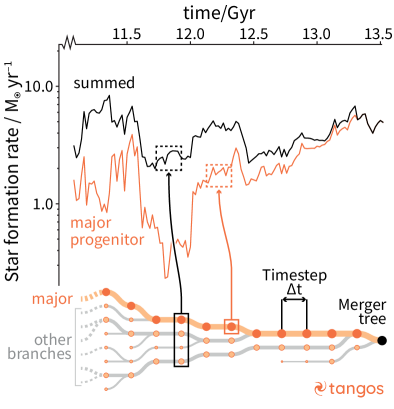
Simulation codes can work around this problem by storing auxiliary data such as formation times for each star particle or a black hole accretion log. Tangos incorporates a general mechanism to organize this information into time chunks, illustrated in Figure 6. In our scheme, the recent history of star formation or accretion is stored with each halo, black hole, or other object in each timestep. When the user attempts to access a time-chunked property, reassembly is automatically initiated: by default, tangos finds all major progenitors of the object and retrieves a chunk from each. It then constructs a history by gluing the chunks together (orange line, Figure 6). This approach allows significant flexibility in the manner of reassembly. For example, the user can request chunks to be summed over all progenitors (black line in Figure 6) rather than following the major progenitor branch.

From the property implementer’s perspective, using time chunking is straight-forward; instead of deriving from PropertyCalculation we derive from TimeChunkedPropertyCalculation which implements the reassembly discussed above. From a database user’s perspective, the mechanism is almost totally transparent because the reassembly process is triggered by any request for the property. Switching modes to obtain a summed history requires use of the mini-language function reassemble, which is further described in the user documentation.

9 File handling

Figure 6: The mechanism for storing and reconstructing time series with finer-than-timestep resolution, illustrated for a star formation rate history. Each halo stores a small chunk of history that covers the time back to the previous stored step. When the star formation rate is retrieved, tangos automatically reassembles the individual chunks into a complete high-resolution history. The user can control whether to include only the major progenitor branch or, conversely, sum over all branches.

We discussed in Section 6 how the tangos write tool loads data from a raw simulation and provides it to users’ property calculations. In addition, a load method is associated with each object; this allows raw data to be loaded into a standard Python session. Both approaches are implemented by the sub-package input_handlers which by default uses the pynbody library to load the underlying snapshot. We have been careful to isolate pynbody references to within a single class which is used only if required (specifically PynbodyInputHandler) so that the system can be fully decoupled; for example, an alternative YtInputHandler is provided to use the yt library in pynbody’s place. Users can straightforwardly re-implement this functionality using different libraries if required.

In addition to loading the raw data on demand, input handlers take responsibility for a diverse range of operations such as searching the file system for available snapshots and enumerating the halos and other objects within those snapshots. All these operations are therefore user-customizable. Handlers are implemented by deriving a class from HandlerBase and overriding a few methods to provide the required functionality. In particular, the data returned from an object’s load method and passed to PropertyCalculation instances is simply that returned from the underlying handler’s load_object method. A custom handler class can be specified when adding the simulation to a tangos database (through the tangos add script); it is then automatically used for all future operations requiring data from that particular simulation.

Adapting an existing input handler is also straight forward; one can derive from an existing class (such as PynbodyInputHandler) and override only those functions which need customization. The current version of tangos includes minor adaptations for working with different file formats; for example, when working with SubFind catalogues, it is helpful to make distinctions between groups and halos that do not necessarily exist with other halo finders. Further information can be found in the user documentation.

10 Web server

Figure 7: Two example pages from the web server. (Left) the timestep view, displaying one row per object and customizable columns which can be added, edited or removed and accept input in the live calculation mini-language for interactive queries. (Right) the halo view, which also contains a plots panel, here configured to show the halo merger tree. The rows are again editable, allowing for queries to be constructed and plotted from within a browser.

To enable rapid exploration of the database by users, collaborators and the broader community, tangos includes a web server built with the pyramid framework. Typically a user will launch the server application on their own machine and connect to localhost. As a safe default, our pyramid setup will not accept connections from external machines (although it can be tunnelled through SSH to a remote analysis node). If desired pyramid can be installed on a server and made world-accessible through a single change to the configuration file.

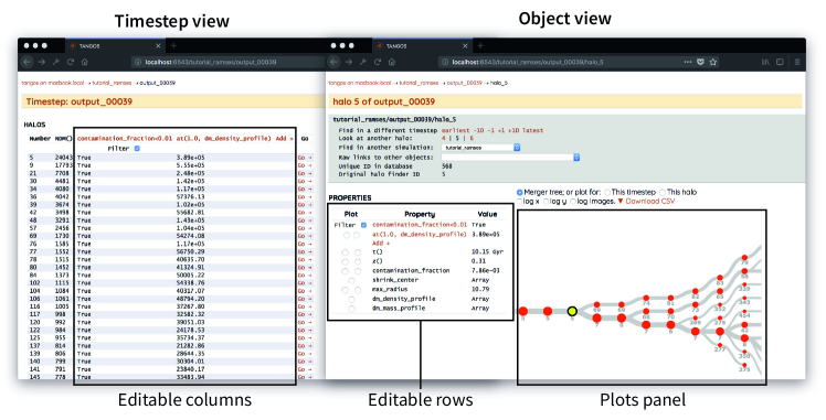
The pages served by tangos follow a natural hierarchy: the front page contains a list of known simulations, with links to subsequent pages listing timesteps and then objects. In Figure 7 we show the latter two stages using screenshots from a tutorial video. The left panel shows the timestep view. In addition to basic information about each halo the user may add any number of columns using the mini-language described in Section 4; as usual, this is parsed and executed by the live_calculation module. Here, for example, a query to determine whether the halo is in the high-resolution portion of a zoom simulation has been added, as well as a query which retrieves the dark matter density at $1.0\,\mathrm{kpc}$.

The right panel of Figure 7 shows the object view. It contains editable rows which correspond to the columns in the timestep view. Additionally it can be used to display a variety of plots; in this instance an interactive graphical representation of the merger tree has been generated. This is handled by the relation_finding sub-package, which uses the all-progenitor strategy (Section 5) to trace the tree (pruned by user-defined criteria such as minimum mass ratios).

Enabling interactivity requires part of the web module to be written in JavaScript and executed within the browser. When the user interacts with a page, the JavaScript code places asynchronous requests to Python over HTTP. The server calls the relevant functionality within tangos and encodes the results into JSON (JavaScript Object Notation); once the results arrive back in the browser, JavaScript places them into the appropriate elements within the page. Plots are generated using the matplotlib library and returned as a PNG file, with the exception of merger trees which are returned as JSON and rendered by the JavaScript library d3.

11 Conclusions

We have outlined the design of tangos, a system for generating and querying databases describing halos and other objects within cosmological simulations. We argued that the system forms a natural ‘organization layer’ within the simulation workflow (Figure 1). Sharpening this division of responsibilities has allowed us to carry out cleaner, more focussed and more reproducible science analyses.

Tangos aims, above all else, to present the simplest possible interface and so let users focus on physics. Computing efficiency is a secondary consideration. This differs from the simulation layer where the priority is typically to extract maximum performance from the hardware. There is a simple reason for this difference: the fraction of CPU resources spent on the reduction and organization layers is, in our experience, one to two orders of magnitude smaller than the cost of the simulation layer. On the other hand, the fraction of human time devoted to the analysis is by far the largest. Consequently tangos regards human attention as the most constrained resource.

An effective organization layer has a much broader range of responsibilities (Figure 1) than a static database. The modularity of tangos allows these diverse needs — ranging from analysis parallelization to data organization and query optimization — to be satisfied by near-independent sub-packages (Figure 2). Despite this separation, the sub-packages work together coherently, enabling a range of benefits:

• Queries are expressed in language that reflects scientific intent – but are also fast, as they are translated into carefully optimized joins executed by industry-standard database libraries (Sections 4 and 5). The resulting interface is sufficiently simple that we have been able to use it with undergraduate classes, allowing them to undertake projects quantifying the relative role of mergers and smooth accretion in building the halo population.

• We have been able to abstract away from halos to a broader class of objects in the database, including black holes and tracked Lagrangian regions. Especially in combination with the links system (Section 5), this allowed us to perform simultaneous analysis of the evolution of galaxies and their black holes (e.g. Tremmel et al., 2017; Di Cintio et al., 2017) as well as dynamical analyses of stellar subpopulations tracked over time (Pontzen et al., 2015).

• When building databases, users can implement analysis that is small, readable and devoid of any I/O. We have found this aspect particularly useful when combining analyses of multiple collaborators into final science results (e.g. Pontzen et al., 2017), a task that would previously involve wrangling multiple files in different formats.

• Parallelization of the database-building process is simple to apply (no analysis code needs to be changed; Section 7). This enabled us to scale from a package initially focussed on zoom simulations to one capable of ingesting state-of-the-art uniform volume runs (Tremmel et al., 2017).

• Queries can be executed from Python or from a web browser (Section 10). This opens up an agile mode of working where we perform rapid exploration of our data within a browser, before generating final versions of science plots using Python.

Tangos is an ongoing project and we hope that it will benefit from broader involvement. While the major development focus has been on enabling us to efficiently answer questions related to galaxy formation, the modular architecture should enable improvement and growth in multiple directions, coordinated by Github’s management tools and quality-assured by Travis automated testing. We are keen to discover whether the simulation community finds tangos helpful and we value all forms of feedback.

References

- Bernyk et al. (2016) Bernyk, M., Croton, D. J., Tonini, C., et al. 2016, ApJS, 223, 9
- Di Cintio et al. (2017) Di Cintio, A., Tremmel, M., Governato, F., et al. 2017, MNRAS, 469, 2845
- Hearin et al. (2017) Hearin, A. P., Campbell, D., Tollerud, E., et al. 2017, AJ, 154, 190
- Kauffmann & White (1993) Kauffmann, G., & White, S. D. M. 1993, MNRAS, 261, doi:10.1093/mnras/261.4.921
- Lemson & Virgo Consortium (2006) Lemson, G., & Virgo Consortium, t. 2006, ArXiv Astrophysics e-prints, astro-ph/0608019
- McAlpine et al. (2016) McAlpine, S., Helly, J. C., Schaller, M., et al. 2016, Astronomy and Computing, 15, 72
- Nelson et al. (2015) Nelson, D., Pillepich, A., Genel, S., et al. 2015, Astronomy and Computing, 13, 12
- Pontzen et al. (2015) Pontzen, A., Read, J. I., Teyssier, R., et al. 2015, MNRAS, 451, 1366
- Pontzen et al. (2013) Pontzen, A., Roškar, R., Stinson, G., & Woods, R. 2013, pynbody: N-Body/SPH analysis for python, Astrophysics Source Code Library, , , ascl:1305.002
- Pontzen & Tremmel (2018) Pontzen, A., & Tremmel, M. 2018, Zenodo, doi:10.5281/zenodo.1248829
- Pontzen et al. (2017) Pontzen, A., Tremmel, M., Roth, N., et al. 2017, MNRAS, 465, 547
- Pontzen et al. (2008) Pontzen, A., Governato, F., Pettini, M., et al. 2008, MNRAS, 390, 1349
- Riebe et al. (2013) Riebe, K., Partl, A. M., Enke, H., et al. 2013, Astronomische Nachrichten, 334, 691
- Tremmel et al. (2017) Tremmel, M., Karcher, M., Governato, F., et al. 2017, MNRAS, 470, 1121
- Turk et al. (2011) Turk, M. J., Smith, B. D., Oishi, J. S., et al. 2011, ApJS, 192, 9