Entanglement and diagonal entropies after a quench with no pair structure

Bruno Bertini Department of Physics, Faculty of Mathematics and Physics, University of Ljubljana, Jadranska 19, SI-1000 Ljubljana, Slovenia    Elena Tartaglia SISSA and INFN, via Bonomea 265, 34136, Trieste, Italy    Pasquale Calabrese SISSA and INFN, via Bonomea 265, 34136, Trieste, Italy International Centre for Theoretical Physics (ICTP), I-34151, Trieste, Italy
Abstract

A typical working condition in the study of quantum quenches is that the initial state produces a distribution of quasiparticle excitations with an opposite-momentum-pair structure. In this work we investigate the dynamical and stationary properties of the entanglement entropy after a quench from initial states which do not have such structure: instead of pairs of excitations they generate ν𝜈\nu-plets of correlated excitations with ν>2𝜈2\nu>2. Our study is carried out focusing on a system of non-interacting fermions on the lattice. We study the time evolution of the entanglement entropy showing that the standard semiclassical formula is not applicable. We propose a suitable generalisation which correctly describes the entanglement entropy evolution and perfectly matches numerical data. We finally consider the relation between the thermodynamic entropy of the stationary state and the diagonal entropy, showing that when there is no pair structure their ratio depends on the details of the initial state and lies generically between 1/2121/2 and 111.

I Introduction

Understanding how entanglement and correlations spread in out-of-equilibrium many-body quantum systems is an extremely fascinating topic which turned out to be of fundamental importance for several problems in condensed matter, statistical physics and quantum field theory. In this manuscript we focus on global quenches, in which an isolated many-body quantum system is prepared at t=0𝑡0t=0 in a finite-energy-density pure state |ψ0ketsubscript𝜓0|\psi_{0}\rangle, and for t>0𝑡0t>0 it is evolved unitarily with dynamics governed by a Hamiltonian H𝐻H (see the reviews pssv-11 ; gogolin-2015 ; vidmar-2016 ; calabrese-2016 ; cc-16 ; ef-16 ; quasilocal-16 ). The theoretical study of quench problems has been boosted by seminal cold-atom experiments langen-rev ; kinoshita-2006 ; hofferberth-2007 ; trotzky-2012 ; gring-2012 ; cheneau-2012 ; langen-2013 ; fukuhara-2013 ; langen-2015 ; bsjs-18 probing many different aspects of the non-equilibrium unitary dynamics of quantum systems.

If a many-body quantum system is in a pure state |ψket𝜓|\psi\rangle, the bipartite entanglement between a subsystem A𝐴A and its complement A¯¯𝐴\bar{A} may be measured by the entanglement entropy faziorev ; CCrev ; Eisrev ; Lafrev . This is defined as the von Neumann entropy of the reduced density matrix 𝝆ATrA¯|ψψ|subscript𝝆𝐴subscriptTr¯𝐴ket𝜓bra𝜓\boldsymbol{\rho}_{A}\equiv{\rm Tr}_{\bar{A}}|\psi\rangle\langle\psi| of the subsystem A𝐴A, i.e.

SATr𝝆Aln𝝆A.subscript𝑆𝐴Trsubscript𝝆𝐴subscript𝝆𝐴S_{A}\equiv-{\rm Tr}\boldsymbol{\rho}_{A}\ln\boldsymbol{\rho}_{A}. (1)

The time evolution of the entanglement entropy after a quantum quench has been the focus of intense research calabrese_evolution_2005 ; FC:XY ; alba_entanglement_2016 ; dsvc17 ; ep-08 ; nr-14 ; kormos-2014 ; leda-2014 ; collura-2014 ; bhy-17 ; hbmr-17 ; dmcf-06 ; lauchli-2008 ; hk-13 ; fc-15 ; buyskikh-2016 ; kctc-17 ; coser-2014 ; cotler-2016 ; nahum-17 ; p-18 ; fnr-17 ; r-2017 ; daley-2012 ; mkz-17 ; evdcz-18 ; ckt-18 ; CC:lq ; SD:lq ; PE:ql ; PE:ql2 ; mariolq ; brunolq ; ryulq ; alba-inh ; mbpc-17 ; BFPC18 . One of the main reasons for this fervent activity is technological: the rate of growth of the entanglement entropy determines whether it is feasible to simulate non-equilibrium quantum systems with tensor network algorithms swvc-08 ; swvc-08b ; pv-08 ; rev1 ; d-17 . Another reason was in relation to the key question on the emergence of thermodynamics from the microscopic quantum dynamics. There is now solid evidence indicating that the thermodynamic entropy in the local stationary state following the quench is nothing but the asymptotic entanglement entropy of a large subsystem calabrese_evolution_2005 ; alba_entanglement_2016 ; dls-13 ; bam-15 ; Gur14 ; SPR11 ; this is also supported by direct experimental evidence kaufman-2016 .

Despite years of intensive investigation, analytic ab-initio results for the entanglement entropy are scarce even for free theories because of the intrinsic difficulties in evaluating Eq. (1). Surprisingly, many qualitative features of the entanglement entropy evolution may be understood using a very simple physical picture proposed in Ref. calabrese_evolution_2005 . In this quasiparticle picture, the initial state produces pairs of excitations with opposite momentum. For t>0𝑡0t>0, the excitations with momentum k𝑘k move ballistically with group velocity v(k)𝑣𝑘v(k). The spreading of entanglement calabrese_evolution_2005 and correlations cc-06 ; cc-07 is interpreted in terms of entangled particles emitted from the same point in space. As the quasiparticles move far apart, larger regions of the system get entangled: at a given time, the entanglement entropy of the subsystem A𝐴A is due to those quasiparticles that, emitted from the same point in space, are shared between subsystem A𝐴A and its complement. Thus, for an interval A𝐴A of length \ell embedded in an infinite one-dimensional system we have calabrese_evolution_2005

SA(t)=2t2|v(k)|t<dk|v(k)|s(k)+2|v(k)|t>dks(k),subscript𝑆𝐴𝑡2𝑡subscript2𝑣𝑘𝑡differential-d𝑘𝑣𝑘𝑠𝑘subscriptconditional2𝑣𝑘ket𝑡differential-d𝑘𝑠𝑘S_{A}(t)=2t\!\!\!\!\int\limits_{\!2|v(k)|t<\ell}\!\!\!\!{\rm d}k\,|v(k)|s(k)+\ell\!\!\!\!\int\limits_{2|v(k)|t>\ell}\!\!\!\!{\rm d}k\,s(k)\,, (2)

where we weighted the quasiparticles with a factor s(k)𝑠𝑘s(k) which encodes the production rate of quasiparticles with momentum ±kplus-or-minus𝑘\pm k and their individual contribution to the entanglement entropy.

Obviously this picture is strictly valid only for those models where all quasiparticles have an infinite lifetime, i.e. in integrable models. It gives, however, important qualitative and quantitative information in many other circumstances as well, see, e.g., Refs. kctc-17 ; ckt-18 . For integrable models, Eq. (2) is expected to be asymptotically exact in the space-time scaling limit t,𝑡t,\ell\to\infty with the ratio t/𝑡t/\ell fixed. When a maximum quasiparticle velocity vM|v(k)|subscript𝑣𝑀𝑣𝑘v_{M}\geq|v(k)| exists (e.g., as a consequence of the Lieb-Robinson bound lieb-1972 ), Eq. (2) predicts that for t/(2vM)𝑡2subscript𝑣𝑀t\leq\ell/(2v_{M}), the entanglement entropy grows linearly in time because the second term in (2) vanishes. Conversely, for t/(2vM)much-greater-than𝑡2subscript𝑣𝑀t\gg\ell/(2v_{M}), only the second term is nonzero and SA(t)subscript𝑆𝐴𝑡S_{A}(t) becomes extensive in the subsystem size, namely SA(t)proportional-tosubscript𝑆𝐴𝑡S_{A}(t)\propto\ell.

In order to turn (2) into a quantitative prediction, one should be able to determine the two functions s(k)𝑠𝑘s(k) and v(k)𝑣𝑘v(k). In particular, v(k)𝑣𝑘v(k) is naturally identified with the velocity of excitations over the stationary state alba_entanglement_2016 , which can be readily computed by Bethe ansatz BEL:prl . Computing s(k)𝑠𝑘s(k) from first principles is, however, a formidable task even for free models (see e.g. FC:XY ). A key observation of Ref. alba_entanglement_2016 was that such an ab-initio calculation is not necessary: one can conjecture the form of the function s(k)𝑠𝑘s(k) by imposing the equality between the entanglement and the thermodynamic entropy in the stationary state. One notes that for integrable models the stationary state is given by a generalised Gibbs ensemble (GGE), which takes into account all the constraints imposed by the local and quasi-local integrals of motion vidmar-2016 ; ef-16 ; quasilocal-16 ; rigolGGE . The determination of the thermodynamic entropy in the GGE is a standard equilibrium calculation and the entropy density in momentum space s(k)𝑠𝑘s(k) can be easily read off. The resulting s(k)𝑠𝑘s(k) is finally used as entry in the quasiparticle formula (2) making it quantitative. Importantly, this prediction is obtained without solving the complex many-body dynamics.

A crucial assumption behind the conjecture (2) is that the initial state acts as a source of pairs of quasiparticle excitations with opposite momentum. In Bethe-ansatz language this assumption may be viewed as a consequence of the requirement that only parity-invariant eigenstates (as defined in dwbc-14 ; cd-12 ) have nonzero overlap with the initial state. It has been recently shown (first for quantum field theories delfino-14 ; schuricht_quantum_2015 and then for lattice integrable models PPV:integrablestateslattice ) that only quenches originating from these initial states are compatible with some integrability requirements that strongly simplify the solution of the quench problem. Indeed, so far, all the overlaps which are exactly known in interacting integrable models on the lattice, satisfy the parity invariant constraint dwbc-14 ; cd-12 ; pc-14 ; pozsgay-14 ; bdwc-14 ; cd-14 ; fz-16 ; dkm-16 . Moreover, states with this structure give a good approximation of the initial state after mass and interaction quenches in the sinh-Gordon field theory sotiriadis_zamolodchikov_2012 ; sotiriadis_boundary_2014 ; horvath_initial_2016 ; horvath_overlaps_2017 . States with nonzero overlap with generic eigenstates or with different families of eigenstates do, however, exist, and it is of fundamental importance to understand if and how (2) could generalise. A very useful playground where one can gain valuable insight into this question is represented by free models, since there quench problems can be readily solved even for initial states with a more general overlap structure.

In a recent paper previousepisode , in the context of quantum quenches for Hubbard model with infinite repulsion, we constructed several families of initial states that have nonzero overlap with states formed by generic multiplets of quasiparticles and not only pairs. Analogous states can be constructed for free spinless fermions hopping on a one-dimensional line, and the time evolution from such states can be determined exactly. This is precisely the goal of this paper: we study the dynamics of free fermions after quenches from states with no pair structure, focusing on the dynamics of entanglement entropy and its relation with the diagonal entropy. We work out a suitable generalisation of (2) which shows a highly nontrivial structure: for example, we show that its form cannot be fixed solely by requiring that the stationary value of the entanglement entropy and the thermodynamic entropy be equal. Moreover, we show that the stationary value of the entanglement entropy is generically not related to the diagonal entropy. Although we focus on the von Neumann entropy (1), our findings apply to all Rényi entanglement entropies as for free systems the complications encountered in defining them ac-17b ; ac-17c are not present.

The manuscript is organised as follows. In Sections II and III we respectively present the model and the family of initial states considered, while in Section IV we determine the stationary state describing expectation values of local observables at infinite times after the quench. In Section V we analyse the time evolution of the entanglement entropy, and in Section VI we study the relation between the stationary value of the entanglement entropy and the diagonal entropy. Finally, in Section VII we report our conclusions. Three appendices complement the main text with a number of technical points.

II Model

We consider spinless fermions on the lattice, whose dynamics are described by the following Hamiltonian

H^=Jx=1L(cxcx1+cx1cx)c0=cL.formulae-sequence^𝐻𝐽superscriptsubscript𝑥1𝐿superscriptsubscript𝑐𝑥subscriptsuperscript𝑐absent𝑥1superscriptsubscript𝑐𝑥1subscriptsuperscript𝑐absent𝑥subscript𝑐0subscript𝑐𝐿\hat{H}=-J\sum_{x=1}^{L}\left(c_{x}^{\dagger}c^{\phantom{\dagger}}_{x-1}+c_{x-1}^{\dagger}c^{\phantom{\dagger}}_{x}\right)\qquad\qquad c_{0}=c_{L}\,. (3)

Here the fermionic operators cxsubscript𝑐𝑥c_{x} and cxsuperscriptsubscript𝑐𝑥c_{x}^{\dagger} satisfy the canonical anti-commutation relations

{cx,cy}={cx,cy}=0,{cx,cy}=δx,y.formulae-sequencesubscript𝑐𝑥subscript𝑐𝑦superscriptsubscript𝑐𝑥superscriptsubscript𝑐𝑦0subscript𝑐𝑥superscriptsubscript𝑐𝑦subscript𝛿𝑥𝑦\{c_{x},c_{y}\}=\{c_{x}^{\dagger},c_{y}^{\dagger}\}=0,\qquad\qquad\{c_{x},c_{y}^{\dagger}\}=\delta_{x,y}\,. (4)

We also introduce the unitary translation T^^𝑇\hat{T} and reflection R^^𝑅\hat{R} operators acting as follows on the fermionic operators

T^cxT^=cx+1,R^cxR^=cL+1x.formulae-sequence^𝑇subscriptsuperscript𝑐𝑥superscript^𝑇subscriptsuperscript𝑐𝑥1^𝑅subscriptsuperscript𝑐𝑥superscript^𝑅subscriptsuperscript𝑐𝐿1𝑥\hat{T}c^{\dagger}_{x}\hat{T}^{\dagger}=c^{\dagger}_{x+1}\,,\qquad\qquad\qquad\hat{R}c^{\dagger}_{x}\hat{R}^{\dagger}=c^{\dagger}_{L+1-x}\,. (5)

The Hamiltonian (3) is readily diagonalised by Fourier transform

c~k=1Lx=1Leikxcx,k=2πLn,n[L2,L2),formulae-sequencesubscript~𝑐𝑘1𝐿superscriptsubscript𝑥1𝐿superscript𝑒𝑖𝑘𝑥subscript𝑐𝑥formulae-sequence𝑘2𝜋𝐿𝑛𝑛𝐿2𝐿2\tilde{c}_{k}=\frac{1}{\sqrt{L}}\sum_{x=1}^{L}e^{ikx}c_{x}\,,\qquad\qquad k=\frac{2\pi}{L}n\,,\qquad\qquad n\in\mathbb{Z}\cap[-\tfrac{L}{2},\tfrac{L}{2})\,, (6)

this transformation preserves the commutation relations

{c~k,c~p}={c~k,c~p}=0,{c~k,c~p}=δk,p.formulae-sequencesubscript~𝑐𝑘subscript~𝑐𝑝superscriptsubscript~𝑐𝑘superscriptsubscript~𝑐𝑝0subscript~𝑐𝑘superscriptsubscript~𝑐𝑝subscript𝛿𝑘𝑝\{\tilde{c}_{k},\tilde{c}_{p}\}=\{\tilde{c}_{k}^{\dagger},\tilde{c}_{p}^{\dagger}\}=0,\qquad\qquad\{\tilde{c}_{k},\tilde{c}_{p}^{\dagger}\}=\delta_{k,p}\,. (7)

After the transformation the Hamiltonian reads as

H^=kε(k)c~kc~k,ε(k)2Jcos(k).formulae-sequence^𝐻subscript𝑘𝜀𝑘subscriptsuperscript~𝑐𝑘subscriptsuperscript~𝑐absent𝑘𝜀𝑘2𝐽𝑘\hat{H}=\sum_{k}\varepsilon(k)\tilde{c}^{\dagger}_{k}\tilde{c}^{\phantom{{\dagger}}}_{k}\,,\qquad\qquad\qquad\varepsilon(k)\equiv-2J\cos(k)\,. (8)

Since

eiH^tc~keiH^t=c~keiε(k)t,T^c~kT^=c~keik,formulae-sequencesuperscript𝑒𝑖^𝐻𝑡subscriptsuperscript~𝑐𝑘superscript𝑒𝑖^𝐻𝑡subscriptsuperscript~𝑐𝑘superscript𝑒𝑖𝜀𝑘𝑡^𝑇subscriptsuperscript~𝑐𝑘superscript^𝑇subscriptsuperscript~𝑐𝑘superscript𝑒𝑖𝑘e^{i\hat{H}t}\tilde{c}^{\dagger}_{k}e^{-i\hat{H}t}=\tilde{c}^{\dagger}_{k}e^{i\varepsilon(k)t}\,,\qquad\qquad\hat{T}\tilde{c}^{\dagger}_{k}\hat{T}^{\dagger}=\tilde{c}^{\dagger}_{k}e^{ik}\,, (9)

the operators c~k(c~k)subscriptsuperscript~𝑐𝑘subscriptsuperscript~𝑐absent𝑘\tilde{c}^{{{\dagger}}}_{k}\,(\tilde{c}^{\phantom{{\dagger}}}_{k}) are interpreted as those creating (destroying) a quasiparticle of momentum k𝑘k and energy ε(k)𝜀𝑘\varepsilon(k). A basis of eigenstates of (3) is naturally given by the “scattering states” of such quasiparticles

𝒮={|ΨN(k1,,kN)c~k1c~kN|0:N,ki=2πLni,ni[L2,L2),ni<ni+1,i},\mathcal{S}=\{\ket{\Psi_{N}(k_{1},\ldots,k_{N})}\equiv\tilde{c}^{\dagger}_{k_{1}}\ldots\tilde{c}^{\dagger}_{k_{N}}\ket{0}:\quad N\in\mathbb{N},\quad k_{i}=\frac{2\pi}{L}n_{i},\quad n_{i}\in\mathbb{Z}\cap[-\tfrac{L}{2},\tfrac{L}{2}),\quad n_{i}<n_{i+1},\ \forall i\}\,, (10)

where |0ket0\ket{0} is the “vacuum state” such that

c~k|0=0k.subscript~𝑐𝑘ket00for-all𝑘\tilde{c}_{k}\ket{0}=0\qquad\forall k\,. (11)

The state |ΨN(k1,,kN)ketsubscriptΨ𝑁subscript𝑘1subscript𝑘𝑁\ket{\Psi_{N}(k_{1},\ldots,k_{N})} has energy and momentum given by

E(k1kN)=i=1Nε(ki),P(k1kN)=[i=1Nki]mod 2π.formulae-sequence𝐸subscript𝑘1subscript𝑘𝑁superscriptsubscript𝑖1𝑁𝜀subscript𝑘𝑖𝑃subscript𝑘1subscript𝑘𝑁delimited-[]superscriptsubscript𝑖1𝑁subscript𝑘𝑖mod2𝜋E(k_{1}\ldots k_{N})=\sum_{i=1}^{N}\varepsilon(k_{i})\,,\qquad\qquad P(k_{1}\ldots k_{N})=\left[\sum_{i=1}^{N}k_{i}\right]\text{mod}\,2\pi\,. (12)

In the thermodynamic limit, limthsubscriptth\lim_{\rm th}, when one sends the volume of the system to infinity keeping the particle density fixed, the momenta kisubscript𝑘𝑖k_{i} become continuous variables and the eigenstates are conveniently parametrised by their density

ρ(ki)=limth1L(kiki+1),𝜌subscript𝑘𝑖subscriptth1𝐿subscript𝑘𝑖subscript𝑘𝑖1\rho(k_{i})={\textstyle\lim_{\rm th}}\frac{1}{L(k_{i}-k_{i+1})}\,, (13)

called the root density.

III Initial states

Our goal in this paper is to study the time evolution generated by the Hamiltonian (3) on the following class of states

|Φ{a0,,aν1}νketsubscriptsuperscriptΦ𝜈subscript𝑎0subscript𝑎𝜈1\displaystyle\ket{\Phi^{\nu}_{\{a_{0},\ldots,a_{\nu-1}\}}} =j=1L/ν(m=0ν1amcνjm)|0,j=0ν1|aj|2=1,formulae-sequenceabsentsuperscriptsubscriptproduct𝑗1𝐿𝜈superscriptsubscript𝑚0𝜈1subscript𝑎𝑚subscriptsuperscript𝑐𝜈𝑗𝑚ket0superscriptsubscript𝑗0𝜈1superscriptsubscript𝑎𝑗21\displaystyle=\prod_{j=1}^{L/\nu}\left(\sum_{m=0}^{\nu-1}a_{m}c^{\dagger}_{\nu j-m}\right)\ket{0}\,,\qquad\qquad\sum_{j=0}^{\nu-1}|a_{j}|^{2}=1\,, (14)

well-defined in finite volume L𝐿L such that L/ν𝐿𝜈L/\nu is integer. These states are invariant under translation of ν𝜈\nu sites (up to a global phase) and are Gaussian, i.e. Wick’s theorem holds on these states. The latter property follows by observing that they can be written as vacuum states for an appropriately defined set of fermionic operators, related to cx,cxsubscript𝑐𝑥superscriptsubscript𝑐𝑥c_{x},c_{x}^{\dagger} by a linear transformation molinari_notes_2017 . Such a set of fermionic operators is explicitly constructed in Appendix A.

Before describing further properties of these states, we report some simple examples to clarify their structure. Taking ν=3𝜈3\nu=3 and denoting fermions with a closed circle and empty sites with an open circle, we begin with two examples where only one aisubscript𝑎𝑖a_{i} is nonzero

|Φ{1,0,0}3ketsubscriptsuperscriptΦ3100\displaystyle\ket{\Phi^{3}_{\{1,0,0\}}} =j=1L/3c3j|0=|🌕🌕🌑🌕🌕🌑🌕🌕🌑absentsuperscriptsubscriptproduct𝑗1𝐿3subscriptsuperscript𝑐3𝑗ket0ket🌕🌕🌑🌕🌕🌑🌕🌕🌑\displaystyle=\prod_{j=1}^{L/3}c^{\dagger}_{3j}\ket{0}=\ket{\fullmoon\fullmoon\newmoon\,\fullmoon\fullmoon\newmoon\,\fullmoon\fullmoon\newmoon\ldots} (15)
|Φ{0,1,0}3ketsubscriptsuperscriptΦ3010\displaystyle\ket{\Phi^{3}_{\{0,1,0\}}} =j=1L/3c3j1|0=|🌕🌑🌕🌕🌑🌕🌕🌑🌕absentsuperscriptsubscriptproduct𝑗1𝐿3subscriptsuperscript𝑐3𝑗1ket0ket🌕🌑🌕🌕🌑🌕🌕🌑🌕\displaystyle=\prod_{j=1}^{L/3}c^{\dagger}_{3j-1}\ket{0}=\ket{\fullmoon\newmoon\fullmoon\,\fullmoon\newmoon\fullmoon\,\fullmoon\newmoon\fullmoon\ldots} (16)

In these cases, the state is comprised of repeated blocks of ν=3𝜈3\nu=3 sites. Instead, if we take both a0=a1=1/2subscript𝑎0subscript𝑎112a_{0}=a_{1}=1/\sqrt{2}, we obtain a sum of terms where each block of three either has a fermion in the last or the middle position

|Φ{1/2,1/2,0}3ketsubscriptsuperscriptΦ312120\displaystyle\ket{\Phi^{3}_{\{1/\sqrt{2},1/\sqrt{2},0\}}} =12L/6j=1L/3(c3j+c3j1)|0absent1superscript2𝐿6superscriptsubscriptproduct𝑗1𝐿3subscriptsuperscript𝑐3𝑗subscriptsuperscript𝑐3𝑗1ket0\displaystyle=\frac{1}{2^{L/6}}\prod_{j=1}^{L/3}(c^{\dagger}_{3j}+c^{\dagger}_{3j-1})\ket{0}
=12L/6[|🌕🌕🌑🌕🌕🌑🌕🌕🌑\displaystyle=\frac{1}{2^{L/6}}\left[\ket{\fullmoon\fullmoon\newmoon\,\fullmoon\fullmoon\newmoon\,\fullmoon\fullmoon\newmoon\ldots}\right.
+|🌕🌑🌕🌕🌕🌑🌕🌕🌑+|🌕🌕🌑🌕🌑🌕🌕🌕🌑+|🌕🌕🌑🌕🌕🌑🌕🌑🌕+ket🌕🌑🌕🌕🌕🌑🌕🌕🌑ket🌕🌕🌑🌕🌑🌕🌕🌕🌑ket🌕🌕🌑🌕🌕🌑🌕🌑🌕\displaystyle+\ket{\fullmoon\newmoon\fullmoon\,\fullmoon\fullmoon\newmoon\,\fullmoon\fullmoon\newmoon\ldots}+\ket{\fullmoon\fullmoon\newmoon\,\fullmoon\newmoon\fullmoon\,\fullmoon\fullmoon\newmoon\ldots}+\ket{\fullmoon\fullmoon\newmoon\,\fullmoon\fullmoon\newmoon\,\fullmoon\newmoon\fullmoon\ldots}+\ldots
+|🌕🌑🌕🌕🌑🌕🌕🌕🌑++|🌕🌑🌕🌕🌑🌕🌕🌑🌕].\displaystyle+\left.\ket{\fullmoon\newmoon\fullmoon\,\fullmoon\newmoon\fullmoon\,\fullmoon\fullmoon\newmoon\ldots}+\ldots+\ket{\fullmoon\newmoon\fullmoon\,\fullmoon\newmoon\fullmoon\,\fullmoon\newmoon\fullmoon\ldots}\right]\,. (17)

Note that these states are generically not reflection symmetric. Specifically, we have

R^|Φ{a0,,aν1}ν=(1)L2ν[Lν1]|Φ{aν1,,a0}ν.^𝑅ketsubscriptsuperscriptΦ𝜈subscript𝑎0subscript𝑎𝜈1superscript1𝐿2𝜈delimited-[]𝐿𝜈1ketsubscriptsuperscriptΦ𝜈subscript𝑎𝜈1subscript𝑎0\hat{R}\ket{\Phi^{\nu}_{\{a_{0},\ldots,a_{\nu-1}\}}}=(-1)^{\frac{L}{2\nu}\left[\frac{L}{\nu}-1\right]}\ket{\Phi^{\nu}_{\left\{a_{\nu-1},\ldots,a_{0}\right\}}}. (18)

The overlaps between the initial states (14) and the eigenstates (10) read as

Φ{am}ν|ΨN(𝒌)=inner-productsubscriptsuperscriptΦ𝜈subscript𝑎𝑚subscriptΨ𝑁𝒌absent\displaystyle\braket{\Phi^{\nu}_{\{a_{m}\}}}{\Psi_{N}(\boldsymbol{k})}= δN,L/νLN/2j=1N[=0ν1aeikj]detN{eiνkab}a,b=1,N.subscript𝛿𝑁𝐿𝜈superscript𝐿𝑁2superscriptsubscriptproduct𝑗1𝑁delimited-[]superscriptsubscript0𝜈1subscript𝑎superscript𝑒𝑖subscript𝑘𝑗subscript𝑁subscriptsuperscript𝑒𝑖𝜈subscript𝑘𝑎𝑏formulae-sequence𝑎𝑏1𝑁\displaystyle\frac{\delta_{N,{L}/\nu}}{L^{N/2}}\prod_{j=1}^{N}\!\left[{\sum_{\ell=0}^{\nu-1}a_{\ell}e^{-i\ell k_{j}}}\right]{\det}_{N}\{e^{i\nu k_{a}b}\}_{a,b=1\ldots,N}\,. (19)

These overlaps impose a macroscopic number of constraints on the eigenstates contributing to the dynamics, specifically we must have

N=Lν,kikj0mod2πνi,j=1,,Lν.formulae-sequence𝑁𝐿𝜈formulae-sequencesubscript𝑘𝑖subscript𝑘𝑗modulo02𝜋𝜈for-all𝑖𝑗1𝐿𝜈N=\frac{L}{\nu}\,,\qquad{k}_{i}-k_{j}\neq 0\!\!\!\mod\frac{2\pi}{\nu}\qquad\forall\,i,j=1,\dots,\frac{L}{\nu}\,. (20)

In words the second constraint means that for any given k2πL([ν22νL,12L))𝑘2𝜋𝐿𝜈22𝜈𝐿12𝐿k\in\frac{2\pi}{L}\left(\mathbb{Z}\cap[\tfrac{\nu-2}{2\nu}L,\tfrac{1}{2}L)\right) only one momentum in the set

{k,k2πνk2π(ν1)ν}𝑘𝑘2𝜋𝜈𝑘2𝜋𝜈1𝜈\left\{k,k-\frac{2\pi}{\nu}\,\ldots k-\frac{2\pi(\nu-1)}{\nu}\right\} (21)

can be occupied. Such constraint for ν=2𝜈2\nu=2 produces a pair structure in the eigenstates contributing to the time evolution: for each particle with momentum k2πL([ν22νL,12L))𝑘2𝜋𝐿𝜈22𝜈𝐿12𝐿k\in\frac{2\pi}{L}\left(\mathbb{Z}\cap[\tfrac{\nu-2}{2\nu}L,\tfrac{1}{2}L)\right) there is a hole with momentum kπ𝑘𝜋k-\pi and vice versa. For ν>2𝜈2\nu>2 the eigenstates have no pair structure: there are correlated ν𝜈\nu-plets formed by ν1𝜈1\nu-1 holes and one particle. Note that, for ν>2𝜈2\nu>2, such states are non-integrable according to the definition of Ref. PPV:integrablestateslattice .

IV The post-quench stationary state

By studying time evolution from the states |Φ{am}νketsubscriptsuperscriptΦ𝜈subscript𝑎𝑚\ket{\Phi^{\nu}_{\{a_{m}\}}}, it is easy to verify that one-site translational invariance is restored at infinite times; a proof of this statement is reported in Appendix B. As a consequence, the post-quench steady state is fully characterised by the mode occupations, i.e. the expectation values of the conserved operators ckcksubscriptsuperscript𝑐𝑘subscriptsuperscript𝑐absent𝑘c^{\dagger}_{k}c^{\phantom{{\dagger}}}_{k} on the initial state (14). An explicit calculation gives

Φ{am}ν|c~kc~k|Φ{am}νquantum-operator-productsubscriptsuperscriptΦ𝜈subscript𝑎𝑚subscriptsuperscript~𝑐𝑘subscriptsuperscript~𝑐absent𝑘subscriptsuperscriptΦ𝜈subscript𝑎𝑚\displaystyle\braket{\Phi^{\nu}_{\{a_{m}\}}}{\tilde{c}^{\dagger}_{k}\tilde{c}^{\phantom{{\dagger}}}_{k}}{\Phi^{\nu}_{\{a_{m}\}}} =1Ln,m=1Leik(mn)Φ{am}ν|cncm|Φ{am}ν=1νn,m=1νeik(mn)Φ{am}ν|cncm|Φ{am}νabsent1𝐿superscriptsubscript𝑛𝑚1𝐿superscript𝑒𝑖𝑘𝑚𝑛quantum-operator-productsubscriptsuperscriptΦ𝜈subscript𝑎𝑚subscriptsuperscript𝑐𝑛subscriptsuperscript𝑐absent𝑚subscriptsuperscriptΦ𝜈subscript𝑎𝑚1𝜈superscriptsubscript𝑛𝑚1𝜈superscript𝑒𝑖𝑘𝑚𝑛quantum-operator-productsubscriptsuperscriptΦ𝜈subscript𝑎𝑚subscriptsuperscript𝑐𝑛subscriptsuperscript𝑐absent𝑚subscriptsuperscriptΦ𝜈subscript𝑎𝑚\displaystyle=\frac{1}{L}\sum_{n,m=1}^{L}e^{ik(m-n)}\braket{\Phi^{\nu}_{\{a_{m}\}}}{c^{\dagger}_{n}c^{\phantom{{\dagger}}}_{m}}{\Phi^{\nu}_{\{a_{m}\}}}=\frac{1}{\nu}\sum_{n,m=1}^{\nu}e^{ik(m-n)}\braket{\Phi^{\nu}_{\{a_{m}\}}}{c^{\dagger}_{n}c^{\phantom{{\dagger}}}_{m}}{\Phi^{\nu}_{\{a_{m}\}}}
=1ν(1+n=1ν1eiknAn+n=1ν1eiknAn)=1ν(1+2n=1ν1|An|cos(knarg[An])),absent1𝜈1superscriptsubscript𝑛1𝜈1superscript𝑒𝑖𝑘𝑛superscriptsubscript𝐴𝑛superscriptsubscript𝑛1𝜈1superscript𝑒𝑖𝑘𝑛subscript𝐴𝑛1𝜈12superscriptsubscript𝑛1𝜈1subscript𝐴𝑛𝑘𝑛argdelimited-[]subscript𝐴𝑛\displaystyle=\frac{1}{\nu}\left(1+\sum_{n=1}^{\nu-1}e^{ikn}A_{n}^{*}+\sum_{n=1}^{\nu-1}e^{-ikn}A_{n}\right)=\frac{1}{\nu}\left(1+2\sum_{n=1}^{\nu-1}|A_{n}|\cos(kn-{\rm arg}\left[A_{n}\right])\right)\,, (22)

where we defined

Anm=nν1amamn.subscript𝐴𝑛superscriptsubscript𝑚𝑛𝜈1subscript𝑎𝑚subscriptsuperscript𝑎𝑚𝑛A_{n}\equiv\sum_{m=n}^{\nu-1}a_{m}a^{*}_{m-n}\,. (23)

The mode occupations (22) specify the representative macrostate characterising the expectation values of local observables in the thermodynamic limit at infinite times. Such a representative macrostate is composed by all the eigenstates in 𝒮𝒮\mathcal{S} whose momenta are distributed according to the root density

ρs(k)=12πΦ{am}ν|c~kc~k|Φ{am}ν=12νπ(1+2n=1ν1|An|cos(knarg[An])).subscript𝜌𝑠𝑘12𝜋quantum-operator-productsubscriptsuperscriptΦ𝜈subscript𝑎𝑚subscriptsuperscript~𝑐𝑘subscriptsuperscript~𝑐absent𝑘subscriptsuperscriptΦ𝜈subscript𝑎𝑚12𝜈𝜋12superscriptsubscript𝑛1𝜈1subscript𝐴𝑛𝑘𝑛argdelimited-[]subscript𝐴𝑛\rho_{s}(k)=\frac{1}{2\pi}\braket{\Phi^{\nu}_{\{a_{m}\}}}{\tilde{c}^{\dagger}_{k}\tilde{c}^{\phantom{{\dagger}}}_{k}}{\Phi^{\nu}_{\{a_{m}\}}}=\frac{1}{2\nu\pi}\left(1+2\sum_{n=1}^{\nu-1}|A_{n}|\cos(kn-{\rm arg}\left[A_{n}\right])\right)\,. (24)

This expression agrees with the Quench Action result previousepisode . We note that, as a consequence of the constraints (20), the root density of the stationary state satisfies

ππdkρs(k)=1ν,superscriptsubscript𝜋𝜋differential-d𝑘subscript𝜌𝑠𝑘1𝜈\int_{-\pi}^{\pi}{\rm d}k\,\rho_{s}(k)=\frac{1}{\nu}\,, (25)
ρs(k)+ρs(k2πν)++ρs(k2π(ν1)ν)=12π.subscript𝜌𝑠𝑘subscript𝜌𝑠𝑘2𝜋𝜈subscript𝜌𝑠𝑘2𝜋𝜈1𝜈12𝜋\rho_{s}(k)+\rho_{s}\left(k-\frac{2\pi}{\nu}\right)+\ldots+\rho_{s}\left(k-\frac{2\pi(\nu-1)}{\nu}\right)=\frac{1}{2\pi}\,. (26)

V Dynamics of Entanglement Entropy

In this section we focus on the dynamics of the entanglement entropy of an interval A=[1,]𝐴1A=[1,\ell] with respect to the rest of the chain, after a quench from the states (14). The reduced density matrix we should plug into (1) is then given by 𝝆A(t)=TrA¯[𝝆(t)]subscript𝝆𝐴𝑡subscriptTr¯𝐴delimited-[]𝝆𝑡\boldsymbol{\rho}_{A}(t)=\textrm{Tr}_{\bar{A}}[\boldsymbol{\rho}(t)], where

𝝆(t)=eiH^t|Φ{am}νΦ{am}ν|eiH^t.𝝆𝑡superscript𝑒𝑖^𝐻𝑡ketsubscriptsuperscriptΦ𝜈subscript𝑎𝑚brasubscriptsuperscriptΦ𝜈subscript𝑎𝑚superscript𝑒𝑖^𝐻𝑡\boldsymbol{\rho}(t)=e^{-i\hat{H}t}\ket{\Phi^{\nu}_{\{a_{m}\}}}\bra{\Phi^{\nu}_{\{a_{m}\}}}e^{i\hat{H}t}\,. (27)

V.1 Simplifications in the free fermionic case

Since the entanglement entropy stores information about all the quantum correlations in the system CCrev , and in free fermionic systems evolving from Gaussian states the only independent correlation functions are the two point functions, it is natural to expect SA(t)subscript𝑆𝐴𝑡S_{A}(t) to be fully determined by the set of all two point functions. This is shown in Refs. peschel2003 ; lrv-03 ; pe-09 for general Gaussian states and is explained in the following. We introduce a new set of fermionic operators, the Majorana fermions, defined as

anx=cn+cn,any=icnicn,{aiα,ajβ}=2δijδαβ.formulae-sequencesubscriptsuperscript𝑎𝑥𝑛subscriptsuperscript𝑐𝑛subscript𝑐𝑛formulae-sequencesubscriptsuperscript𝑎𝑦𝑛𝑖subscript𝑐𝑛𝑖subscriptsuperscript𝑐𝑛subscriptsuperscript𝑎𝛼𝑖subscriptsuperscript𝑎𝛽𝑗2subscript𝛿𝑖𝑗subscript𝛿𝛼𝛽a^{x}_{n}=c^{\dagger}_{n}+c_{n}\,,\qquad a^{y}_{n}=ic_{n}-ic^{\dagger}_{n}\,,\qquad\qquad\{a^{\alpha}_{i},a^{\beta}_{j}\}=2\,\delta_{ij}\delta_{\alpha\beta}\,. (28)

Then, we introduce a 2L×2L2𝐿2𝐿2L\times 2L matrix Γ(t)Γ𝑡\Gamma(t) storing all the two point correlation functions of the Majorana fermions (and hence also of the fermions cj,cjsubscript𝑐𝑗subscriptsuperscript𝑐𝑗c_{j},c^{\dagger}_{j}). The matrix Γ(t)Γ𝑡\Gamma(t) is written in terms of 2×2222\times 2 blocks as follows

Γ(t)=([Γ(2)(t)]1,1[Γ(2)(t)]1,L[Γ(2)(t)]L,1[Γ(2)(t)]L,L),Γ𝑡matrixsubscriptdelimited-[]superscriptΓ2𝑡11subscriptdelimited-[]superscriptΓ2𝑡1𝐿subscriptdelimited-[]superscriptΓ2𝑡𝐿1subscriptdelimited-[]superscriptΓ2𝑡𝐿𝐿\Gamma(t)=\begin{pmatrix}[\Gamma^{(2)}(t)]_{1,1}&\ldots&[\Gamma^{(2)}(t)]_{1,{L}}\\ \vdots&\ddots&\vdots\\ [\Gamma^{(2)}(t)]_{{L},1}&\ldots&[\Gamma^{(2)}(t)]_{L,L}\end{pmatrix}\,, (29)

where

[Γ(2)(t)]n,m=δnmI2[Tr[𝝆(t)anxamx]Tr[𝝆(t)anxamy]Tr[𝝆(t)anyamx]Tr[𝝆(t)anyamy]],n,m=1,,L,formulae-sequencesubscriptdelimited-[]superscriptΓ2𝑡𝑛𝑚subscript𝛿𝑛𝑚subscript𝐼2matrixTrdelimited-[]𝝆𝑡superscriptsubscript𝑎𝑛𝑥superscriptsubscript𝑎𝑚𝑥Trdelimited-[]𝝆𝑡superscriptsubscript𝑎𝑛𝑥superscriptsubscript𝑎𝑚𝑦Trdelimited-[]𝝆𝑡superscriptsubscript𝑎𝑛𝑦superscriptsubscript𝑎𝑚𝑥Trdelimited-[]𝝆𝑡superscriptsubscript𝑎𝑛𝑦superscriptsubscript𝑎𝑚𝑦𝑛𝑚1𝐿\!\!{\left[\Gamma^{(2)}(t)\right]}_{n,m}=\delta_{nm}I_{2}-\begin{bmatrix}\mathrm{Tr}[\boldsymbol{\rho}(t)a_{n}^{x}a_{m}^{x}]&\mathrm{Tr}[\boldsymbol{\rho}(t)a_{n}^{x}a_{m}^{y}]\\ \mathrm{Tr}[\boldsymbol{\rho}(t)a_{n}^{y}a_{m}^{x}]&\mathrm{Tr}[\boldsymbol{\rho}(t)a_{n}^{y}a_{m}^{y}]\end{bmatrix}\,,\qquad\qquad n,m=1,\ldots,L\,, (30)

and I2subscript𝐼2I_{2} is the 2×2222\times 2 identity matrix. We are now in a position to write the precise connection between SA(t)subscript𝑆𝐴𝑡S_{A}(t) and the correlation functions stored in Γ(t)Γ𝑡\Gamma(t) for free fermionic systems evolving from Gaussian states calabrese_evolution_2005 ; FC:XY ; peschel2003 ; lrv-03

SA(t)=Tr[(I2ΓA(t)2)log(I2ΓA(t)2)].subscript𝑆𝐴𝑡Trdelimited-[]subscript𝐼2subscriptΓ𝐴𝑡2subscript𝐼2subscriptΓ𝐴𝑡2S_{A}(t)=-{\rm Tr}\left[\left(\frac{I_{2\ell}-\Gamma_{A}(t)}{2}\right)\log\left(\frac{I_{2\ell}-\Gamma_{A}(t)}{2}\right)\right]\,. (31)

Here I2subscript𝐼2I_{2\ell} is the 2×2222\ell\times 2\ell identity matrix and the “reduced” correlation matrix ΓA(t)subscriptΓ𝐴𝑡\Gamma_{A}(t) is obtained from Γ(t)Γ𝑡\Gamma(t) by taking only the first 222\ell rows and columns. This form drastically simplifies the calculation of the entanglement entropy: instead of the full reduced density matrix 𝝆A(t)subscript𝝆𝐴𝑡\boldsymbol{\rho}_{A}(t), one only needs to consider fermionic two-point functions.

A further simplification is achieved in our case by exploiting the ν𝜈\nu-sites translational invariance of the states |Φ{am}νketsubscriptsuperscriptΦ𝜈subscript𝑎𝑚\ket{\Phi^{\nu}_{\{a_{m}\}}}. In this case Γ(t)Γ𝑡\Gamma(t) acquires many useful mathematical properties that further simplify its explicit calculation, see e.g. Appendix A of Ref. BF15 for details. The result is conveniently expressed by arranging Γ(t)Γ𝑡\Gamma(t) in 2ν×2ν2𝜈2𝜈2\nu\times 2\nu blocks [Γ(2ν)(t)]n,msubscriptdelimited-[]superscriptΓ2𝜈𝑡𝑛𝑚[\Gamma^{(2\nu)}(t)]_{n,m} as follows

Γ(t)=([Γ(2ν)(t)]1,1[Γ(2ν)(t)]1,Lν[Γ(2ν)(t)]Lν,1[Γ(2ν)(t)]Lν,Lν).Γ𝑡matrixsubscriptdelimited-[]superscriptΓ2𝜈𝑡11subscriptdelimited-[]superscriptΓ2𝜈𝑡1𝐿𝜈subscriptdelimited-[]superscriptΓ2𝜈𝑡𝐿𝜈1subscriptdelimited-[]superscriptΓ2𝜈𝑡𝐿𝜈𝐿𝜈\Gamma(t)=\begin{pmatrix}[\Gamma^{(2\nu)}(t)]_{1,1}&\ldots&[\Gamma^{(2\nu)}(t)]_{1,\frac{L}{\nu}}\\ \vdots&\ddots&\vdots\\ [\Gamma^{(2\nu)}(t)]_{\frac{L}{\nu},1}&\ldots&[\Gamma^{(2\nu)}(t)]_{\frac{L}{\nu},\frac{L}{\nu}}\end{pmatrix}\,. (32)

Each block is explicitly computed in the thermodynamic limit as

limth[Γ(2ν)(t)]n,m=ππdk2πeik(nm)ei(2ν)(k)tΓ(2ν)(k)ei(2ν)(k)t.subscriptthsubscriptdelimited-[]superscriptΓ2𝜈𝑡𝑛𝑚superscriptsubscript𝜋𝜋d𝑘2𝜋superscript𝑒𝑖𝑘𝑛𝑚superscript𝑒𝑖superscript2𝜈𝑘𝑡superscriptΓ2𝜈𝑘superscript𝑒𝑖superscript2𝜈𝑘𝑡{\textstyle\lim_{\rm th}}[\Gamma^{(2\nu)}(t)]_{n,m}=\int_{-\pi}^{\pi}\frac{{\rm d}k}{2\pi}e^{ik(n-m)}e^{-i\mathcal{H}^{(2\nu)}(k)t}\Gamma^{(2\nu)}(k)e^{i\mathcal{H}^{(2\nu)}(k)t}\,. (33)

Here (2ν)(k)superscript2𝜈𝑘\mathcal{H}^{(2\nu)}(k) is a 2ν×2ν2𝜈2𝜈2\nu\times 2\nu matrix known as the 2ν×2ν2𝜈2𝜈2\nu\times 2\nu “symbol” of the Hamiltonian (3) (cf. Appendix A of BF15 ) and reads as

(2ν)(k)=J(0σy00σy0σy00σy0σy00σy0)J(000eikσy00000000eikσy000),superscript2𝜈𝑘𝐽matrix0superscript𝜎𝑦00superscript𝜎𝑦0superscript𝜎𝑦missing-subexpression00missing-subexpressionsuperscript𝜎𝑦0superscript𝜎𝑦00superscript𝜎𝑦0𝐽matrix000superscript𝑒𝑖𝑘superscript𝜎𝑦000missing-subexpression00missing-subexpression000superscript𝑒𝑖𝑘superscript𝜎𝑦000\mathcal{H}^{(2\nu)}(k)=-J\begin{pmatrix}0&\sigma^{y}&0&\ldots&\hskip 3.55658pt0\\ \sigma^{y}&0&\sigma^{y}&&\hskip 3.55658pt\vdots\\ 0&\ddots&\ddots&\ddots&\hskip 3.55658pt0\\ \vdots&&\sigma^{y}&0&\hskip 3.55658pt\sigma^{y}\\ 0&\ldots&0&\sigma^{y}&\hskip 3.55658pt0\end{pmatrix}-J\begin{pmatrix}0&0&\ldots&0&e^{-ik}\sigma^{y}\\ 0&0&0&&0\phantom{\vdots}\\ \vdots&\ddots&\ddots&\ddots&\vdots\\ 0\phantom{\vdots}&&0&0&0\\ e^{ik}\sigma^{y}&0&\ldots&0&0\end{pmatrix}\,, (34)

while Γ(2ν)(k)superscriptΓ2𝜈𝑘\Gamma^{(2\nu)}(k) is a 2ν×2ν2𝜈2𝜈2\nu\times 2\nu matrix known as the symbol of the correlation matrix at time t=0𝑡0t=0. For the states |Φ{am}νketsubscriptsuperscriptΦ𝜈subscript𝑎𝑚\ket{\Phi^{\nu}_{\{a_{m}\}}} it reads as

Γ(2ν)(k)=([Γ({ai})]1,1[Γ({ai})]1,ν[Γ({ai})]ν,1[Γ({ai})]ν,ν),superscriptΓ2𝜈𝑘matrixsubscriptdelimited-[]Γsubscript𝑎𝑖11subscriptdelimited-[]Γsubscript𝑎𝑖1𝜈subscriptdelimited-[]Γsubscript𝑎𝑖𝜈1subscriptdelimited-[]Γsubscript𝑎𝑖𝜈𝜈\Gamma^{(2\nu)}(k)=\begin{pmatrix}[\Gamma(\{a_{i}\})]_{1,1}&\ldots&[\Gamma(\{a_{i}\})]_{1,\nu}\\ \vdots&\ddots&\vdots\\ [\Gamma(\{a_{i}\})]_{\nu,1}&\ldots&[\Gamma(\{a_{i}\})]_{\nu,\nu}\end{pmatrix}\,, (35)

where

[Γ({ai})]nm=(aνnaνmaνmaνn)I2+(δnmaνnaνmaνmaνn)σy.subscriptdelimited-[]Γsubscript𝑎𝑖𝑛𝑚subscriptsuperscript𝑎absent𝜈𝑛subscriptsuperscript𝑎𝜈𝑚subscriptsuperscript𝑎absent𝜈𝑚superscriptsubscript𝑎𝜈𝑛subscript𝐼2subscript𝛿𝑛𝑚subscriptsuperscript𝑎absent𝜈𝑛subscriptsuperscript𝑎𝜈𝑚subscriptsuperscript𝑎absent𝜈𝑚superscriptsubscript𝑎𝜈𝑛superscript𝜎𝑦[\Gamma(\{a_{i}\})]_{nm}=(a^{\phantom{*}}_{\nu-n}a^{*}_{\nu-m}-a^{\phantom{*}}_{\nu-m}a_{\nu-n}^{*})I_{2}+(\delta_{nm}-a^{\phantom{*}}_{\nu-n}a^{*}_{\nu-m}-a^{\phantom{*}}_{\nu-m}a_{\nu-n}^{*})\sigma^{y}\,. (36)

The matrices I2subscript𝐼2I_{2} and σysuperscript𝜎𝑦\sigma^{y} appearing in the above formula are respectively the 2×2222\times 2 identity matrix and the second Pauli matrix.

V.1.1 Numerical Evaluation of SA(t)subscript𝑆𝐴𝑡S_{A}(t)

Equation  (33) can be used for a very efficient numerical calculation of the entanglement entropy in the thermodynamic limit. We discretise the time interval of interest {t0=0,t1,tN1,tN=t}formulae-sequencesubscript𝑡00subscript𝑡1subscript𝑡𝑁1subscript𝑡𝑁𝑡\{t_{0}=0,t_{1}\ldots,t_{N-1},t_{N}=t\}, and at each discrete time tisubscript𝑡𝑖t_{i} we define the correlation matrix ΓA(ti)subscriptΓ𝐴subscript𝑡𝑖\Gamma_{A}(t_{i}) as follows

ΓA(ti)=([Γ(2ν)(ti)]1,1[Γ(2ν)(ti)]1,ν[Γ(2ν)(ti)]ν,1[Γ(2ν)(ti)]ν,ν),subscriptΓ𝐴subscript𝑡𝑖matrixsubscriptdelimited-[]superscriptΓ2𝜈subscript𝑡𝑖11subscriptdelimited-[]superscriptΓ2𝜈subscript𝑡𝑖1𝜈subscriptdelimited-[]superscriptΓ2𝜈subscript𝑡𝑖𝜈1subscriptdelimited-[]superscriptΓ2𝜈subscript𝑡𝑖𝜈𝜈\Gamma_{A}(t_{i})=\begin{pmatrix}[\Gamma^{(2\nu)}(t_{i})]_{1,1}&\ldots&[\Gamma^{(2\nu)}(t_{i})]_{1,\frac{\ell}{\nu}}\\ \vdots&\ddots&\vdots\\ [\Gamma^{(2\nu)}(t_{i})]_{\frac{\ell}{\nu},1}&\ldots&[\Gamma^{(2\nu)}(t_{i})]_{\frac{\ell}{\nu},\frac{\ell}{\nu}}\end{pmatrix}\,, (37)

where [Γ(2ν)(ti)]n,msubscriptdelimited-[]superscriptΓ2𝜈subscript𝑡𝑖𝑛𝑚[\Gamma^{(2\nu)}(t_{i})]_{n,m} are computed using (33). We then diagonalise it and evaluate (31). This procedure is designed to work directly in the thermodynamic limit and can be carried out for very large subsystem sizes 500similar-to500\ell\sim 500 and large times t100similar-to𝑡100t\sim 100.

V.2 Semiclassical picture

As first shown in Ref. calabrese_evolution_2005 , the time evolution of the entanglement entropy from states with sub-extensive entanglement entropy in the scaling limit

,twith/tfixed,formulae-sequence𝑡with𝑡fixed\ell\rightarrow\infty\,,\quad\quad t\rightarrow\infty\quad\text{with}\qquad\ell/t\quad\text{fixed}\,, (38)

can be nicely interpreted by means of the semiclassical picture described in the introduction. Since it is based on the pair structure of the distribution of excitations, we denote the prediction (2) by SApair(t)subscriptsuperscript𝑆pair𝐴𝑡S^{\rm pair}_{A}(t), namely we write

SApair(t)subscriptsuperscript𝑆pair𝐴𝑡\displaystyle S^{\rm pair}_{A}(t) =ππdk[2|v(k)|ts(k)ϑ(2|v(k)|t)+s(k)ϑ(2|v(k)|t)].absentsuperscriptsubscript𝜋𝜋differential-d𝑘delimited-[]2𝑣𝑘𝑡𝑠𝑘italic-ϑ2𝑣𝑘𝑡𝑠𝑘italic-ϑ2𝑣𝑘𝑡\displaystyle=\int_{-\pi}^{\pi}\!\!\!\mathrm{d}k\Bigl{[}2|v(k)|t\,s(k)\vartheta(\ell-2|v(k)|t)+\ell\,s(k)\vartheta(2|v(k)|t-\ell)\Bigr{]}. (39)

Here ϑ(x)italic-ϑ𝑥\vartheta(x) is the Heaviside function and the “weight” s(k)𝑠𝑘s(k) is given by

s(k)=sYY[ρs](k)=12πlog12πρs(k)logρs(k)[12πρs(k)]log[12πρs(k)],𝑠𝑘subscript𝑠YYdelimited-[]subscript𝜌𝑠𝑘12𝜋12𝜋subscript𝜌𝑠𝑘subscript𝜌𝑠𝑘delimited-[]12𝜋subscript𝜌𝑠𝑘12𝜋subscript𝜌𝑠𝑘\displaystyle s(k)=s_{\text{YY}}[\rho_{s}](k)=\frac{1}{2\pi}\log\frac{1}{2\pi}-\rho_{s}(k)\log\rho_{s}(k)-\left[\frac{1}{2\pi}-\rho_{s}(k)\right]\log\left[\frac{1}{2\pi}-\rho_{s}(k)\right]\,, (40)

where sYY[ρ](k)subscript𝑠YYdelimited-[]𝜌𝑘s_{\text{YY}}[\rho](k) is the Yang-Yang entropy density and ρs(k)subscript𝜌𝑠𝑘\rho_{s}(k) is the root density (24) of the stationary state. Finally, the velocity v(k)𝑣𝑘v(k) is the group velocity of elementary excitations over the stationary state, which in our case reads as

v(k)=ε(k)=2Jsin(k).𝑣𝑘superscript𝜀𝑘2𝐽𝑘v(k)=\varepsilon^{\prime}(k)=2J\sin(k)\,. (41)

This formula was analytically proven for quenches within the XY model in Ref. FC:XY and was shown to work also for interacting integrable models in Ref. alba_entanglement_2016 , where several quenches from low entangled initial states to the XXZ spin-1/2121/2 chain were considered. Moreover, it was generalised to include the case of initial states with extensive entanglement entropy, at least for free systems CEF:ising1 ; leda-2014 ; kormos-2014 . In all these cases, however, the distribution of excitations produced by the quench is characterised by the pair structure. This is true also for those states considered in Ref. alba_entanglement_2016 for which the overlaps are not explicitly known PPV:integrablestateslattice .

Here we use the efficient numerical procedure described in the above section to investigate whether this formula is able to describe the time evolution of the entanglement entropy from the states (14). It is not at all clear that it would, since such states do not generically produce pairs of correlated excitations.

V.2.1 States with ν=2𝜈2\nu=2

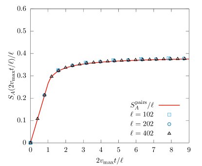
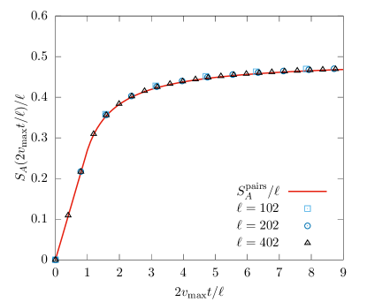
Let us start considering states (14) with ν=2𝜈2\nu=2. As noted in Section III, these states produce a distribution of excitations characterised by correlated particle-hole pairs with momenta k𝑘k and kπ𝑘𝜋k-\pi. Even if now the excitations do not have opposite momenta, the semiclassical reasoning leading to (39) can be carried out with no modifications. This is because the two particles in the pair continue to have opposite velocities. We then expect Eq. (39) to correctly reproduce the evolution of entanglement entropy from the states |Φ{a0,a1}2ketsubscriptsuperscriptΦ2subscript𝑎0subscript𝑎1\ket{\Phi^{2}_{\{a_{0},a_{1}\}}} in the scaling limit (38). This is confirmed by our numerical simulations, as demonstrated in Fig. 1 for two representative examples. In the figure we plot SA(t)/subscript𝑆𝐴𝑡S_{A}(t)/\ell as a function of 2vmaxt/2subscript𝑣max𝑡2v_{\rm max}t/\ell, where we set vmaxmaxkv(k)=2Jsubscript𝑣maxsubscript𝑘𝑣𝑘2𝐽v_{\rm max}\equiv\max_{k}v(k)=2J. The collapse of the data for increasing \ell demonstrates that they have converged to the scaling limit.
Refer to caption Refer to caption
Figure 1: Evolution of the entanglement entropy SA(t)/subscript𝑆𝐴𝑡S_{A}(t)/\ell in the rescaled time 2vmaxt/2subscript𝑣max𝑡2v_{\rm max}t/\ell (vmax=2Jsubscript𝑣max2𝐽v_{\rm max}=2J) for two different quenches from states |Φ{a0,a1}2ketsubscriptsuperscriptΦ2subscript𝑎0subscript𝑎1\ket{\Phi^{2}_{\{a_{0},a_{1}\}}} and three different subsystem lengths \ell. The figure compares the results of the numerical calculations (31) (points) with the semiclassical prediction of Eq. (39) (line). For the case reported on the left panel the parameters of the initial state are (a0,a1)=(0.88,0.48i)subscript𝑎0subscript𝑎10.880.48𝑖{(a_{0},a_{1})=(0.88,0.48i)} while for that on the right panel (a0,a1)=(1/2,ei2π10/2)subscript𝑎0subscript𝑎112superscript𝑒𝑖2𝜋102{(a_{0},a_{1})=(1/\sqrt{2},e^{-i\frac{2\pi}{10}}/\sqrt{2})}.

V.2.2 States with ν>2𝜈2\nu>2

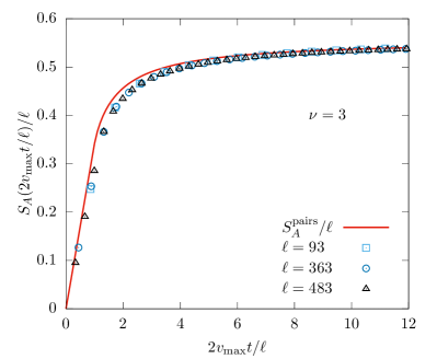
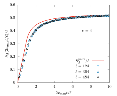
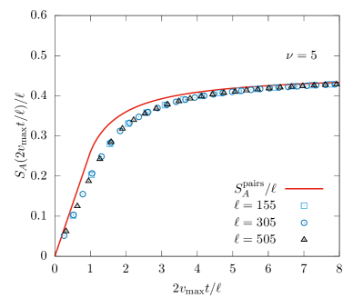
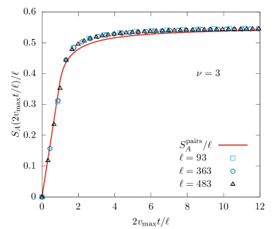
Considering instead the case ν>2𝜈2\nu>2, the situation becomes more complicated. As noted in Section III, such states impose a ν𝜈\nu-plet structure in the eigenstates of the Hamiltonian contributing to the dynamics instead of a pair one. Since there is no pair structure we have no reason to expect Eq. (39) to hold. Our numerical calculations show that, in this case, Eq. (39) does indeed not hold. This is demonstrated in Figs. 2 and 3 for four representative examples. From these figures we clearly see that the numerical data for different \ell have already reached convergence and that they show a distinct deviation from the prediction of Eq. (39). Note, however, that at infinite times the prediction of Eq. (39) seems to be recovered. This is in agreement with the widely believed equality between entanglement entropy and thermodynamic entropy at infinite times after the quench calabrese_evolution_2005 ; alba_entanglement_2016 ; dls-13 ; bam-15 ; Gur14 ; SPR11 .
Refer to caption
Refer to caption
Figure 2: Evolution of the entanglement entropy SA(t)/subscript𝑆𝐴𝑡S_{A}(t)/\ell in the rescaled time 2vmaxt/2subscript𝑣max𝑡2v_{\rm max}t/\ell (vmax=2Jsubscript𝑣max2𝐽v_{\rm max}=2J) after quenches from two different states |Φ{a0,a1,a2}3ketsubscriptsuperscriptΦ3subscript𝑎0subscript𝑎1subscript𝑎2\ket{\Phi^{3}_{\{a_{0},a_{1},a_{2}\}}} and three different subsystem-lengths \ell. The figure compares the results of the numerical calculations (31) with the semiclassical prediction of Eq. (39). For the case reported on the left panel the parameters of the initial state are (a0,a1,a2)=(0.5,0.45eiπ6,0.74ei5π7)subscript𝑎0subscript𝑎1subscript𝑎20.50.45superscript𝑒𝑖𝜋60.74superscript𝑒𝑖5𝜋7{(a_{0},a_{1},a_{2})=(0.5,0.45\,e^{-i\frac{\pi}{6}},0.74\,e^{i\frac{5\pi}{7}})} while for that on the right panel (a0,a1,a2)=(0.12,0.46eiπ6,0.88ei35π73)subscript𝑎0subscript𝑎1subscript𝑎20.120.46superscript𝑒𝑖𝜋60.88superscript𝑒𝑖35𝜋73{(a_{0},a_{1},a_{2})=(0.12,0.46\,e^{-i\frac{\pi}{6}},0.88e^{i\frac{35\pi}{73}})}.
Refer to caption
Refer to caption
Figure 3: Evolution of the entanglement entropy SA(t)/subscript𝑆𝐴𝑡S_{A}(t)/\ell in the rescaled time 2vmaxt/2subscript𝑣max𝑡2v_{\rm max}t/\ell (vmax=2Jsubscript𝑣max2𝐽v_{\rm max}=2J) after quenches from two different states |Φ{a0,a1,a2}νketsubscriptsuperscriptΦ𝜈subscript𝑎0subscript𝑎1subscript𝑎2\ket{\Phi^{\nu}_{\{a_{0},a_{1},a_{2}\}}} and three different subsystem-lengths \ell. The figure compares the results of the numerical calculations (31) with the semiclassical prediction of Eq. (39). For the case reported on the left panel the parameters of the initial state are ν=4𝜈4\nu=4 and (a0,a1,a2,a3)=(0.11,0.44ei35π6,0.85ei35π73,0.26ei3π35)subscript𝑎0subscript𝑎1subscript𝑎2subscript𝑎30.110.44superscript𝑒𝑖35𝜋60.85superscript𝑒𝑖35𝜋730.26superscript𝑒𝑖3𝜋35{(a_{0},a_{1},a_{2},a_{3})=(0.11,0.44\,e^{i\frac{35\pi}{6}},0.85\,e^{i\frac{35\pi}{73}},0.26\,e^{i\frac{3\pi}{35}})} while for that on the right panel ν=5𝜈5\nu=5 and (a0,a1,a2,a3,a4)=(0.11,0.43ei5π6,0.25ei3π35,0.82ei35π73,0.25ei3π35)subscript𝑎0subscript𝑎1subscript𝑎2subscript𝑎3subscript𝑎40.110.43superscript𝑒𝑖5𝜋60.25superscript𝑒𝑖3𝜋350.82superscript𝑒𝑖35𝜋730.25superscript𝑒𝑖3𝜋35{(a_{0},a_{1},a_{2},a_{3},a_{4})=(0.11,0.43\,e^{i\frac{5\pi}{6}},0.25\,e^{i\frac{3\pi}{35}},0.82\,e^{i\frac{35\pi}{73}},0.25\,e^{i\sqrt{\frac{3\pi}{35}}})}.

V.2.3 Generalised semiclassical formula

Our strategy here is to stick to the semiclassical picture and interpret the failure of Eq. (39) as a consequence of the absence of the pair structure. Our goal is then to derive a semi-classical formula, which takes into account the more general ν𝜈\nu-plet structure in the excitations selected by the states (14) with ν>2𝜈2\nu>2. To this aim it is convenient to introduce the following relabelling, which corresponds to a folding of the Brillouin zone. Instead of specifying the states using a single species of quasiparticles labelled by the momentum k[π,π]𝑘𝜋𝜋k\in[-\pi,\pi] we use ν𝜈\nu different species of quasiparticles with “rapidity” p[π2π/ν,π]𝑝𝜋2𝜋𝜈𝜋p\in[\pi-2\pi/\nu,\pi]. The dispersion relation of the new quasiparticles is given by

kj(p)=p2(j1)πνεj(p)=2Jcos(p2(j1)πν)j=1,,ν,formulae-sequencesubscript𝑘𝑗𝑝𝑝2𝑗1𝜋𝜈formulae-sequencesubscript𝜀𝑗𝑝2𝐽𝑝2𝑗1𝜋𝜈𝑗1𝜈k_{j}(p)=p-\frac{2(j-1)\pi}{\nu}\qquad\qquad\varepsilon_{j}(p)=2J\cos\left(p-\frac{2(j-1)\pi}{\nu}\right)\qquad\qquad j=1,\ldots,\nu\,, (42)

and their velocities

vj(p)=εj(p)kj(p)=2Jsin(p2(j1)πν)j=1,,ν.formulae-sequencesubscript𝑣𝑗𝑝subscript𝜀𝑗𝑝subscript𝑘𝑗𝑝2𝐽𝑝2𝑗1𝜋𝜈𝑗1𝜈v_{j}(p)=\frac{\partial\varepsilon_{j}(p)}{\partial k_{j}(p)}=2J\sin\left(p-\frac{2(j-1)\pi}{\nu}\right)\qquad\qquad j=1,\ldots,\nu\,. (43)

With this relabelling the eigenstates of the Hamiltonian are described in the thermodynamic limit by the following set of root densities in rapidity space

ρ(j)(p)=ρ(p2(j1)πν)p[π2π/ν,π]j=1,,ν,formulae-sequencesuperscript𝜌𝑗𝑝𝜌𝑝2𝑗1𝜋𝜈formulae-sequence𝑝𝜋2𝜋𝜈𝜋𝑗1𝜈\rho^{(j)}(p)=\rho\left(p-\frac{2(j-1)\pi}{\nu}\right)\qquad\qquad p\in\left[\pi-2\pi/\nu,\pi\right]\qquad\qquad j=1,\ldots,\nu\,, (44)

where ρ(k)𝜌𝑘\rho(k) is the root density (13). In particular we denote by {ρs(j)(p)}j=1νsuperscriptsubscriptsubscriptsuperscript𝜌𝑗𝑠𝑝𝑗1𝜈\{\rho^{(j)}_{s}(p)\}_{j=1}^{\nu} the root densities of the stationary state (24). The constraint (20) is reflected in the following condition on the root densities of the eigenstates with nonzero overlap

j=1νρ(j)(p)=12π.superscriptsubscript𝑗1𝜈superscript𝜌𝑗𝑝12𝜋\sum_{j=1}^{\nu}\rho^{(j)}(p)=\frac{1}{2\pi}\,. (45)

To find a generalisation of (39) which is able to describe the ν>2𝜈2\nu>2 case we make the following three assumptions

  • 1.

    The quench produces a ν𝜈\nu-plet of correlated excitations at every spacial point.

  • 2.

    Excitations move as free classical particles with velocities vj(p)subscript𝑣𝑗𝑝v_{j}(p).

  • 3.

    Every time that a subset of the particles of a given ν𝜈\nu-plet is in the subsystem A𝐴A and the rest is out of it, there is a nontrivial contribution to the entanglement.

The only nontrivial step we need to take in order to get a testable prediction is to determine the contribution of a given partition of the ν𝜈\nu-plet to the entanglement. We will find it by generalising (40), valid in the case ν=2𝜈2\nu=2. Let us first reconsider that case in order to develop a general strategy. We call s1(k)subscript𝑠1𝑘s_{1}(k) the contribution to the entanglement given by the pair of momentum k𝑘k with a particle of species 111 within the system and its companion of species 222 out. We call s2(k)subscript𝑠2𝑘s_{2}(k) the contribution in the reversed case of the particle of species 222 located in the system and that of species 111 out of it. Eq. (39) is obtained requiring

s1(k)=s2(k)=s(k)=12πlog12πρs(1)(k)logρs(1)(k)[12πρs(1)(k)]log[12πρs(1)(k)],k[0,π].formulae-sequencesubscript𝑠1𝑘subscript𝑠2𝑘𝑠𝑘12𝜋12𝜋subscriptsuperscript𝜌1𝑠𝑘subscriptsuperscript𝜌1𝑠𝑘delimited-[]12𝜋subscriptsuperscript𝜌1𝑠𝑘12𝜋subscriptsuperscript𝜌1𝑠𝑘𝑘0𝜋s_{1}(k)=s_{2}(k)=s(k)=\frac{1}{2\pi}\log\frac{1}{2\pi}-\rho^{(1)}_{s}(k)\log\rho^{(1)}_{s}(k)-\left[\frac{1}{2\pi}-\rho^{(1)}_{s}(k)\right]\log\left[\frac{1}{2\pi}-\rho^{(1)}_{s}(k)\right]\,,\qquad k\in[0,\pi]\,. (46)

Note that s1(k)=s2(k)subscript𝑠1𝑘subscript𝑠2𝑘s_{1}(k)=s_{2}(k) is in accordance with the basic property of bipartite entanglement: SA(t)=SA¯(t)subscript𝑆𝐴𝑡subscript𝑆¯𝐴𝑡S_{A}(t)=S_{\bar{A}}(t) where A¯¯𝐴\bar{A} is the complement of A𝐴A.

A way to explain (46) is as follows. First we interpret ρs(i)(p)subscriptsuperscript𝜌𝑖𝑠𝑝\rho^{(i)}_{s}(p) as the density of quasiparticle excitations of momentum p𝑝p and species i𝑖i produced by the quench. So that in a region of size a𝑎a

N(i)(a;p)=aρs(i)(p)dpsuperscript𝑁𝑖𝑎𝑝𝑎subscriptsuperscript𝜌𝑖𝑠𝑝d𝑝N^{(i)}(a;p)=a\rho^{(i)}_{s}(p){\rm d}p (47)

excitations of species i𝑖i and momentum in [p,p+dp]𝑝𝑝d𝑝[p,p+{\rm d}p] are produced. Second, we consider a pair of momenta p𝑝p emitted from a point x𝑥x such that only the particle of species 1 is within the system at time t𝑡t. In this case, all the quasiparticles of species 111 and momentum in [p,p+dp]𝑝𝑝d𝑝[p,p+{\rm d}p] coming from a region [xϵ/2,x+ϵ/2]𝑥italic-ϵ2𝑥italic-ϵ2[x-\epsilon\ell/2,x+\epsilon\ell/2] are in the system at time t𝑡t for small enough ϵitalic-ϵ\epsilon; those of species 2 are out of the system. This means that of the

N(p)=N(1)(ϵ,p)+N(2)(ϵ,p),𝑁𝑝superscript𝑁1italic-ϵ𝑝superscript𝑁2italic-ϵ𝑝N(p)=N^{(1)}(\epsilon\ell,p)+N^{(2)}(\epsilon\ell,p)\,, (48)

particles of momentum [p,p+dp]𝑝𝑝d𝑝[p,p+{\rm d}p] produced in [xϵ/2,x+ϵ/2]𝑥italic-ϵ2𝑥italic-ϵ2[x-\epsilon\ell/2,x+\epsilon\ell/2], Nin(p)=N(1)(ϵ,p)subscript𝑁in𝑝superscript𝑁1italic-ϵ𝑝N_{\rm in}(p)=N^{(1)}(\epsilon\ell,p) are in the system at time t𝑡t and Nout(p)=N(2)(ϵ,p)subscript𝑁out𝑝superscript𝑁2italic-ϵ𝑝N_{\rm out}(p)=N^{(2)}(\epsilon\ell,p) are out of it.

In this framework, the contribution to the entanglement entropy of the particles emitted from the region [xϵ/2,x+ϵ/2]𝑥italic-ϵ2𝑥italic-ϵ2{[x-\epsilon\ell/2,x+\epsilon\ell/2]} can be interpreted as the logarithm of the number of ways we can arrange N(p)𝑁𝑝N(p) particles in two groups of Nin(p)subscript𝑁in𝑝N_{\rm in}(p) and Nout(p)subscript𝑁out𝑝N_{\rm out}(p), divided by the size of the region. In the scaling limit (38), which we denote by limscsubscriptsc{\textstyle\lim_{\rm sc}}, we have

s1(p)dp=limsc1ϵlogN(p)!Nin(p)!Nout(p)!=s(p)dp.subscript𝑠1𝑝d𝑝subscriptsc1italic-ϵ𝑁𝑝subscript𝑁in𝑝subscript𝑁out𝑝𝑠𝑝d𝑝s_{1}(p){\rm d}p={\textstyle\lim_{\rm{sc}}}\frac{1}{\epsilon\ell}\log\frac{N(p)!}{N_{\rm in}(p)!N_{\rm out}(p)!}=s(p){\rm d}p\,. (49)

The same reasoning can be carried out also assuming that particles of species 222 are in the system at time t𝑡t and those of species 111 are out: this is realised by exchanging ρ(1)(p)superscript𝜌1𝑝\rho^{(1)}(p) and 12πρ(1)(p)12𝜋superscript𝜌1𝑝\frac{1}{2\pi}-\rho^{(1)}(p) in the formulae above. Since (49) is symmetric under this exchange, we find

s1(p)=s2(p)=s(p),p[0,π].formulae-sequencesubscript𝑠1𝑝subscript𝑠2𝑝𝑠𝑝𝑝0𝜋s_{1}(p)=s_{2}(p)=s(p)\,,\qquad p\in[0,\pi]\,. (50)

We can proceed in the same way in the generic ν𝜈\nu case. If only a subset of particles {j1,,jm}{1,,ν}subscript𝑗1subscript𝑗𝑚1𝜈\{j_{1},...,j_{m}\}\subset\{1,\ldots,\nu\} of a given ν𝜈\nu-plet are in A𝐴A at time t𝑡t, the numbers Nin(p)subscript𝑁in𝑝N_{\rm in}(p) and Nout(p)subscript𝑁out𝑝N_{\rm out}(p) read as

Nin(p)=ϵ(i=1mρs(ji)(p))dp,Nout(p)=ϵ(12πi=1mρs(ji)(p))dp.formulae-sequencesubscript𝑁in𝑝italic-ϵsuperscriptsubscript𝑖1𝑚superscriptsubscript𝜌𝑠subscript𝑗𝑖𝑝d𝑝subscript𝑁out𝑝italic-ϵ12𝜋superscriptsubscript𝑖1𝑚superscriptsubscript𝜌𝑠subscript𝑗𝑖𝑝d𝑝N_{\rm in}(p)=\epsilon\ell\left(\sum_{i=1}^{m}\rho_{s}^{(j_{i})}(p)\right){\rm d}p\,,\qquad\qquad N_{\rm out}(p)=\epsilon\ell\left(\frac{1}{2\pi}-\sum_{i=1}^{m}\rho_{s}^{(j_{i})}(p)\right){\rm d}p\,. (51)

We then postulate that the contribution to the entanglement entropy is

s{ji}(p)dpsubscript𝑠subscript𝑗𝑖𝑝d𝑝\displaystyle s_{\{j_{i}\}}(p){\rm d}p limsc1ϵlogN(p)!Nin(p)!Nout(p)!absentsubscript𝑠𝑐1italic-ϵ𝑁𝑝subscript𝑁in𝑝subscript𝑁out𝑝\displaystyle\equiv{\textstyle\lim_{sc}}\frac{1}{\epsilon\ell}\log\frac{N(p)!}{N_{\rm in}(p)!N_{\rm out}(p)!}
=[12πlog12π[i=1mρs(ji)(p)]log[i=1mρs(ji)(p)][12πi=1mρs(ji)(p)]log[12πi=1mρs(ji)(p)]]dp.absentdelimited-[]12𝜋12𝜋delimited-[]superscriptsubscript𝑖1𝑚superscriptsubscript𝜌𝑠subscript𝑗𝑖𝑝superscriptsubscript𝑖1𝑚superscriptsubscript𝜌𝑠subscript𝑗𝑖𝑝delimited-[]12𝜋superscriptsubscript𝑖1𝑚superscriptsubscript𝜌𝑠subscript𝑗𝑖𝑝12𝜋superscriptsubscript𝑖1𝑚superscriptsubscript𝜌𝑠subscript𝑗𝑖𝑝d𝑝\displaystyle=\left[\frac{1}{2\pi}\log\frac{1}{2\pi}-\left[\sum_{i=1}^{m}\rho_{s}^{(j_{i})}(p)\right]\log\left[\sum_{i=1}^{m}\rho_{s}^{(j_{i})}(p)\right]-\left[\frac{1}{2\pi}-\sum_{i=1}^{m}\rho_{s}^{(j_{i})}(p)\right]\log\left[\frac{1}{2\pi}-\sum_{i=1}^{m}\rho_{s}^{(j_{i})}(p)\right]\right]{\rm d}p\,. (52)

Note that, as a consequence of the constraint (44), this form is symmetric when exchanging {j1,,jm}subscript𝑗1subscript𝑗𝑚\{j_{1},...,j_{m}\} with its complement {1,,ν}{j1,,jm}1𝜈subscript𝑗1subscript𝑗𝑚{\{1,\ldots,\nu\}\setminus\{j_{1},...,j_{m}\}}. This is again in accordance with the basic property of bipartite entanglement.

The assumptions 1., 2., and 3., supplemented with the form (52) of the contribution, turn the problem of computing the time evolution of the entanglement entropy into a kinematic problem: we have to determine which particular bipartition of which particular ν𝜈\nu-plets contributes at each time. Before considering the problem for finite times, let us take the infinite time limit. In this limit only one particle for each correlated ν𝜈\nu-plet can be in A𝐴A, as the particles have different velocity. This means that for infinite times the entanglement entropy reads as

SA()=π2πνπj=1νsj(p)=ππsYY[ρ](k).subscript𝑆𝐴superscriptsubscript𝜋2𝜋𝜈𝜋superscriptsubscript𝑗1𝜈subscript𝑠𝑗𝑝superscriptsubscript𝜋𝜋subscript𝑠YYdelimited-[]𝜌𝑘S_{A}(\infty)=\ell\int_{\pi-\frac{2\pi}{\nu}}^{\pi}\sum_{j=1}^{\nu}s_{j}(p)=\ell\int_{-\pi}^{\pi}s_{\text{YY}}[\rho](k)\,. (53)

Namely, the entanglement entropy at infinite times is given by the thermodynamic entropy, in agreement with the general expectations Gur14 ; SPR11 and the results of Figure 2. This gives a nontrivial consistency check on the expression (52).

Let us now move to finding the entanglement entropy for finite times, for simplicity focusing on the case ν=3𝜈3\nu=3. Let us consider a fixed p𝑝p, since depending on the value of p𝑝p the velocities have a certain ordering. Let us consider the case 0<v3(p)<v2(p)<v1(p)0subscript𝑣3𝑝subscript𝑣2𝑝subscript𝑣1𝑝0<v_{3}(p)<v_{2}(p)<v_{1}(p) note . We denote by

SA(t)|p,0<v3(p)<v2(p)<v1(p)evaluated-atsubscript𝑆𝐴𝑡𝑝0subscript𝑣3𝑝subscript𝑣2𝑝subscript𝑣1𝑝S_{A}(t)|_{p,0<v_{3}(p)<v_{2}(p)<v_{1}(p)} (54)

the contribution to the entanglement in this case.
Refer to caption
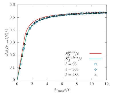
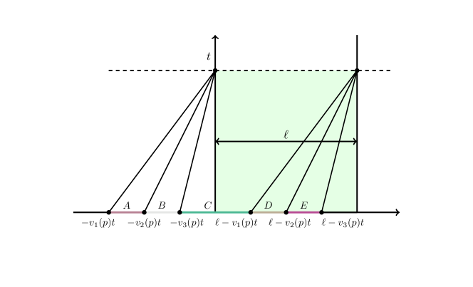
Figure 4: Regions contributing to the entanglement entropy after a quench from a state |Φ{a0,a1,a2}3ketsubscriptsuperscriptΦ3subscript𝑎0subscript𝑎1subscript𝑎2\ket{\Phi^{3}_{\{a_{0},a_{1},a_{2}\}}} for 0<v3(p)<v2(p)<v1(p)0subscript𝑣3𝑝subscript𝑣2𝑝subscript𝑣1𝑝0<v_{3}(p)<v_{2}(p)<v_{1}(p) and t</(v1(p)v3(p))𝑡subscript𝑣1𝑝subscript𝑣3𝑝t<\ell/(v_{1}(p)-v_{3}(p)).

For short enough times t𝑡t the triplets contributing to the entanglement entropy are generated in the regions depicted in Fig. 4. In particular

  • -

    No particles from the triplets generated on the left of A𝐴A or on the right of E𝐸E can be inside the system at time t𝑡t and hence contribute to the entanglement.

  • -

    Only particles of species 111 from correlated triplets generated in the region A𝐴A can be inside the system at time t𝑡t, so this region contributes with a term s1(p)(v1(p)v2(p))tsubscript𝑠1𝑝subscript𝑣1𝑝subscript𝑣2𝑝𝑡s_{1}(p)(v_{1}(p)-v_{2}(p))t.

  • -

    Only particles of species 1 and 2 from the correlated triplets generated in the region B𝐵B are within the system, so this region gives a contribution of the form s3(p)(v2(p)v3(p))tsubscript𝑠3𝑝subscript𝑣2𝑝subscript𝑣3𝑝𝑡s_{3}(p)(v_{2}(p)-v_{3}(p))t.

  • -

    All the particles from the correlated triplets created in the region C𝐶C are within the system, so there is then no contribution to the entanglement from this region.

  • -

    Only particles of species 2 and 3 from the triplets originating in D𝐷D are within the system, so we have the contribution s1(p)(v1(p)v2(p))tsubscript𝑠1𝑝subscript𝑣1𝑝subscript𝑣2𝑝𝑡s_{1}(p)(v_{1}(p)-v_{2}(p))t.

  • -

    Only particles of species 3 are within the system for the triplets originating in E𝐸E, so we have s3(p)(v2(p)v3(p))tsubscript𝑠3𝑝subscript𝑣2𝑝subscript𝑣3𝑝𝑡s_{3}(p)(v_{2}(p)-v_{3}(p))t.

The situation changes when the time becomes equal to /(v1(p)v3(p))subscript𝑣1𝑝subscript𝑣3𝑝\ell/(v_{1}(p)-v_{3}(p)), since at that time the region C𝐶C shrinks to 0, and one has to consider a configuration different from that in Fig. 4, where the regions B𝐵B and D𝐷D overlap. It is again very easy to find all the relevant contributions as we did above. Proceeding in this way, we find the entire contribution given by triplets of momentum p𝑝p can be written as

SA(t)|p,0<v3(p)<v2(p)<v1(p)=f(,t,p|3,2,1),evaluated-atsubscript𝑆𝐴𝑡𝑝0subscript𝑣3𝑝subscript𝑣2𝑝subscript𝑣1𝑝𝑓𝑡conditional𝑝321S_{A}(t)|_{p,0<v_{3}(p)<v_{2}(p)<v_{1}(p)}=f(\ell,t,p|3,2,1)\,, (55)

where we introduced the function

f(,t,p|a,b,c)𝑓𝑡conditional𝑝𝑎𝑏𝑐absent\displaystyle f(\ell,t,p|a,b,c)\equiv
2t[sa(p)(vb(p)va(p))+sc(p)(vc(p)vb(p))]θ(τca(p)t)2𝑡delimited-[]subscript𝑠𝑎𝑝subscript𝑣𝑏𝑝subscript𝑣𝑎𝑝subscript𝑠𝑐𝑝subscript𝑣𝑐𝑝subscript𝑣𝑏𝑝𝜃subscript𝜏𝑐𝑎𝑝𝑡\displaystyle 2t\Bigl{[}s_{a}(p)(v_{b}(p)-v_{a}(p))+s_{c}(p)(v_{c}(p)-v_{b}(p))\Bigr{]}\theta\left(\tau_{ca}(p)-t\right)
+[sa(p)((va(p)2vb(p)+vc(p))t)+sb(p)(((vc(p)va(p))t)\displaystyle+\Bigl{[}s_{a}(p)(\ell-(v_{a}(p)-2v_{b}(p)+v_{c}(p))t)+s_{b}(p)(((v_{c}(p)-v_{a}(p))t-\ell)
+sc(p)(+(va(p)2vb(p)+vc(p))t)]χt([τca(p),min[τba(p),τcb(p)]])\displaystyle\qquad+s_{c}(p)(\ell+(v_{a}(p)-2v_{b}(p)+v_{c}(p))t)\Bigr{]}\chi_{t}\left(\left[\tau_{ca}(p),\min\left[\tau_{ba}(p),\tau_{cb}(p)\right]\right]\right)
+θ(τcb(p)τba(p))[sa(p)(2+(vb(p)vc(p))t)+(sb(p)+sc(p))(vc(p)vb(p))t]χt([τba(p),τcb(p)])𝜃subscript𝜏𝑐𝑏𝑝subscript𝜏𝑏𝑎𝑝delimited-[]subscript𝑠𝑎𝑝2subscript𝑣𝑏𝑝subscript𝑣𝑐𝑝𝑡subscript𝑠𝑏𝑝subscript𝑠𝑐𝑝subscript𝑣𝑐𝑝subscript𝑣𝑏𝑝𝑡subscript𝜒𝑡subscript𝜏𝑏𝑎𝑝subscript𝜏𝑐𝑏𝑝\displaystyle+\theta(\tau_{cb}(p)-\tau_{ba}(p))\Bigl{[}s_{a}(p)(2\ell+(v_{b}(p)-v_{c}(p))t)+(s_{b}(p)+s_{c}(p))(v_{c}(p)-v_{b}(p))t\Bigr{]}\chi_{t}\left(\left[\tau_{ba}(p),\tau_{cb}(p)\right]\right)
+θ(τba(p)τcb(p))[sc(p)(2+(va(p)vb(p))t)+(sb(p)+sa(p))(vb(p)va(p))t]χt([τcb(p),τba(p)])𝜃subscript𝜏𝑏𝑎𝑝subscript𝜏𝑐𝑏𝑝delimited-[]subscript𝑠𝑐𝑝2subscript𝑣𝑎𝑝subscript𝑣𝑏𝑝𝑡subscript𝑠𝑏𝑝subscript𝑠𝑎𝑝subscript𝑣𝑏𝑝subscript𝑣𝑎𝑝𝑡subscript𝜒𝑡subscript𝜏𝑐𝑏𝑝subscript𝜏𝑏𝑎𝑝\displaystyle+\theta(\tau_{ba}(p)-\tau_{cb}(p))\Bigl{[}s_{c}(p)(2\ell+(v_{a}(p)-v_{b}(p))t)+(s_{b}(p)+s_{a}(p))(v_{b}(p)-v_{a}(p))t\Bigr{]}\chi_{t}\left(\left[\tau_{cb}(p),\tau_{ba}(p)\right]\right)
+[sa(p)+sb(p)+sc(p)]θ(tmax[τba(p),τcb(p)]).delimited-[]subscript𝑠𝑎𝑝subscript𝑠𝑏𝑝subscript𝑠𝑐𝑝𝜃𝑡subscript𝜏𝑏𝑎𝑝subscript𝜏𝑐𝑏𝑝\displaystyle+\ell\Bigl{[}s_{a}(p)+s_{b}(p)+s_{c}(p)\Bigr{]}\theta\left(t-\max\left[\tau_{ba}(p),\tau_{cb}(p)\right]\right)\,. (56)

Here χx([a,b])subscript𝜒𝑥𝑎𝑏\chi_{x}([a,b]) is the characteristic function of the interval [a,b]𝑎𝑏[a,b] and we defined

τij(p)vi(p)vj(p).subscript𝜏𝑖𝑗𝑝subscript𝑣𝑖𝑝subscript𝑣𝑗𝑝\tau_{ij}(p)\equiv\frac{\ell}{v_{i}(p)-v_{j}(p)}\,. (57)

In general, proceeding as above, we see that if the velocities have the ordering vσ(3)(p)<vσ(2)(p)<vσ(1)(p)subscript𝑣𝜎3𝑝subscript𝑣𝜎2𝑝subscript𝑣𝜎1𝑝v_{\sigma(3)}(p)<v_{\sigma(2)}(p)<v_{\sigma(1)}(p), where σ𝜎\sigma is a generic permutation in 𝒮3subscript𝒮3\mathcal{S}_{3}, the contribution to the entanglement entropy is given by

SA(t)|p,vσ(3)(p)<vσ(2)(p)<vσ(1)(p)=f(,t,p|σ(3),σ(2),σ(1)).evaluated-atsubscript𝑆𝐴𝑡𝑝subscript𝑣𝜎3𝑝subscript𝑣𝜎2𝑝subscript𝑣𝜎1𝑝𝑓𝑡conditional𝑝𝜎3𝜎2𝜎1S_{A}(t)|_{p,v_{\sigma(3)}(p)<v_{\sigma(2)}(p)<v_{\sigma(1)}(p)}=f(\ell,t,p|\sigma(3),\sigma(2),\sigma(1))\,. (58)

We can then write the total entanglement entropy as follows

SAtriplets(t)=subscriptsuperscript𝑆triplets𝐴𝑡absent\displaystyle S^{\rm triplets}_{A}(t)= σ𝒮3π/3πdpθ(vσ(3)<vσ(2)(p)<vσ(1)(p))f(,t,p|σ(3),σ(2),σ(1)).subscript𝜎subscript𝒮3superscriptsubscript𝜋3𝜋differential-d𝑝𝜃subscript𝑣𝜎3subscript𝑣𝜎2𝑝subscript𝑣𝜎1𝑝𝑓𝑡conditional𝑝𝜎3𝜎2𝜎1\displaystyle\sum_{\sigma\in\mathcal{S}_{3}}\,\int_{\pi/3}^{\pi}\!\!\!{\rm d}p\,\,\theta(v_{\sigma(3)}<v_{\sigma(2)}(p)<v_{\sigma(1)}(p))\,\,f(\ell,t,p|\sigma(3),\sigma(2),\sigma(1))\,. (59)

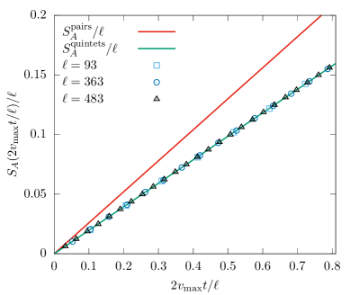
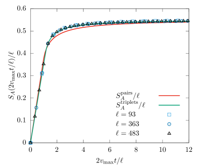
In Fig. 5 we compare the prediction of (59) with the numerical calculations for increasing \ell in two representative examples. As we see from the plot, the agreement is extremely convincing.
Refer to caption
Refer to caption
Figure 5: Evolution of the entanglement entropy SA(t)/subscript𝑆𝐴𝑡S_{A}(t)/\ell in the rescaled time 2vmaxt/2subscript𝑣max𝑡2v_{\rm max}t/\ell (vmax=2Jsubscript𝑣max2𝐽{v_{\rm max}=2J}) after quenches from two different states |Φ{a0,a1,a2}3ketsubscriptsuperscriptΦ3subscript𝑎0subscript𝑎1subscript𝑎2\ket{\Phi^{3}_{\{a_{0},a_{1},a_{2}\}}} and three different subsystem-lengths \ell. The figure compares the results of the numerical calculations with the semiclassical predictions of Eq. (39) and of Eq. (59). For the case reported on the left panel the parameters of the initial state are (a0,a1,a2)=(0.5,0.45eiπ6,0.74ei5π7)subscript𝑎0subscript𝑎1subscript𝑎20.50.45superscript𝑒𝑖𝜋60.74superscript𝑒𝑖5𝜋7{(a_{0},a_{1},a_{2})=(0.5,0.45\,e^{-i\frac{\pi}{6}},0.74\,e^{i\frac{5\pi}{7}})} while for that on the right panel (a0,a1,a2)=(0.12,0.46eiπ6,0.88ei35π73)subscript𝑎0subscript𝑎1subscript𝑎20.120.46superscript𝑒𝑖𝜋60.88superscript𝑒𝑖35𝜋73{(a_{0},a_{1},a_{2})=(0.12,0.46\,e^{-i\frac{\pi}{6}},0.88e^{i\frac{35\pi}{73}})}.

The explicit expression for generic ν𝜈\nu is obtained reasoning in the same way, but it rapidly becomes quite cumbersome as there are many possible orderings for the τij(p)subscript𝜏𝑖𝑗𝑝\tau_{ij}(p). Here we give the result in the simplifying limit of \ell\rightarrow\infty, i.e., when the system A𝐴A corresponds to the positive real half line

limSAν-plets(t)=subscriptsubscriptsuperscript𝑆𝜈-plets𝐴𝑡absent\displaystyle\lim_{\ell\rightarrow\infty}S^{\nu{\text{-plets}}}_{A}(t)= σ𝒮νπ2π/νπdpθ(vσ(ν)<<vσ(1)(p))limf(,t,p|σ(ν),,σ(1)),subscript𝜎subscript𝒮𝜈superscriptsubscript𝜋2𝜋𝜈𝜋differential-d𝑝𝜃subscript𝑣𝜎𝜈subscript𝑣𝜎1𝑝subscript𝑓𝑡conditional𝑝𝜎𝜈𝜎1\displaystyle\sum_{\sigma\in\mathcal{S}_{\nu}}\,\int_{\pi-2\pi/\nu}^{\pi}\!\!\!{\rm d}p\,\,\theta(v_{\sigma(\nu)}<\dots<v_{\sigma(1)}(p))\,\,\lim_{\ell\rightarrow\infty}f(\ell,t,p|\sigma(\nu),\ldots,\sigma(1))\,, (60)

where

limf(,t,p|aν,,a1)=2tj=1ν1s{a1aj}(p)(vaj(p)vaj+1(p)).subscript𝑓𝑡conditional𝑝subscript𝑎𝜈subscript𝑎12𝑡superscriptsubscript𝑗1𝜈1subscript𝑠subscript𝑎1subscript𝑎𝑗𝑝subscript𝑣subscript𝑎𝑗𝑝subscript𝑣subscript𝑎𝑗1𝑝\lim_{\ell\rightarrow\infty}f(\ell,t,p|a_{\nu},\ldots,a_{1})=2t\sum_{j=1}^{\nu-1}s_{\{a_{1}\dots a_{j}\}}(p)(v_{a_{j}}(p)-v_{a_{j+1}}(p))\,. (61)

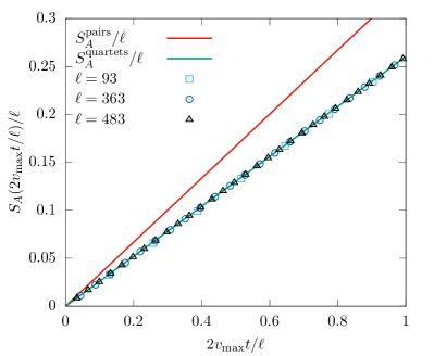
Formula (60) describes the behaviour of the entanglement entropy even at finite \ell, for times t<minijminpτij(p)𝑡subscript𝑖𝑗subscript𝑝subscript𝜏𝑖𝑗𝑝t<\min_{ij}\min_{p}{\tau_{ij}(p)}. In Fig. 6 we compare the prediction of (60) with the numerical simulations, the agreement is again excellent and gives a further confirmation of the validity of Eq. (52).
Refer to caption
Refer to caption
Figure 6: Evolution of the entanglement entropy SA(t)/subscript𝑆𝐴𝑡S_{A}(t)/\ell in the rescaled time 2vmaxt/2subscript𝑣max𝑡2v_{\rm max}t/\ell (vmax=2Jsubscript𝑣max2𝐽{v_{\rm max}=2J}) after quenches from two different states |Φ{a0,a1,a2}νketsubscriptsuperscriptΦ𝜈subscript𝑎0subscript𝑎1subscript𝑎2\ket{\Phi^{\nu}_{\{a_{0},a_{1},a_{2}\}}} and three different subsystem-lengths \ell. The figure compares the results of the numerical calculations with the semiclassical predictions of Eq. (39) and of Eq. (60), the latter is valid only for short times. For the case reported on the left panel the parameters of the initial state are ν=4𝜈4\nu=4 and (a0,a1,a2,a3)=(0.11,0.44ei35π6,0.85ei35π73,0.26ei3π35)subscript𝑎0subscript𝑎1subscript𝑎2subscript𝑎30.110.44superscript𝑒𝑖35𝜋60.85superscript𝑒𝑖35𝜋730.26superscript𝑒𝑖3𝜋35{(a_{0},a_{1},a_{2},a_{3})=(0.11,0.44\,e^{i\frac{35\pi}{6}},0.85\,e^{i\frac{35\pi}{73}},0.26\,e^{i\frac{3\pi}{35}})} while for that on the right panel ν=5𝜈5\nu=5 and (a0,a1,a2,a3,a4)=(0.11,0.43ei5π6,0.25ei3π35,0.82ei35π73,0.25ei3π35)subscript𝑎0subscript𝑎1subscript𝑎2subscript𝑎3subscript𝑎40.110.43superscript𝑒𝑖5𝜋60.25superscript𝑒𝑖3𝜋350.82superscript𝑒𝑖35𝜋730.25superscript𝑒𝑖3𝜋35{(a_{0},a_{1},a_{2},a_{3},a_{4})=(0.11,0.43\,e^{i\frac{5\pi}{6}},0.25\,e^{i\frac{3\pi}{35}},0.82\,e^{i\frac{35\pi}{73}},0.25\,e^{i\sqrt{\frac{3\pi}{35}}})}.

VI Diagonal vs Thermodynamic Entropies

In this section we investigate the relation between the stationary values reached by the entanglement entropy, coinciding with those of the thermodynamic entropy of the stationary state (24), and the recently proposed diagonal entropy P:diagonalentropy . The latter quantity is regarded as an alternative microscopic definition of the entropy of a quantum system out of equilibrium and is given by the von Neumann entropy of the diagonal ensemble, namely

Sd=Tr𝝆dlog𝝆d,subscript𝑆dTrsubscript𝝆dsubscript𝝆dS_{\rm d}=-{\rm Tr}\boldsymbol{\rho}_{\rm d}\log\boldsymbol{\rho}_{\rm d}\,, (62)

where

𝝆d=n=0k1<<kn|Ψn(k1,,kn)|Φ{am}ν|2|Ψn(k1,,kn)Ψn(k1,,kn)|,subscript𝝆dsuperscriptsubscript𝑛0subscriptsubscript𝑘1subscript𝑘𝑛superscriptinner-productsubscriptΨ𝑛subscript𝑘1subscript𝑘𝑛subscriptsuperscriptΦ𝜈subscript𝑎𝑚2ketsubscriptΨ𝑛subscript𝑘1subscript𝑘𝑛brasubscriptΨ𝑛subscript𝑘1subscript𝑘𝑛\boldsymbol{\rho}_{\rm d}=\sum_{n=0}^{\infty}\sum_{k_{1}<\ldots<k_{n}}|\braket{\Psi_{n}(k_{1},\ldots,k_{n})}{\Phi^{\nu}_{\{a_{m}\}}}|^{2}\ket{\Psi_{n}(k_{1},\ldots,k_{n})}\bra{\Psi_{n}(k_{1},\ldots,k_{n})}\,, (63)

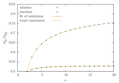
and {|Ψn(k1,,kn)}ketsubscriptΨ𝑛subscript𝑘1subscript𝑘𝑛\{\ket{\Psi_{n}(k_{1},\ldots,k_{n})}\} are the eigenstates (10) of the Hamiltonian. The quantity (62) has the important advantage of being time independent: it can be calculated on the initial state without solving the intricate many-body dynamics. The relation between Sdsubscript𝑆dS_{\rm d} and the thermodynamic entropy Sthsubscript𝑆thS_{\rm th} has recently attracted considerable attention leda-2014 ; kormos-2014 ; SPR11 ; collura-2014 ; Gur14 ; F:finitesize ; PVCR17 ; SPR:pre ; P:diagonalentropy ; D:escort ; ac-17b . While it has been suggested that these two quantities are equivalent for generic systems P:diagonalentropy , all the cases examined in the context of integrable models revealed that the diagonal entropy was half of the thermodynamic one leda-2014 ; kormos-2014 ; collura-2014 ; Gur14 ; F:finitesize ; PVCR17 ; SPR:pre ; D:escort . The latter fact is connected with the pair structure in the eigenstates contributing to the dynamics: if in an integrable model the relevant eigenstates have the pair structure then the diagonal entropy is half of the thermodynamic one, as recently shown in Ref. ac-17b . Here we show that in the absence of the pair structure the ratio of Sdsubscript𝑆dS_{\rm d} and Sthsubscript𝑆thS_{\rm th} is generically different from one and depends on the details of the initial state. Specifically, while for ν=2𝜈2\nu=2 the ratio is fixed to 1/2121/2 in agreement with the result of Ref. ac-17b , for ν>2𝜈2\nu>2 the ratio depends on the details of the states, i.e., on the configuration of {ai}subscript𝑎𝑖\{a_{i}\}. We identify the range in which the ratio varies determining a maximum and a minimum value, rmax(ν)subscript𝑟max𝜈r_{\rm max}(\nu) and rmin(ν)subscript𝑟min𝜈r_{\rm min}(\nu), as a function of ν𝜈\nu. Moreover, we show that 1/2<rmin(ν)<rmax(ν)<112subscript𝑟min𝜈subscript𝑟max𝜈11/2<r_{\rm min}(\nu)<r_{\rm max}(\nu)<1 for any finite ν𝜈\nu and limνrmax(ν)=1subscript𝜈subscript𝑟max𝜈1\lim_{\nu\rightarrow\infty}r_{\rm max}(\nu)=1, while rmin(ν)subscript𝑟min𝜈r_{\rm min}(\nu) appears to approach a constant c0.53𝑐0.53c\approx 0.53.

We begin by expressing the densities of thermodynamic entropy and diagonal entropy in the thermodynamic limit in terms of the root densities (44) of the stationary state. The thermodynamic entropy density is given by the integral of the Yang-Yang entropy. In terms of {ρ(j)(p)}j=1νsuperscriptsubscriptsuperscript𝜌𝑗𝑝𝑗1𝜈\{\rho^{(j)}(p)\}_{j=1}^{\nu} (cf. (44)) it reads as

SYY[{ρ(j)}]=log12πj=1νπ2πνπdk{ρ(j)(k)logρ(j)(k)+[12πρ(j)(k)]log[12πρ(j)(k)]}.subscript𝑆YYdelimited-[]superscript𝜌𝑗12𝜋superscriptsubscript𝑗1𝜈superscriptsubscript𝜋2𝜋𝜈𝜋differential-d𝑘superscript𝜌𝑗𝑘superscript𝜌𝑗𝑘delimited-[]12𝜋superscript𝜌𝑗𝑘12𝜋superscript𝜌𝑗𝑘S_{\mathrm{YY}}[\{\rho^{(j)}\}]=\log\frac{1}{2\pi}-\sum_{j=1}^{\nu}\int_{\pi-\frac{2\pi}{\nu}}^{\pi}\mathrm{d}k\left\{\rho^{(j)}(k)\log\rho^{(j)}(k)+\left[\frac{1}{2\pi}-\rho^{(j)}(k)\right]\log\left[\frac{1}{2\pi}-\rho^{(j)}(k)\right]\right\}\,. (64)

As shown in ac-17b , the thermodynamic limit of the diagonal entropy density is given by the reduced entropy appearing in the Quench Action approach QA ; caux_qareview and defined as the Yang-Yang entropy density reduced to the states having nonzero overlap with the initial state. In our case, the reduced entropy was determined in previousepisode and reads as

Sred[{ρ(j)}]=1νlog12πj=1νπ2πνπdkρ(j)(k)logρ(j)(k).subscript𝑆reddelimited-[]superscript𝜌𝑗1𝜈12𝜋superscriptsubscript𝑗1𝜈superscriptsubscript𝜋2𝜋𝜈𝜋differential-d𝑘superscript𝜌𝑗𝑘superscript𝜌𝑗𝑘S_{\mathrm{red}}[\{\rho^{(j)}\}]=\frac{1}{\nu}\log\frac{1}{2\pi}-\sum_{j=1}^{\nu}\int_{\pi-\frac{2\pi}{\nu}}^{\pi}\mathrm{d}k\,\rho^{(j)}(k)\log\rho^{(j)}(k)\,. (65)

Our quantity of interest can then be written as

r(ν;{ai})𝑟𝜈subscript𝑎𝑖\displaystyle r(\nu;\{a_{i}\}) SdSth=Sred[{ρs(j)}]SYY[{ρs(j)}]absentsubscript𝑆dsubscript𝑆thsubscript𝑆reddelimited-[]subscriptsuperscript𝜌𝑗𝑠subscript𝑆YYdelimited-[]subscriptsuperscript𝜌𝑗𝑠\displaystyle\equiv\frac{S_{\rm d}}{S_{\rm th}}=\frac{S_{\mathrm{red}}[\{\rho^{(j)}_{s}\}]}{S_{\mathrm{YY}}[\{\rho^{(j)}_{s}\}]}
=1νlog12ππ2πνπdkj=1νρs(j)(k)logρs(j)(k)log12ππ2πνπdkj=1ν[ρs(j)(k)logρs(j)(k)+(12πρs(j)(k))log(12πρs(j)(k))],absent1𝜈12𝜋superscriptsubscript𝜋2𝜋𝜈𝜋differential-d𝑘superscriptsubscript𝑗1𝜈subscriptsuperscript𝜌𝑗𝑠𝑘subscriptsuperscript𝜌𝑗𝑠𝑘12𝜋superscriptsubscript𝜋2𝜋𝜈𝜋differential-d𝑘superscriptsubscript𝑗1𝜈delimited-[]subscriptsuperscript𝜌𝑗𝑠𝑘subscriptsuperscript𝜌𝑗𝑠𝑘12𝜋subscriptsuperscript𝜌𝑗𝑠𝑘12𝜋subscriptsuperscript𝜌𝑗𝑠𝑘\displaystyle=\frac{\frac{1}{\nu}\log\frac{1}{2\pi}-\int_{\pi-\frac{2\pi}{\nu}}^{\pi}\mathrm{d}k\sum_{j=1}^{\nu}\rho^{(j)}_{s}(k)\log\rho^{(j)}_{s}(k)}{\log\frac{1}{2\pi}-\int_{\pi-\frac{2\pi}{\nu}}^{\pi}\mathrm{d}k\sum_{j=1}^{\nu}\left[\rho^{(j)}_{s}(k)\log\rho^{(j)}_{s}(k)+(\frac{1}{2\pi}-\rho^{(j)}_{s}(k))\log(\frac{1}{2\pi}-\rho^{(j)}_{s}(k))\right]}\,, (66)

where we explicitly reported the dependence of r𝑟r on ν𝜈\nu and {ai}subscript𝑎𝑖\{a_{i}\}. Using the constraint (45) it is immediate to show that for ν=2𝜈2\nu=2

0πdkj=12ρs(j)(k)logρs(j)(k)=120πdkj=12{ρs(j)(k)logρs(j)(k)+(12πρs(j)(k))log(12πρs(j)(k))},superscriptsubscript0𝜋differential-d𝑘superscriptsubscript𝑗12subscriptsuperscript𝜌𝑗𝑠𝑘subscriptsuperscript𝜌𝑗𝑠𝑘12superscriptsubscript0𝜋differential-d𝑘superscriptsubscript𝑗12subscriptsuperscript𝜌𝑗𝑠𝑘subscriptsuperscript𝜌𝑗𝑠𝑘12𝜋subscriptsuperscript𝜌𝑗𝑠𝑘12𝜋subscriptsuperscript𝜌𝑗𝑠𝑘\int_{0}^{\pi}\mathrm{d}k\sum_{j=1}^{2}\rho^{(j)}_{s}(k)\log\rho^{(j)}_{s}(k)=\frac{1}{2}\int_{0}^{\pi}\mathrm{d}k\sum_{j=1}^{2}\left\{\rho^{(j)}_{s}(k)\log\rho^{(j)}_{s}(k)+\left(\frac{1}{2\pi}-\rho^{(j)}_{s}(k)\right)\log\left(\frac{1}{2\pi}-\rho^{(j)}_{s}(k)\right)\right\}\,, (67)

which implies

r(2;{ai})=12,a0,a1.𝑟2subscript𝑎𝑖12for-allsubscript𝑎0subscript𝑎1r(2;\{a_{i}\})=\frac{1}{2}\,,\qquad\forall\,a_{0},\,a_{1}\,. (68)

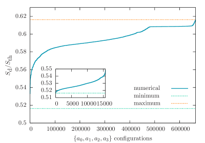
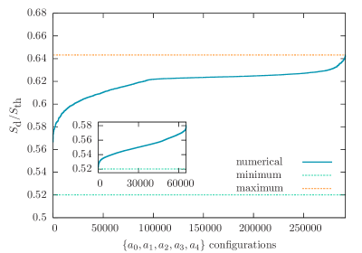
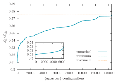
For ν>2𝜈2\nu>2, on the other hand, the ratio (66) depends explicitly on {ai}subscript𝑎𝑖\{a_{i}\}. This is demonstrated in Figs. 7, 8, and 9, where we plot the different values of the ratio obtained by sampling many different configurations of {ai}subscript𝑎𝑖\{a_{i}\}, for ν=3,4,𝜈34\nu=3,4, and 555 respectively. To perform the sampling, it is useful to explicitly solve the constraint in Eq. (14) writing the moduli of the {ai}subscript𝑎𝑖\{a_{i}\} in polar coordinates and removing a redundant global phase. For example for ν=3𝜈3\nu=3, we write the parameters as

a0subscript𝑎0\displaystyle a_{0} =cos(θ1),absentsubscript𝜃1\displaystyle=\cos(\theta_{1}), a1subscript𝑎1\displaystyle a_{1} =sin(θ1)cos(θ2)eiα1,absentsubscript𝜃1subscript𝜃2superscript𝑒isubscript𝛼1\displaystyle=\sin(\theta_{1})\cos(\theta_{2})e^{\mathrm{i}\alpha_{1}}, a2subscript𝑎2\displaystyle a_{2} =sin(θ1)sin(θ2)eiα2,absentsubscript𝜃1subscript𝜃2superscript𝑒isubscript𝛼2\displaystyle=\sin(\theta_{1})\sin(\theta_{2})e^{\mathrm{i}\alpha_{2}}, θi[0,π/2]subscript𝜃𝑖0𝜋2\displaystyle\theta_{i}\in[0,\pi/2] ,αi[0,2π).\displaystyle,\ \alpha_{i}\in[0,2\pi)\,. (69)

This allows us to simply sample the parameters at regular intervals in their allowed range.
Refer to caption
Figure 7: Here we give numerical values for the ratio of the diagonal and thermodynamic entropies in the steady state (24) for ν=3𝜈3\nu=3. We parametrised the complex constants aisubscript𝑎𝑖a_{i} as in equation (69). The larger plot evaluates the ratio for values of the aisubscript𝑎𝑖a_{i} obtained by taking all combinations of θi=0,π/20,,π/2subscript𝜃𝑖0𝜋20𝜋2\theta_{i}=0,\pi/20,\ldots,\pi/2, αi=0,π/20,,39π/20subscript𝛼𝑖0𝜋2039𝜋20\alpha_{i}=0,\pi/20,\ldots,39\pi/20 and i=1,2𝑖12i=1,2 which give unique ordered sets {a0,a1,a2}subscript𝑎0subscript𝑎1subscript𝑎2\{a_{0},a_{1},a_{2}\}. To demonstrate values closer to the minimum, we took a finer mesh around the values of the minimum: all combinations for θi=θimin0.1subscript𝜃𝑖superscriptsubscript𝜃𝑖min0.1\theta_{i}=\theta_{i}^{\text{min}}-0.1, θimin0.075superscriptsubscript𝜃𝑖min0.075\theta_{i}^{\text{min}}-0.075, …, θimin+0.1superscriptsubscript𝜃𝑖min0.1\theta_{i}^{\text{min}}+0.1 and similarly for the αisubscript𝛼𝑖\alpha_{i}. The dashed maximum value is given by the formula (75) and the minimum value in Table 1.
Refer to caption
Figure 8: Here we give numerical values for the ratio of the diagonal and thermodynamic entropies in the steady state (24) for ν=4𝜈4\nu=4. We parametrised the complex constants aisubscript𝑎𝑖a_{i} using polar coordinates for the modulus (in terms of angles θisubscript𝜃𝑖\theta_{i}) and denoting the argument as αisubscript𝛼𝑖\alpha_{i}. The larger plot evaluates the ratio for values of the aisubscript𝑎𝑖a_{i} obtained by taking all combinations of θi=0,π/10,,π/2subscript𝜃𝑖0𝜋10𝜋2\theta_{i}=0,\pi/10,\ldots,\pi/2, αi=0,π/10,,19π/10subscript𝛼𝑖0𝜋1019𝜋10\alpha_{i}=0,\pi/10,\ldots,19\pi/10 and i=1,2,3𝑖123i=1,2,3 which give unique ordered sets {a0,a1,a2,a3}subscript𝑎0subscript𝑎1subscript𝑎2subscript𝑎3\{a_{0},a_{1},a_{2},a_{3}\}. To demonstrate values closer to the minimum, we took a finer mesh around the values of the minimum: all combinations for θi=θimin0.1subscript𝜃𝑖superscriptsubscript𝜃𝑖min0.1\theta_{i}=\theta_{i}^{\text{min}}-0.1, θi=θimin0.05subscript𝜃𝑖superscriptsubscript𝜃𝑖min0.05\theta_{i}=\theta_{i}^{\text{min}}-0.05, …, θimin+0.1superscriptsubscript𝜃𝑖min0.1\theta_{i}^{\text{min}}+0.1 and similarly for the αisubscript𝛼𝑖\alpha_{i}. The dashed maximum value is given by the formula (75) and the minimum value in Table 1.
Refer to caption
Figure 9: Here we give numerical values for the ratio of the diagonal and thermodynamic entropies in the steady state (24) for ν=5𝜈5\nu=5. We parametrised the complex constants aisubscript𝑎𝑖a_{i} using polar coordinates for the modulus (in terms of angles θisubscript𝜃𝑖\theta_{i}) and denoting the argument as αisubscript𝛼𝑖\alpha_{i}. The larger plot evaluates the ratio for values of the aisubscript𝑎𝑖a_{i} obtained by taking all combinations of θi=0,π/6,π/3,π/2subscript𝜃𝑖0𝜋6𝜋3𝜋2\theta_{i}=0,\pi/6,\pi/3,\pi/2, αi=0,π/5,,9π/5subscript𝛼𝑖0𝜋59𝜋5\alpha_{i}=0,\pi/5,\ldots,9\pi/5 and i=1,2,3,4𝑖1234i=1,2,3,4 which give unique ordered sets {ai}i=04superscriptsubscriptsubscript𝑎𝑖𝑖04\{a_{i}\}_{i=0}^{4}. To demonstrate values closer to the minimum, we took a finer mesh around the values of the minimum: all combinations for θi=θimin0.15subscript𝜃𝑖superscriptsubscript𝜃𝑖min0.15\theta_{i}=\theta_{i}^{\text{min}}-0.15, θimin0.05superscriptsubscript𝜃𝑖min0.05\theta_{i}^{\text{min}}-0.05, θimin+0.05superscriptsubscript𝜃𝑖min0.05\theta_{i}^{\text{min}}+0.05, θimin+0.15superscriptsubscript𝜃𝑖min0.15\theta_{i}^{\text{min}}+0.15 and similarly for the αisubscript𝛼𝑖\alpha_{i}. The dashed maximum value is given by the formula (75) and the minimum value in Table 1.

From the plots we see that the values of r(ν;{ai})𝑟𝜈subscript𝑎𝑖r(\nu;\{a_{i}\}) are distributed between a maximum and a minimum, rmax(ν)subscript𝑟max𝜈r_{\rm max}(\nu) and rmin(ν)subscript𝑟min𝜈r_{\rm min}(\nu), which are both larger than 1/2121/2 and smaller than 111. To determine such maxima and minima analytically, one should extremise r(ν;{ai})𝑟𝜈subscript𝑎𝑖r(\nu;\{a_{i}\}) as a function of the parameters {ai}subscript𝑎𝑖\{a_{i}\} with the constraint in Eq. (14). This problem is not analytically tractable, but some analytical understanding can still be gained. It is convenient to consider the following functional

R[ν;{ρ(j)}]=Sred[{ρ(j)}]SYY[{ρ(j)}],𝑅𝜈superscript𝜌𝑗subscript𝑆reddelimited-[]superscript𝜌𝑗subscript𝑆YYdelimited-[]superscript𝜌𝑗R[\nu;\{\rho^{(j)}\}]=\frac{S_{\mathrm{red}}[\{\rho^{(j)}\}]}{S_{\mathrm{YY}}[\{\rho^{(j)}\}]}\,, (70)

together with the constraint

j=1νρ(j)(k)=12π.superscriptsubscript𝑗1𝜈superscript𝜌𝑗𝑘12𝜋\sum_{j=1}^{\nu}\rho^{(j)}(k)=\frac{1}{2\pi}\,. (71)

In Appendix C we show that the set of root densities

ρ(j)(k)=12πν,j=1,,ν,formulae-sequencesuperscript𝜌𝑗𝑘12𝜋𝜈𝑗1𝜈\rho^{(j)}(k)=\frac{1}{2\pi\nu}\,,\qquad\qquad\qquad j=1,\ldots,\nu\,, (72)

is a local maximum for the functional. These functions correspond to {ρs(j)(k)}subscriptsuperscript𝜌𝑗𝑠𝑘\{\rho^{(j)}_{s}(k)\} with

aj=eiϕandai=0ijforj=0,,ν1,ϕ,formulae-sequencesubscript𝑎𝑗superscript𝑒𝑖italic-ϕandformulae-sequencesubscript𝑎𝑖0formulae-sequencefor-all𝑖𝑗forformulae-sequence𝑗0𝜈1italic-ϕa_{j}=e^{i\phi}\qquad\text{and}\qquad a_{i}=0\qquad\forall\,i\neq j\qquad\text{for}\qquad j=0,\ldots,\nu-1\,,\qquad\phi\in\mathbb{R}\,, (73)

cf. Eq. (24). This means that (71) is also a local maximum for r(ν;{ai})𝑟𝜈subscript𝑎𝑖r(\nu;\{a_{i}\}). The value of the ratio at the point (73) reads as

r(ν)r(ν;{0,,0,eiϕj,0,,0})=logννlogν(ν1)log(ν1),j=1,,ν,ϕ.formulae-sequencesubscript𝑟𝜈𝑟𝜈subscript00superscript𝑒𝑖italic-ϕ𝑗00𝜈𝜈𝜈𝜈1𝜈1formulae-sequencefor-all𝑗1𝜈for-allitalic-ϕr_{*}(\nu)\equiv r(\nu;\{\underbrace{0,\ldots,0,e^{i\phi}}_{j},0,\ldots,0\})=\frac{\log\nu}{\nu\log\nu-(\nu-1)\log(\nu-1)}\,,\qquad\forall\,j=1,\ldots,\nu\,,\qquad\forall\,\phi\in\mathbb{R}\,. (74)

Numerical maximisation in Mathematica of the function r(ν;{ai})𝑟𝜈subscript𝑎𝑖r(\nu;\{a_{i}\}) for ν=3,,20𝜈320\nu=3,\ldots,20 gives values coinciding with this formula, see Fig. 10. Furthermore, a numerical sweep across the possible initial states for ν=3,4,5𝜈345\nu=3,4,5 (see Figures 7, 8 and 9, respectively) indicates that it is in fact the global maximum. In other words, the numerical maximisation suggests

rmax(ν)=r(ν)=logννlogν(ν1)log(ν1).subscript𝑟max𝜈subscript𝑟𝜈𝜈𝜈𝜈𝜈1𝜈1r_{\rm max}(\nu)=r_{*}(\nu)=\frac{\log\nu}{\nu\log\nu-(\nu-1)\log(\nu-1)}\,. (75)

Note that this global upper bound approaches one as ν𝜈\nu increases

limνlogννlogν(ν1)log(ν1)=1.subscript𝜈𝜈𝜈𝜈𝜈1𝜈11\lim_{\nu\rightarrow\infty}\frac{\log\nu}{\nu\log\nu-(\nu-1)\log(\nu-1)}=1\,. (76)
Refer to caption
Figure 10: This plot contains the extremal values of the ratio between the diagonal and thermodynamic entropies for ν=2,,20𝜈220\nu=2,\ldots,20. The dots are the maxima and minima obtained numerically using Mathematica. The upper curve is the exact maximum (75). The lower curve rmin(ν)=0.530.12ν1.6subscript𝑟min𝜈0.530.12superscript𝜈1.6r_{\rm min}(\nu)=0.53-0.12\,\nu^{-1.6} was obtained using a fit in Mathematica on the data values at ν=10,,20𝜈1020\nu=10,\ldots,20. This graph demonstrates numerically that the ratio of these entropies lies between one half and one for ν3𝜈3\nu\geq 3.

To find the minimum, we turned to the numerical minimisation of Mathematica. The values of the minimum obtained are given in Table 1 and plotted in Figure 10. The minimum for each ν>2𝜈2\nu>2 is greater than one half, and it increases with increasing ν𝜈\nu. Our numerical results seem to suggest that the minimum approaches a constant c0.53𝑐0.53c\approx 0.53 in a power law fashion in the infinite ν𝜈\nu limit (see Fig. 10). In Figures 7, 8 and 9 we verify that the ratio is never below the minimum value by sampling many different cases.

ν𝜈\nu rminsubscript𝑟minr_{\rm min} ν𝜈\nu rminsubscript𝑟minr_{\rm min}
2 0.5000 12 0.5268
3 0.5092 13 0.5271
4 0.5163 14 0.5273
5 0.5201 15 0.5275
6 0.5224 16 0.5276
7 0.5238 17 0.5277
8 0.5248 18 0.5279
9 0.5256 19 0.5279
10 0.5261 20 0.5280
11 0.5265
Table 1: The values for the minimum value of the ratio between the diagonal and thermodynamic entropies for ν=2,,20𝜈220\nu=2,\ldots,20 obtained using the numerical minimisation function in Mathematica.

VII Conclusions

In this paper, we considered quantum quenches from a class of initial states which produce a distribution of elementary excitations with no pair structure, i.e. no correlated pairs of particles with opposite momenta. Instead of pairs, such states create ν𝜈\nu-plets of elementary excitations with ν>2𝜈2\nu>2. Our main goal has been to study the time evolution of the entanglement entropy and its stationary value. To limit the technical complications and maximise the analytical and numerical control we focused on a free fermionic model on the lattice.

By comparing with high precision numerical results, only available for free models, we showed that the time evolution of the entropy after the quenches examined is not described by the well known semiclassical formula proposed in Ref. calabrese_evolution_2005 . We showed that this is not due to a failure of the semiclassical interpretation but is caused by the breaking of the pair structure operated by our initial states. We proposed a generalised semiclassical theory which, in the scaling limit, exactly reproduces the numerical results. A key ingredient for the determination of such formula was the identification of the entanglement contributions carried by the different partitions of the correlated ν𝜈\nu-plets. As our generalised semiclassical description is expressed in a thermodynamic Bethe ansatz language, it is readily generalised to the interacting case in the spirit of Ref. alba_entanglement_2016 . We expect this description to reproduce the dynamics of entanglement entropy after quenches from states generating distributions of correlated ν𝜈\nu-plets of quasi-particle excitations in generic integrable models, provided that such states exist.

A neat prediction of our semiclassical theory is that in the infinite time limit the entanglement entropy of a region coincides with the thermodynamic entropy Sthsubscript𝑆thS_{\rm th} of the local stationary state, in agreement with a currently widespread belief. We compared this value with that of the diagonal entropy Sdsubscript𝑆dS_{\rm d} P:diagonalentropy to check whether the relation Sth=2Sdsubscript𝑆th2subscript𝑆dS_{\rm th}=2S_{\rm d}, observed in many integrable models leda-2014 ; kormos-2014 ; collura-2014 ; Gur14 ; F:finitesize ; PVCR17 ; SPR:pre ; D:escort , is modified in the absence of the pair structure. We found that this is indeed the case. Specifically, we found that when the pair structure is not present the two quantities Sdsubscript𝑆dS_{\rm d} and Sthsubscript𝑆thS_{\rm th} are generically unrelated: their ratio depends on the details of the initial state, and for each ν>2𝜈2\nu>2 its value ranges between a maximum and a minimum lying in the interval (1/2,1]121(1/2,1]. In thermodynamic Bethe ansatz language this result is ultimately due to the fact that the reduced entropy (65) and the Yang-Yang entropy (64) are two independent functionals for ν>2𝜈2\nu>2. Since these functionals are not specific to the free case, we also expect this result to hold in the presence of integrable interactions.

VIII Acknowledgements

We are grateful to Maurizio Fagotti for useful suggestions, valuable comments and for the helping us in the implementation of the numerical procedure used in Section V. B. B. acknowledges the financial support by the ERC under the Advanced Grant 694544 OMNES and thanks SISSA for hospitality.

Appendix A Wick’s theorem for the states (14)

Let us consider the ν×ν𝜈𝜈\nu\times\nu unitary matrix 𝕄𝕄\mathbb{M} such that

[𝕄]1j=aνj,subscriptdelimited-[]𝕄1𝑗subscript𝑎𝜈𝑗[\mathbb{M}]_{1j}=a_{\nu-j}\,, (77)

where {aj}subscript𝑎𝑗\{a_{j}\} are the coefficients in (14). Such matrix is constructed by putting as the rows the vectors of a basis of νsuperscript𝜈\mathbb{R}^{\nu} which is orthonormal according to the canonical Hermitian scalar product and has as first element the vector v¯=(aν,,a0)¯𝑣subscript𝑎𝜈subscript𝑎0\underline{v}=(a_{\nu},\ldots,a_{0}). We now use the matrix 𝕄𝕄\mathbb{M} as a building block to construct a block diagonal L×L𝐿𝐿L\times L unitary matrix 𝕌𝕌\mathbb{U} as follows

𝕌=(𝕄000𝕄0000𝕄).𝕌matrix𝕄000𝕄0000𝕄\mathbb{U}=\begin{pmatrix}\mathbb{M}&0&\dots&0\\ 0&\mathbb{M}&\dots&0\\ \vdots&\vdots&\ddots&0\\ 0&0&\dots&\mathbb{M}\end{pmatrix}\,. (78)

The matrix is built of (L/ν)2superscript𝐿𝜈2(L/\nu)^{2} blocks (everything is well-defined because L/ν𝐿𝜈L/\nu is an integer).

Let us now use the matrix 𝕌𝕌\mathbb{U} to define a new set of fermions as follows

fi=j=1L[𝕌]ijcj.subscriptsuperscript𝑓𝑖superscriptsubscript𝑗1𝐿subscriptdelimited-[]𝕌𝑖𝑗subscriptsuperscript𝑐𝑗f^{\dagger}_{i}=\sum_{j=1}^{L}[\mathbb{U}]_{ij}c^{\dagger}_{j}\,. (79)

Since 𝕌𝕌\mathbb{U} is unitary the fermions {fi}i=1Lsuperscriptsubscriptsubscriptsuperscript𝑓𝑖𝑖1𝐿\{f^{\dagger}_{i}\}_{i=1}^{L} continue to satisfy the canonical anti-commutation relations (4). Finally, considering the mapping

eisubscript𝑒𝑖\displaystyle e_{i} =fii{1,ν+1,2ν+1,,Lννν+1},formulae-sequenceabsentsubscriptsuperscript𝑓𝑖𝑖1𝜈12𝜈1𝐿𝜈𝜈𝜈1\displaystyle=f^{\dagger}_{i}\qquad i\in\{1,\nu+1,2\nu+1,\ldots,\frac{L}{\nu}\nu-\nu+1\}\,, (80)
eisubscript𝑒𝑖\displaystyle e_{i} =fii{1,,L}{1,ν+1,2ν+1,,Lννν+1}.formulae-sequenceabsentsubscript𝑓𝑖𝑖1𝐿1𝜈12𝜈1𝐿𝜈𝜈𝜈1\displaystyle=f_{i}\qquad i\in\{1,\ldots,L\}\setminus\{1,\nu+1,2\nu+1,\ldots,\frac{L}{\nu}\nu-\nu+1\}\,. (81)

we find a set {ei}i=1Lsuperscriptsubscriptsubscript𝑒𝑖𝑖1𝐿\{e_{i}\}_{i=1}^{L} of fermions satisfying the canonical commutation relations (4) such that

ei|Φ{a1,,aν1}ν=0i=1,,L.formulae-sequencesubscript𝑒𝑖ketsubscriptsuperscriptΦ𝜈subscript𝑎1subscript𝑎𝜈10for-all𝑖1𝐿e_{i}\ket{\Phi^{\nu}_{\{a_{1},\ldots,a_{\nu-1}\}}}=0\qquad\forall\,\,i=1,...,L\,. (82)

In other words, we proved that the fermionic operators satisfy Wick’s theorem on the states |Φ{a1,,aν1}νketsubscriptsuperscriptΦ𝜈subscript𝑎1subscript𝑎𝜈1\ket{\Phi^{\nu}_{\{a_{1},\ldots,a_{\nu-1}\}}} molinari_notes_2017 .

Appendix B Restoration of one-site shift invariance

Since we are focusing on the time evolution of Gaussian initial states under a free Hamiltonian, the states remain Gaussian at all times. This means that the fermionic correlations can be decomposed using Wick’s theorem and that to prove the restoration of one-site shift invariance it is sufficient to consider two-point functions

Φ{am}ν|cn(t)cm(t)|Φ{am}νquantum-operator-productsubscriptsuperscriptΦ𝜈subscript𝑎𝑚subscriptsuperscript𝑐𝑛𝑡subscript𝑐𝑚𝑡subscriptsuperscriptΦ𝜈subscript𝑎𝑚\displaystyle\braket{\Phi^{\nu}_{\{a_{m}\}}}{c^{\dagger}_{n}(t)c_{m}(t)}{\Phi^{\nu}_{\{a_{m}\}}} =1Lp,qΦ{am}ν|c~pc~q|Φ{am}νei(pnqm)ei(ε(p)ε(q))t,absent1𝐿subscript𝑝𝑞quantum-operator-productsubscriptsuperscriptΦ𝜈subscript𝑎𝑚subscriptsuperscript~𝑐𝑝subscriptsuperscript~𝑐absent𝑞subscriptsuperscriptΦ𝜈subscript𝑎𝑚superscript𝑒𝑖𝑝𝑛𝑞𝑚superscript𝑒𝑖𝜀𝑝𝜀𝑞𝑡\displaystyle=\frac{1}{L}\sum_{p,q}\braket{\Phi^{\nu}_{\{a_{m}\}}}{\tilde{c}^{\dagger}_{p}\tilde{c}^{\phantom{{\dagger}}}_{q}}{\Phi^{\nu}_{\{a_{m}\}}}e^{i(pn-qm)}e^{i(\varepsilon(p)-\varepsilon(q))t}\,, (83)
Φ{am}ν|cn(t)cm(t)|Φ{am}νquantum-operator-productsubscriptsuperscriptΦ𝜈subscript𝑎𝑚subscriptsuperscript𝑐𝑛𝑡subscriptsuperscript𝑐𝑚𝑡subscriptsuperscriptΦ𝜈subscript𝑎𝑚\displaystyle\braket{\Phi^{\nu}_{\{a_{m}\}}}{c^{\dagger}_{n}(t)c^{\dagger}_{m}(t)}{\Phi^{\nu}_{\{a_{m}\}}} =1Lp,qΦ{am}ν|c~pc~q|Φ{am}νei(pn+qm)ei(ε(p)+ε(q))t.absent1𝐿subscript𝑝𝑞quantum-operator-productsubscriptsuperscriptΦ𝜈subscript𝑎𝑚subscriptsuperscript~𝑐𝑝subscriptsuperscript~𝑐𝑞subscriptsuperscriptΦ𝜈subscript𝑎𝑚superscript𝑒𝑖𝑝𝑛𝑞𝑚superscript𝑒𝑖𝜀𝑝𝜀𝑞𝑡\displaystyle=\frac{1}{L}\sum_{p,q}\braket{\Phi^{\nu}_{\{a_{m}\}}}{\tilde{c}^{\dagger}_{p}\tilde{c}^{{\dagger}}_{q}}{\Phi^{\nu}_{\{a_{m}\}}}e^{i(pn+qm)}e^{i(\varepsilon(p)+\varepsilon(q))t}\,. (84)

The second function is identically zero in our case, since |Φ{am}νketsubscriptsuperscriptΦ𝜈subscript𝑎𝑚\ket{{\Phi^{\nu}_{\{a_{m}\}}}} has a fixed number of particles, so it is trivially one-site shift invariant. Focusing on the first one, we use the ν𝜈\nu-sites shift invariance to obtain

Φ{am}ν|c~pc~q|Φ{am}ν=Φ{am}ν|Tνc~pc~q(T)ν|Φ{am}ν=Φ{am}ν|c~pc~q|Φ{am}νei(pq)ν,quantum-operator-productsubscriptsuperscriptΦ𝜈subscript𝑎𝑚subscriptsuperscript~𝑐𝑝subscriptsuperscript~𝑐absent𝑞subscriptsuperscriptΦ𝜈subscript𝑎𝑚quantum-operator-productsubscriptsuperscriptΦ𝜈subscript𝑎𝑚superscript𝑇𝜈subscriptsuperscript~𝑐𝑝subscriptsuperscript~𝑐absent𝑞superscriptsuperscript𝑇𝜈subscriptsuperscriptΦ𝜈subscript𝑎𝑚quantum-operator-productsubscriptsuperscriptΦ𝜈subscript𝑎𝑚subscriptsuperscript~𝑐𝑝subscriptsuperscript~𝑐absent𝑞subscriptsuperscriptΦ𝜈subscript𝑎𝑚superscript𝑒𝑖𝑝𝑞𝜈\braket{\Phi^{\nu}_{\{a_{m}\}}}{\tilde{c}^{\dagger}_{p}\tilde{c}^{\phantom{{\dagger}}}_{q}}{\Phi^{\nu}_{\{a_{m}\}}}=\braket{\Phi^{\nu}_{\{a_{m}\}}}{T^{\nu}\tilde{c}^{\dagger}_{p}\tilde{c}^{\phantom{{\dagger}}}_{q}(T^{{\dagger}})^{\nu}}{\Phi^{\nu}_{\{a_{m}\}}}=\braket{\Phi^{\nu}_{\{a_{m}\}}}{\tilde{c}^{\dagger}_{p}\tilde{c}^{\phantom{{\dagger}}}_{q}}{\Phi^{\nu}_{\{a_{m}\}}}e^{i(p-q)\nu}\,, (85)

so that Φ{am}ν|c~pc~q|Φ{am}νquantum-operator-productsubscriptsuperscriptΦ𝜈subscript𝑎𝑚subscriptsuperscript~𝑐𝑝subscriptsuperscript~𝑐absent𝑞subscriptsuperscriptΦ𝜈subscript𝑎𝑚\braket{\Phi^{\nu}_{\{a_{m}\}}}{\tilde{c}^{\dagger}_{p}\tilde{c}^{\phantom{{\dagger}}}_{q}}{\Phi^{\nu}_{\{a_{m}\}}} is nonzero only when

p=pj(q){(q+2πνj)mod2πif(q+2πνj)mod2ππ(q+2πνj)mod2π2πif(q+2πνj)mod2ππ,j=0,,ν1.formulae-sequence𝑝subscript𝑝𝑗𝑞casesmodulo𝑞2𝜋𝜈𝑗2𝜋ifmodulo𝑞2𝜋𝜈𝑗2𝜋𝜋modulo𝑞2𝜋𝜈𝑗2𝜋2𝜋ifmodulo𝑞2𝜋𝜈𝑗2𝜋𝜋𝑗0𝜈1p=p_{j}(q)\equiv\begin{cases}\left(q+\frac{2\pi}{\nu}j\right)\!\!\!\!\!\mod 2\pi\quad&\text{if}\quad\left(q+\frac{2\pi}{\nu}j\right)\!\!\!\!\!\mod 2\pi\leq\pi\\ \left(q+\frac{2\pi}{\nu}j\right)\!\!\!\!\!\mod 2\pi-2\pi\quad&\text{if}\quad\left(q+\frac{2\pi}{\nu}j\right)\!\!\!\!\!\mod 2\pi\geq\pi\end{cases}\,,\qquad j=0,\ldots,\nu-1\,. (86)

Plugging back in (83) we have

Φ{am}ν|cn(t)cm(t)|Φ{am}ν=quantum-operator-productsubscriptsuperscriptΦ𝜈subscript𝑎𝑚subscriptsuperscript𝑐𝑛𝑡subscript𝑐𝑚𝑡subscriptsuperscriptΦ𝜈subscript𝑎𝑚absent\displaystyle\braket{\Phi^{\nu}_{\{a_{m}\}}}{c^{\dagger}_{n}(t)c_{m}(t)}{\Phi^{\nu}_{\{a_{m}\}}}= 1Lqj=0ν1Φ{am}ν|c~pj(q)c~q|Φ{am}νei(pj(q)nqm)ei(ε(pj(q))ε(q))t1𝐿subscript𝑞superscriptsubscript𝑗0𝜈1quantum-operator-productsubscriptsuperscriptΦ𝜈subscript𝑎𝑚subscriptsuperscript~𝑐subscript𝑝𝑗𝑞subscriptsuperscript~𝑐absent𝑞subscriptsuperscriptΦ𝜈subscript𝑎𝑚superscript𝑒𝑖subscript𝑝𝑗𝑞𝑛𝑞𝑚superscript𝑒𝑖𝜀subscript𝑝𝑗𝑞𝜀𝑞𝑡\displaystyle\frac{1}{L}\sum_{q}\sum_{j=0}^{\nu-1}\braket{\Phi^{\nu}_{\{a_{m}\}}}{\tilde{c}^{\dagger}_{p_{j}(q)}\tilde{c}^{\phantom{{\dagger}}}_{q}}{\Phi^{\nu}_{\{a_{m}\}}}e^{i(p_{j}(q)n-qm)}e^{i(\varepsilon(p_{j}(q))-\varepsilon(q))t}
=\displaystyle= 1LqΦ{am}ν|c~qc~q|Φ{am}νeiq(nm)1𝐿subscript𝑞quantum-operator-productsubscriptsuperscriptΦ𝜈subscript𝑎𝑚subscriptsuperscript~𝑐𝑞subscriptsuperscript~𝑐absent𝑞subscriptsuperscriptΦ𝜈subscript𝑎𝑚superscript𝑒𝑖𝑞𝑛𝑚\displaystyle\frac{1}{L}\sum_{q}\braket{\Phi^{\nu}_{\{a_{m}\}}}{\tilde{c}^{\dagger}_{q}\tilde{c}^{\phantom{{\dagger}}}_{q}}{\Phi^{\nu}_{\{a_{m}\}}}e^{iq(n-m)}
+1Lqj=1ν1Φ{am}ν|c~pj(q)c~q|Φ{am}νei((q+2πνj)nqm)ei(ε(q+2πνj)ε(q))t.1𝐿subscript𝑞superscriptsubscript𝑗1𝜈1quantum-operator-productsubscriptsuperscriptΦ𝜈subscript𝑎𝑚subscriptsuperscript~𝑐subscript𝑝𝑗𝑞subscriptsuperscript~𝑐absent𝑞subscriptsuperscriptΦ𝜈subscript𝑎𝑚superscript𝑒𝑖𝑞2𝜋𝜈𝑗𝑛𝑞𝑚superscript𝑒𝑖𝜀𝑞2𝜋𝜈𝑗𝜀𝑞𝑡\displaystyle+\frac{1}{L}\sum_{q}\sum_{j=1}^{\nu-1}\braket{\Phi^{\nu}_{\{a_{m}\}}}{\tilde{c}^{\dagger}_{p_{j}(q)}\tilde{c}^{\phantom{{\dagger}}}_{q}}{\Phi^{\nu}_{\{a_{m}\}}}e^{i((q+\frac{2\pi}{\nu}j)n-qm)}e^{i(\varepsilon(q+\frac{2\pi}{\nu}j)-\varepsilon(q))t}\,. (87)

Taking first the thermodynamic limit and then the infinite time limit we then find

limtlimthΦ{am}ν|cn(t)cm(t)|Φ{am}ν=ππdq2πΦ{am}ν|c~qc~q|Φ{am}νeiq(nm),subscript𝑡subscriptthquantum-operator-productsubscriptsuperscriptΦ𝜈subscript𝑎𝑚subscriptsuperscript𝑐𝑛𝑡subscript𝑐𝑚𝑡subscriptsuperscriptΦ𝜈subscript𝑎𝑚superscriptsubscript𝜋𝜋d𝑞2𝜋quantum-operator-productsubscriptsuperscriptΦ𝜈subscript𝑎𝑚subscriptsuperscript~𝑐𝑞subscriptsuperscript~𝑐absent𝑞subscriptsuperscriptΦ𝜈subscript𝑎𝑚superscript𝑒𝑖𝑞𝑛𝑚\displaystyle\lim_{t\rightarrow\infty}{\textstyle\lim_{\rm th}}\braket{\Phi^{\nu}_{\{a_{m}\}}}{c^{\dagger}_{n}(t)c_{m}(t)}{\Phi^{\nu}_{\{a_{m}\}}}=\int_{-\pi}^{\pi}\frac{{\rm d}q}{2\pi}\braket{\Phi^{\nu}_{\{a_{m}\}}}{\tilde{c}^{\dagger}_{q}\tilde{c}^{\phantom{{\dagger}}}_{q}}{\Phi^{\nu}_{\{a_{m}\}}}e^{iq(n-m)}\,, (88)

where we used the saddle point approximation noting that

ε(q+2πνj)ε(q)=2Jcos(q)(cos(2πνj)1)+2Jsin(q)sin(2πνj),𝜀𝑞2𝜋𝜈𝑗𝜀𝑞2𝐽𝑞2𝜋𝜈𝑗12𝐽𝑞2𝜋𝜈𝑗\varepsilon\left(q+\frac{2\pi}{\nu}j\right)-\varepsilon(q)=-2J\cos(q)\left(\cos\left(\frac{2\pi}{\nu}j\right)-1\right)+2J\sin(q)\sin\left(\frac{2\pi}{\nu}j\right)\,, (89)

which is not a constant function of q𝑞q for each j=1,,ν1𝑗1𝜈1j=1,\ldots,\nu-1. This means that the thermodynamic limit of the second term on the right-hand side of (87) contributes at most as t1/2superscript𝑡12t^{-1/2} for large times. From Eq. (88), we see that the fermionic two-point function in the infinite time limit becomes invariant under one-site shifts. This concludes the proof.

Appendix C Extremisation of (70)

Here we extremise the functional R[ν;{ρ(j)}]𝑅𝜈superscript𝜌𝑗R[\nu;\{\rho^{(j)}\}] with the constraint (45). The constraint is immediately solved by writing ρ(ν)(k)superscript𝜌𝜈𝑘\rho^{(\nu)}(k) in terms of the other root densities. We begin by taking the variation of R[ν;{ρ(j)}]𝑅𝜈superscript𝜌𝑗R[\nu;\{\rho^{(j)}\}] with respect to ρ(i)(k)superscript𝜌𝑖𝑘\rho^{(i)}(k) for each i{1,2,,ν1}𝑖12𝜈1i\in\{1,2,\ldots,\nu-1\}

δR[ν;{ρ(j)}]δρ(i)(k)𝛿𝑅𝜈superscript𝜌𝑗𝛿superscript𝜌𝑖𝑘\displaystyle\frac{\delta R[\nu;\{\rho^{(j)}\}]}{\delta\rho^{(i)}(k)} =δSred[{ρ(j)}]δρ(i)(k)1SYY[{ρ(j)}]δSYY[{ρ(j)}]δρ(i)(k)Sred[{ρ(j)}]SYY2[{ρ(j)}].absent𝛿subscript𝑆reddelimited-[]superscript𝜌𝑗𝛿superscript𝜌𝑖𝑘1subscript𝑆YYdelimited-[]superscript𝜌𝑗𝛿subscript𝑆YYdelimited-[]superscript𝜌𝑗𝛿superscript𝜌𝑖𝑘subscript𝑆reddelimited-[]superscript𝜌𝑗superscriptsubscript𝑆YY2delimited-[]superscript𝜌𝑗\displaystyle=\frac{\delta S_{\mathrm{red}}[\{\rho^{(j)}\}]}{\delta\rho^{(i)}(k)}\frac{1}{S_{\mathrm{YY}}[\{\rho^{(j)}\}]}-\frac{\delta S_{\mathrm{YY}}[\{\rho^{(j)}\}]}{\delta\rho^{(i)}(k)}\frac{S_{\mathrm{red}}[\{\rho^{(j)}\}]}{S_{\mathrm{YY}}^{2}[\{\rho^{(j)}\}]}\,. (90)

The variations of the reduced and thermodynamic entropies are

δSred[{ρ(j)}]δρ(i)(k)𝛿subscript𝑆reddelimited-[]superscript𝜌𝑗𝛿superscript𝜌𝑖𝑘\displaystyle\frac{\delta S_{\mathrm{red}}[\{\rho^{(j)}\}]}{\delta\rho^{(i)}(k)} =log(ρ(ν)(k)ρ(i)(k))absentsuperscript𝜌𝜈𝑘superscript𝜌𝑖𝑘\displaystyle=\log\left(\frac{\rho^{(\nu)}(k)}{\rho^{(i)}(k)}\right) δSYY[{ρ(j)}]δρ(i)(k)𝛿subscript𝑆YYdelimited-[]superscript𝜌𝑗𝛿superscript𝜌𝑖𝑘\displaystyle\frac{\delta S_{\mathrm{YY}}[\{\rho^{(j)}\}]}{\delta\rho^{(i)}(k)} =log(ρ(ν)(k)ρ(i)(k))+log(12πρ(i)(k)12πρ(ν)(k)).absentsuperscript𝜌𝜈𝑘superscript𝜌𝑖𝑘12𝜋superscript𝜌𝑖𝑘12𝜋superscript𝜌𝜈𝑘\displaystyle=\log\left(\frac{\rho^{(\nu)}(k)}{\rho^{(i)}(k)}\right)+\log\left(\frac{\frac{1}{2\pi}-\rho^{(i)}(k)}{\frac{1}{2\pi}-\rho^{(\nu)}(k)}\right)\,. (91)

Setting the variation of R𝑅R to zero gives the following relation

log(ρ(ν)(k)ρ(i)(k))1SYY[{ρ(j)}][log(ρ(ν)(k)ρ(i)(k))+log(12πρ(i)(k)12πρ(ν)(k))]rSYY[{ρ(j)}]=0,subscriptsuperscript𝜌𝜈𝑘subscriptsuperscript𝜌𝑖𝑘1subscript𝑆YYdelimited-[]superscript𝜌𝑗delimited-[]subscriptsuperscript𝜌𝜈𝑘subscriptsuperscript𝜌𝑖𝑘12𝜋subscriptsuperscript𝜌𝑖𝑘12𝜋subscriptsuperscript𝜌𝜈𝑘subscript𝑟subscript𝑆YYdelimited-[]superscript𝜌𝑗0\displaystyle\log\left(\frac{\rho^{(\nu)}_{*}(k)}{\rho^{(i)}_{*}(k)}\right)\frac{1}{S_{\mathrm{YY}}[\{\rho^{(j)}\}]}-\left[\log\left(\frac{\rho^{(\nu)}_{*}(k)}{\rho^{(i)}_{*}(k)}\right)+\log\left(\frac{\frac{1}{2\pi}-\rho^{(i)}_{*}(k)}{\frac{1}{2\pi}-\rho^{(\nu)}_{*}(k)}\right)\right]\frac{r_{*}}{S_{\mathrm{YY}}[\{\rho^{(j)}\}]}=0\,, (92)

where we let r=R[ν;{ρ(j)}]subscript𝑟𝑅𝜈subscriptsuperscript𝜌𝑗r_{*}=R[\nu;\{\rho^{(j)}_{*}\}]. This expression simplifies to the following condition for the extremand root densities

[ρ(i)(k)]1r[12πρ(i)(k)]r=[ρ(ν)(k)]1r[12πρ(ν)(k)]r,i=1,,ν1.formulae-sequencesuperscriptdelimited-[]subscriptsuperscript𝜌𝑖𝑘1subscript𝑟superscriptdelimited-[]12𝜋subscriptsuperscript𝜌𝑖𝑘subscript𝑟superscriptdelimited-[]subscriptsuperscript𝜌𝜈𝑘1subscript𝑟superscriptdelimited-[]12𝜋subscriptsuperscript𝜌𝜈𝑘subscript𝑟𝑖1𝜈1\left[\rho^{(i)}_{*}(k)\right]^{1-r_{*}}\left[\frac{1}{2\pi}-\rho^{(i)}_{*}(k)\right]^{r_{*}}=\left[\rho^{(\nu)}_{*}(k)\right]^{1-r_{*}}\left[\frac{1}{2\pi}-\rho^{(\nu)}_{*}(k)\right]^{r_{*}},\qquad i=1,\ldots,\nu-1\,. (93)

A simple solution to this relation is when all the root densities are equal and constant

ρ(1)(k)==ρ(ν)(k)=c,c.formulae-sequencesubscriptsuperscript𝜌1𝑘subscriptsuperscript𝜌𝜈𝑘𝑐𝑐\rho^{(1)}_{*}(k)=\ldots=\rho^{(\nu)}_{*}(k)=c,\qquad c\in\mathbb{R}\,. (94)

The constraint (45) fixes the value of this constant to be

ρ(1)(k)==ρ(ν)(k)=12πν.subscriptsuperscript𝜌1𝑘subscriptsuperscript𝜌𝜈𝑘12𝜋𝜈\rho^{(1)}_{*}(k)=\ldots=\rho^{(\nu)}_{*}(k)=\frac{1}{2\pi\nu}\,. (95)

This state is of the form of the steady state (24), where all the An=0subscript𝐴𝑛0A_{n}=0, which can be obtained by taking

aj=eiϕandai=0ijforj=1,,ν,ϕ,formulae-sequencesubscript𝑎𝑗superscript𝑒𝑖italic-ϕandformulae-sequencesubscript𝑎𝑖0formulae-sequencefor-all𝑖𝑗forformulae-sequence𝑗1𝜈italic-ϕa_{j}=e^{i\phi}\qquad\text{and}\qquad a_{i}=0\qquad\forall\,i\neq j\qquad\text{for}\qquad j=1,\ldots,\nu\,,\qquad\phi\in\mathbb{R}\,, (96)

in the initial state (14). Therefore, it corresponds to a local extremum of the ratio of the diagonal and thermodynamic entropies in the steady state (24). The value of the ratio at this local extremum is

r=logννlogν(ν1)log(ν1).subscript𝑟𝜈𝜈𝜈𝜈1𝜈1r_{*}=\frac{\log\nu}{\nu\log\nu-(\nu-1)\log(\nu-1)}\,. (97)

To determine the type of local extremum, we compute the second variation around the solution (95). It reads as

δ2R[ν;δρ(1),,δρ(ν1)]=2πνν1((r+1)ν1)logνν1+1νlog(ν1)π2πνπdki,j=1ν1(δi,j+1)δρ(i)(k)δρ(j)(k).superscript𝛿2𝑅𝜈𝛿superscript𝜌1𝛿superscript𝜌𝜈12𝜋𝜈𝜈1subscript𝑟1𝜈1𝜈𝜈11𝜈𝜈1superscriptsubscript𝜋2𝜋𝜈𝜋differential-d𝑘superscriptsubscript𝑖𝑗1𝜈1subscript𝛿𝑖𝑗1𝛿superscript𝜌𝑖𝑘𝛿superscript𝜌𝑗𝑘\delta^{2}R[\nu;\delta\rho^{(1)},\ldots,\delta\rho^{(\nu-1)}]=-\frac{\frac{2\pi\nu}{\nu-1}((r_{*}+1)\nu-1)}{\log\frac{\nu}{\nu-1}+\frac{1}{\nu}\log(\nu-1)}\int_{\pi-\frac{2\pi}{\nu}}^{\pi}{\rm d}k\sum_{i,j=1}^{\nu-1}(\delta_{i,j}+1)\delta\rho^{(i)}(k)\delta\rho^{(j)}(k)\,. (98)

The the matrix M𝑀M with elements Mi,j=δi,j+1subscript𝑀𝑖𝑗subscript𝛿𝑖𝑗1M_{i,j}=\delta_{i,j}+1 is positive definite, as it can be easily proven computing the eigenvalues

λ1=ν,λj=1,j=2,,ν1.formulae-sequencesubscript𝜆1𝜈formulae-sequencesubscript𝜆𝑗1𝑗2𝜈1\lambda_{1}=\nu\,,\qquad\qquad\lambda_{j}=1\,,\qquad\qquad j=2,\ldots,\nu-1\,. (99)

Since

2πνν1((r+1)ν1)logνν1+1νlog(ν1)<0,2𝜋𝜈𝜈1subscript𝑟1𝜈1𝜈𝜈11𝜈𝜈10-\frac{\frac{2\pi\nu}{\nu-1}((r_{*}+1)\nu-1)}{\log\frac{\nu}{\nu-1}+\frac{1}{\nu}\log(\nu-1)}<0\,, (100)

the second variation (98) is strongly negative (i.e. its negative is strongly positive according to the definition in Theorem 2 on page 100 of calculusofvariations )

δ2R[ν;δρ(1),,δρ(ν1)]<Ai=1ν1π2πνπdk(δρ(i)(k))2A>0.formulae-sequencesuperscript𝛿2𝑅𝜈𝛿superscript𝜌1𝛿superscript𝜌𝜈1𝐴superscriptsubscript𝑖1𝜈1superscriptsubscript𝜋2𝜋𝜈𝜋differential-d𝑘superscript𝛿superscript𝜌𝑖𝑘2𝐴0\delta^{2}R[\nu;\delta\rho^{(1)},\ldots,\delta\rho^{(\nu-1)}]<-A\sum_{i=1}^{\nu-1}\int_{\pi-\frac{2\pi}{\nu}}^{\pi}{\rm d}k(\delta\rho^{(i)}(k))^{2}\qquad\qquad A>0\,. (101)

This implies that the local extremum (97) is a local maximum calculusofvariations .

References

  • (1) A. Polkovnikov, K. Sengupta, A. Silva, and M. Vengalattore, Colloquium: Nonequilibrium dynamics of closed interacting quantum systems, Rev. Mod. Phys. 83, 863 (2011).
  • (2) C. Gogolin and J. Eisert, Equilibration, thermalisation, and the emergence of statistical mechanics in closed quantum systems, Rep. Prog. Phys. 79, 056001 (2016).
  • (3) P. Calabrese, F. H. L. Essler, and G. Mussardo, Introduction to “Quantum Integrability in Out of Equilibrium Systems”, J. Stat. Mech. (2016) P064001.
  • (4) P. Calabrese and J. Cardy, Quantum quenches in 1+1 dimensional conformal field theories, J. Stat. Mech. (2016) 064003.
  • (5) L. Vidmar and M. Rigol, Generalized Gibbs ensemble in integrable lattice models, J. Stat. Mech. (2016) 064007.
  • (6) F. H. L. Essler and M. Fagotti, Quench dynamics and relaxation in isolated integrable quantum spin chains, J. Stat. Mech. (2016) 064002.
  • (7) E. Ilievski, M. Medenjak, T. Prosen, and L. Zadnik, Quasilocal charges in integrable lattice systems, J. Stat. Mech. (2016) 064008.
  • (8) T. Langen, T. Gasenzer, and J. Schmiedmayer, Prethermalisation and universal dynamics in near-integrable quantum systems, J. Stat. Mech. (2016) P064009.
  • (9) T. Kinoshita, T. Wenger, and D. S. Weiss, A quantum Newton’s cradle, Nature 440, 900 (2006).
  • (10) S. Hofferberth, I. Lesanovsky, B. Fischer, T. Schumm, and J. Schiedmayer, Non-equilibrium coherence dynamics in one-dimensional Bose gases, Nature 449, 324 (2007).
  • (11) S. Trotzky, Y.-A. Chen, A. Flesch, I. P. McCulloch, U. Schollwöck, J. Eisert, and I. Bloch, Probing the relaxation towards equilibrium in an isolated strongly correlated 1D Bose gas, Nature Phys. 8, 325 (2012).
  • (12) M. Gring, M. Kuhnert, T. Langen, T. Kitagawa, B. Rauer, M. Schreitl, I. Mazets, D. A. Smith, E. Demler, and J. Schmiedmayer, Relaxation Dynamics and Pre-thermalisation in an Isolated Quantum System, Science 337, 1318 (2012).
  • (13) M. Cheneau, P. Barmettler, D. Poletti, M. Endres, P. Schaua, T. Fukuhara, C. Gross, I. Bloch, C. Kollath, and S. Kuhr, Light-cone-like spreading of correlations in a quantum many-body system, Nature 481, 484 (2012).
  • (14) T. Langen, R. Geiger, M. Kuhnert, B. Rauer, and J. Schmiedmayer, Local emergence of thermal correlations in an isolated quantum many-body system, Nature Phys. 9, 640 (2013).
  • (15) T. Fukuhara, A. Kantian, M. Endres, M. Cheneau, P. Schaua, S. Hild, C. Gross, U. Schollwöck, T. Giamarchi, I. Bloch, and S. Kuhr, Quantum dynamics of a mobile spin impurity, Nature Phys. 9, 235 (2013).
  • (16) T. Langen, S. Erne, R. Geiger, B. Rauer, T. Schweigier, M. Kuhnert, W. Rohringer, I. E. Mazets, T. Gasenzer, J. Schmiedmayer, Experimental observation of a generalized Gibbs ensemble, Science 348, 207 (2015).
  • (17) I. Bouchoule, M. Schemmer, A. Johnson, and M. Schemmer, Monitoring squeezed collective modes of a 1D Bose gas after an interaction quench using density ripples analysis, arXiv:1712.04642.
  • (18) L. Amico, R. Fazio, A. Osterloh, and V. Vedral, Entanglement in many-body systems, Rev. Mod. Phys. 80, 517 (2008).
  • (19) P. Calabrese, J. Cardy, and B. Doyon, Entanglement entropy in extended quantum systems, J. Phys. A 42 500301 (2009).
  • (20) J. Eisert, M. Cramer, and M. B. Plenio, Colloquium: Area laws for the entanglement entropy, Rev. Mod. Phys. 82, 277 (2010).
  • (21) N. Laflorencie, Quantum entanglement in condensed matter systems, Physics Report 643, 1 (2016).
  • (22) P. Calabrese and J. Cardy, Evolution of entanglement entropy in one-dimensional systems, J. Stat. Mech. (2005) P04010.
  • (23) M. Fagotti and P. Calabrese, Evolution of entanglement entropy following a quantum quench: Analytic results for the XY chain in a transverse magnetic field, Phys. Rev. A 78, 010306(R) (2008).
  • (24) V. Eisler and I. Peschel, Entanglement in a periodic quench, Ann. Phys. (Berlin) 17, 410 (2008).
  • (25) M. G. Nezhadhaghighi and M. A. Rajabpour, Entanglement dynamics in short and long-range harmonic oscillators, Phys. Rev. B 90, 205438 (2014).
  • (26) M. Kormos, L. Bucciantini, and P. Calabrese, Stationary entropies after a quench from excited states in the Ising chain, EPL 107, 40002 (2014).
  • (27) L. Bucciantini, M. Kormos, and P. Calabrese, Quantum quenches from excited states in the Ising chain, J. Phys. A 47, 175002 (2014).
  • (28) M. Collura, M. Kormos, and P. Calabrese, Stationary entropies following an interaction quench in 1D1𝐷1D Bose gas, J. Stat. Mech. P01009 (2014).
  • (29) E. Bianchi, L. Hackl, and N. Yokomizo, Linear growth of the entanglement entropy and the Kolmogorov-Sinai rate, arXiv:1709.00427.
  • (30) L. Hackl, E. Bianchi, R. Modak, and M. Rigol, Entanglement production in bosonic systems: Linear and logarithmic growth, arXiv:1710.04279.
  • (31) G. De Chiara, S. Montangero, P. Calabrese, and R. Fazio, Entanglement Entropy dynamics in Heisenberg chains, J. Stat. Mech. (2006) P03001.
  • (32) A. Laeuchli and C. Kollath, Spreading of correlations and entanglement after a quench in the Bose-Hubbard model, J. Stat. Mech. P05018 (2008).
  • (33) H. Kim and D. A. Huse, Ballistic Spreading of Entanglement in a Diffusive Nonintegrable System, Phys.  Rev. Lett. 111, 127205 (2013).
  • (34) M. Fagotti and M. Collura, Universal prethermalisation dynamics of entanglement entropies after a global quench, arXiv:1507.02678.
  • (35) A. S. Buyskikh, M. Fagotti, J. Schachenmayer, F. Essler, and A. J. Daley, Entanglement growth and correlation spreading with variable-range interactions in spin and fermionic tunnelling models, Phys. Rev. A 93, 053620 (2016).
  • (36) J. Dubail, J.-M. Stéphan, J. Viti, P. Calabrese, Conformal field theory for inhomogeneous one-dimensional quantum systems: the example of non-interacting Fermi gases, SciPost Phys. 2, 002 (2017).
  • (37) M. Kormos, M. Collura, G. Takács, and P. Calabrese, Real time confinement following a quantum quench to a non-integrable model, Nature Physics 13, 246 (2017).
  • (38) A. Coser, E. Tonni, and P. Calabrese, Entanglement negativity after a global quantum quench, J. Stat. Mech. P12017 (2014).
  • (39) J. S. Cotler, M. P. Hertzberg, M. Mezei, and M. T. Mueller, Entanglement Growth after a Global Quench in Free Scalar Field Theory, JHEP 11, 166 (2016).
  • (40) V. Alba and P. Calabrese, Entanglement and thermodynamics after a quantum quench in integrable systems, PNAS 114, 7947 (2017);
    V. Alba and P. Calabrese, Entanglement dynamics after quantum quenches in generic integrable systems, arXiv:1712.07529.
  • (41) A. Nahum, J. Ruhman, S. Vijay, and J. Haah, Quantum Entanglement Growth Under Random Unitary Dynamics, Phy. Rev. X 7, 031016 (2017);
    A. Nahum, S. Vijay, and J. Haah, Operator Spreading in Random Unitary Circuits, arXiv:1705.08975;
    A. Nahum, J. Ruhman, and D. A. Huse, Dynamics of entanglement and transport in 1D systems with quenched randomness, arXiv:1705.10364.
  • (42) M. Mestyan, B. Bertini, L. Piroli, and P. Calabrese, Exact solution for the quench dynamics of a nested integrable system, J. Stat. Mech. (2017) 083103.
  • (43) C. von Keyserlingk, T. Rakovszky, F. Pollmann, and S. Sondhi, Operator hydrodynamics, OTOCs, and entanglement growth in systems without conservation laws, arXiv:1705.08910.
  • (44) A. J. Daley, H. Pichler, J. Schachenmayer, and P. Zoller, Measuring Entanglement Growth in Quench Dynamics of Bosons in an Optical Lattice, Phys. Rev. Lett. 109, 020505 (2012).
  • (45) C. Pascu Moca, M. Kormos, and G. Zarand, Hybrid Semiclassical Theory of Quantum Quenches in One-Dimensional Systems, Phys. Rev. Lett. 119, 100603 (2017).
  • (46) P. Calabrese, Entanglement and thermodynamics in non-equilibrium isolated quantum systems, Physica A to appear.
  • (47) I. Frerot, P. Naldesi, and T. Roscilde, Multi-speed prethermalization in spin models with power-law decaying interactions, arXiv:1704.04461.
  • (48) A. Elben, B. Vermersch, M. Dalmonte, J. I. Cirac, and P. Zoller, Renyi Entropies from Random Quenches in Atomic Hubbard and Spin Models, arXiv:1709.05060.
  • (49) M. Collura, M. Kormos, and G. Takacs, Dynamical manifestation of Gibbs paradox after a quantum quench, arXiv:1801.05817.
  • (50) V. Alba, Entanglement and quantum transport in integrable systems, arXiv:1706.00020.
  • (51) P. Calabrese and J. Cardy, Entanglement and correlation functions following a local quench: a conformal field theory approach, J. Stat. Mech. (2007) P10004.
  • (52) J.-M. Stephan and J. Dubail, Local quantum quenches in critical one-dimensional systems: entanglement, the Loschmidt echo, and light-cone effects, J. Stat. Mech. (2011) P08019.
  • (53) I. Peschel, V. Eisler, Evolution of entanglement after a local quench, J. Stat. Mech. (2007) P06005.
  • (54) I. Peschel, V. Eisler, Exact results for the entanglement across defects in critical chains, J. Phys. A: Math. Theor. 45 (2012) 155301.
  • (55) M. Collura and P. Calabrese, Entanglement evolution across defects in critical anisotropic Heisenberg chains, J. Phys. A: Math. Theor. 46 (2013) 175001.
  • (56) B. Bertini, Approximate light cone effects in a nonrelativistic quantum field theory after a local quench, Phys. Rev. B 95, 075153 (2017).
  • (57) X. Wen, Y. Wang, and S. Ryu, Entanglement evolution across a conformal interface, arXiv:1711.02126.
  • (58) B. Bertini, M. Fagotti, L. Piroli, and P. Calabrese, Entanglement evolution and generalised hydrodynamics: noninteracting systems, arXiv:1805.01884.
  • (59) N. Schuch, M. M. Wolf, F. Verstraete, and J. I. Cirac, Entropy Scaling and Simulability by Matrix Product States, Phys. Rev. Lett. 100, 030504 (2008).
  • (60) N. Schuch, M. M. Wolf, K. G. H. Vollbrecht, and J. I. Cirac, On entropy growth and the hardness of simulating time evolution, New J. Phys. 10, 033032 (2008).
  • (61) A. Perales and G. Vidal, Entanglement growth and simulation efficiency in one-dimensional quantum lattice systems, Phys. Rev. A 78, 042337 (2008).
  • (62) P. Hauke, F. M. Cucchietti, L. Tagliacozzo, I. Deutsch, and M. Lewenstein, Can one trust quantum simulators?, Rep. Prog. Phys. 75 082401 (2012).
  • (63) J. Dubail, Entanglement scaling of operators: a conformal field theory approach, with a glimpse of simulability of long-time dynamics in 1+1d, J. Phys. A 50, 234001 (2017).
  • (64) J. M. Deutsch, H. Li, and A. Sharma, Microscopic origin of thermodynamic entropy in isolated systems, Phys. Rev. E 87, 042135 (2013).
  • (65) W. Beugeling, A. Andreanov, and M. Haque, Global characteristics of all eigenstates of local many-body Hamiltonians: participation ratio and entanglement entropy, J. Stat. Mech. (2015) P02002.
  • (66) V. Gurarie, J. Stat. Mech. (2013) P02014.
  • (67) L. F. Santos, A. Polkovnikov, and M. Rigol, Phys. Rev. Lett. 107, 040601 (2011).
  • (68) A. M. Kaufman, M. E. Tai, A. Lukin, M. Rispoli, R. Schittko, P. M. Preiss, and M. Greiner, Quantum thermalisation through entanglement in an isolated many-body system, Science 353, 794 (2016).
  • (69) P. Calabrese and J. Cardy, Time-dependence of correlation functions following a quantum quench, Phys. Rev. Lett. 96 136801 (2006).
  • (70) P. Calabrese and J. Cardy, Quantum quenches in extended systems, J. Stat. Mech. (2007) P06008.
  • (71) E. H. Lieb and D. W. Robinson, The finite group velocity of quantum spin systems, Commun. Math. Phys. 28, 251 (1972).
  • (72) L. Bonnes, F. H. L. Essler, and A. M. Läuchli, “Light-Cone” Dynamics After Quantum Quenches in Spin Chains, Phys. Rev. Lett. 113, 187203 (2014).
  • (73) M. Rigol, V. Dunjko, V. Yurovsky, and M. Olshanii, Relaxation in a Completely Integrable Many-Body Quantum System: An Ab Initio Study of the Dynamics of the Highly Excited States of 1D Lattice Hard-Core Bosons, Phys. Rev. Lett. 98, 050405 (2007).
  • (74) J. De Nardis, B. Wouters, M. Brockmann, and J.-S. Caux, Solution for an interaction quench in the Lieb-Liniger Bose gas, Phys. Rev. A 89, 033601 (2014).
  • (75) P. Le Doussal and P. Calabrese, The KPZ equation with flat initial condition and the directed polymer with one free end, J. Stat. Mech. (2012) P06001.
  • (76) G. Delfino, Quantum quenches with integrable pre-quench dynamics, J. Phys. A 47 (2014) 402001.
  • (77) D. Schuricht, Quantum quenches in integrable systems: constraints from factorisation, J. Stat. Mech. (2015) P11004
  • (78) L. Piroli, B. Pozsgay, and E. Vernier, What is an integrable quench?, Nucl. Phys. B 925, 362 (2017).
  • (79) L. Piroli and P. Calabrese, Recursive formulas for the overlaps between Bethe states and product states in XXZ Heisenberg chains, J. Phys. A 47, 385003 (2014).
  • (80) B. Pozsgay, Overlaps between eigenstates of the XXZ spin-1/2 chain and a class of simple product states, J. Stat. Mech. (2014) P06011.
  • (81) M. Brockmann, J. D. Nardis, B. Wouters, and J.-S. Caux, A Gaudin-like determinant for overlaps of Néel and XXZ Bethe states, J. Phys. A 47, 145003 (2014);
    M. Brockmann, Overlaps of q-raised Néel states with XXZ Bethe states and their relation to the Lieb-Liniger Bose gas, J. Stat. Mech. (2014) P05006;
    M. Brockmann, J. De Nardis, B. Wouters, and J.-S. Caux, Néel-XXZ state overlaps: odd particle numbers and Lieb-Liniger scaling limit, J. Phys. A 47, 345003 (2014).
  • (82) P. Calabrese and P. Le Doussal, Interaction quench in a Lieb-Liniger model and the KPZ equation with flat initial conditions, J. Stat. Mech. (2014) P05004.
  • (83) M. de Leeuw, C. Kristjansen, and K. Zarembo, One-point Functions in Defect CFT and Integrability, JHEP 08 (2015) 098;
    I. Buhl-Mortensen, M. de Leeuw, C. Kristjansen, and K. Zarembo, One-point Functions in AdS/dCFT from Matrix Product States, JHEP 02 (2016) 052;
    O. Foda and K. Zarembo, Overlaps of partial Néel states and Bethe states, J. Stat. Mech. (2016) 23107.
  • (84) M. de Leeuw, C. Kristjansen, and S. Mori, AdS/dCFT one-point functions of the SU(3) sector, Phys. Lett. B 763, 197 (2016);
    M. de Leeuw, C. Kristjansen, and G. Linardopoulos, Scalar one-point functions and matrix product states of AdS/dCFT, arXiv:1802.01598.
  • (85) S. Sotiriadis, G. Takacs and G. Mussardo, Zamolodchikov–Faddeev algebra and quantum quenches in integrable field theories, J. Stat. Mech. (2012) P02017
  • (86) S. Sotiriadis, D. Fioretto, and G. Mussardo, Boundary state in an integrable quantum field theory out of equilibrium, Phys. Lett. B 734, 52–57 (2014)
  • (87) D. X. Horvath, S. Sotiriadis, and G. Takacs, Initial states in integrable quantum field theory quenches from an integral equation hierarchy, Nucl. Phys. B 902, 508–547 (2016)
  • (88) D. X. Horvath and G. Takacs, Overlaps after quantum quenches in the sine-Gordon model, Phys. Lett. B 771, 539–545 (2017)
  • (89) B. Bertini, E. Tartaglia, and P. Calabrese, Quantum quench in the infinitely repulsive Hubbard model: the stationary state, J. Stat. Mech. (2017) 103107.
  • (90) V. Alba and P. Calabrese, Quench action and Rényi entropies in integrable systems, Phys. Rev. B 96, 115421 (2017).
  • (91) V. Alba and P. Calabrese, Rényi entropies after releasing the Néel state in the XXZ spin chain, J. Stat. Mech. (2017) 113105.
  • (92) L. G. Molinari, Notes on Wick’s theorem in many-body theory, arXiv:1710.09248
  • (93) I. Peschel, Calculation of reduced density matrices from correlation functions, J. Phys. A 36, L205 (2003).
  • (94) J. I. Latorre, E. Rico, and G. Vidal, Ground state entanglement in quantum spin chains, Quant. Inf. Comp. 4, 048 (2004).
  • (95) I. Peschel and V. Eisler, Reduced density matrices and entanglement entropy in free lattice models, J. Phys. A 42 504003 (2009).
  • (96) B. Bertini and M. Fagotti, Pre-relaxation in weakly interacting models, J. Stat. Mech. (2015) P07012.
  • (97) P. Calabrese, F. H. L. Essler, and M. Fagotti, Quantum quench in the transverse field Ising chain: I. Time evolution of order parameter correlators, J. Stat. Mech. (2012) P07016.
  • (98) This particular ordering can never be realised in the XX model, but we nonetheless consider it for illustrative purposes.
  • (99) A. Polkovnikov, Microscopic diagonal entropy and its connection to basic thermodynamic relations, Ann. Phys. 326, 486 (2011).
  • (100) M. Fagotti, Finite-size corrections vs. relaxation after a sudden quench, Phys. Rev. B 87,165106 (2013).
  • (101) B. Dóra, Escort distribution function of work done and diagonal entropies in quenched Luttinger liquids, Phys. Rev. B 90, 245132 (2014).
  • (102) L. Piroli, E. Vernier, P. Calabrese, and M. Rigol, Correlations and diagonal entropy after quantum quenches in XXZ chains, Phys. Rev. B 95, 054308 (2017).
  • (103) L. F. Santos, A. Polkovnikov, and M. Rigol, Weak and strong typicality in quantum systems, Phys. Rev. E 86, 010102 (2012).
  • (104) J. S. Caux and F. H. L. Essler, Time Evolution of Local Observables After Quenching to an Integrable Model, Phys. Rev. Lett. 110, 257203 (2013).
  • (105) J.-S. Caux, The Quench Action, J. Stat. Mech. (2016) 064006.
  • (106) I. M. Gelfand and S. V. Fomin, Calculus of Variations, Prentice-Hall, Inc. (1963).