Weak Lensing Study in VOICE Survey II: Shear Bias Calibrations

Abstract

The VST Optical Imaging of the CDFS and ES1 Fields (VOICE) Survey is proposed to obtain deep optical $ugri$ imaging of the CDFS and ES1 fields using the VLT Survey Telescope (VST). At present, the observations for the CDFS field have been completed, and comprise in total about 4.9 deg² down to $r_{\mathrm{AB}}$ $\sim$ 26 mag. In the companion paper by Fu et al. (2018), we present the weak lensing shear measurements for $r$-band images with seeing $\leq$ 0.9 arcsec. In this paper, we perform image simulations to calibrate possible biases of the measured shear signals. Statistically, the properties of the simulated point spread function (PSF) and galaxies show good agreements with those of observations. The multiplicative bias is calibrated to reach an accuracy of $\sim$3.0%. We study the bias sensitivities to the undetected faint galaxies and to the neighboring galaxies. We find that undetected galaxies contribute to the multiplicative bias at the level of $\sim$0.3%. Further analysis shows that galaxies with lower signal-to-noise ratio (SNR) are impacted more significantly because the undetected galaxies skew the background noise distribution. For the neighboring galaxies, we find that although most have been rejected in the shape measurement procedure, about one third of them still remain in the final shear sample. They show a larger ellipticity dispersion and contribute to $\sim$0.2% of the multiplicative bias. Such a bias can be removed by further eliminating these neighboring galaxies. But the effective number density of the galaxies can be reduced considerably. Therefore efficient methods should be developed for future weak lensing deep surveys.

1 Introduction

The inhomogeneous matter distribution in the Universe deflects gravitationally the light rays from distant galaxies, resulting in tiny shape and flux changes of their observed images. This phenomenon is usually referred to as the weak gravitational lensing, or cosmic shear (see e.g. Fu & Fan (2014); Kilbinger (2015); Bartelmann & Maturi (2017); Mandelbaum (2017a) for recent reviews). The induced galaxy shape distortions reflect directly the gravitational tidal field, and hence contain valuable cosmological information. On the other hand, because of the weakness of the cosmic shear signals and the existence of the intrinsic ellipticities for galaxies, the weak lensing studies are statistical in nature. We need to measure a large number of galaxies accurately. The observational advances have made the weak lensing effect a powerful cosmological probe (Benjamin et al., 2007; Kilbinger et al., 2013; Heymans et al., 2013; Abbott et al., 2016; Liu et al., 2016). From the Canada-France-Hawaii Telescope Lensing Survey (CFHTLenS; Heymans et al. (2013)) to the ongoing surveys, such as the Dark Energy Survey (DES; Becker et al. (2016); Jarvis et al. (2016); Zuntz et al. (2017)), the Hyper Suprime-Cam (HSC) Survey (Miyazaki et al., 2012; Mandelbaum et al., 2018), and the Kilo-Degree Survey (KiDS; Kuijken et al. (2015); Hildebrandt et al. (2017)), the survey area has increased from $\sim$200 deg² to a few thousands square degrees. The future surveys, notably the ground-based Large Synoptic Survey Telescope (LSST; LSST Science Collaboration et al. (2009)), and the space missions of Euclid (Laureijs et al., 2011) and the Wide Field Infrared Survey Telescope (WFIRST; Green et al. (2012)), will be able to further enhance the statistical power of weak lensing studies.

Because the weak lensing induced shape distortion only accounts for a few per cent, much smaller than the intrinsic ellipticity of galaxies, observationally, weak lensing studies require accurate measurements. This is extremely challenging. Several programs have devoted many endeavors to test the capabilities of different shear measurement algorithms, and to study their sensitivities to various systematics, such as the imperfect modeling of the variations of the PSF and the telescope observing conditions (Heymans et al., 2006; Massey et al., 2007; Bridle et al., 2009; Kitching et al., 2012; Mandelbaum et al., 2014).

In addition, the physical properties of galaxies themselves can also bias the shear measurements (Mandelbaum, 2017a). For example, the Gravitational Lensing Accuracy Testing 3 (GREAT3; Mandelbaum et al. (2014, 2015)) challenge investigated the impact of the complex galaxy morphology on the measured shear, and concluded that it can affect the calibration by about one per cent for many methods. Hoekstra et al. (2017) also studied the sensitivity of shape measurements to other galaxy properties based on Euclid-like image simulation, and highlighted the impact of galaxies below the survey detection limit. Another well known effect is the light contamination from neighboring galaxies. With the increase of the survey depth, such blending effect becomes increasingly a concern (Samuroff et al., 2018; Mandelbaum et al., 2017b). As presented in Miller et al. (2013), over 20% of galaxies have neighbors in CFHTLenS, whose $i^{\prime}$-band limiting magnitude is $i^{\prime}_{\mathrm{AB}}=24.54$ mag. These neighboring galaxies are generally excluded for shear measurements because the superposition of their isophotes can lead to large and biased ellipticity estimate. This exclusion does not significantly affect the cosmological studies using CFHTLenS due to their small fraction relative to the total galaxy sample. However, in the case of deeper observations, more galaxies are expected to suffer from blending effect (Chang et al., 2013). For example, 58% of objects in the HSC Wide survey are blended (Bosch et al., 2018). Simply excluding these blenders undoubtedly will reduce the effective number density of galaxies considerably and hence degrade the statistical power for cosmological studies. How to properly take into account the blending effect and make these galaxies usable in the shear analyses still remains to be a challenging task.

In this paper, we perform image simulations based on the VOICE survey (PIs: Giovanni Covone & Mattia Vaccari; Vaccari et al. (2016b)) for shear measurement calibrations. Together with the SUDARE survey (Cappellaro et al., 2015; Botticella et al., 2017), VOICE was proposed to cover about eight square degrees evenly split between the CDFS (Giacconi et al., 2001; Tozzi et al., 2001) and the ES1 (Oliver et al., 2000; Rowan-Robinson et al., 2004) fields in four optical $ugri$ bands using VST/OmegaCam. The survey aims at providing deep optical images in the targeted fields to enable various astrophysical studies in conjunction with other existing data covering different wavelength (Vaccari, 2015, 2016a). One of the main scientific objectives is to detect galaxy clusters at intermediate redshifts and determine their two-dimensional mass distributions using the weak lensing shear signals of background galaxies. The imaging observations of CDFS field have been completed. Our shear measurements and image simulations then focus on this field. It was divided into four tiles (CDFS1–4), with each about one square degree. Over one hundred exposures, spanning almost two years, with a single exposure time of 360 seconds, were obtained for each tile (Falocco et al., 2015). The observation was conducted in dithering mode made of five exposures per epoch to cover the detector gaps. For each epoch, the exposure times and dithering patterns were identical to those of the KiDS survey (de Jong et al., 2015). The images were preprocessed (including flat fielding, cosmic ray removal etc.) with the VST-Tube pipeline (Grado et al., 2012). Selecting only those images with a full width at half maximum (FWHM) less than 0.9 arcsec, the final mosaic reaches a $5\sigma$ limiting magnitude of $r_{\mathrm{AB}}$ $\sim$ 26.1 mag with $2\arcsec$ aperture diameter for point sources, 1.2 mag deeper than KiDS. The galaxy shapes were measured using LensFit (Miller et al., 2007; Kitching et al., 2008; Miller et al., 2013) on the $r$-band images (Fu et al. (2018); F18 hereafter). Our final shear catalog contains $\sim$$3.2\times 10^{5}$ galaxies. The effective number density of galaxies is about 16.4 arcmin^-2, a factor of two higher than that of the KiDS survey.

The paper is organized as follows. In Section 2 we briefly introduce the shape measurements of galaxies in the VOICE survey. The image simulation procedures are detailed in Section 3. The bias calibrations of the measured shear are presented in Section 4. The bias sensitivities, especially the impact of blending effect and undetected galaxies, are discussed in Section 5. We summarize our results in Section 6. Note that all magnitudes in this paper are quoted in the AB system (Oke & Gunn, 1983).

2 Weak Lensing Shear Measurements

In this section, we summarize the procedures of shear measurements for VOICE. More details can be found in F18.

The single exposure images after astrometric and photometric calibrations are stacked for source detection and photometry using SExtractor package (Bertin & Arnouts, 1996). The stars and galaxies are then separated by combining multi-band colors and the magnitude-size relation. In total, about 150,000 galaxies and 2800 PSF stars are extracted in each tile. These PSF stars are selected to be brighter than 22.0 mag with SNR higher than 20 and have nearly uniform distribution over the entire images.

The galaxy shapes are measured for each tile individually using LensFit which is a Bayesian model fitting code. The surface brightness distributions of galaxies are modeled as a de Vaucouleurs bulge plus an exponential disk components. In LensFit, the fitting for a galaxy is done on individual exposures. The ellipticity is then derived by combining the likelihoods of different exposures, with a marginalization over other free parameters (i.e. the galaxy position, scalelength, flux and bulge fraction) with the adopted priors (Miller et al., 2013). In the meantime, a weight is assigned to each galaxy which includes both the measurement uncertainty and the intrinsic ellipticity dispersion of galaxies. If a galaxy has an unsuccessful shape measurement, the corresponding weight is set to be zero. Each object is also flagged with an integer to indicate its characteristics, with a number of zero meaning a successful model fit to the galaxy. LensFit was originally optimized to measure the cosmic shear in CFHTLenS (Heymans et al., 2012), and at present has also been applied to other surveys, such as KiDS (Kuijken et al., 2015; Hildebrandt et al., 2017) and RCSLenS (Hildebrandt et al., 2016).

Accurate PSF modeling is crucial for weak lensing shear measurements. In LensFit, the PSFs are determined as postage stamps of pixel values on each exposure individually based on the input star catalog. In this stage, LensFit firstly removes stars whose central pixel is more than half of the saturation level or have SNR smaller than 20. If any pixel in a star is flagged as “bad” or belong to another object, it is also excluded. LensFit then computes a cross-correlation coefficient between the profile of a star and the local PSF model, obtained by a polynomial fitting. Only stars with the cross-correlation coefficient larger than 0.86 are used for the final PSF modeling. The distribution of the cross-correlation coefficient peaks at 1.0 with the median value of 0.97. In order to model the spatial variations of the PSF over the entire image mosaic, a forth-order polynomial fit is applied. In addition, a first-order chip-dependent polynomial is used to take into account the discontinuities in the PSF across the boundaries between CCDs. To further validate the PSF modeling, F18 calculated the star-galaxy cross-correlation function and found it generally consistent with zero.

To deblend the neighboring galaxies, LensFit creates isophotes after smoothing their surface brightness distributions with a Gaussian function of FWHM to be equal to that of the local PSF. If the isophotes of the target galaxy are touching with the neighbors at a given threshold (2$\sigma$ by default) above the smoothed pixel noise, these galaxies will be excluded from further analysis. Furthermore, if the centroid of a galaxy, measured from the pixels within the threshold in the stacked stamp, does not lie within 4 pixels around the target position in the original input galaxy catalog, it is also excluded. These galaxies either have close neighbors or are individuals with complex morphology. With the default threshold of 2$\sigma$, we find that about one third of galaxies have shape measurements with non-zero weight when only using the single epoch images. This is similar to KiDS results as expected. When adding data from more exposures, we expect that the number of successful shear measurements for galaxies should increase because of the increase of SNR for galaxies. However, this is not the case with the $2\sigma$ threshold. This can be understood as follows. The default threshold in LensFit is optimized for CFHTLenS-like surveys, which are shallower than VOICE. In VOICE, we have a larger number of faint detections, and the lower background noise compared to CFHTLenS makes the default $2\sigma$ contour larger, therefore leading to more rejections due to the presence of neighbors. We have performed extensive tests, and found that changing the threshold to $5\sigma$ can lead the number of galaxies with non-zero weight to a reasonable level. Therefore, we use this $5\sigma$ threshold for shape measurement in both the observational analyses and simulation studies.

Finally, over 300,000 galaxies in the entire field have shape measurements with ellipticity dispersion of about 0.298. Following the definition in Heymans et al. (2012), the derived weighted number density is about 16.35 per arcmin² over the total effective sky coverage of 4.13 deg² after rejecting the masked regions.

3 Image Simulation

We use Galsim (Rowe et al., 2015), a widely used galaxy image simulation toolkit, to create the simulated images. Galsim can generate star and galaxy images with specified analytic surface brightness profiles or based on direct HST observations. Different image transformations and noise models can be efficiently handled by the software. A framework for simulating weak lensing shear is also encoded. In our studies, the simulation is performed in two steps for each tile. As a first step, we generate a mock catalog which contains the celestial coordinates, magnitudes, morphologies and ellipticity of the simulated objects. This mock catalog is then used to create single exposure images for shape measurements.

3.1 Mock Catalogs

In the simulation, we use the sources detected in the observed images as the parent sample, and fix their celestial coordinates and fluxes to the observed values. This takes into account in a natural way the galaxy clustering and blending effect. Following Chang et al. (2013), we define the neighbors by their separation on the celestial sphere (further discussion on the definition is given in Section 5). The fraction of neighboring galaxies within a given distance $r$ is shown in Table 1. It is seen that the fraction increases significantly as the separation gets larger, reaching about 16% for distances of $r\leq 3.0\arcsec$. These neighbors can potentially bias the shape measurements. We note that galaxies fainter than the detection limit are missing in our parent sample, but they may also introduce biases in the measured cosmic shear (Hoekstra et al., 2015, 2017; Fenech Conti et al., 2017). For the VOICE survey, however, we find that their effects are almost negligible. Detailed investigation on these systematics will be presented in Section 5. We do not include saturated stars in the parent sample. As shown in F18, they have been masked out before performing shape measurements.

As in LensFit, the galaxy profiles are modeled as a linear combination of a de Vaucouleurs bulge and an exponential disk. Following Miller et al. (2013), the galaxy bulge to total flux ratio ($B/T$) is randomly sampled from a truncated Gaussian distribution $N(0.0,0.1^{2})$ in the range of 0.0 to 1.0, and around ten percent of galaxies are set to be bulge-dominated with $B/T=1.0$. The intrinsic ellipticity as well as the size (defined as the disc scalelength along the major axis) distributions of the galaxies are kept to be the same as that in Miller et al. (2013) for CFHTLenS simulations. In the fiducial model, the dispersion of the intrinsic ellipticity is close to $\sigma_{\mathrm{int}}=0.25$. The relationship between the $r$-band magnitude and median disc scalelength involved in the size distribution follows the equation given by Kuijken et al. (2015). These distributions also correspond to the LensFit priors used for VOICE shape measurements. The orientations of the galaxies are randomly assigned, following a uniform distribution on the interval [$-\pi/2$, $\pi/2$].

A constant shear with modulus $|g|=0.04$ is applied to all galaxies. To calibrate the measured shear signal to about one per cent level, in this case, the minimum number of simulated galaxies is required to be $n_{\mathrm{gal}}=[\sigma_{\mathrm{int}}/(0.01|g|)]^{2}\simeq 3.9\times 10^{5}$ (Massey et al., 2007). As shown in the following section, our simulation can satisfy the criterion. As a compromise between deriving valid shear calibration and saving computational time, four different shear combinations ($g_{1}$, $g_{2}$) are used, which are ($+0.0283$, $+0.0283$), ($-0.0283$, $-0.0283$), ($-0.0370$, $+0.0153$), and ($+0.0153$, $-0.0370$), respectively, corresponding to rotate $|g|$ by $\pi/4$, $5\pi/4$, $7\pi/8$, and $13\pi/8$. It is noted that by comparing the biases derived from any two or three of the combinations to that from the four combinations, the results and conclusions are identical. Though with limited number of shear combinations, we conclude that it is sufficient to yield valid bias calibrations.

Table 1: The fractions of neighboring galaxies in the four CDFS tiles. Galaxies are defined as neighbors if their separation is less than $r$.

Field	$r\leq 1.0\arcsec$	$r\leq 2.0\arcsec$	$r\leq 3.0\arcsec$
CDFS1	0.04%	4.83%	16.34%
CDFS2	0.06%	5.08%	16.73%
CDFS3	0.03%	4.42%	15.99%
CDFS4	0.05%	4.72%	16.52%

3.2 Simulated Images

Based on the mock catalog above, we generate as many single exposure images as the real observations. OmegaCam consists of $8\times 4$ CCD chips, each one of $2047\times 4000$ pixels with pixel scale of 0.214″. Our simulated single exposures have the same format. To mimic the dither pattern we set the pointings of the simulated images to be exactly the same as in the observation. Because the imaging was conducted in many different nights, the background noise dispersion $\sigma_{\mathrm{bkg}}$ of the observed images after sky subtraction varies, typically ranging from 10.0 ADUs to 40.0 ADUs with median of about 15.0 ADUs. Such broad distribution contributes to different noise levels for a certain galaxy between different exposures, and hence can potentially bias the shape measurement. After applying masks in the observed sky-subtracted images, we find that the distributions of the pixel noise values in a single exposure can be well described by a Gaussian function $N(0.0,\sigma^{2}_{\mathrm{bkg}})$. Therefore, the background noise of the simulated images is assumed to be Gaussian with $\sigma_{\mathrm{bkg}}$ fixed to that of the corresponding observation. To convert the apparent magnitudes to instrumental counts, the magnitude zeropoint is set to 24.58 mag.

For each galaxy, Galsim can automatically assign a stamp size, and then project the surface brightness distribution onto the entire image stamp. The stamp size is typically larger than 30$\times$30 pixels, corresponding to several ten times of the scalelength, even for very faint galaxies. We point out that the fluxes in the parent sample are actually measured in a given aperture which is generally smaller than the total fluxes of galaxies (Kron, 1980; Bertin & Arnouts, 1996). Similarly, if we again perform the same aperture photometry on the simulated images, the derived magnitudes from the stacked images will also be systematically fainter than the input, especially for those with large scalelengths, meaning that some faint galaxies in the parent sample cannot be detected after adding background noise. As a result, the magnitude distributions between the simulation and observation differ, especially at the faint end. To solve the issue, we shrink the stamp size of every galaxy based on its magnitude and half-light radius. Since LensFit truncates the model surface brightness distribution at a major-axis radius of 4.5 exponential scalelengths for disc component or 4.5 half-light radii for bulge component, we fix the stamp sizes of galaxies fainter than 20.5 mag to be 12.0 half-light radii, and 15.0 half-light radii for brighter ones, moderately larger than the model truncations in LensFit. With this adjustment, over 98% of the input galaxies can be recovered in the final stacked image and the overall SNR distribution of them is consistent with observation as presented in Section 3.3.

We convolve the sheared galaxy profiles with the local PSFs, which are modeled by using the PSFEx package (Bertin, 2011) through observed single-exposure images. Observed stars with SNR larger than 50 are selected for generating the PSF model used in the simulations here. A second order polynomial function is applied to model the variations over the entire CCD mosaic. Finally, the PSF at a given image position is calculated by a linear combination of six pixel basis vector images. The surface brightness profiles of the PSF-smeared galaxies and stars are then rendered onto the images.

For each shear combination, two sets of images are created where the galaxies in the second set are rotated by 90 degrees before applying shear and PSF convolution in order to reduce the shape noise (Massey et al., 2007). The average of the intrinsic ellipticity is expected to be zero by this construction. In total, eight copies of each galaxy are simulated so that the total number of galaxies is about $4.8\times 10^{6}$.

3.3 Validation of the Simulation

Figure 1: The two-dimensional weighted distributions of magnitudes and ellipticity versus SNR. The grayscale represents the data from VOICE observation, while the black contours are the density from simulation.

Figure 2: Comparison between the size (top) and ellipticity (bottom) residuals of stars. These parameters are estimated directly from stars in the single exposure images and PSF models constructed by PSFEx. The uncertainties are given by Poisson errors.

Figure 3: Comparison of the weighted distributions of PSF parameters between the simulation (black lines) and VOICE observational data (grey lines). The distributions from left to right are the two ellipticity components ($e_{1}$ and $e_{2}$) and the Strehl ratio, respectively.

Figure 4: Comparison of the weighted distributions of galaxy parameters from the simulation (black lines) and VOICE observational data (grey lines). The distributions from left to right and top to bottom are the bulge fraction B/T, ellipticity, major-axis scalelength and SNR, respectively.

As described above, the simulated images correspond to the single exposure images of real observations after data reduction and astrometric and photometric calibrations. We note that we use the Gaia star catalog (Gaia Collaboration et al., 2016) as reference to perform astrometric calibration on the real images, and the positional dispersion is 0.056″(see F18). With such a sub-pixel accuracy, the astrometric residuals do not contribute significant systematics to the measured shear signals. We thus do not include the uncertainties in the astrometric calibration in our simulations. The dither pattern and gaps between CCD chips are set to be the same as in the real observations. In this section, we validate quantitatively our simulations by comparing to the real observations.

We note that although the global background noise levels of the simulated images are identical to those of observations, the local variations are not necessarily the same. As a result, the positions and magnitudes of the objects derived from the simulations do not exactly match the input values. This can affect the source detection. For the simulations to be self-consistent, we therefore firstly stack the simulated images and re-perform source detection and photometry using SExtractor with the same parameters as in the production of the photometric catalog from the data. These new source catalogs are used as input for shape measurements on the simulated images. Then we follow the same procedures as in real observational analyses described in Section 2 to measure the shapes of galaxies and to obtain the shear catalogs for the eight sets of simulated images.

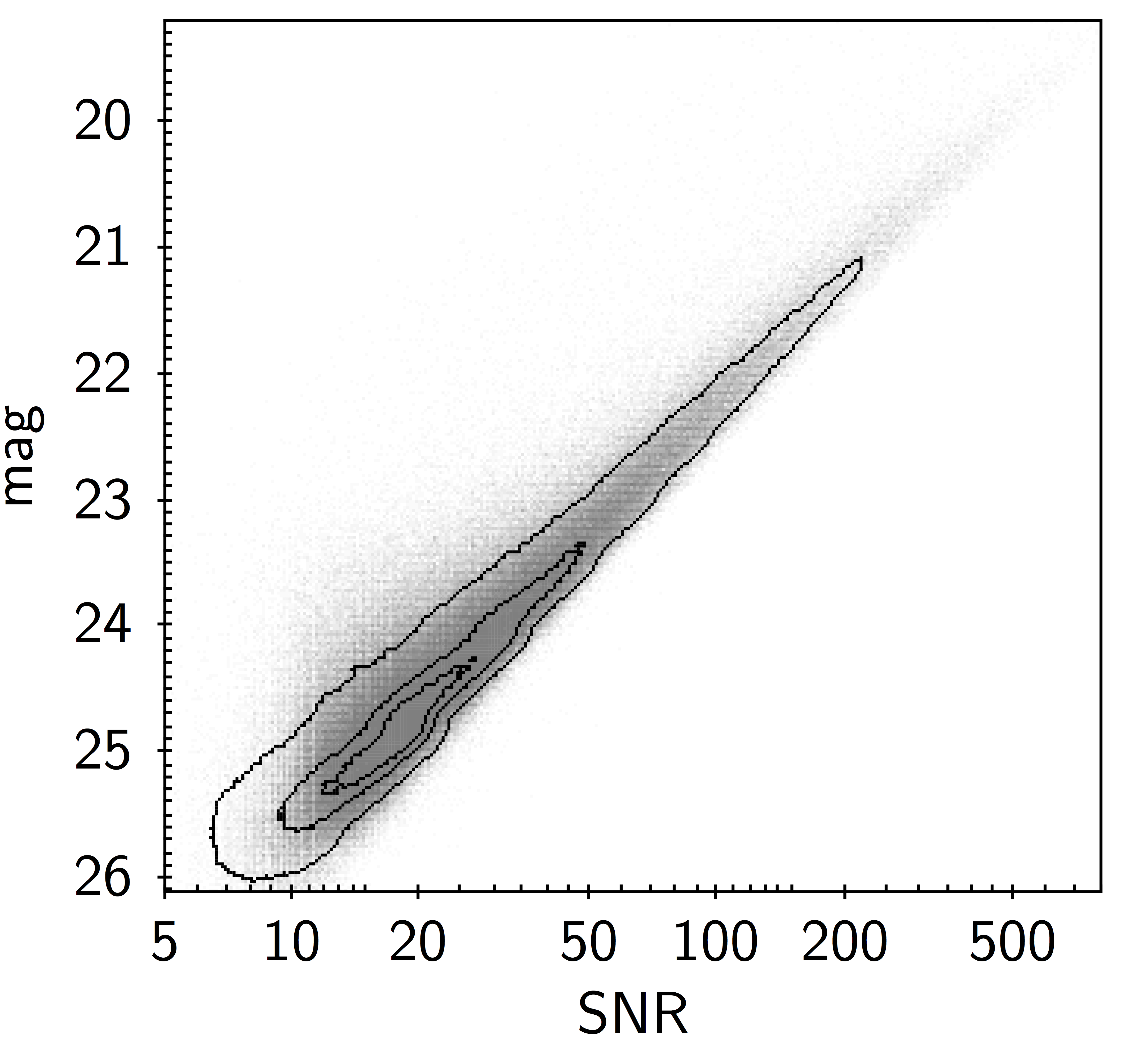
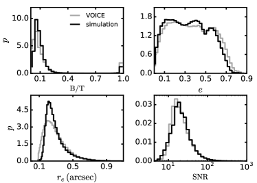
Several cuts are then applied to the shear catalogs for bias analysis. First of all, only galaxies with non-zero weight are selected. Since the properties of galaxies are analyzed as weighted average in the following sections, this cut does not affect our bias calibrations. We further reject the potentially problematic galaxies which are flagged as non-zero by LensFit. After these constraints, we match these catalogs with the mock sample described in Section 3.1 to obtain the true shear values for the galaxies. This matching is done using a $k$-d tree nearest neighbor search algorithm which is fast and efficient for large dataset. An appropriate aperture selection for the matching is essential given the existence of neighboring galaxies. A larger aperture can increase the probability of spurious matches, while too small aperture makes many faint galaxies miss out due to the noise-induced mismatch of the coordinates. It is found that an aperture radius of 0.6 arcsec, corresponding to three pixels, can efficiently remove spurious detections and reduce the probability of mismatch for neighboring galaxies. Finally, about 2.3 million galaxies are obtained in the sample for bias analysis. Figure 1 shows the two-dimensional weighted distributions of magnitudes and ellipticity versus SNR for the observation and simulation data. The double-peak distribution of ellipticity is attributed to different ellipticity priors between the disc-dominated and bulge-dominated galaxies (Miller et al., 2013).

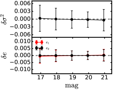
Since the dominant contribution to the shear biases results from the imperfect PSF modeling, an appropriate simulation should be capable to capture the main features of the observed PSF, especially the spatial and temporal variations. To validate the PSF model used in the simulations, we follow a similar methodology of Zuntz et al. (2017). We calculate the size and shape residuals between the stars in the observed single exposure images and the corresponding PSF modeled by PSFEx. The stars are identified by finding the stellar locus in the size-magnitude diagram with magnitude $16.0<r_{\mathrm{mag}}<22.0$ and SNR higher than 20. Compared to the stars used for PSF modeling as described in Section 3.2, we identified more fainter and lower SNR stars for testing. The size and the shape are estimated adaptively by calculating the moments of the light profile (Hirata & Seljak, 2003), encoded in the Galsim toolkit. This method can estimate the best-fit elliptical Gaussian to the star and calculate the $\sigma$ value (in unit of arcsec; defined as $|\det(M)|^{1/4}$ where $M$ is the metrix of the moments) as a representation of the size. The ellipticity is defined as $\bf{e}=(a-b)/(a+b)\exp(2\mathrm{i}\theta)$ where $a$, $b$ and $\theta$ are the major axis, the minor axis, and the orientation of the best-fit ellipse, respectively. Figure 2 compares the size and ellipticity residuals of the observed stars and the modeled PSF interpolated to the same image positions. The dots indicate the median residuals in each magnitude bin, while the uncertainties are given by Poisson errors. Within the errorbars, the size and ellipticity residuals are consistent with zero within the magnitude range, showing a good agreement between the modeled PSF used in our simulations and that of real observations.

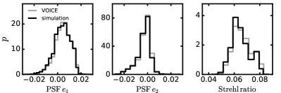
Further comparisons of the PSF parameters estimated by LensFit between the simulation and observation are shown in Figure 3. It can be seen that the weighted distributions of the two ellipticity components and the Strehl ratio parameter measured from simulated images are in good agreement with the observed data. The significant difference in distributions between the two ellipticity components implies the complicated PSF variations in the observations. One possible reason is that the long time span in observations for every tile makes the PSF pattern varied remarkably. The small survey area of VOICE may also be a reason because certain differences of $e_{1}$ and $e_{2}$ can persist. This is in contrast to surveys with a large sky coverage, for which the statistical distribution of PSF over all the fields is approximately isotropic. Our PSF models can properly reproduce the PSF features existed in VOICE observations.

In addition, Figure 4 further compares the weighted distributions of some galaxy parameters measured by LensFit from the simulation and observed data. The bulge fraction derived from simulation is well-matched with the VOICE data. The small differences of the scalelength and SNR indicate that small and faint objects are still absent in our simulation although we have reduced the stamp size in simulation according to the galaxies’ scalelength and magnitude to suppress this effect. The discrepancy presumably results partly from the different intrinsic size distributions between the simulation and real observation, and the fixing of background noise dispersions in the simulation. We can also see small differences in the ellipticity distributions. Such mismatch may indicate that the intrinsic ellipticity distribution used in the simulation is not exactly the same as that in the real observation. However, as demonstrated in the simulation of KiDS survey (Fenech Conti et al., 2017) where similar discrepancies in the distributions of size, SNR and ellipticities are presented, the resulting biases for the shear calibration are negligible. Through changing the ellipticity distributions, similar conclusion was also drawn even in the Euclid-like simulation (Hoekstra et al., 2017). We will discuss these more in Section 5.

4 Bias Calibration

Following Heymans et al. (2006), the accuracy of the reduced shear $g^{\mathrm{obs}}$ can be modeled in terms of the multiplicative bias $m$ and additive bias $c$ relating to the true shear $g^{\mathrm{true}}$ as

$$g^{\mathrm{obs}}_{i}=(1+m_{i})\times g^{\mathrm{true}}_{i}+c_{i},$$

where $g^{\mathrm{obs}}$ denotes the weighted average of the ellipticity measured by LensFit and the subscript $i$ refers to the two shear components.

The multiplicative bias and additive bias generally depend on the observed galaxy properties, such as the SNR and galaxy size. The additive bias primarily stems from the residuals in modeling the PSF anisotropy. It can be empirically corrected using the observed data. The multiplicative bias, a change of the amplitude of the shear, is mainly attributed to the background noise and pixelation, and most likely affects the shape estimate of faint galaxies. It is generally calibrated through image simulations.

In this section, we perform detailed bias calibrations for the measured galaxy shape. We note that the binning strategy for each observable adopted in this work is by equalizing the total number of galaxies in each bin. The weighted average is assigned as the center of each bin for the corresponding observable. We use the bootstrap method with 100 realizations to derive the uncertainties of the estimated shear in each bin. The $\chi^{2}$ minimization is then applied to yield the multiplicative and additive biases as well as the associated uncertainties.

4.1 Selection Bias

Besides the bias resulting from noise and model fitting, the source detection and shape measurement procedures can also introduce bias. This kind of bias is usually referred as selection bias and it was extensively discussed in many studies through image simulations (Kaiser, 2000; Bernstein & Jarvis, 2002; Hirata & Seljak, 2003; Heymans et al., 2006). Due to the difficulties in accurately measuring the shape of faint and small galaxies for many shape measurement methods, these galaxies suffer from more severe selection bias than the bright ones. Therefore, the bias is expected to be a function of the magnitude (or equivalently the SNR) and galaxy size, and can arise in both the observation and simulation. In the KiDS simulation, Fenech Conti et al. (2017) reported a significant multiplicative selection bias which was as large as 4.4% after averaging the true sheared ellipticity of galaxies with non-zero weights. It showed an obvious dependence on the magnitude and major-axis scalelength $r_{e}$. However, the dependency is reduced when we consider the geometric average of the major- and minor-axis scalelengths, denoted as $r_{ab}$, because it is less correlated with the measured ellipticity.

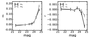
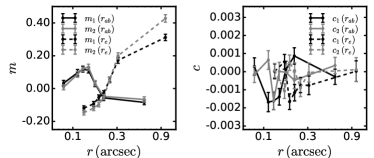
Following a similar scheme, in our simulation, we quantify the selection bias by analyzing the input sheared ellipticity of galaxies in terms of the observables. As described in Section 3, only galaxies detected in the observations are used to generate the simulated images, and we find similar number of galaxies with shape measurements compared to that of observation. For those galaxies detected in the simulated mosaic images using SExtractor, the selection bias is derived by comparing the average of the input true sheared ellipticity with true shear. In this case, the effect of noise bias vanishes, and biases stemming from the detection procedures, including the potential cancellation of zero shape noise implementation due to undetected galaxies, are dominant. It turns out that the selection bias is almost negligible at this stage. On the other hand, if considering only the galaxies with non-zero weight after running LensFit, the multiplicative selection bias becomes apparent for faint galaxies, as shown in Figure 5. The top panel of Figure 5 displays the dependence of the selection bias on magnitude. It can be seen that the multiplicative selection bias is nearly zero at magnitude brighter than 24.0 mag. It increases dramatically at fainter magnitudes because of the noise effect that results in a considerable fraction of shape measurement failure. Similar trend can also be seen for the additive bias. The multiplicative bias also exhibits a strong dependence on the major-axis scalelength $r_{e}$, as shown in the bottom panel of Figure 5. However, an apparent lower correlation is seen by adopting $r_{ab}$. The additive bias does not present significant correlations with either definition of the galaxy size. In our following analyses, we use $r_{ab}$ as the proxy of galaxy size to perform bias calibration.

As discussed above, the shear signals measured from both simulation and observation are supposed to be subjected to the selection bias. Therefore, to calibrate the shear in the VOICE survey, it is essential to take into account all the sources of bias, including the selection bias, the noise and model biases, through our simulation. In the following sections, we systematically investigate the bias calibration based on the observables SNR and $r_{ab}$ since they are the two predominant quantities that the bias depends on.

Figure 5: Top panel: the multiplicative and additive selection biases as a function of magnitude for galaxies with non-zero weight. Bottom panel: the multiplicative and additive selection biases as a function of galaxy size. The solid lines represent the size $r_{ab}$ defined as the geometric average of the major- and minor-axis scalelengths, while the dashed lines indicate the scalelength $r_{e}$ along major axis. Note that both of them are calculated through LensFit output.

4.2 Empirical Calibration

Figure 6: The multiplicative and additive biases of the measured shapes as a function of SNR (top panel) and size (bottom panel).

Figure 7: The multiplicative ($m_{+}$, $m_{\times}$) and additive ($c_{+}$, $c_{\times}$) biases of the measured shapes as a function of SNR. The bias components are derived by aligning the galaxy’s ellipticity and shear to the corresponding PSF ellipticity.

Figure 8: Top panel: Multiplicative bias distributions ($m_{1}$ on the left and $m_{2}$ on the right) in the SNR – $r_{ab}$ two-dimensional plane. For clarity, a “lanczos” kernel is applied to smooth the discrete values. Bottom panel: Estimated error distributions of the multiplicative biases.

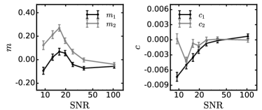
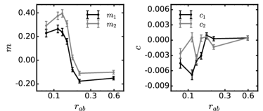
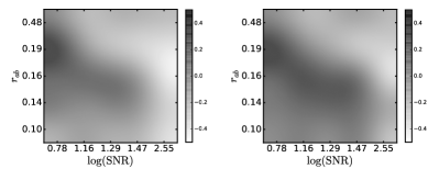
The biases of the shear measured from the simulation as a function of galaxy SNR and size are shown in Figure 6. As expected, both the multiplicative bias and additive bias get larger for galaxies with low SNR and small size. The maximum of the absolute values reaches 0.4 for multiplicative bias and 0.008 for additive bias. One feature shown in Figure 6 is that the two components for both multiplicative and additive biases present somewhat different amplitudes. As discussed in Massey et al. (2007) and Mandelbaum et al. (2015), the additive bias components in the pixel coordinate frame probably result from the selection bias and potential numerical artifacts. The difference between the two multiplicative components $m_{1}$ and $m_{2}$ may be due to the effect of pixelization of the galaxy images and PSF profiles. In order to check the hypothesis, we compute the tangential and cross components of the shape and shear for each galaxy in a reference system aligned with the PSF ellipticity axes. The derived bias components are defined as ($m_{+}$, $c_{+}$) and ($m_{\times}$, $c_{\times}$), respectively. Since the PSF ellipticity is approximately randomly orientated with respect to the pixel axes, the difference due to pixelization is expected to be cancelled out. As illustrated in Figure 7, the $m_{+}$ and $m_{\times}$ have much more similar amplitudes than that of $m_{1}$ and $m_{2}$. The small residual difference might be related to the somewhat different distributions of the two PSF components shown in Figure 3. The PSF anisotropy explains the difference of $c_{+}$ and $c_{\times}$. To simplify the shear analysis, in the following we will focus on the shear calibration in the original pixel frame.

Because of the amplitude differences for the two components, we cannot adopt a uniform analytical expression, such as the function used in Miller et al. (2013), to describe the calibration parameters. We therefore take the similar approach applied in KiDS simulation (Fenech Conti et al., 2017) to use the bin-matching method on the SNR – $r_{ab}$ surface to calibrate the bias. Specifically, we firstly bin the galaxies by SNR and size $r_{ab}$ in the two-dimensional plane, and then derive a constant bias in each bin. If one observed galaxy falls into a certain bin, its ellipticity will be calibrated by applying the corresponding biases.

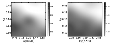
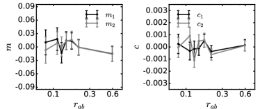
Due to our limited sky coverage and relatively small amount of galaxies, an appropriate binning scheme is crucial to derive valid bias calibration results. If the number of bins is too small, we may miss out on some real features in the bias surface. However, the statistical uncertainty arises if there are too many bins, and that can result in extra artificial bias. For our simulation, we find that a five-bin scheme along both SNR and $r_{ab}$ axis can yield robust calibration. In this case, the average error of the multiplicative bias in each bin is 0.04, while the SNR_m (defined as $m/m_{err}$, where $m_{err}$ is the estimated error of $m$) is close to 4.8. The top panel of Figure 8 illustrates the two-dimensional distributions of the two multiplicative bias components in the SNR – $r_{ab}$ plane. It is seen that while they present similar dependence on the two observables, the amplitudes of $m_{2}$ are systematically larger. The distributions of corresponding error $m_{err}$ are shown in the bottom panel. As expected, galaxies with smaller size and lower SNR suffer more significant calibration uncertainties. Figure 9 shows the final residuals after bias calibration. It can be seen that the multiplicative bias is well within 0.03 over the entire SNR and size ranges, and the additive bias almost vanishes. The residuals do not present strong dependence on the SNR and galaxy size. Overall, both the residual multiplicative bias and additive bias are consistent with zero, indicating that the calibration is unbiased.

Figure 9: The residual multiplicative and additive biases after calibration using the bin-matching method as a function of measured SNR (top panel) and size (bottom panel).

5 Calibration Sensitivity

As we have discussed in Section 3, the sample extracted from simulation misses some faint and small size galaxies. The distributions of the ellipticity between the simulation and observation are also slightly different. These differences may result in extra residual bias when applying the calibration results to observation. Hoekstra et al. (2017) studied the sensitivities to these effects based on Euclid-like image simulation, and concluded that the multiplicative bias is indeed affected by these factors. However, they demonstrated that the amplitude change of the multiplicative bias is always less than 0.005 by varying the corresponding distributions. Similar conclusions were also drawn in the KiDS simulation (Fenech Conti et al., 2017), which stated that the sensitivities of the multiplicative bias to the different distributions can be safely neglected for the present accuracy requirement ($m\sim 0.01$) in weak lensing surveys. VOICE and KiDS surveys share the same instrument and observational configuration. The VOICE survey is deeper, but the area is much smaller than that of KiDS. Thus the number of galaxies with successful shear measurements is smaller, resulting in larger statistical uncertainties in cosmological analyses. We therefore expect that the effect of lacking of small and faint galaxies in our simulation on the shear bias calibration is even less significant than that of KiDS. However, for future deep and wide surveys, this can be an issue (Hoekstra et al., 2017).

On the other hand, since the galaxies in our simulation are only from observation without including those below detection limit, the undetected galaxies may introduce potential bias. In addition, since the positions of galaxies in the simulated images exactly match those of real galaxies, it is possible to study the impact of the galaxy blending effect on the multiplicative bias. We focus on the sensitivity analyses of these two factors in this section.

5.1 Impact of Galaxies Below Detection Limit

Figure 10: Magnitude distributions of different $r$-band photometric catalogs with errorbar estimated by the Poisson statistics. The magnitudes are from UVUDF F606W band (blue), GEMS F606W band (light blue), COSMOS2015 $r$ band (cyan) and VOICE $r$ band (black), respectively. The red solid line represents the best fit for VOICE $20.0<m_{r}<24.0$, GEMS $24.0<m_{r}<26.0$ and UVUDF $26.0<m_{r}<28.0$ data.

Figure 11: Residual multiplicative bias $\delta{m}$ due to the presence of undetected galaxies as a function of SNR.

For objects fainter than the limiting depth, Hoekstra et al. (2015) found that they make the multiplicative bias of brighter galaxies underestimated in the cluster environment because they are likely to be blenders or skew the background noise. Hoekstra et al. (2017) further analyzed the issue, and found that the multiplicative bias is affected by both the size distribution and count slope of the undetected galaxies. Fenech Conti et al. (2017) also discussed the effect in KiDS simulation and found a negligible bias compared to the survey statistical uncertainties.

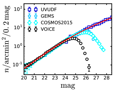
To mimic the realistic magnitude distribution of the undetected galaxies in VOICE observation, photometric measurements from other deeper imaging are included, which are HST/ACS $F606W$-band data from UVUDF (Rafelski et al., 2015) and GEMS (Rix et al., 2004; Griffith et al., 2012), Subaru/SuprimeCam $r$-band data from COSMOS2015 catalog (Laigle et al., 2016). These filters are analogous to the OmegaCam $r$ filter. Figure 10 shows their number density distributions of galaxies as a function of magnitude $m$. It can be seen that they are consistent for magnitude brighter than 25.0 mag. A second order polynomial is adopted to fit the distribution using VOICE counts between $20.0<m_{r}<24.0$, GEMS counts between $24.0<m_{r}<26.0$ and UVUDF counts between $26.0<m_{r}<28.0$. The least-square result is

$$\log(n)=-15.012+0.947m_{r}-0.013m_{r}^{2},$$

where $n$ is the number of galaxies per square arcminute in a given magnitude bin with width of 0.2 mag. In our simulation, we truncate the magnitude of undetected galaxies to 28.0 mag, and restrict their bright-end to 25.0 mag which is approximately equal to the maximal value in the distribution of VOICE catalog, as depicted in Figure 10. Consequently, the total number density of these undetected galaxies is as many as 185 per square arcminute.

Unlike the simulation of the detected galaxies as described in Section 3, the celestial positions of the undetected galaxies are randomly assigned. The size and intrinsic ellipticity are drawn from the same prior distributions as stated in Miller et al. (2013). Since these galaxies are below the noise level even in the stacked image, extra shear components are not expected to contribute significant systematics. Therefore, null shear is assigned to these galaxies. Furthermore, to save simulation time, we do not generate the undetected galaxy images chip by chip as for the procedure for the detectable ones. Instead, we sprinkle them to a noiseless image mosaic centered at the same celestial position as that of the CDFS field. The PSF model is assumed to be Gaussian with constant FWHM fixed to the median value of the observation. Finally, for a given CCD chip (or sky coverage), we extract the corresponding sub-image from this image mosaic, and then add it to the previously simulated image.

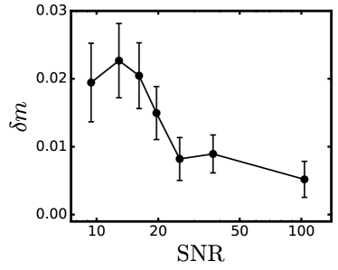
We follow the same steps as presented in previous sections to perform shear measurements and bias analyses for the detected galaxies using the new set of images. Compared to the results derived from no-faint-galaxies simulation, the multiplicative bias of the entire sample increases only by 0.003, while the additive bias shows negligible change. Figure 11 shows the residual multiplicative bias $\delta{m}$ as a function of SNR. Here $\delta{m}$ is defined as $[(\delta{m_{1}})^{2}+(\delta{m_{2}})^{2}]^{1/2}$, where $\delta{m_{i}}$ represents the difference of multiplicative biases between the two sets of simulation. Overall, our result indicates that galaxies with lower SNR (or fainter magnitude) suffer more from the undetected galaxies. Since the amplitude is well below the residual bias we achieve in Section 4, we claim that the sensitivity of the multiplicative bias to the undetected galaxies for our simulation is insignificant. However, as illustrated in Figure 11 the impact of undetected galaxies has to be taken into account for more accurate shear measurements as required by future large and deep surveys, especially for galaxies with low SNRs.

Figure 12: The multiplicative bias as a function of SNR. The black and grey dashed lines represent the two bias components $m_{1}$ and $m_{2}$ derived from the entire simulation sample, while the solid lines are the corresponding components after rejecting the neighboring galaxies. The dotted lines indicate the average bias derived from the subsamples of galaxies by repeated sampling 100 times.

Table 2: The ellipticity dispersions of the neighboring galaxies in the four fields. Column 1 represents the maximum distance between any galaxy pair. The number of galaxies with non-zero weight and zero flag is shown in Column 2, while Column 3 indicates the fraction relative to the neighboring galaxies without any cut. Column 4&5 are the dispersions of the two ellipticity components.

$r$	$n_{\mathrm{gal}}$	fracion	$\sigma_{e_{1}}$	$\sigma_{e_{2}}$
1.0″	124	33.6%	0.403	0.421
2.0″	1858	7.8%	0.333	0.350
3.0″	25746	31.6%	0.307	0.309

Figure 13: Examples of four very close neighbors in CDFS1/GEMS field. The top panel shows galaxies observed in GEMS survey, while the corresponding stacked images from the VOICE survey are displayed in bottom panel. The size of each stamp is $5\arcsec\times 5\arcsec$, centered on the target galaxy in VOICE image.

5.2 Impact of Blending Galaxies

As discussed above, the simulation strategy in this work enables us to study the effect of the neighboring galaxies on the measured shear. These galaxies can be either physically related neighbors with similar shear or projected close pairs but with different redshifts and shape distortions. Although LensFit has encoded an algorithm to deal with them (Miller et al., 2013), potential bias is still inevitable in the measured shear due to the inappropriate modeling of the surface brightness distributions in the overlapped regions. In this section, we mainly concentrate on their contribution to the multiplicative bias.

First of all, we compare the ellipticity dispersions of the real galaxies in the parent sample which is constructed from observation and used as simulation input (see Sec 3.1). As shown in Table 2, the dispersion increases as the neighbors get closer to each other, and is always larger than that of all galaxies in the parent sample. We note that a large fraction of the neighbors with separation less than $1.0\arcsec$ have non-zero weight. Careful analysis shows that LensFit regards most of these close galaxy pairs as single and extended galaxies. The resulted ellipticity dispersion is almost 38.0% larger than that of the parent sample. Clearly, these galaxies should be excluded from further shear analyses. For galaxy pairs with the separation less than $r=3.0\arcsec$, about 31.6% of them have shape measurements with non-zero weight. Their number density is about 1.3 per square arcmin, and the ellipticity dispersion is about 3.4% larger than that of the full shear sample. Rejecting these galaxies results in a $\sim$8.2% decrease of the effective number density of galaxies. On the other hand, because of relatively large statistical uncertainties of VOICE data, the results of cosmic shear two-point correlations have negligible changes if these galaxies are excluded.

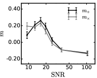
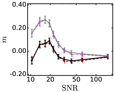
We further quantify their impact on the multiplicative bias using the simulated shear catalogs. Considering different sizes of galaxies, to reflect better the blending effect, we redefine galaxy neighbors using an adaptive scheme with a separation less than four times of the sum of their major axis scalelengths. Under this definition, the fraction of neighbors with shape measurements is about 6%. A clean sample is then constructed by rejecting these neighbors from the full simulation sample. The solid lines in Figure 12 show the two multiplicative bias components, derived from the clean sample, as a function of SNR. For comparison, the bias components from the full sample are illustrated as dashed lines. It is seen that the multiplicative biases of the two components become systematically smaller for the clean sample than those of the full sample, although the differences are not very considerable. It is interesting to note that the differences are larger for galaxies with high SNR. This is because the SNRs of the neighboring galaxies are systematically overestimated, and their effect on the bias is therefore more significant at high SNRs. We find that their median SNR is 33.0, comparing to 24.2 of the full sample.

The clean sample contains slightly less galaxies. To see if the number change can affect the bias calibration, we randomly select an equal number of galaxies as the clean sample from the full simulation sample, and estimate the multiplicative bias. The sampling procedure is repeated by one hundred times. The dotted lines in Figure 12 show the average of the bias as a function of SNR. We see that the results are basically the same as those of the full sample, showing that the blending effect does contribute to the differences between the clean and the full sample. The differences are at the level of $0.002$.

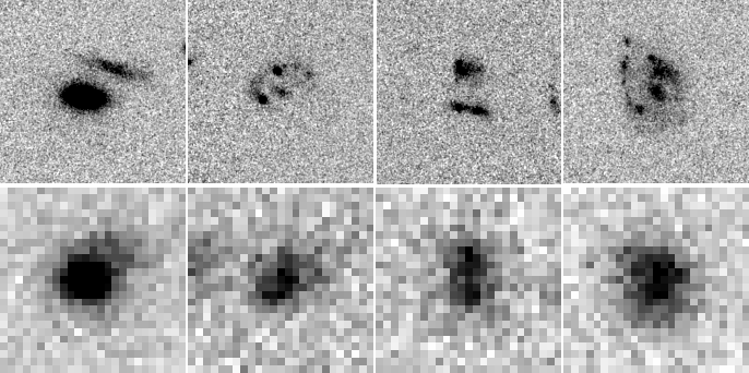
Besides the neighbors that can be unambiguously identified, there are pairs that are so close and misidentified as single objects. This is particularly the case for ground-base observations. To check this for the VOICE sample, we use the data of Galaxy Evolution From Morphology And SEDs (GEMS; Rix et al. (2004)) observed using Hubble space telescope. The overlapped area between VOICE and GEMS is about 800 arcmin². We identified 2185 such blenders down to magnitude of 26.0 mag in our parent sample by following the similar method in Dawson et al. (2016). This accounts for about 5.0% of the total number of galaxies in the overlapped area. We find that 68% of them have shape measurements with dispersion of 0.33 for the two ellipticity components. Their weighted number density is 0.92 per arcmin². Figure 13 exhibits four typical examples of these blenders. Apparently, they are observed as multiple objects in the GEMS survey, and show diverse morphologies. However, in the VOICE observations, they are identified as single galaxies. Their shear measurements using VOICE data cannot be correct, and thus should be excluded. We do not expect that they affect significantly our VOICE shear analyses because of the large statistical errors. For the upcoming deep and wide ground-based surveys, however, we do need to consider such blenders, and quantify carefully how they affect the weak lensing cosmological studies.

In summary, galaxies fainter than the detection limit and the blending effect from neighboring galaxies contribute to the multiplicative bias at the level of less than $\sim$0.5%. The small differences between our simulation catalog and the observed data do not induce noticeable biases (less than $1\%$) considering the statistical uncertainties of the VOICE shear sample. Our final multiplicative shear calibration residual is $\sim$3%, which reflects mainly the statistical errors.

6 Summary

The VOICE survey has observed $\sim$ 4  deg² in the CDFS field in $ugri$ optical bands using VST/OmegaCam. After a cut in FWHM $<$ 0.9 arcsec, the survey consists of more than a hundred exposures for each tile, and the depth is about 1.2 magnitude deeper than that of KiDS survey. We have performed shear measurements, and obtained an effective number density of galaxies $n_{g}\sim 16.35\hbox{ arcmin}^{-2}$. In the work, we perform detailed shear bias calibrations for the VOICE survey based on $r$-band image simulations. Many observational conditions, such as the dithering pattern, background noise, celestial positions and brightness of the detected objects, have been taken into account in the simulations in order to mimic the real observations. The PSFEx package is used to model the spatially varied PSF in every exposure. The simulated single exposure images are generated by the Galsim toolkit, and the galaxy shapes are measured by LensFit, a Bayesian fitting code that has been extensively applied to many other large surveys, such as CFHTLenS, KiDS and RCSLenS. Overall, our simulations present good agreements with the characteristics of observations, especially the distributions of the PSF parameters. We notice that some small and faint galaxies are missing in our simulations comparing to the real observations. We argue that they should not affect our shear calibration significantly given the relatively low total number of galaxies in the VOICE survey. We apply the bin-matching method to the SNR and size surface to calibrate the bias of the simulation data. The final residual multiplicative bias can reach to an accuracy of 0.03 with negligible additive bias in different SNR and size bins. The average residual bias of the full sample is consistent with zero.

Our studies demonstrate the applicability of Lensfit for shear measurements to data with more than a hundred exposures. The image simulation analyses show that the change of the deblending threshold from the fiducial $2\sigma$ to $5\sigma$ does not introduce considerable issues.

We further discuss the sensitivity of the bias calibration to the undetected and blending objects. The undetected objects are likely to skew the background noise so that they can potentially bias the shape measurements of galaxies, especially those with low SNR. Taking the depth and noise level, and the relatively large statistical uncertainties into account, we find that the impact of the undetected galaxies is negligible for the VOICE survey. Additionally, we highlight the bias resulting from galaxy blending effect. Although a large fraction of neighboring galaxies has been excluded by LensFit, there are still 31.6% of neighboring galaxies with separation less than $3\arcsec$ having shape measurements. The ellipticity dispersion of them is 3.4% larger than the average value of the parent sample, and the weighted number density is as large as 1.3 per square arcmin. Considering galaxy pairs with an adaptive separation less that four times of the sum of their major axes, we find that $\sim$6% of them have shear measurements, and they contribute to additional $\sim$0.2% multiplicative bias. With the increase of depth and sensitivity, many weak lensing surveys, such as HSC and LSST, aiming to achieve much more accurate weak lensing studies than that of VOICE, have to deal with the blending effect more carefully.

References

- Abbott et al. (2016) Abbott, T., Abdalla, F. B., Allam, S., et al. 2016, Phys. Rev. D, 94, 022001
- Bartelmann & Maturi (2017) Bartelmann, M., & Maturi, M. 2017, Scholarpedia, 12, 32440
- Becker et al. (2016) Becker, M. R., Troxel, M. A., MacCrann, N., et al. 2016, Phys. Rev. D, 94, 022002
- Benjamin et al. (2007) Benjamin, J., Heymans, C., Semboloni, E., et al. 2007, MNRAS, 381, 702
- Bernstein & Jarvis (2002) Bernstein, G. M., & Jarvis, M. 2002, AJ, 123, 583
- Bertin & Arnouts (1996) Bertin, E., & Arnouts, S. 1996, A&AS, 117, 393
- Bertin (2011) Bertin, E. 2011, Astronomical Data Analysis Software and Systems XX, 442, 435
- Bosch et al. (2018) Bosch, J., Armstrong, R., Bickerton, S., et al. 2018, PASJ, 70, S5
- Botticella et al. (2017) Botticella, M. T., Cappellaro, E., Greggio, L., et al. 2017, A&A, 598, A50
- Bridle et al. (2009) Bridle, S., Shawe-Taylor, J., Amara, A., et al. 2009, Annals of Applied Statistics, 3, 6
- Cappellaro et al. (2015) Cappellaro, E., Botticella, M. T., Pignata, G., et al. 2015, A&A, 584, A62
- Chang et al. (2013) Chang, C., Jarvis, M., Jain, B., et al. 2013, MNRAS, 434, 2121
- Dawson et al. (2016) Dawson, W. A., Schneider, M. D., Tyson, J. A., & Jee, M. J. 2016, ApJ, 816, 11
- de Jong et al. (2015) de Jong, J. T. A., Verdoes Kleijn, G. A., Boxhoorn, D. R., et al. 2015, A&A, 582, A62
- Falocco et al. (2015) Falocco, S., Paolillo, M., Covone, G., et al. 2015, A&A, 579, A115
- Fenech Conti et al. (2017) Fenech Conti, I., Herbonnet, R., Hoekstra, H., et al. 2017, MNRAS, 467, 1627
- Fu & Fan (2014) Fu, L.-P., & Fan, Z.-H. 2014, Research in Astronomy and Astrophysics, 14, 1061-1120
- Fu et al. (2018) Fu, L., Liu, D., Radovich, M., et al. 2018, arXiv:1802.10282
- Gaia Collaboration et al. (2016) Gaia Collaboration, Brown, A. G. A., Vallenari, A., et al. 2016, A&A, 595, A2
- Giacconi et al. (2001) Giacconi, R., Rosati, P., Tozzi, P., et al. 2001, ApJ, 551, 624
- Grado et al. (2012) Grado, A., Capaccioli, M., Limatola, L., & Getman, F. 2012, Memorie della Societa Astronomica Italiana Supplementi, 19, 362
- Green et al. (2012) Green, J., Schechter, P., Baltay, C., et al. 2012, arXiv:1208.4012
- Griffith et al. (2012) Griffith, R. L., Cooper, M. C., Newman, J. A., et al. 2012, ApJS, 200, 9
- Heymans et al. (2006) Heymans, C., Van Waerbeke, L., Bacon, D., et al. 2006, MNRAS, 368, 1323
- Heymans et al. (2012) Heymans, C., Van Waerbeke, L., Miller, L., et al. 2012, MNRAS, 427, 146
- Heymans et al. (2013) Heymans, C., Grocutt, E., Heavens, A., et al. 2013, MNRAS, 432, 2433
- Hildebrandt et al. (2016) Hildebrandt, H., Choi, A., Heymans, C., et al. 2016, MNRAS, 463, 635
- Hildebrandt et al. (2017) Hildebrandt, H., Viola, M., Heymans, C., et al. 2017, MNRAS, 465, 1454
- Hirata & Seljak (2003) Hirata, C., & Seljak, U. 2003, MNRAS, 343, 459
- Hoekstra et al. (2015) Hoekstra, H., Herbonnet, R., Muzzin, A., et al. 2015, MNRAS, 449, 685
- Hoekstra et al. (2017) Hoekstra, H., Viola, M., & Herbonnet, R. 2017, MNRAS, 468, 3295
- Jarvis et al. (2016) Jarvis, M., Sheldon, E., Zuntz, J., et al. 2016, MNRAS, 460, 2245
- Kaiser (2000) Kaiser, N. 2000, ApJ, 537, 555
- Kilbinger et al. (2013) Kilbinger, M., Fu, L., Heymans, C., et al. 2013, MNRAS, 430, 2200
- Kilbinger (2015) Kilbinger, M. 2015, Reports on Progress in Physics, 78, 086901
- Kitching et al. (2008) Kitching, T. D., Miller, L., Heymans, C. E., van Waerbeke, L., & Heavens, A. F. 2008, MNRAS, 390, 149
- Kitching et al. (2012) Kitching, T. D., Balan, S. T., Bridle, S., et al. 2012, MNRAS, 423, 3163
- Kron (1980) Kron, R. G. 1980, ApJS, 43, 305
- Kuijken et al. (2015) Kuijken, K., Heymans, C., Hildebrandt, H., et al. 2015, MNRAS, 454, 3500
- Laigle et al. (2016) Laigle, C., McCracken, H. J., Ilbert, O., et al. 2016, ApJS, 224, 24
- Laureijs et al. (2011) Laureijs, R., Amiaux, J., Arduini, S., et al. 2011, arXiv:1110.3193
- Liu et al. (2016) Liu, X., Li, B., Zhao, G.-B., et al. 2016, Physical Review Letters, 117, 051101
- LSST Science Collaboration et al. (2009) LSST Science Collaboration, Abell, P. A., Allison, J., et al. 2009, arXiv:0912.0201
- Mandelbaum et al. (2014) Mandelbaum, R., Rowe, B., Bosch, J., et al. 2014, ApJS, 212, 5
- Mandelbaum et al. (2015) Mandelbaum, R., Rowe, B., Armstrong, R., et al. 2015, MNRAS, 450, 2963
- Mandelbaum (2017a) Mandelbaum, R. 2017a, arXiv:1710.03235
- Mandelbaum et al. (2017b) Mandelbaum, R., Lanusse, F., Leauthaud, A., et al. 2017b, arXiv:1710.00885
- Mandelbaum et al. (2018) Mandelbaum, R., Miyatake, H., Hamana, T., et al. 2018, PASJ, 70, S25
- Massey et al. (2007) Massey, R., Heymans, C., Bergé, J., et al. 2007, MNRAS, 376, 13
- Miller et al. (2007) Miller, L., Kitching, T. D., Heymans, C., Heavens, A. F., & van Waerbeke, L. 2007, MNRAS, 382, 315
- Miller et al. (2013) Miller, L., Heymans, C., Kitching, T. D., et al. 2013, MNRAS, 429, 2858
- Miyazaki et al. (2012) Miyazaki, S., Komiyama, Y., Nakaya, H., et al. 2012, Proc. SPIE, 8446, 84460Z
- Oke & Gunn (1983) Oke, J. B., & Gunn, J. E. 1983, ApJ, 266, 713
- Oliver et al. (2000) Oliver, S., Rowan-Robinson, M., Alexander, D. M., et al. 2000, MNRAS, 316, 749
- Rafelski et al. (2015) Rafelski, M., Teplitz, H. I., Gardner, J. P., et al. 2015, AJ, 150, 31
- Rix et al. (2004) Rix, H.-W., Barden, M., Beckwith, S. V. W., et al. 2004, ApJS, 152, 163
- Rowan-Robinson et al. (2004) Rowan-Robinson, M., Lari, C., Perez-Fournon, I., et al. 2004, MNRAS, 351, 1290
- Rowe et al. (2015) Rowe, B. T. P., Jarvis, M., Mandelbaum, R., et al. 2015, Astronomy and Computing, 10, 121
- Samuroff et al. (2018) Samuroff, S., Bridle, S. L., Zuntz, J., et al. 2018, MNRAS, 475, 4524
- Tozzi et al. (2001) Tozzi, P., Rosati, P., Nonino, M., et al. 2001, ApJ, 562, 42
- Vaccari (2015) Vaccari 2015, Proceedings of ”The many facets of extragalactic radio surveys: towards new scientific challenges” Conference, 20-23 October 2015, Bologna, Italy, Proceedings of Science, 267, 27
- Vaccari (2016a) Vaccari 2016a, Proceedings of ”The Universe of Digital Sky Surveys” Conference, 25-28 November 2014, Naples, Italy, Astrophysics and Space Science Proceedings, 42, 71
- Vaccari et al. (2016b) Vaccari et al. 2016b, Proceedings of the 4th Annual Conference on High Energy Astrophysics in Southern Africa, 25-26 August 2016, Cape Town, South Africa, Proceedings of Science, 275, 26
- Viola et al. (2014) Viola, M., Kitching, T. D., & Joachimi, B. 2014, MNRAS, 439, 1909
- Zuntz et al. (2017) Zuntz, J., Sheldon, E., Samuroff, S., et al. 2017, arXiv:1708.01533