Generalizing parallel replica dynamics: trajectory fragments, asynchronous computing, and PDMPs

Abstract

We study the Parallel Replica Dynamics in a general setting. We introduce a trajectory fragment framework that can be used to design and prove consistency of Parallel Replica algorithms for generic Markov processes. We use our framework to formulate a novel condition that guarantees an asynchronous algorithm is consistent. Exploiting this condition and our trajectory fragment framework, we present new synchronous and asynchronous Parallel Replica algorithms for piecewise deterministic Markov processes.

65C05, 65C20, 65C40, 65Y05, 82C80

1 Introduction

Many problems in applied sciences require the sampling of complex probability distributions. In computational chemistry – which is the main setting of this article – such distributions can arise from stochastic models of molecular dynamics [34] or chemical reaction networks [2], while obstacles to efficient sampling include high dimensionality and metastability, the latter being the tendency to become stuck in certain subsets of state space [31]. Some attempts to surmount these difficulties have been based on importance sampling and stratification [51, 57, 58, 60], interacting particles [17, 18, 19, 20], coarse graining and preconditioning [4, 35, 56], accelerated dynamics [32, 53, 61, 62] and nonreversibility [21, 25, 33, 48, 68].

This article concerns the Parallel Replica Dynamics (ParRep) [62], an accelerated dynamics method designed to overcome metastability. ParRep has two distinct advantages over many other enhanced sampling methods. First, it computes correct dynamical [5, 30, 61] as well as stationary or equilibrium [3, 65] quantities associated with a stochastic process. And second, ParRep is very general: it only requires mild assumptions on the underlying process. Indeed, though originally intended for Langevin dynamics [30, 61, 63], straightforward extensions of ParRep to discrete and continuous time Markov chains have appeared in [3, 5, 65].

The goal of this article is as follows. First, we introduce a new mathematical framework that may be used to design, and prove consistency of, ParRep algorithms for Markov processes satisfying a few mild assumptions. Second, we use our framework to obtain valuable insights about asynchronous computing. In particular, we present specific, novel conditions that ensure an asynchronous ParRep algorithm is consistent. Lastly, we construct ParRep algorithms for piecewise deterministic Markov processes (PDMPs) in both the synchronous and asynchronous setting, leaning on our new framework to demonstrate their consistency. Asynchronous ParRep algorithms must be carefully designed, since as we show below, inaccuracies can arise when the speed of computing paths of the underlying process is coupled to the process itself.

PDMPs are emerging as an useful tool in fields as diverse as applied probability [38], computational chemistry [1, 7, 26, 28, 37, 44, 49, 50, 66], machine learning [9, 45, 67], and big data [6]. As indicated by the name, PDMPs move along deterministic paths in between random jump times. In the context of chemical reaction networks, PDMPs called hybrid models can be obtained by approximating fast reactions by a deterministic flow, and representing slow reactions with an appropriate Poisson process [28, 66]. The resulting PDMPs can be metastable [10, 11, 12, 13, 39, 40, 41, 42, 43], making direct simulation unattractive. Several PDMP-based algorithms have also been proposed for sampling from distributions known up to normalization – like the Boltzmann distribution or the posterior distribution in Bayesian analysis – including Event chain Monte Carlo [26, 37], the Zig-Zag process [6], and the Bouncy Particle Sampler [9, 38]. Below, we give a general argument suggesting these PDMPs also become metastable under certain conditions.

This article is organized as follows. Section 2 defines notation that we use throughout. In Section 3, we formally define metastability in terms of quasistationary distributions. We describe ParRep in more detail, and explain what we mean by a consistent ParRep algorithm, in Section 4. In Section 5 we outline a general mathematical framework for ParRep, and in Section 6 we study synchronous and asynchronous computing. Section 7 serves as a brief introduction to PDMPs, while Section 8 outlines several ParRep algorithms for PDMPs that are based on our framework from Section 5. A numerical example is in Section 9. All proofs are in Section 10.

2 Notation

Throughout, $X(t)_{t\geq 0}$ is a time homogeneous Markov process, either discrete or continuous in time, with values in a standard Borel state space; $U$ is a subset of state space; and $g$ is a real-valued function defined on state space. Without explicit mention we assume all sets are measurable and all functions are bounded and measurable. We write $X(t)$ to refer to the process $X(t)_{t\geq 0}$ at time $t$. We denote various expectations and probabilities by ${\mathbb{E}}$ and ${\mathbb{P}}$, with the precise meaning being clear from context. We write ${\mathcal{L}}$ for the probability law of a random object, with ${\mathcal{L}}$ above an equals sign indicating equality in law. We say a random object is a copy of another random object if it has the same law as that object. When we say a collection of random objects is independent we mean these objects are mutually independent unless otherwise specified. We define $a\wedge b=\min\{a,b\}$ and $a\vee b=\max\{a,b\}$, and write $\lfloor s\rfloor$ for the greatest integer less than or equal to $s$.

3 Metastability

Informally, $U$ is a metastable set for $X(t)_{t\geq 0}$ if $X(t)_{t\geq 0}$ tends to reach a local equilibrium in $U$ much faster than it escapes from $U$. Local equilibrium can be understood in terms of quasistationary distributions (QSDs):

Definition 3.1.

Fix a subset $U$ of state space, and consider

$$T=\inf\{t\geq 0:X(t)\notin U\},$$

the first time $X(t)_{t\geq 0}$ escapes $U$. A QSD $\rho$ of $X(t)_{t\geq 0}$ in $U$ satisfies $\rho(U)=1$ and

(1) $$\rho(A)={\mathbb{P}}(X(t)\in A|{\mathcal{L}}(X(0))=\rho,\,T>t)$$

for every $t\geq 0$ and $A\subseteq U$.

Note that $\rho$ is supported in $U$. Equation (1) states that if $X(0)$ is distributed as $\rho$ and $X(t)_{t\geq 0}$ does not escape from $U$ by time $t$, then $X(t)$ is distributed as $\rho$. Throughout, we will assume the QSD of $X(t)_{t\geq 0}$ in $U$ exists, is unique, and is the long time distribution of $X(t)$ conditioned to never escape $U$. That is, we assume that for any initial distribution of $X(0)$ supported in $U$,

(2) $$\rho(A)=\lim_{t\to\infty}{\mathbb{P}}(X(t)\in A|X(s)\in U\text{ for }s\in[0,t])\quad\forall\,A\subseteq U.$$

The QSD $\rho$ can then be sampled as follows: choose a time $T_{corr}^{\rho}(U)$ for relaxation to $\rho$. Start $X(t)_{t\geq 0}$ in $U$, and if it escapes from $U$ before time $t=T_{corr}^{\rho}(U)$, restart it in $U$. Repeat this until a trajectory of $X(t)_{t\geq 0}$ remains in $U$ for a consecutive time interval of length $T_{corr}^{\rho}(U)$. This trajectory’s terminal position is then a sample of $\rho$. For more details on the QSD see for instance [16]. For conditions ensuring existence of and convergence to the QSD for general Markov processes, see [14, 15, 16].

A more formal definition of metastability is: a set $U$ is metastable for $X(t)_{t\geq 0}$ if the time scale to reach $\rho$ is small compared to the mean time to escape from $U$ starting at $\rho$. In some cases these times can be written in terms of the eigenvalues of the adjoint, $L^{*}$, of the generator $L$ of $X(t)_{t\geq 0}$, with absorbing boundary conditions on the complement of $U$. See [30] and [65] for the corresponding spectral analysis for overdamped Langevin dynamics and finite state space discrete and continuous time Markov chains, and [8] for an application of these ideas to choosing $T_{corr}^{\rho}(U)$.

4 Parallel replica dynamics

ParRep can boost the efficiency of simulating metastable processes [3, 5, 30, 62, 63, 65]. Currently, implementations have been proposed only for Langevin or overdamped Langevin dynamics [30] and discrete or continuous time Markov chains [3, 5, 65]. However, the generality of ParRep allows for extensions to any metastable time homogeneous strong Markov process with càdlàg paths, in cases where the QSD exists and metastable sets can be identified. We make this precise in the next section.

ParRep algorithms are based on two basic steps:

• A step in which $X(t)_{t\geq 0}$ is allowed to reach the QSD in some metastable set $U$, using direct or serial simulation – called the decorrelation step;

• A step generating an escape event from $U$, starting from the QSD, using parallel simulation – called the parallel step.

By escape event we mean the random pair $(T,X(T))$, where $T$ is the time for $X(t)_{t\geq 0}$ to escape from $U$ when $X(0)$ is distributed as the QSD in $U$, and $X(T)$ is the corresponding escape point. The parallel step efficiently computes an escape event starting from the QSD via a sort of time parallelization.

The decorrelation step, as it uses only serial simulation, is exact. By exact we mean there is zero error – except for the inevitable error in simulating $X(t)_{t\geq 0}$ arising from numerical discretizations, which we will ignore. Our analysis will therefore focus on the parallel step.

The parallel step is sometimes divided into two subrouties: first, a routine that generates independent samples of the QSD in $U$ – called dephasing – and second, a routine that uses copies of $X(t)_{t\geq 0}$ starting from these QSD samples to generate an escape event of $X(t)_{t\geq 0}$ from $U$. Below, we will mostly omit discussion of the dephasing routine, and we will not discuss the error associated with imperfect convergence to the QSD in the dephasing and decorrelation steps, as these points have been previously studied in [8, 30, 52, 65].

We say the parallel step of a ParRep algorithm is consistent when:

• The parallel step generates escape events from each metastable set $U$ with the correct probability law – see Theorem 5.2 below;

• The parallel step produces correct mean contributions to time averages in each metastable set $U$ – see Theorem 5.3 below.

By correct we mean exact provided the QSD sampling has zero error. A consistent ParRep algorithm defines a coarse dynamics, that is, a dynamics that is correct on the quotient space obtained by considering each metastable set as a single point [3, 5, 65]. A consistent ParRep algorithm also defines stationary averages that are correct for functions defined on the original uncoarsened state space [3, 65]. ParRep produces only a coarse dynamics because the parallel step does not resolve the exact behavior of $X(t)_{t\geq 0}$. The parallel step is faithful enough to $X(t)_{t\geq 0}$, however, to produce correct stationary averages on the original uncoarsened state space [3].

Previous analyses of ParRep have relied on the structure of $X(t)_{t\geq 0}$ and the particular algorithms studied [3, 5, 30, 65]. We introduce a new framework below that allows us to study the consistency of any ParRep algorithm. Our analysis is inspired by ParSplice, a recent implementation of ParRep employing asynchronous computing [46, 47, 54]. Our framework provides explicit conditions that ensure an asynchronous ParRep algorithm is consistent. In particular, it shows a certain class of asynchronous ParRep algorithms is consistent provided the wall-clock time to simulate a step of $X(t)_{t\geq 0}$ is not coupled to its position in state space; see Section 6 below for precise statements.

5 Trajectory fragments

We now formalize conditions which lead to consistency of ParRep. Our arguments are based on what we call trajectory fragments. The fragments are copies of the underlying process satisfying the dependency conditions of Assumption 5.1 below. In practice, the trajectory fragments may be computed asynchronously in parallel. We discuss this in the next section.

Assumption 5.1.

Let $X(t)_{t\geq 0}$ have càdlàg paths and the strong Markov property. Assume $X(t)_{t\geq 0}$ has a QSD $\rho$ in an open set $U$ and that $T=\inf\{t\geq 0:X(t)\notin U\}$ is finite almost surely. Let $\,(X_{m}(t)_{t\geq 0},T_{m})_{m\geq 1}$ be copies of $(X(t)_{t\geq 0},T)$ such that:

(3) $$\text{conditional on }X_{m}(0),X_{m}(t)_{t\geq 0}\text{ is independent of }(X_{k}(t)_{t\geq 0})_{1\leq k<m};$$

(4) $${\mathcal{L}}(X_{m}(0)|T_{m-1}>t_{m-1},\ldots,T_{1}>t_{1})=\rho\text{ for }m\geq 2,\quad{\mathcal{L}}(X_{1}(0))=\rho,$$

where $t_{m}>0$ are deterministic times satisfying $\sum_{m=1}^{\infty}t_{m}=\infty$.

Algorithm 1 A general parallel step in $U$

Let Assumption 5.1 hold and adopt the notation therein. 1. Define $L=\inf\{m\geq 1:T_{m}\leq t_{m}\}$.

2. In the discrete time case, set

$$g_{par}={\mathbb{E}}\left(\sum_{m=1}^{L}\sum_{t=0}^{T_{m}\wedge t_{m}-1}g(X_{m}(t))\right)$$

while in the continuous time case, set

$$g_{par}={\mathbb{E}}\left(\sum_{m=1}^{L}\int_{0}^{T_{m}\wedge t_{m}}g(X_{m}(t))\,dt\right).$$

3. Let $T_{par}=t_{1}+\ldots+t_{L-1}+T_{L}$ and $X_{par}=X_{L}(T_{L})$.

Once $g_{par}$, $T_{par}$ and $X_{par}$ can be computed, the parallel step is complete. This parallel step is consistent in the sense of Theorem 5.2 and Theorem 5.3 below.

The $X_{m}(t)_{0\leq t\leq t_{m}}$ from Assumption 5.1 are the trajectory fragments. We will refer to $X_{m}(t)_{t>t_{m}}$ as a fragment’s irrelevant future. The reason for this choice of words is that the output of a general parallel step, described in Algorithm 1, is the same no matter how the $X_{m}(t)_{t\geq 0}$ are defined for times $t>t_{m}$.

Algorithm 1 outlines a general parallel step. As discussed above, this parallel step can be combined with a decorrelation step to compute a coarse dynamics or a time average of a function $g$. The idea behind Algorithm 1 is simple – we imagine concatenating fragments whose starting points and terminal points are distributed as the QSD $\rho$, thus obtaining an artificial long trajectory. See Figure 1 below. One must be careful, however, in treating dependencies of the fragments. The dependencies described in Assumption 5.1 lead to a consistent Algorithm 1 in the sense of Theorems 5.2-5.3. More general dependencies can violate consistency, as we will discuss in the next section.

Our next two results demonstrate consistency of Algorithm 1 under the conditions in Assumption 5.1. Theorem 5.2 states that Algorithm 1 produces the correct escape law from $U$ starting at the QSD in $U$, while Theorem 5.3 says that Algorithm 1 produces the correct mean contribution to time averages.

Theorem 5.2.

Suppose that Assumption 5.1 holds. Let $X(t)_{t\geq 0}$ be such that ${\mathcal{L}}(X(0))=\rho$, and set $T=\inf\{t>0:X(t)\notin U\}$. Then in Algorithm 1,

$$(T_{par},X_{par})\stackrel{{\scriptstyle\mathcal{L}}}{{=}}(T,X(T)).$$

Theorem 5.3.

Suppose that Assumption 5.1 holds. Let $X(t)_{t\geq 0}$ be such that ${\mathcal{L}}(X(0))=\rho$, and set $T=\inf\{t>0:X(t)\notin U\}$. Then in Algorithm 1, in the discrete time case,

$$g_{par}:={\mathbb{E}}\left(\sum_{m=1}^{L}\sum_{t=0}^{T_{m}\wedge t_{m}-1}g(X_{m}(t))\right)={\mathbb{E}}\left(\sum_{t=0}^{T-1}g(X(t))\right),$$

while in the continuous time case,

$$g_{par}:={\mathbb{E}}\left(\sum_{m=1}^{L}\int_{0}^{T_{m}\wedge t_{m}}g(X_{m}(t))\,dt\right)={\mathbb{E}}\left(\int_{0}^{T}g(X(t))\,dt\right).$$

Recall that the gain in ParRep is from parallel computations in the parallel step. In our trajectory fragment framework, the basic idea is that the work to compute the fragments $X_{m}(t)_{0\leq t\leq t_{m}}$ can be spread over multiple processors. See [3, 5, 30, 65] for related results in special cases. The parallel step is more efficient than direct, or serial, simulation provided the computational effort to sample the QSD is small relative to the effort to simulate an escape from $U$ via serial simulation.

We actually do not need to assume that $U$ is open and that $X(t)_{t\geq 0}$ has the strong Markov property and càdlàg paths to prove consistency of the parallel step in Algorithm 1. Indeed, Algorithm 1 is consistent in the sense of Theorems 5.2-5.3 whenever $X(t)_{t\geq 0}$ is a time homogeneous Markov process and (3)-(4) hold. However, to combine the parallel step with a decorrelation step to obtain a coarse dynamics or stationary average, we want càdlàg paths to ensure the escape time from an open set $U$ is a stopping time, and we need the strong Markov property so that we can start afresh at these stopping times.

Figure 1: Intuition behind the general parallel step of Algorithm 1. Pictured are $L=4$ trajectory fragments $(X_{m}(t)_{0\leq t\leq t_{m}})_{m=1,2,3,4}$ combined to form one long trajectory, advancing in time in the direction indicated by the arrows. Its escape from $U$ is denoted with a cross. The dashed line parts of the long trajectory are artificial and do not contribute to $g_{par}$ or $T_{par}$. Only the solid lines and solid dots along the long trajectory contribute to $g_{par}$ and $T_{par}$. The dotted lines show the fragments’ irrelevant futures. Note that one of the fragments’ starting point, $X_{3}(0)$, is equal to another fragment’s terminal point, $X_{2}(t_{2})$. There can be other fragments but they are not relevant to the parallel step in this example since $T_{4}<t_{4}$.

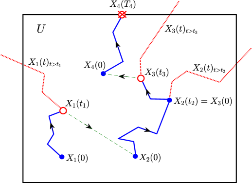
6 Synchronous and asynchronous computing

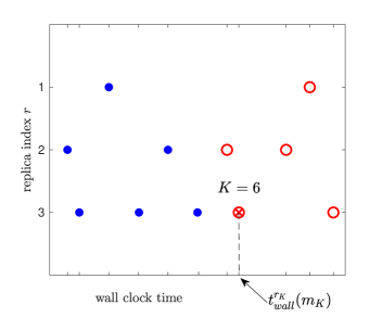
Recall that the speedup in ParRep comes from computing the trajectory fragments $X_{m}(t)_{0\leq t\leq t_{m}}$ partly or fully in parallel. These fragments must be ordered, via the index $m\geq 1$, to obtain the long trajectory pictured in Figure 1. Below, we explore two possible ways to order the fragments, depending on whether we want to employ synchronous or asynchronous computing. In the former case, we have in mind a computing environment consisting of $R$ processors that are nearly synchronous. In the latter case we consider an arbitrary number of processors that potentially have widely different performance.

Below, we will consider only fragments of constant time length, $t_{m}\equiv\Delta t$. For synchronous computing, following ideas from [3, 5, 65], we consider the ordering of trajectory fragments in Proposition 6.1 below.

Figure 2: An example of a synchronous ParRep algorithm based on the ordering of fragments in Proposition 6.1. Solid dots and hollow circles correspond to fragments’ initial and terminal points. The cross corresponds to the terminal point of the first fragment, in terms of the ordering, to escape from $U$. Times of copies that contribute to $g_{par}$ and $T_{par}$ are pictured with solid line segments and solid dots, while times that do not contribute are pictured with dotted lines and hollow circles.

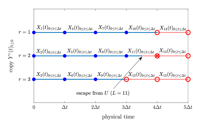
Proposition 6.1 (Synchronous computing).

Suppose $Y^{r}(t)_{t\geq 0}$, $r=1,\ldots,R$, are independent copies of $X(t)_{t\geq 0}$ with ${\mathcal{L}}(X(0))=\rho$. Let $m_{k}=\lfloor(k-1)/R\rfloor$ and $r_{k}=k-R\lfloor(k-1)/R\rfloor$, and for $k\geq 1$ define trajectory fragments $X_{k}(t)_{0\leq t\leq\Delta t}$ by

(5) $$X_{k}(t)=Y^{r_{k}}(m_{k}\Delta t+t),\qquad 0\leq t\leq\Delta t.$$

Then Assumption 5.1 holds with an appropriate definition of the trajectory fragments’ irrelevant futures. Thus the conclusions of Theorem 5.2 and 5.3 hold.

Figure 2 shows the trajectory fragments defined in (5).

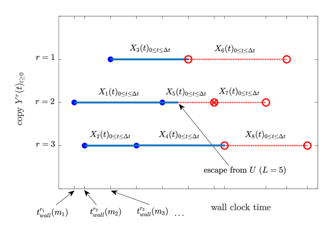
In asynchronous computing, perhaps the most natural ordering is the wall-clock ordering: the fragments are ordered according to the wall-clock time that their starting points are computed. See Figure 3. When does the wall-clock ordering satisfy Assumption 5.1? Note that (3) simply says that each fragment evolves forward in time independently of the preceding fragments and their irrelevant futures. This condition is easy to establish with an appropriate choice of the irrelevant futures. Ensuring (4) holds is more subtle. We will show, however, that if the wall-clock time it takes to compute each fragment depends on processor variables, but not on the fragments themselves, then the wall-clock time ordering is independent of the fragments and (4) holds.

We will distinguish between a wall-clock time and a physical time, where the former is self-explanatory and the latter refers to the time index $t$ of a copy of $X(t)_{t\geq 0}$. Let $Y^{r}(t)_{t\geq 0}$ be independent copies of $X(t)_{t\geq 0}$ starting at independent samples of the QSD $\rho$. The wall-clock time ordering of fragments satisfies Assumption 5.1 above if (i) the wall-clock times are independent of the physical times, (ii) the wall-clock time to compute copy $Y^{r}(t)_{t\geq 0}$ is an increasing function of the physical time, and (iii) two processors never finish at exactly the same wall-clock time, so that the wall-clock times can be given a unique ordering. Write $t_{wall}^{r}(m)$ for the wall-clock time it takes to compute $Y^{r}(t)_{t\geq 0}$ up to physical time $t=m\Delta t$. Proposition 6.2 below makes the claims above precise:

Figure 3: An example of an asynchronous ParRep algorithm based on wall-clock time ordering of fragments in Proposition 6.2. Solid dots and hollow circles correspond to fragments’ initial and terminal points. The cross corresponds to the terminal point of the first fragment, in terms of the ordering, to escape from $U$. Times of copies that contribute to $g_{par}$ and $T_{par}$ are pictured with solid line segments and solid dots, while times that do not contribute are pictured with dotted lines and hollow circles.

Proposition 6.2 (Asynchronous computing).

Suppose $Y^{r}(t)_{t\geq 0}$, $r=1,\ldots,R$, are independent copies of $X(t)_{t\geq 0}$ with ${\mathcal{L}}(X(0))=\rho$. Assume $(t_{wall}^{r}(m)_{m\geq 0})^{1\leq r\leq R}$ are nonnegative random numbers such that:

• $(t_{wall}^{r}(m)_{m\geq 0})^{1\leq r\leq R}$ is independent of $(Y^{r}(t)_{t\geq 0})^{1\leq r\leq R}$;

• Almost surely, $t_{wall}^{r}(m)\leq t_{wall}^{r}(n)$ when $m\leq n$ and $1\leq r\leq R$;

• Almost surely, there is a unique sequence $(r_{k},m_{k})_{k\geq 1}$ such that:

  $$(r_{k},m_{k})_{k\geq 1}\text{ has range }\{1,\ldots,R\}\times\{0,1,2,\ldots\}\qquad\text{(surjectivity)},$$

  $$t_{wall}^{r_{1}}(m_{1})<t_{wall}^{r_{2}}(m_{2})<t_{wall}^{r_{3}}(m_{3})<\ldots\qquad\qquad\text{(monotonicity)}.$$

For $k\geq 1$ define trajectory fragments $X_{k}(t)_{0\leq t\leq\Delta t}$ by

(6) $$X_{k}(t)=Y^{r_{k}}(m_{k}\Delta t+t),\qquad 0\leq t\leq\Delta t.$$

Then Assumption 5.1 holds with an appropriate definition of the trajectory fragments’ irrelevant futures. Thus the conclusions of Theorems 5.2 and 5.3 hold.

Figure 3 shows the trajectory fragments $X_{m}(t)_{0\leq t\leq t_{m}}$ defined in (6).

Assumptions (ii) and (iii) are quite natural, but assumption (i) can fail in many very ordinary settings. We sketch an example explaining how this could happen. Suppose $U=(0,1)\subseteq{\mathbb{R}}$ and say $X(t)_{t\geq 0}$ obeys some one dimensional stochastic differential equation. Suppose we use an integrator for $X(t)_{t\geq 0}$ that is slow near $0$ but fast near $1$. Then the wall-clock ordering will likely put trajectory fragments that are near $1$ ahead of those near $0$. This bias in the ordering would in turn create a bias toward escaping through $1$: in Algorithm 1, we would expect that ${\mathbb{P}}(X_{par}=1)>{\mathbb{P}}(X_{T}=1)$, where $X_{T}$ is the correct escape point. We construct a specific example demonstrating this bias in Remark 10.15 in Section 10.1 below.

The speed of integrators does commonly depend on position in space, particularly when the time step varies to account for numerical stiffness [55]. This is an important caveat to keep in mind for asynchronous algorithms. This issue has not been explored much in the literature; see however brief discussions in [30] and [46].

The setting of Parsplice [46, 47, 54] is slightly different from the above. In ParSplice, a splicer tells a producer to generate fragments among several metastable sets. The splicer distributes the fragments according to where it speculates that they will be needed. These fragments are given a label as soon as they are assigned, and this label never changes. The labels are assigned in wall-clock time order. Thus label $i$ is less than label $j$ if and only if the splicer tells the producer to generate fragment $i$ before it tells the producer to generate fragment $j$. When the splicer tells the producer to generate a fragment in a particular metastable set $U$, it takes as its starting point the terminal point of the fragment in $U$ with the smallest label. Crucially, this label is smallest among all fragments in $U$ and not just among fragments in $U$ which have been fully computed at the current wall-clock time. Thus, the ordering of fragments in $U$, fixed by the splicer, can be seen as independent of the fragments themselves, and the arguments above demonstrate consistency of ParSplice.

7 PDMPs

The remainder of this article will focus on applying our ideas above to PDMPs. We begin with a brief informal description of PDMPs. A PDMP is a càdlàg process consisting of a deterministic dynamics interrupted by jumps at random times; formally, a PDMP in ${\mathbb{R}}^{d}$ has a generator $L$ of the form

(7) $$Lf(z)=\partial_{\Gamma(z)}f(z)+\lambda(z)\int(f(z^{\prime})-f(z))Q(z,dz^{\prime})$$

acting on suitable $f:{\mathbb{R}}^{d}\to{\mathbb{R}}$. Here $\lambda(z)$ is the jump rate at $z\in{\mathbb{R}}^{d}$, a Markov kernel $Q(z,dz^{\prime})$ describes the jump distribution, and $\Gamma$ defines the deterministic flow

$$\partial_{t}\psi(t,z)=\Gamma(\psi(t,z)),\qquad\psi(0,z)=z.$$

Write $\theta_{0}+\ldots+\theta_{n-1}$ for the $n$th jump time, so that $\theta_{n-1}$ is the holding time before the $n$th jump, and write $\xi_{n}$ for the position immediately after the $n$th jump, with $\xi_{0}$ the initial position. Then the PDMP generated by (7) is described by $\psi$ together with $(\xi_{n},\theta_{n})_{n\geq 0}$; we call the latter the skeleton chain of $Z(t)_{t\geq 0}$. Note that the skeleton chain is a time homogeneous Markov chain.

For convenience we describe a way to simulate a PDMP described by (7) in Algorithm 8 below. In the algorithm, we abuse notation by writing $\theta_{n}$, $\xi_{n}$, and $Z(t)$ for particular realizations of these random objects.

Algorithm 2 Simulating a PDMP

Starting from an initial point $\xi_{0}$ and time $t=0$, set $n=0$, and iterate:

1. Sample $\theta_{n}$ according to the distribution

(8) $${\mathbb{P}}(\theta_{n}>r)=\exp\left(-\int_{0}^{r}\lambda(\psi(s,\xi_{n}))\,ds\right).$$

2. Set $Z(t+s)=\psi(s,\xi_{n})$ for $s\in[0,\theta_{n})$, and sample $\xi_{n+1}$ from $Q(Z(t+\theta_{n}^{-}),dz)$.

3. Update $t\leftarrow t+\theta_{n}$ and then $n\leftarrow n+1$. Then return to Step 1.

Steps 1-3 above define a realization of $Z(t)_{t\geq 0}$ with skeleton chain $(\xi_{n},\theta_{n})_{n\geq 0}$.

Sampling the times $\theta_{n}$ is a nontrivial task, but there are efficient methods based on Poisson thinning [6, 59] and identifying certain critical points along the flow direction [26]. See also [59] for other methods to simulate a PDMP, including some based on time discretization. We will always assume our initial points $(\xi_{0},\theta_{0})$ are chosen so that $\theta_{0}$ satisfies (8) for $n=0$, so that we can skip the first step in Algorithm 8.

7.1 Example: linear flow

Consider a PDMP with deterministic paths that are lines in ${\mathbb{R}}^{d-1}$ corresponding to a finite collection of velocity vectors $d_{i}\in{\mathbb{R}}^{d-1}$, $i\in{\mathcal{I}}\subseteq{\mathbb{N}}$. Its generator $L$ is defined on suitable functions $f:{\mathbb{R}}^{d-1}\times{\mathcal{I}}\to{\mathbb{R}}$ by

(9) $$Lf(x,i)=d_{i}\cdot\nabla f(x,i)+\sum_{j\neq i}\lambda_{j}(x,i)(f(x,j)-f(x,i)),$$

where $\lambda_{j}(x,i)\geq 0$ for $j\neq i$. Suppose we want to sample the probability density

(10) $$Z^{-1}e^{-V(x)},\qquad Z=\int e^{-V(x)}\,dx,$$

where $V:{\mathbb{R}}^{d-1}\to{\mathbb{R}}$ is smooth and grows sufficiently fast at $\infty$ so that $Z<\infty$. For the PDMP generated by (9) to have an invariant probability density independent of $i$ and proportional to (10), the jump rates must satisfy

(11) $$\sum_{j\neq i}\left(\lambda_{i}(x,j)-\lambda_{j}(x,i)\right)=-d_{i}\cdot\nabla V(x).$$

See Remark 10.17 in Section 10.1 below, and [6] for a similar calculation.

Event Chain Monte Carlo and the Zig-Zag process fit into this framework. And while these methods were designed for efficient sampling, we argue that they may be limited in certain situations. To see why, note that (11) says that at $x$, the rate into $d_{i}$ minus the rate out of $d_{i}$ equals minus the gradient of $V$ in direction $d_{i}$. Thus the PDMP is likely to change directions when it moves up a steep slope of $V$. This suggests the PDMP can struggle to escape from a basin of attraction of $V$, defined as the set of initial conditions $x(0)$ for which $dx(t)/dt=-\nabla V(x(t))$ has a unique long-time limit.

8 ParRep for PDMPs

In this section $Z(t)_{t\geq 0}$ is a PDMP with stationary distribution $\pi$, and $f$ is a real-valued function defined on the state space of $Z(t)_{t\geq 0}$. Below we outline some ParRep algorithms for estimating coarse dynamics as well as stationary averages, with a focus on the latter. The stationary average of $f$ is

(12) $$\langle f\rangle=\int f(x)\pi(dx).$$

Algorithms 5 and 8 below are ParRep algorithms based on the skeleton chain and the continuous time PDMP, respectively. Algorithms 3 and 6 are parallel steps for synchronous computing, while Algorithms 4 and 7 are for asynchronous computing. Algorithms 3 and 6, which are essentially extensions to PDMPs of algorithms recently proposed for continuous time Markov chains [64, 65], use the ordering of trajectory fragments defined in Proposition 6.1. Algorithms 4 and 7 employ the wall-clock time ordering of fragments from Proposition 6.2. We prove consistency of all of our parallel steps via our trajectory fragment framework.

We do not attempt to prove existence, uniqueness or convergence to the QSD for general PDMPs. Instead we refer the reader to recent articles [14, 15] for conditions which ensure convergence to a unique QSD. From those works, under appropriate assumptions, one can establish convergence to a unique QSD in $D\times{\mathcal{I}}\subseteq{\mathbb{R}}^{d}$ for a PDMP generated by (9). For instance, exponential convergence is guaranteed if $D\subseteq{\mathbb{R}}^{d-1}$ is an open connected bounded domain and there exist $m,M$ so that $0<m\leq\lambda_{j}(x,i)\leq M$ for all $x\in D$ and $i,j\in{\mathcal{I}}$: see [14], pg. 261. Similar arguments can be made for the QSD of the skeleton chain. Even without theoretical guarantees, in practice, one can empirically validate convergence to the QSD using certain diagnostics; see for instance [8].

8.1 Skeleton chain-based parrep algorithm

Let ${\mathcal{W}}$ be the collection of metastable sets for the skeleton chain $(\xi_{n},\theta_{n})_{n\geq 0}$. For instance, if $Z(t)_{t\geq 0}$ has generator similar to the form (9) and we want to sample from the distribution (10), it is natural to define ${\mathcal{W}}$ in terms of basins of attraction of $V$, in which case elements of ${\mathcal{W}}$ may be identified on the fly by gradient descent [62, 63]. See Section 9 for an example of metastable sets defined this way.

Assumption 8.1.

$(\xi_{n},\theta_{n})_{n\geq 0}$ has a QSD $\nu=\nu_{W}$ in each $W\in{\mathcal{W}}$ satisfying

$$\nu(A)=\lim_{n\to\infty}{\mathbb{P}}((\xi_{n},\theta_{n})\in A|(\xi_{m},\theta_{m})\in W,\,0\leq m\leq n)\quad\forall\,A\subseteq W.$$

For simpler notation, we do not explicitly indicate the dependence of $\nu$ on $W$.

Algorithm 3 Synchronous skeleton chain parallel step in $W$

1. Generate iid samples $(\xi_{0}^{r},\theta_{0}^{r})^{r=1,\ldots,R}$ from the QSD $\nu$ in $W$. Using these as starting points, independently evolve $R$ copies $((\xi_{n}^{r},\theta_{n}^{r})_{n\geq 0})^{r=1,\ldots,R}$ of the skeleton chain.

2. Let $N=\inf\{n:\exists\,r\,s.t.\,(\xi_{n}^{r},\theta_{n}^{r})\notin W\}$, $J=\min\{r:(\xi_{N}^{r},\theta_{N}^{r})\notin W\}$, and define

$$f_{par}=\sum_{n=0}^{N-2}\sum_{r=1}^{R}\int_{0}^{\theta_{n}^{r}}f(\psi(t,\xi_{n}^{r}))\,dt+\sum_{r=1}^{J}\int_{0}^{\theta_{N-1}^{r}}f(\psi(t,\xi_{N-1}^{r}))\,dt$$

and $T_{par}={\mathbbm{1}}_{par}$ by using the same formula but with ${\mathbbm{1}}(z)\equiv 1$ in place of $f$. Set

$$(\xi_{par},\theta_{par})=(\xi_{N}^{J},\theta_{N}^{J}).$$

Once $f_{par}$, $T_{par}$ and $(\xi_{par},\theta_{par})$ can be computed, the parallel step is complete.

Algorithm 4 Asynchronous skeleton chain parallel step in $W$

1. Generate iid samples $(\xi_{0}^{r},\theta_{0}^{r})^{r=1,\ldots,R}$ from the QSD $\nu$ in $W$. Using these as starting points, independently evolve $R$ copies $((\xi_{n}^{r},\theta_{n}^{r})_{n\geq 0})^{r=1,\ldots,R}$ of the skeleton chain.

2. Reorder these skeleton chain points in the order they are computed in wall-clock time, i.e. as $(\xi_{m_{k}}^{r_{k}},\theta_{m_{k}}^{r_{k}})_{k\geq 1}$ where $t_{wall}^{r_{1}}(m_{1})\leq t_{wall}^{r_{2}}(m_{2})\leq\ldots$ and $t_{wall}^{r}(n)$ is the wall-clock time it takes to compute the skeleton chain $(\xi_{m}^{r},\theta_{m}^{r})_{m\geq 0}$ up to physical time $m=n$. Set $\sigma^{r}=\inf\{m:(\xi_{m}^{r},\theta_{m}^{r})\notin W\}$, $K=\inf\{k:\sigma^{r_{k}}\leq m_{k}+1\}$, and

$$f_{par}=\sum_{k=1}^{K}\int_{0}^{\theta_{m_{k}}^{r_{k}}}f(\psi(t,\xi_{m_{k}}^{r_{k}}))\,dt.$$

Define $T_{par}={\mathbbm{1}}_{par}$ by using the same formula but with ${\mathbbm{1}}(z)\equiv 1$ in place of $f$. Let

$$(\xi_{par},\theta_{par})=(\xi_{\sigma^{r_{K}}}^{r_{K}},\theta_{\sigma^{r_{K}}}^{r_{K}}).$$

Once $f_{par}$, $T_{par}$ and $(\xi_{par},\theta_{par})$ can be computed, the parallel step is complete.

Algorithms 3 and 4 are parallel steps designed for synchronous and asynchronous computing, respectively. See Figure 4 for a diagram of both parallel steps. The first step in Algorithm 3 and Algorithm 4 – called dephasing in the literature [3, 5, 62, 65] – involves generating $R$ independent samples from the QSD $\nu$ in $W$. These QSD samples may be obtained in a variety of ways. One option is to do rejection sampling using independent copies of the skeleton chain: whenever a copy escapes from $W$, start it afresh in $W$ until each copy has remained in $W$ for a long enough consecutive time. Another possibility is based on the Fleming-Viot branching process [8, 24]: when a copy escapes from $W$, restart it at the current position of a copy still in $W$ chosen at random. For more discussion see [8, 52, 62].

Figure 4: Illustration of the parallel steps used in Algorithm 5. The number of copies, or parallel replicas, is $R=3$. The cross indicates an escape from $W$. Time steps of copies of the skeleton chain that contribute to $f_{par}$ and $T_{par}$ are pictured with solid dots, while time steps that do not contribute are pictured with hollow circles. Left: The synchronous parallel step, Algorithm 3. Copy $r=2$ escapes from $W$ at skeleton chain time $3$. In this example $N=3$ and $J=2$. Right: The asynchronous parallel step, Algorithm 4. Copy $r=3$ is the first to escape from $W$ in terms of the wall-clock time ordering. It escapes at wall-clock time $t_{wall}^{r_{K}}(m_{K})$. In this example $K=6$.

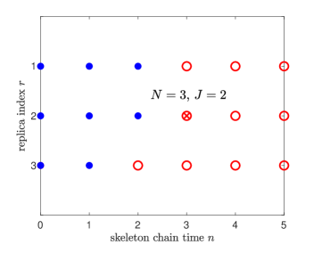
Recall the speedup from ParRep comes from the parallel step. The speedup – the factor by which ParRep reduces the wall-clock computation time, compared to serial simulation of a trajectory of the same physical time – can be a factor of up to $R$, the number of copies or replicas [3, 5, 30, 62, 65], when Algorithm 8 is used to simulate the skeleton chain. See Figure 7. The parallel step is consistent no matter the choice of $W$, but if $W$ is not metastable there may be no gain in efficiency, as too much computation time will be spent sampling the QSD.

Algorithm 5 Skeleton chain computation of stationary averages

Choose an initial point $(\xi_{0},\theta_{0})$, set $f_{sim}=0$, $T_{sim}=0$, and iterate:

1. Starting at $(\xi_{0},\theta_{0})$, evolve $(\xi_{n},\theta_{n})_{n\geq 0}$ forward in time, stopping at time

$$L=\inf\{n\geq T_{corr}^{\nu}(W)-1:\exists\,W\in{\mathcal{W}}\,s.t.\,(\xi_{n-k},\theta_{n-k})\in W,\,k=0,\ldots,T_{corr}^{\nu}(W)-1\},$$

the first time it remains in some $W\in{\mathcal{W}}$ for $T_{corr}^{\nu}(W)$ consecutive time steps. Set

$$f_{decorr}=\sum_{n=0}^{L-1}\int_{0}^{\theta_{n}}f(\psi(t,\xi_{n}))\,dt$$

and $T_{decorr}={\mathbbm{1}}_{decorr}$ using the same formula. Store this $W$ for Step 2 and update

$$f_{sim}\leftarrow f_{sim}+f_{decorr},\qquad T_{sim}\leftarrow T_{sim}+T_{decorr}.$$

2. Run the parallel step (Algorithm 3 or 4) in the set $W$ from Step 1. Update $f_{sim}\leftarrow f_{sim}+f_{par}$, $T_{sim}\leftarrow T_{sim}+T_{par}$, $(\xi_{0},\theta_{0})=(\xi_{par},\theta_{par})$, and return to Step 1.

The algorithm stops when $T_{sim}$ exceeds a user-chosen threshold $T_{stop}$. At this time,

$$\langle f\rangle\approx\frac{f_{sim}}{T_{sim}}$$

is our estimate of the stationary average (12).

Theorem 8.2 gives conditions that establish consistency of Algorithm 3 and 4. For Algorithm 4, the crucial condition is that the wall-clock times it takes for the processors to compute steps of the skeleton chains are independent of those chains. Whether this holds true will depend on the algorithm used to simulate the PDMP. If it is a time discretization-based algorithm, or an implementation of Algorithm 8 based on Poisson thinning, then the computational effort to obtain one step of the skeleton chain can be larger in regions in state space with lower jump rates. For CTMCs simulated via the SSA/Gillespie algorithm [2], the effort to simulate one step of the skeleton chain may be essentially independent of the position of the chain.

Theorem 8.2 (Consistency of the parallel steps Algorithm 3 and 4).

(i) Let $\nu$ be the QSD of $(\xi_{n},\theta_{n})_{n\geq 0}$ in some $W\in{\mathcal{W}}$, suppose that ${\mathcal{L}}(\xi_{0},\theta_{0})=\nu$, and define $M=\inf\{n\geq 0:(\xi_{n},\theta_{n})\notin W\}$. Then in Algorithm 3,

(13) $${\mathbb{E}}(f_{par})={\mathbb{E}}\left(\sum_{n=0}^{M-1}\int_{0}^{\theta_{n}}f(\psi(t,\xi_{n}))\,dt\right)$$

and

(14) $$(\xi_{par},\theta_{par})\stackrel{{\scriptstyle\mathcal{L}}}{{=}}(\xi_{M},\theta_{M}).$$

(ii) Suppose $(t_{wall}(m)_{m\geq 0})^{1\leq r\leq R}$, the wall-clock times from Algorithm 4, satisfy the assumptions of Proposition 6.2 when $(Y^{r}(t)_{t\geq 0})^{r=1,\ldots,R}$ equals $((\xi_{n}^{r},\theta_{n}^{r})_{n\geq 0})^{r=1,\ldots,R}$. Adopt the assumptions in (i) above. Then (13)-(14) hold.

The times $T_{corr}^{\nu}(W)$ in Algorithm 5 may be chosen on the fly, or they may be set at the beginning of simulations. Choosing an appropriate value may be done using various convergence diagnostics or a priori information; see [8, 52, 62] for details.

Consistency of the parallel steps, together with exactness of the decorrelation step, show that Algorithm 5 produces correct stationary averages, provided some mild recurrence assumptions hold [3]. The reason is essentially the law of large numbers: for computations of stationary averages, due to repeated visits to each metastable set, in the parallel steps it is enough to get contributions $f_{par}$ to $f_{sim}$ with the correct average value along with escape events with the correct law.

We do not attempt here to prove ergodicity using this argument, but mention it has been studied previously in [3, 65]. Our numerical simulations in Section 9 below also support its validity. One interesting aspect of the parallel step is that the averaging over independent copies or replicas can be considered a bonus, as it likely lowers the variance of the estimate $f_{sim}/T_{sim}\approx\langle f\rangle$ of the stationary average, compared to an estimate from a serial trajectory of physical time length $T_{sim}$.

8.2 Continuous time PDMP-based algorithm

Let ${\mathcal{V}}$ be the collection of metastable sets for $Z(t)_{t\geq 0}$. As above, if $Z(t)_{t\geq 0}$ has a generator similar to (9) and we want to sample from the distribution (10), the elements of ${\mathcal{V}}$ can be defined in terms of the basins of attraction of $V$. We will require a time interval $\Delta t>0$, which is not necessarily a time step for discretizing the PDMP. For instance, $\Delta t$ could be a polling time for resynchronizing parallel processors.

Algorithm 6 Synchronous continuous time parallel step in $W$

1. Generate iid samples $Z^{r}(0)^{r=1,\ldots,R}$ from the QSD $\mu$ in $W$. Using these as starting points, independently evolve $R$ copies $(Z^{r}(t)_{t\geq 0})^{r=1,\ldots,R}$ of the PDMP.

2. Let $\tau^{r}=\inf\{t:Z^{r}(t)\notin W\}$, set

$$N=\inf\{n\in{\mathbb{N}}:\exists\,r\,s.t.\,\tau^{r}\leq n\Delta t\},\qquad J=\min\{r:\tau^{r}\leq N\Delta t\},$$

and define

$$f_{par} =\sum_{n=1}^{N-1}\sum_{r=1}^{R}\int_{(n-1)\Delta t}^{n\Delta t}f(Z^{r}(t))\,dt$$

$$\qquad\qquad+\sum_{r=1}^{J-1}\int_{(N-1)\Delta t}^{N\Delta t}f(Z^{r}(t))\,dt+\int_{(N-1)\Delta t}^{\tau^{J}}f(Z^{J}(t))\,dt,$$

and $T_{par}={\mathbbm{1}}_{par}$ by using the same formula but with ${\mathbbm{1}}(z)\equiv 1$ in place of $f$. Set

$$Z_{par}=Z^{J}(\tau^{J}).$$

Once $f_{par}$, $T_{par}$ and $Z_{par}$ can be computed, the parallel step is complete.

Algorithm 7 Asynchronous continuous time parallel step in $W$

1. Generate iid samples $Z^{r}(0)^{r=1,\ldots,R}$ from the QSD $\mu$ in $W$. Using these as starting points, independently evolve $R$ copies $(Z^{r}(t)_{t\geq 0})^{r=1,\ldots,R}$ of the PDMP.

2. Reorder the $\Delta t$ time intervals of these copies in the order they are computed in wall-clock time, i.e. as $Z^{r_{k}}(m_{k}\Delta t)_{k\geq 1}$ where $t_{wall}^{r_{1}}(m_{1})\leq t_{wall}^{r_{2}}(m_{2})\leq\ldots$ and $t_{wall}^{r}(n)$ is the wall-clock time it takes to compute the PDMP $Z^{r}(t)_{t\geq 0}$ up to physical time $t=n\Delta t$. Set $\tau^{r}=\inf\{t:Z^{r}(t)\notin W\}$, $K=\inf\{k:\tau^{r_{k}}\leq(m_{k}+1)\Delta t\}$, and

$$f_{par}=\sum_{k=1}^{K-1}\int_{m_{k}\Delta t}^{(m_{k}+1)\Delta t}f(Z^{r_{k}}(t))\,dt+\int_{m_{K}\Delta t}^{\tau^{r_{K}}}f(Z^{r_{K}}(t))\,dt$$

and $T_{par}={\mathbbm{1}}_{par}$ by using the same formula but with ${\mathbbm{1}}(z)\equiv 1$ in place of $f$. Let

$$Z_{par}=Z^{r_{K}}(\tau^{r_{K}}).$$

Once $f_{par}$, $T_{par}$ and $\xi_{par}$ can be computed, the parallel step is complete.

We will adopt the following assumption.

Assumption 8.3.

$Z(t)_{t\geq 0}$ has a QSD $\mu=\mu_{W}$ in each $W\in{\mathcal{V}}$ satisfying

$$\mu(A)=\lim_{t\to\infty}{\mathbb{P}}(Z(t)\in A|Z(s)\in W,\,0\leq s\leq t)\quad\forall\,A\subseteq W.$$

We do not explicitly indicate the dependence of $\mu$ on $W$. Notice the QSD of the PDMP is different from that of its skeleton chain in general.

Algorithms 6 and 7 are parallel steps designed for synchronous and asynchronous computing, respectively; see Figure 5. The first step in Algorithm 6 and Algorithm 7 – the dephasing step – involves generating $R$ independent samples from the QSD $\mu$ in $W$. Note that this is the QSD of the PDMP in $W$, not the QSD of its skeleton chain. The QSD samples can be obtained exactly as described in the previous section, but with the PDMP taking the place of the skeleton chain.

Figure 5: Illustration of the parallel steps used in Algorithm 8. The number of copies, or parallel replicas, is $R=3$. Solid dots and hollow circles correspond to trajectories at PDMP times $n\Delta t$. The cross indicates the terminal point of a $\Delta t$-time interval corresponding to an escape from $W$. Times of copies that contribute to $g_{par}$ and $T_{par}$ are pictured with solid line segments and solid dots, while times that do not contribute are pictured with dotted lines and hollow circles. Left: The synchronous parallel step, Algorithm 6. Copy $r=2$ escapes at PDMP time $\tau^{2}$. In this example $N=4$ and $J=2$. Right: The asynchronous parallel step, Algorithm 7. Copy $r=2$ is the first to escape in terms of the wall-clock time ordering. The notches on the wall-clock time axis are the values of $t_{wall}^{r_{k}}(m_{k})$, $k=1,\ldots,11$. In this example $K=5$.

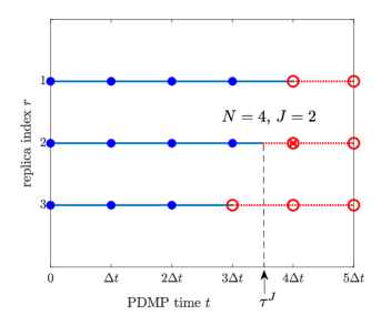
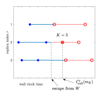
The speedup from the parallel step can be up to a factor of $R$, the number of copies or replicas [5, 3, 30, 62, 65], provided the underlying PDMP simulation algorithm is based on time discretization. If the PDMP simulation algorithm is based on computing the skeleton chain, then the speedup in Algorithm 6 may be reduced. This can be mitigated, however, by using Algorithm 7 instead. The parallel step is consistent for any $W$, with a speedup if $W$ is metastable for the PDMP.

Theorem 8.4 gives conditions that establish consistency of the parallel steps, Algorithm 6 and 7. For the asynchronous parallel step, the crucial condition essentially says that the wall-clock time it takes to compute a $\Delta t$ time interval of $Z(t)_{t\geq 0}$ is independent of its position. This is reasonable if $Z(t)_{t\geq 0}$ is simulated via a time discretization technique with a fixed time step. It may not be reasonable if a skeleton chain-based technique, like Algorithm 8, is used instead.

Algorithm 8 Continuous time computation of stationary averages

Choose an initial point $Z(0)$, set $f_{sim}=0$, $T_{sim}=0$, and iterate:

1. Starting at $Z(0)$, evolve $Z(t)_{t\geq 0}$ forward in time, stopping at time

$$S=\inf\{t\geq T_{corr}^{\mu}(W):\exists\,W\in{\mathcal{V}}\,s.t.\,Z(s)\in W,\,s\in[t-T_{corr}^{\mu}(W),t]\},$$

the first time it remains in some $W\in{\mathcal{V}}$ for consecutive time $T_{corr}^{\mu}(W)$. Set

$$f_{decorr}=\int_{0}^{S}f(Z(t))\,dt$$

and $T_{decorr}={\mathbbm{1}}_{decorr}$ using the same formula. Store this $W$ for Step 2 and update

$$f_{sim}\leftarrow f_{sim}+f_{decorr},\qquad T_{sim}\leftarrow T_{sim}+T_{decorr}.$$

2. Run the parallel step (Algorithm 6 or 7) in the set $W$ from Step 1. Update $f_{sim}\leftarrow f_{sim}+f_{par}$, $T_{sim}\leftarrow T_{sim}+T_{par}$, set $Z(0)=Z_{par}$, and then go to Step 1.

The algorithm stops when $T_{sim}$ exceeds a user-chosen threshold $T_{stop}$. At this time,

$$\langle f\rangle\approx\frac{f_{sim}}{T_{sim}}$$

is our estimate of the stationary average (12).

Theorem 8.4 (Consistency of the parallel steps Algorithm 6 and 7).

(i) Let $\mu$ be the QSD of $Z(t)_{t\geq 0}$ in some $W\in{\mathcal{V}}$, suppose that ${\mathcal{L}}(Z(0))=\mu$, and define $\tau=\inf\{t\geq 0:Z(t)\notin W\}$. Then in Algorithm 6,

(15) $${\mathbb{E}}(f_{par})={\mathbb{E}}\left(\int_{0}^{\tau}f(Z(t))\,dt\right)$$

and

(16) $$(T_{par},Z_{par})\stackrel{{\scriptstyle\mathcal{L}}}{{=}}(\tau,Z(\tau)).$$

(ii) Suppose $(t_{wall}(m)_{m\geq 0})^{1\leq r\leq R}$, the wall-clock times from Algorithm 7, satisfy the assumptions of Proposition 6.2 when $(Y^{r}(t)_{t\geq 0})^{r=1,\ldots,R}$ equals $(Z^{r}(t)_{t\geq 0})^{r=1,\ldots,R}$. Adopt the assumptions in (i) above. Then (15)-(16) hold.

Algorithm 8 generates correct stationary averages by the same argument as in the previous section. It is worth mentioning that Algorithms 6 and 7 have a property not shared by Algorithms 3 and 4: the escape events $(T_{par},Z_{par})$ in these parallel steps have the correct law for the PDMP. This allows us to use Algorithm 8 to compute the dynamics of $Z(t)_{t\geq 0}$. More precisely, Algorithm 8 leads to a PDMP dynamics that is correct on the quotient space obtained by considering each $W\in{\mathcal{V}}$ as a single point. Note that Algorithm 5 cannot be used in this way, as it generates dynamics of the skeleton chain and not the PDMP.

9 Numerics

Here we test our algorithms above on a toy PDMP model, our aim being to illustrate Algorithms 5 and 8. We will use these algorithms to sample the stationary average of a function $f$ with respect to the Boltzmann density $\pi=Z^{-1}e^{-\beta V}$, where $f$ and $V$ are defined below and $\beta>0$ is inverse temperature. The toy model is a two-dimensional version of a PDMP that may be defined in an arbitrary dimension $d-1$, as follows. Let $d_{0},\ldots,d_{N-1}\in{\mathbb{R}}^{d-1}$ be direction vectors such that $d_{0}+\ldots+d_{N-1}=0$. Let ${\mathbb{Z}}_{N}$ denote the integers modulo $N$, consider the indices of the $d_{k}$’s as elements of ${\mathbb{Z}}_{N}$, and for $k,\ell\in{\mathbb{Z}}_{N}$ define

$$F_{k,\ell}(x) =\beta(d_{k}+\ldots d_{k+\ell})\cdot\nabla V(x).$$

Figure 6: Contour plot of the potential $V$ in (18). $V$ has $4$ basins of attraction $W_{1},W_{2},W_{3},W_{4}$ of different depths, with $W_{1}$ the deepest. Recall a basin of attraction for $V$ is a set of initial conditions $x(0)$ for which the differential equation $dx(t)/dt=-\nabla V(x(t))$ has a unique long-time limit.

Consider the PDMP with generator defined by

(17) $$Lg(x,k)=d_{k}\cdot\nabla g(x,k)+\left[g(x,k-1)-g(x,k)\right]\max_{0\leq\ell\leq N-1}F_{k,\ell}(x)$$

for suitable $g:\Omega\times{\mathbb{Z}}_{N}\to{\mathbb{R}}$ where either $\Omega={\mathbb{R}}^{d-1}$ or $\Omega$ is a cube in ${\mathbb{R}}^{d-1}$ with periodic boundaries. This is the generator for a PDMP that, when moving in direction $d_{k}$ at point $x$, switches to direction $d_{k-1}$ with rate $\max_{0\leq\ell\leq N-1}F_{k,\ell}(x)$. The resulting process can be seen as a rejection-free or “lifted” version of the sequential Metropolis algorithm [29, 36], historically the first nonreversible sampling algorithm [27, 36] for sampling the Boltzmann distribution. Straightforward calculations show this PDMP has invariant density proportional to $\pi$; see Remark 10.19 in Section 10.1.

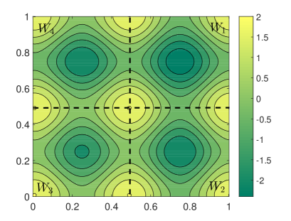
We consider the case where state space is $\Omega=[0,1]^{2}$ with periodic boundaries, $N=4$, $d_{0}=(1,0),\,d_{1}=(-1,0),\,d_{2}=(0,1),\,d_{3}=(0,-1)$, and the potential energy $V$ is pictured in Figure 6. Specifically

(18) $$V(x,y)=\cos(4\pi x)+\cos(4\pi y)+\frac{1}{5}\sin(2\pi x)+\frac{1}{5}\sin(2\pi y).$$

We define ${\mathcal{W}}$ and ${\mathcal{V}}$ using the basins of attraction $W_{i}$, $i=1,\ldots,4$ defined as the four squares of equal side length $1/2$ inside $[0,1]^{2}$. See Figure 6. Thus with $x$ and $k$ the position and direction variables, respectively, of the skeleton chain and PDMP, and $\theta$ the jump time variable of the skeleton chain,

$${\mathcal{W}} =\left\{\{(x,k,\theta):x\in W_{i},\,k\in\{0,1,2,3\},\,\theta>0\}:i=1,2,3,4\right\},$$

$${\mathcal{V}} =\left\{\{(x,k):x\in W_{i},\,k\in\{0,1,2,3\}\}:i=1,2,3,4\right\}.$$

That is, the skeleton chain or PDMP is in a given set in ${\mathcal{W}}$ or ${\mathcal{V}}$ at a particular time if and only if its position variable belongs to a given $W_{i}$ at that time.

Algorithm 9 Time discretization of the PDMP (17)

Choose an initial point $Z(0)\in{\mathbb{R}}^{d-1}\times\{0,\ldots,N-1\}$. and pick $d_{0},\ldots,d_{N-1}\in{\mathbb{R}}^{d-1}$ with $\sum_{k=0}^{N-1}d_{k}=0$. Choose a time step $\delta t>0$. Then set $t=0$ and iterate: 1. If $Z(t)=(x,k)$, define an acceptance probability

$$p=\min_{0\leq\ell\leq N-1}\exp\left(\beta V(x)-\beta V(x+d_{k}\delta t+\ldots+d_{k+\ell}\delta t)\right).$$

2. With probability $p$, set $Z(t+\delta t)=(x+d_{k}\delta t,k)$, else set $Z(t+\delta t)=(x,k-1)$.

3. Update $t\leftarrow t+\delta t$ and return to Step 1.

Here, $Z(n\delta t)_{n\geq 0}$ has invariant measure proportional to $e^{-\beta V}$; see Remark 10.21.

We tested Algorithm 5 and 8 with the synchronous parallel steps Algorithm 3 and Algorithm 6, respectively. We used both algorithms to estimate the stationary average $\langle f\rangle$ where $f(x,k)={\mathbbm{1}}_{x\in W_{1}}$, the characteristic function of the deepest basin of $V$. We used up to $R=100$ replicas and decorrelation times that were the same in each basin, $T_{corr}^{\nu}\equiv T_{corr}^{\nu}(W_{i})$ and $T_{corr}^{\mu}\equiv T_{corr}^{\mu}(W_{i})$, $i=1,\ldots,4$. We used Algorithm 9 with time step $\delta t=10^{-2}$ to simulate the PDMP. In Algorithm 8 we took $\Delta t=\delta t=10^{-2}$. The results are in Figures 7, 8 and 9.

Figure 7: Left: Time speedup vs. number of replicas, $R$, when $\beta=3$. Right: Time speedup vs. $\beta$ when $R=100$. In Algorithm 3 we used $T_{corr}^{\nu}=100$, while in Algorithm 6 we used $T_{corr}^{\mu}=6$. The decorrelation times were chosen so that Algorithm 3 and 6 would have similar values for the time speedup. Error bars for each data point were obtained from $50$ independent simulations, but they are smaller than the data markers. In the limit $\beta\to\infty$, the computational effort to sample the QSD vanishes compared to the effort to generate an escape event using serial simulation. In this limit, at left, we expect scaling like $R$ for finite $R$. On the other hand, at right, we expect the time speedup to level off at $R=100$ as $\beta\to\infty$. This figure is based on simulations performed by Peter Christman.

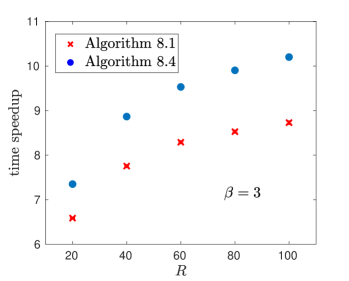
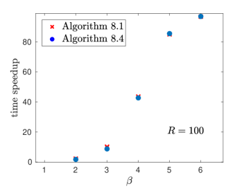
To analyze our results, we defined an idealized speedup factor as follows. Let $T^{R}$ be an idealized wall-clock time for a simulation of Algorithm 5 or 8 using the parallel steps Algorithm 3 and 6, respectively, up to a fixed time $T_{stop}$. The idealized wall-clock time $T^{R}$ is obtained by assuming that we use $R$ parallel processors with zero communication cost, such that on each processor, one step of the skeleton chain is computed in wall clock time $1$. Writing $T^{1}$ for the wall-clock time corresponding to $1$ processor or direct serial simulation, we define

$$\text{time speedup}=\frac{T^{R}}{T^{1}}.$$

We include computation time from the dephasing step – i.e. the QSD sampling step in Algorithms 3 and 6 – as part of $T^{R}$. We assume this dephasing is done using a Fleming-Viot-based technique as described above, with $R$ copies of the underlying skeleton chain or PDMP.

Processor communication, which we do not account for, of course takes a toll on the time speedup. However, the processor communication cost is small compared to the rest of the computational effort if the sets in ${\mathcal{W}}$ and ${\mathcal{V}}$ are significantly metastable. Thus, our time speedup gives a reasonable picture of the gain that can be expected.

The time speedup depends on the parameters in Algorithms 5 and 8. If all other parameters are held constant, the time speedup increases with $R$ or $\beta$, due to increasing parallelization or metastability, respectively (Figure 7), while the time speedup decreases with $T_{corr}^{\nu}$ and $T_{corr}^{\mu}$, due to increased effort to sample the QSD (Figure 8). With increasing metastability, the relative computational effort to sample the QSD decreases in comparison with the effort to simulate an escape from a metastable set. Since the latter is done in parallel, increasing the metastability leads to a larger time speedup.

Figure 8: Left: Time speedup vs. $T_{corr}^{\nu}$ in Algorithm 3. Right: Time speedup vs. $T_{corr}^{\mu}$ in Algorithm 6. In both plots $\beta=3$ and $R=100$. Error bars for each data point were obtained from $50$ independent simulations, but they are smaller than the data markers. This figure is based on simulations performed by Peter Christman.

Figure 9: Left: Approximation $f_{sim}/T_{sim}$ of the stationary average $\langle f\rangle$ using Algorithm 5. Right: Approximation $f_{sim}/T_{sim}$ of the stationary average $\langle f\rangle$ using Algorithm 8. In both plots $\beta=3$ and $R=100$, and simulations ran for $T_{sim}$ exceeding $10^{6}$. Error bars are empirical standard deviations obtained from $50$ independent simulations for each data point. The exact value $\langle f\rangle$ is indicated with a solid line. This figure is based on simulations performed by Peter Christman.

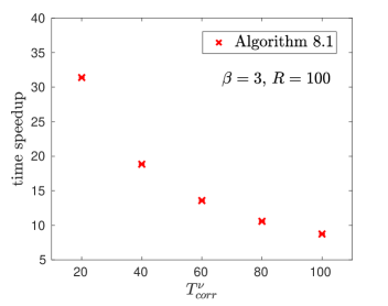
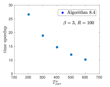
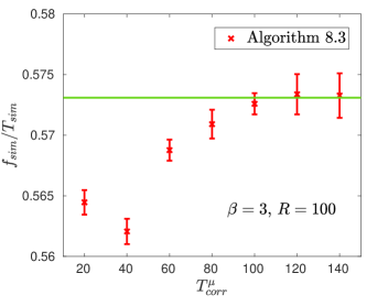
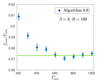
Figure 9 shows that the approximation $f_{sim}/T_{sim}$ approaches the stationary average $\langle f\rangle$ as the decorrelation times $T_{corr}^{\nu}$ and $T_{corr}^{\mu}$ increase, as expected. As discussed above, appropriate values of these QSD sampling times depend on the degree of metastability. Note that the approximations $f_{sim}/T_{sim}$ are quite good even for small QSD sampling times. This was true not just for $f(x,k)={\mathbbm{1}}_{x\in W_{1}}$ but for a variety of other functions. This feature, of reasonable accuracy in ParRep even for relatively small decorrelation times, was observed before in [64, 65]. Here this may be a result of the momentum-like direction variables, which can make the PDMP unlikely to immediately escape from a metastable set just after entering.

10 Proofs

Our first two results below, Proposition 10.1 and 10.3, establish the memoryless distribution of the escape time starting from the QSD, and the independence of the escape time and escape point, for general Markov processes. See for instance [16] for details. We include proofs for completeness.

Proposition 10.1.

Let $X(t)_{t\geq 0}$ have a QSD $\rho$ in $U$, and suppose ${\mathcal{L}}(X(0))=\rho$. Suppose $T=\inf\{t\geq 0:X(t)\notin U\}$ is finite almost surely. Then $T$ has a memoryless distribution; that is, $T$ is either exponentially or geometrically distributed.

Proof 10.2.

The definition (1) of the QSD together with the Markov property show that ${\mathcal{L}}(X(t+s)_{s\geq 0}|T>t)={\mathcal{L}}(X(s)_{s\geq 0})$. Thus, ${\mathbb{P}}(T>t+s|T>t)={\mathbb{P}}(T>s)$ for any $s,t\geq 0$. When $T$ is finite-valued, the only distribution satisfying this is

(19) $${\mathbb{P}}(T>t)=e^{-\lambda t}.$$

We use (19) to indicate either the (continuous) exponential distribution with parameter $\lambda>0$, or the (discrete) geometric distribution with parameter $p=1-e^{-\lambda}$.

Proposition 10.3.

Let $X(t)_{t\geq 0}$ have a QSD $\rho$ in $U$, and suppose ${\mathcal{L}}(X(0))=\rho$. Suppose $T=\inf\{t\geq 0:X(t)\notin U\}$ is finite almost surely. Then $T$ and $X(T)$ are independent.

Proof 10.4.

By Proposition 10.1, ${\mathbb{P}}(T>t)=e^{-\lambda t}$. For $A$ in the complement of $U$,

$${\mathbb{P}}(T\in((n-1)t,nt],X(T)\in A) ={\mathbb{P}}(T>(n-1)t,X(nt\wedge T)\in A)$$

$$={\mathbb{P}}(X(nt\wedge T)\in A|T>(n-1)t){\mathbb{P}}(T>(n-1)t)$$

$$={\mathbb{P}}(X(T)\in A,T\leq nt|T>(n-1)t){\mathbb{P}}(T>(n-1)t)$$

$$={\mathbb{P}}(X(T)\in A,T\leq t)e^{-\lambda(n-1)t},$$

where the last step uses (1). Summing over $n\geq 1$ establishes the result:

$${\mathbb{P}}(X(T)\in A) ={\mathbb{P}}(X(T)\in A,T\leq t)\frac{1}{1-e^{-\lambda t}}$$

$$=\frac{{\mathbb{P}}(X(T)\in A,T\leq t)}{{\mathbb{P}}(T\leq t)}.$$

Below, we write MGF for the moment generating function of a random variable. The results in Proposition 10.5 below hold in both continuous and discrete time. To connect the discrete and continuous time cases, we write $1-p=e^{-\lambda}$ where $p\in(0,1)$ is the geometric parameter and $\lambda>0$ is the exponential rate.

Proposition 10.5.

Let $t_{1},t_{2},\ldots$ be nonnegative deterministic times such that $\sum_{m=1}^{\infty}t_{m}=\infty$. Let $\tau_{1},\tau_{2},\ldots$ be random variables such that ${\mathbb{P}}(\tau_{1}>t)=e^{-\lambda t}$ and

(20) $${\mathbb{P}}(\tau_{m}>t|\tau_{m-1}>t_{m-1},\ldots,\tau_{1}>t_{1})=e^{-\lambda t},\quad m\geq 2.$$

Let $L=\inf\{m\geq 1:\tau_{m}\leq t_{m}\}$. Then

$${\mathbb{P}}(t_{1}+\ldots+t_{L-1}+\tau_{L}>t)=e^{-\lambda t}.$$

Proof 10.6.

Let $s_{m}=t_{1}+\ldots+t_{m}$ and $s_{0}=0$. By (20) and induction,

(21) $${\mathbb{P}}(\tau_{m}>t_{m},\ldots,\tau_{1}>t_{1})=e^{-\lambda(t_{1}+\ldots+t_{m})}=e^{-\lambda s_{m}}.$$

Using (20) again, in the continuous case,

(22) $$\begin{split}&{\mathbb{E}}\left(e^{u\tau_{m}}\mathbbm{1}_{\tau_{m}\leq t_{m}}|\tau_{m-1}>t_{m-1},\ldots,\tau_{1}>t_{1}\right)\\ &=\int_{0}^{t_{m}}e^{us}\lambda e^{-\lambda s}\,ds=\frac{\lambda}{u-\lambda}\left(e^{(u-\lambda)t_{m}}-1\right),\end{split}$$

while in the discrete case, where $e^{-\lambda}=1-p$,

(23) $$\begin{split}&{\mathbb{E}}\left(e^{u\tau_{m}}\mathbbm{1}_{\tau_{m}\leq t_{m}}|\tau_{m-1}>t_{m-1},\ldots,\tau_{1}>t_{1}\right)\\ &=\sum_{s=1}^{t_{m}}e^{us}e^{-\lambda(s-1)}(1-e^{-\lambda})=\frac{e^{u}-e^{u-\lambda}}{1-e^{u-\lambda}}\left(1-e^{(u-\lambda)t_{m}}\right).\end{split}$$

Note also that

(24) $$\{L=m\}=\{\tau_{m}\leq t_{m},\tau_{m-1}>t_{m-1},\ldots,\tau_{1}>t_{1}\}.$$

Consider the continuous case. Combining (21), (LABEL:MGF1) and (24) gives

(25) $$\begin{split}&{\mathbb{E}}\left(e^{u\tau_{m}}\mathbbm{1}_{L=m}\right)\\ &={\mathbb{E}}\left(e^{u\tau_{m}}\mathbbm{1}_{\tau_{m}\leq t_{m}}\mathbbm{1}_{\tau_{m-1}>t_{m-1},\ldots,\tau_{1}>t_{1}}\right)\\ &={\mathbb{E}}\left(e^{u\tau_{m}}\mathbbm{1}_{\tau_{m}\leq t_{m}}|{\tau_{m-1}>t_{m-1},\ldots,\tau_{1}>t_{1}}\right){\mathbb{P}}(\tau_{m-1}>t_{m-1},\ldots,\tau_{1}>t_{1})\\ &=\frac{\lambda}{u-\lambda}\left(e^{(u-\lambda)t_{m}}-1\right)e^{-\lambda s_{m-1}}.\end{split}$$

We now see that $s_{L-1}+\tau_{L}$ has the MGF of an exponential($\lambda$) random variable:

$${\mathbb{E}}\left(e^{u(s_{L-1}+\tau_{L})}\right) =\sum_{m=1}^{\infty}{\mathbb{E}}\left(e^{u(s_{L-1}+\tau_{L})}\mathbbm{1}_{L=m}\right)$$

$$=\sum_{m=1}^{\infty}e^{us_{m-1}}{\mathbb{E}}\left(e^{u\tau_{m}}\mathbbm{1}_{L=m}\right)$$

$$=\frac{\lambda}{u-\lambda}\sum_{m=1}^{\infty}\left(e^{(u-\lambda)s_{m}}-e^{(u-\lambda)s_{m-1}}\right)$$

$$=\frac{\lambda}{\lambda-u}\qquad\text{if }u<\lambda.$$

Similarly, in the discrete case, combining (21), (LABEL:MGF2) and (24) gives

(26) $$\begin{split}&{\mathbb{E}}\left(e^{u\tau_{m}}\mathbbm{1}_{L=m}\right)\\ &={\mathbb{E}}\left(e^{u\tau_{m}}\mathbbm{1}_{\tau_{m}\leq t_{m}}\mathbbm{1}_{\tau_{m-1}>t_{m-1},\ldots,\tau_{1}>t_{1}}\right)\\ &={\mathbb{E}}\left(e^{u\tau_{m}}\mathbbm{1}_{\tau_{m}\leq t_{m}}|{\tau_{m-1}>t_{m-1},\ldots,\tau_{1}>t_{1}}\right){\mathbb{P}}(\tau_{m-1}>t_{m-1},\ldots,\tau_{1}>t_{1})\\ &=\frac{e^{u}-e^{u-\lambda}}{1-e^{u-\lambda}}\left(1-e^{(u-\lambda)t_{m}}\right)e^{-\lambda s_{m-1}}.\end{split}$$

This shows again that $s_{L-1}+\tau_{L}$ has the MGF of a geometric($p$) random variable, via

$${\mathbb{E}}\left(e^{u(s_{L-1}+\tau_{L})}\right) =\sum_{m=1}^{\infty}{\mathbb{E}}\left(e^{u(s_{L-1}+\tau_{L})}\mathbbm{1}_{L=m}\right)$$

$$=\sum_{m=1}^{\infty}e^{us_{m-1}}{\mathbb{E}}\left(e^{u\tau_{m}}\mathbbm{1}_{L=m}\right)$$

$$=\frac{e^{u}-e^{u-\lambda}}{1-e^{u-\lambda}}\sum_{m=1}^{\infty}(e^{(u-\lambda)s_{m-1}}-e^{(u-\lambda)s_{m}})$$

$$=\frac{e^{u}-e^{u-\lambda}}{1-e^{u-\lambda}}\qquad\text{if }u<\lambda$$

$$=\frac{pe^{u}}{1-(1-p)e^{u}}\qquad\text{ if }u<-\log(1-p).$$

Proof 10.7 (Proof of Theorem 5.2).

Let $A$ be a subset of the complement of $U$. Note that, due to (3), the events $\{X_{m}(T_{m})\in A,T_{m}\leq t\}$ and $\{T_{m-1}>t_{m-1},\ldots,T_{1}>t_{1}\}$ are independent conditional on $\{X_{m}(0)=x\}$. Using this, (4) and Proposition 10.3,

(27) $$\begin{split}&{\mathbb{P}}(X_{m}(T_{m})\in A,T_{m}\leq t|T_{m-1}>t_{m-1},\ldots,T_{1}>t_{1})\\ &=\int{\mathbb{P}}(X_{m}(T_{m})\in A,T_{m}\leq t|X_{m}(0)=x,T_{m-1}>t_{m-1},\ldots,T_{1}>t_{1})\\ &\qquad\qquad\qquad\times{\mathbb{P}}(X_{m}(0)\in dx|T_{m-1}>t_{m-1},\ldots,T_{1}>t_{1})\\ &=\int{\mathbb{P}}(X_{m}(T_{m})\in A,T_{m}\leq t|X_{m}(0)=x)\rho(dx)\\ &={\mathbb{P}}(X(T)\in A,T\leq t)\\ &={\mathbb{P}}(X(T)\in A){\mathbb{P}}(T\leq t).\end{split}$$

Taking $A$ as the complement of $U$ in (LABEL:longprob), and using Proposition 10.1,

(28) $${\mathbb{P}}(T_{m}>t|T_{m-1}>t_{m-1},\ldots,T_{1}>t_{1})={\mathbb{P}}(T>t)=e^{-\lambda t},\quad\text{some }\lambda>0.$$

By (4), ${\mathbb{P}}(T_{1}>t)=e^{-\lambda t}$. Thus by Proposition 10.5, ${\mathcal{L}}(T_{par})={\mathcal{L}}(T)$. Notice

(29) $$\{L=m\}=\{T_{m}\leq t_{m},T_{m-1}>t_{m-1},\ldots,T_{1}>t_{1}\}.$$

From (LABEL:longprob), (28) and (29) we have

(30) $$\begin{split}&{\mathbb{P}}(X_{par}\in A,T_{par}>t|L=m)\\ &={\mathbb{P}}(X_{m}(T_{m})\in A,s_{m-1}+T_{m}>t|L=m)\\ &={\mathbb{P}}\left(\left.X_{m}(T_{m})\in A,T_{m}>t-s_{m-1}\right|T_{m}\leq t_{m},T_{m-1}>t_{m-1},\ldots,T_{1}>t_{1}\right)\\ &={\mathbb{P}}\left(\left.X_{m}(T_{m})\in A,T_{m}\in(t-s_{m-1},t_{m}]\right|T_{m-1}>t_{m-1},\ldots,T_{1}>t_{1}\right)\\ &\qquad\qquad\qquad\times{\mathbb{P}}(T_{m}\leq t_{m}|T_{m-1}>t_{m-1},\ldots,T_{1}>t_{1})^{-1}\\ &={\mathbb{P}}(X(T)\in A){\mathbb{P}}(T\in(t-s_{m-1},t_{m}]){\mathbb{P}}(T\leq t_{m})^{-1}\\ &={\mathbb{P}}(X(T)\in A){\mathbb{P}}(T>t-s_{m-1}|T\leq t_{m}).\end{split}$$

From (LABEL:long2) we conclude

(31) $$\begin{split}{\mathbb{P}}(X_{par}\in A,T_{par}>t)&=\sum_{m=1}^{\infty}{\mathbb{P}}(X_{par}\in A,T_{par}>t|L=m){\mathbb{P}}(L=m)\\ &={\mathbb{P}}(X(T)\in A)\sum_{m=1}^{\infty}{\mathbb{P}}(T>t-s_{m-1}|T\leq t_{m}){\mathbb{P}}(L=m).\end{split}$$

In the last display, taking $t=0$ shows ${\mathbb{P}}(X_{par}\in A)={\mathbb{P}}(X(T)\in A)$, while taking $A$ as the complement of $U$ shows ${\mathbb{P}}(T_{par}>t)=\sum_{m=1}^{\infty}{\mathbb{P}}(T>t-s_{m-1}|T\leq t_{m}){\mathbb{P}}(L=m)$. Thus, (31) shows that ${\mathcal{L}}(X_{par})={\mathcal{L}}(X(T))$ and $X_{par},T_{par}$ are independent.

Proof 10.8 (Proof of Theorem 5.3).

We consider only the discrete time case, since the arguments in the continuous time case are analogous. Let $r\in{\mathbb{N}}$ be fixed. Observe that

$$\sum_{t=0}^{r-1}{\mathbb{P}}(T>t)=\sum_{t=0}^{r-1}{\mathbb{E}}({\mathbbm{1}}_{T>t})=\sum_{t=0}^{\infty}{\mathbb{E}}({\mathbbm{1}}_{T\wedge r>t})={\mathbb{E}}(T\wedge r).$$

By the preceding display and the the definition (1) of the QSD $\rho$,

(32) $$\begin{split}{\mathbb{E}}\left(\sum_{t=0}^{T\wedge r-1}g(X(t))\right)&=\sum_{s=1}^{\infty}\sum_{t=0}^{s-1}{\mathbb{E}}\left(g(X(t)){\mathbbm{1}}_{T\wedge r=s}\right)\\ &=\sum_{t=0}^{\infty}{\mathbb{E}}\left(g(X(t)){\mathbbm{1}}_{T\wedge r>t}\right)\\ &=\sum_{t=0}^{r-1}{\mathbb{E}}\left(g(X(t)){\mathbbm{1}}_{T>t}\right)\\ &=\sum_{t=0}^{r-1}{\mathbb{E}}(g(X(t))|T>t){\mathbb{P}}(T>t)\\ &=\left(\int g\,d\rho\right){\mathbb{E}}(T\wedge r).\end{split}$$

Since $\{L\geq m\}=\{T_{m-1}>t_{m-1},\ldots,T_{1}>t_{1}\}$, using (3), (4) and (32) we get

(33) $$\begin{split}&{\mathbb{E}}\left(\left.\sum_{t=0}^{T_{m}\wedge t_{m}-1}g(X_{m}(t))\right|L\geq m\right)\\ &=\int{\mathbb{E}}\left(\left.\sum_{t=0}^{T_{m}\wedge t_{m}-1}g(X_{m}(t))\right|X_{m}(0)=x,L\geq m\right){\mathbb{P}}(X_{m}(0)\in dx|L\geq m)\\ &=\int{\mathbb{E}}\left(\left.\sum_{t=0}^{T_{m}\wedge t_{m}-1}g(X_{m}(t))\right|X_{m}(0)=x\right)\rho(dx)\\ &={\mathbb{E}}\left(\sum_{t=0}^{T\wedge t_{m}-1}g(X(t))\right)=\left(\int g\,d\rho\right){\mathbb{E}}(T\wedge t_{m})\\ &=\left(\int g\,d\rho\right){\mathbb{E}}(T_{m}\wedge t_{m}|L\geq m)\end{split}$$

where the last line of (LABEL:eqabove2) follows from taking $g\equiv\mathbbm{1}$ in the first four lines of (LABEL:eqabove2). By Theorem 5.2, ${\mathcal{L}}(T)={\mathcal{L}}(T_{par})={\mathcal{L}}\left(\sum_{m=1}^{L}T_{m}\wedge t_{m}\right)$ and thus

(34) $$\begin{split}{\mathbb{E}}(T)&={\mathbb{E}}\left(\sum_{m=1}^{L}T_{m}\wedge t_{m}\right)\\ &=\sum_{n=1}^{\infty}\sum_{m=1}^{n}{\mathbb{E}}\left(T_{m}\wedge t_{m}{\mathbbm{1}}_{L=n}\right)\\ &=\sum_{m=1}^{\infty}{\mathbb{E}}\left(T_{m}\wedge t_{m}{\mathbbm{1}}_{L\geq m}\right)\\ &=\sum_{m=1}^{\infty}{\mathbb{E}}(T_{m}\wedge t_{m}|L\geq m){\mathbb{P}}(L\geq m).\end{split}$$

Now by (LABEL:eqabove2) and (34),

(35) $$\begin{split}{\mathbb{E}}\left(\sum_{m=1}^{L}\sum_{t=0}^{T_{m}\wedge t_{m}-1}g(X_{m}(t))\right)&=\sum_{n=1}^{\infty}\sum_{m=1}^{n}{\mathbb{E}}\left({\mathbbm{1}}_{L=n}\sum_{t=0}^{T_{m}\wedge t_{m}-1}g(X_{m}(t))\right)\\ &=\sum_{m=1}^{\infty}{\mathbb{E}}\left({\mathbbm{1}}_{L\geq m}\sum_{t=0}^{T_{m}\wedge t_{m}-1}g(X_{m}(t))\right)\\ &=\sum_{m=1}^{\infty}{\mathbb{E}}\left(\left.\sum_{t=0}^{T_{m}\wedge t_{m}-1}g(X_{m}(t))\right|L\geq m\right){\mathbb{P}}(L\geq m)\\ &=\left(\int g\,d\rho\right)\sum_{m=1}^{\infty}{\mathbb{E}}(T_{m}\wedge t_{m}|L\geq m){\mathbb{P}}(L\geq m)\\ &=\left(\int g\,d\rho\right){\mathbb{E}}(T).\end{split}$$

Letting $r\to\infty$ in (32), using dominated convergence, and comparing with (35),

$${\mathbb{E}}\left(\sum_{m=1}^{L}\sum_{t=0}^{T_{m}\wedge t_{m}-1}g(X_{m}(t))\right)={\mathbb{E}}\left(\sum_{t=0}^{T-1}g(X(t))\right)$$

as desired.

Below we will need the following basic facts.

Lemma 10.9.

Let ${\mathcal{F}}$, ${\mathcal{G}}$, ${\mathcal{H}}$, and ${\mathcal{K}}$ be $\sigma$-algebras.

• (i) Let $\sigma({\mathcal{G}},{\mathcal{H}})$ be the $\sigma$-algebra generated by ${\mathcal{G}}$ and ${\mathcal{H}}$. Suppose that ${\mathcal{F}}$, $\sigma({\mathcal{G}},{\mathcal{H}})$ are independent conditional on ${\mathcal{K}}$, and that ${\mathcal{G}}$, ${\mathcal{H}}$ are independent conditional on ${\mathcal{K}}$. Then ${\mathcal{F}}$, ${\mathcal{G}}$, ${\mathcal{H}}$ are mutually independent conditional on ${\mathcal{K}}$.

• (ii) Suppose ${\mathcal{H}}\subseteq{\mathcal{G}}$. If ${\mathcal{F}}$ and ${\mathcal{G}}$ are independent, then ${\mathcal{F}}$ and ${\mathcal{G}}$ are independent conditional on ${\mathcal{H}}$.

Proof 10.10.

Throughout let $A\in{\mathcal{F}}$, $B\in{\mathcal{G}}$, and $C\in{\mathcal{H}}$, and write ${\mathbbm{1}}_{S}$ for the characteristic or indicator function of a set $S$. Consider (i). Since $A\in{\mathcal{F}}$, $B\cap C\in\sigma({\mathcal{G}},{\mathcal{H}})$, and ${\mathcal{F}}$, $\sigma({\mathcal{G}},{\mathcal{H}})$ are independent conditional on ${\mathcal{K}}$, ${\mathbb{E}}(\mathbbm{1}_{A}\mathbbm{1}_{B\cap C}|{\mathcal{K}})={\mathbb{E}}(\mathbbm{1}_{A}|{\mathcal{K}}){\mathbb{E}}(\mathbbm{1}_{B\cap C}|{\mathcal{K}})$ almost surely. Similarly ${\mathbb{E}}(\mathbbm{1}_{B}\mathbbm{1}_{C}|{\mathcal{K}})={\mathbb{E}}(\mathbbm{1}_{B}|{\mathcal{K}}){\mathbb{E}}(\mathbbm{1}_{C}|{\mathcal{K}})$ almost surely. Thus,

$${\mathbb{E}}(\mathbbm{1}_{A}\mathbbm{1}_{B}\mathbbm{1}_{C}|{\mathcal{K}})={\mathbb{E}}(\mathbbm{1}_{A}\mathbbm{1}_{B\cap C}|{\mathcal{K}}) ={\mathbb{E}}(\mathbbm{1}_{A}|{\mathcal{K}}){\mathbb{E}}(\mathbbm{1}_{B\cap C}|{\mathcal{K}})$$

$$={\mathbb{E}}(\mathbbm{1}_{A}|{\mathcal{K}}){\mathbb{E}}(\mathbbm{1}_{B}\mathbbm{1}_{C}|{\mathcal{K}})={\mathbb{E}}(\mathbbm{1}_{A}|{\mathcal{K}}){\mathbb{E}}(\mathbbm{1}_{B}|{\mathcal{K}}){\mathbb{E}}(\mathbbm{1}_{C}|{\mathcal{K}})$$

almost surely, which proves (i).

Consider now (ii). Define $P={\mathbb{E}}(\mathbbm{1}_{A}\mathbbm{1}_{B}|{\mathcal{H}})$ and $Q={\mathbb{E}}(\mathbbm{1}_{A}|{\mathcal{H}}){\mathbb{E}}(\mathbbm{1}_{B}|{\mathcal{H}})$. As $P$ and $Q$ are ${\mathcal{H}}$-measurable and $C\in{\mathcal{H}}$ is arbitrary, if ${\mathbb{E}}(P\mathbbm{1}_{C})={\mathbb{E}}(Q\mathbbm{1}_{C})$ then we can use uniqueness of conditional expectation to conclude $P=Q$ almost surely, so that (ii) holds. Since ${\mathcal{H}}\subseteq{\mathcal{G}}$, $B\cap C\in{\mathcal{G}}$. Moreover $A\in{\mathcal{F}}$ and ${\mathcal{F}},{\mathcal{G}}$ are independent, so

(36) $${\mathbb{E}}(P\mathbbm{1}_{C})={\mathbb{E}}(\mathbbm{1}_{A}\mathbbm{1}_{B}\mathbbm{1}_{C})={\mathbb{P}}(A\cap B\cap C)={\mathbb{P}}(A){\mathbb{P}}(B\cap C).$$

The first equality in (36) comes from definition of conditional expectation. Since $A\in{\mathcal{F}}$ and ${\mathcal{F}},{\mathcal{G}}$ are independent, ${\mathbb{E}}(\mathbbm{1}_{A}|{\mathcal{G}})={\mathbb{E}}(\mathbbm{1}_{A})$. So by the tower property,

$${\mathbb{E}}(\mathbbm{1}_{A}|{\mathcal{H}})={\mathbb{E}}({\mathbb{E}}(\mathbbm{1}_{A}|{\mathcal{G}})|{\mathcal{H}})={\mathbb{E}}({\mathbb{E}}(\mathbbm{1}_{A})|{\mathcal{H}})={\mathbb{E}}(\mathbbm{1}_{A})={\mathbb{P}}(A).$$

Moreover since $\mathbbm{1}_{C}$ is ${\mathcal{H}}$-measurable, ${\mathbb{E}}(\mathbbm{1}_{B}|{\mathcal{H}})\mathbbm{1}_{C}={\mathbb{E}}(\mathbbm{1}_{B}\mathbbm{1}_{C}|{\mathcal{H}})$. Thus,

(37) $$\begin{split}{\mathbb{E}}(Q\mathbbm{1}_{C})&={\mathbb{E}}({\mathbb{E}}(\mathbbm{1}_{A}|{\mathcal{H}}){\mathbb{E}}(\mathbbm{1}_{B}|{\mathcal{H}})\mathbbm{1}_{C})\\ &={\mathbb{E}}({\mathbb{P}}(A){\mathbb{E}}(\mathbbm{1}_{B}\mathbbm{1}_{C}|{\mathcal{H}}))\\ &={\mathbb{P}}(A){\mathbb{E}}({\mathbb{E}}(\mathbbm{1}_{B\cap C}|{\mathcal{H}}))\\ &={\mathbb{P}}(A){\mathbb{E}}(\mathbbm{1}_{B\cap C})={\mathbb{P}}(A){\mathbb{P}}(B\cap C),\end{split}$$

with the last line using the tower property. Now (ii) follows from (36)-(37).

Proof 10.11 (Proof of Proposition 6.1).

Adopt the notation of Assumption 5.1. Below let $j,k,\ell$ denote positive integers. It is easy to check that $r_{j}=r_{k}$ if and only if $k-j$ is an integer multiple of $R$, while $m_{k-\ell R}=m_{k}-\ell$ when $\ell\leq m_{k}$. Thus,

(38) $$\begin{split}\{m_{j}:j<k,\,r_{j}=r_{k}\}&=\{m_{k-\ell R}:\ell\leq m_{k}\}\\ &=\{0,1,\ldots,m_{k}-1\},\end{split}$$

with both sides empty if $m_{k}=0$. See Figure 2. Define

$$\zeta^{r}=\inf\{t\geq 0:Y^{r}(t)\notin U\}.$$

Fix $k\geq 2$ and note that, by definition of the fragments,

(39) $$\{\zeta^{r_{j}}>(m_{j}+1)\Delta t,\,\,\,\forall\,j<k\}\subseteq\{T_{k-1}>\Delta t,\ldots,T_{1}>\Delta t\},$$

where $E\subseteq E^{\prime}$ indicates the event $E^{\prime}$ occurs whenever $E$ occurs. By (38),

(40) $$\begin{split}&\{Y^{r_{j}}(t)\in U\,\,\,\forall\,t\in[m_{j}\Delta t,(m_{j}+1)\Delta t],j\leq k\}\\ &\subseteq\{Y^{r_{k}}(t)\in U\,\,\,\forall\,t\in[0,(m_{k}+1)\Delta t]\}.\end{split}$$

By definition of the fragments and (LABEL:subsetof),

(41) $$\begin{split}\{T_{k-1}>\Delta t,\ldots,T_{1}>\Delta t\}&=\{Y^{r_{j}}(t)\in U,\,\,\,\forall\,t\in[m_{j}\Delta t,(m_{j}+1)\Delta t],j<k\}\\ &\subseteq\{Y^{r_{j}}(t)\in U,\,\,\,\forall\,t\in[0,(m_{j}+1)\Delta t],j<k\}\\ &=\{\zeta^{r_{j}}>(m_{j}+1)\Delta t,\,\,\,\forall\,j<k\}.\end{split}$$

Combining (39) and (41),

(42) $$\{T_{k-1}>\Delta t,\ldots,T_{1}>\Delta t\}=\{\zeta^{r_{j}}>(m_{j}+1)\Delta t,\,\,\,\forall\,j<k\}.$$

Due to independence of $Y^{r}(t)_{t\geq 0}$ over $r$ and Lemma 10.9(ii),

(43) $$\begin{split}&\text{conditional on }\{\zeta^{r_{j}}>(m_{j}+1)\Delta t,\,\,\,\forall\,j<k\,\,\,s.t.\,\,\,r_{j}=r_{k}\},\\ &\text{the event }\{\zeta^{r_{j}}>(m_{j}+1)\Delta t,\,\,\,\forall\,j<k\,\,\,s.t.\,\,\,r_{j}\neq r_{k}\}\\ &\text{is independent of }Y^{r_{k}}(m_{k}\Delta t).\end{split}$$

Again using (38),

(44) $$\{\zeta^{r_{k}}>m_{k}\Delta t\}=\{\xi^{r_{j}}>(m_{j}+1)\Delta t,\,\,\,\forall j<k\,\,\,s.t.\,\,\,r_{j}=r_{k}\}.$$

Combining (42), (LABEL:conditional_on), and (44), and using (1),

(45) $$\begin{split}&{\mathcal{L}}(X_{k}(0)|T_{k-1}>\Delta t,\ldots,T_{1}>\Delta t)\\ &={\mathcal{L}}(Y^{r_{k}}(m_{k}\Delta t)|\zeta^{r_{j}}>(m_{j}+1)\Delta t,\,\,\,\forall\,j<k)\\ &={\mathcal{L}}\left(\left.Y^{r_{k}}(m_{k}\Delta t)\right|\zeta^{r_{j}}>(m_{j}+1)\Delta t,\,\,\,\,\forall\,j<k\,\,\,s.t.\,\,\,r_{j}=r_{k}\right)\\ &={\mathcal{L}}\left(\left.Y^{r_{k}}(m_{k}\Delta t)\right|\zeta^{r_{k}}>m_{k}\Delta t\right)=\rho.\end{split}$$

As $Y^{1}(t)_{t\geq 0}$ is a copy of $X(t)_{t\geq 0}$ with ${\mathcal{L}}(X(0))=\rho$, in particular ${\mathcal{L}}(Y^{1}(0))=\rho$. Thus,

$${\mathcal{L}}(X_{1}(0))={\mathcal{L}}(Y^{r_{1}}(m_{1}))={\mathcal{L}}(Y^{1}(0))=\rho.$$

We have now established (4) of Assumption 5.1.

Consider now (3). Let $k\geq 1$. Due to independence of $Y^{r}(t)_{t\geq 0}$ over $r$ and Lemma 10.9(ii), we see that conditional on $X_{k}(0)$, $(X_{\ell}(t)_{0\leq t\leq\Delta t})_{r_{\ell}=r_{k}}$ is independent of $(X_{\ell}(t)_{0\leq t\leq\Delta t})_{r_{\ell}\neq r_{k}}$. For $k\geq 2$, the Markov property of $Y^{r_{k}}(t)_{t\geq 0}$ and (38) show that, conditional on $X_{k}(0)$, $X_{k}(t)_{0\leq t\leq\Delta t}$ is independent of $(X_{\ell}(t)_{0\leq t\leq\Delta t})_{\ell<k,r_{\ell}=r_{k}}$. By Lemma 10.9(i) with ${\mathcal{F}}=\sigma((X_{\ell}(t)_{0\leq t\leq\Delta t})_{\ell<k,r_{\ell}\neq r_{k}})$, ${\mathcal{G}}=\sigma((X_{\ell}(t)_{0\leq t\leq\Delta t})_{\ell<k,r_{\ell}=r_{k}})$, ${\mathcal{H}}=\sigma(X_{k}(t)_{0\leq t\leq\Delta t})$ and ${\mathcal{K}}=\sigma(X_{k}(0))$, we have, for $k\geq 2$,

(46) $$\text{conditional on }X_{k}(0),\,X_{k}(t)_{0\leq t\leq\Delta t}\text{ is independent of }(X_{\ell}(t)_{0\leq t\leq\Delta t})_{\ell<k}.$$

Now define the fragments’ irrelevant futures as follows. Let $X_{k}(t)_{t\geq\Delta t}$ be copies of $X(t)_{t\geq 0}$ that evolve forward of time independently of everything else. That is, for each $k\geq 1$, conditional on $X_{k}(\Delta t)$, $X_{k}(t)_{t\geq\Delta t}$, $X_{k}(t)_{0\leq t\leq\Delta t}$, and $(X_{\ell}(t)_{t\geq 0})_{\ell<k}$ are mutually independent. From (46) it is easy to see this is possible, as the irrelevant futures have no bearing on the definitions of the fragments. Now by construction of the irrelevant futures and (46), it is easy to see that for $k\geq 2$, conditional on $X_{k}(0)$, $X_{k}(t)_{t\geq 0}$ is independent of $(X_{\ell}(t)_{t\geq 0})_{\ell<k}$. This proves (3) in Assumption 5.1.

Proof 10.12 (Proof of Proposition 6.2).

Adopt the notation of Assumption 5.1. This proof will follow the same basic steps as the proof of Proposition 6.1, but the justifications will be different. Let $\zeta^{r}=\inf\{t\geq 0:Y^{r}(t)\notin U\}$ be as above.

Fix $k\geq 2$. We first claim that (38) still holds. Let $n\in\{0,1,\ldots,m_{k}-1\}$. By the surjectivity assumption in (iii) there is $j$ such that $r_{j}=r_{k}$ and $m_{j}=n$. Since $m_{j}=n<m_{k}$ and $r_{j}=r_{k}$, from (ii) we have $t_{wall}^{r_{j}}(m_{j})\leq t_{wall}^{r_{k}}(m_{k})$. Since $j\neq k$, using monotonicity in (iii) we conclude $j<k$. Thus $\{0,1,\ldots,m_{k}-1\}\subseteq\{m_{j}:j<k,\,r_{j}=r_{k}\}$. Now consider $m_{j}$ such that $j<k$ and $r_{j}=r_{k}$. By monotonicity in (iii) we must have $t_{wall}^{r_{j}}(m_{j})<t_{wall}^{r_{k}}(m_{k})$. Then by (ii) we can conclude $m_{j}<m_{k}$. Thus $\{m_{j}:j<k,\,r_{j}=r_{k}\}=\{0,1,\ldots,m_{k}-1\}$.

Next we establish (4). Equipped with (38), we see that (44) holds. Moreover, since (5) agrees with (6), the same steps as in the Proof of Proposition 6.1 show that (42) holds. On the other hand, (LABEL:conditional_on) holds because of (i), Lemma 10.9(ii), and independence of $Y^{r}(t)_{t\geq 0}$ over $r$. The sequence of equalities in (LABEL:conclude) then holds, with the last equality using (i) again. It remains to show that ${\mathcal{L}}(X_{1}(0))=\rho$. Suppose $m_{1}>0$. By surjectivity in (iii) there is $j>1$ such that $m_{j}=0$ and $r_{j}=r_{1}$. But then (ii) implies $t_{wall}^{r_{j}}(m_{j})\leq t_{wall}^{r_{1}}(m_{1})$, which contradicts monotonicity in (iii). Thus $m_{1}=0$, so we can apply (i) to conclude ${\mathcal{L}}(X_{1}(0))={\mathcal{L}}(Y^{r_{1}}(m_{1}))=\rho$. Thus (4) in in Assumption 5.1 holds.

Consider now (3). By (i) and independence of $Y^{r}(t)_{t\geq 0}$ over $r$, conditional on $X_{k}(0)$, $(X_{\ell}(t)_{0\leq t\leq\Delta t})_{r_{\ell}=r_{k}}$ is independent of $(X_{\ell}(t)_{0\leq t\leq\Delta t})_{r_{\ell}\neq r_{k}}$. Recall that (38) still holds. Thus for $k\geq 2$, by the Markov property of $Y^{r_{k}}(t)_{t\geq 0}$ and (38), conditional on $X_{k}(0)$, $X_{k}(t)_{0\leq t\leq\Delta t}$ is independent of $(X_{\ell}(t)_{0\leq t\leq\Delta t})_{\ell<k,r_{\ell}=r_{k}}$. By Lemma 10.9(i) we conclude (46) holds for $k\geq 2$. Let the trajectory fragments’ irrelevant futures be independent of everything else as in the proof of Proposition 6.1. Following the reasoning in that proof we see that (3) in Assumption 5.1 holds.

Proof 10.13 (Proof of Theorem 8.2).

The statements (i) and (ii) follow from Propositions 6.1 and 6.2, respectively, with $((\xi_{n}^{r},\theta_{n}^{r})_{n\geq 0})^{r=1,\ldots,R}$ taking the place of $(Y^{r}(t)_{t\geq 0})^{r=1,\ldots,R}$, and with $t_{m}\equiv\Delta t=1$ and $g(\xi,\theta)=\int_{0}^{\theta}f(\psi(t,\xi))\,dt$.

Proof 10.14 (Proof of Theorem 8.4).

The statements (i) and (ii) follow from Propositions 6.1 and 6.2, respectively, with $(Z^{r}(t)_{t\geq 0})^{r=1,\ldots,R}$ taking the place of $(Y^{r}(t)_{t\geq 0})^{r=1,\ldots,R}$, and with $t_{m}\equiv\Delta t$ and $g=f$.

10.1 Supplementary results

We first show that the decoupling of wall-clock times from the speed of computing $X(t)_{t\geq 0}$ is a necessary condition for consistency. Below we break assumption (i) in Proposition 6.2 by assuming the wall-clock times to obtain the initial QSD samples $Y^{r}(0)$, $r=1,\ldots,R$, in the parallel step are correlated with the positions of those samples.

Remark 10.15.

In Proposition 6.2, if (i) does not hold, then the conclusions of Theorem 5.2 and Theorem 5.3 may not hold.

Proof 10.16 (Example).

Let $X(t)_{t\geq 0}$ be a simple random walk on ${\mathbb{Z}}$, meaning $X(t+1)-X(t)=1$ or $-1$, each with probability $1/2$. Let $U=\{0,1\}$. The QSD $\rho$ of $X(t)_{t\geq 0}$ in $U$ is simply the uniform distribution on $U$. Assume $X(t)_{t\geq 0}$ has initial distribution ${\mathcal{L}}(X(0))=\rho$, and let $(Y^{r}(t)_{t\geq 0})^{r=1,\ldots,R}$ be independent copies of $X(t)_{t\geq 0}$. Suppose

(47) $$t_{wall}^{r}(0)<t_{wall}^{s}(0)\qquad\text{whenever }Y^{r}(0)=0\text{ and }Y^{s}(0)=1.$$

Notice that (47) violates (i) of Proposition 6.2. Assume however that (ii) and (iii) in Proposition 6.2 hold. Then arguments similar to those in the proof of Proposition 6.2 show that $\{Y^{r_{1}}(m_{1})=1\}=\{Y^{r}(0)=1\,\,\,\forall\,r\}$. Adopt the notation of Algorithm 1. Then by the above and the definition (6) of the fragments,

(48) $$\begin{split}{\mathbb{P}}(T_{par}=1,X_{par}=2)&={\mathbb{P}}(Y^{r_{1}}(m_{1})=1,Y^{r_{1}}(m_{1}+1)=2)\\ &=\frac{1}{2}{\mathbb{P}}(Y^{r_{1}}(m_{1})=1)\\ &=\frac{1}{2}{\mathbb{P}}(Y^{r}(0)=1\,\,\,\forall\,r)=\frac{1}{2}\left(\frac{1}{2}\right)^{R}.\end{split}$$

Similarly,

(49) $$\begin{split}{\mathbb{P}}(T=1,X(T)=2)={\mathbb{P}}(X(0)=1,X(1)=2)=\frac{1}{2}{\mathbb{P}}(X(0)=1)=\frac{1}{4}.\end{split}$$

Notice when $R>1$, (48) and (49) show the conclusion of Theorem 5.2 does not hold, as ${\mathbb{P}}(T_{par}=1,X_{par}=2)\neq{\mathbb{P}}(T=1,X(T)=2)$. A similar construction shows the conclusion of Theorem 5.3 can fail when (i) does not hold.

The next two results below are formal calculations related to claims made in the text above. These results could be made precise using results in [22, 23]. However we stick to formal computations for brevity.

Remark 10.17.

Suppose (11) holds for all $x\in{\mathbb{R}}^{d-1}$ and $i\in{\mathcal{I}}$. Then $e^{-V(x)}$ is formally invariant for a PDMP generated by (9).

Proof 10.18 (Formal proof).

Let $L$ be defined as in (9). We will show that

$$\sum_{i\in{\mathcal{I}}}\int_{{\mathbb{R}}^{d-1}}Lf(x,i)\pi(x,i)\,dx=0$$

provided (11) holds and $\pi(x,i)\propto e^{-V(x)}$, where $\propto$ indicates proportional to. Write

$$\lambda_{i}(x,i)=-\sum_{j\neq i}\lambda_{j}(x,i).$$

With sufficient regularity we can integrate by parts to get

(50) $$\begin{split}\sum_{i}\int Lf(x,i)\pi(x,i)\,dx&\propto\sum_{i}\int\left(d_{i}\cdot\nabla f(x,i)+\sum_{j}\lambda_{j}(x,i)f(x,j)\right)e^{-V(x)}\,dx\\ &=-\sum_{i}\int f(x,i)\nabla\cdot\left(d_{i}e^{-V(x)}\right)dx\\ &\qquad\quad+\sum_{i}\sum_{j}\int\lambda_{i}(x,j)f(x,i)e^{-V(x)}\,dx\\ &=\sum_{i}\int f(x,i)\left(d_{i}\cdot\nabla V(x)+\sum_{j}\lambda_{i}(x,j)\right)e^{-V(x)}\,dx.\end{split}$$

Above, all the sums are over ${\mathcal{I}}$ and integrals are over ${\mathbb{R}}^{d-1}$. If (11) holds,

$$d_{i}\cdot\nabla V(x)+\sum_{j}\lambda_{i}(x,j) =d_{i}\cdot\nabla V(x)+\sum_{j\neq i}(\lambda_{i}(x,j)-\lambda_{j}(x,i))=0.$$

Comparing with (50) gives the result.

Note that the calculation in Remark 10.17 shows (11) is a necessary condition for (9) to define a PDMP with an invariant distribution of the form $\pi(x,i)\propto e^{-V(x)}$.

Remark 10.19.

$e^{-\beta V(x)}$ is formally invariant for a PDMP generated by (17).

Proof 10.20 (Formal proof).

Let $L$ be defined as in (17). We will show that

$$\sum_{k=0}^{N-1}\int_{\Omega}Lf(x,k)\pi(x,k)\,dx=0$$

provided $\pi(x,k)\propto e^{-\beta V(x)}$. Recall $d_{0},\ldots,d_{N-1}\in{\mathbb{R}}^{d-1}$ sum to $0$ and we consider the indices of the $d_{k}$’s as elements of ${\mathbb{Z}}_{N}$, the integers modulo $N$. Write

$$F_{k,\ell}(x)=\beta(d_{k}+\ldots+d_{k+\ell})\cdot\nabla V(x).$$

With sufficient regularity we can integrate by parts to get

$$\sum_{k=0}^{N-1}\int_{\Omega}Lg(x,k){\pi}(x,k)\,dx$$

$$\propto\sum_{k=0}^{N-1}\int_{\Omega}\left(d_{k}\cdot\nabla g(x,k)+[g(x,k-1)-g(x,k)]\max_{0\leq\ell\leq N-1}F_{k,\ell}(x)\right)e^{-\beta V(x)}\,dx$$

$$=-\sum_{k=0}^{N-1}\int_{\Omega}g(x,k)\nabla\cdot\left(d_{k}e^{-\beta V(x)}\right)dx$$

$$\qquad\quad+\sum_{k=0}^{N-1}\int_{\Omega}g(x,k)\left(\max_{0\leq\ell\leq N-1}F_{k+1,\ell}(x)-\max_{0\leq\ell\leq N-1}F_{k,\ell}(x)\right)e^{-\beta V(x)}\,dx$$

$$=\sum_{k=0}^{N-1}\int_{\Omega}g(x,k)\left(\beta d_{k}\cdot\nabla V(x)+\max_{0\leq\ell\leq N-1}F_{k+1,\ell}(x)-\max_{0\leq\ell\leq N-1}F_{k,\ell}(x)\right)e^{-\beta V(x)}\,dx,$$

where when $\Omega={\mathbb{R}}^{d-1}$ we assume $V$ grows sufficiently fast at $\infty$ so that we can neglect the boundary term from the integration by parts. Observe that, because $\sum_{\ell=0}^{N-1}d_{k+\ell}=0$ and $d_{k+N}=d_{k}$, we have

$$\{d_{k}+d_{k+1},d_{k}+d_{k+1}+d_{k+2},\ldots,d_{k}+\ldots+d_{k+N-1},d_{k}+\ldots+d_{k+N}\}$$

$$=\{d_{k}+d_{k+1},d_{k}+d_{k+1}+d_{k+2},\ldots,d_{k}+\ldots+d_{k+N-1},d_{k}\}$$

$$=\{d_{k},d_{k}+d_{k+1},\ldots,d_{k+N-1}\}.$$

It follows that

$$\beta d_{k}\cdot\nabla V(x)+\max_{0\leq\ell\leq N-1}F_{k+1,\ell}(x)-\max_{0\leq\ell\leq N-1}F_{k,\ell}(x)$$

$$=\beta\max_{0\leq\ell\leq N-1}(d_{k}+\ldots+d_{k+\ell+1})\cdot\nabla V(x)-\beta\max_{0\leq\ell\leq N-1}(d_{k}+\ldots+d_{k+\ell})\cdot\nabla V(x)$$

$$=0.$$

This proves the desired result.

Remark 10.21.

$e^{-\beta V}$ is invariant for $Z(n\delta t)_{n\geq 0}$ defined in Algorithm 9.

Proof 10.22.

Write the acceptance probability in Algorithm 9 as

$$A_{k}(x)=\min_{0\leq\ell\leq N-1}\exp\left(\beta V(x)-\beta V(x+d_{k}\delta t+\ldots+d_{k+\ell}\delta t)\right).$$

Arguing similarly as in the formal proof of Remark 10.19, since $\sum_{k=0}^{N-1}d_{k}=0$ we have

$$\frac{A_{k}(x)}{A_{k+1}(x+d_{k}\delta t)}=\exp(\beta V(x)-\beta V(x+d_{k}\delta t)).$$

Now let $\pi(x,k)\propto e^{-\beta V(x)}$. Then the last display shows that

(51) $$\pi(x+d_{k}\delta t,k)=\pi(x,k)A_{k}(x)+\pi(x+d_{k}\delta t,k+1)(1-A_{k+1}(x+d_{k}\delta t)).$$

Inspecting Algorithm 9, we see that (51) demonstrates the required result.

References

- [1] A. Alfonsi, E. Cances, G. Turinici, B. Di Ventura, and W. Huisinga, Adaptive simulation of hybrid stochastic and deterministic models for biochemical systems, in ESAIM: proceedings, vol. 14, EDP Sciences, 2005, pp. 1–13.
- [2] D. F. Anderson and T. G. Kurtz, Continuous time markov chain models for chemical reaction networks, in Design and analysis of biomolecular circuits, Springer, 2011, pp. 3–42.
- [3] D. Aristoff, The parallel replica method for computing equilibrium averages of markov chains, Monte Carlo Methods and Applications, 21 (2015), pp. 255–273.
- [4] D. Aristoff, Analysis and optimization of weighted ensemble sampling., ESAIM: Mathematical Modelling & Numerical Analysis, 52 (2018).
- [5] D. Aristoff, T. Lelièvre, and G. Simpson, The parallel replica method for simulating long trajectories of markov chains, Applied Mathematics Research eXpress, 2014 (2014), pp. 332–352.
- [6] J. Bierkens, P. Fearnhead, and G. Roberts, The zig-zag process and super-efficient sampling for bayesian analysis of big data, arXiv preprint arXiv:1607.03188, (2016).
- [7] J. Bierkens, G. Roberts, et al., A piecewise deterministic scaling limit of lifted metropolis–hastings in the curie–weiss model, The Annals of Applied Probability, 27 (2017), pp. 846–882.
- [8] A. Binder, T. Lelièvre, and G. Simpson, A generalized parallel replica dynamics, Journal of Computational Physics, 284 (2015), pp. 595–616.
- [9] A. Bouchard-Côté, S. J. Vollmer, and A. Doucet, The bouncy particle sampler: A non-reversible rejection-free markov chain monte carlo method, Journal of the American Statistical Association, (2017).
- [10] P. C. Bressloff, Stochastic switching in biology: from genotype to phenotype, Journal of Physics A: Mathematical and Theoretical, 50 (2017), p. 133001.
- [11] P. C. Bressloff and J. N. Maclaurin, Stochastic hybrid systems in cellular neuroscience, The Journal of Mathematical Neuroscience, 8 (2018), p. 12.
- [12] P. C. Bressloff and J. M. Newby, Metastability in a stochastic neural network modeled as a velocity jump markov process, SIAM Journal on Applied Dynamical Systems, 12 (2013), pp. 1394–1435.
- [13] P. C. Bressloff and J. M. Newby, Path integrals and large deviations in stochastic hybrid systems, Physical Review E, 89 (2014), p. 042701.
- [14] N. Champagnat and D. Villemonais, Exponential convergence to quasi-stationary distribution and q-process, Probability Theory and Related Fields, 164 (2016), pp. 243–283.
- [15] N. Champagnat and D. Villemonais, General criteria for the study of quasi-stationarity, arXiv preprint arXiv:1712.08092, (2017).
- [16] P. Collet, S. Martínez, and J. San Martín, Quasi-stationary distributions: Markov chains, diffusions and dynamical systems, Springer Science & Business Media, 2012.
- [17] N. De Freitas, C. Andrieu, P. Højen-Sørensen, M. Niranjan, and A. Gee, Sequential monte carlo methods for neural networks, in Sequential Monte Carlo Methods in Practice, Springer, 2001, pp. 359–379.
- [18] P. Del Moral, Feynman–kac formulae: Genealogical and interacting particle systems with applications, 2004.
- [19] P. Del Moral and A. Doucet, Particle methods: An introduction with applications, in ESAIM: Proceedings, vol. 44, EDP Sciences, 2014, pp. 1–46.
- [20] P. Del Moral, J. Garnier, et al., Genealogical particle analysis of rare events, The Annals of Applied Probability, 15 (2005), pp. 2496–2534.
- [21] A. B. Duncan, T. Lelievre, and G. Pavliotis, Variance reduction using nonreversible langevin samplers, Journal of Statistical Physics, 163 (2016), pp. 457–491.
- [22] A. Durmus, A. Guillin, and P. Monmarché, Geometric ergodicity of the bouncy particle sampler, arXiv preprint arXiv:1807.05401, (2018).
- [23] A. Durmus, A. Guillin, and P. Monmarché, Piecewise deterministic markov processes and their invariant measure, arXiv preprint arXiv:1807.05421, (2018).
- [24] P. Ferrari, N. Maric, et al., Quasi stationary distributions and fleming-viot processes in countable spaces, Electronic Journal of Probability, 12 (2007), pp. 684–702.
- [25] J. Goodman and J. Weare, Ensemble samplers with affine invariance, Communications in Applied Mathematics and Computational Science, 5 (2010), pp. 65–80.
- [26] J. Harland, M. Michel, T. A. Kampmann, and J. Kierfeld, Event-chain monte carlo algorithms for three-and many-particle interactions, Europhysics Letters, 117 (2017), p. 30001.
- [27] W. K. Hastings, Monte carlo sampling methods using markov chains and their applications, (1970).
- [28] H.-W. Kang, T. G. Kurtz, et al., Separation of time-scales and model reduction for stochastic reaction networks, The Annals of Applied Probability, 23 (2013), pp. 529–583.
- [29] S. C. Kapfer and W. Krauth, Irreversible local markov chains with rapid convergence towards equilibrium, Physical Review Letters, 119 (2017), p. 240603.
- [30] C. Le Bris, T. Lelievre, M. Luskin, and D. Perez, A mathematical formalization of the parallel replica dynamics, Monte Carlo Methods and Applications, 18 (2012), pp. 119–146.
- [31] T. Lelievre, Two mathematical tools to analyze metastable stochastic processes, in Numerical Mathematics and Advanced Applications 2011, Springer, 2013, pp. 791–810.
- [32] T. Lelièvre, Accelerated dynamics: Mathematical foundations and algorithmic improvements, The European Physical Journal Special Topics, 224 (2015), pp. 2429–2444.
- [33] T. Lelièvre, F. Nier, and G. A. Pavliotis, Optimal non-reversible linear drift for the convergence to equilibrium of a diffusion, Journal of Statistical Physics, 152 (2013), pp. 237–274.
- [34] T. Lelièvre, M. Rousset, and G. Stoltz, Free energy computations: A mathematical perspective, World Scientific, 2010.
- [35] E. Lyman, F. M. Ytreberg, and D. M. Zuckerman, Resolution exchange simulation, Physical Review Letters, 96 (2006), p. 028105.
- [36] N. Metropolis, A. W. Rosenbluth, M. N. Rosenbluth, A. H. Teller, and E. Teller, Equation of state calculations by fast computing machines, The Journal of Chemical Physics, 21 (1953), pp. 1087–1092.
- [37] M. Michel, S. C. Kapfer, and W. Krauth, Generalized event-chain monte carlo: Constructing rejection-free global-balance algorithms from infinitesimal steps, The Journal of Chemical Physics, 140 (2014), p. 054116.
- [38] P. Monmarché, Piecewise deterministic simulated annealing, arXiv preprint arXiv:1410.1656, (2014).
- [39] J. Newby, Bistable switching asymptotics for the self regulating gene, Journal of Physics A: Mathematical and Theoretical, 48 (2015), p. 185001.
- [40] J. M. Newby, Isolating intrinsic noise sources in a stochastic genetic switch, Physical Biology, 9 (2012), p. 026002.
- [41] J. M. Newby, Spontaneous excitability in the morris–lecar model with ion channel noise, SIAM Journal on Applied Dynamical Systems, 13 (2014), pp. 1756–1791.
- [42] J. M. Newby, P. C. Bressloff, and J. P. Keener, Breakdown of fast-slow analysis in an excitable system with channel noise, Physical Review Letters, 111 (2013), p. 128101.
- [43] J. M. Newby and J. P. Keener, An asymptotic analysis of the spatially inhomogeneous velocity-jump process, Multiscale Modeling & Simulation, 9 (2011), pp. 735–765.
- [44] Y. Nishikawa and K. Hukushima, Event-chain monte carlo algorithm for continuous spin systems and its application, in Journal of Physics: Conference Series, vol. 750, IOP Publishing, 2016, p. 012014.
- [45] A. Pakman, D. Gilboa, D. Carlson, and L. Paninski, Stochastic bouncy particle sampler, Proceedings of Machine Learning Research, 70, pp. 2741–2750.
- [46] D. Perez, E. D. Cubuk, A. Waterland, E. Kaxiras, and A. F. Voter, Long-time dynamics through parallel trajectory splicing, Journal of chemical theory and computation, 12 (2015), pp. 18–28.
- [47] D. Perez, R. Huang, and A. F. Voter, Long-time molecular dynamics simulations on massively parallel platforms: A comparison of parallel replica dynamics and parallel trajectory splicing, Journal of Materials Research, 33 (2018), pp. 813–822.
- [48] L. Rey-Bellet and K. Spiliopoulos, Irreversible langevin samplers and variance reduction: a large deviations approach, Nonlinearity, 28 (2015), p. 2081.
- [49] R. Rudnicki and M. Tyran-Kamińska, Piecewise Deterministic Processes in Biological Models, vol. 1, Springer, 2017.
- [50] H. Salis and Y. Kaznessis, Accurate hybrid stochastic simulation of a system of coupled chemical or biochemical reactions, The Journal of Chemical Physics, 122 (2005), p. 054103.
- [51] M. R. Shirts and J. D. Chodera, Statistically optimal analysis of samples from multiple equilibrium states, The Journal of Chemical Physics, 129 (2008), p. 124105.
- [52] G. Simpson and M. Luskin, Numerical analysis of parallel replica dynamics, ESAIM: Mathematical Modelling and Numerical Analysis, 47 (2013), pp. 1287–1314.
- [53] M. R. Sørensen and A. F. Voter, Temperature-accelerated dynamics for simulation of infrequent events, The Journal of Chemical Physics, 112 (2000), pp. 9599–9606.
- [54] T. D. Swinburne and D. Perez, Self-optimized construction of transition rate matrices from accelerated atomistic simulations with bayesian uncertainty quantification, Physical Review Materials, 2 (2018), p. 053802.
- [55] D. Talay, Numerical solution of stochastic differential equations, (1994).
- [56] J. O. Tempkin, B. Qi, M. G. Saunders, B. Roux, A. R. Dinner, and J. Weare, Using multiscale preconditioning to accelerate the convergence of iterative molecular calculations, The Journal of Chemical Physics, 140 (2014), p. 05B6141.
- [57] E. H. Thiede, B. Van Koten, J. Weare, and A. R. Dinner, Eigenvector method for umbrella sampling enables error analysis, The Journal of Chemical Physics, 145 (2016), p. 084115.
- [58] G. M. Torrie and J. P. Valleau, Nonphysical sampling distributions in monte carlo free-energy estimation: Umbrella sampling, Journal of Computational Physics, 23 (1977), pp. 187–199.
- [59] P. Vanetti, A. Bouchard-Côté, G. Deligiannidis, and A. Doucet, Piecewise deterministic markov chain monte carlo, arXiv preprint arXiv:1707.05296, (2017).
- [60] Y. Vardi, Empirical distributions in selection bias models, The Annals of Statistics, (1985), pp. 178–203.
- [61] A. F. Voter, Hyperdynamics: Accelerated molecular dynamics of infrequent events, Physical Review Letters, 78 (1997), p. 3908.
- [62] A. F. Voter, Parallel replica method for dynamics of infrequent events, Physical Review B, 57 (1998), p. R13985.
- [63] A. F. Voter, Accelerated molecular dynamics methods, tech. report, Los Alamos National Laboratory (LANL), 2012.
- [64] T. Wang and P. Plecháč, Parallel replica dynamics method for bistable stochastic reaction networks: Simulation and sensitivity analysis, The Journal of Chemical Physics, 147 (2017), p. 234110.
- [65] T. Wang, P. Plecháč, and D. Aristoff, Stationary averaging for multiscale continuous time markov chains using parallel replica dynamics, Multiscale Modeling & Simulation, 16 (2018), pp. 1–27.
- [66] S. Winkelmann and C. Schütte, Hybrid models for chemical reaction networks: Multiscale theory and application to gene regulatory systems, The Journal of Chemical Physics, 147 (2017), p. 114115.
- [67] C. Wu and C. P. Robert, Generalized bouncy particle sampler, arXiv preprint arXiv:1706.04781, (2017).
- [68] S.-J. Wu, C.-R. Hwang, and M. T. Chu, Attaining the optimal gaussian diffusion acceleration, Journal of Statistical Physics, 155 (2014), pp. 571–590.