Two-species diffusion-annihilation process on the fully-connected lattice: probability distributions and extreme value statistics

Loïc Turban Laboratoire de Physique et Chimie Théoriques, Université de Lorraine–CNRS (UMR7019), Vandœuvre lès Nancy Cedex, F-54506, France loic.turban@univ-lorraine.fr
Abstract

We study the two-species diffusion-annihilation process, A+B𝐴𝐵absentA+B\rightarrow Ø, on the fully-connected lattice. Probability distributions for the number of particles and the reaction time are obtained for a finite-size system using a master equation approach. Mean values and variances are deduced from generating functions. When the reaction is far from complete, i.e. for a large number of particles of each species, mean-field theory is exact and the fluctuations are Gaussian. In the scaling limit the reaction time displays extreme-value statistics in the vicinity of the absorbing states. A generalized Gumbel distribution is obtained for unequal initial densities, ρA>ρBsubscript𝜌𝐴subscript𝜌𝐵\rho_{A}>\rho_{B}. For equal or almost equal initial densities, ρAρBsimilar-to-or-equalssubscript𝜌𝐴subscript𝜌𝐵\rho_{A}\simeq\rho_{B}, the fluctuations of the reaction time near the absorbing state are governed by a probability density involving derivatives of ϑ4subscriptitalic-ϑ4\vartheta_{4}, the Jacobi theta function.

: J. Phys. A: Mathematical and Theoretical
  • Keywords: reaction-diffusion, random walk, fully-connected lattice, extreme value statistics

1 Introduction

In the field of non-equilibrium statistical mechanics, reaction-diffusion processes offer the possibility to study the effects of fluctuations on conceptually very simple model systems like the single-species or the two-species annihilation processes [1, 2, 3, 4, 5, 6, 7, 8, 9].

In a standard mean-field approximation [10], the bimolecular reaction A+B𝐴𝐵absentA+B\rightarrow Ø displays a t1superscript𝑡1t^{-1} asymptotic decay of the particle densities for equal initial values, ρA(0)=ρB(0)subscript𝜌𝐴0subscript𝜌𝐵0\rho_{A}(0)=\rho_{B}(0). For unequal densities, ρA>ρBsubscript𝜌𝐴subscript𝜌𝐵\rho_{A}>\rho_{B}, the approach to the absorbing state, ρB=0subscript𝜌𝐵0\rho_{B}=0 and ρA=ρA(0)ρB(0)subscript𝜌𝐴subscript𝜌𝐴0subscript𝜌𝐵0\rho_{A}=\rho_{A}(0)-\rho_{B}(0), is exponential. The mean-field approximation assumes that the system remains homogeneous and ignores the effect of spatial correlations in the distribution of reactants, thus giving a lower bound to the actual particle densities [11].

The relevance in low dimensions of initial concentration fluctuations was pointed out by Ovchinnikov and Zeldovich [12] who found a t3/4superscript𝑡34t^{-3/4} decay in dimension D=3𝐷3D=3 for equal initial densities. This result was soon generalized and a tD/4superscript𝑡𝐷4t^{-D/4} decay was proposed for ρA(0)=ρB(0)subscript𝜌𝐴0subscript𝜌𝐵0\rho_{A}(0)=\rho_{B}(0) on the basis of numerical simulations, approximate analytical approaches and scaling arguments [13, 14] 111 Note that for initially separated reactants the kinetics is inhomgeneous and governed by the reaction in a growing domain around the interface [15, 16].. The validity of this asymptotic behaviour was later confirmed by establishing rigorous bounds on the particle density [17, 18] and through a renormalization group study [19, 20].

The slowing down of the process is due to the segregation of A𝐴A and B𝐵B particles into A𝐴A-rich and B𝐵B-rich domains, at the scale of the diffusion length [14, 18, 21]. The segregation is a consequence of the initial fluctuations of the densities around their mean values. At long time the reaction is efficient only at the interface between the domains and thus slows down. This effect is relevant below the segregation dimension Dseg=4subscript𝐷seg4D_{\mathrm{seg}}=4 at which the t1superscript𝑡1t^{-1} homogeneous mean-field decay is recovered. When generalized to q𝑞q species [22] the problem has a segregation dimension Dseg(q)=4/(q1)2subscript𝐷seg𝑞4𝑞12D_{\mathrm{seg}}(q)=4/(q-1)\geq 2 [23].

When ρA(0)>ρB(0)subscript𝜌𝐴0subscript𝜌𝐵0\rho_{A}(0)>\rho_{B}(0) the density of the minority reactant behaves asymptotically as

ρB(t)λDGD(t),similar-tosubscript𝜌𝐵𝑡superscriptsubscript𝜆𝐷subscript𝐺𝐷𝑡\rho_{B}(t)\sim\rme^{-\lambda_{D}G_{D}(t)}\,, (1.1)

with [17, 18]

GD(t)={t,D=1t/lnt,D=2t,D=3subscript𝐺𝐷𝑡cases𝑡𝐷1𝑡𝑡𝐷2𝑡𝐷3G_{D}(t)=\left\{\begin{array}[]{ll}\sqrt{t}\,,&D=1\\ t/\ln t\,,&D=2\\ t\,,&D=3\end{array}\right. (1.2)

Note that the upper critical dimension, as for the single-species process, is Dc=2subscript𝐷c2D_{\mathrm{c}}=2 [23, 20]. The tD/4superscript𝑡𝐷4t^{-D/4} behaviour can be actually obtained using mean-field rate equations, provided the inhomogeneity of the system is taken into account. Although there is no qualitative change at Dcsubscript𝐷cD_{\mathrm{c}} for equal initial densities, the upper critical dimension signals itself via logarithmic corrections at Dcsubscript𝐷cD_{\mathrm{c}} and a stretched exponential decay below Dcsubscript𝐷cD_{\mathrm{c}} for unequal initial densities.

The two-species annihilation process has potential applications in different domains. It can be used to model particle-antiparticle annihilation in the early universe [13, 24], the kinetics of bimolecular chemical reactions [25, 26] or electron-hole recombination in irradiated semiconductors [27].

The aim of the present work is to study analytically the kinetics of the two-species reaction-diffusion process on the fully-connected lattice with an emphasis on probability distributions. This is a continuation of previous work on the single-species process [28]. Since the lattice with N𝑁N sites can only be embedded in a (N1)𝑁1(N-1)-dimensional space, taking the thermodynamic limit requires an infinite-dimensional space and one expects mean-field behaviour. Our purpose is to obtain exact results for the particle density and the reaction time in finite-size systems and to study the extreme-value statistics of the reaction time, in the vicinity of the absorbing state, for both equal or unequal initial densities of the reactants.

The paper is organized as follows. In section 2 we present the model, its mean-field solution when homogeneity is assumed and give a brief description of our results. In section 3 we study the statistics of the number of particles surviving at a given time, first on a finite system and then in the scaling limit. Section 4 is devoted to a similar study of the reaction time, i.e. the time needed to have a given number of particles remaining. This is followed by the conclusion in section 5. Details of the calculations are given in six appendices.

2 Model, mean field and main results

2.1 Model

Table 1: sAsubscript𝑠𝐴s_{A} and sBsubscript𝑠𝐵s_{B} are the particle numbers, ρAsubscript𝜌𝐴\rho_{A} and ρBsubscript𝜌𝐵\rho_{B} their densities, N𝑁N is the number of sites and n=N/2𝑛𝑁2n=N/2. The last line gives the relations for mean values and variances.
  • sA=s+dsubscript𝑠𝐴𝑠𝑑s_{A}=s+d sB=sdsubscript𝑠𝐵𝑠𝑑s_{B}=s-d s=sA+sB2𝑠subscript𝑠𝐴subscript𝑠𝐵2s=\frac{s_{A}+s_{B}}{2} d=sAsB2𝑑subscript𝑠𝐴subscript𝑠𝐵2d=\frac{s_{A}-s_{B}}{2}
    ρA=sANsubscript𝜌𝐴subscript𝑠𝐴𝑁\rho_{A}=\frac{s_{A}}{N} ρB=sBNsubscript𝜌𝐵subscript𝑠𝐵𝑁\rho_{B}=\frac{s_{B}}{N} x=sn𝑥𝑠𝑛x=\frac{s}{n} y=dn𝑦𝑑𝑛y=\frac{d}{n}
    ρA=x+y2subscript𝜌𝐴𝑥𝑦2\rho_{A}=\frac{x+y}{2} ρB=xy2subscript𝜌𝐵𝑥𝑦2\rho_{B}=\frac{x-y}{2} x=ρA+ρB𝑥subscript𝜌𝐴subscript𝜌𝐵x=\rho_{A}+\rho_{B} y=ρAρB𝑦subscript𝜌𝐴subscript𝜌𝐵y=\rho_{A}-\rho_{B}
    sAsA¯=ss¯subscript𝑠𝐴¯subscript𝑠𝐴𝑠¯𝑠s_{A}-\overline{s_{A}}=s-\overline{s} sBsB¯=ss¯subscript𝑠𝐵¯subscript𝑠𝐵𝑠¯𝑠s_{B}-\overline{s_{B}}=s-\overline{s} ΔsA2¯=Δs2¯¯Δsuperscriptsubscript𝑠𝐴2¯Δsuperscript𝑠2\overline{\Delta s_{A}^{2}}=\overline{\Delta s^{2}} ΔsB2¯=Δs2¯¯Δsuperscriptsubscript𝑠𝐵2¯Δsuperscript𝑠2\overline{\Delta s_{B}^{2}}=\overline{\Delta s^{2}}

We consider the two-species reaction-diffusion process, A+B𝐴𝐵absentA+B\rightarrow Ø, on a fully connected lattice with N𝑁N sites. Let sAsubscript𝑠𝐴s_{A} and sBsubscript𝑠𝐵s_{B} be the number of particles of each type with sAsBsubscript𝑠𝐴subscript𝑠𝐵s_{A}\geq s_{B} and at most one particle per site. In the following we shall use the variables

s=sA+sB2,d=sAsB2.formulae-sequence𝑠subscript𝑠𝐴subscript𝑠𝐵2𝑑subscript𝑠𝐴subscript𝑠𝐵2s=\frac{s_{A}+s_{B}}{2}\,,\qquad d=\frac{s_{A}-s_{B}}{2}\,. (2.1)

Thus d=0𝑑0d=0 when the initial densities are equal and s=d𝑠𝑑s=d when the reaction is complete. A dictionary giving the relations with standard notations is given in table 1.

The system evolves in time through random sequential updates. An update consists of one or two steps. A first site i𝑖i is selected at random among the N𝑁N. When this site is occupied by a particle of type A𝐴A (B𝐵B) a second site j𝑗j is randomly selected among the N𝑁N. If the destination site is occupied by a particle of type B𝐵B (A𝐴A), the two particles annihilate and ss1𝑠𝑠1s\rightarrow s-1 . In all other cases s𝑠s is unchanged. d𝑑d is always conserved. At each update the time t𝑡t is incremented by 1/N1𝑁1/N so that t=k/N𝑡𝑘𝑁t=k/N where k𝑘k is the number of updates. Note that first selecting a site instead of a particle is vital to keep a constant time increment.

The probabilities for the different events are the following:

  • ss=s1𝑠superscript𝑠𝑠1s\rightarrow s^{\prime}=s-1, with probability:

    2s2d2N2=sA/Ni=A×sB/Nj=B+sB/Ni=B×sA/Nj=A2superscript𝑠2superscript𝑑2superscript𝑁2subscriptsubscript𝑠𝐴𝑁𝑖𝐴subscriptsubscript𝑠𝐵𝑁𝑗𝐵subscriptsubscript𝑠𝐵𝑁𝑖𝐵subscriptsubscript𝑠𝐴𝑁𝑗𝐴2\,\frac{s^{2}-d^{2}}{N^{2}}=\underbrace{s_{A}/N}_{i=A}\times\underbrace{s_{B}/N}_{j=B}\,+\,\underbrace{s_{B}/N}_{i=B}\times\underbrace{s_{A}/N}_{j=A} (2.2)
  • ss=s𝑠superscript𝑠𝑠s\rightarrow s^{\prime}=s, with probability:

    12s2d2N2=12s/Ni=+sA/Ni=A×1sB/NjB+sB/Ni=B×1sA/NjA12superscript𝑠2superscript𝑑2superscript𝑁2subscript12𝑠𝑁𝑖subscriptsubscript𝑠𝐴𝑁𝑖𝐴subscript1subscript𝑠𝐵𝑁𝑗𝐵subscriptsubscript𝑠𝐵𝑁𝑖𝐵subscript1subscript𝑠𝐴𝑁𝑗𝐴1-2\,\frac{s^{2}-d^{2}}{N^{2}}=\underbrace{1-2s/N}_{i=\emptyset}\,+\,\underbrace{s_{A}/N}_{i=A}\times\underbrace{1-s_{B}/N}_{j\not=B}\,+\,\underbrace{s_{B}/N}_{i=B}\times\underbrace{1-s_{A}/N}_{j\not=A} (2.3)

Note that, contrary to what occurs on finite-dimensional lattices, the initial distribution of the two species does not matter for the fully-connected lattice.

2.2 Mean field solution

In the following we always assume that in the initial state, at t=0𝑡0t=0, all the sites are occupied, sA+sB=Nsubscript𝑠𝐴subscript𝑠𝐵𝑁s_{A}+s_{B}=N and we neglect the effect of spatial fluctuations (D>Dseg𝐷subscript𝐷segD>D_{\mathrm{seg}}). The initial value of s𝑠s is then n=N/2𝑛𝑁2n=N/2 according to (2.1). In the scaling limit (s.l.), when N𝑁N and n𝑛n\to\infty, we introduce the scaled variables

x=s.l.sn=ρA+ρB,y=s.l.dn=ρAρB.x\stackrel{{\scriptstyle\mathrm{s.l.}}}{{=}}\frac{s}{n}=\rho_{A}+\rho_{B}\,,\qquad y\stackrel{{\scriptstyle\mathrm{s.l.}}}{{=}}\frac{d}{n}=\rho_{A}-\rho_{B}\,. (2.4)

where ρAsubscript𝜌𝐴\rho_{A} and ρBsubscript𝜌𝐵\rho_{B} are the particle densities. Note that x𝑥x is the fraction of occupied sites at t𝑡t and y𝑦y is a constant giving the asymptotic value of this fraction when t𝑡t\to\infty.

After a small number of updates, ΔkΔ𝑘\Delta k, according to (2.2) the mean value of s𝑠s is changed by

Δs=2s2d2N2ΔkΔ𝑠2superscript𝑠2superscript𝑑2superscript𝑁2Δ𝑘\Delta s=-2\,\frac{s^{2}-d^{2}}{N^{2}}\Delta k\, (2.5)

where on the right the fluctuations of s𝑠s around its mean value are neglected. In the scaling limit, ΔsndxΔ𝑠𝑛𝑑𝑥\Delta s\to n\,dx, ΔkNdt=2ndtΔ𝑘𝑁𝑑𝑡2𝑛𝑑𝑡\Delta k\to N\,dt=2n\,dt, yielding

dxdt=s2d2n2=(x2y2),𝑑𝑥𝑑𝑡superscript𝑠2superscript𝑑2superscript𝑛2superscript𝑥2superscript𝑦2\frac{dx}{dt}=-\frac{s^{2}-d^{2}}{n^{2}}=-(x^{2}-y^{2})\,, (2.6)

so that

dxx2y2=12y(dxxydxx+y)=dt.𝑑𝑥superscript𝑥2superscript𝑦212𝑦𝑑𝑥𝑥𝑦𝑑𝑥𝑥𝑦𝑑𝑡\frac{dx}{x^{2}-y^{2}}=\frac{1}{2y}\left(\frac{dx}{x-y}-\frac{dx}{x+y}\right)=-dt\,. (2.7)

Finally the solution satisfying the initial condition, x=1𝑥1x=1 when t=0𝑡0t=0, is given by:

x=y1+y+(1y)2yt1+y(1y)2yt.𝑥𝑦1𝑦1𝑦superscript2𝑦𝑡1𝑦1𝑦superscript2𝑦𝑡x=y\,\frac{1+y+(1-y)\,\rme^{-2yt}}{1+y-(1-y)\,\rme^{-2yt}}\,. (2.8)

This yields

ρAsubscript𝜌𝐴\displaystyle\rho_{A} =sAN=x+y2=y(1+y)1+y(1y)2yt,absentsubscript𝑠𝐴𝑁𝑥𝑦2𝑦1𝑦1𝑦1𝑦superscript2𝑦𝑡\displaystyle=\frac{s_{A}}{N}=\frac{x+y}{2}=\frac{y(1+y)}{1+y-(1-y)\,\rme^{-2yt}}\,,
ρBsubscript𝜌𝐵\displaystyle\rho_{B} =sBN=xy2=y(1y)2yt1+y(1y)2yt,absentsubscript𝑠𝐵𝑁𝑥𝑦2𝑦1𝑦superscript2𝑦𝑡1𝑦1𝑦superscript2𝑦𝑡\displaystyle=\frac{s_{B}}{N}=\frac{x-y}{2}=\frac{y(1-y)\,\rme^{-2yt}}{1+y-(1-y)\,\rme^{-2yt}}\,, (2.9)

for the densities of the two species. When y>0𝑦0y>0 the approach to the asymptotic values, ρA=ysubscript𝜌𝐴𝑦\rho_{A}=y and ρB=0subscript𝜌𝐵0\rho_{B}=0, is exponential. When y0𝑦0y\to 0 an algebraic decay is obtained:

ρA=ρB=12(t+1).subscript𝜌𝐴subscript𝜌𝐵12𝑡1\rho_{A}=\rho_{B}=\frac{1}{2(t+1)}\,. (2.10)
Refer to caption
Figure 1: Evolution of the probability distribution of s𝑠s, SN(s,k)subscript𝑆𝑁𝑠𝑘S_{N}(s,k), for values of the number of updates k=2i𝑘superscript2𝑖k=2^{i}, i=6,,13𝑖613i=6,\ldots,13 from right to left on a lattice with N=1024𝑁1024N=1024 sites. The reaction is complete when (a) s=d=0𝑠𝑑0s=d=0 , (b) s=d=128𝑠𝑑128s=d=128. The fluctuations are Gaussian in the scaling limit and maximum for k𝑘k close to N𝑁N.
Refer to caption
Figure 2: Semi-logarithmic plot of the probability distribution TN(s,k)subscript𝑇𝑁𝑠𝑘T_{N}(s,k) of the number of updates k𝑘k needed to reach some given values of s=d𝑠𝑑s=d, d+2i𝑑superscript2𝑖d+2^{i}, i=1,,5𝑖15i=1,\ldots,5 from right to left, for (a) d=0𝑑0d=0, (b) d=64𝑑64d=64 on a lattice with N=512𝑁512N=512 sites. The reaction time is given by k/N𝑘𝑁k/N. The probability distribution evolves from a Gaussian behaviour when sdmuch-greater-than𝑠𝑑s\gg d to a wide asymmetric extreme-value distribution when the system approaches its absorbing state. Note that the two k𝑘k scales differ by a factor of 10.

The time needed to reach a given value of x𝑥x is

t=12yln[(1y)(x+y)(1+y)(xy)],𝑡12𝑦1𝑦𝑥𝑦1𝑦𝑥𝑦t=\frac{1}{2y}\ln\left[\frac{(1-y)(x+y)}{(1+y)(x-y)}\right]\,, (2.11)

leading to

t=1x1,𝑡1𝑥1t=\frac{1}{x}-1\,, (2.12)

when y0𝑦0y\to 0.

2.3 Main results

The evolution of the system is illustrated in figures 1 and 2 giving respectively the probability distribution SN(s,k)subscript𝑆𝑁𝑠𝑘S_{N}(s,k) of s𝑠s at different reaction times and the probability distribution TN(s,k)subscript𝑇𝑁𝑠𝑘T_{N}(s,k) of the reaction time at different values of s𝑠s.

As expected for an infinite-dimensional system the mean value of s𝑠s at time t𝑡t is in agreement with mean-field theory. Asymptotically, it decays as t1superscript𝑡1t^{-1} when sA=sBsubscript𝑠𝐴subscript𝑠𝐵s_{A}=s_{B} and approaches its asymptotic value exponentially when sA>sBsubscript𝑠𝐴subscript𝑠𝐵s_{A}>s_{B}. The mean value and the variance both scale as n𝑛n and the fluctuations of s𝑠s are Gaussian.

For the statistics of the reaction time t𝑡t three different regimes are observed with the following results in the scaling limit:

  • x>y0𝑥𝑦0x>y\geq 0: The reaction is far from complete with sA=O(n)subscript𝑠𝐴Big-O𝑛s_{A}=\Or(n), sB=O(n)subscript𝑠𝐵Big-O𝑛s_{B}=\Or(n) and sAsBsubscript𝑠𝐴subscript𝑠𝐵s_{A}\geq s_{B}. The mean values of the reaction time are the mean-field ones:

    tN¯=1x1,y=0;tN¯=12yln[(1y)(x+y)(1+y)(xy)],y>0.formulae-sequence¯subscript𝑡𝑁1𝑥1formulae-sequence𝑦0formulae-sequence¯subscript𝑡𝑁12𝑦1𝑦𝑥𝑦1𝑦𝑥𝑦𝑦0\overline{t_{N}}=\frac{1}{x}-1\,,\quad y=0\,;\qquad\overline{t_{N}}=\frac{1}{2y}\ln\left[\frac{(1-y)(x+y)}{(1+y)(x-y)}\right]\,,\quad y>0\,. (2.13)

    The fluctuations are weak, the variance scaling as n1superscript𝑛1n^{-1}:

    ΔtN2¯¯Δsuperscriptsubscript𝑡𝑁2\displaystyle\overline{\Delta t_{N}^{2}} =χy(x)n;χ0(x)=13x312x+16,y=0;formulae-sequenceabsentsubscript𝜒𝑦𝑥𝑛formulae-sequencesubscript𝜒0𝑥13superscript𝑥312𝑥16𝑦0\displaystyle=\frac{\chi_{y}(x)}{n}\,;\qquad\chi_{0}(x)=\frac{1}{3x^{3}}-\frac{1}{2x}+\frac{1}{6}\,,\quad y=0\,;
    χy(x)subscript𝜒𝑦𝑥\displaystyle\chi_{y}(x) =12y2(xx2y211y2)14y(1+1y2)ln[(1y)(x+y)(1+y)(xy)],y>0.formulae-sequenceabsent12superscript𝑦2𝑥superscript𝑥2superscript𝑦211superscript𝑦214𝑦11superscript𝑦21𝑦𝑥𝑦1𝑦𝑥𝑦𝑦0\displaystyle=\frac{1}{2y^{2}}\!\left(\frac{x}{x^{2}\!-\!y^{2}}-\frac{1}{1\!-\!y^{2}}\right)\!-\!\frac{1}{4y}\left(1\!+\!\frac{1}{y^{2}}\right)\ln\left[\frac{(1\!-\!y)(x\!+\!y)}{(1\!+\!y)(x\!-\!y)}\right]\,,\quad y>0\,. (2.14)

    The probability density is Gaussian:

    𝔗(x,θ)=θ2/[2χy(x)]2πχy(x),θ=n1/2(ttN¯).formulae-sequence𝔗𝑥𝜃superscriptsuperscript𝜃2delimited-[]2subscript𝜒𝑦𝑥2𝜋subscript𝜒𝑦𝑥𝜃superscript𝑛12𝑡¯subscript𝑡𝑁{\mathfrak{T}}(x,\theta)=\frac{\rme^{-\theta^{2}/[2\chi_{y}(x)]}}{\sqrt{2\pi\chi_{y}(x)}}\,,\quad\theta=n^{1/2}(t-\overline{t_{N}})\,. (2.15)
  • x=y>0𝑥𝑦0x=y>0, s=ny+u𝑠𝑛𝑦𝑢s=ny+u:  The reaction is close to completion with unequal numbers of particles (sAsB=O(n)subscript𝑠𝐴subscript𝑠𝐵Big-O𝑛s_{A}-s_{B}=\Or(n) and u=sB=O(1)𝑢subscript𝑠𝐵Big-O1u=s_{B}=\Or(1)). The reaction time scales logarithmically with n𝑛n

    tN¯=12y[ln(2ny1y1+y)+γHu],¯subscript𝑡𝑁12𝑦delimited-[]2𝑛𝑦1𝑦1𝑦𝛾subscript𝐻𝑢\overline{t_{N}}=\frac{1}{2y}\left[\ln\left(2ny\frac{1-y}{1+y}\right)+\gamma-H_{u}\right]\,, (2.16)

    where Hu=j=1u1/jsubscript𝐻𝑢superscriptsubscript𝑗1𝑢1𝑗H_{u}=\sum_{j=1}^{u}1/j is a harmonic number and γ=0.577215665𝛾0.577215665\gamma=0.577215665\ldots is the Euler constant. The variance is independent of n𝑛n:

    ΔtN2¯=14y2[ζ(2)Hu(2)].¯Δsuperscriptsubscript𝑡𝑁214superscript𝑦2delimited-[]𝜁2superscriptsubscript𝐻𝑢2\overline{\Delta t_{N}^{2}}=\frac{1}{4y^{2}}\left[\zeta(2)-H_{u}^{(2)}\right]\,. (2.17)

    Here Hu(2)superscriptsubscript𝐻𝑢2H_{u}^{(2)} is a generalized harmonic number such that Hl(m)=j=1l1/jmsuperscriptsubscript𝐻𝑙𝑚superscriptsubscript𝑗1𝑙1superscript𝑗𝑚H_{l}^{(m)}=\sum_{j=1}^{l}1/j^{m} and ζ(2)=π2/6𝜁2superscript𝜋26\zeta(2)=\pi^{2}/6. The system displays extreme value statistics. The fluctuations are governed by a generalized Gumbel distribution [29, 30], indexed by u𝑢u:

    𝔗(u,θ)=1u!exp[(u+1)(θ+γHu)(θ+γHu)],θ=2y(ttN¯).formulae-sequencesuperscript𝔗𝑢superscript𝜃1𝑢𝑢1superscript𝜃𝛾subscript𝐻𝑢superscriptsuperscript𝜃𝛾subscript𝐻𝑢superscript𝜃2𝑦𝑡¯subscript𝑡𝑁{\mathfrak{T}}^{\prime}(u,\theta^{\prime})=\frac{1}{u!}\exp\left[-(u+1)(\theta^{\prime}+\gamma-H_{u})-\rme^{-(\theta^{\prime}+\gamma-H_{u})}\right]\,,\quad\theta^{\prime}=2y(t-\overline{t_{N}})\,. (2.18)
  • x=y=0𝑥𝑦0x=y=0, sd𝑠𝑑s\geq d:  The reaction is close to completion with sA=O(1)sB0subscript𝑠𝐴Big-O1subscript𝑠𝐵0s_{A}=\Or(1)\geq s_{B}\geq 0. The reaction time grows as n𝑛n

    tN¯=n(ζ(2)Hs(2)),d=0;tN¯=n2d(Hs+dHsd),d>0,formulae-sequence¯subscript𝑡𝑁𝑛𝜁2superscriptsubscript𝐻𝑠2formulae-sequence𝑑0formulae-sequence¯subscript𝑡𝑁𝑛2𝑑subscript𝐻𝑠𝑑subscript𝐻𝑠𝑑𝑑0\overline{t_{N}}=n(\zeta(2)-H_{s}^{(2)})\,,\quad d=0\,;\qquad\overline{t_{N}}=\frac{n}{2d}(H_{s+d}-H_{s-d})\,,\quad d>0\,, (2.19)

    and the variance as n2superscript𝑛2n^{2}

    ΔtN2¯¯Δsuperscriptsubscript𝑡𝑁2\displaystyle\overline{\Delta t_{N}^{2}} =n2(ζ(4)Hs(4)),d=0;formulae-sequenceabsentsuperscript𝑛2𝜁4superscriptsubscript𝐻𝑠4𝑑0\displaystyle=n^{2}(\zeta(4)-H_{s}^{(4)})\,,\quad d=0\,;
    ΔtN2¯¯Δsuperscriptsubscript𝑡𝑁2\displaystyle\overline{\Delta t_{N}^{2}} =n24d2[2ζ(2)Hsd(2)Hs+d(2)+1d(HsdHs+d)],d>0,formulae-sequenceabsentsuperscript𝑛24superscript𝑑2delimited-[]2𝜁2superscriptsubscript𝐻𝑠𝑑2superscriptsubscript𝐻𝑠𝑑21𝑑subscript𝐻𝑠𝑑subscript𝐻𝑠𝑑𝑑0\displaystyle=\frac{n^{2}}{4d^{2}}\left[2\zeta(2)\!-\!H_{s-d}^{(2)}\!-\!H_{s+d}^{(2)}\!+\!\frac{1}{d}(H_{s-d}\!-\!H_{s+d})\right]\,,\quad d>0\,, (2.20)

    where ζ(4)=π4/90𝜁4superscript𝜋490\zeta(4)=\pi^{4}/90. The fluctuations of the reaction time are even stronger and governed now by derivatives of the Jacobi theta function ϑ4subscriptitalic-ϑ4\vartheta_{4}:

    𝔗′′(s,θ′′)=d2θ′′(sd)!(s+d)!m=0s(m2+d/dθ′′)ϑ4(0,θ′′),θ′′=tn.formulae-sequencesuperscript𝔗′′𝑠superscript𝜃′′superscriptsuperscript𝑑2superscript𝜃′′𝑠𝑑𝑠𝑑superscriptsubscriptproduct𝑚0𝑠superscript𝑚2𝑑𝑑superscript𝜃′′subscriptitalic-ϑ40superscriptsuperscript𝜃′′superscript𝜃′′𝑡𝑛{\mathfrak{T}}^{\prime\prime}(s,\theta^{\prime\prime})=\frac{\rme^{d^{2}\theta^{\prime\prime}}}{(s-d)!(s+d)!}\prod_{m=0}^{s}(m^{2}+d/d\theta^{\prime\prime})\,\vartheta_{4}\left(0,\rme^{-\theta^{\prime\prime}}\right)\,,\quad\theta^{\prime\prime}=\frac{t}{n}\,. (2.21)

3 Number of surviving particles at a given time

In this section we study the probability distribution SN(s,k)subscript𝑆𝑁𝑠𝑘S_{N}(s,k) giving the probability to have s+d𝑠𝑑s+d particles of type A𝐴A and sd𝑠𝑑s-d particles of type B𝐵B remaining after k𝑘k updates. As above we assume that the N𝑁N sites are initially occupied, sA+sB=Nsubscript𝑠𝐴subscript𝑠𝐵𝑁s_{A}+s_{B}=N.

3.1 Master equation

According to (2.2) and (2.3) the master equation governing the evolution of the system takes the following form

SN(s,k)=(12s2d2N2)SN(s,k1)+2(s+1)2d2N2SN(s+1,k1),s=d,,n,formulae-sequencesubscript𝑆𝑁𝑠𝑘12superscript𝑠2superscript𝑑2superscript𝑁2subscript𝑆𝑁𝑠𝑘12superscript𝑠12superscript𝑑2superscript𝑁2subscript𝑆𝑁𝑠1𝑘1𝑠𝑑𝑛S_{N}(s,k)\!=\!\left(1\!-\!2\,\frac{s^{2}\!-\!d^{2}}{N^{2}}\right)\!S_{N}(s,k\!-\!1)\!+\!2\,\frac{(s\!+\!1)^{2}\!-\!d^{2}}{N^{2}}\,S_{N}(s\!+\!1,k\!-\!1)\,,\quad s=d,\ldots,n\,, (3.1)

with the boundary condition SN(s>n,k)=0subscript𝑆𝑁𝑠𝑛𝑘0S_{N}(s>n,k)=0 and the initial condition SN(s,0)=δs,nsubscript𝑆𝑁𝑠0subscript𝛿𝑠𝑛S_{N}(s,0)=\delta_{s,n}. In (3.1) the first (second) term on the right gives the probability to be in a state with 2s2𝑠2s particles (2s+22𝑠22s+2 particles) after k1𝑘1k-1 updates and to remain in this state (to have two particles annihilating) at the k𝑘kth update.

3.2 Eigenvalue problem

Let us define the column state vector |SN(k)ketsubscript𝑆𝑁𝑘|S_{N}(k)\rangle with components SN(s,k),s=d,,nformulae-sequencesubscript𝑆𝑁𝑠𝑘𝑠𝑑𝑛S_{N}(s,k),\quad s=d,\ldots,n, the master equation (3.1) can be written in matrix form as |SN(k)=𝖳|SN(k1)ketsubscript𝑆𝑁𝑘𝖳ketsubscript𝑆𝑁𝑘1|S_{N}(k)\rangle=\mathsf{T}|S_{N}(k-1)\rangle where the transition matrix 𝖳𝖳\mathsf{T} is given by:

𝖳=(12(d+1)2d2N20000012(d+1)2d2N22(d+2)2d2N200000012s2d2N22(s+1)2d2N200000012n2d2N2).𝖳12superscript𝑑12superscript𝑑2superscript𝑁20000012superscript𝑑12superscript𝑑2superscript𝑁22superscript𝑑22superscript𝑑2superscript𝑁2000missing-subexpressionmissing-subexpressionmissing-subexpressionmissing-subexpression00012superscript𝑠2superscript𝑑2superscript𝑁22superscript𝑠12superscript𝑑2superscript𝑁20missing-subexpressionmissing-subexpressionmissing-subexpressionmissing-subexpression0000012superscript𝑛2superscript𝑑2superscript𝑁2\mathsf{T}=\left(\begin{array}[]{cccccc}1&2\,\frac{(d+1)^{2}-d^{2}}{N^{2}}&0&0&0&0\\ 0&1\!-\!2\,\frac{(d+1)^{2}-d^{2}}{N^{2}}&2\,\frac{(d+2)^{2}-d^{2}}{N^{2}}&0&0&0\\ &&\ddots&\ddots&&\\ 0&0&0&1\!-\!2\,\frac{s^{2}-d^{2}}{N^{2}}&2\,\frac{(s+1)^{2}-d^{2}}{N^{2}}&0\\ &&&&\ddots&\ddots\\ 0&0&0&0&0&1\!-\!2\,\frac{n^{2}-d^{2}}{N^{2}}\\ \end{array}\right)\,. (3.2)

The eigenvalue equation 𝖳|v(r)=λr|v(r)𝖳ketsuperscript𝑣𝑟subscript𝜆𝑟ketsuperscript𝑣𝑟\mathsf{T}|v^{(r)}\rangle=\lambda_{r}|v^{(r)}\rangle leads to the linear system

(12s2d2N2λr)vs(r)+2(s+1)2d2N2vs+1(r)=0,s=d,,n,formulae-sequence12superscript𝑠2superscript𝑑2superscript𝑁2subscript𝜆𝑟superscriptsubscript𝑣𝑠𝑟2superscript𝑠12superscript𝑑2superscript𝑁2superscriptsubscript𝑣𝑠1𝑟0𝑠𝑑𝑛\left(1-2\,\frac{s^{2}-d^{2}}{N^{2}}-\lambda_{r}\right)v_{s}^{(r)}+2\,\frac{(s\!+\!1)^{2}-d^{2}}{N^{2}}\,v_{s+1}^{(r)}=0\,,\quad s=d,\ldots,n\,, (3.3)

with vn+1(r)=0superscriptsubscript𝑣𝑛1𝑟0v_{n+1}^{(r)}=0. It is easy to verify that

λr=12r2d2N2,vs(r)={(1)rsvr(r)j=1rs(s+j)2d2r2(s+j1)2whens<r 0whens>r,formulae-sequencesubscript𝜆𝑟12superscript𝑟2superscript𝑑2superscript𝑁2superscriptsubscript𝑣𝑠𝑟casessuperscript1𝑟𝑠superscriptsubscript𝑣𝑟𝑟superscriptsubscriptproduct𝑗1𝑟𝑠superscript𝑠𝑗2superscript𝑑2superscript𝑟2superscript𝑠𝑗12when𝑠𝑟 0when𝑠𝑟\lambda_{r}=1-2\,\frac{r^{2}-d^{2}}{N^{2}}\,,\qquad v_{s}^{(r)}=\left\{\begin{array}[]{ccc}(-1)^{r-s}v_{r}^{(r)}\prod_{j=1}^{r-s}\frac{(s+j)^{2}-d^{2}}{r^{2}-(s+j-1)^{2}}&\mathrm{when}&s<r\\ \,0&\mathrm{when}&s>r\end{array}\right.\!, (3.4)

solves the eigenvalue problem (3.3). The solution involves the repeated use of the recursion relation

vs(r)=(s+1)2d2r2s2vs+1(r),superscriptsubscript𝑣𝑠𝑟superscript𝑠12superscript𝑑2superscript𝑟2superscript𝑠2superscriptsubscript𝑣𝑠1𝑟v_{s}^{(r)}=-\frac{(s+1)^{2}-d^{2}}{r^{2}-s^{2}}\,v_{s+1}^{(r)}\,, (3.5)

which follows from (3.3). The value of vr(r)superscriptsubscript𝑣𝑟𝑟v_{r}^{(r)}, which remains free, will be used to satisfy the initial condition.

3.3 Probability distribution SN(s,k)subscript𝑆𝑁𝑠𝑘S_{N}(s,k)

We look for the initial state vector under the form |SN(0)=r=dn|v(r)ketsubscript𝑆𝑁0superscriptsubscript𝑟𝑑𝑛ketsuperscript𝑣𝑟|S_{N}(0)\rangle=\sum_{r=d}^{n}|v^{(r)}\rangle which leads to the condition

SN(s,0)=r=snvs(r)=δs,n,s=d,,n,formulae-sequencesubscript𝑆𝑁𝑠0superscriptsubscript𝑟𝑠𝑛superscriptsubscript𝑣𝑠𝑟subscript𝛿𝑠𝑛𝑠𝑑𝑛S_{N}(s,0)=\sum_{r=s}^{n}v_{s}^{(r)}=\delta_{s,n}\,,\qquad s=d,\ldots,n\,, (3.6)

for the components. From the values of vr(r)superscriptsubscript𝑣𝑟𝑟v_{r}^{(r)} with r=n,,n3𝑟𝑛𝑛3r=n,\ldots,n-3 (see appendix A) we can infer that the general expression reads:

vr(r)=(nd)!(n+d)!(nr)!(n+r)!(2rrd),r=d,,n.formulae-sequencesuperscriptsubscript𝑣𝑟𝑟𝑛𝑑𝑛𝑑𝑛𝑟𝑛𝑟binomial2𝑟𝑟𝑑𝑟𝑑𝑛v_{r}^{(r)}=\frac{(n-d)!(n+d)!}{(n-r)!(n+r)!}{2r\choose r-d}\,,\qquad r=d,\ldots,n\,. (3.7)

Then, according to (3.4), one obtains:

vs(r)=(1)rs2r(nd)!(n+d)!(r+s1)!(nr)!(n+r)!(sd)!(s+d)!(rs)!,sr.formulae-sequencesuperscriptsubscript𝑣𝑠𝑟superscript1𝑟𝑠2𝑟𝑛𝑑𝑛𝑑𝑟𝑠1𝑛𝑟𝑛𝑟𝑠𝑑𝑠𝑑𝑟𝑠𝑠𝑟v_{s}^{(r)}=\frac{(-1)^{r-s}2r(n-d)!(n+d)!(r+s-1)!}{(n-r)!(n+r)!(s-d)!(s+d)!(r-s)!}\,,\quad s\leq r\,. (3.8)

After k𝑘k updates the state vector |SN(k)ketsubscript𝑆𝑁𝑘|S_{N}(k)\rangle is given by

𝖳k|SN(0)=r=dn𝖳k|v(r)=r=dnλrk|v(r),superscript𝖳𝑘ketsubscript𝑆𝑁0superscriptsubscript𝑟𝑑𝑛superscript𝖳𝑘ketsuperscript𝑣𝑟superscriptsubscript𝑟𝑑𝑛superscriptsubscript𝜆𝑟𝑘ketsuperscript𝑣𝑟\mathsf{T}^{k}|S_{N}(0)\rangle=\sum_{r=d}^{n}\mathsf{T}^{k}|v^{(r)}\rangle=\sum_{r=d}^{n}\lambda_{r}^{k}|v^{(r)}\rangle\,, (3.9)

which, according to (3.4) and (3.8), gives

SN(s,k)=r=snλrkvs(r)=r=sn(1)rs2r(nd)!(n+d)!(r+s1)!(nr)!(n+r)!(sd)!(s+d)!(rs)!(12r2d2N2)ksubscript𝑆𝑁𝑠𝑘superscriptsubscript𝑟𝑠𝑛superscriptsubscript𝜆𝑟𝑘superscriptsubscript𝑣𝑠𝑟superscriptsubscript𝑟𝑠𝑛superscript1𝑟𝑠2𝑟𝑛𝑑𝑛𝑑𝑟𝑠1𝑛𝑟𝑛𝑟𝑠𝑑𝑠𝑑𝑟𝑠superscript12superscript𝑟2superscript𝑑2superscript𝑁2𝑘S_{N}(s,k)\!=\!\sum_{r=s}^{n}\lambda_{r}^{k}v_{s}^{(r)}\!=\!\sum_{r=s}^{n}\frac{(-1)^{r-s}2r(n-d)!(n+d)!(r+s-1)!}{(n-r)!(n+r)!(s-d)!(s+d)!(r-s)!}\left(\!1\!-\!2\,\frac{r^{2}\!-\!d^{2}}{N^{2}}\right)^{k} (3.10)

for the components.

3.4 Mean value and variance when d=0𝑑0d=0
Refer to caption
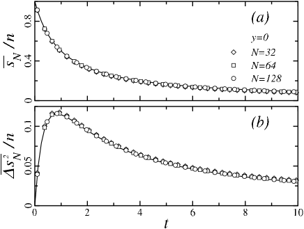
Figure 3: Scaling behaviour of (a) the mean value sN¯¯subscript𝑠𝑁\overline{s_{N}} and (b) the variance ΔsN2¯¯Δsuperscriptsubscript𝑠𝑁2\overline{\Delta s_{N}^{2}} of s=(sA+sB)/2𝑠subscript𝑠𝐴subscript𝑠𝐵2s=(s_{A}+s_{B})/2 as a function of the time t=k/N𝑡𝑘𝑁t=k/N. In the initial state ρA=ρB=1/2subscript𝜌𝐴subscript𝜌𝐵12\rho_{A}=\rho_{B}=1/2. The finite-size data for N=32𝑁32N=32 (diamond), 64 (square), 128 (circle) were deduced from SN(s,k)subscript𝑆𝑁𝑠𝑘S_{N}(s,k) given by a numerical iteration of the master equation (3.1). A good collapse on the full lines corresponding to the scaling functions in (3.17) and (3.18) is obtained. The variance is maximum for a number of updates k𝑘k close to N𝑁N.

Let us define the generating function

𝒮N(w,k)=s=dnswsSN(s,k)=r=dnr(nd)!(n+d)!(nr)!(n+r)!(12r2d2N2)kΩr,d(w)subscript𝒮𝑁𝑤𝑘superscriptsubscript𝑠𝑑𝑛𝑠superscript𝑤𝑠subscript𝑆𝑁𝑠𝑘superscriptsubscript𝑟𝑑𝑛𝑟𝑛𝑑𝑛𝑑𝑛𝑟𝑛𝑟superscript12superscript𝑟2superscript𝑑2superscript𝑁2𝑘subscriptΩ𝑟𝑑𝑤{\mathcal{S}}_{N}(w,k)=\sum_{s=d}^{n}sw^{s}S_{N}(s,k)=\sum_{r=d}^{n}\frac{r(n-d)!(n+d)!}{(n-r)!(n+r)!}\left(\!1\!-\!2\,\frac{r^{2}\!-\!d^{2}}{N^{2}}\right)^{k}\Omega_{r,d}(w) (3.11)

where

Ωr,d(w)=s=dr(1)rs(r+ssd)(r+ds+d)2swsr+s.subscriptΩ𝑟𝑑𝑤superscriptsubscript𝑠𝑑𝑟superscript1𝑟𝑠binomial𝑟𝑠𝑠𝑑binomial𝑟𝑑𝑠𝑑2𝑠superscript𝑤𝑠𝑟𝑠\Omega_{r,d}(w)=\sum_{s=d}^{r}(-1)^{r-s}{r+s\choose s-d}{r+d\choose s+d}\frac{2sw^{s}}{r+s}\,. (3.12)

In appendix B we show that when d=0𝑑0d=0

Ωr,0(1)=2subscriptΩ𝑟012\Omega_{r,0}(1)=2 (3.13)

and

dΩr,0dw|w=1=2r2,evaluated-at𝑑subscriptΩ𝑟0𝑑𝑤𝑤12superscript𝑟2\left.\frac{d\Omega_{r,0}}{dw}\right|_{w=1}=2r^{2}\,, (3.14)

which allows us to evaluate the mean value of s𝑠s

sN(k)¯=𝒮N(1,k)=r=1n2rj=1rnj+1n+j(12r2N2)k,d=0,formulae-sequence¯subscript𝑠𝑁𝑘subscript𝒮𝑁1𝑘superscriptsubscript𝑟1𝑛2𝑟superscriptsubscriptproduct𝑗1𝑟𝑛𝑗1𝑛𝑗superscript12superscript𝑟2superscript𝑁2𝑘𝑑0\overline{s_{N}(k)}={\mathcal{S}}_{N}(1,k)=\sum_{r=1}^{n}2r\prod_{j=1}^{r}\frac{n-j+1}{n+j}\left(\!1\!-\!2\,\frac{r^{2}}{N^{2}}\right)^{k}\,,\quad d=0\,, (3.15)

and its mean-square value:

sN2(k)¯=𝒮Nw|w=1=r=1n2r3j=1rnj+1n+j(12r2N2)k,d=0.formulae-sequence¯superscriptsubscript𝑠𝑁2𝑘evaluated-atsubscript𝒮𝑁𝑤𝑤1superscriptsubscript𝑟1𝑛2superscript𝑟3superscriptsubscriptproduct𝑗1𝑟𝑛𝑗1𝑛𝑗superscript12superscript𝑟2superscript𝑁2𝑘𝑑0\overline{s_{N}^{2}(k)}=\left.\frac{\partial{\mathcal{S}}_{N}}{\partial w}\right|_{w=1}\!\!\!\!\!=\sum_{r=1}^{n}2r^{3}\prod_{j=1}^{r}\frac{n-j+1}{n+j}\left(\!1\!-\!2\,\frac{r^{2}}{N^{2}}\right)^{k}\,,\quad d=0\,. (3.16)

In the scaling limit (N,n,k𝑁𝑛𝑘N,n,k\to\infty, t=k/N𝑡𝑘𝑁t=k/N) studied in appendix C, one obtains:

sN(t)¯n=s.l.1t+116n(11(t+1)3),sN2(t)¯n2=s.l.1(t+1)2t2n(t+1)4,d=0.\frac{\overline{s_{N}(t)}}{n}\stackrel{{\scriptstyle\mathrm{s.l.}}}{{=}}\frac{1}{t+1}-\frac{1}{6n}\left(1-\frac{1}{(t+1)^{3}}\right)\,,\quad\frac{\overline{s_{N}^{2}(t)}}{n^{2}}\stackrel{{\scriptstyle\mathrm{s.l.}}}{{=}}\frac{1}{(t+1)^{2}}-\frac{t}{2n(t+1)^{4}}\,,\quad d=0\,. (3.17)

In these expressions we kept the sub-leading contributions since the leading ones vanish in the variance given by:

ΔsN2(t)¯n=s.l.13(t+1)12(t+1)3+16(t+1)4,d=0.\frac{\overline{\Delta s_{N}^{2}(t)}}{n}\stackrel{{\scriptstyle\mathrm{s.l.}}}{{=}}\frac{1}{3(t+1)}-\frac{1}{2(t+1)^{3}}+\frac{1}{6(t+1)^{4}}\,,\qquad d=0\,. (3.18)

Thus the fluctuations are small and s𝑠s is self-averaging. A comparison with finite-size data is shown in figure 3. We were not able to evaluate Ωr,d(w)subscriptΩ𝑟𝑑𝑤\Omega_{r,d}(w) when d>0𝑑0d>0. This case is treated directly in the scaling limit in the next section.

3.5 Scaling limit when d0𝑑0d\geq 0
Refer to caption
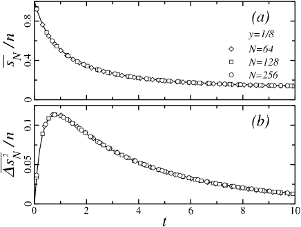
Figure 4: As in figure 3 for y=ρAρB=1/8𝑦subscript𝜌𝐴subscript𝜌𝐵18y=\rho_{A}-\rho_{B}=1/8 and N=64𝑁64N=64 (diamond), 128 (square), 256 (circle). The scaling functions (full lines) are given in (3.23) and (3.28).

Let us assume that in the scaling limit, for any value of d𝑑d, sN¯¯subscript𝑠𝑁\overline{s_{N}} and ΔsN2¯¯Δsuperscriptsubscript𝑠𝑁2\overline{\Delta s_{N}^{2}} are both growing as n𝑛n as in (3.17) and (3.18) for d=0𝑑0d=0. This suggests the introduction, besides the time variable t=k/(2n)𝑡𝑘2𝑛t=k/(2n) and the density y=d/n𝑦𝑑𝑛y=d/n, of the scaled and centered variable

σ(s,k)=ssN(k)¯n1/2.𝜎𝑠𝑘𝑠¯subscript𝑠𝑁𝑘superscript𝑛12\sigma(s,k)=\frac{s-\overline{s_{N}(k)}}{n^{1/2}}\,. (3.19)

Furthermore let us write the unknown mean value x¯¯𝑥\overline{x} as

x¯=sN¯n=gy(t),¯𝑥¯subscript𝑠𝑁𝑛subscript𝑔𝑦𝑡\overline{x}=\frac{\overline{s_{N}}}{n}=g_{y}(t)\,, (3.20)

and define the probability density:

𝔖(σ,t)=s.l.n1/2SN(s,k).{\mathfrak{S}}(\sigma,t)\stackrel{{\scriptstyle\mathrm{s.l.}}}{{=}}n^{1/2}S_{N}(s,k)\,. (3.21)

Starting from the master equation (3.1) with SNsubscript𝑆𝑁S_{N} replaced by 𝔖𝔖{\mathfrak{S}}, a Taylor expansion of the right-hand-side up to second order in s𝑠s and k𝑘k, when re-expressed in terms of the scaled variables, takes the form of an expansion in powers of n1/2superscript𝑛12n^{-1/2}. The terms independent of n𝑛n cancel. The terms of order n1/2superscript𝑛12n^{-1/2} leads to the differential equation

dgydt=(gy2y2),𝑑subscript𝑔𝑦𝑑𝑡superscriptsubscript𝑔𝑦2superscript𝑦2\frac{dg_{y}}{dt}=-(g_{y}^{2}-y^{2})\,, (3.22)

which is the mean-field equation (2.6) so that, according to (2.8),

x¯=gy(t)=y1+y+(1y)2yt1+y(1y)2yt,¯𝑥subscript𝑔𝑦𝑡𝑦1𝑦1𝑦superscript2𝑦𝑡1𝑦1𝑦superscript2𝑦𝑡\overline{x}=g_{y}(t)=y\,\frac{1+y+(1-y)\,\rme^{-2yt}}{1+y-(1-y)\,\rme^{-2yt}}\,, (3.23)

in agreement with (3.17) when y0𝑦0y\to 0. To the next order, n1superscript𝑛1n^{-1}, one obtains the following partial differential equation:

𝔖t=12[dgydt+12(dgydt)2]2𝔖σ2+2gy(𝔖+σ𝔖σ).𝔖𝑡12delimited-[]𝑑subscript𝑔𝑦𝑑𝑡12superscript𝑑subscript𝑔𝑦𝑑𝑡2superscript2𝔖superscript𝜎22subscript𝑔𝑦𝔖𝜎𝔖𝜎\frac{\partial{\mathfrak{S}}}{\partial t}=-\frac{1}{2}\left[\frac{dg_{y}}{dt}+\frac{1}{2}\left(\frac{dg_{y}}{dt}\right)^{2}\right]\frac{\partial^{2}{\mathfrak{S}}}{\partial\sigma^{2}}+2g_{y}\left({\mathfrak{S}}+\sigma\frac{\partial{\mathfrak{S}}}{\partial\sigma}\right)\,. (3.24)
Refer to caption
Figure 5: Data collapse for the scaled probability distribution n1/2SN(s,k)superscript𝑛12subscript𝑆𝑁𝑠𝑘n^{1/2}S_{N}(s,k) as a function of σ=n1/2(ssN(k)¯)𝜎superscript𝑛12𝑠¯subscript𝑠𝑁𝑘\sigma=n^{-1/2}(s-\overline{s_{N}(k)}) at different times t𝑡t and for increasing lattice sizes, N=256𝑁256N=256 (diamond), 512 (square) and 1024 (circle). In the initial state y=0 so that ρA=ρB=1/2subscript𝜌𝐴subscript𝜌𝐵12\rho_{A}=\rho_{B}=1/2. The finite-size data follow from a numerical iteration of the master equation (3.1). The full lines correspond to the Gaussian density (3.26) obtained in the scaling limit. The fluctuations are stronger for t1similar-to-or-equals𝑡1t\simeq 1.

Introducing the reduced variance κy(t)=ΔsN2¯/nsubscript𝜅𝑦𝑡¯Δsuperscriptsubscript𝑠𝑁2𝑛\kappa_{y}(t)=\overline{\Delta s_{N}^{2}}/n and assuming that 𝔖𝔖{\mathfrak{S}} depends on t𝑡t only through κysubscript𝜅𝑦\kappa_{y}, the partial differential equation (3.24) can be rewritten in the following form:

(𝔖κy122𝔖σ2)dκydt𝔖subscript𝜅𝑦12superscript2𝔖superscript𝜎2𝑑subscript𝜅𝑦𝑑𝑡\displaystyle\left(\frac{\partial{\mathfrak{S}}}{\partial\kappa_{y}}\!-\!\frac{1}{2}\frac{\partial^{2}{\mathfrak{S}}}{\partial\sigma^{2}}\right)\!\frac{d\kappa_{y}}{dt}\! =12[dκydt+4gyκy+dgydt+12(dgydt)2]2𝔖σ2absent12delimited-[]𝑑subscript𝜅𝑦𝑑𝑡4subscript𝑔𝑦subscript𝜅𝑦𝑑subscript𝑔𝑦𝑑𝑡12superscript𝑑subscript𝑔𝑦𝑑𝑡2superscript2𝔖superscript𝜎2\displaystyle=\!-\frac{1}{2}\!\left[\frac{d\kappa_{y}}{dt}\!+\!4g_{y}\kappa_{y}\!+\!\frac{dg_{y}}{dt}\!+\!\frac{1}{2}\left(\!\frac{dg_{y}}{dt}\!\right)^{2}\right]\!\frac{\partial^{2}{\mathfrak{S}}}{\partial\sigma^{2}} (3.25)
+2gy(𝔖+σ𝔖σ+κy2𝔖σ2).2subscript𝑔𝑦𝔖𝜎𝔖𝜎subscript𝜅𝑦superscript2𝔖superscript𝜎2\displaystyle\ \ \ \ \ \ \ \ \ \ \ \ \ \ \ \ \ \ \ \ \ \ \ \ \ \ \ \ \ \ \ \ \ \ \ \ \ \ \ +\!2g_{y}\!\left(\!{\mathfrak{S}}\!+\!\sigma\frac{\partial{\mathfrak{S}}}{\partial\sigma}\!+\!\kappa_{y}\frac{\partial^{2}{\mathfrak{S}}}{\partial\sigma^{2}}\right)\!\!.

The left-hand-side and the last bracket on the right-hand-side are both vanishing for the Gaussian density with variance κy(t)subscript𝜅𝑦𝑡\kappa_{y}(t), thus we have

𝔖(σ,t)=σ2/[2κy(t)]2πκy(t),𝔖𝜎𝑡superscriptsuperscript𝜎2delimited-[]2subscript𝜅𝑦𝑡2𝜋subscript𝜅𝑦𝑡{\mathfrak{S}}(\sigma,t)=\frac{\rme^{-\sigma^{2}/[2\kappa_{y}(t)]}}{\sqrt{2\pi\kappa_{y}(t)}}\,, (3.26)

when, according to (3.25), κy(t)subscript𝜅𝑦𝑡\kappa_{y}(t) satisfies the first-order differential equation:

dκydt+4gyκy+dgydt+12(dgydt)2=0.𝑑subscript𝜅𝑦𝑑𝑡4subscript𝑔𝑦subscript𝜅𝑦𝑑subscript𝑔𝑦𝑑𝑡12superscript𝑑subscript𝑔𝑦𝑑𝑡20\frac{d\kappa_{y}}{dt}+4g_{y}\kappa_{y}+\frac{dg_{y}}{dt}+\frac{1}{2}\left(\frac{dg_{y}}{dt}\right)^{2}=0\,. (3.27)

The solution is discussed in appendix D and reads:

κy(t)=s.l.ΔsN2¯n=[(1+y)22yt(1y)22yt4y(1+ty4t)]2y(1y2)4yt[1+y(1y)2yt]4.\kappa_{y}(t)\stackrel{{\scriptstyle\mathrm{s.l.}}}{{=}}\frac{\overline{\Delta s_{N}^{2}}}{n}=\left[(1\!+\!y)^{2}\rme^{2yt}\!-\!(1\!-\!y)^{2}\rme^{\!-\!2yt}\!-\!4y(1\!+\!t\!-\!y^{4}t)\right]\frac{2y(1\!-\!y^{2})\rme^{\!-\!4yt}}{\left[1\!+\!y\!-\!(1\!-\!y)\rme^{\!-\!2yt}\right]^{4}}\,. (3.28)

In the limit y0𝑦0y\to 0 (3.18) is recovered. The mean value in (3.23) and the variance are compared to finite-size data in figure 4.
Refer to caption
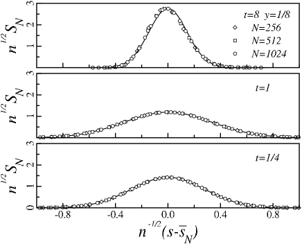
Figure 6: As in figure 5 for y=ρAρB=1/8𝑦subscript𝜌𝐴subscript𝜌𝐵18y=\rho_{A}-\rho_{B}=1/8.

The scaling behaviour of the probability distribution SN(s,k)subscript𝑆𝑁𝑠𝑘S_{N}(s,k) at different times is shown in figure 5 for ρA=ρBsubscript𝜌𝐴subscript𝜌𝐵\rho_{A}=\rho_{B} and figure 6 for ρAρB=1/8subscript𝜌𝐴subscript𝜌𝐵18\rho_{A}-\rho_{B}=1/8.

4 Time required to reach a given number of surviving particles

4.1 Probability distribution

This section is dedicated to the study of TN(s,k)subscript𝑇𝑁𝑠𝑘T_{N}(s,k), the probability distribution for the number of updates k𝑘k needed to reach for the first time a total number of surviving particles sA+sB=2ssubscript𝑠𝐴subscript𝑠𝐵2𝑠s_{A}+s_{B}=2s, as shown in figure 7(a). This probability is related to SN(s+1,k1)subscript𝑆𝑁𝑠1𝑘1S_{N}(s+1,k-1) through:

TN(s,k)=SN(s+1,k1)×2(s+1)2d2N2.subscript𝑇𝑁𝑠𝑘subscript𝑆𝑁𝑠1𝑘12superscript𝑠12superscript𝑑2superscript𝑁2T_{N}(s,k)=S_{N}(s+1,k-1)\times 2\frac{(s+1)^{2}-d^{2}}{N^{2}}\,. (4.1)

It is given by the product of the probability to be in a state with s=s+1superscript𝑠𝑠1s^{\prime}=s+1 after k1𝑘1k-1 updates by the probability of the transition s=s+1s′′=ssuperscript𝑠𝑠1superscript𝑠′′𝑠s^{\prime}=s+1\rightarrow~{}s^{\prime\prime}=s at the next update. Making use of (3.10) one obtains:

TN(s,k)=(nd)!(n+d)!n2(sd)!(s+d)!r=s+1n(1)rs1r(r+s)!(nr)!(n+r)!(rs1)!(12r2d2N2)k1.subscript𝑇𝑁𝑠𝑘𝑛𝑑𝑛𝑑superscript𝑛2𝑠𝑑𝑠𝑑superscriptsubscript𝑟𝑠1𝑛superscript1𝑟𝑠1𝑟𝑟𝑠𝑛𝑟𝑛𝑟𝑟𝑠1superscript12superscript𝑟2superscript𝑑2superscript𝑁2𝑘1T_{N}(s,k)=\frac{(n-d)!(n+d)!}{n^{2}(s-d)!(s+d)!}\sum_{r=s+1}^{n}\frac{(-1)^{r-s-1}r(r+s)!}{(n-r)!(n+r)!(r-s-1)!}\left(1\!-\!2\,\frac{r^{2}\!-\!d^{2}}{N^{2}}\right)^{k-1}\!\!\!\!\,. (4.2)

The evolution with k𝑘k is governed by the master equation

TN(s,k)=[12(s+1)2d2N2]TN(s,k1)+2(s+1)2d2N2TN(s+1,k1),subscript𝑇𝑁𝑠𝑘delimited-[]12superscript𝑠12superscript𝑑2superscript𝑁2subscript𝑇𝑁𝑠𝑘12superscript𝑠12superscript𝑑2superscript𝑁2subscript𝑇𝑁𝑠1𝑘1T_{N}(s,k)=\left[1-2\,\frac{(s+1)^{2}-d^{2}}{N^{2}}\right]\!T_{N}(s,k-1)+2\,\frac{(s+1)^{2}-d^{2}}{N^{2}}\,T_{N}(s+1,k-1)\,, (4.3)

which follows from (3.1) and (4.1).

4.2 Generating function

In order to calculate the mean value and the variance of the reaction time t=k/N𝑡𝑘𝑁t=k/N we introduce the generating function

𝒯N(s,z)=k=1zkTN(s,k).subscript𝒯𝑁𝑠𝑧superscriptsubscript𝑘1superscript𝑧𝑘subscript𝑇𝑁𝑠𝑘{\mathcal{T}}_{N}(s,z)=\sum_{k=1}^{\infty}z^{k}T_{N}(s,k)\,. (4.4)
Refer to caption
Figure 7: (a) Evolution of s=(sA+sB)/2superscript𝑠subscriptsuperscript𝑠𝐴subscriptsuperscript𝑠𝐵2s^{\prime}=(s^{\prime}_{A}+s^{\prime}_{B})/2 as a function of the number of updates k𝑘k. Initially all the sites are occupied, s=nsuperscript𝑠𝑛s^{\prime}=n. Small circles correspond to the final state of updates where ssuperscript𝑠s^{\prime} keeps the same value, bigger circles to a transition ss1superscript𝑠superscript𝑠1s^{\prime}\to s^{\prime}-1 when two particles annihilate. (b) Diagrams corresponding to the generating function N(s,z)subscript𝑁superscript𝑠𝑧{\mathcal{L}}_{N}(s^{\prime},z) in (4.5) for the lifetime of a state with 2s2superscript𝑠2s^{\prime} particles.

The evolution from s=nsuperscript𝑠𝑛s^{\prime}=n to s=ssuperscript𝑠𝑠s^{\prime}=s in figure 7(a) proceeds through a succession of steps where the system remains for some time in a state with sA+sB=2ssubscriptsuperscript𝑠𝐴subscriptsuperscript𝑠𝐵2superscript𝑠s^{\prime}_{A}+s^{\prime}_{B}=2s^{\prime} until two particles annihilate and ss1superscript𝑠superscript𝑠1s^{\prime}\rightarrow~{}s^{\prime}-1. We associate with such a step the generating function for its lifetime corresponding to the diagrams of figure 7(b):

N(s,z)subscript𝑁superscript𝑠𝑧\displaystyle{\mathcal{L}}_{N}(s^{\prime},z) ={1+z[12s2d2N2]++zl[12s2d2N2]llupdateswithoutannihilation+}2zs2d2N2annihilationabsent1𝑧delimited-[]12superscript𝑠2superscript𝑑2superscript𝑁2subscriptsuperscript𝑧𝑙superscriptdelimited-[]12superscript𝑠2superscript𝑑2superscript𝑁2𝑙𝑙updateswithoutannihilationsubscript2𝑧superscript𝑠2superscript𝑑2superscript𝑁2annihilation\displaystyle=\Bigg{\{}1+z\left[1-2\frac{s^{\prime 2}-d^{2}}{N^{2}}\right]+\cdots+\underbrace{z^{l}\left[1-2\frac{s^{\prime 2}-d^{2}}{N^{2}}\right]^{l}}_{l\ \mathrm{updates\ without\ annihilation}}+\cdots\Bigg{\}}\underbrace{2z\frac{s^{\prime 2}-d^{2}}{N^{2}}}_{\mathrm{annihilation}} (4.5)
=2z(s2d2)N2z[N22(s2d2)].absent2𝑧superscript𝑠2superscript𝑑2superscript𝑁2𝑧delimited-[]superscript𝑁22superscript𝑠2superscript𝑑2\displaystyle=\frac{2z(s^{\prime 2}-d^{2})}{N^{2}-z\left[N^{2}-2(s^{\prime 2}-d^{2})\right]}\,.

The generating function for the reaction time, measured in the number of updates, is obtained as the product:

𝒯N(s,z)=s=s+1nN(s,z)=(nd)!(n+d)!(sd)!(s+d)!(2z)nss=s+1n{N2z[N22(s2d2)]}.subscript𝒯𝑁𝑠𝑧superscriptsubscriptproductsuperscript𝑠𝑠1𝑛subscript𝑁superscript𝑠𝑧𝑛𝑑𝑛𝑑𝑠𝑑𝑠𝑑superscript2𝑧𝑛𝑠superscriptsubscriptproductsuperscript𝑠𝑠1𝑛superscript𝑁2𝑧delimited-[]superscript𝑁22superscript𝑠2superscript𝑑2{\mathcal{T}}_{N}(s,z)=\prod_{s^{\prime}=s+1}^{n}{\mathcal{L}}_{N}(s^{\prime},z)=\frac{(n-d)!(n+d)!}{(s-d)!(s+d)!}\,\frac{(2z)^{n-s}}{\prod_{s^{\prime}=s+1}^{n}\left\{N^{2}-z\left[N^{2}-2(s^{\prime 2}-d^{2})\right]\right\}}\,. (4.6)

It is easy to verify on this expression that 𝒯N(s,1)=k=1TN(s,k)=1subscript𝒯𝑁𝑠1superscriptsubscript𝑘1subscript𝑇𝑁𝑠𝑘1{\mathcal{T}}_{N}(s,1)=\sum_{k=1}^{\infty}T_{N}(s,k)=1 so that TN(s,k)subscript𝑇𝑁𝑠𝑘T_{N}(s,k) is properly normalized.

4.3 Mean value and variance

The mean value of the reaction time t=k/N𝑡𝑘𝑁t=k/N is given by:

tN(s)¯=1Nk=1kTN(s,k)=1N𝒯Nz|z=1=ns=s+1n1s2d2.¯subscript𝑡𝑁𝑠1𝑁superscriptsubscript𝑘1𝑘subscript𝑇𝑁𝑠𝑘evaluated-at1𝑁subscript𝒯𝑁𝑧𝑧1𝑛superscriptsubscriptsuperscript𝑠𝑠1𝑛1superscript𝑠2superscript𝑑2\overline{t_{N}(s)}=\frac{1}{N}\sum_{k=1}^{\infty}kT_{N}(s,k)=\frac{1}{N}\left.\frac{\partial{\mathcal{T}}_{N}}{\partial z}\right|_{z=1}=n\sum_{s^{\prime}=s+1}^{n}\frac{1}{s^{\prime 2}-d^{2}}\,. (4.7)

When d=0𝑑0d=0 one obtains

tN(s)¯=ns=s+1n1s2=n(Hn(2)Hs(2)),¯subscript𝑡𝑁𝑠𝑛superscriptsubscriptsuperscript𝑠𝑠1𝑛1superscript𝑠2𝑛superscriptsubscript𝐻𝑛2superscriptsubscript𝐻𝑠2\overline{t_{N}(s)}=n\sum_{s^{\prime}=s+1}^{n}\frac{1}{s^{\prime 2}}=n(H_{n}^{(2)}-H_{s}^{(2)})\,, (4.8)

where Hl(m)=j=1l1/jmsuperscriptsubscript𝐻𝑙𝑚superscriptsubscript𝑗1𝑙1superscript𝑗𝑚H_{l}^{(m)}=\sum_{j=1}^{l}1/j^{m} is a generalized harmonic number. When d>0𝑑0d>0 one may write

tN(s)¯=n2ds=s+1n(1sd1s+d)=n2d(HndHsdHn+d+Hs+d),¯subscript𝑡𝑁𝑠𝑛2𝑑superscriptsubscriptsuperscript𝑠𝑠1𝑛1superscript𝑠𝑑1superscript𝑠𝑑𝑛2𝑑subscript𝐻𝑛𝑑subscript𝐻𝑠𝑑subscript𝐻𝑛𝑑subscript𝐻𝑠𝑑\overline{t_{N}(s)}\!=\!\frac{n}{2d}\!\sum_{s^{\prime}=s+1}^{n}\!\left(\frac{1}{s^{\prime}\!-\!d}-\frac{1}{s^{\prime}\!+\!d}\right)\!=\frac{n}{2d}(H_{n-d}\!-\!H_{s-d}\!-\!H_{n+d}\!+\!H_{s+d})\,, (4.9)

where Hl=Hl(1)subscript𝐻𝑙superscriptsubscript𝐻𝑙1H_{l}=H_{l}^{(1)} is a harmonic number.

A second derivative gives the mean square value of the reaction time:

tN2(s)¯¯superscriptsubscript𝑡𝑁2𝑠\displaystyle\overline{t_{N}^{2}(s)} =1N2k=1k2TN(s,k)=1N2z(z𝒯Nz)|z=1absent1superscript𝑁2superscriptsubscript𝑘1superscript𝑘2subscript𝑇𝑁𝑠𝑘evaluated-at1superscript𝑁2𝑧𝑧subscript𝒯𝑁𝑧𝑧1\displaystyle=\frac{1}{N^{2}}\sum_{k=1}^{\infty}k^{2}T_{N}(s,k)=\frac{1}{N^{2}}\left.\frac{\partial}{\partial z}\left(z\frac{\partial{\mathcal{T}}_{N}}{\partial z}\right)\right|_{z=1} (4.10)
=n2(s=s+1n1s2d2)2+n2s=s+1n1(s2d2)212s=s+1n1s2d2.absentsuperscript𝑛2superscriptsuperscriptsubscriptsuperscript𝑠𝑠1𝑛1superscript𝑠2superscript𝑑22superscript𝑛2superscriptsubscriptsuperscript𝑠𝑠1𝑛1superscriptsuperscript𝑠2superscript𝑑2212superscriptsubscriptsuperscript𝑠𝑠1𝑛1superscript𝑠2superscript𝑑2\displaystyle=n^{2}\left(\sum_{s^{\prime}=s+1}^{n}\frac{1}{s^{\prime 2}\!-\!d^{2}}\!\right)^{2}\!\!\!+n^{2}\!\sum_{s^{\prime}=s+1}^{n}\frac{1}{(s^{\prime 2}\!-\!d^{2})^{2}}-\frac{1}{2}\!\sum_{s^{\prime}=s+1}^{n}\!\frac{1}{s^{\prime 2}\!-\!d^{2}}\,.

Since the first term in the last expression is tN(s)¯2superscript¯subscript𝑡𝑁𝑠2\overline{t_{N}(s)}^{2} the variance is given by:

ΔtN2(s)¯=n2s=v+1n1(s2d2)212s=s+1n1s2d2.¯Δsuperscriptsubscript𝑡𝑁2𝑠superscript𝑛2superscriptsubscriptsuperscript𝑠𝑣1𝑛1superscriptsuperscript𝑠2superscript𝑑2212superscriptsubscriptsuperscript𝑠𝑠1𝑛1superscript𝑠2superscript𝑑2\overline{\Delta t_{N}^{2}(s)}=n^{2}\!\sum_{s^{\prime}=v+1}^{n}\frac{1}{(s^{\prime 2}\!-\!d^{2})^{2}}-\frac{1}{2}\!\sum_{s^{\prime}=s+1}^{n}\!\frac{1}{s^{\prime 2}\!-\!d^{2}}\,. (4.11)

When d=0𝑑0d=0 one obtains:

ΔtN2(s)¯=n2s=s+1n1s412s=s+1n1s2=n2(Hn(4)Hs(4))12(Hn(2)Hs(2)).¯Δsuperscriptsubscript𝑡𝑁2𝑠superscript𝑛2superscriptsubscriptsuperscript𝑠𝑠1𝑛1superscript𝑠412superscriptsubscriptsuperscript𝑠𝑠1𝑛1superscript𝑠2superscript𝑛2superscriptsubscript𝐻𝑛4superscriptsubscript𝐻𝑠412superscriptsubscript𝐻𝑛2superscriptsubscript𝐻𝑠2\overline{\Delta t_{N}^{2}(s)}\!=\!n^{2}\!\sum_{s^{\prime}=s+1}^{n}\frac{1}{s^{\prime 4}}\!-\!\frac{1}{2}\!\sum_{s^{\prime}=s+1}^{n}\!\frac{1}{s^{\prime 2}}\!=\!n^{2}(H_{n}^{(4)}\!-\!H_{s}^{(4)})\!-\!\frac{1}{2}(H_{n}^{(2)}\!-\!H_{s}^{(2)})\,. (4.12)

When d>0𝑑0d>0 (4.11) can be rewritten as:

ΔtN2(s)¯¯Δsuperscriptsubscript𝑡𝑁2𝑠\displaystyle\overline{\Delta t_{N}^{2}(s)} =n24d2s=s+1n[1(sd)2+1(s+d)2]14d(1+n2d2)s=s+1n(1sd1s+d)absentsuperscript𝑛24superscript𝑑2superscriptsubscriptsuperscript𝑠𝑠1𝑛delimited-[]1superscriptsuperscript𝑠𝑑21superscriptsuperscript𝑠𝑑214𝑑1superscript𝑛2superscript𝑑2superscriptsubscriptsuperscript𝑠𝑠1𝑛1superscript𝑠𝑑1superscript𝑠𝑑\displaystyle=\frac{n^{2}}{4d^{2}}\sum_{s^{\prime}=s+1}^{n}\left[\frac{1}{(s^{\prime}-d)^{2}}+\frac{1}{(s^{\prime}+d)^{2}}\right]-\frac{1}{4d}\left(1+\frac{n^{2}}{d^{2}}\right)\sum_{s^{\prime}=s+1}^{n}\left(\frac{1}{s^{\prime}-d}-\frac{1}{s^{\prime}+d}\right) (4.13)
=n24d2(Hnd(2)Hsd(2)+Hn+d(2)Hs+d(2))14d(1+n2d2)(HndHsdHn+d+Hs+d).absentsuperscript𝑛24superscript𝑑2superscriptsubscript𝐻𝑛𝑑2superscriptsubscript𝐻𝑠𝑑2superscriptsubscript𝐻𝑛𝑑2superscriptsubscript𝐻𝑠𝑑214𝑑1superscript𝑛2superscript𝑑2subscript𝐻𝑛𝑑subscript𝐻𝑠𝑑subscript𝐻𝑛𝑑subscript𝐻𝑠𝑑\displaystyle=\!\frac{n^{2}}{4d^{2}}(H_{n\!-\!d}^{(2)}\!-\!H_{s\!-\!d}^{(2)}\!+\!H_{n\!+\!d}^{(2)}\!-\!H_{s\!+\!d}^{(2)})\!-\!\frac{1}{4d}\!\left(\!1\!+\!\frac{n^{2}}{d^{2}}\right)\!(H_{n\!-\!d}\!-\!H_{s\!-\!d}\!-\!H_{n\!\!+d}\!+\!H_{s\!+\!d})\,.

4.4 Scaling limit

In the scaling limit the probability distribution TN(s,k)subscript𝑇𝑁𝑠𝑘T_{N}(s,k) leads to three different probability densities, depending on the values of x=s/n𝑥𝑠𝑛x=s/n and y=d/n𝑦𝑑𝑛y=d/n. We now study these different cases.

4.4.1 x>y0𝑥𝑦0x>y\geq 0.

Refer to caption
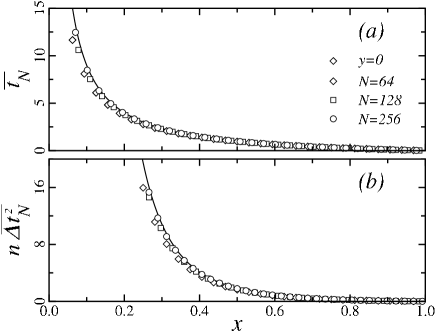
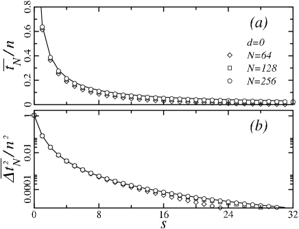
Figure 8: Scaling behaviour of (a) the mean value tN¯¯subscript𝑡𝑁\overline{t_{N}} and (b) the variance ΔtN2¯¯Δsuperscriptsubscript𝑡𝑁2\overline{\Delta t_{N}^{2}} of the time t𝑡t needed to reach a given value of x=ρA+ρB𝑥subscript𝜌𝐴subscript𝜌𝐵x=\rho_{A}+\rho_{B} with ρA=ρB=1/2subscript𝜌𝐴subscript𝜌𝐵12\rho_{A}=\rho_{B}=1/2 in the initial state. The finite-size data for N=64𝑁64N=64 (diamond), 128 (square), 256 (circle), given by (4.7) and (4.11), collapse on the full lines corresponding to the scaling functions in (4.16) and (4.19).
Refer to caption
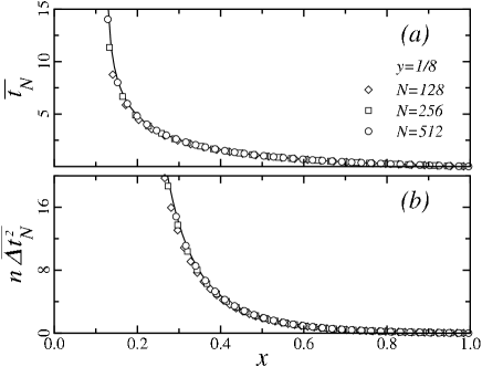
Figure 9: As in figure 8 for ρAρB=1/8subscript𝜌𝐴subscript𝜌𝐵18\rho_{A}-\rho_{B}=1/8 and N=128𝑁128N=128 (diamond), 256 (square), 512 (circle). The scaling functions are given in (4.15) and (4.18).

We first consider the case where both n,s,d𝑛𝑠𝑑n,s,d\to\infty for fixed values of the ratios x>y0𝑥𝑦0x>y\geq 0. Using in (4.9) the asymptotic expansion for harmonic numbers

Hnα=lnn+lnα+γ+O(n1),subscript𝐻𝑛𝛼𝑛𝛼𝛾Big-Osuperscript𝑛1H_{n\alpha}=\ln n+\ln\alpha+\gamma+\Or(n^{-1})\,, (4.14)

where γ𝛾\gamma is Euler’s constant, gives

tN¯=s.l.hy(x)=12yln[(1y)(x+y)(1+y)(xy)],\overline{t_{N}}\stackrel{{\scriptstyle\mathrm{s.l.}}}{{=}}h_{y}(x)=\frac{1}{2y}\ln\left[\frac{(1-y)(x+y)}{(1+y)(x-y)}\right]\,, (4.15)

which is the mean-field expression (2.11). It reduces to

tN¯=s.l.1x1,\overline{t_{N}}\stackrel{{\scriptstyle\mathrm{s.l.}}}{{=}}\frac{1}{x}-1\,, (4.16)

when y0𝑦0y\to 0.

Using the following expansion for generalized harmonic numbers

Hnβ(2)Hnα(2)=j=nα+1nβ1j2=nαnβdjj2+O(n2)=1n(1α1β)+O(n2)superscriptsubscript𝐻𝑛𝛽2superscriptsubscript𝐻𝑛𝛼2superscriptsubscript𝑗𝑛𝛼1𝑛𝛽1superscript𝑗2superscriptsubscript𝑛𝛼𝑛𝛽𝑑𝑗superscript𝑗2Big-Osuperscript𝑛21𝑛1𝛼1𝛽Big-Osuperscript𝑛2H_{n\beta}^{(2)}-H_{n\alpha}^{(2)}=\sum_{j=n\alpha+1}^{n\beta}\frac{1}{j^{2}}=\int_{n\alpha}^{n\beta}\frac{dj}{j^{2}}+\Or(n^{-2})=\frac{1}{n}\left(\frac{1}{\alpha}-\frac{1}{\beta}\right)+\Or(n^{-2}) (4.17)

as well as (4.14), the scaling limit of the variance follows from (4.13) and reads:

ΔtN2¯¯Δsuperscriptsubscript𝑡𝑁2\displaystyle\overline{\Delta t_{N}^{2}} =s.l.χy(x)n\displaystyle\stackrel{{\scriptstyle\mathrm{s.l.}}}{{=}}\frac{\chi_{y}(x)}{n}
χy(x)subscript𝜒𝑦𝑥\displaystyle\chi_{y}(x) =12y2(xx2y211y2)14y(1+1y2)ln[(1y)(x+y)(1+y)(xy)].absent12superscript𝑦2𝑥superscript𝑥2superscript𝑦211superscript𝑦214𝑦11superscript𝑦21𝑦𝑥𝑦1𝑦𝑥𝑦\displaystyle=\frac{1}{2y^{2}}\!\left(\frac{x}{x^{2}\!-\!y^{2}}-\frac{1}{1\!-\!y^{2}}\right)\!-\!\frac{1}{4y}\left(1\!+\!\frac{1}{y^{2}}\right)\ln\left[\frac{(1\!-\!y)(x\!+\!y)}{(1\!+\!y)(x\!-\!y)}\right]\,. (4.18)

When y0𝑦0y\to 0 one obtains:

χ0(x)=13x312x+16.subscript𝜒0𝑥13superscript𝑥312𝑥16\chi_{0}(x)=\frac{1}{3x^{3}}-\frac{1}{2x}+\frac{1}{6}\,. (4.19)

Here too the fluctuations are small and t𝑡t is a self-averaging variable when x>y𝑥𝑦x>y.

The dependence on x=ρA+ρB𝑥subscript𝜌𝐴subscript𝜌𝐵x=\rho_{A}+\rho_{B} of the mean value and the variance of the reaction time t𝑡t is shown in figure 8 for y=ρAρB=0𝑦subscript𝜌𝐴subscript𝜌𝐵0y=\rho_{A}-\rho_{B}=0 and figure 9 for y=1/8𝑦18y=1/8. A good collapse of the finite-size data is obtained.
Refer to caption
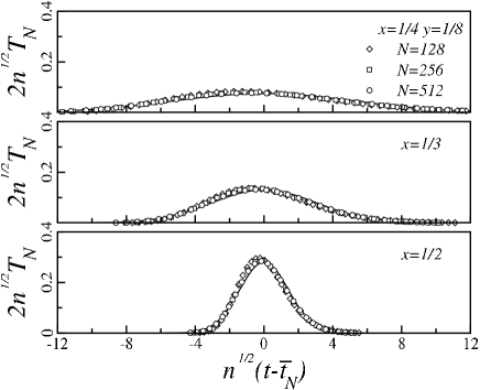
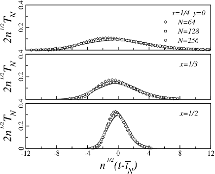
Figure 10: Data collapse for the scaled probability distribution 2n1/2TN(s,k)2superscript𝑛12subscript𝑇𝑁𝑠𝑘2n^{1/2}T_{N}(s,k) as a function of θ=n1/2(ttN(s)¯)𝜃superscript𝑛12𝑡¯subscript𝑡𝑁𝑠\theta=n^{1/2}(t-\overline{t_{N}(s)}) at different values of the particle density x=ρA+ρB𝑥subscript𝜌𝐴subscript𝜌𝐵x=\rho_{A}+\rho_{B} and for increasing lattice sizes, N=64𝑁64N=64 (diamond), 128 (square) and 256 (circle). In the initial state ρA=ρB=1/2subscript𝜌𝐴subscript𝜌𝐵12\rho_{A}=\rho_{B}=1/2. The full lines correspond to the Gaussian density, 𝔗(x,θ)𝔗𝑥𝜃{\mathfrak{T}}(x,\theta) in (4.24), which is obtained in the scaling limit. The fluctuations are growing as x𝑥x decreases.
Refer to caption
Figure 11: As in figure 10 for y=ρAρB=1/8𝑦subscript𝜌𝐴subscript𝜌𝐵18y=\rho_{A}-\rho_{B}=1/8 with N=128𝑁128N=128 (diamond), 256 (square), 512 (circle).

The scaling of the variance with n𝑛n suggests the definition of the following scale-invariant and centered time variable

θ(s,k)=n1/2(ttN¯),t=k2nformulae-sequence𝜃𝑠𝑘superscript𝑛12𝑡¯subscript𝑡𝑁𝑡𝑘2𝑛\theta(s,k)=n^{1/2}(t-\overline{t_{N}})\,,\qquad t=\frac{k}{2n} (4.20)

where tN¯¯subscript𝑡𝑁\overline{t_{N}} given by (4.15) depends on s𝑠s through x=s/n𝑥𝑠𝑛x=s/n. Accordingly we define the probability density as:

𝔗(x,θ)=s.l.2n1/2TN(s,k).{\mathfrak{T}}(x,\theta)\stackrel{{\scriptstyle\mathrm{s.l.}}}{{=}}2n^{1/2}T_{N}(s,k)\,. (4.21)

We proceed as in section 3.5 222Except that here the expression of tN¯¯subscript𝑡𝑁\overline{t_{N}} is already known. and solve the master equation (4.3) in the scaling limit.
Refer to caption
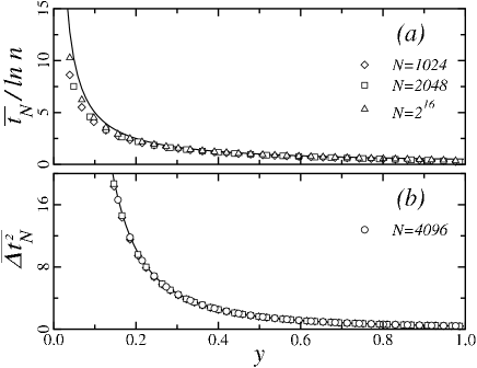
Figure 12: Scaling behaviour of (a) the mean value tN¯¯subscript𝑡𝑁\overline{t_{N}} and (b) the variance ΔtN2¯¯Δsuperscriptsubscript𝑡𝑁2\overline{\Delta t_{N}^{2}} of the time t𝑡t needed to reach a state with y=x=ρA𝑦𝑥subscript𝜌𝐴y=x=\rho_{A} and u=ρB=0𝑢subscript𝜌𝐵0u=\rho_{B}=0 with ρA=(1+y)/2subscript𝜌𝐴1𝑦2\rho_{A}=(1+y)/2 and ρB=(1y)/2subscript𝜌𝐵1𝑦2\rho_{B}=(1-y)/2 in the initial state. The finite-size data for N=1024𝑁1024N=1024 (diamond), 2048 (square), 4096 (circle), 216superscript2162^{16} (triangle), given by (4.7) and (4.11), collapse on the full lines corresponding to the scaling functions in (4.26) and (4.27). The convergence is slow for tN¯¯subscript𝑡𝑁\overline{t_{N}} due to a correction to scaling of order (lnn)1superscript𝑛1(\ln n)^{-1}.

We replace TNsubscript𝑇𝑁T_{N} by 𝔗𝔗{\mathfrak{T}}, make a Taylor expansion of 𝔗𝔗{\mathfrak{T}} to second order in s𝑠s and k𝑘k and rewrite the coefficients and the derivatives in terms of the new scaled variables. In this way an expansion in powers of n1/2superscript𝑛12n^{-1/2} is obtained. The coefficients of n0superscript𝑛0n^{0} and n1/2superscript𝑛12n^{-1/2} vanish identically. The first non-vanishing contribution is coming at order n1superscript𝑛1n^{-1} and leads to the partial differential equation:

𝔗x=12(x2y2)(121x2y2)2𝔗θ2.𝔗𝑥12superscript𝑥2superscript𝑦2121superscript𝑥2superscript𝑦2superscript2𝔗superscript𝜃2\frac{\partial{\mathfrak{T}}}{\partial x}=\frac{1}{2(x^{2}-y^{2})}\left(\frac{1}{2}-\frac{1}{x^{2}-y^{2}}\right)\frac{\partial^{2}{\mathfrak{T}}}{\partial\theta^{2}}\,. (4.22)

Assuming that 𝔗𝔗{\mathfrak{T}} depends on x𝑥x only through the reduced variance χy(x)subscript𝜒𝑦𝑥\chi_{y}(x) given by (4.18) the partial differential equation transforms into the diffusion equation

𝔗χy=122𝔗θ2.𝔗subscript𝜒𝑦12superscript2𝔗superscript𝜃2\frac{\partial{\mathfrak{T}}}{\partial\chi_{y}}=\frac{1}{2}\frac{\partial^{2}{\mathfrak{T}}}{\partial\theta^{2}}\,. (4.23)

Thus the fluctuations are Gaussian:

𝔗(x,θ)=θ2/[2χy(x)]2πχy(x),x>y0.formulae-sequence𝔗𝑥𝜃superscriptsuperscript𝜃2delimited-[]2subscript𝜒𝑦𝑥2𝜋subscript𝜒𝑦𝑥𝑥𝑦0{\mathfrak{T}}(x,\theta)=\frac{\rme^{-\theta^{2}/[2\chi_{y}(x)]}}{\sqrt{2\pi\chi_{y}(x)}}\,,\qquad x>y\geq 0\,. (4.24)

The Gaussian behaviour of the reaction time is shown for different values of x=ρA+ρB𝑥subscript𝜌𝐴subscript𝜌𝐵x=\rho_{A}+\rho_{B} in figure 10 for ρA=ρBsubscript𝜌𝐴subscript𝜌𝐵\rho_{A}=\rho_{B} and figure 11 for ρAρB=1/8subscript𝜌𝐴subscript𝜌𝐵18\rho_{A}-\rho_{B}=1/8. The finite-size results were obtained by iterating the master equation (3.1), storing the data at each update for a given value of s=nx+1𝑠𝑛𝑥1s=nx+1 and using (4.1).

4.4.2 x=y>0𝑥𝑦0x=y>0, sd𝑠𝑑s\geq d.

We study now the case where s=d+u𝑠𝑑𝑢s=d+u with d=ny𝑑𝑛𝑦d=ny, sA=O(n)subscript𝑠𝐴Big-O𝑛s_{A}=\Or(n) and sB=u=O(1)subscript𝑠𝐵𝑢Big-O1s_{B}=u=\Or(1), i.e. when the reaction is close to completion or complete. The mean reaction time which follows from (4.9)

tN¯=12y[ln(2ny1y1+y)+γHu]+O(n1),¯subscript𝑡𝑁12𝑦delimited-[]2𝑛𝑦1𝑦1𝑦𝛾subscript𝐻𝑢Big-Osuperscript𝑛1\overline{t_{N}}=\frac{1}{2y}\left[\ln\left(2ny\frac{1-y}{1+y}\right)+\gamma-H_{u}\right]+\Or(n^{-1})\,, (4.25)

has a slow logarithmic growth with n𝑛n which in the scaling limit yields:

tN¯lnn=12y+O[(lnn)]1).\frac{\overline{t_{N}}}{\ln n}=\frac{1}{2y}+\Or[(\ln n)]^{-1})\,. (4.26)

The variance in (4.13) gives

ΔtN2¯=14y2[ζ(2)Hu(2)]+O(lnnn).¯Δsuperscriptsubscript𝑡𝑁214superscript𝑦2delimited-[]𝜁2superscriptsubscript𝐻𝑢2Big-O𝑛𝑛\overline{\Delta t_{N}^{2}}=\frac{1}{4y^{2}}\left[\zeta(2)-H_{u}^{(2)}\right]+\Or\left(\frac{\ln n}{n}\right)\,. (4.27)

The fluctuations of the reaction time t𝑡t are stronger when the reaction is completed or close to completion. The finite-size data collapse for the mean value and the variance as a function of y𝑦y is shown in figure 12.

In this regime the ratio ΔtN2¯/tN¯¯Δsuperscriptsubscript𝑡𝑁2¯subscript𝑡𝑁\sqrt{\overline{\Delta t_{N}^{2}}}/\overline{t_{N}} decreases slowly as (lnn)1superscript𝑛1(\ln n)^{-1} which suggests a new type of statistics. It will be obtained by taking the scaling limit directly on the probability distribution TN(s,k)subscript𝑇𝑁𝑠𝑘T_{N}(s,k) in (4.2). Since the variance does not depend on n𝑛n we define a centered time variable as:

θ=2y(ttN¯),t=k2n.formulae-sequencesuperscript𝜃2𝑦𝑡¯subscript𝑡𝑁𝑡𝑘2𝑛\theta^{\prime}=2y(t-\overline{t_{N}})\,,\qquad t=\frac{k}{2n}\,. (4.28)

The factor 2y2𝑦2y is suggested by the form of tN¯¯subscript𝑡𝑁\overline{t_{N}} given by (4.25). With this definition one obtains:

k=ny[θ+ln(2ny1y1+y)+γHu].𝑘𝑛𝑦delimited-[]superscript𝜃2𝑛𝑦1𝑦1𝑦𝛾subscript𝐻𝑢k=\frac{n}{y}\left[\theta^{\prime}+\ln\left(2ny\frac{1-y}{1+y}\right)+\gamma-H_{u}\right]\,. (4.29)

Thus one defines the probability density as:

𝔗(u,θ)=s.l.nyTN(d+u,k).{\mathfrak{T}}^{\prime}(u,\theta^{\prime})\stackrel{{\scriptstyle\mathrm{s.l.}}}{{=}}\frac{n}{y}T_{N}(d+u,k)\,. (4.30)

With the change of summation variable r=j+d+u+1𝑟𝑗𝑑𝑢1r=j+d+u+1 (4.2) leads to

nyTN(d+u,k)=1u!j=0ndu1(1)jj!AjBjCjDj(1Ej)k1,𝑛𝑦subscript𝑇𝑁𝑑𝑢𝑘1𝑢superscriptsubscript𝑗0𝑛𝑑𝑢1superscript1𝑗𝑗subscript𝐴𝑗subscript𝐵𝑗subscript𝐶𝑗subscript𝐷𝑗superscript1subscript𝐸𝑗𝑘1\frac{n}{y}T_{N}(d+u,k)=\frac{1}{u!}\sum_{j=0}^{n-d-u-1}\frac{(-1)^{j}}{j!}A_{j}B_{j}C_{j}D_{j}\left(1-E_{j}\right)^{k-1}\,, (4.31)

where, in the scaling limit with d=ny𝑑𝑛𝑦d=ny:

Aj=d+j+u+1d=1+j+u+1ny1,subscript𝐴𝑗𝑑𝑗𝑢1𝑑1𝑗𝑢1𝑛𝑦similar-to-or-equals1A_{j}=\frac{d+j+u+1}{d}=1+\frac{j+u+1}{ny}\simeq 1\,, (4.32)
Bj=(nd)!(ndju1)!=i=0j+u(ndi)(nd)j+u+1,subscript𝐵𝑗𝑛𝑑𝑛𝑑𝑗𝑢1superscriptsubscriptproduct𝑖0𝑗𝑢𝑛𝑑𝑖similar-to-or-equalssuperscript𝑛𝑑𝑗𝑢1B_{j}=\frac{(n\!-\!d)!}{(n\!-\!d\!-\!j\!-\!u\!-\!1)!}=\prod_{i=0}^{j+u}(n-d-i)\simeq(n\!-\!d)^{j+u+1}\,, (4.33)
Cj=(n+d)!(n+d+j+u+1)!=[i=1j+u+1(n+d+i)]1(n+d)(j+u+1),subscript𝐶𝑗𝑛𝑑𝑛𝑑𝑗𝑢1superscriptdelimited-[]superscriptsubscriptproduct𝑖1𝑗𝑢1𝑛𝑑𝑖1similar-to-or-equalssuperscript𝑛𝑑𝑗𝑢1C_{j}=\frac{(n\!+\!d)!}{(n\!+\!d\!+\!j\!+\!u\!+\!1)!}=\left[\prod_{i=1}^{j+u+1}(n+d+i)\right]^{-1}\simeq(n\!+\!d)^{-(j+u+1)}\,, (4.34)
Dj=(2d+2u+j+1)!(2d+u)!=i=1j+u+1(2d+u+i)(2d)j+u+1,subscript𝐷𝑗2𝑑2𝑢𝑗12𝑑𝑢superscriptsubscriptproduct𝑖1𝑗𝑢12𝑑𝑢𝑖similar-to-or-equalssuperscript2𝑑𝑗𝑢1D_{j}=\frac{(2d\!+\!2u\!+\!j\!+\!1)!}{(2d\!+\!u)!}=\prod_{i=1}^{j+u+1}(2d+u+i)\simeq(2d)^{j+u+1}\,, (4.35)
Ej=(d+j+u+1)2d22n2=2d+j+u+12n2(j+u+1)yn(j+u+1).subscript𝐸𝑗superscript𝑑𝑗𝑢12superscript𝑑22superscript𝑛22𝑑𝑗𝑢12superscript𝑛2𝑗𝑢1similar-to-or-equals𝑦𝑛𝑗𝑢1E_{j}=\frac{(d\!+\!j\!+\!u\!+\!1)^{2}-d^{2}}{2n^{2}}=\frac{2d\!+\!j\!+\!u\!+\!1}{2n^{2}}\,(j\!+\!u\!+\!1)\simeq\frac{y}{n}\,(j\!+\!u\!+\!1)\,. (4.36)
Refer to caption
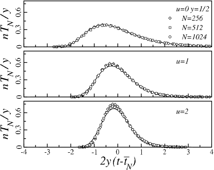
Figure 13: Data collapse for the scaled probability distribution nTN(s,k)/y𝑛subscript𝑇𝑁𝑠𝑘𝑦nT_{N}(s,k)/y as a function of θ=2y(ttN(s)¯)superscript𝜃2𝑦𝑡¯subscript𝑡𝑁𝑠\theta^{\prime}=2y(t-\overline{t_{N}(s)}) at different values of u=sB𝑢subscript𝑠𝐵u=s_{B}, for y=ρAρB=1/2𝑦subscript𝜌𝐴subscript𝜌𝐵12y=\rho_{A}-\rho_{B}=1/2 and increasing lattice sizes, N=256𝑁256N=256 (diamond), 512 (square) and 1024 (circle). The full lines correspond to the generalized Gumbel distribution in (4.39), which crosses over to a Gaussian as u𝑢u increases.

Taking into account the expression of k𝑘k in (4.29) one obtains:

(1Ej)k1(2ny1y1+y)(j+u+1)(j+u+1)(θ+γHu)similar-to-or-equalssuperscript1subscript𝐸𝑗𝑘1superscript2𝑛𝑦1𝑦1𝑦𝑗𝑢1superscript𝑗𝑢1superscript𝜃𝛾subscript𝐻𝑢\left(1-E_{j}\right)^{k-1}\simeq\left(2ny\frac{1-y}{1+y}\right)^{-(j+u+1)}\rme^{-(j+u+1)(\theta^{\prime}+\gamma-H_{u})} (4.37)

Thus in the scaling limit (4.31) gives

𝔗(u,θ)=1u!(u+1)(θ+γHuj=0[(θ+γHu]jj!,{\mathfrak{T}}^{\prime}(u,\theta^{\prime})=\frac{1}{u!}\rme^{-(u+1)(\theta^{\prime}+\gamma-H_{u}}\sum_{j=0}^{\infty}\frac{\left[-\rme^{-(\theta^{\prime}+\gamma-H_{u}}\right]^{j}}{j!}\,, (4.38)

which is the generalized Gumbel distribution [29, 30]:

𝔗(u,θ)=1u!exp[(u+1)(θ+γHu)(θ+γHu)].superscript𝔗𝑢superscript𝜃1𝑢𝑢1superscript𝜃𝛾subscript𝐻𝑢superscriptsuperscript𝜃𝛾subscript𝐻𝑢{\mathfrak{T}}^{\prime}(u,\theta^{\prime})=\frac{1}{u!}\exp\left[-(u+1)(\theta^{\prime}+\gamma-H_{u})-\rme^{-(\theta^{\prime}+\gamma-H_{u})}\right]\,. (4.39)

It crosses over to the Gaussian in (4.24) when u1much-greater-than𝑢1u\gg 1. The matching of the two probability densities is studied in appendix E. The collapse of the finite-size data on the generalized Gumbel distribution is shown in figure 13 for different values of u𝑢u and y=ρAρB=1/2𝑦subscript𝜌𝐴subscript𝜌𝐵12y=\rho_{A}-\rho_{B}=1/2. The finite-size data were obtained by iterating (3.1) and using (4.1).

4.4.3 x=y=0𝑥𝑦0x=y=0, sd𝑠𝑑s\geq d.

Refer to caption
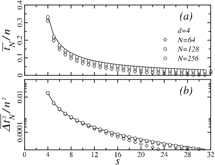
Figure 14: Scaling behaviour of (a) the mean value tN¯¯subscript𝑡𝑁\overline{t_{N}} and (b) the variance ΔtN2¯¯Δsuperscriptsubscript𝑡𝑁2\overline{\Delta t_{N}^{2}} of the time t𝑡t needed to reach a given value of s=(sA+sB)/2𝑠subscript𝑠𝐴subscript𝑠𝐵2s=(s_{A}+s_{B})/2 with sA=sB=nsubscript𝑠𝐴subscript𝑠𝐵𝑛s_{A}=s_{B}=n in the initial state. The finite-size data for N=64𝑁64N=64 (diamond), 128 (square), 256 (circle), given by (4.7) and (4.11), given by (4.7) and (4.11), collapse on the full lines corresponding to the scaling functions in (4.40).
Refer to caption
Figure 15: As in figure 14 with sA=n+4subscript𝑠𝐴𝑛4s_{A}=n+4 and sB=n4subscript𝑠𝐵𝑛4s_{B}=n-4 in the initial state. The scaling functions are now given by (4.41).

Finally we consider the case when s=O(1)d𝑠Big-O1𝑑s=\Or(1)\geq d. According to (4.8) and (4.12) in the scaling limit the mean value and the variance of the reaction time behave as

tN¯n=s.l.ζ(2)Hs(2),ΔtN2¯n2=s.l.ζ(4)Hs(4),\frac{\overline{t_{N}}}{n}\stackrel{{\scriptstyle\mathrm{s.l.}}}{{=}}\zeta(2)-H_{s}^{(2)}\,,\qquad\frac{\overline{\Delta t_{N}^{2}}}{n^{2}}\stackrel{{\scriptstyle\mathrm{s.l.}}}{{=}}\zeta(4)-H_{s}^{(4)}\,, (4.40)

when d=0𝑑0d=0 whereas (4.9) and (4.13) lead to

tN¯n=s.l.12d(Hs+dHsd),ΔtN2¯n2=s.l.14d2[2ζ(2)Hsd(2)Hs+d(2)+1d(HsdHs+d)],\frac{\overline{t_{N}}}{n}\stackrel{{\scriptstyle\mathrm{s.l.}}}{{=}}\frac{1}{2d}(H_{s+d}-H_{s-d})\,,\quad\frac{\overline{\Delta t_{N}^{2}}}{n^{2}}\stackrel{{\scriptstyle\mathrm{s.l.}}}{{=}}\frac{1}{4d^{2}}\left[2\zeta(2)\!-\!H_{s-d}^{(2)}\!-\!H_{s+d}^{(2)}\!+\!\frac{1}{d}(H_{s-d}\!-\!H_{s+d})\right], (4.41)

when d>0𝑑0d>0. The finite-size data collapse is shown in figure 14 for sA=sBsubscript𝑠𝐴subscript𝑠𝐵s_{A}=s_{B} and figure 15 for d=(sAsB)/2=4𝑑subscript𝑠𝐴subscript𝑠𝐵24d=(s_{A}-s_{B})/2=4.

The mean value and the standard deviation are both growing as n𝑛n, thus the reaction time is a strongly fluctuating random variable when the reaction is almost complete. In the following we use the scale-invariant time variable

θ′′=tn=k2n2,superscript𝜃′′𝑡𝑛𝑘2superscript𝑛2\theta^{\prime\prime}=\frac{t}{n}=\frac{k}{2n^{2}}\,, (4.42)

and define the associated probability density as:

𝔗′′(s,θ′′)=s.l.2n2TN(s,k).{\mathfrak{T}}^{\prime\prime}(s,\theta^{\prime\prime})\stackrel{{\scriptstyle\mathrm{s.l.}}}{{=}}2n^{2}T_{N}(s,k)\,. (4.43)
Refer to caption
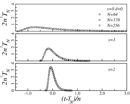
Figure 16: Data collapse for the scaled probability distribution 2n2TN(s,k)2superscript𝑛2subscript𝑇𝑁𝑠𝑘2n^{2}T_{N}(s,k) as a function of θ′′θ′′¯=(ttN(s)¯)/nsuperscript𝜃′′¯superscript𝜃′′𝑡¯subscript𝑡𝑁𝑠𝑛\theta^{\prime\prime}-\overline{\theta^{\prime\prime}}=(t-\overline{t_{N}(s)})/n at different values of s=(sA+sB)/2𝑠subscript𝑠𝐴subscript𝑠𝐵2s=(s_{A}+s_{B})/2, for sA=sB=nsubscript𝑠𝐴subscript𝑠𝐵𝑛s_{A}=s_{B}=n in the initial state and increasing lattice sizes, N=64𝑁64N=64 (diamond), 128 (square) and 256 (circle). The full lines correspond to the probability density 𝔗′′(s,θ′′θ′′¯)superscript𝔗′′𝑠superscript𝜃′′¯superscript𝜃′′{\mathfrak{T}}^{\prime\prime}(s,\theta^{\prime\prime}-\overline{\theta^{\prime\prime}}) in (4.46), which crosses over to a Gaussian as s𝑠s increases.
Refer to caption
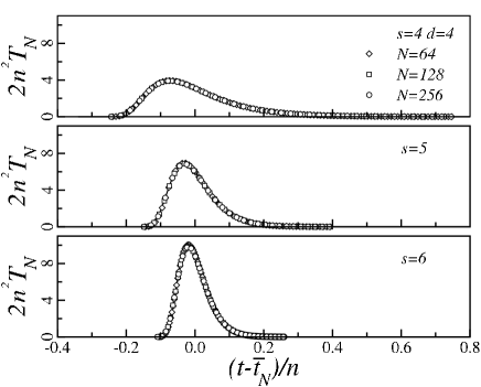
Figure 17: As in figure 16 with sA=n+4subscript𝑠𝐴𝑛4s_{A}=n+4 and sB=n4subscript𝑠𝐵𝑛4s_{B}=n-4 in the initial state.

In the expression (4.2) of TN(s,k)subscript𝑇𝑁𝑠𝑘T_{N}(s,k) one may write:

r(r+s)!(rs1)!=(1)s+1m=0s(m2r2).𝑟𝑟𝑠𝑟𝑠1superscript1𝑠1superscriptsubscriptproduct𝑚0𝑠superscript𝑚2superscript𝑟2\frac{r(r+s)!}{(r-s-1)!}=(-1)^{s+1}\prod_{m=0}^{s}(m^{2}-r^{2})\,. (4.44)

Furthermore, in the scaling limit, one obtains:

(12r2d2N2)k1(r2d2)θ′′,(nd)!(n+d)!(nr)!(n+r)!=j=dr1njn+j+11.formulae-sequencesimilar-to-or-equalssuperscript12superscript𝑟2superscript𝑑2superscript𝑁2𝑘1superscriptsuperscript𝑟2superscript𝑑2superscript𝜃′′𝑛𝑑𝑛𝑑𝑛𝑟𝑛𝑟superscriptsubscriptproduct𝑗𝑑𝑟1𝑛𝑗𝑛𝑗1similar-to-or-equals1\left(1-2\frac{r^{2}-d^{2}}{N^{2}}\right)^{k-1}\simeq\rme^{-(r^{2}-d^{2})\theta^{\prime\prime}}\,,\qquad\frac{(n-d)!(n+d)!}{(n-r)!(n+r)!}=\prod_{j=d}^{r-1}\frac{n-j}{n+j+1}\simeq 1\,. (4.45)

Thus the probability density is given by:

𝔗′′(s,θ′′)=2d2θ′′(sd)!(s+d)!r=s+1(1)rm=0s(m2r2)r2θ′′.superscript𝔗′′𝑠superscript𝜃′′2superscriptsuperscript𝑑2superscript𝜃′′𝑠𝑑𝑠𝑑superscriptsubscript𝑟𝑠1superscript1𝑟superscriptsubscriptproduct𝑚0𝑠superscript𝑚2superscript𝑟2superscriptsuperscript𝑟2superscript𝜃′′{\mathfrak{T}}^{\prime\prime}(s,\theta^{\prime\prime})=\frac{2\,\rme^{d^{2}\theta^{\prime\prime}}}{(s-d)!(s+d)!}\sum_{r=s+1}^{\infty}(-1)^{r}\prod_{m=0}^{s}(m^{2}-r^{2})\,\rme^{-r^{2}\theta^{\prime\prime}}\,. (4.46)
\psfrag{Y}[Bc][Bc][1][1]{$\mathfrak{T}^{\prime\prime}(s,\theta^{\prime\prime})$}\psfrag{X}[tc][tc][1][0]{$\theta^{\prime\prime}$}\psfrag{a}[Bc][Bc][1][1]{\tiny$s=0$}\psfrag{b}[Bc][Bc][1][1]{\tiny$s=1$}\psfrag{c}[Bc][Bc][1][1]{\tiny$s=2$}\psfrag{d}[Bc][Bc][1][1]{\tiny$d=0$}\includegraphics[width=227.62204pt,angle={0}]{fig-18.eps}
Figure 18: Semi-logarithmic plot of 𝔗(s,θ′′)𝔗𝑠superscript𝜃′′{\mathfrak{T}}(s,\theta^{\prime\prime}) in (4.46) for s=0,1,2𝑠012s=0,1,2 with sA=sB=nsubscript𝑠𝐴subscript𝑠𝐵𝑛s_{A}=s_{B}=n in the initial state. The dashed lines correspond to the asymptotic behaviour in (4.47) for θ′′1much-less-thansuperscript𝜃′′1\theta^{\prime\prime}\ll 1 and (4.53) for θ′′1much-greater-thansuperscript𝜃′′1\theta^{\prime\prime}\gg 1. A similar agreement is obtained when d>0𝑑0d>0.

The collapse of the finite-size data on 𝔗′′(s,θ′′)superscript𝔗′′𝑠superscript𝜃′′{\mathfrak{T}}^{\prime\prime}(s,\theta^{\prime\prime}) is shown at different values of s𝑠s for sA=sBsubscript𝑠𝐴subscript𝑠𝐵s_{A}=s_{B} in figure 16 and for d=(sAsB)/2=4𝑑subscript𝑠𝐴subscript𝑠𝐵24d=(s_{A}-s_{B})/2=4 in figure 17. The finite-size data were obtained by iterating (3.1) and using (4.1).

The asymptotic behaviour for θ′′1much-greater-thansuperscript𝜃′′1\theta^{\prime\prime}\gg 1 (see figure 18) is governed by the first term in the sum and reads:

𝔗′′(s,θ′′)2(s+1)(2s+1)(2ss+d)[(s+1)2d2]θ′′,θ′′1.formulae-sequencesimilar-to-or-equalssuperscript𝔗′′𝑠superscript𝜃′′2𝑠12𝑠1binomial2𝑠𝑠𝑑superscriptdelimited-[]superscript𝑠12superscript𝑑2superscript𝜃′′much-greater-thansuperscript𝜃′′1{\mathfrak{T}}^{\prime\prime}(s,\theta^{\prime\prime})\simeq 2(s+1)(2s+1){2s\choose s+d}\rme^{-[(s+1)^{2}-d^{2}]\theta^{\prime\prime}}\,,\qquad\theta^{\prime\prime}\gg 1\,. (4.47)

In order to study the asymptotic behaviour when θ′′1much-less-thansuperscript𝜃′′1\theta^{\prime\prime}\ll 1 it will be convenient to re-express 𝔗′′(s,θ′′)superscript𝔗′′𝑠superscript𝜃′′{\mathfrak{T}}^{\prime\prime}(s,\theta^{\prime\prime}) in terms of Jacobi theta functions. First let us notice that the product in (4.46) vanishes for rs𝑟𝑠r\leq s so that the sum can start at r=1𝑟1r=1 instead of s+1𝑠1s+1. The product can then be replaced by the differential operator m=0s(m2+d/dθ′′)superscriptsubscriptproduct𝑚0𝑠superscript𝑚2𝑑𝑑superscript𝜃′′\prod_{m=0}^{s}(m^{2}+d/d\theta^{\prime\prime}) so that:

r=s+1(1)rm=0s(m2r2)r2θ′′=m=0s(m2+d/dθ′′)r=1(1)rr2θ′′.superscriptsubscript𝑟𝑠1superscript1𝑟superscriptsubscriptproduct𝑚0𝑠superscript𝑚2superscript𝑟2superscriptsuperscript𝑟2superscript𝜃′′superscriptsubscriptproduct𝑚0𝑠superscript𝑚2𝑑𝑑superscript𝜃′′superscriptsubscript𝑟1superscript1𝑟superscriptsuperscript𝑟2superscript𝜃′′\sum_{r=s+1}^{\infty}(-1)^{r}\prod_{m=0}^{s}(m^{2}-r^{2})\,\rme^{-r^{2}\theta^{\prime\prime}}=\prod_{m=0}^{s}(m^{2}+d/d\theta^{\prime\prime})\sum_{r=1}^{\infty}(-1)^{r}\rme^{-r^{2}\theta^{\prime\prime}}\,. (4.48)

Making use of the identity ([33] p 463)

r=1(1)rqr2cos(2rz)=ϑ4(z,q)12,superscriptsubscript𝑟1superscript1𝑟superscript𝑞superscript𝑟22𝑟𝑧subscriptitalic-ϑ4𝑧𝑞12\sum_{r=1}^{\infty}(-1)^{r}q^{r^{2}}\cos(2rz)=\frac{\vartheta_{4}(z,q)-1}{2}\,, (4.49)

one obtains

𝔗′′(s,θ′′)=d2θ′′(sd)!(s+d)!m=0s(m2+d/dθ′′)ϑ4(0,θ′′),superscript𝔗′′𝑠superscript𝜃′′superscriptsuperscript𝑑2superscript𝜃′′𝑠𝑑𝑠𝑑superscriptsubscriptproduct𝑚0𝑠superscript𝑚2𝑑𝑑superscript𝜃′′subscriptitalic-ϑ40superscriptsuperscript𝜃′′{\mathfrak{T}}^{\prime\prime}(s,\theta^{\prime\prime})=\frac{\rme^{d^{2}\theta^{\prime\prime}}}{(s-d)!(s+d)!}\prod_{m=0}^{s}(m^{2}+d/d\theta^{\prime\prime})\,\vartheta_{4}\left(0,\rme^{-\theta^{\prime\prime}}\right)\,, (4.50)

where the Jacobi theta function can be re-written as ([33] p 475):

ϑ4(0,θ′′)=πθ′′ϑ2(0,π2/θ′′)=2πθ′′r=0(r+1/2)2π2/θ′′.subscriptitalic-ϑ40superscriptsuperscript𝜃′′𝜋superscript𝜃′′subscriptitalic-ϑ20superscriptsuperscript𝜋2superscript𝜃′′2𝜋superscript𝜃′′superscriptsubscript𝑟0superscriptsuperscript𝑟122superscript𝜋2superscript𝜃′′\vartheta_{4}\left(0,\rme^{-\theta^{\prime\prime}}\right)=\sqrt{\frac{\pi}{\theta^{\prime\prime}}}\vartheta_{2}\left(0,\rme^{-\pi^{2}/\theta^{\prime\prime}}\right)=2\sqrt{\frac{\pi}{\theta^{\prime\prime}}}\sum_{r=0}^{\infty}\rme^{-(r+1/2)^{2}\pi^{2}/\theta^{\prime\prime}}\,. (4.51)

Finally the probability density takes the following form:

𝔗′′(s,θ′′)=2d2θ′′(sd)!(s+d)!m=0s(m2+d/dθ′′)πθ′′r=0(r+1/2)2π2/θ′′.superscript𝔗′′𝑠superscript𝜃′′2superscriptsuperscript𝑑2superscript𝜃′′𝑠𝑑𝑠𝑑superscriptsubscriptproduct𝑚0𝑠superscript𝑚2𝑑𝑑superscript𝜃′′𝜋superscript𝜃′′superscriptsubscript𝑟0superscriptsuperscript𝑟122superscript𝜋2superscript𝜃′′{\mathfrak{T}}^{\prime\prime}(s,\theta^{\prime\prime})=\frac{2\rme^{d^{2}\theta^{\prime\prime}}}{(s\!-\!d)!(s\!+\!d)!}\prod_{m=0}^{s}(m^{2}\!+\!d/d\theta^{\prime\prime})\sqrt{\frac{\pi}{\theta^{\prime\prime}}}\sum_{r=0}^{\infty}\rme^{-(r+1/2)^{2}\pi^{2}/\theta^{\prime\prime}}\!\!. (4.52)

The leading contribution when θ′′1much-less-thansuperscript𝜃′′1\theta^{\prime\prime}\ll 1 (see figure 18) comes from the derivatives of the exponential in the first term of the sum so that:

𝔗′′(s,θ′′)22(sd)!(s+d)!(π2θ′′)2s+5/2π2/(4θ′′),θ′′1.formulae-sequencesimilar-to-or-equalssuperscript𝔗′′𝑠superscript𝜃′′22𝑠𝑑𝑠𝑑superscript𝜋2superscript𝜃′′2𝑠52superscriptsuperscript𝜋24superscript𝜃′′much-less-thansuperscript𝜃′′1{\mathfrak{T}}^{\prime\prime}(s,\theta^{\prime\prime})\simeq\frac{2\sqrt{2}}{(s\!-\!d)!(s\!+\!d)!}\left(\frac{\pi}{2\theta^{\prime\prime}}\right)^{2s+5/2}\rme^{-\pi^{2}/(4\theta^{\prime\prime})}\,,\qquad\theta^{\prime\prime}\ll 1\,. (4.53)

5 Conclusion

The two-species diffusion-annihilation process A+B𝐴𝐵absentA+B\rightarrow Ø  has been studied on the fully-connected lattice with size N𝑁N for either equal or different numbers of particles, sAsubscript𝑠𝐴s_{A} and sBsubscript𝑠𝐵s_{B}, in the initial state where sA+sB=N=2nsubscript𝑠𝐴subscript𝑠𝐵𝑁2𝑛s_{A}+s_{B}=N=2n. Exact probability distributions, SNsubscript𝑆𝑁S_{N} for s=(sA+sB)/2𝑠subscript𝑠𝐴subscript𝑠𝐵2s=(s_{A}+s_{B})/2 at a given time and TNsubscript𝑇𝑁T_{N} for the reaction time t𝑡t needed to reach a given number of surviving particles, have been obtained by solving the master equation. The finite-size scaling behaviour of the mean value and the variance of s𝑠s and t𝑡t has been determined using a generating function approach.

In the scaling limit, the fluctuations of the number of particles around their mean values, given exactly by mean-field theory, are weak and Gaussian. The statistical properties of the reaction time display three different regimes. When both sAsubscript𝑠𝐴s_{A} and sBsubscript𝑠𝐵s_{B} are O(n)Big-O𝑛\Or(n) the fluctuations of the reaction time, as measured by the ratio R=ΔtN2¯/tN¯𝑅¯Δsuperscriptsubscript𝑡𝑁2¯subscript𝑡𝑁R=\sqrt{\overline{\Delta t_{N}^{2}}}/\overline{t_{N}}, decay as n1/2superscript𝑛12n^{-1/2}. The fluctuations are Gaussian and mean-field theory is exact. For unequal initial densities, in the vicinity of the absorbing state when sA=O(n)subscript𝑠𝐴Big-O𝑛s_{A}=\Or(n) and sB=O(1)subscript𝑠𝐵Big-O1s_{B}=\Or(1), one obtains R=O[(lnn)1]𝑅Big-Osuperscript𝑛1R=\Or[(\ln n)^{-1}] thus the fluctuations are “marginally weak”. They are governed by a generalized Gumbel distribution, indexed by sBsubscript𝑠𝐵s_{B}, which crosses over to the Gaussian density with increasing values of sBsubscript𝑠𝐵s_{B}. For equal or almost equal initial numbers of particles and when the system is close to the absorbing state, i.e. when sA=O(1)sB0subscript𝑠𝐴Big-O1subscript𝑠𝐵0s_{A}=\Or(1)\geq s_{B}\geq 0, one obtains R=O(1)𝑅Big-O1R=\Or(1). The reaction time is then strongly fluctuating. Its probability density involves an alternating infinite series which can be considered as resulting from the applications of a product of s+1𝑠1s+1 first-order differential operators to a Jacobi theta function.

A generalized Gumbel distribution has been recently shown to govern the fluctuations of the covering time of the fully-connected lattice, i.e. the time needed for a random walker to visit almost each site at least once [34] (see also [35]). Although the two problems present some analogies (they share the same value of R𝑅R and the same probability density), the mean values and the variances scale differently with N𝑁N, the number of random walkers is constant for the covering time and decreasing for the reaction time.

The extreme value statistics obtained for the reaction time near the absorbing state, for almost equal initial numbers of A𝐴A and B𝐵B particles, is quite similar to what was obtained in [28] for the coagulation process A+AA𝐴𝐴𝐴A+A\rightarrow\ A. Probability densities with nearly the same form of asymptotics govern the behaviour of the squared width of an interface generated by a periodic Brownian motion [36] as well as the maximum height of the 1D Edwards-Wilkinson model [37, 38, 39, 40, 41].

It seems reasonable to conjecture that similar extreme value statistics should govern the reaction time when the system is close to its absorbing state for D>Dc=2𝐷subscript𝐷c2D>D_{\mathrm{c}}=2 when sAsB=O(n)subscript𝑠𝐴subscript𝑠𝐵Big-O𝑛s_{A}-s_{B}=\Or(n) in the initial state and for D>Dseg=4𝐷subscript𝐷seg4D>D_{\mathrm{seg}}=4 when sAsB=O(1)subscript𝑠𝐴subscript𝑠𝐵Big-O1s_{A}-s_{B}=\Or(1) in the initial state.

Appendix A Evaluation of 𝒗𝒓(𝒓)superscriptsubscript𝒗𝒓𝒓v_{r}^{(r)}

According to (3.6), in the initial state:

SN(n,0)=1=vn(n).subscript𝑆𝑁𝑛01superscriptsubscript𝑣𝑛𝑛S_{N}(n,0)=1=v_{n}^{(n)}\,. (1.1)

The recursion relation (3.5) gives

SN(n1,0)=0=vn1(n1)+vn1(n)=vn1(n1)n2d2n2(n1)2,subscript𝑆𝑁𝑛100superscriptsubscript𝑣𝑛1𝑛1superscriptsubscript𝑣𝑛1𝑛superscriptsubscript𝑣𝑛1𝑛1superscript𝑛2superscript𝑑2superscript𝑛2superscript𝑛12S_{N}(n-1,0)=0=v_{n-1}^{(n-1)}+v_{n-1}^{(n)}=v_{n-1}^{(n-1)}-\frac{n^{2}-d^{2}}{n^{2}-(n-1)^{2}}\,, (1.2)

so that:

vn1(n1)=n2d2n2(n1)2.superscriptsubscript𝑣𝑛1𝑛1superscript𝑛2superscript𝑑2superscript𝑛2superscript𝑛12v_{n-1}^{(n-1)}=\frac{n^{2}-d^{2}}{n^{2}-(n-1)^{2}}\,. (1.3)

In the same way

SN(n2,0)=0=vn2(n2)+vn2(n1)+vn2(n)subscript𝑆𝑁𝑛200superscriptsubscript𝑣𝑛2𝑛2superscriptsubscript𝑣𝑛2𝑛1superscriptsubscript𝑣𝑛2𝑛S_{N}(n-2,0)=0=v_{n-2}^{(n-2)}+v_{n-2}^{(n-1)}+v_{n-2}^{(n)} (1.4)

where

vn2(n1)superscriptsubscript𝑣𝑛2𝑛1\displaystyle v_{n-2}^{(n-1)} =(n1)2d2(n1)2(n2)2vn1(n1)=(n2d2)[(n1)2d2][n2(n1)2][(n1)2(n2)2],absentsuperscript𝑛12superscript𝑑2superscript𝑛12superscript𝑛22superscriptsubscript𝑣𝑛1𝑛1superscript𝑛2superscript𝑑2delimited-[]superscript𝑛12superscript𝑑2delimited-[]superscript𝑛2superscript𝑛12delimited-[]superscript𝑛12superscript𝑛22\displaystyle=-\frac{(n-1)^{2}-d^{2}}{(n-1)^{2}-(n-2)^{2}}v_{n-1}^{(n-1)}=-\frac{(n^{2}-d^{2})[(n-1)^{2}-d^{2}]}{[n^{2}-(n-1)^{2}][(n-1)^{2}-(n-2)^{2}]}\,,
vn2(n)superscriptsubscript𝑣𝑛2𝑛\displaystyle v_{n-2}^{(n)} =(n1)2d2n2(n2)2vn1(n)=(n2d2)[(n1)2d2][n2(n1)2][n2(n2)2],absentsuperscript𝑛12superscript𝑑2superscript𝑛2superscript𝑛22superscriptsubscript𝑣𝑛1𝑛superscript𝑛2superscript𝑑2delimited-[]superscript𝑛12superscript𝑑2delimited-[]superscript𝑛2superscript𝑛12delimited-[]superscript𝑛2superscript𝑛22\displaystyle=-\frac{(n-1)^{2}-d^{2}}{n^{2}-(n-2)^{2}}v_{n-1}^{(n)}=\frac{(n^{2}-d^{2})[(n-1)^{2}-d^{2}]}{[n^{2}-(n-1)^{2}][n^{2}-(n-2)^{2}]}\,, (1.5)

so that:

vn2(n2)=(n2d2)[(n1)2d2][n2(n2)2][(n1)2(n2)2].superscriptsubscript𝑣𝑛2𝑛2superscript𝑛2superscript𝑑2delimited-[]superscript𝑛12superscript𝑑2delimited-[]superscript𝑛2superscript𝑛22delimited-[]superscript𝑛12superscript𝑛22v_{n-2}^{(n-2)}=\frac{(n^{2}-d^{2})[(n-1)^{2}-d^{2}]}{[n^{2}-(n-2)^{2}][(n-1)^{2}-(n-2)^{2}]}\,. (1.6)

After lengthy but straitforward calculations the same procedure leads to:

vn3(n3)=(n2d2)[(n1)2d2][(n2)2d2][n2(n3)2][(n1)2(n3)2][(n2)2(n3)2].superscriptsubscript𝑣𝑛3𝑛3superscript𝑛2superscript𝑑2delimited-[]superscript𝑛12superscript𝑑2delimited-[]superscript𝑛22superscript𝑑2delimited-[]superscript𝑛2superscript𝑛32delimited-[]superscript𝑛12superscript𝑛32delimited-[]superscript𝑛22superscript𝑛32v_{n-3}^{(n-3)}=\frac{(n^{2}-d^{2})[(n-1)^{2}-d^{2}][(n-2)^{2}-d^{2}]}{[n^{2}-(n-3)^{2}][(n-1)^{2}-(n-3)^{2}][(n-2)^{2}-(n-3)^{2}]}\,. (1.7)

These results suggest the following conjecture

vr(r)=j=0nr1(nj)2d2(nj)2r2,r=d,,n1,vn(n)=1,formulae-sequencesuperscriptsubscript𝑣𝑟𝑟superscriptsubscriptproduct𝑗0𝑛𝑟1superscript𝑛𝑗2superscript𝑑2superscript𝑛𝑗2superscript𝑟2formulae-sequence𝑟𝑑𝑛1superscriptsubscript𝑣𝑛𝑛1v_{r}^{(r)}=\prod_{j=0}^{n-r-1}\frac{(n-j)^{2}-d^{2}}{(n-j)^{2}-r^{2}}\,,\qquad r=d,\ldots,n-1\,,\qquad v_{n}^{(n)}=1\,, (1.8)

from which (3.7) can be deduced.

Appendix B Calculation of 𝛀𝒓,𝟎(𝒘)subscript𝛀𝒓0𝒘\Omega_{r,0}(w) and its first derivative at 𝒘=𝟏𝒘1w=1

According to (3.12) when d=0𝑑0d=0

Ωr,0(w)=s=0r(1)rs(r+ss)(rs)2swsr+s.subscriptΩ𝑟0𝑤superscriptsubscript𝑠0𝑟superscript1𝑟𝑠binomial𝑟𝑠𝑠binomial𝑟𝑠2𝑠superscript𝑤𝑠𝑟𝑠\Omega_{r,0}(w)=\sum_{s=0}^{r}(-1)^{r-s}{r+s\choose s}{r\choose s}\frac{2sw^{s}}{r+s}\,. (2.1)

Using the following combinatorial identity for Legendre polynomials [31]

Pr(2w1)=s=0r(1)rs(r+ss)(rs)wssubscript𝑃𝑟2𝑤1superscriptsubscript𝑠0𝑟superscript1𝑟𝑠binomial𝑟𝑠𝑠binomial𝑟𝑠superscript𝑤𝑠P_{r}(2w-1)=\sum_{s=0}^{r}(-1)^{r-s}{r+s\choose s}{r\choose s}w^{s} (2.2)

(2.1) can be rewritten as:

Ωr,0(w)=2wr0wdPr(2u1)duur𝑑u.subscriptΩ𝑟0𝑤2superscript𝑤𝑟superscriptsubscript0𝑤𝑑subscript𝑃𝑟2𝑢1𝑑𝑢superscript𝑢𝑟differential-d𝑢\Omega_{r,0}(w)=2w^{-r}\!\int_{0}^{w}\frac{dP_{r}(2u-1)}{du}u^{r}du\,. (2.3)

An integration by parts gives:

Ωr,0(w)=2Pr(2w1)2rwr0wPr(2u1)ur1𝑑u.subscriptΩ𝑟0𝑤2subscript𝑃𝑟2𝑤12𝑟superscript𝑤𝑟superscriptsubscript0𝑤subscript𝑃𝑟2𝑢1superscript𝑢𝑟1differential-d𝑢\Omega_{r,0}(w)=2P_{r}(2w-1)-2rw^{-r}\int_{0}^{w}P_{r}(2u-1)u^{r-1}du\,. (2.4)

When w=1𝑤1w=1 one has:

Ωr,0(1)=22r01Pr(2u1)ur1𝑑u=2r11(x+12)r1Pr(x)𝑑x.subscriptΩ𝑟0122𝑟superscriptsubscript01subscript𝑃𝑟2𝑢1superscript𝑢𝑟1differential-d𝑢2𝑟superscriptsubscript11superscript𝑥12𝑟1subscript𝑃𝑟𝑥differential-d𝑥\Omega_{r,0}(1)=2-2r\!\int_{0}^{1}P_{r}(2u-1)\,u^{r-1}du=2-r\!\int_{-1}^{1}\left(\frac{x+1}{2}\right)^{r-1}\!\!\!\!P_{r}(x)dx\,. (2.5)

According to the identity [32]

11(1+x)σPν(x)𝑑x=2σ+1[Γ(σ+1)]2Γ(σ+ν+2)Γ(σν+1),superscriptsubscript11superscript1𝑥𝜎subscript𝑃𝜈𝑥differential-d𝑥superscript2𝜎1superscriptdelimited-[]Γ𝜎12Γ𝜎𝜈2Γ𝜎𝜈1\int_{-1}^{1}(1+x)^{\sigma}P_{\nu}(x)dx=\frac{2^{\sigma+1}\left[\Gamma(\sigma+1)\right]^{2}}{\Gamma(\sigma+\nu+2)\Gamma(\sigma-\nu+1)}\,, (2.6)

the integral in (2.5) vanishes and (3.13) is obtained.

The first derivative of (2.4) at w=1𝑤1w=1 gives:

dΩr,0dw|w=1=2dPr(2w1)dw|w=12revaluated-at𝑑subscriptΩ𝑟0𝑑𝑤𝑤1evaluated-at2𝑑subscript𝑃𝑟2𝑤1𝑑𝑤𝑤12𝑟\left.\frac{d\Omega_{r,0}}{dw}\right|_{w=1}=2\left.\frac{dP_{r}(2w-1)}{dw}\right|_{w=1}-2r (2.7)

The generating function for Legendre polynomials

l=0Pl(x)ul=112ux+u2superscriptsubscript𝑙0subscript𝑃𝑙𝑥superscript𝑢𝑙112𝑢𝑥superscript𝑢2\sum_{l=0}^{\infty}P_{l}(x)u^{l}=\frac{1}{\sqrt{1-2ux+u^{2}}} (2.8)

leads to:

l=0dPl(x)dx|x=1ul=u(1u)3=j=0(j+22)uj+1.evaluated-atsuperscriptsubscript𝑙0𝑑subscript𝑃𝑙𝑥𝑑𝑥𝑥1superscript𝑢𝑙𝑢superscript1𝑢3superscriptsubscript𝑗0binomial𝑗22superscript𝑢𝑗1\sum_{l=0}^{\infty}\left.\frac{dP_{l}(x)}{dx}\right|_{x=1}u^{l}=\frac{u}{(1-u)^{3}}=\sum_{j=0}^{\infty}{j+2\choose 2}u^{j+1}\,. (2.9)

Identifying the coefficients of ursuperscript𝑢𝑟u^{r}, one obtains

dPr(2w1)dw|w=1=2(r+12)=r(r+1),evaluated-at𝑑subscript𝑃𝑟2𝑤1𝑑𝑤𝑤12binomial𝑟12𝑟𝑟1\left.\frac{dP_{r}(2w-1)}{dw}\right|_{w=1}\!\!\!=2\,{r+1\choose 2}=r(r+1)\,, (2.10)

and (2.7) leads to (3.14).

Appendix C Scaling limit of 𝒔𝑵¯/𝒏bold-¯subscript𝒔𝑵𝒏\overline{s_{N}}/n and 𝒔𝑵𝟐¯/𝒏𝟐bold-¯superscriptsubscript𝒔𝑵2superscript𝒏2\overline{s_{N}^{2}}/n^{2} when 𝒅=𝟎𝒅0d=0

According to (3.15) one may write:

sN(k)¯n=r=1nf(r),f(r)=2rnrj=1rnjn+jp(r)(12r2N2)kek(r).formulae-sequence¯subscript𝑠𝑁𝑘𝑛superscriptsubscript𝑟1𝑛𝑓𝑟𝑓𝑟2𝑟𝑛𝑟subscriptsuperscriptsubscriptproduct𝑗1𝑟𝑛𝑗𝑛𝑗𝑝𝑟subscriptsuperscript12superscript𝑟2superscript𝑁2𝑘subscript𝑒𝑘𝑟\frac{\overline{s_{N}(k)}}{n}=\sum_{r=1}^{n}f(r)\,,\qquad f(r)=\frac{2r}{n-r}\underbrace{\prod_{j=1}^{r}\frac{n-j}{n+j}}_{p(r)}\,\,\underbrace{\left(\!1\!-\!2\,\frac{r^{2}}{N^{2}}\right)^{k}}_{e_{k}(r)}\,. (3.1)

Making use of the following expansions in powers of n1superscript𝑛1n^{-1}

2rnr2rn(1+rn+r2n2),similar-to-or-equals2𝑟𝑛𝑟2𝑟𝑛1𝑟𝑛superscript𝑟2superscript𝑛2\frac{2r}{n-r}\simeq\frac{2r}{n}\left(1+\frac{r}{n}+\frac{r^{2}}{n^{2}}\right)\,, (3.2)
lnp(r)𝑝𝑟\displaystyle\ln p(r) =j=1r[ln(1jn)ln(1+jn)]2j=1r(jn+j33n3)absentsuperscriptsubscript𝑗1𝑟delimited-[]1𝑗𝑛1𝑗𝑛similar-to-or-equals2superscriptsubscript𝑗1𝑟𝑗𝑛superscript𝑗33superscript𝑛3\displaystyle=\sum_{j=1}^{r}\left[\ln\left(1-\frac{j}{n}\right)-\ln\left(1+\frac{j}{n}\right)\right]\simeq-2\sum_{j=1}^{r}\left(\frac{j}{n}+\frac{j^{3}}{3n^{3}}\right) (3.3)
r(r+1)nr2(r+1)26n3,similar-to-or-equalsabsent𝑟𝑟1𝑛superscript𝑟2superscript𝑟126superscript𝑛3\displaystyle\simeq-\frac{r(r+1)}{n}-\frac{r^{2}(r+1)^{2}}{6n^{3}}\,,
lnek(r)=kln(12r2N2)2k(r2N2+r4N4)t(r2n+r44n3),subscript𝑒𝑘𝑟𝑘12superscript𝑟2superscript𝑁2similar-to-or-equals2𝑘superscript𝑟2superscript𝑁2superscript𝑟4superscript𝑁4similar-to-or-equals𝑡superscript𝑟2𝑛superscript𝑟44superscript𝑛3\ln e_{k}(r)=k\ln\left(1-2\frac{r^{2}}{N^{2}}\right)\simeq-2k\left(\frac{r^{2}}{N^{2}}+\frac{r^{4}}{N^{4}}\right)\simeq-t\left(\frac{r^{2}}{n}+\frac{r^{4}}{4n^{3}}\right), (3.4)

one obtains:

f(r)=2rn(1+rn+r2n2)exp[(t+1)r2nrnr2(r+1)26n3tr44n3].𝑓𝑟2𝑟𝑛1𝑟𝑛superscript𝑟2superscript𝑛2𝑡1superscript𝑟2𝑛𝑟𝑛superscript𝑟2superscript𝑟126superscript𝑛3𝑡superscript𝑟44superscript𝑛3f(r)\!=\!\frac{2r}{n}\left(1\!+\!\frac{r}{n}\!+\!\frac{r^{2}}{n^{2}}\right)\exp\left[-(t\!+\!1)\frac{r^{2}}{n}\!-\!\frac{r}{n}\!-\!\frac{r^{2}(r\!+\!1)^{2}}{6n^{3}}-\frac{tr^{4}}{4n^{3}}\right]\,. (3.5)

In the scaling limit the Euler-Maclaurin summation formula gives

r=1nf(r)0f(r)𝑑r+12[f()f(0)]+112[f()f(0)]+,similar-to-or-equalssuperscriptsubscript𝑟1𝑛𝑓𝑟superscriptsubscript0𝑓𝑟differential-d𝑟12delimited-[]𝑓𝑓0112delimited-[]superscript𝑓superscript𝑓0\sum_{r=1}^{n}f(r)\simeq\!\int_{0}^{\infty}\!\!f(r)\,dr\!+\!\frac{1}{2}\,[f(\infty)-f(0)]\!+\!\frac{1}{12}\,[f^{\prime}(\infty)-f^{\prime}(0)]+\ldots\,, (3.6)

with

f(0)=f()=f()=0,f(0)=2n.formulae-sequence𝑓0𝑓superscript𝑓0superscript𝑓02𝑛f(0)=f(\infty)=f^{\prime}(\infty)=0\,,\qquad f^{\prime}(0)=\frac{2}{n}\,. (3.7)

With the change of variable u=r2/n𝑢superscript𝑟2𝑛u=r^{2}/n (3.5) and (3.6) lead to:

r=1nf(r)superscriptsubscript𝑟1𝑛𝑓𝑟\displaystyle\sum_{r=1}^{n}f(r) 0𝑑u(1+un+un)(1unu26ntu24n+u2n)(t+1)u16nsimilar-to-or-equalsabsentsuperscriptsubscript0differential-d𝑢1𝑢𝑛𝑢𝑛1𝑢𝑛superscript𝑢26𝑛𝑡superscript𝑢24𝑛𝑢2𝑛superscript𝑡1𝑢16𝑛\displaystyle\simeq\int_{0}^{\infty}\!\!du\left(1\!+\!\sqrt{\frac{u}{n}}\!+\!\frac{u}{n}\right)\left(1\!-\!\sqrt{\frac{u}{n}}\!-\!\frac{u^{2}}{6n}\!-\!\frac{tu^{2}}{4n}+\!\frac{u}{2n}\right)\rme^{-(t+1)u}-\frac{1}{6n} (3.8)
0𝑑u[1+u2n(3t+2)u212n](t+1)u16n.similar-to-or-equalsabsentsuperscriptsubscript0differential-d𝑢delimited-[]1𝑢2𝑛3𝑡2superscript𝑢212𝑛superscript𝑡1𝑢16𝑛\displaystyle\simeq\int_{0}^{\infty}\!\!du\left[1\!+\!\frac{u}{2n}-\frac{(3t+2)u^{2}}{12n}\right]\rme^{-(t+1)u}-\frac{1}{6n}\,.

Using 0𝑑uuabu=a!/ba+1superscriptsubscript0differential-d𝑢superscript𝑢𝑎superscript𝑏𝑢𝑎superscript𝑏𝑎1\int_{0}^{\infty}\!\!du\,u^{a}\rme^{-bu}=a!/b^{a+1} one obtains sN(k)¯/n¯subscript𝑠𝑁𝑘𝑛\overline{s_{N}(k)}/n as given in (3.17).

The expression of sN2(k)¯/n2¯superscriptsubscript𝑠𝑁2𝑘superscript𝑛2\overline{s_{N}^{2}(k)}/n^{2} differs from (3.1) only through a factor u=r2/n𝑢superscript𝑟2𝑛u=r^{2}/n in the sum over r𝑟r. Furthermore the correction of order n1superscript𝑛1n^{-1} to the integral in (3.6) now vanishes. Thus we can directly modify the integral in (3.8) to write:

sN2(k)¯n20𝑑u[u+u22n(3t+2)u312n](t+1)u.similar-to-or-equals¯superscriptsubscript𝑠𝑁2𝑘superscript𝑛2superscriptsubscript0differential-d𝑢delimited-[]𝑢superscript𝑢22𝑛3𝑡2superscript𝑢312𝑛superscript𝑡1𝑢\frac{\overline{s_{N}^{2}(k)}}{n^{2}}\simeq\int_{0}^{\infty}\!\!du\left[u\!+\!\frac{u^{2}}{2n}-\frac{(3t+2)u^{3}}{12n}\right]\rme^{-(t+1)u}\,. (3.9)

Finally, the integration leads to the expression given in (3.17).

Appendix D Solution of equation (3.27)

With κy(t)=αy(t)βy(t)subscript𝜅𝑦𝑡subscript𝛼𝑦𝑡subscript𝛽𝑦𝑡\kappa_{y}(t)=\alpha_{y}(t)\beta_{y}(t) (3.27) leads to

βy(αy+4gyαy)+βyαy+fy=0,fy(t)=dgydt+12(dgydt)2,formulae-sequencesubscript𝛽𝑦superscriptsubscript𝛼𝑦4subscript𝑔𝑦subscript𝛼𝑦superscriptsubscript𝛽𝑦subscript𝛼𝑦subscript𝑓𝑦0subscript𝑓𝑦𝑡𝑑subscript𝑔𝑦𝑑𝑡12superscript𝑑subscript𝑔𝑦𝑑𝑡2\beta_{y}(\alpha_{y}^{\prime}+4g_{y}\alpha_{y})+\beta_{y}^{\prime}\alpha_{y}+f_{y}=0\,,\qquad f_{y}(t)=\frac{dg_{y}}{dt}+\frac{1}{2}\left(\frac{dg_{y}}{dt}\right)^{2}\,, (4.1)

which transforms into a system of two first-order differential equations:

{αy+4gyαy=0,βyαy+fy=0.casessuperscriptsubscript𝛼𝑦4subscript𝑔𝑦subscript𝛼𝑦absent0superscriptsubscript𝛽𝑦subscript𝛼𝑦subscript𝑓𝑦absent0\left\{\begin{array}[]{ll}\alpha_{y}^{\prime}+4g_{y}\alpha_{y}&=0\,,\\ \,\beta_{y}^{\prime}\alpha_{y}+f_{y}&=0\,.\end{array}\right. (4.2)

Since gy(t)subscript𝑔𝑦𝑡g_{y}(t) in (3.23) can be written as

gy(t)=y+GG,G=1+y(1y)2yt,formulae-sequencesubscript𝑔𝑦𝑡𝑦superscript𝐺𝐺𝐺1𝑦1𝑦superscript2𝑦𝑡g_{y}(t)=y+\frac{G^{\prime}}{G}\,,\qquad G=1+y-(1-y)\,\rme^{-2yt}\,, (4.3)

the first equation in (4.2) gives:

αy(t)=C14tgy𝑑t=C14ytG4.subscript𝛼𝑦𝑡subscript𝐶1superscript4superscript𝑡subscript𝑔𝑦differential-dsuperscript𝑡subscript𝐶1superscript4𝑦𝑡superscript𝐺4\alpha_{y}(t)=C_{1}\,\rme^{-4\int^{t}\!g_{y}\,dt^{\prime}}=C_{1}\,\frac{\rme^{-4yt}}{G^{4}}\,. (4.4)

For the second equation one has

βy(t)=tfyαy𝑑t+C2subscript𝛽𝑦𝑡superscript𝑡subscript𝑓𝑦subscript𝛼𝑦differential-dsuperscript𝑡subscript𝐶2\beta_{y}(t)=-\int^{t}\!\frac{f_{y}}{\alpha_{y}}\,dt^{\prime}+C_{2} (4.5)

Where according to (4.1) and (4.3)

fy(t)=4y2(1y2)2ytG2+8y4(1y2)24ytG4.subscript𝑓𝑦𝑡4superscript𝑦21superscript𝑦2superscript2𝑦𝑡superscript𝐺28superscript𝑦4superscript1superscript𝑦22superscript4𝑦𝑡superscript𝐺4f_{y}(t)=-\frac{4y^{2}(1-y^{2})\,\rme^{-2yt}}{G^{2}}+\frac{8y^{4}(1-y^{2})^{2}\,\rme^{-4yt}}{G^{4}}\,. (4.6)

The integration in (4.5) is straightforward and gives:

βy(t)=2y(1y2)C1[(1+y)22yt(1y)22yt4y(1y4)t]+C2.subscript𝛽𝑦𝑡2𝑦1superscript𝑦2subscript𝐶1delimited-[]superscript1𝑦2superscript2𝑦𝑡superscript1𝑦2superscript2𝑦𝑡4𝑦1superscript𝑦4𝑡subscript𝐶2\beta_{y}(t)=\frac{2y(1-y^{2})}{C_{1}}\left[(1+y)^{2}\,\rme^{2yt}\!-(1-y)^{2}\,\rme^{-2yt}\!-4y(1-y^{4})t\right]+C_{2}\,. (4.7)

The product of (4.4) and (4.7) leads to:

κy(t)=2y(1y2)4ytG4[(1+y)22yt(1y)22yt4y(1y4)t]+C4ytG4.subscript𝜅𝑦𝑡2𝑦1superscript𝑦2superscript4𝑦𝑡superscript𝐺4delimited-[]superscript1𝑦2superscript2𝑦𝑡superscript1𝑦2superscript2𝑦𝑡4𝑦1superscript𝑦4𝑡𝐶superscript4𝑦𝑡superscript𝐺4\kappa_{y}(t)=\frac{2y(1-y^{2})\,\rme^{-4yt}}{G^{4}}\left[(1+y)^{2}\,\rme^{2yt}-(1-y)^{2}\,\rme^{-2yt}-4y(1-y^{4})t\right]+C\,\frac{\rme^{-4yt}}{G^{4}}\,. (4.8)

The initial condition κy(0)=0subscript𝜅𝑦00\kappa_{y}(0)=0 is satisfied when C=C1C2=8y2(1y2)𝐶subscript𝐶1subscript𝐶28superscript𝑦21superscript𝑦2C=C_{1}C_{2}=-8y^{2}(1-y^{2}) and (3.28) is finally obtained.

Appendix E Matching of 𝕿(𝒖,𝜽)superscript𝕿bold-′𝒖superscript𝜽bold-′{\mathfrak{T}}^{\prime}(u,\theta^{\prime}) when 𝒖𝟏much-greater-than𝒖1u\gg 1 with 𝕿(𝒙,𝜽)𝕿𝒙𝜽{\mathfrak{T}}(x,\theta) when 𝒙𝟏much-less-than𝒙1x\ll 1.

Let us rewrite 𝔗(u,θ)superscript𝔗𝑢superscript𝜃{\mathfrak{T}}^{\prime}(u,\theta^{\prime}) in (4.39) as:

𝔗(u,θ)=Fa(b),Fa(b)=abblnΓ(a),a=u+1,b=θ+γHu.formulae-sequencesuperscript𝔗𝑢superscript𝜃superscriptsubscript𝐹𝑎𝑏formulae-sequencesubscript𝐹𝑎𝑏𝑎𝑏superscript𝑏Γ𝑎formulae-sequence𝑎𝑢1𝑏superscript𝜃𝛾subscript𝐻𝑢{\mathfrak{T}}^{\prime}(u,\theta^{\prime})=\rme^{F_{a}(b)}\,,\quad F_{a}(b)=-ab-\rme^{-b}-\ln\Gamma(a)\,,\quad a=u+1\,,\quad b=\theta^{\prime}+\gamma-H_{u}\,. (5.1)

Fa(b)subscript𝐹𝑎𝑏F_{a}(b) has a maximum at b0=lnasubscript𝑏0𝑎b_{0}=-\ln a where

Fa(b0)=alnaalnΓ(a),Fa′′(b0)=a.formulae-sequencesubscript𝐹𝑎subscript𝑏0𝑎𝑎𝑎Γ𝑎superscriptsubscript𝐹𝑎′′subscript𝑏0𝑎F_{a}(b_{0})=a\ln a-a-\ln\Gamma(a)\,,\qquad F_{a}^{\prime\prime}(b_{0})=-a\,. (5.2)

Since a=u+11𝑎𝑢1much-greater-than1a=u+1\gg 1 one has

lnΓ(a)Γ𝑎\displaystyle\ln\Gamma(a) alnaa+12ln(2πa),Hulnu+γ,formulae-sequencesimilar-to-or-equalsabsent𝑎𝑎𝑎122𝜋𝑎similar-to-or-equalssubscript𝐻𝑢𝑢𝛾\displaystyle\simeq a\ln a-a+\frac{1}{2}\ln\left(\frac{2\pi}{a}\right)\,,\qquad H_{u}\simeq\ln u+\gamma\,,
bb0𝑏subscript𝑏0\displaystyle b-b_{0} =b+lna=θ+γHu+ln(u+1)θ,absent𝑏𝑎superscript𝜃𝛾subscript𝐻𝑢𝑢1similar-to-or-equalssuperscript𝜃\displaystyle=b+\ln a=\theta^{\prime}+\gamma-H_{u}+\ln(u+1)\simeq\theta^{\prime}\,, (5.3)

and the expansion of Fa(b)subscript𝐹𝑎𝑏F_{a}(b) around b0subscript𝑏0b_{0} gives:

Fa(b)12ln(2πu)u2θ2.similar-to-or-equalssubscript𝐹𝑎𝑏122𝜋𝑢𝑢2superscript𝜃2F_{a}(b)\simeq-\frac{1}{2}\ln\left(\frac{2\pi}{u}\right)-\frac{u}{2}\theta^{\prime 2}\,. (5.4)

Thus when u1much-greater-than𝑢1u\gg 1 the maximum is amplified, which justifies the approximation, and one obtains:

𝔗(u,θ)uθ2/22π/u,u1.formulae-sequencesimilar-to-or-equalssuperscript𝔗𝑢superscript𝜃superscript𝑢superscript𝜃222𝜋𝑢much-greater-than𝑢1{\mathfrak{T}}^{\prime}(u,\theta^{\prime})\simeq\frac{\rme^{-u\theta^{\prime 2}/2}}{\sqrt{2\pi/u}}\,,\qquad u\gg 1\,. (5.5)

According to (4.20) and (4.28) one has

θ=2yn1/2θ,superscript𝜃2𝑦superscript𝑛12𝜃\theta^{\prime}=\frac{2y}{n^{1/2}}\theta\,, (5.6)

and the change of variables yields

𝔗(x,θ)=2yn1/2𝔗(u,θ)=(4uy2/n)θ2/22π/(4uy2/n),x=y+un,formulae-sequence𝔗𝑥𝜃2𝑦superscript𝑛12superscript𝔗𝑢superscript𝜃superscript4𝑢superscript𝑦2𝑛superscript𝜃222𝜋4𝑢superscript𝑦2𝑛𝑥𝑦𝑢𝑛{\mathfrak{T}}(x,\theta)=\frac{2y}{n^{1/2}}{\mathfrak{T}}^{\prime}(u,\theta^{\prime})=\frac{\rme^{-(4uy^{2}/n)\theta^{2}/2}}{\sqrt{2\pi/(4uy^{2}/n)}}\,,\qquad x=y+\frac{u}{n}\,, (5.7)

i.e. a Gaussian with variance Δθ2¯=n/(4uy2)¯Δsuperscript𝜃2𝑛4𝑢superscript𝑦2\overline{\Delta\theta^{2}}=n/(4uy^{2}). This expression has to be compared to (4.24) when xy=u/n1𝑥𝑦𝑢𝑛much-less-than1x-y=u/n\ll 1. It is easy to verify that, in this limit, the variance Δθ2¯=χy(x)¯Δsuperscript𝜃2subscript𝜒𝑦𝑥\overline{\Delta\theta^{2}}=\chi_{y}(x) in (4.18) is governed by the first term on the right and reads

χy(x)n4uy2,similar-to-or-equalssubscript𝜒𝑦𝑥𝑛4𝑢superscript𝑦2\chi_{y}(x)\simeq\frac{n}{4uy^{2}}\,, (5.8)

as expected.

Appendix F Matching between Jacobian and Gaussian regimes

We were not able to put in evidence this matching at the level of the probability densities. Thus we shall compare the mean values and the variances in the appropriate limits: x1much-less-than𝑥1x\ll 1 with x>y0𝑥𝑦0x>y\geq 0 for Gauss and s1much-greater-than𝑠1s\gg 1 with sd0much-greater-than𝑠𝑑0s\gg d\geq 0 for Jacobi.

For the Gaussian density (2.13) and (2.14) yields

tN¯1x,y=0;tN¯12yln(x+yxy),y>0.formulae-sequencesimilar-to-or-equals¯subscript𝑡𝑁1𝑥formulae-sequence𝑦0formulae-sequencesimilar-to-or-equals¯subscript𝑡𝑁12𝑦𝑥𝑦𝑥𝑦𝑦0\overline{t_{N}}\simeq\frac{1}{x}\,,\quad y=0\,;\qquad\overline{t_{N}}\simeq\frac{1}{2y}\ln\left(\frac{x+y}{x-y}\right)\,,\quad y>0\,. (6.1)

for the mean value and

ΔtN2¯13nx3,y=0;ΔtN2¯14ny2[1xy+1x+y+1yln(xyx+y)],y>0,formulae-sequencesimilar-to-or-equals¯Δsuperscriptsubscript𝑡𝑁213𝑛superscript𝑥3formulae-sequence𝑦0formulae-sequencesimilar-to-or-equals¯Δsuperscriptsubscript𝑡𝑁214𝑛superscript𝑦2delimited-[]1𝑥𝑦1𝑥𝑦1𝑦𝑥𝑦𝑥𝑦𝑦0\overline{\Delta t_{N}^{2}}\simeq\frac{1}{3nx^{3}}\,,\quad y=0\,;\quad\overline{\Delta t_{N}^{2}}\simeq\frac{1}{4ny^{2}}\!\left[\frac{1}{x-y}+\frac{1}{x+y}+\frac{1}{y}\ln\left(\frac{x\!-\!y}{x\!+\!y}\right)\right]\,,\quad y>0\,, (6.2)

for the variance.

In the Jacobian regime using the expansions Hs(l)ζ(l)s1l/(l1)similar-to-or-equalssuperscriptsubscript𝐻𝑠𝑙𝜁𝑙superscript𝑠1𝑙𝑙1H_{s}^{(l)}\simeq\zeta(l)-s^{1-l}/(l-1) for l>1𝑙1l>1 and Hs±dln(s±d)similar-to-or-equalssubscript𝐻plus-or-minus𝑠𝑑plus-or-minus𝑠𝑑H_{s\pm d}\simeq\ln(s\pm d) in (2.19) gives

tN¯ns,d=0;tN¯n2dln(s+dsd),d>0,formulae-sequencesimilar-to-or-equals¯subscript𝑡𝑁𝑛𝑠formulae-sequence𝑑0formulae-sequencesimilar-to-or-equals¯subscript𝑡𝑁𝑛2𝑑𝑠𝑑𝑠𝑑𝑑0\overline{t_{N}}\simeq\frac{n}{s}\,,\quad d=0\,;\qquad\overline{t_{N}}\simeq\frac{n}{2d}\ln\left(\frac{s+d}{s-d}\right)\,,\quad d>0\,, (6.3)

for the mean value, in agreement with (6.1). Finally, given the above expansions, (2.20) leads to

ΔtN2¯n23s3,d=0;ΔtN2¯n24d2[1sd+1s+d+1dln(sds+d)],d>0,formulae-sequencesimilar-to-or-equals¯Δsuperscriptsubscript𝑡𝑁2superscript𝑛23superscript𝑠3formulae-sequence𝑑0formulae-sequencesimilar-to-or-equals¯Δsuperscriptsubscript𝑡𝑁2superscript𝑛24superscript𝑑2delimited-[]1𝑠𝑑1𝑠𝑑1𝑑𝑠𝑑𝑠𝑑𝑑0\overline{\Delta t_{N}^{2}}\simeq\frac{n^{2}}{3s^{3}}\,,\quad d=0\,;\qquad\overline{\Delta t_{N}^{2}}\simeq\frac{n^{2}}{4d^{2}}\left[\frac{1}{s-d}+\frac{1}{s+d}+\frac{1}{d}\ln\left(\frac{s-d}{s+d}\right)\right]\,,\quad d>0\,, (6.4)

for the variance, in agreement with (6.2).

References

References

  • [1] Alcaraz F, Droz M, Henkel M and Rittenberg V 1994 Ann. Phys. 230 250
  • [2] Hinrichsen H 2000 Adv. Phys. 49 815
  • [3] ben-Avraham D and Havlin S 2000 Diffusion and Reactions in Fractals and Disordered Systems (Cambridge: Cambridge University Press)
  • [4] Schütz G 2001 Exactly solvable models for many-body systems far from equilibrium Phase Transitions and Critical Phenomena vol 19 ed Domb C and Lebowitz J (London: Academic Press) p 1
  • [5] Ódor G 2004 Rev. Mod. Phys. 76 663
  • [6] Henkel M, Hinrichsen H and Lübeck S 2008 Non-equilibrium phase transitions: absorbing phase transitions vol 1 (Heidelberg: Springer)
  • [7] Ódor G 2008 Universality in non-equilibrium lattice systems (Singapour: World Scientific)
  • [8] Krapivsky P L, Redner S and Ben-Naim E 2010 A Kinetic View of Statistical Physics (New York: Cambridge University Press) p 414
  • [9] Täuber U C 2017 Ann. Rev. Cond. Matter Phys. 8 1
  • [10] Smoluchowski M 1916 Physik. Z. 17 557
  • [11] Burlatsky S F and Ovchinnikov A A 1987 Sov. Phys. JETP 65 908
  • [12] Ovchinnikov A A and Zeldovich Ya B 1978 Chem. Phys. 28 215
  • [13] Toussaint D and Wilczek F 1983 J. Chem. Phys. 78 2642
  • [14] Kang K and Redner S 1984 Phys. Rev. Lett. 52 955
  • [15] Gálfi L and Rácz Z 1988 Phys. Rev. A 38 3151
  • [16] Krapivsky P L, Redner S and Ben-Naim E 2010 A Kinetic View of Statistical Physics (New York: Cambridge University Press) p 435
  • [17] Bramson M and Lebowitz J L 1988 Phys. Rev. Lett. 61 2397 Erratum 1989 Phys. Rev. Lett. 62 694
  • [18] Bramson M and Lebowitz J L 1991 J. Stat. Phys. 65 941
  • [19] Lee B P and Cardy J 1995 J. Stat. Phys. 80 971
  • [20] Täuber U C, Howard M and Vollmayr-Lee B P 2005 J. Phys.A: Math. Gen. 38 R79
  • [21] Leyvraz F and Redner S 1992 Phys. Rev. A 46 3132
  • [22] Ben-Avraham D and Redner S 1986 Phys. Rev. A 34 501
  • [23] Hilhorst H J, Deloubrière O, Washenberger M J and Täuber U C 2004 J. Phys.A: Math. Gen. 37 7063
  • [24] Lee K and Weinberg E J 1984 Nucl. Phys. B 246 354
  • [25] Ovchinnikov A A, Timashev S F and Belyi A A 1989 Kinetics of Diffusion Controlled Chemical Processes (Hauppauge: Nova Science)
  • [26] Savara A and Weitz E 2010 J. Phys. Chem. C 114 20621
  • [27] Vardeny Z, O’Connor P, Ray S and Tauc J 1980 Phys. Rev. Lett. 44 1267
  • [28] Turban L and Fortin J-Y 2018 J. Phys. A: Math. Theor. 51 145001
  • [29] Ojo M O 2001 Kragujevac J. Math. 23 101
  • [30] Pinheiro E C and Ferrari S L P 2016 J. Stat. Comp. Sim. 86 2241
  • [31] Riordan J 1979 Combinatorial identities (Huntington, New York: Robert E. Krieger Publishing Company) p 66
  • [32] Gradshteyn I S and Ryzhik I M 1980 Tables of Integrals, Series, and Products (New York: Academic Press) (7.127) p 797
  • [33] Whittaker E T and Watson G N 1927 A Course of Modern Analysis (Cambridge: Cambridge University Press) p 462
  • [34] Turban L 2015 J. Phys. A: Math. Theor. 48 445001
  • [35] Chupeau M, Bénichou O and Voituriez R 2015 Nat. Phys. 11 844
  • [36] Foltin G, Oerding K, Rácz Z, Workman R and Zia R 1994 Phys. Rev. E 50 R639
  • [37] Edwards S F and Wilkinson D R 1982 Proc. Roy. Soc. London Ser. A 381 17
  • [38] Majumdar S N and Comtet A 2004 Phys. Rev. Lett. 92 225501
  • [39] Majumdar S N and Comtet A 2005 J. Stat. Phys. 119 777
  • [40] Majumdar S N 2005 Current Science 89 2076
  • [41] Fortin J-Y and Clusel M 2015 J. Phys. A: Math. Theor. 48 183001